Generalized Multimodal Fusion via Poisson-Nernst-Planck Equation

Abstract

Previous studies have highlighted significant advancements in multimodal fusion. Nevertheless, such methods often encounter challenges regarding the efficacy of feature extraction, data integrity, consistency of feature dimensions, and adaptability across various downstream tasks. This paper proposes a generalized multimodal fusion method (GMF) via the Poisson-Nernst-Planck (PNP) equation, which adeptly addresses the aforementioned issues. Theoretically, the optimization objective for traditional multimodal tasks is formulated and redefined by integrating information entropy and the flow of gradient backward step. Leveraging these theoretical insights, the PNP equation is applied to feature fusion, rethinking multimodal features through the framework of charged particles in physics and controlling their movement through dissociation, concentration, and reconstruction. Building on these theoretical foundations, GMF disassociated features which extracted by the unimodal feature extractor into modality-specific and modality-invariant subspaces, thereby reducing mutual information and subsequently lowering the entropy of downstream tasks. The identifiability of the feature’s origin enables our approach to function independently as a frontend, seamlessly integrated with a simple concatenation backend, or serve as a prerequisite for other modules. Experimental results on multiple downstream tasks show that the proposed GMF achieves performance close to the state-of-the-art (SOTA) accuracy while utilizing fewer parameters and computational resources. Furthermore, by integrating GMF with advanced fusion methods, we surpass the SOTA results.

1 Introduction

The world is inherently multimodal; individuals perceive and integrate diverse sensory inputs to form a more comprehensive understanding of their surroundings. Similarly, multimodal learning processes inputs from multiple modalities, offering potential applications in complex downstream tasks such as cross-modal retrieval and multi-modal classification. Nevertheless, features from different modalities often differ significantly, even when describing the same event [1, 2]. Consequently, fusing features from different modalities is challenging, requiring a dedicated fusion phase before being applied in tasks, bridging the semantic gap between different modalities is crucial for valid feature fusion.

Theoretical works on multimodal fusion have proposed more generalized schemes. MBT [3] exchanges mutual information between different modalities to enhance understanding. Perceiver [4] stacks various features and extracts fusion features from transformer blocks to condense task-related features. Uni-Code [2] distinguishes between modality-invariant and modality-specific features, optimizing feature utilization. Moreover, in downstream tasks, innovative fusion methods are applied. MAP-IVR [5] considered that image features belong to the subset of video features, UAVM [6] fuses different modalities using an independent fusion block.

Although existing methods for feature fusion show considerable improvements, they often rely on several incomplete assumptions: 1)Feature dimension consistency: Feature dimensions across different modalities are perfectly aligned [7, 8], leading to inefficient representations, thus impairing model performance; 2)Data reliability: In reality, poor quality data (e.g. missing modalities) directly degrades performance [9, 10], even though datasets are assumed to be complete; 3)Downstream task applicability: Feature fusion requirements are uniform across different tasks, but matching tasks [11, 12, 13, 14, 5] require modality-invariant features (common to all modalities), whereas detection tasks [15, 16] necessitate modality-specific features (specific to each modality) additionally; 4)Feature extraction effectiveness: Loss function in feature fusion does not affect the feature extractor’s gradients [17, 18] (See Appendix A), often results in feature extractor homogenization [17], deteriorating performance in downstream tasks [1]. Furthermore, the fixed quantity of modal features often limit the generalizability of proposed fusion methods [2].

This paper introduces a generalized multimodal fusion method (GMF) that operates independently of the usual constraints. We formulate the learning objectives for traditional multimodal tasks and propose new definitions based on information entropy theory [19, 20]. Taking inspiration from the Poisson-Nernst-Planck equation (PNP) [21], treating features as charged particles to disassociate them, employing GMF for multimodal feature fusion. Leveraging the principles of the PNP equation, GMF orchestrates the guided migration of features within a high-dimensional space, segregating modality-invariant from modality-specific features within the disassociated feature landscape, reducing the mutual information between features further decreases the relevant entropy of downstream tasks. Specifically, the proposed method incorporates a reversible feature dissociation-concentration step and applies reasonable regional constraints to the reconstruction gradient, emphasizing the connection between the feature extractor and the loss of a downstream task, enabling GMF to generalize effectively and serve as the frontend for other fusion modules. We evaluated our method on multiple datasets across specific downstream tasks. It consistently demonstrated significant performance and generalization capabilities. In summary, our contributions are as follows:

1. We propose a novel theory for multimodal feature fusion based on the Poisson-Nernst-Planck equation and information entropy with an exhaustive proof, demonstrating its effectiveness through theoretical analysis and preliminary experiments.

2. We have devised a generalized feature fusion method GMF, grounded in entropy theory and the PNP equation, which stands independent of both feature extractors and downstream tasks.

3. Experiments demonstrate that GMF achieves comparable performance to SOTA with fewer computational demands and parameters, while also showing robustness to missing modalities. Moreover, when integrated with advanced fusion methods, its performance and robustness are notably enhanced, surpassing SOTA and ensuring greater reliability in real-world applications.

2 Related Works

Innovative advancements in multimodal fusion methods, both theoretically [2] and structurally [4], have significantly propelled the progress of generalized multimodal tasks (denote as GMTs). Some SOTA methods focusing on downstream tasks propose fusion methods specifically tailored for them. However, the fusion challenges vary with the diversity of downstream tasks. In this paper, we categorize multimodal tasks into two types: Native Multimodal Tasks (denote as NMTs) and Extended Multimodal Tasks (denote as EMTs), based on whether corresponding single-modal tasks exist. Specifically, cross-modal retrieval and matching tasks such as Image-Video retrieval [14, 5] and Image-Text matching [12, 13, 11] usually belong to NMT and only require the similarity of modalities. For example, CLIP [22] transforms the image classification task into an image-text retrieval task, achieving stunning zero-shot performance. Multi-modal classification, recognition, and detection tasks such as emotion recognition [16] and event classification [6] usually belong to EMT. Different modalities often have inconsistent perspectives, and fully aligned features will affect the performance of such tasks.

To illustrate the generalization capabilities of these methods and their impact on downstream tasks, Tab 1 is presented. The "Type" column categorizes methods by GMT support. "Align." indicates feature alignment across modalities. "Grad. Ref." assesses if fusion affects feature extractor gradients. "Gene." denotes uniformity of fusion requirements across tasks. "Avail." indicates handling of missing modalities during inference. Lastly, "Complexity" reflects computational complexity regarding ($n$) modalities. Perceiver [4] does not report multimodal correlation experiments.

Table 1: Comparison of multimodal method proposed in the fusion phase.

Method	Type	Align.	Grad. Ref.	Gene.	Avail.	Complexity	Mentioned Multimodal Related Task
CLIP [22]	NMT	✓	✓	$\times$	-	$O(n^{2})$	I-T, Contrastive Learning
ALBEF [12]	NMT	✓	✓	$\times$	-	$O(n^{2})$	I-T, Contrastive Learning and Matching
ViLT [11]	NMT	✓	✓	$\times$	-	$O(n^{2})$	I-T, Matching
METER [13]	NMT	✓	✓	$\times$	-	$O(n^{2})$	I-T, Matching
APIVR [14]	NMT	✓	✓	$\times$	-	$O(n^{2})$	I-V, Retrieval
MAP-IVR [5]	NMT	$\times$	✓	$\times$	-	$O(n^{2})$	I-V, Retrieval
AVoiD-DF [15]	EMT	✓	✓	✓	✓	$O(n^{2})$	A-V, Deepfake Detection
MISA [16]	EMT	✓	✓	$\times$	$\times$	$O(n^{2})$	A-V-T, Emotion Recognition
UAVM [6]	EMT	✓	$\times$	✓	✓	$O(n^{2})$	A-V, Event Classification
DrFuse [8]	EMT	$\times$	✓	$\times$	$\times$	$O(n^{2})$	EHR-CXR, Representation
MBT [3]	GMT	✓	$\times$	✓	✓	$O(n^{2})$	A-V, Event Classification
Perceiver [4]	GMT	✓	$\times$	✓	$\times$	$O(n)$	-
Uni-Code [2]	GMT	$\times$	✓	✓	✓	$O(n^{2})$	A-V, Event Classification; localization

It is worth noting that the evaluation of gradient correlation is simply whether there is an explicit excitation of the loss function. Some downstream methods introduce ways such as concat (e.g., classifier of AVoiD-DF [15]) in the classification stage, and the modal missing adaptation in the fusion stage does not represent the adaptation for this task. In addition, for NMTs, the complete modal input is necessary, so the conclusion of this part is "-"; Here, the complexity takes the highest value, which does not represent the final computation cost. (e.g., the disentangled loss of MISA [16] is $O(n^{2})$.

3 Theory

In this subsection, we briefly introduce the notation system used in this paper and the general structure of multimodal tasks, representing the information entropy at different stages of multimodal learning. After that, we generalize the information entropy to multi-modality and redefine the entropy reduction objective for multi-modal learning. Finally, we evaluate the impact of linear dimension mapping on the performance of downstream tasks and present the preamble theorem.

Figure 1: Stages of information entropy change. Where $Z_{i}$ might be a set of vectors ($\{Z_{i}^{A},\dots,Z_{i}^{M}\}$) or a vector, depending on the fusion method $F(\cdot)$, and $C(\cdot)$ stands for classifier.

3.1 Formulation and Traditional Objective Definition

Consider inputs with $d$ modalities, where $j\in\{1,2,\dots,d\}$ represents different modalities. Examine a dataset comprising $n$ samples. Let the input be $X=\{X_{1},X_{2},\ldots,X_{n}\}$, where a specific sample $i\in\{1,2,\dots,n\}$ is represented as $X_{i}=\{X_{i}^{(1)},X_{i}^{(2)},\ldots,X_{i}^{(d)}\}$. The output is $Y=\{Y_{1},Y_{2},\ldots,Y_{n}\}$, and each $\{X_{i},Y_{i}\}$ forms a sample pair. $X^{(j)}_{i}$ represents the original sample of modality $j$ with varying shapes, while the shape of $Y_{i}$ depends on the specific datasets and downstream tasks. For each modality $j$, specific feature extractors $f^{(j)}(\cdot,\theta^{(j)})$ and parameters $\theta^{(j)}$ are employed for feature extraction. The fused features capturing multimodal interactions for sample $i$ are denoted as $Z_{i}=\{Z^{(1)}_{i},Z^{(2)}_{i},\cdots,Z^{(d)}_{i}\}$. The set of global features is expressed as $f(X,\theta)=[f^{(1)}(X^{(1)},\theta^{(1)});f^{(2)}(X^{(2)},\theta^{(2)});\dots;f^{(d)}(X^{(d)},\theta^{(d)})]$, where $\theta=\{\theta^{(1)},\theta^{(2)},\dots,\theta^{(d)}\}$.

The multimodal task is depicted in Figure 1, delineating three key parameters: the feature extractor $\theta$, fusion parameter $\theta^{F}$, and classifier parameter $\theta^{C}$. Optimization of these parameters aims at maximizing performance. Regarding entropy, $F(\cdot)$ represents the fused mapping, extending the learning objective from feature extraction to fusion:

$$\min_{\theta,\theta^{F}}\{H(F(f(X,\theta),\theta^{F})\ |\ F(f(X,\theta))\}$$ (1)

Similarly, we employ $C(\cdot)$ to represent the mapping for downstream tasks and generalize it to embody the learning objective fused with downstream tasks:

$$\min_{\theta,\theta^{F},\theta^{C}}\{H(Y\ |\ C(F[f(X,\theta),\theta^{F}],\theta^{C})])\}$$ (2)

In Eq. ( 2), these parameters are optimized by downstream task losses. If there is a loss in the fusion stage, then it optimizes the parameters in Eq. ( 1).

3.2 Information Entropy and Objective Redefinition

Feature extraction through dimensionality reduction involves reducing data uncertainty [19], as quantified by information entropy $H$. In Figure 1, we show a simplified approach to single-modal learning. The feature extractor and classifier (dotted arrow) directly minimize the information entropy of both the input $X_{i}^{(j)}$ and the output $Y_{i}$ by adjusting the parameters of the feature extractor $f^{(j)}(\cdot,\theta^{(j)})$ and the classifier $C^{(j)}(\cdot,\theta^{C^{(j)}})$ for modality $j$:

$$\min_{\theta^{(j)},\theta^{C}}{H[Y_{i}|C^{(j)}(f^{(j)}(X^{(j)},\theta^{(j)}),\theta^{C^{(j)}})]}$$ (3)

This process, facilitated by feature extractors, condenses data samples into a feature space, preserving pertinent attributes for downstream tasks. Think loss as stimulation of entropy reduction, maximize mutual information about related features [18]. Expanding to the multimodal fusion stage, the objective is to minimize the entropy of the fused features compared to the sum of the entropy of each input feature. In the context of multimodal fusion, where outputs from disparate modalities are integrated post-feature extraction, the total information entropy of the system can be estimated using the joint entropy formula, and for constant $X$:

$$H(f(X,\theta))=\sum_{j=1}^{d}H(f^{(j)}(X^{(j)},\theta^{(j)}))-\underbrace{I(f(X,\theta))}_{\text{Mutual information}}\xLongrightarrow[]{}\min_{\theta}H(f(X,\theta))\Leftrightarrow\max_{\theta}I(f(X,\theta))$$ (4)

Downstream objectives are typically structured to minimize mutual information, consequently leading to a reduction in entropy. However, in fusion stage, disparities observed among the equations (1), (2), and (3) suggest that certain fusion-method might not establish a straightforward correspondence between network inputs and outputs. Achieving complete consistency between modalities, where mutual information is zero, may not always lead to optimal outcomes [1, 20], potentially increasing entropy in downstream task-related features [17]. This observation is substantiated by the diminishing performance of certain multimodal methods [3, 15] compared to earlier unimodal methods, indicating a decline in their capacity to extract distinctive features from individual modalities when confronted with the absence of certain modalities. Thus, optimization objectives for multimodal tasks should balance minimizing entropy during fusion with maintaining or reducing entropy in downstream task-related features. This highlights the necessity of aligning deep learning tasks with downstream objectives and minimizing information entropy when designing loss functions for these tasks.

Theorem 3.1: The overarching objective of multimodal tasks lies in minimizing entropy during the fusion stage without amplifying the entropy of downstream task-related features:

$$\min_{\theta,\theta^{F},\theta^{C}}\{H(Y\ |\ C(F[f(X,\theta),\theta^{F}],\theta^{C})])\}$$ (5)

$$\text{s.t.}\quad\forall j\in\{1,2,\dots,d\},\quad\theta^{(j)}\in\arg\min_{\theta^{(j)}}H(Y|f^{(j)}(X^{(j)},\theta^{(j)}))$$

Some approaches introduce the fused results as residuals, which demonstrate a certain degree of improvement, and this theory provides a better rationale for such enhancement. However, given that the forward pass necessarily involves the operation of $F(\cdot)$, it becomes challenging to fully meet this precondition. During gradient backward, the loss incurred during the fusion stage for the feature extractor should align with the loss of the downstream task or be zero.

3.3 Modality Feature Dissolution and Concentration

Adding too many parameters, or overcharacterization, can improve the model’s ability to fit the data, acting like a parameterized memory function [23]. However, it’s important to balance this with the amount of data available for the next task to prevent learning too much noise and overfitting [7]. On the other hand, having too few parameters may weaken the model’s ability to represent complex patterns, resulting in lower performance across different methods (See Appendix  C).

Theorem 3.2: The dimension of the feature that is best suited to the downstream task varies, and there is always an optimal value for this feature. The dimension multiple relationship between each layer of the feature extractor is fixed, and the initial dimension is adjusted. Too low dimension of the final output will lead to inefficient representation, and too high dimension will introduce noise. The existence of an integer $l_{\text{best}}$ such that for any integer $l$ distinct from $l_{\text{best}}$, the conditional entropy of the model’s predictions $f_{l}(X,\theta_{l})$ is greater than that of the model’s predictions $f_{l_{\text{best}}}(X,\theta_{l_{\text{best}}})$.

$$\exists l_{\text{best}}\in\mathbb{N},\forall l\in\mathbb{N},l\neq l_{\text{best}},H(Y|f_{l}(X,\theta_{l}))>H(Y|f_{l_{\text{best}}}(X,\theta_{l_{\text{best}}}))$$ (6)

Theorem 3.3: The feature extractor is fixed, and its original output feature dimension $l$ is mapped to $nl$, and finally back to $l$. The mapping result is used as the basis for the downstream task. The performance of downstream tasks is infinitely close to the original performance as $n$ increases, but never greater than the original performance. For magnification $n>1,n\in\mathbb{Z}$, mapping matrix $\textbf{U}_{1}\in\mathbb{R}^{l\times nl}$ and $\textbf{U}_{2}\in\mathbb{R}^{nl\times l}$, For the output features $f(X,\theta)\in\mathbb{R}^{l}$ and $Y$:

$$H(Y|f(X,\theta))<H(Y|\textbf{U}_{1}\cdot(\textbf{U}_{2}\cdot f(X,\theta)))$$ (7)

$$lim_{n\to\infty}H(Y|\textbf{U}_{1}\cdot(\textbf{U}_{2}\cdot f(X,\theta))))=H(Y|f(X,\theta)$$ (8)

Conjecture 3.1: Rely on Theorem 3.1, 3.2, 3.3, we propose an conjecture that a boundary of performance limitation exists, determined by downstream-related entropy. Theoretically, by establishing a direct correspondence between the extractor and classifier, fusion method can enhance the limitation boundary, further improve performance.

3.4 Poisson-Nernst-Planck Equation

The Nernst-Planck equation represents a mass conservation equation that characterizes the dynamics of charged particles within a fluid medium. This equation modifies Fick’s law of diffusion to include scenarios where particles are also mobilized by electrostatic forces relative to the fluid. The equation accounts for the total flux of particle $p\in\{+,-\}$, denoted as $\textbf{J}_{p}$, of charged particles, encompassing both diffusion driven by concentration gradients and migration induced by electric fields. Since fusion features are usually one-dimensional, we only consider the x direction here. For a given charged particle i, the equation describes its movement as follows:

$$\mathbf{J}_{p}=\underbrace{-D_{p}\nabla c_{p}(x,t)}_{\text{Diffusion}}+\underbrace{c_{p}(x,t)\mathbf{v}}_{\text{Advection}}+\underbrace{\frac{D_{p}z_{p}e}{k_{B}T}c_{p}(x,t)\mathbf{E}}_{\text{Electromigration}}$$ (9)

$p$ is abstracted as elements in the modality-invariant feature and the modality-specific feature. Here, $c_{p}(x,t)$ denotes the concentration of particle, while $D_{p}$ (diffusivity of $p$), $k_{B}$ (Boltzmann constant), $z_{p}$ (valence also electric charge), and $e$ (elementary charge) are constants. $T$ is a hyperparameter, represent temperature. $\mathbf{E}$ represents the electric field of the entire system, and $\mathbf{v}$ represents the flow rate. The Poisson equation describes the relationship between the distribution of a field and the potential energy it induces, represented by the expression:

$$\nabla^{2}\phi(x)=-\frac{\rho}{\varepsilon_{0}},\rho=e(z_{+}c_{+}(x,t)+z_{-}c_{-}(x,t))$$ (10)

$\phi$ signifies the potential, considered as an external excitation, $\varepsilon_{0}$ represent dielectric constant. By integrating the relationship between the concentration of charged particles and the electromigration term in the Poisson equation, we derive the Poisson-Nernst-Planck (PNP) equation. Assuming that the dissociation process approaches equilibrium, for feature elements without magnetic field and flow velocity, we can consider the time-dependent change in concentration $c_{p}(x,t)$ of the charged particle $i$ over time $t$ is negligible:

$$\frac{\partial c_{p}(x,t)}{\partial t}=D_{p}(\frac{\partial^{2}c_{p}(x,t)}{\partial x^{2}}-\frac{z_{p}eF}{k_{B}T\epsilon_{0}}c_{p}(x,t)(z_{+}c_{+}(x,t)+z_{-}c_{-}(x,t)+\frac{z_{p}e}{k_{B}T}\frac{\partial c_{p}(x,t)}{\partial x}\frac{d\phi(x)}{dx})\approx 0$$ (11)

When the final state is stable, a sufficiently large 1D electrolytic cell of length $l$, at the potential equilibrium boundary $b$, it can be equivalent to (See Appendix B):

$$\phi(b+1)-\phi(L)\approx\frac{k_{B}T}{z_{-}e}\ln\left(\frac{c_{-}^{0}}{c_{-}(L)}\right)$$ (12)

In this context, $\phi(x)$ represents an external influence from another modality feature. We assume that modality-invariant feature elements have a positive charge, while modality-specific feature elements have a negative charge. The difference $\phi(0)-\phi(b)$ indicates the enrichment potential of modality-invariant feature elements for the excitation modality. This potential attracts modality-specific feature elements in dissociated modality towards dissociation.

Theorem 3.4: Following dissociation and Theorem3.3, in line with the principles of matter and information conservation, the excitation and attraction features can revert back to their original state. A cyclic feature electrolytic cell is generalized, using a loss function as stimulation:

$$\hat{Z}^{(j)}_{i}=\textbf{U}_{dis}f^{(j)}(X_{i}^{(j)},\theta^{(j)})$$ (13)

$$\mathcal{L}=||\textbf{U}^{(j)}_{con}[\hat{Z}_{i}^{(j)}(1:b^{j});\hat{Z}_{i}^{(j+1)}(b^{(j+1)}+1:nl^{(j+1)})]-f^{(j)}(X^{(j)}_{i},\theta^{(j)})||^{2}$$ (14)

$\mathcal{L}$ is loss function. $l^{(j)}$ and $b^{(j)}$ are feature dimension and dissociation boundary of modality $j$, respectively. Around this boundary, features are explicitly distinguished. The mapping matrix $\textbf{U}^{(j)}_{dis}\in\mathbb{R}^{nl^{(j)}\times l^{(j)}}$, $\textbf{U}^{(j)}_{con}\in\mathbb{R}^{l^{(j)}\times(nl^{(j+1)}+b^{(j)}-b^{(j+1)})}$ is learnable. $\hat{Z}^{(j)}_{i}\in\mathbb{R}^{nl^{(j)}}$ is the result of $f^{(j)}(X_{i}^{(j)},\theta^{(j)})\in\mathbb{R}^{l^{(j)}}$ being linearly mapped (dissolved) into a higher dimensional space.

4 Methodology

Set the dissociation boundary $b^{(j)}$ and feature dimension $l^{(j)}$ of modality $j$. The feature with the smallest dimension is denoted as $l^{*}$. The feature dimension of the dissociation is $nl^{(j)}$, with a uniform magnification of $n>2$.

Figure 2: Structure of GMF. The input is taken from $f(X_{i},\theta)$ and the output is taken as $Z_{i}$. This is done in three steps: dissociation concentration, and reconstruction. As a front-end, the output can be directly used for classification or can be connected to other fusion modules. See Appendix J

.

Combining information entropy theory with the PNP equation, we propose GMF method to optimize fusion feature mutual information on the premise of maintaining the downstream task related information of input features. Following Assumption3.1, GMF has only four learnable matrices for each modality, enforces correlations without complex structure, as shown in Fig  2.

GMF is divided into three stages, for each modality $j$, applying different learnable mapping matrices: dissolve matrix $\textbf{P}_{dis}^{(j)}\in\mathbb{R}^{nl^{(j)}\times l^{(j)}}$, concentrate matrix $\textbf{P}_{cinv}^{(j)}\in\mathbb{R}^{b^{(j)}\times l^{*}}$ and $\textbf{P}_{cspec}^{(j)}\in\mathbb{R}^{(nl^{(j)}-b^{(j)})\times l^{(j)}}$, reconstruct matrix $\textbf{P}_{recon}^{(j)}\in\mathbb{R}^{l^{(j)}\times(l^{(j)}+l^{*})}$.

$$Z_{i}=\text{GMF}(f(X_{i},\theta),\theta^{GMF}),\ \ \theta^{GMF}=\{\textbf{P}_{dis}^{(j)},\textbf{P}_{cinv}^{(j)},\textbf{P}_{cspec}^{(j)},\textbf{P}_{recon}^{(j)}\}$$ (15)

First, to make sure the features move, we map (dissolve) them to higher dimensions. Next, for the feature of each modality, after dimension elevation, the goal is explicitly divided as specific and invariant by abstracting different kinds of features into positive and negative charged particles:

$$\hat{Z}_{i}^{(j)}=\textbf{P}_{dis}^{(j)}(f^{(j)}(X_{i}^{(j)},\theta^{(j)})),\quad(\hat{Z}_{i}^{(j)})_{inv}=\hat{Z}_{i}^{(j)}(1:b^{(j)}),\quad(\hat{Z}_{i}^{(j)})_{spec}=\hat{Z}_{i}^{(j)}(b^{(j)}+1:nl^{(j)})$$ (16)

$f^{(j)}(X_{i}^{(j)},\theta^{(j)})\in\mathbb{R}^{l^{(j)}}$, and $\hat{Z}_{i}^{(j)}\in\mathbb{R}^{nl^{(j)}}$. Referencing Eq.( 4), irrespective of the initial length $l^{(j)}$ of a feature, partitioning it into invariant $(Z_{i}^{(j)})_{inv}\in\mathbb{R}^{l^{*}}$ and specific $(Z_{i}^{(j)})_{spec}\in\mathbb{R}^{l^{(j)}}$ components aims to minimize output feature dimensions, thereby mitigating entropy disturbance. After concentrate, finally, the output $Z_{i}^{(j)}\in\mathbb{R}^{(l^{(j)}+l^{*})}$ is obtained:

$$(Z_{i}^{(j)})_{inv}=\textbf{P}_{cinv}^{(j)}(\hat{Z}_{i}^{(j)})_{inv},\quad(Z_{i}^{(j)})_{spec}=\textbf{P}_{spec}^{(j)}(\hat{Z}_{i}^{(j)})_{spec},\quad Z_{i}^{(j)}=[(Z_{i}^{(j+1)})_{inv};(Z_{i}^{(j)})_{spec}]$$ (17)

Eventually the entire system can be restored to its original state. A loss function is given as an external incentive to force the features to move in different directions. Following the Theorem3.4, we use $\textbf{P}_{recon}^{(j)}$ to map the features back to $f^{(j)}(X^{(j)}_{i},\theta^{(j)})$ and apply the disassociation loss.

$$\mathcal{L}_{dis}=\sum_{j=1}^{d}||(f^{(j)}(X^{(j)}_{i},\theta^{(j)})-\textbf{P}_{recon}^{(j)}Z_{i}^{(j)}||^{2}$$ (18)

5 Experiment

In this section we briefly introduce the experimental dataset, evaluation metrics, implementation details, experimental results and analysis. Our evaluation focuses on solving the limitations mentioned in Section 1 and verifying our theory and hypothesis, so we pay more attention to the fusion performance under the same feature extraction ability.

5.1 Datasets and experimental tasks

We performed the NMT task for image-video retrieval on ActivityNet [24] dataset and the EMT task for audio-video event classification on VGGSound [25] and deepfake detection on FakeAVCeleb [26], and compared the NMT, EMT and GMT methods (as defined in the Related Work) respectively. We conduct three sets of comparison experiments:

1. Input the same features to simulate the freezing of the feature extractor, and evaluate the entropy reduction effect of the fusion method on the existing information.

2. Complete the training of the whole model including the same feature extractor, and evaluate the impact of the fusion method on the gradient of the feature extractor.

3. Select a set of method-specific feature extractors to test the limitation performance.

For EMTs, VGGSound dataset evaluate (1) and (2), the evaluation metric is the classification accuracy ACC(%). FakeAVCeleb dataset evaluate (3), due to the imbalance of data samples, the evaluation focuses on the Area under the Curve of ROC (AUC). For NMTs, ActivityNet dataset evaluate (4), the evaluation metric is the matching accuracy mAP, mAP@$n$ represents that the matching task target is selected from $n$ samples.

5.2 Implement details

For the methods proposed in different papers, we only compare the fusion structures except feature extractor and classifier. During the evaluation, we set $n$ to 4 and $b^{(j)}$ to always be $\frac{1}{2}$ of $l^{(j)}$. All experiments were performed on a single RTX4090@2.64GHz, the CPU for testing the inference time is R9 5900X@4.5GHz, and the random seed was fixed to ’1’ except for dropout proposed by baseline and some transformer [27]-based methods. There was no data augmentation (such as cropping, rotation) or introduction of any pre-training parameters in the data preprocessing process. See the Appendix G for details of the training parameters.

The baseline of the multi-modal is all the direct connection of the features of the output of the single-modal baseline. GMF stands for simple connection as the back-end. "G-method name" stands for GMF as a front-end for the method, See Figure 15 in Appendix for the detailed structure.

5.3 Evaluation

For EMTs, our experiments, detailed in Table 2 and conducted on the VGGSound dataset [25], employ R(2+1)D [28] as the video feature extractor and ResNet-18 [29] as the audio feature extractor. The ’Training Extractor’ label indicates trainable parameters, while ’Frozen Extractor’ denotes fixed parameters. Columns ’A’ and ’V’ represent audio and video inputs, respectively, while a value of ’0’ for the other modality input indicates its absence. For trainable feature extractors, we introduce additional columns ’A(uni)’ and ’V(uni)’ to evaluate the direct use of extracted features for classification, thereby assessing feature extraction efficacy.

Table 2: Comparison of EMTs and GMTs methods on VGGSound.

Method	Frozen Extractor			Training Extractor					Real-Time	Params	FLOPs
	A	V	AV	A(uni)	A	V(uni)	V	AV	CPU(s)
Baseline	23.31	25.14	28.56	23.31	-	25.14	-	28.56	-	-	-
AVoiD-DF [15]	16.56	18.33	31.61	15.32	10.81	17.71	13.44	30.05	0.028	57.45M	0.11G
MISA [16]	20.88	21.67	32.85	20.43	18.65	22.65	20.03	33.77	0.015	50.88M	0.40G
UAVM [6]	23.28	24.98	26.15	21.86	-	23.37	-	30.81	0.006	25.70M	0.05G
DrFuse [8]	20.45	21.92	32.79	20.31	18.77	22.39	20.31	33.23	0.011	37.33M	0.31G
MBT [3]	18.87	20.01	31.88	18.72	16.35	19.98	17.44	33.95	0.013	37.83M	0.15G
Perceiver [4]	17.98	18.31	33.41	21.45	15.31	23.83	16.05	35.21	0.301	45.05M	45.59G
GMF	22.01	24.32	31.64	21.83	21.55	23.93	23.67	32.01	0.001	5.25M	0.01G
G-MBT	21.67	22.98	34.28	19.81	18.33	20.68	19.25	34.97	0.013	43.08M	0.16G
G-Perceiver	20.13	21.66	34.73	21.53	17.92	23.81	18.17	35.85	0.301	50.31M	45.61G

UAVM [6] emphasizes unified expression, highlighting the importance of modality absence. In contrast, AVoiD-DF [15] and MBT [3] prioritize exchanging feature semantics, making them particularly sensitive to missing modalities; MBT further distinguishes itself through the incorporation of bottlenecks. Notably, DrFuse [8] and MISA [16] marginally outperform our method, possibly due to the abundance of learnable cross-modal parameters enabled by their self-attention modules, which also magnifies the impact of modality absence. Perceiver [4], characterized by stacked features without explicit modal differentiation, is notably susceptible to missing modalities. In cases where the feature extractor is trainable, the impact of modality absence becomes more pronounced. At this juncture, this influence arises not only from modal fusion but also from the homogenization of features extracted by the feature extractor. GMF stands out for its minimal parameters and computational load, yet it achieves competitive performance while significantly reducing sensitivity to modality absence. This remarkable trait can be harnessed by integrating it with other methods, imparting them with similar characteristics. This integration leads to performance enhancement and decreased sensitivity to modality absence, showcasing the versatility and applicability of GMF.

Table 3: Comparison of NMTs and GMTs methods on ActivityNet.

Method	mAP@10	mAP@20	mAP@50	mAP@100	Params	FLOPs
CLIP (4096)	0.235	0.221	0.213	0.205	-	-
METER (4096)	0.252	0.245	0.235	0.228	62.96M	0.13G
Perceiver (128)	0.264	0.253	0.241	0.232	44.54M	45.56G
MAP-IVR (128)	0.341	0.323	0.306	0.294	3.81M	0.01G
GMF (128)	0.349	0.335	0.323	0.308	0.32M	0.00G
APIVR (128-4096)	0.264	0.255	0.249	0.232	2.19M	0.00G
MAP-IVR (128-4096)	0.349	0.337	0.322	0.311	11.94M	0.02G
GMF (128-4096)	0.355	0.341	0.327	0.315	119.21M	0.23G

For NMTs, our performance report on the ActivityNet [24] dataset is presented in Table 3. To be fair, we utilize the features same as AP-IVR [14] (4096-dimensional for video, 128-dimensional for images) as input. We map image features to 4096 dimensions or video features to 128 dimensions. Three combinations are obtained: Image-Video feature dimensions are (1) 128-4096 (denoted as 128-4096), (2) 4096-4096 (denoted as 4096), and (3) 128-128 (denoted as 128).

We employ CLIP [22] as the baseline, which only requires computing cosine similarity of mapped features without introducing parameters. METER [13] introduces the cross-attention module on this basis, but the improvement is limited due to the sparse features. MAP-IVR [5] employs fixed-length mappings, while Perceiver [4] inputs an indistinguishable feature mapping, so the actual number of parameters relative to input dimensions is not apparent. GMF achieving competitive performance in (128) with minimal additional parameters and computations. Furthermore, the experiments (128-4096) demonstrate the necessity of unequal-length fusion, ensuring not only the flexibility of the method but also profoundly impacting its performance and additional parameters. In the experiments of unequal-length fusion, GMF achieved state-of-the-art performance. Given that GMF is composed of linear layers, an increase in input dimensionality leads to an escalation in parameter count.

Table 4: Comparison of fusion methods based on different feature extractors on FakeAVCeleb.

	Baseline	MISA [16]	UAVM [6]	DrFuse [8]	Perceiver [4]	GMF	G-Perceiver	GMF-MAE
ACC	97.68	97.68	78.64	97.68	97.68	97.68	98.21	99.99
AUC	69.33	79.22	43.92	78.56	93.45	91.88	96.71	99.97

We performed a theoretical performance evaluation on FakeAVCeleb [26], as shown in Table 4. We use a feature extractor that is more compatible with the proposed method and remove the linear layer, denote as GMF-MAE (in Appendix, Fig. 16). For other SOTA methods involved in the comparison, we choose the feature extractor proposed in the original paper as much as possible (MISA utilizes sLSTM [30], UAVM adopts ConvNeXT-B [31], GMF-MAE employs MAE [32, 33]). The remaining methods, including Baseline employs R(2+1)D-18 [28]. Due to the imbalance in the dataset, with a ratio of approximately 1:39, the audio ratio is 1:1 and the video ratio is 1:19. UAVM [6] learns a unified representation, thus the easier classification of audio significantly impacts the overall results. Both DrFuse [8] and MISA [16] perform below our expectations; one potential explanation could be the influence of sample imbalance on their performance.

The performance of GMF remains consistent with the conclusions drawn from Table 2. Furthermore, GMF’s insensitivity to missing modalities effectively mitigates the impact of sample imbalance, avoiding an excessive emphasis on any particular modality. The combination of GMF and MAE [32, 33] demonstrates optimal performance limits, validating our approach’s effectiveness in addressing the challenges posed by downstream tasks. We provide a more comprehensive comparison with methods focused on deepfake detection in Table 7 (in Appendix).

6 Conclusion

In this paper, we combine the PNP equation with information entropy theory to introduce a multimodal fusion method for unrelated input features and downstream task features. The aim is to reduce the joint entropy of input features while decreasing the downstream task-related information entropy. Experimental results demonstrate that the proposed method takes a step forward in the generalization and robustness of multimodal tasks. Meanwhile, the additional burden can be negligible.

GMF comprises basic linear layers and is consequently susceptible to the inherent characteristics of linear operations, which exhibit growth in parameter count relative to input dimensionality. However, as per our theoretical framework, the effective component is proportional to the feature dimension. In forthcoming research, we intend to concentrate on sparsifying mapping matrices to further diminish parameter count.

Appendix / supplemental material

Appendix A Gradient Backward Flow

A.1 Definition and Explaination

In the gradient backward stage, the gradient is propagated from the output to the input direction according to the adjustment of the downstream task loss.

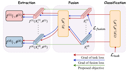
Figure 3: The gradient diagram extended from Figure 1, the notation system is consistent with Figure 1. The blue arrow represents the loss in the fusion stage ($\mathcal{L}_{fusion}$), and the red arrow represents the loss in the downstream task ($\mathcal{L}_{task}$). The green arrow is related to our redefined optimization objective, and the meaning is consistent with the green dashed arrow in Figure 1. Not all multimodal fusion methods have gradients with blue arrows and green arrows. These are not specific losses, nor are they necessarily individual losses.

The specific gradient backward diagram is shown in Figure 3. The gradient generated by the downstream task loss is propagated through the entire network to the input, and the gradient of the fusion stage loss (if any) is propagated from the fusion output feature to the downstream task. The parameter adjustment of the feature extractor is affected by the gradient backward of the loss in the fusion stage and the loss of the downstream task.

It is worth discussing that the gradient adjustments from downstream task classification loss and fusion-related loss may not necessarily align. Hence, there typically exists a set of hyperparameters to balance the impacts of different losses. For instance, in VAE [34], the KL divergence loss and the reconstruction loss serve distinct purposes. The KL divergence loss facilitates model generalization, a significant divergence between VAE and AE [35], while the reconstruction loss is task-specific, reconstructing a sample from the latent space. However, both the KL divergence loss and the reconstruction loss in VAE often cannot simultaneously be zero. The KL divergence loss encourages some randomness in the latent space features, whereas the reconstruction loss favors more consistency in the latent space features. This balancing act is commendable, yet weighting between the losses poses a significant challenge. Hence, when all losses in multi-stage learning bear significance and the gradient descent directions of feature extractors are incongruent, balancing a hyperparameter becomes necessary to harmonize diverse learning objectives.

However, not all losses bear significance. Take contrastive loss, for example. It is a downstream task loss in some NMT tasks [22], yet in most EMT tasks, contrastive loss typically operates in the fusion stage, complementing downstream task-relevant cross-entropy losses, to narrow the gap between positive samples in the latent space and push away negative samples. Some studies [1, 20] have demonstrated the existence of gaps between modalities, and smaller gaps are not necessarily better. There are also analyses of the behavior of contrastive loss [17], aiming to minimize mutual information for positive sample pairs and maximize mutual information for negative sample pairs [18].

In EMT tasks, if positive and negative sample pairs coexist, as in Audio-Visual Deepfake Detection [15], the contrastive loss in the fusion stage aims to extract consistent information from positive sample pairs (representing real samples) while ensuring inconsistency in negative sample pairs (representing fake samples). It must be emphasized that the significant advantage of EMT tasks lies in modality commonality. Some studies have proven the existence of commonality [36, 37], but this doesn’t alter the fact that auditory and visual modalities are fundamentally distinct (not only the semantic gap), with their enriched information not entirely consistent. In action recognition tasks, there is currently no work that effectively achieves this through audio; in speech recognition tasks [38], even with more complex, advanced feature extractors for extracting video features, or introducing priors to isolate video features solely for lip movements, the results are far inferior to audio single modality. While contrastive loss constrains the feature extractor to extract the most effective synchronous-related features, in the absence of a modality [15], it leads to a significant performance decline.

Moreover, not all tasks in EMT tasks involve positive and negative sample contrastive learning, so sometimes contrastive loss is equivalent to operating mutual information. For example, in some EMT methods’ decoupling works [8, 16], each modality enjoys a common encoder and a specific encoder, minimizing mutual information for different modalities’ common encoders to homogenize the extracted content and maximizing mutual information for the same modality’s common encoder and specific encoder to heterogenize them, adapting well to the environment of modality absence. However, this method fixes the dimensions of each feature part, and the introduced losses directly manipulate the behavior of the feature extractor, compelling it to extract a predetermined quantity of common and specific features. The design of hyperparameters (encoder dimensions) will alter the behavior of the feature extractor. Additionally, when expanding to more modalities, the training cost of this method is also worth discussing.

A.2 Combine With Residual

ResNet [29] solves the bottleneck of the number of network layers, and this epoch-making work allows the number of network layers to be stacked into thousands. A plausible explanation is that it reduces gradient disappearance or gradient explosion in deep networks. We try to explain this problem based on our information entropy related theory (Theory 3.1).

Figure 4: Structure of Residual in Networks.

The basic block structure of ResNet [29] and the gradient propagation are illustrated in Figure 4. We abstract it into a more general structure, where the downsampling block is considered as an arbitrary function $f(\cdot,\theta^{f})$, and the residual block is considered as another arbitrary function $g(\cdot,\theta^{g})$. Here, both of these arbitrary functions represent a type of network structure (in fact, this structure can be further generalized), with $\theta^{f}$ and $\theta^{g}$ representing the parameters of the functions $f$ and $g$, respectively. Same as Eq.(2), the objective of gradient optimization is to optimize these parameters to minimize the conditional entropy of Input $X,Y$ and Output $Y_{pred}$:

$$Y_{pred}=(g(f(X,\theta^{f})\ ,\theta^{g}),\quad\mathcal{L}=H[Y\ |\ g(f(X,\theta^{f})\ ,\theta^{g})]$$ (19)

The expression for gradient descent can be derived by computing the partial derivatives of the loss function with respect to the parameters $\theta^{f}$ and $\theta^{g}$. Denote the loss function as Eq.( 19), the gradient descent expressions are:

$$\frac{\partial\mathcal{L}}{\partial(\theta^{f},\theta^{g})}=\frac{\partial\mathcal{L}}{\partial\theta^{f}}+\frac{\partial\mathcal{L}}{\partial\theta^{g}},\quad\quad\frac{\partial\mathcal{L}}{\partial\theta^{f}}=\frac{\partial\mathcal{L}}{\partial g}\cdot\frac{\partial g}{\partial f}\cdot\frac{\partial f}{\partial\theta^{f}},\quad\quad\frac{\partial\mathcal{L}}{\partial\theta^{g}}=\frac{\partial\mathcal{L}}{\partial g}\cdot\frac{\partial g}{\partial\theta^{g}}$$ (20)

For functions $f$ positioned further back, their ultimate gradients are influenced by the partial derivatives of the loss function with respect to functions g positioned earlier. If network g is composed of $g_{1},g_{2},...,g_{n}$, then during backward, it will be multiplied by numerous coefficients, making it more prone to gradient vanishing or exploding. The introduction of residuals can alleviate this problem. It is expressed as:

$$Y_{pred}=(g(f(X,\theta^{f})\ ,\theta^{g})+f(X,\theta^{f})$$ (21)

These derivatives represent the directions of steepest descent with respect to the parameters $\theta^{f}$ and $\theta^{g}$, guiding the optimization process towards minimizing the loss function. Rethinking the associated gradient of $f$:

$$\frac{\partial\mathcal{L}}{\partial\theta^{f}}=\frac{\partial\mathcal{L}}{\partial g}\cdot\frac{\partial g}{\partial f}\cdot\frac{\partial f}{\partial\theta^{f}}+\frac{\partial\mathcal{L}}{\partial f}\cdot\frac{\partial f}{\partial\theta^{f}}$$ (22)

For the two elements of addition, compared to no residual, the first half of the gradient is numerically consistent, and the second half of the gradient is used as the residual. Obviously, this gradient is going to be direct.

Even in multimodal tasks, there exist challenges akin to residual issues yet to be resolved [39]. For instance, the association between feature extractors and downstream tasks may be compromised by the presence of feature fusion modules, manifested particularly in the introduction of intermediate gradients by deep fusion mechanisms, leading to gradient explosion or vanishing gradients. One approach to addressing this is through the incorporation of residuals. Indeed, some experimental endeavors have already undertaken this step, demonstrating its efficacy. These inferences may serve as a possible explanation, offering a generalized perspective.

However, residuals alone cannot entirely resolve the issue. Residuals, as a vector addition method, demand strict consistency in dimensions between inputs and outputs; moreover, excessive layer-by-layer transmission of residuals may result in the accumulation of low-level semantics onto high-level semantics, thereby blurring the representations learned by intermediate layers. While it may be feasible to employ residuals in a smaller phase within the fusion stage, utilizing residuals across the entire stage not only imposes stringent constraints on inputs and outputs but also risks semantic ambiguity.

Another method of applying residuals is akin to DenseNet [40], directly stacking channels. This still necessitates consistency in residual dimensions across different stages but circumvents the issue of semantic confusion. However, the final classifier remains a linear layer, requiring the flattening of multiple channels. Based on our theory, regardless of semantic sophistication, their initial origins remain consistent. As dimensions accumulate, elements describing the same set of features proliferate, inevitably leading to mutual information and subsequently reducing the conditional entropy relevant to downstream tasks.

In light of the foregoing analysis, residual connections at the skip-fusion stage can effectively alleviate the prevalent gradient issues in deep networks. However, this phased residual connection directly linking feature extractors to downstream tasks rigorously constrains the form of inputs and outputs, necessitating equilength features and overly blurred semantics, thus failing to achieve optimal effects. Furthermore, the nature of multimodal tasks diverges from simple downsampling-residual networks, as gradients stem not only from downstream tasks but also from multiple sources before the fusion stage. Our proposed method entails reducing the network layers in the fusion stage to align the fusion gradients with the descent direction of downstream task gradients. Alternatively, the scope of the fusion stage loss function gradient can be restricted.

Appendix B Proof of Theorem 3.4

We explain the derivation of the PNP equation to the proposed loss in detail. As before, let’s assume that the cell is one-dimensional, and only the direction $x$ exists.

Figure 5: Schematic diagram of the electrolytic cell, + (orange) and - (black) represent the charged species (ions and electrodes). There is a boundary $b$ (black line) in the electrolytic cell, assuming that the positive potential is $U_{0}$, the negative potential is $-U_{0}$, and the boundary $b$ is the zero potential.

For the basic Nernst-Planck equation, as shown in Figure 5, the ion $p\in\{+,-\}$ in the cell system conforms to:

$$\mathbf{J}_{p}=\underbrace{-D_{p}\nabla c_{p}(x,t)}_{\text{Diffusion}}+\underbrace{c_{p}(x,t)\mathbf{v}}_{\text{Advection}}+\underbrace{\frac{D_{p}z_{p}e}{k_{B}T}c_{p}(x,t)\mathbf{E}}_{\text{Electromigration}}$$ (23)

We abstract the feature vector into a one-dimensional electrolytic cell and need to correspond each term of the equation to it. Throughout the system, the fluid remains stationary; The electric field $\mathbf{E}$ that guides the movement of ions is generated by the electric potential $\phi$ and the magnetic field $\mathbf{A}$. We need to externally excite $\phi$ and do not additionally apply a magnetic field. The actual learning rate is usually not very large (< 100), and the charge of the ion is assumed to be very small. This gradient can be neglected as the magnetic field generated by the excitation.

$$\xLongrightarrow[\mathbf{v}\equiv\mathbf{0},\mathbf{A}\equiv\mathbf{0}]{\mathbf{E}=-\nabla\phi-\frac{\partial{\mathbf{A}}}{\partial{t}}}\underbrace{-D_{p}\nabla c_{p}(x,t)}_{\text{Diffusion}}+\underbrace{\frac{D_{p}z_{p}e}{k_{B}T}c_{p}(x,t)(-\nabla\phi)}_{\text{Electromigration}}$$ (24)

Our external excitation electric field is constant, so the potential expression can be expressed by the ion concentration.

$$\phi(x)=U_{0}+e\int_{0}^{x}(c_{+}(y,t)z_{+}+c_{-}(y,t)z_{-})dy$$ (25)

The final state of the system is that the flux is fixed with respect to time, that is, the partial differential is zero. From the ion point of view, diffusion and electromigration are in equilibrium.

$$\frac{\partial c_{p}(x,t)}{\partial t} =-\nabla\cdot\mathbf{J}_{p}\approx 0$$ (26)

$$\xLongrightarrow[]{}-\nabla\dot{\{}-D_{p}\nabla c_{p}(x,t)+\frac{D_{p}z_{p}e}{k_{B}T}c_{p}(x,t)[-\nabla\phi(x)]\}\approx 0$$ (27)

$$\xLongrightarrow[\text{using Poisson equation}]{\nabla^{2}\phi(x)=-\frac{\rho(x)}{\epsilon_{0}},\rho(x)=\sum_{j}z_{j}c_{j}(x,t)}$$ (28)

$$D_{p}(\frac{\partial^{2}c_{p}(x,t)}{\partial x^{2}}-\frac{z_{p}e}{k_{B}T\epsilon_{0}}c_{p}(x,t)\sum_{j}z_{j}c_{j}(x,t)+\frac{z_{p}e}{k_{B}T}\frac{\partial c_{p}(x,t)}{\partial x}\frac{d\phi(x)}{dx})\approx 0$$ (29)

Figure 6: Representation of ion distribution. The ordinate represents the ion concentration and the abscissa represents the electrolytic cell position. 0 is the position of the positive electrode, $l$ is the position of the negative electrode, and $b$ is the potential equilibrium boundary. The green line represents a uniform distribution of initial state ions to conform to macroscopic electrical neutrality, the yellow line represents the ideal electrolysis target, that is, the foreign ions are completely divided at the equilibrium boundary, and the red line represents the practically possible situation.

In the initial condition, ions undergo spontaneous and uniform distribution through diffusion driven by Brownian motion (the green line in Figure 6). This dynamic process leads to the establishment of a heterogeneous distribution of ions within the system. However, as the system approaches the potential equilibrium boundary $b$, the electrostatic forces acting on ions become increasingly influential. At this boundary, denoted as the end condition [41], the principles of electroneutrality come into play. Here, positive and negative ions are balanced such that their net charge is neutral, resulting in an electrically neutral region around the potential equilibrium boundary:

$$\sum_{j}z_{j}c_{j}(x,t)\approx 0,\quad\frac{\partial^{2}c_{p}(x,t)}{\partial x^{2}}+\frac{z_{p}e}{k_{B}T}\frac{\partial c_{p}(x,t)}{\partial x}\frac{d\phi(x)}{dx}\approx 0$$ (30)

$$\phi(x)=\phi(0)-\int_{0}^{x}E(y)dy=\phi(0)+\int_{0}^{x}\int_{0}^{y}\frac{\rho(z)}{\varepsilon_{0}}dzdy$$ (31)

$$\phi(0)-\phi(b)\approx\frac{k_{B}T}{z_{+}e}\ln\left(\frac{c_{+}^{0}}{c_{+}(b)}\right)$$ (32)

The positive and negative properties of diffusion and electromigration are always opposite. If the ion species used as the external electrode is the same as that of the original solution, then we can approximately assume that the ion on either side of the zero potential boundary $b$, combined with the ion equivalent to the external electrode, can reduce the initial solute.

Assuming features from another modality are perfectly ordered, they can serve as a constant stimulus guiding the ionization of the awaiting electrolytic modality. However, unlike in deep learning, where the loss function can be equivalent to an external potential, both serve as stimuli capable of guiding the respective fundamental ion directional motion.

Beginning with two modalities, initially disordered features prompt GMF to attempt cyclic connections, as depicted in the diagram. The imposition of external guidance induces the movement of feature particles of different polarities in distinct directions, ultimately coalescing at one end. According to the law of conservation of mass, these aggregated features can be fully reconstructed into the original modality representation of the guided modality particles at the opposite end.

Expanding to multiple modalities, electrochemical cells allow for parallel multi-level connectivity, where applying a set of stimuli can simultaneously guide the movement of ions across multiple cell groups. These potentials, as per the principles of basic circuitry, are distributed across each cell, as shown in Figure 7.

Figure 7: Example diagram of loop guidance. The modes are excited by each other.

The PNP equation provides a theoretical basis for GMF, and then we can propose to model material conservation with a reconstruction loss. The reconstruction loss can well simulate the motion of particles, and its reduction condition does not lead to ambiguity due to the existence of modality-specific, as expressed in Eq.( 32).

Appendix C Proof of Theorem 3.2

Theorem 3.2: The dimension of the feature that is best suited to the downstream task varies, and there is always an optimal value for this feature. The dimension multiple relationship between each layer of the feature extractor is fixed, and the initial dimension is adjusted. Too low dimension of the final output will lead to inefficient representation, and too high dimension will introduce noise. The existence of an integer $l_{\text{best}}$ such that for any integer $l$ distinct from $l_{\text{best}}$, the conditional entropy of the model’s predictions $f_{l}(X,\theta_{l})$ is greater than that of the model’s predictions $f_{l_{\text{best}}}(X,\theta_{l_{\text{best}}})$.

$$\exists l_{\text{best}}\in\mathbb{N},\forall l\in\mathbb{N},l\neq l_{\text{best}},H(Y|f_{l}(X,\theta_{l}))>H(Y|f_{l_{\text{best}}}(X,\theta_{l_{\text{best}}}))$$ (33)

C.1 Experiment

There was some previous work [42] that demonstrated that this optimal dimension exists. However, existing methods do not account particularly well for the conditions under which poor fitting occurs, so we conduct experiments to demonstrate the existence of this phenomenon. At the end we present a possible conjecture. The existence of this optimal dimension is universal and at the same time inconsistent. Specifically, each type of feature extractor, each type of dataset, and each corresponding downstream task have different optimal dimensions.

Our set of experiments is shown in Fig LABEL:fig:level. In addition to the intuitive visualization of the validation accuracy, we also show the ratio of the validation accuracy to the training accuracy, aiming to measure the validation accuracy and reflect the fitting effect of the model. The closer the ratio is to 1, the stronger the generalization ability is, and the better the fit is.

In Figure LABEL:fig:level (a) and (b), the evaluation results of ResNet [29] on CIFAR-10 [43] are presented. As the dimensionality increases, the testing performance of the model improves, and the performance range stabilizes. However, with a twofold increase in dimensionality, the variation in testing performance diminishes, approaching zero. In other words, doubling the parameter count does not yield any improvement. Additionally, for larger networks like ResNet110, performance begins to decline. Furthermore, while absolute performance is increasing, the ratio is declining, indicating a weakening in generalization capability.

Figure LABEL:fig:level (c) and (d) depict the evaluation results of MobileNetV3 [44] on CIFAR-10 [43], showing conclusions similar to those of ResNet. For larger networks like MobileNetV3-Large, at lower dimensionalities, its generalization capability is significantly lower compared to simpler networks.

Figure LABEL:fig:level (e) and (f) illustrate the evaluation results of ViT [45] on CIFAR-10 [43]. As ViT is based on transformers [27] and possesses a global receptive field, its base dimensionality is significantly larger than that of convolutional neural networks. Both in terms of absolute performance and ratio, its optimal representation dimensionality approaches 256, distinct from other networks.

However, it is worth noting that the presence of optimal features is not only closely related to network type and structure, but also to the dataset and downstream tasks. We chose CIFAR-100 [43] for this set of comparative experiments. This is because its data volume is consistent with CIFAR-10, but with more categories and greater difficulty. The experimental results of ResNet [29] evaluated on CIFAR-100 are shown in Figure LABEL:fig:cf100. Compared to the results shown in Figure LABEL:fig:level(a) and (b), firstly, the impact of different dimensions on accuracy is more significant (for example, the maximum difference in test performance of ResNet-20 on CIFAR-10 is about 25%, exceeding 40% here); for ResNet-110, excessive dimensions no longer lead to performance stabilization, but rather a visible performance decline.

The experimental results demonstrate the existence of an optimal dimensionality. This dimensionality may vary based on the different structures of networks. Hence, the concept of optimal dimensionality should be discussed in consideration of multiple external conditions.

Appendix D Proof of Theorem 3.3

Theorem 3.3: The feature extractor is fixed, and its original output feature dimension $l$ is mapped to $nl$, and finally back to $l$. The mapping result is used as the basis for the downstream task. The performance of downstream tasks is infinitely close to the original performance as $n$ increases, but never greater than the original performance. For magnification $n>1,n\in\mathbb{Z}$, mapping matrix $\textbf{U}_{1}\in\mathbb{R}^{l\times nl}$ and $\textbf{U}_{2}\in\mathbb{R}^{nl\times l}$, For the output features $f(X,\theta)\in\mathbb{R}^{l}$ and $Y$:

$$H(Y|f(X,\theta))<H(Y|\textbf{U}_{1}\cdot(\textbf{U}_{2}\cdot f(X,\theta)))$$ (34)

$$lim_{n\to\infty}H(Y|\textbf{U}_{1}\cdot(\textbf{U}_{2}\cdot f(X,\theta))))=H(Y|f(X,\theta)$$ (35)

D.1 Theoretically

Denote $V=f(X,\theta)$, the rank of each stage:

$$V=\begin{bmatrix}v_{1}\\ v_{2}\\ \vdots\\ v_{l}\end{bmatrix},\quad r(V)\leq l,\quad r(\textbf{U}_{2})\leq l,\quad r(\textbf{U}_{2}\cdot V)\leq\min(r(V),r(\textbf{U}_{2}))\leq l,$$ (36)

$$r(\textbf{U}_{1})\leq l\quad r(\textbf{U}_{1}\cdot(\textbf{U}_{2}\cdot f(X,\theta))\leq l$$ (37)

The mapped rank is always less than or equal to the original rank. That is, downstream task-relevant features may be compressed while not generating features out of thin air. Eq. (34) gets the certificate. For Eq.(35), we discuss the problem from pruning, linear algebra and probability theory. Neural networks are often overparameterized, requiring more network parameters than needed to get a good fit. In theory [23], however, only a subset of these parameters are useful in practice. Hence, some knowledge distillation methods such as teacher-student networks and pruning [46]. These tested models maintain good performance while removing most of the parameters, which proves that overparameterization is a common phenomenon. We interpret it as a probabilistic problem, that is, the effective parameters are generated with a certain probability. Overparameterization significantly improves the effective parameter generation, and knowledge distillation removes these redundant and invalid parameters.

Let $\mathbf{A}\in\mathbb{R}^{nd\times d}$ be a learnable matrix ($n>>1$). Act on $\mathbf{v}\in\mathbb{R}^{d}$ to complete the mapping from lower dimension to higher dimension:

$$\mathbf{A}=[\mathbf{a_{1}},\mathbf{a_{2}},\dots,\mathbf{a_{nd}}],\quad\hat{\mathbf{v}}=\mathbf{Av}=[\hat{\mathbf{v}}_{1},\hat{\mathbf{v}}_{2},\dots,\hat{\mathbf{v}}_{nd}]^{\text{T}}$$ (38)

Denote $\hat{\mathbf{v}}\in\mathbb{R}^{nd}$ as the mapping result. $\hat{\mathbf{v}}_{k}$ represents the $k$-th row element. For any two of these row vectors $\mathbf{a_{i}}$ and $\mathbf{a_{j}}$ ($i\neq j$). They have a ratio c for their first elements.A necessary and sufficient condition for linearity between two vectors can be extended to the following: for any element in the same row of these two vectors, the ratio should be $c$.

$$\mathbf{a_{i}}=[a_{i1},a_{i2},\dots,a_{id}],\quad\mathbf{a_{j}}=[a_{j1},a_{j2},\dots,a_{jd}],\quad c=\frac{a_{i1}}{a_{j1}}$$ (39)

$$\sum_{t=1}^{d}\frac{a_{jt}}{a_{it}}=c$$ (40)

If $\mathbf{A}$ is learnable, each element will have a different weight for each parameter adjustment. denote $\text{P}(\frac{a_{jt}}{a_{it}}=c)$ as the probability that the proportion of the $t$-th element of $\mathbf{a_{i}}$ and $\mathbf{a_{j}}$ is equal to $c$, which cannot be determined directly because the input sample is uncertain. In the context of neural networks, the adjustment of gradients can be regarded as following a continuous probability distribution. Consequently, the probability of the adjustment taking on a specific constant value is zero (does not imply impossibility). By cumulatively multiplying this probability, we get the probability that the two column vectors are linearly related in gradient descent.

$$\prod_{t=1}^{d}\text{P}(\frac{a_{jt}}{a_{it}}=c)\approx 0$$ (41)

However, for a $d$-dimensional vector, there cannot be more than $d$ linearly independent features. To simplify the expression, we assume that Eq.(41) is a fixed value on the interval (0,1). The probability that exactly d-dimensional features are linearly dependent is given by:

$$\frac{(nd)!}{d!(nd-d)!}(\prod_{t=1}^{d}\text{P}(\frac{a_{jt}}{a_{it}}=c))^{d}(1-\prod_{t=1}^{d}\text{P}(\frac{a_{jt}}{a_{it}}=c))^{nd-d}$$ (42)

$$\frac{(nd+1)!}{d!(nd+1-d)!}(\prod_{t=1}^{d}\text{P}(\frac{a_{jt}}{a_{it}}=c))^{d}(1-\prod_{t=1}^{d}\text{P}(\frac{a_{jt}}{a_{it}}=c))^{nd+1-d}$$ (43)

In deep learning methods, the feature dimension is usually not set too small, $d$ is sufficiently large. Combined with gradient descent, the parameter adjustment is random, the linear correlation probability of two random features is close to 0.

$$\prod_{t=1}^{d}\text{P}(\frac{a_{jt}}{a_{it}}=c)\approx 0,\quad\frac{Eq.(\ref{equ:pn+m})}{Eq.(\ref{equ:pn})}=\frac{nd+1}{nd+1-d}\prod_{t=1}^{d}\text{P}(\frac{a_{jt}}{a_{it}}=c)\approx 1+\frac{d}{nd+1-d}\geq 1$$ (44)

Consider mapping matrix $\textbf{U}_{2}\in\mathbb{R}^{nl\times l}$. As n increases, the probability of rank $l$ increases. The same is true for the matrix $\textbf{U}_{1}\in\mathbb{R}^{l\times nl}$. Therefore, as the probability of two correlation matrices being full rank becomes larger, a larger $n$ helps to restore the original representation under the premise that the network does not involve unexpected situations such as gradient explosion and vanishing gradients. However, it can be determined that when n is less than 1 (n > 0), there must be information loss. This is because the upper limit of the rank of a matrix depends on the smaller value of the number of rows, columns. Furthermore, it is not appropriate to increase the number of parameters blindly, which will lead to an exponential number of parameters.

D.2 Experiment

Figure 13: Theoretical validation on ImageNet on the performance impact of raising and then reducing the original features. The horizontal coordinate represents the mapped feature dimension, the upper bound is the best performance, the lower bound is the worst performance, and the ordinate represents the validation set accuracy. The dashed line represents the results reported for directly validating the performance of the pretrained model.

We employed pre-trained ResNet-18, ResNet-34, ResNet-50, and ResNet-101 [29] models provided by PyTorch [47], removing their classifiers to obtain raw features with dimensions of 512, 512, 2048, and 2048 respectively. After freezing the other layers, we mapped these original features to another dimension and subsequently retrained the classifiers based on these new features. As depicted in Figure 13, where the abscissa represents the dimensions of the mapped features and the ordinate represents the classification accuracy of the new classifier on the ImageNet [48] validation set. Our experimental hyperparameter design and optimizer were identical to those reported in the original paper. We recorded the validation accuracy every 400 iterations, and if the accuracy did not improve for 10 consecutive validations, training was terminated prematurely. The final results are depicted in a bar chart, where the upper and lower bounds represent the maximum and minimum values of the validation accuracy.

It can be observed that larger mapping dimensions lead to faster convergence and yield better results. Smaller mapping dimensions, especially when they are smaller than the original dimensions, not only exhibit significant differences in upper and lower bounds of validation accuracy but also witness a substantial decrease in the upper limit. This observation aligns with our theoretical expectations. When the scaling factor $n$ is close to 4, the performance loss has entered the acceptable range.

Appendix E Different Between Theorem 3.2 and Theorem 3.3

Both Theorem 3.2 and Theorem 3.3 focus on the dimension of presentation. The most significant difference between the two theories is what the original input was.

Theorem 3.2 is for the case where the sample is known and the representation is unknown, and this representation contains relevant information and irrelevant information. Therefore, this theory is more about the number of parameters needed to characterize, the minimum dimension needed to get the best performance, or the best performance in the minimum dimension. In this paper, this theory emphasizes the necessity of unequal-length fusion, and points out and proves through experiments that equal-length fusion may bring the problem of feature redundancy or feature missing, which not only increases the unnecessary amount of computation, but also affects the performance to some extent.

Theorem 3.3 is to analyze the influence of linear mapping on the representation in the case of known representation and unknown samples. Our proposed GMF method is very simple and contains only a number of linear layers, achieving the performance of larger parameter fusion methods of previous works. However, our original intention is not to be guided by experimental results, but to theoretically analyze whether the possible information loss is acceptable. We expect our work to be interpretable and applicable.

Appendix F Derivation of Conjecture 3.1

Conjecture 3.1: Rely on Theorem 3.1, 3.2, 3.3, we propose an conjecture that a boundary of performance limitation exists, determined by downstream-related entropy. Theoretically, by establishing a direct correspondence between the extractor and classifier, fusion method can enhance the limitation boundary, further improve performance.

Based on the proof of Theorem 3.2, one of the foundations of learning in neural networks is gradient descent, which presuppositions that gradients can be backpropagated. Every tuning of the learnable parameters will eventually be implemented on the original input. Assuming that the feature extractor is fixed, the original input at this time is the feature output by the feature extractor. For any learnable parameter, the value of a certain sample can be expressed by an exact formula. For a completely consistent input, it is assumed that its downstream task-related information entropy can be efficiently calculated, and its information entropy minimum is certain. Therefore, there is a performance upper bound, depending on how the existing features are utilized.

In practical deep learning tasks, the input features are often not fixed, and gradients need to propagate to be able to fully determine the original samples—which must also be fully determined. We continue to analyze the feature layers outputted by the feature extractor, assuming that the relevant information entropy of downstream tasks can be manually calculated. Thus, for the output features at a certain moment, the lower bound of the conditional entropy of downstream tasks can still be computed, which represents the performance upper bound.

Therefore, the entire multimodal learning network is divided into two parts: one is the lower bound of the conditional entropy of the feature extractor output relative to the original samples, and the other is the lower bound of the conditional entropy of downstream tasks relative to the feature extractor output. The former is a prerequisite for the latter sequentially. However, as stated in the formulas, assuming the existence of fusion loss and downstream task loss, and the gradient descent directions are not completely consistent, let the weight of the fusion loss $\mathcal{L}_{fusion}$ be $\lambda_{1}$, and the loss of the downstream task $\mathcal{L}_{task}$ be $\lambda_{2}$, the total loss can be expressed as:

$$\mathcal{L}=\lambda_{1}\mathcal{L}_{fusion}+\lambda_{2}\mathcal{L}_{task}$$ (45)

The learning task is to minimize the training loss. Assuming that $\lambda_{1}\mathcal{L}_{fusion}>\lambda_{2}\mathcal{L}_{task}$, then the gradient of the feature extractor will tend more toward the fusion loss. In severe cases (such as opposite gradient descent directions), the downstream task-related loss will be completely overshadowed. This also leads to an increase in the lower bound of the conditional entropy of downstream tasks and a decrease in the theoretical performance upper limit. Therefore, we assume that there exists a boundary, which is determined by the theoretical performance upper bound based on a fixed feature and the conditional entropy of downstream tasks. Regardless of how outstanding the fusion method design is, just like the principle of energy conservation law for features, the final task performance of this method cannot exceed this upper bound.

Figure 14: Visualizing performance improvements based on conjectures.

The reason why our proposed GMF achieves performance improvement is not due to the performance enhancement brought by the complex fusion network, but rather from a higher upper bound. However, in reality, we are still far from this upper bound, and demonstrating our method as a precursor to other methods can prove this point well. As shown in the Figure 14, we have drawn a hypothetical graph based on the data reported in the paper. Assuming GMF as the precondition method for the Perceiver [4], the result that GMF can be on par with complex networks with almost no resource consumption is interpretable.

Appendix G Experiment Supplement

G.1 Implement Details

For all experiments, we use apex to optimize the v-memory and the parameter is set to ’O1’. The random seed fixed ’1’ for all GMF related implementation. However, for some dropout design methods, the reported experimental results may not be fully reproducible. More details are listed in Table  5

1. torch.manual_seed(seed)

2. torch.cuda.manual_seed_all(seed)

3. np.random.seed(seed)

4. random.seed(seed)

Table 5: Details of GMF. Momentun of SGD = 0.9, weight delay=1e-4. Lr_scheduler = ReduceLROnPlateau, factor=0.1, patience=1000.

Dataset	Lr	Optimizer	Batchsize	Epoch	Input Shape
VGGSound	0.01	SGD	64	20	[512,512]
ActivityNet	0.01	SGD	64	20	[4096,128], [4096,4096], [128,128]
FakeAVCeleb	0.01	SGD	64	20	[512,512], [128,512]

G.2 Information About Preprocess and Baseline

For the VGGSound dataset, we downsample all currently available samples to 5fps, with videos of size 192*256 and audio sampled at 16000 Hz, while retaining only the first 9 seconds to accommodate most samples that are not exactly 10 seconds in duration. Samples without audio or video are removed. As for FakeAVCeleb, since the fabricated samples exhibit a global range of fabrication, with lengths distributed from 0.8 seconds and above, and a frame rate between 15 to 30 fps, we only select the first 8 frames along with their corresponding audio to ensure adaptability to the dataset.

We employ the default testing-training split provided by VGGSound. For FakeAVCeleb, consistent with much of the prior work focused on audio-visual deepfake detection, we first sort each class (real audio-real video, real audio-fake video, fake audio-real video, fake audio-fake video), and then allocate the first 70% of each class to the training set and the remaining 30% to the testing set.

The baseline of VGGSound pretrained on KINETICS400V1. Momentun of SGD = 0.9, weight delay=1e-4. Adam betas=(0.5, 0.9). lr_scheduler = ReduceLROnPlateau, factor=0.1, patience=1000 on VGGSound, factor=0.5, patience=50, verbose=True, min_lr=1e-8 on FakeAVCeleb. The generated audio sequence is quite long, and the receptive field of the convolutional network is not global. To address this potential issue, we stack the audio into a timing sequence (144000 to 9 $\times$ 16000).

Audio wave transform to input tensor by MelSpectrogram(sample_rate=16000, n_fft=400, win_length=400, hop_length=160, n_mels=192) for VGGSound and log (abs (STFT(n_fft=1024, hop_length=256, win_length=1024,window=blackman_window(1024))) + 1e-8) for FakeAVCeleb. Video frame directly as the input of network without any preprocess.

The hyperparameter as shown in Table 6

Table 6: Model Details of Baseline.

Model	Modality	Dataset	Role	Lr	Optimizer	Batchsize	Epoch	Input Shape
R2+1D-18	A	VGGSound	Baseline	0.01	SGD	64	20	[9,192,100,1]
R2+1D-18	V	VGGSound	Baseline	0.01	SGD	64	20	[15,128,96,3]
R2+1D-18	A	FakeAVCeleb	Baseline	0.005	Adam	16	5	[1,1,513,60]
R2+1D-18	V	FakeAVCeleb	Baseline	0.005	Adam	16	5	[8,224,224,3]

G.3 Compared Method Structure

The integration of our method with others is depicted in Figure 1. By bypassing modality-invariant features and focusing solely on modality-specific features for fusion, the input represents a representation with reduced mutual information. This leads to a reduction in the conditional entropy magnitude during the initial stages. The backend component may consist of a simple concatenation or modules proposed by other methods. Consequently, the inherent characteristics of GMF are constrained by the limitations of the backend module. Comparatively, the limitations are minimal with a simple concatenation approach.

Figure 15: G-structure schematic diagram. Yellow feature vectors represent modality-invariant features, while other colors represent modality-specific features for each modality. Modality-invariant features are directly connected to downstream task classifiers, while modality-specific features serve as new inputs to the fusion module.

Appendix H More Comparison on the FakeAVCeleb Dataset

Table 7: Performance on the FakeAVCeleb dataset. ’A’, ’V’ represents the separate audio and video modality, and the input of the other modality is 0. ’AV’ stands for the full sample.

Method	Extractor	ACC(%)			AUC(%)
		A	V	AV	A	V	AV
Baseline	R(2+1)D-18 [28]	98.76	95.36	97.68	99.73	54.38	69.33
MISA [16]	sLSTM [30]	61.75	71.66	97.68	58.98	64.76	79.22
UAVM [6]	ConvNeXT-B [31]	86.59	73.05	78.64	83.98	69.38	43.92
DrFuse [8]	R(2+1)D-18 [28]	66.83	75.35	97.68	62.86	69.33	78.56
Perceiver [4]	R(2+1)D-18 [28]	56.81	78.84	97.68	51.36	58.20	93.45
Joint-AV [49]	R(2+1)D-18 [28] and 1D CNN	81,77	65.73	71.81	79.25	69.61	75.81
AVoiD-DF [15]	ViT [45]	70.31	55.81	83.71	72.41	57.21	89.21
VFD [50]	Transformer [27]	-	-	81.52	-	-	86.11
Emo-Foren [51]	2D CNN and MFN [52]	-	-	78.11	-	-	79.81
MDS [53]	3D-ResNet [54] Like	-	-	83.86	-	-	86.71
GMF	R(2+1)D-18 [28]	71.25	85.33	97.68	67.32	64.91	91.88
GMF-Perceiver	R(2+1)D-18 [28]	64.01	82.15	98.21	66.53	62.42	96.71
GMF-MAE	MAE [32] and Audio-MAE [33]	99.79	97.74	99.99	99.73	89.82	99.97

We expanded the experimental table of FakeAVCeleb (Tab. 4) in the main text, incorporating additional comparisons focused on deepfake detection methods. Apart from the experiments reported in the original text, the remaining data were sourced from the original paper proposing the method. Here, VFD [50], Emo-Foren [51], and MDS [53] are grouped together because these methods transform EMT into NMT. Specifically, these methods emphasize certain aspects of multimodal performance: VFD emphasizes identity, Emo-Foren emphasizes emotion, and MDS, while not emphasizing a specific mode, relies on computing confidence in matching a certain segment. Therefore, the modal absence evaluation for these methods is marked as ’-’, indicating absence. Importantly, our method effectively connects representations of different modalities without additional overhead for AE-based feature extractors, resulting in a highly competitive outcome.

H.1 The reason of choose FakeAVCeleb

The FakeAVCeleb dataset is atypical, characterized by severe class imbalance posing significant challenges to methods. Specifically, the ratio of positive to negative samples is 1:1 for audio and 1:19 for video, resulting in an overall ratio of 1:39. While audio often possesses discriminative capabilities less susceptible to the impact of sample proportions, most methods evaluated in our tests struggle to effectively address this bias.

Addressing this imbalance necessitates multimodal methods to learn weight disparities across modalities to mitigate the effects of sample bias. This manifests in high accuracy (ACC) juxtaposed with mismatched area under the curve (AUC). Methods capable of mitigating this bias often underutilize it, resulting in suboptimal ACC. However, in real-world scenarios, the distribution of genuine and fake samples may not be balanced, and a single segment may not adequately represent an event. Hence, the adaptability of methods to publicly available datasets warrants thorough investigation.

Appendix I GMF with AutoEncoder (GMF-AE/MAE)

AutoEncoder [35] (AE) was initially proposed as a feature dimensionality reduction method, compressing samples into a latent space and then reconstructing them to retain the details of the entire sample in the latent space features. Masked AutoEncoder [32] (MAE) is a more powerful feature extraction variant of AE, masking most of the original samples and reconstructing them, allowing the model to learn more sample features. An intriguing point is that this concept can be seamlessly integrated with GMF (proposed Generalized Multimodal Fusion).

Figure 16: Simplified GMF frame diagram with MAE as feature extractor.

GMF applies reconstruction loss as an incentive, directing the movement of different types of features towards a relatively ordered representation. Combining with PNP equations and our theoretical framework, this requires two additional linear layers for feature dimensionality reduction, expansion, and a linear layer for reconstruction. Thus, the additional overhead includes a reconstruction loss and the mentioned linear layers. However, due to the nature of AE, this feature-directional movement process can be accomplished during AE’s self-supervised learning. Specifically, instead of feeding complete latent space features into the Decoder, a combination of features from the corresponding Encoder and another modality Encoder is used. This allows us to achieve our goal without any additional overhead. However, if done so, explicit boundary delineation is necessary, which may affect model performance; moreover, this learning process must be conducted in a multi-modal task, and features must be intact during the learning process.

The specific structural diagram is shown in Figure 16. Here, we also consider the transformer [27] initially used for text as a variant of MAE, video encoder is MAE [32] and the Audio encoder is Audio-MAE [33].

Appendix J GMF Architecture

Algorithm 1 GMF (Generalized Multimodal Fusion)

1:Input: Dimensions $dims$, multiple $m$, boundary $b$

2:Output: $x1$, $x2$, $x1_{\text{recon}}$, $x2_{\text{recon}}$

3:procedure GMF($x1$, $x2$)

4:     $x1_{\text{inv}},x1_{\text{spec}}\leftarrow$ ElementSplit($x1$, $dims[0]$, $\text{min}(dims)$, $m$, $b$)

5:     $x2_{\text{inv}},x2_{\text{spec}}\leftarrow$ ElementSplit($x2$, $dims[1]$, $\text{min}(dims)$, $m$, $b$)

6:     $x1\leftarrow\text{concat}([x2_{\text{inv}},x1_{\text{spec}}])$

7:     $x2\leftarrow\text{concat}([x1_{\text{inv}},x2_{\text{spec}}])$

8:     $x1_{\text{re}}\leftarrow\text{Linear}(x1,dims[0]+\text{min}(dims),dims[0])$

9:     $x2_{\text{re}}\leftarrow\text{Linear}(x2,dims[1]+\text{min}(dims),dims[1])$

10:     return $x1$, $x2$, $x1_{\text{re}}$, $x2_{\text{re}}$

11:end procedure

Algorithm 2 ElementSplit

1:Input: Dimension $dim$, min_len, multiple $m$, boundary $b$

2:Output: $x_{\text{inv}}$, $x_{\text{spec}}$

3:procedure ElementSplit($x$)

4:     $b\leftarrow\lfloor b\times m\times dim\rfloor$

5:     $d\leftarrow m\times dim$

6:     $x\leftarrow\text{Linear}(x,dim,m\times dim)$

7:     $x_{\text{inv}}\leftarrow\text{Linear}(x[:,:b],b,\text{min\_len})$

8:     $x_{\text{spec}}\leftarrow\text{Linear}(x[:,b:d],d-b,dim)$

9:     return $x_{\text{inv}}$, $x_{\text{spec}}$

10:end procedure

Algorithm 3 Reconstruction Loss

1:Input: $x_{\text{recon}}$, $x_{\text{original}}$

2:Output: Reconstruction loss

3:procedure ReconstructionLoss($x_{\text{recon}}$, $x_{\text{original}}$)

4:     return $\text{MSE}(x_{\text{recon}},x_{\text{original}})$

5:end procedure

References

- [1] Liang, V. W., Y. Zhang, Y. Kwon, et al. Mind the gap: Understanding the modality gap in multi-modal contrastive representation learning. In Advances in Neural Information Processing Systems, pages 17612–17625. 2022.
- [2] Xia, Y., H. Huang, J. Zhu, et al. Achieving cross modal generalization with multimodal unified representation. In Conference and Workshop on Neural Information Processing Systems, pages 63529–63541. 2023.
- [3] Nagrani, A., S. Yang, A. Arnab, et al. Attention bottlenecks for multimodal fusion. In Conference and Workshop on Neural Information Processing Systems, pages 14200–14213. 2021.
- [4] Jaegle, A., F. Gimeno, A. Brock, et al. Perceiver: General perception with iterative attention. In International Conference on Machine Learning. 2021.
- [5] Liu, L., J. Li, L. Niu, et al. Activity image-to-video retrieval by disentangling appearance and motion. In Association for the Advancement of Artificial Intelligence. 2021.
- [6] Gong, Y., A. H. Liu, A. Rouditchenko, et al. Uavm: Towards unifying audio and visual models. IEEE Signal Processing Letters, pages 2437–2441, 2022.
- [7] Ying, X. An overview of overfitting and its solutions. Journal of Physics: Conference Series, page 022022, 2019.
- [8] Yao, W., K. Yin, W. K. Cheung, et al. Drfuse: Learning disentangled representation for clinical multi-modal fusion with missing modality and modal inconsistency. In Association for the Advancement of Artificial Intelligence, pages 16416–16424. 2024.
- [9] Ma, M., J. Ren, L. Zhao, et al. Are multimodal transformers robust to missing modality? In IEEE/CVF Conference on Computer Vision and Pattern Recognition. 2022.
- [10] Wang, H., Y. Chen, C. Ma, et al. Multi-modal learning with missing modality via shared-specific feature modelling. In 2023 IEEE/CVF Conference on Computer Vision and Pattern Recognition, pages 15878–15887. 2023.
- [11] Kim, W., B. Son, I. Kim. Vilt: Vision-and-language transformer without convolution or region supervision. In International Conference on Machine Learning. 2021.
- [12] Li, J., R. R. Selvaraju, A. D. Gotmare, et al. Align before fuse: Vision and language representation learning with momentum distillation. In NeurIPS, pages 9694–9705. 2021.
- [13] Dou, Z.-Y., Y. Xu, Z. Gan, et al. An empirical study of training end-to-end vision-and-language transformers. In IEEE/CVF Conference on Computer Vision and Pattern Recognition, pages 18145–18155. 2021.
- [14] Xu, R., L. Niu, J. Zhang, et al. A proposal-based approach for activity image-to-video retrieval. In Association for the Advancement of Artificial Intelligence, pages 12524–12531. 2020.
- [15] Yang, W., X. Zhou, Z. Chen, et al. Avoid-df: Audio-visual joint learning for detecting deepfake. IEEE Transactions on Information Forensics and Security, pages 2015–2029, 2023.
- [16] Hazarika, D., R. Zimmermann, S. Poria. Misa: Modality-invariant and -specific representations for multimodal sentiment analysis. In ACM International Conference on Multimedia, pages 1122–1131. 2020.
- [17] Wang, F., H. Liu. Understanding the behaviour of contrastive loss. pages 2495–2504. 2020.
- [18] Boudiaf, M., J. Rony, I. M. Ziko, et al. A unifying mutual information view of metric learning: Cross-entropy vs. pairwise losses. In European Conference on Computer Vision, page 548–564. 2020.
- [19] Shang, Z. W., W. Li, M. Gao, et al. An intelligent fault diagnosis method of multi-scale deep feature fusion based on information entropy. Chinese Journal of Mechanical Engineering, 2021.
- [20] Jiang, Q., C. Chen, H. Zhao, et al. Understanding and constructing latent modality structures in multi-modal representation learning. In IEEE/CVF Conference on Computer Vision and Pattern Recognition, pages 7661–7671. 2023.
- [21] Granada, J. R. G., V. A. Kovtunenko. Entropy method for generalized poisson–nernst–planck equations. Analysis and Mathematical Physics, pages 603–619, 2018.
- [22] Radford, A., J. W. Kim, C. Hallacy, et al. Learning transferable visual models from natural language supervision. In International Conference on Machine Learning, pages 8748–8763. 2021.
- [23] Frankle, J., M. Carbin. The lottery ticket hypothesis: Finding sparse, trainable neural networks. In International Conference on Learning Representations. 2019.
- [24] Heilbron, F. C., V. Escorcia, B. Ghanem, et al. Activitynet: A large-scale video benchmark for human activity understanding. In 2015 IEEE Conference on Computer Vision and Pattern Recognition, pages 961–970. 2015.
- [25] Chen, H., W. Xie, A. Vedaldi, et al. Vggsound: A large-scale audio-visual dataset. In 2020 IEEE International Conference on Acoustics, Speech and Signal Processing, pages 721–725. 2020.
- [26] Khalid, H., S. Tariq, M. Kim, et al. Fakeavceleb: A novel audio-video multimodal deepfake dataset. In Proceedings of the Neural Information Processing Systems Track on Datasets and Benchmarks. 2021.
- [27] Vaswani, A., N. M. Shazeer, N. Parmar, et al. Attention is all you need. In Neural Information Processing Systems. 2017.
- [28] Tran, D., H. Wang, L. Torresani, et al. A closer look at spatiotemporal convolutions for action recognition. In Proceedings of the IEEE Conference on Computer Vision and Pattern Recognition, pages 6450–6459. 2018.
- [29] He, K., X. Zhang, S. Ren, et al. Deep residual learning for image recognition. In 2016 IEEE Conference on Computer Vision and Pattern Recognition, pages 770–778. 2016.
- [30] Hochreiter, S., J. Schmidhuber. Long short-term memory. Neural Computation, pages 1735–1780, 1997.
- [31] Todi, A., N. Narula, M. Sharma, et al. Convnext: A contemporary architecture for convolutional neural networks for image classification. In 2023 3rd International Conference on Innovative Sustainable Computational Technologies (CISCT), pages 1–6. 2023.
- [32] He, K., X. Chen, S. Xie, et al. Masked autoencoders are scalable vision learners. In Proceedings of the IEEE/CVF Conference on Computer Vision and Pattern Recognition, pages 16000–16009. 2022.
- [33] Huang, P.-Y., H. Xu, J. B. Li, et al. Masked autoencoders that listen. In Advances in Neural Information Processing Systems. 2022.
- [34] Kingma, D. P., M. Welling. Auto-encoding variational bayes. In International Conference on Learning Representations. 2014.
- [35] Hinton, G. E., R. R. Salakhutdinov. Reducing the dimensionality of data with neural networks. Science, pages 504–507, 2006.
- [36] Mittal, T., U. Bhattacharya, R. Chandra, et al. Emotions don’t lie: An audio-visual deepfake detection method using affective cues. In Proceedings of the 28th ACM International Conference on Multimedia, page 2823–2832. 2020.
- [37] Nagrani, A., S. Albanie, A. Zisserman. Seeing voices and hearing faces: Cross-modal biometric matching. In 2018 IEEE/CVF Conference on Computer Vision and Pattern Recognition, pages 8427–8436. 2018.
- [38] Hu, Y., C. Chen, R. Li, et al. Mir-gan: Refining frame-level modality-invariant representations with adversarial network for audio-visual speech recognition. In Proceedings of the 61st Annual Meeting of the Association for Computational Linguistics (Volume 1: Long Papers), pages 11610–11625. 2023.
- [39] Shankar, S., L. Thompson, M. Fiterau. Progressive fusion for multimodal integration, 2024.
- [40] Huang, G., Z. Liu, L. Van Der Maaten, et al. Densely connected convolutional networks. In 2017 IEEE Conference on Computer Vision and Pattern Recognition (CVPR), pages 2261–2269. 2017.
- [41] Skoog, D., D. West, F. Holler, et al. Fundamentals of Analytical Chemistry. 2021.
- [42] Nakkiran, P., G. Kaplun, Y. Bansal, et al. Deep double descent: Where bigger models and more data hurt. In International Conference on Learning Representations, page 124003. 2020.
- [43] Krizhevsky, A. Learning multiple layers of features from tiny images, 2009.
- [44] Howard, A., M. Sandler, B. Chen, et al. Searching for mobilenetv3. In 2019 IEEE/CVF International Conference on Computer Vision, pages 1314–1324. 2019.
- [45] Dosovitskiy, A., L. Beyer, A. Kolesnikov, et al. An image is worth 16x16 words: Transformers for image recognition at scale. In International Conference on Learning Representations. 2021.
- [46] Han, S., J. Pool, J. Tran, et al. Learning both weights and connections for efficient neural network. In Advances in Neural Information Processing Systems. 2015.
- [47] Paszke, A., S. Gross, F. Massa, et al. Pytorch: An imperative style, high-performance deep learning library. In Advances in Neural Information Processing Systems, pages 8024–8035. 2019.
- [48] Deng, J., W. Dong, R. Socher, et al. Imagenet: A large-scale hierarchical image database. In 2009 IEEE Conference on Computer Vision and Pattern Recognition, pages 248–255. 2009.
- [49] Zhou, Y., S.-N. Lim. Joint audio-visual deepfake detection. In IEEE International Conference on Computer Vision, pages 14780–14789. 2021.
- [50] Cheng, H., Y. Guo, T. Wang, et al. Voice-face homogeneity tells deepfake. ACM Transactions on Multimedia Computing, Communications, and Applications, 2023.
- [51] Mittal, T., U. Bhattacharya, R. Chandra, et al. Emotions don’t lie: An audio-visual deepfake detection method using affective cues. In ACM International Conference on Multimedia, page 2823–2832. 2020.
- [52] Zadeh, A., P. P. Liang, N. Mazumder, et al. Memory fusion network for multi-view sequential learning. In Proceedings of the Thirty-Second AAAI Conference on Artificial Intelligence and Thirtieth Innovative Applications of Artificial Intelligence Conference and Eighth AAAI Symposium on Educational Advances in Artificial Intelligence, page 5634–5641. 2018.
- [53] Chugh, K., P. Gupta, A. Dhall, et al. Not made for each other- audio-visual dissonance-based deepfake detection and localization. In ACM International Conference on Multimedia, page 439–447. 2020.
- [54] Hara, K., H. Kataoka, Y. Satoh. Can spatiotemporal 3d cnns retrace the history of 2d cnns and imagenet? In 2018 IEEE/CVF Conference on Computer Vision and Pattern Recognition, pages 6546–6555. 2018.