Heuristic-based Dynamic Leiden Algorithm for Efficient
Tracking of Communities on Evolving Graphs
Abstract.
Community detection, or clustering, identifies groups of nodes in a graph that are more densely connected to each other than to the rest of the network. Given the size and dynamic nature of real-world graphs, efficient community detection is crucial for tracking evolving communities, enhancing our understanding and management of complex systems. The Leiden algorithm, which improves upon the Louvain algorithm, efficiently detects communities in large networks, producing high-quality structures. However, existing multicore dynamic community detection algorithms based on Leiden are inefficient and lack support for tracking evolving communities. This technical report introduces the first implementations of parallel Naive-dynamic (ND), Delta-screening (DS), and Dynamic Frontier (DF) Leiden algorithms that efficiently track communities over time. Experiments on a 64-core AMD EPYC-7742 processor demonstrate that ND, DS, and DF Leiden achieve average speedups of , , and , respectively, on large graphs with random batch updates compared to the Static Leiden algorithm, and these approaches scale at for every thread doubling.
1. Introduction
Research in graph-structured data has experienced rapid growth due to the capacity of graphs to represent complex, real-world information and capture intricate relationships between entities. A central focus of this field is community detection, which involves dividing a graph into densely interconnected groups, thereby revealing the natural structure within the data. This technique has been applied in a wide range of areas, including: uncovering hidden communities in social networks (Blekanov et al., 2021; La Cava et al., 2022), examining linguistic variations in memes (Zhou et al., 2023), characterizing polarized information ecosystems (Uyheng et al., 2021), detecting disinformation networks on Telegram (La Morgia et al., 2021), analyzing Twitter communities during the 2022 Ukraine war (Sliwa et al., 2024), analyzing restored Twitter accounts (Kapoor et al., 2021), reconstructing multi-step cyberattacks (Zang et al., 2023), developing cyber resilient systems through the study of defense techniques (Chernikova et al., 2022), detecting attacks in blockchain systems (Erfan et al., 2023), partitioning large graphs for machine learning (Bai et al., 2024), automating microservice decomposition (Cao and Zhang, 2022), analyzing regional retail patterns (Verhetsel et al., 2022), identifying transportation trends (Chen et al., 2023), studying the eco-epidemiology of zoonoses (Desvars-Larrive et al., 2024), mapping healthcare service areas (Wang et al., 2021), and exploring biological processes (Heumos et al., 2023; Liu et al., 2024; Hartman et al., 2024; Müller-Bötticher et al., 2024).
A key challenge in community detection lies in the lack of prior knowledge about the number of communities and their size distribution. To address this issue, researchers have developed various heuristics for identifying communities (Blondel et al., 2008; Gregory, 2010; Raghavan et al., 2007; Newman and Reinert, 2016; Ghoshal et al., 2019). The quality of the detected communities is typically evaluated using metrics such as the modularity score introduced by Newman et al. (Newman, 2004).
The Louvain method, proposed by Blondel et al. (Blondel et al., 2008), is a widely used community detection algorithm (Lancichinetti and Fortunato, 2009). This greedy algorithm uses a two-step approach, consisting of an iterative local-moving phase and an aggregation phase, to iteratively optimize the modularity metric over multiple passes (Blondel et al., 2008). However, Traag et al. (Traag et al., 2019) observed that it identify communities that are not only poorly connect, but also internally disconnected. To address this, they propose the Leiden algorithm which adds a refinement phase between the local-moving and aggregation phases. In this refinement phase, vertices can explore and potentially establish sub-communities within those identified during the local-moving phase, enabling the algorithm to better recognize well-connected communities (Traag et al., 2019).
Still, many real-world graphs are vast and evolve rapidly over time. On such graphs, identifying communities in each snapshot of the graph, using static algorithms such as the Leiden algorithm, can get quite expensive, both in terms of server running costs and business productivity. In addition, due to the heuristic nature of the algorithms, the obtained communities are inherently unstable, and do not favor tracking the evolution of communities over time.
This is where dynamic algorithms come in. These algorithms can update communities on evolving graphs, without requiring a complete recomputation from scratch. In addition, these algorithms can enable the tracking of community evolution, helping identify key events such as growth, shrinkage, merging, splitting, birth, and death. However, despite the advancements in this area, research has predominantly concentrated on detecting communities in dynamic networks utilizing the Louvain algorithm. We recently proposed three dynamic algorithms (Sahu, 2024c) based on combining Naive-dynamic (ND) (Aynaud and Guillaume, 2010), Delta-screening (DS) (Zarayeneh and Kalyanaraman, 2021), and Dynamic Frontier (DF) (Sahu et al., 2024b) approaches with one of the most efficient multicore implementations of the Leiden algorithm (Sahu et al., 2024a). Nevertheless, these algorithms leave more to be desired in terms of performance. In addition, we observe that these algorithms are not stable, indicating that the algorithms would likely fail to track communities. In this technical report, we present three techniques/heuristics to improve the performance and stability of the dynamic algorithms.111https://github.com/puzzlef/leiden-communities-openmp-heuristic-dynamic
2. Related work
One simple approach to dynamic community detection, referred to as Naive-dynamic (ND), is to utilize the community memberships of each vertex from the previous graph snapshot, rather than starting with each vertex in its own singleton community (Aynaud and Guillaume, 2010; Chong and Teow, 2013; Shang et al., 2014; Zhuang et al., 2019). More advanced strategies further minimize computational demands by focusing on a smaller subset of the graph that is affected by changes. These strategies include updating only the vertices that have changed (Aktunc et al., 2015; Yin et al., 2016), processing vertices near updated edges within a certain threshold distance (Held et al., 2016), breaking down affected communities into lower-level networks (Cordeiro et al., 2016), or using a dynamic modularity metric to recalculate community memberships from scratch (Meng et al., 2016).
Delta-screening (DS) (Zarayeneh and Kalyanaraman, 2021) and Dynamic Frontier (DF) (Sahu et al., 2024b) are two recently proposed approaches for updating communities in a dynamic graph, using the Louvain algorithm. The DS approach analyzes edge deletions and insertions, utilizing the modularity objective, to identify a subset of vertices and communities likely affected by these changes. Only these subsets are then processed for community state updates. On the other hand, the parallel DF approach first identifies an initial set of affected vertices in response to a batch update, and incrementally expands this set of vertices to region surrounding the active/migrating vertices. A parallel algorithm for the DS approach has also been proposed (Sahu et al., 2024b).
In our recent work (Sahu, 2024c), which extends ND, DS, and DF approaches to the Leiden algorithm, we made an interesting observation — for small batch updates, early convergence of the dynamic algorithm can result in suboptimal communities with low modularity. This is because, refinement of communities results is low level (small) community structures. These communities must be hierarchically merged in order to achieve high level community structures with good modularity scores. However, aggregating communities hierarchically is significantly expensive, and defeats the purpose we set out to achieve, i.e., fast identification of communities on (relatively) small batch updates to the graph.
To address the above issue, we proposed a method for selectively refining communities (Sahu, 2024c). Specifically, during the local-moving phase of the Leiden algorithm, if a vertex moves from one community to another, both the source and target communities are flagged for refinement. Additionally, we highlighted that edge deletions or insertions within a community can cause it to split, and such communities should also be marked for refinement. In the refinement phase, only these marked communities undergo further processing. However, we also pointed out that refining communities directly may lead to inconsistencies in community IDs, which can cause the undesirable problem of internally disconnected communities. To prevent this, we applied a subset renumbering technique, where each community is assigned the ID of one of its vertices, and all associated data structures are updated accordingly. Despite this, we noted that this method does not improve performance due to imbalanced workload distribution during the aggregation phase. The imbalance arises because some threads are tasked with aggregating very large communities into super-vertices (since they were not refined), while other threads handle smaller, refined communities. To mitigate this imbalance, we employed a small dynamically scheduled chunk size during the aggregation phase, reducing the workload disparity at the expense of some scheduling overhead. Furthermore, to ensure the refinement phase can effectively split isolated communities, we modified the algorithm to aggregate communities into super-vertices based on the refinement phase, rather than the local-moving phase, as originally proposed (Traag et al., 2019).
3. Preliminaries
Let represent an undirected graph, where is the set of vertices, is the set of edges, and denotes the positive weight assigned to each edge. In the case of an unweighted graph, we assume each edge has a unit weight, i.e., . The set of neighbors for any vertex is given by , and the weighted degree of vertex is defined as . The total number of vertices is denoted by , the total number of edges by , and the total sum of edge weights in the graph is represented as .
3.1. Community detection
Communities that are identified solely based on the network’s structure, without using external information, are referred to as intrinsic, and they are disjoint if each vertex is assigned to only one community (Gregory, 2010). Disjoint community detection seeks to determine a community membership function, , which assigns each vertex to a community ID , where represents the set of community IDs. The set of vertices within a community is denoted as , and the community containing a vertex is denoted as . Additionally, the neighbors of vertex that belong to community are defined as . The total weight of the edges between vertex and its neighbors in community is , the sum of edge weights within community is , and the total edge weight associated with is (Zarayeneh and Kalyanaraman, 2021).
3.2. Modularity
Modularity is a metric used to evaluate the quality of communities identified by community detection algorithms, which are often heuristic-based (Newman, 2004). Its value ranges from (with higher values indicating better community structure) and is calculated as the difference between the actual fraction of edges within communities and the expected fraction of edges if they were randomly distributed (Brandes et al., 2007). The modularity score, , for the detected communities is computed using Equation 1. The change in modularity, or delta modularity, when moving a vertex from community to community — denoted as — is given by Equation 2.
| (1) |
| (2) |
3.3. Louvain algorithm
The Louvain method is a greedy, modularity optimization based agglomerative algorithm for detecting communities of high quality in a graph. It works in two phases: in the local-moving phase, each vertex considers moving to a neighboring community to maximize modularity increase . In the aggregation phase, vertices in the same community are merged into super-vertices. These phases constitute a pass, and repeat until modularity gain stops. This produces a hierarchical structure (dendrogram), with the top level representing the final communities.
3.4. Leiden algorithm
The Leiden algorithm, proposed by Traag et al. (Traag et al., 2019), addresses the connectivity issues of the Louvain method by adding a refinement phase after the local-moving phase. In this refinement phase, vertices in each community perform constrained merges into neighboring sub-communities, starting from singleton sub-communities established earlier. The merging process is randomized, with a vertex’s probability of joining a neighboring sub-community proportional to the delta-modularity of the move. This approach enhances the identification of well-separated and well-connected sub-communities. The algorithm has a time complexity of , where is the total number of iterations, and a space complexity of , similar to the Louvain method.
3.5. Dynamic approaches
A dynamic graph is represented as a sequence of graphs, denoted by at time step . Changes between consecutive graphs and are captured in a batch update at time . This includes edge deletions and edge insertions .
3.5.1. Naive-dynamic (ND) approach (Aynaud and Guillaume, 2010; Chong and Teow, 2013; Shang et al., 2014; Zhuang et al., 2019)
The Naive dynamic approach is a straightforward method for detecting communities in dynamic networks. Vertices are assigned to communities based on the previous graph snapshot, and all vertices are processed, irrespective of edge deletions/insertions in the batch update.
3.5.2. Delta-screening (DS) approach (Zarayeneh and Kalyanaraman, 2021)
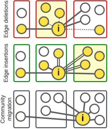
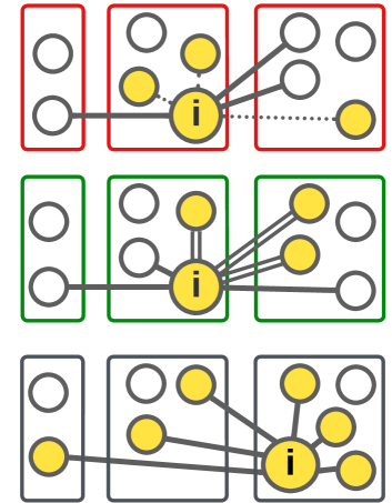
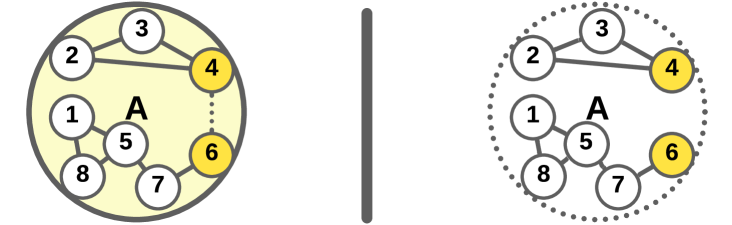
This dynamic community detection method employs modularity-based scoring to pinpoint regions of a graph where vertices may change their community membership. Zarayeneh et al. implement the DS approach by first sorting batch updates of edge deletions and insertions by source vertex ID. For edge deletions within the same community, they mark the neighbors of vertex and the community of vertex as affected. For edge insertions across communities, they identify vertex with the highest modularity change linked to vertex and mark the neighbors of and the community of as affected. Edge deletions between different communities and insertions within the same community are considered unlikely to influence community membership and are ignored. Figure 1(a) illustrates the affected vertices and communities related to a single source vertex in response to a batch update.
3.5.3. Dynamic Frontier (DF) approach (Sahu et al., 2024b)
This approach begins by initializing each vertex’s community membership based on the previous graph snapshot. When edges are deleted between vertices in the same community or inserted between different communities, the source vertex is marked as affected. Since batch updates are undirected, both endpoints and are marked. Edge deletions between different communities or insertions within the same community are ignored. Additionally, if vertex changes its community membership, all its neighboring vertices are marked as affected, while is marked as unaffected. To reduce unnecessary computations, an affected vertex is also marked as unaffected if its community remains unchanged. The DF approach then employs a graph traversal-like method until the community assignments stabilize. Figure 1(b) illustrates the vertices connected to a source vertex marked as affected by the DF approach after a batch update.
4. Approach
We now discuss techniques to address the two keys issues with the dynamic algorithms presented earlier by us (Sahu, 2024c), i.e., the stability of obtained communities, and performance.
4.1. Improving stability
Let us first consider addressing the issue of stability of obtained communities on dynamic graphs. Here, we are essentially asking the question of how well a dynamic community detection algorithm is able to help us keep track of the identified communities, by continuing to preserve the associated ID for each community across small updates, which modify the vertex set associated with the community, but do not significantly change it — or if they do, the change is slow, i.e., it appears over a number of batch updates.
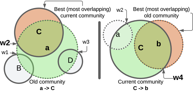
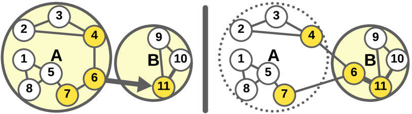
We propose the following procedure for tracking communities. It involves first identifying the most overlapping community (by total edge weight) to each old community in the previous graph snapshot, and then identifying the most overlapping old community to each current community (since a current community may be the best overlapping community for multiple old communities) — to create a mapping from each current community ID, , to the best matching old community ID, . Take a look at Figure 2 for an example. As shown in the left subfigure, we first identify that the current community is the most overlapping community with the old community (with a total overlap edge weight ). In the right subfigure, we observe that the current community has best overlaps with two old communities and , but since is the most overlapping old community (with a total overlap edge weight ), the final mapping created is from current community to old community . We use the Boyer-Moore majority vote algorithm (Boyer and Moore, 1991) in order to obtain the most (majority) overlapping community in a reasonable amount of time. We refer the reader to Section A.8 for more details.
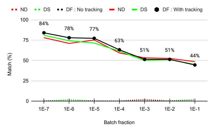
We now wish to measure the stability of communities identified with our proposed procedure, using ND, DS, and DF Leiden. For this, we consider the following experiment. First, we obtain the community membership of vertices in the initial snapshot of a graph , using Static Leiden. Next, we apply a random batch update, consisting purely of edge deletions, in order to obtain an updated graph . Here, we use each dynamic algorithm to obtain the updated community membership of vertices. Finally, we reinsert the same edges back to obtain the original graph , and reuse each dynamic algorithm to obtain the updated community membership of vertices from the membership obtained in . In the ideal case, the community memberships obtained by the dynamic algorithms on would have an exact match with the community memberships obtained by Static Leiden on . However, this is can be hard to achieve in practice. One of the reasons is that the refined communities may split off, and rejoin back, but will very likely not have the same community ID when they reform.
Figure 3 shows the percent match in the community membership of vertices with the original ND, DS, and DF Leiden (no tracking) (Sahu, 2024c), and our improved ND, DS, and DF Leiden (with tracking). For this experiment, we use graphs from Table 1, with the batch size being adjusted from to , and the arithmetic mean of the match percentage is plotted. As the figure shows, in the absence of tracking, ND, DS, and DF Leiden have a near zero match with the communities returned by Static Leiden of , and are thus not the right candidates for tracking evolving communities on dynamic graphs. In contrast, our improved ND, DS, and DF Leiden achieve a good match, with our improved DF Leiden achieving a match of to on batch updates of size to .
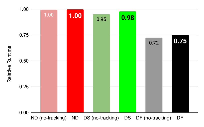
Next, we measure the runtime cost of the proposed procedure for tracking of communities — on large graphs, from Table 1, with randomly generated batch updates of size to . Figure 4 shows the relative runtime of the original ND, DS, and DF Leiden (no-tracking) (Sahu, 2024c), compared to our improved ND, DS, and DF Leiden. As the figure shows, the inclusion of the community tracking procedure incurs a minimal additional runtime overhead.
4.2. Minimizing communities to refine
We now focus on improving the speed of our dynamic algorithms. In particular, we note that once we refine a community, we must run the algorithm to the end. This means we should aim to minimize the number of communities that require refinement. Note that refinement offers us two key benefits: first, it ensures that we obtain well-connected communities without internal disconnections; second, it allows us to address edge cases, where an isolated community can independently split due to edge deletions or insertions. However, such edge case occurrences are relatively rare.
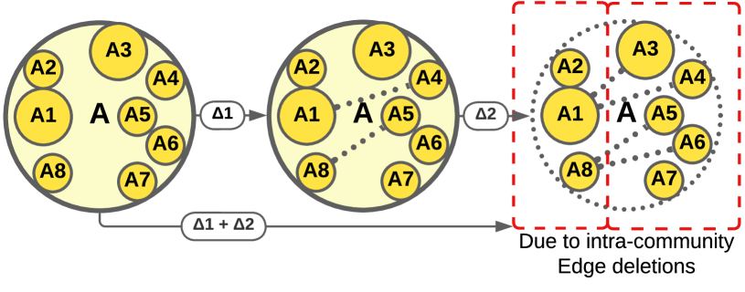
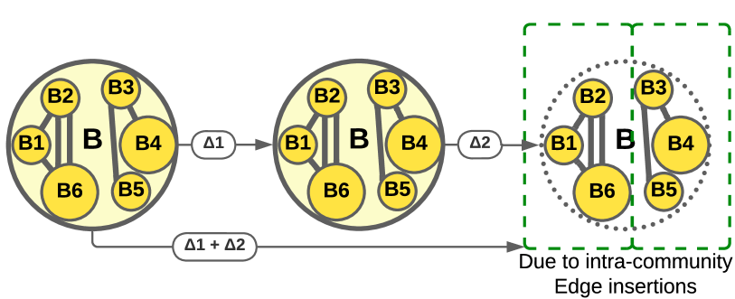
To optimize this process, we propose the following heuristic: we will mark a community for refinement only if the cumulative change in its total edge weight changes by a fraction greater than the refinement tolerance , considering both edge deletions and insertions as positive changes to community weight. Since the change in total edge weight of each community is aggregated until a community is marked for refinement, multiple sequential small batch updates have a similar effect as a single large batch update, as shown in Figure 5. When the change in total edge weight of a community exceeds this threshold, we mark it for refinement and reset the current total edge weight change for that community to zero. If no communities are marked for refinement, we can achieve convergence in a single pass, eliminating the need to run the algorithm till the end. The figure also shows how both edge deletions and edge insertions within a community may cause a community to split, and thus a community must be marked for refinement in both cases (to allow for subcommunities to be identified).
4.3. Minimizing communities to split
Now there still remains an issue. At no cost do we want to introduce disconnected communities in the returned community structures. Figure 7 shows two different cases which may cause a community to be internally-disconnected. First, as shown in the top subfigure, edge deletions within a community may cause it to become internally-disconnected. Therefore, during initialization, any community with intra-community edge deletions should be processed to split apart its disconnected components into separate communities. Second, as shown in the bottom subfigure, when a vertex migrates from its original community to another one — due to stronger connections — it can cause the original community to become internally disconnected. Thus, in the local-moving phase of the algorithm, source communities from which vertices migrate should also be processed to separate any disconnected components into distinct communities. Note however that if a community has already been marked for refinement, splitting is not necessary.
In order to address the above mentioned issues, we split all communities that are not being refined, at the end of each pass. This has been show to have better performance than simply splitting communities at the end of all passes (Sahu, 2024a). However, we can do better. We can identify a subset of communities to split, and ignore the communities that are guaranteed to have no disconnected communities. Note that a disconnected community may arise only for communities with intra-community edge deletions, and if a vertex migrates from its old community to some other community. Accordingly, we choose to keep track of such communities.
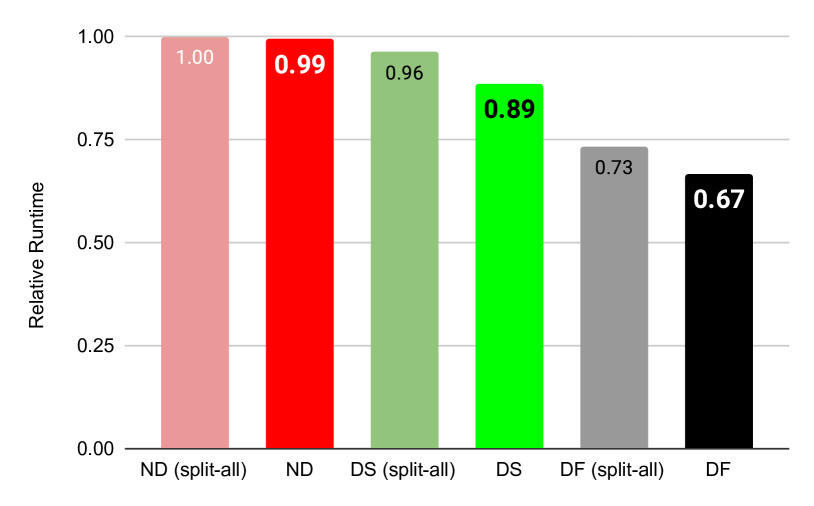
However, our initial observation seemed to indicate that tracking of communities to split has a relatively significant added cost. Accordingly, we conduct an experiment to measure the performance of ND, DS, and DF Leiden under two conditions: splitting all communities that have not been marked to be refined (”split-all”), and splitting only a subset of communities (which have a chance to form internally-disconnected communities), marked during initialization or the local-moving phase of the algorithm. We perform this experiment on large graphs with random batch updates of size ranging from to . Figure 8 shows the relative runtimes of ND, DS, and DF Leiden. As results show, splitting a subset of communities improves performance, despite added tracking cost.
4.4. Implementation details
We implement an asynchronous version of Leiden, allowing threads to independently process different graph sections, which enhances convergence speed but increases variability in results. Each thread maintains its own hashtable to track delta-modularity during local-moving and refinement phases, as well as total edge weights between super-vertices during aggregation. Optimizations include OpenMP’s dynamic loop scheduling, limiting iterations to 20 per pass, a tolerance drop rate of 10 starting at 0.01, vertex pruning, parallel prefix sums, and preallocated Compressed Sparse Row (CSR) structures for super-vertex graphs and community vertices, along with fast, collision-free per-thread hashtables (Sahu et al., 2024a). To ensure high-quality communities, we do not skip the aggregation phase of the algorithm (Sahu, 2024c), even when merging a small number of communities, unlike GVE-Leiden (Sahu et al., 2024a). This results in only a minor increase in runtime across Static, ND, DS, and DF Leiden. We also use a refine-based variation, where community labels of super-vertices are determined by the refinement instead of the local-moving phase, allowing for splitting apart of isolated communities.
The pseudocode for our improved ND, DS, and DF Leiden is given in Sections A.1, A.2 and A.3, respectively. During the first pass of the Leiden algorithm, we process the vertices identified as affected by the DS and DF approaches, initializing each vertex’s community membership based on the membership from the previous graph snapshot. In subsequent passes, all super-vertices are designated as affected and processed according to the Leiden algorithm (Sahu et al., 2024b). Similar to the DF Louvain method (Sahu, 2024b), we utilize the weighted degrees of vertices , the total edge weights of communities , and the cumulative change in the total edge weights of communities , as auxiliary information to the dynamic algorithm.
4.5. Time and Space complexity
The time complexity of ND, DS, and DF Leiden remains , similar to Static Leiden, where is the total number of iterations. However, the local-moving and refinement phases’ costs during the first pass are reduced and depend on the batch update’s size and nature. The space complexity matches that of Static Leiden, i.e., , with being the number of threads used ( accounts for per-thread collision-free hashtables (Sahu et al., 2024a)).
5. Evaluation
5.1. Experimental setup
5.1.1. System
We use a server with an x86-based 64-bit AMD EPYC-7742 processor running at GHz, paired with 512 GB of DDR4 RAM. Each core has a 4 MB L1 cache, a 32 MB L2 cache, and a shared 256 MB L3 cache. The server operates on Ubuntu 20.04.
5.1.2. Configuration
We use 32-bit unsigned integers for vertex IDs and 32-bit floating-point numbers for edge weights. For floating-point aggregations, we switch to 64-bit floating-point. Affected vertices and communities marked for splitting/refining are represented by 8-bit integer vectors. Key parameters include an iteration tolerance of for the local-moving phase, a refinement tolerance of , a TOLERANCE_DECLINE_FACTOR of for threshold scaling optimization (Lu et al., 2015), a MAX_ITERATIONS of for the local-moving phase per pass, and a MAX_PASSES of (Sahu et al., 2024a). We employ OpenMP’s dynamic scheduling with a chunk size of for the local-moving, refinement, and aggregation phases. However, for the aggregation phase in Naive-dynamic (ND), Delta-screening (DS), and Dynamic Frontier (DF) Leiden, we use a chunk size of for proper work balancing (Sahu, 2024c). We run all implementations on threads, unless stated otherwise, and compile using GCC 9.4 with OpenMP 5.0.
5.1.3. Dataset
We conduct experiments on large real-world graphs with random batch updates, as listed in Table 1, sourced from the SuiteSparse Matrix Collection. These graphs range in size from million to million vertices, and from million to billion edges. For experiments involving real-world dynamic graphs, we utilize five temporal networks from the Stanford Large Network Dataset Collection (Leskovec and Krevl, 2014), detailed in Table 2. These networks feature vertex counts between thousand and million, with temporal edges ranging from thousand to million, and static edges from thousand to million. However, it is worth noting that most temporal graphs in the SNAP repository (Leskovec and Krevl, 2014) are relatively small, limiting their applicability for studying our proposed parallel algorithms. In all experiments, we ensure that the edges are undirected and weighted, with a default weight of . Due to the small size of most publicly available real-world weighted graphs, we do not use them in this study, although our parallel algorithms can handle weighted graphs without modification.
Additionally, we exclude SNAP datasets with ground-truth communities because they are non-disjoint, while our focus is on disjoint communities. It is important to note that community detection is not solely about matching ground truth, as this may not accurately represent the network’s actual structure and could overlook meaningful community patterns (Peel et al., 2017).
5.1.4. Batch generation
We take each base graph from Table 1 and generate random batch updates (Zarayeneh and Kalyanaraman, 2021) with an mix of edge insertions and deletions, each edge weighted at . All updates are undirected; for each insertion , we also include . Vertex pairs are selected uniformly for insertions, while existing edges are uniformly deleted for deletions. No new vertices are added or removed. The batch size, measured as a fraction of the original graph’s edges, ranges from to , translating to to million edges for a billion-edge graph. We conduct five distinct random batch updates for each batch size and report the average results. Do note that dynamic graph algorithms are useful for small batch updates, such as in interactive applications, while static algorithms are generally more efficient for larger batches.
For experiments on real-world dynamic graphs, we initially load of each graph listed in Table 2. As earlier, all edges are assigned a default weight of and are made undirected by adding their reverse edges. Next, we load edges for batch updates, where represents the batch size as a fraction of the total temporal edges, , in the graph. Each batch update is ensured to be undirected.
| Graph | |||
|---|---|---|---|
| Web Graphs (LAW) | |||
| indochina-2004∗ | 7.41M | 341M | 2.68K |
| arabic-2005∗ | 22.7M | 1.21B | 2.92K |
| uk-2005∗ | 39.5M | 1.73B | 18.2K |
| webbase-2001∗ | 118M | 1.89B | 2.94M |
| it-2004∗ | 41.3M | 2.19B | 4.05K |
| sk-2005∗ | 50.6M | 3.80B | 2.67K |
| Social Networks (SNAP) | |||
| com-LiveJournal | 4.00M | 69.4M | 3.09K |
| com-Orkut | 3.07M | 234M | 36 |
| Road Networks (DIMACS10) | |||
| asia_osm | 12.0M | 25.4M | 2.70K |
| europe_osm | 50.9M | 108M | 6.13K |
| Protein k-mer Graphs (GenBank) | |||
| kmer_A2a | 171M | 361M | 21.1K |
| kmer_V1r | 214M | 465M | 10.5K |
| Graph | |||
|---|---|---|---|
| sx-mathoverflow | 24.8K | 507K | 240K |
| sx-askubuntu | 159K | 964K | 597K |
| sx-superuser | 194K | 1.44M | 925K |
| wiki-talk-temporal | 1.14M | 7.83M | 3.31M |
| sx-stackoverflow | 2.60M | 63.4M | 36.2M |
5.1.5. Measurement
We assess the runtime of each method on the entire updated graph, covering all phases of the algorithm. To minimize the impact of noise in our experiments, we adhere to the standard practice of running each experiment multiple times. We assume the total edge weight of the graphs is known and can be tracked with each batch update. As a baseline, we use the most efficient multicore implementation of Static Leiden, GVE-Leiden (Sahu et al., 2024a), which has been shown to outperform even GPU-based approaches. Since modularity maximization is NP-hard and all existing polynomial-time algorithms are heuristic-based, we evaluate the optimality of our dynamic algorithms by comparing their convergence to the modularity score achieved by the static algorithm. Finally, because none of the algorithms analyzed — Static, ND, DS, and DF Leiden — produce internally disconnected communities, we omit this detail from our figures.
5.2. Performance comparison
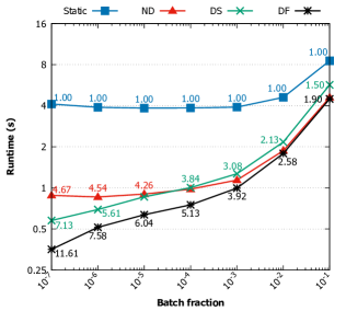
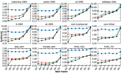
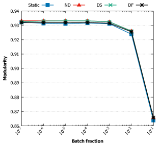
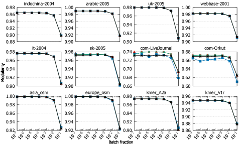
We now measure the performance of parallel implementations of our improved ND, DS, and DF Leiden against Static Leiden (Sahu et al., 2024a) on large graphs, given in Table 1, with randomly generated batch updates. As outlined in Section 5.1.4, these updates vary in size from to , with edge insertions and edge deletions. Each batch update includes reverse edges to maintain an undirected graph structure. Figure 9(b) illustrates the execution time of each algorithm for individual graphs, while Figure 9(a) provides a comparison of overall runtimes using the geometric mean for consistent scaling across different graph sizes. Additionally, Figure 10(b) presents the modularity results for each graph in the dataset, and Figure 10(a) shows the overall modularity for each algorithm, averaged using the arithmetic mean. Performance comparison on real-world dynamic graphs from Table 2 is given in Section A.9.
From Figure 9(a), we can see that our improved ND, DS, and DF Leiden achieve mean speedups of , , and , respectively, compared to Static Leiden. These speedups are even more pronounced for smaller batch updates, where ND, DS, and DF Leiden provide average speedups of , , and , respectively, for batch updates of size . Figure 9(b) further illustrates that ND, DS, and DF Leiden deliver significant speedups across all graph types, though the gains are somewhat lower for social networks (with high average degree nodes) and protein k-mer graphs (with low average degree nodes). This may be due to these classes of graphs lacking dense community structures.
In terms of modularity, as shown in Figures 10(a) and 10(b), our improved ND, DS, and DF Leiden achieve communities with modularity scores comparable to those of Static Leiden. However, on social networks, ND, DS, and DF Leiden slightly outperform Static Leiden. This is likely because social networks lack a strong community structure and thus require more iterations to reach a good community assignment. On these graphs, Static Leiden tends to underperform in terms of modularity due to its constraint on the number of iterations per pass, which is designed to prioritize faster runtimes. In contrast, ND, DS, and DF Leiden, which build upon the community membership generated by Static Leiden rather than starting from scratch, are able to refine and improve the modularity. Nonetheless, the difference in modularity between Static Leiden and our algorithms is less than on average.
Additionally, note in Figure 9 that the runtime of Static Leiden increases with larger batch updates. This is mainly because random batch updates disrupt the existing community structure, requiring Static Leiden to perform more iterations to reach convergence — it is not solely a consequence of the graph’s increased edge count. This disruption also explains the observed decrease in modularity for all algorithms as batch sizes grow, as seen in Figure 10.
5.3. Affected vertices and Marked communities
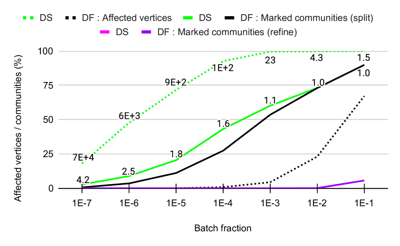
We now analyze the fraction of vertices marked as affected, the fraction of communities marked for splitting, and the fraction of communities marked for refinement by our improved DS and DF Leiden algorithms. This analysis is conducted over the instances in Table 1, using batch updates ranging from to . It is important to note that we only track affected vertices and marked communities (for splitting and refinement) during the first pass of the Leiden algorithm. These results are presented in Figure 11.
From Figure 11, we observe that DF Leiden marks significantly fewer vertices as affected compared to DS Leiden. However, the runtime difference between the two algorithms is smaller, as many of the vertices marked by DS Leiden do not change their community labels and converge quickly. Additionally, the number of affected vertices does not fully account for the overall performance differences between the two algorithms. The figure also shows that DF Leiden marks fewer communities for splitting than DS Leiden, though the gap is much smaller than that of affected vertices, and more closely mirrors the performance gap between DS and DF Leiden. Finally, both DS and DF Leiden mark roughly the same small fraction of communities for refinement, thanks to our heuristic that minimizes the number of communities to be refined. This fraction only becomes noticeable at a batch size of . As expected, performance deteriorates with an increasing number of affected vertices and marked communities, as shown in Figures 9 and 11. While a high number of marked communities increases splitting and refinement costs in the first pass, the cost of subsequent passes depends primarily on the nature of the graph.
5.4. Scalability
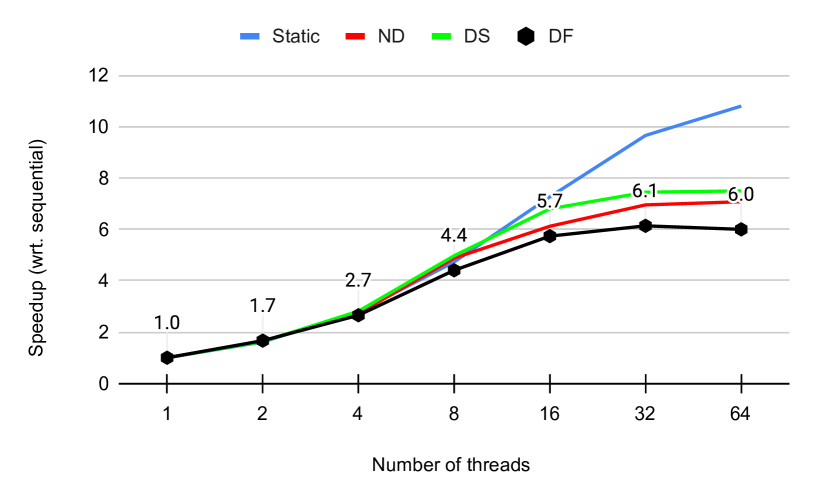
Finally, we study the strong-scaling behavior of our improved ND, DS, and DF Leiden, and compare to Static Leiden. For this, we fix the batch size at and vary thread count from to , measuring the speedup of each algorithm relative to its sequential execution.
As shown in Figure 12, at threads, ND, DS, and DF Leiden achieve speedups of , , and , respectively, compared to their sequential counterparts. Their speedups increase at average rates of , , and for every doubling of thread count. However, at threads, performance is impacted by NUMA effects. Additionally, as thread count increases, the algorithms behave more synchronously — similar to the Jacobi iterative method — further reducing performance. The limited scalability is also due to the presence of sequential steps in the algorithms and insufficient work to distribute across threads for the dynamic algorithms.
6. Conclusion
This technical report introduced three techniques/heuristics aimed at enhancing the performance and stability of our previously proposed multicore dynamic community detection algorithms based on Leiden (Sahu, 2024c). Experiments conducted on a 64-core AMD EPYC-7742 processor show that our improved ND, DS, and DF Leiden algorithms achieve average speedups of , , and , respectively, on large graphs undergoing random batch updates when compared to the Static Leiden algorithm. Additionally, these methods demonstrate a scaling efficiency of for each doubling of threads. In the future, we would like to further improve the trackability of communities on evolving graphs.
Acknowledgements.
I would like to thank Prof. Kishore Kothapalli and Prof. Dip Sankar Banerjee for their support.References
- (1)
- Aktunc et al. (2015) R. Aktunc, I. Toroslu, M. Ozer, and H. Davulcu. 2015. A dynamic modularity based community detection algorithm for large-scale networks: DSLM. In Proceedings of the IEEE/ACM international conference on advances in social networks analysis and mining. 1177–1183.
- Aynaud and Guillaume (2010) T. Aynaud and J. Guillaume. 2010. Static community detection algorithms for evolving networks. In 8th International Symposium on Modeling and Optimization in Mobile, Ad Hoc, and Wireless Networks. IEEE, IEEE, Avignon, France, 513–519.
- Bai et al. (2024) Yuhe Bai, Camelia Constantin, and Hubert Naacke. 2024. Leiden-Fusion Partitioning Method for Effective Distributed Training of Graph Embeddings. In Joint European Conference on Machine Learning and Knowledge Discovery in Databases. Springer, 366–382.
- Blekanov et al. (2021) Ivan Blekanov, Svetlana S Bodrunova, and Askar Akhmetov. 2021. Detection of hidden communities in twitter discussions of varying volumes. Future Internet 13, 11 (2021), 295.
- Blondel et al. (2008) V. Blondel, J. Guillaume, R. Lambiotte, and E. Lefebvre. 2008. Fast unfolding of communities in large networks. Journal of Statistical Mechanics: Theory and Experiment 2008, 10 (Oct 2008), P10008.
- Boyer and Moore (1991) Robert S Boyer and J Strother Moore. 1991. MJRTY—a fast majority vote algorithm. In Automated reasoning: essays in honor of Woody Bledsoe. Springer, 105–117.
- Brandes et al. (2007) U. Brandes, D. Delling, M. Gaertler, R. Gorke, M. Hoefer, Z. Nikoloski, and D. Wagner. 2007. On modularity clustering. IEEE transactions on knowledge and data engineering 20, 2 (2007), 172–188.
- Cao and Zhang (2022) Lingli Cao and Cheng Zhang. 2022. Implementation of domain-oriented microservices decomposition based on node-attributed network. In Proceedings of the 2022 11th International Conference on Software and Computer Applications. 136–142.
- Chen et al. (2023) Wendong Chen, Xize Liu, Xuewu Chen, Long Cheng, and Jingxu Chen. 2023. Deciphering flow clusters from large-scale free-floating bike sharing journey data: a two-stage flow clustering method. Transportation (2023), 1–30.
- Chernikova et al. (2022) Alesia Chernikova, Nicolò Gozzi, Simona Boboila, Priyanka Angadi, John Loughner, Matthew Wilden, Nicola Perra, Tina Eliassi-Rad, and Alina Oprea. 2022. Cyber network resilience against self-propagating malware attacks. In European Symposium on Research in Computer Security. Springer, 531–550.
- Chong and Teow (2013) W. Chong and L. Teow. 2013. An incremental batch technique for community detection. In Proceedings of the 16th International Conference on Information Fusion. IEEE, IEEE, Istanbul, Turkey, 750–757.
- Cordeiro et al. (2016) M. Cordeiro, R. Sarmento, and J. Gama. 2016. Dynamic community detection in evolving networks using locality modularity optimization. Social Network Analysis and Mining 6, 1 (2016), 1–20.
- Desvars-Larrive et al. (2024) Amélie Desvars-Larrive, Anna Elisabeth Vogl, Gavrila Amadea Puspitarani, Liuhuaying Yang, Anja Joachim, and Annemarie Käsbohrer. 2024. A One Health framework for exploring zoonotic interactions demonstrated through a case study. Nature communications 15, 1 (2024), 5650.
- Erfan et al. (2023) Fatemeh Erfan, Martine Bellaiche, and Talal Halabi. 2023. Community detection algorithm for mitigating eclipse attacks on blockchain-enabled metaverse. In 2023 IEEE International Conference on Metaverse Computing, Networking and Applications (MetaCom). IEEE, 403–407.
- Ghoshal et al. (2019) A. Ghoshal, N. Das, S. Bhattacharjee, and G. Chakraborty. 2019. A fast parallel genetic algorithm based approach for community detection in large networks. In 11th International Conference on Communication Systems & Networks (COMSNETS). IEEE, Bangalore, India, 95–101.
- Gregory (2010) S. Gregory. 2010. Finding overlapping communities in networks by label propagation. New Journal of Physics 12 (10 2010), 103018. Issue 10.
- Hartman et al. (2024) Erik Hartman, Fredrik Forsberg, Sven Kjellström, Jitka Petrlova, Congyu Luo, Aaron Scott, Manoj Puthia, Johan Malmström, and Artur Schmidtchen. 2024. Peptide clustering enhances large-scale analyses and reveals proteolytic signatures in mass spectrometry data. Nature Communications 15, 1 (2024), 7128.
- Held et al. (2016) P. Held, B. Krause, and R. Kruse. 2016. Dynamic clustering in social networks using louvain and infomap method. In Third European Network Intelligence Conference (ENIC). IEEE, IEEE, Wroclaw, Poland, 61–68.
- Heumos et al. (2023) Lukas Heumos, Anna C Schaar, Christopher Lance, Anastasia Litinetskaya, Felix Drost, Luke Zappia, Malte D Lücken, Daniel C Strobl, Juan Henao, Fabiola Curion, et al. 2023. Best practices for single-cell analysis across modalities. Nature Reviews Genetics 24, 8 (2023), 550–572.
- Kapoor et al. (2021) Arnav Kapoor, Rishi Raj Jain, Avinash Prabhu, Tanvi Karandikar, and Ponnurangam Kumaraguru. 2021. “I’ll be back”: Examining Restored Accounts On Twitter. In IEEE/WIC/ACM International Conference on Web Intelligence and Intelligent Agent Technology. 71–78.
- Kolodziej et al. (2019) S. Kolodziej, M. Aznaveh, M. Bullock, J. David, T. Davis, M. Henderson, Y. Hu, and R. Sandstrom. 2019. The SuiteSparse matrix collection website interface. JOSS 4, 35 (Mar 2019), 1244.
- La Cava et al. (2022) Lucio La Cava, Sergio Greco, and Andrea Tagarelli. 2022. Information consumption and boundary spanning in decentralized online social networks: the case of mastodon users. Online Social Networks and Media 30 (2022), 100220.
- La Morgia et al. (2021) Massimo La Morgia, Alessandro Mei, Alberto Maria Mongardini, and Jie Wu. 2021. Uncovering the dark side of Telegram: Fakes, clones, scams, and conspiracy movements. arXiv preprint arXiv:2111.13530 (2021).
- Lancichinetti and Fortunato (2009) A. Lancichinetti and S. Fortunato. 2009. Community detection algorithms: a comparative analysis. Physical Review. E, Statistical, Nonlinear, and Soft Matter Physics 80, 5 Pt 2 (Nov 2009), 056117.
- Leskovec and Krevl (2014) Jure Leskovec and Andrej Krevl. 2014. SNAP Datasets: Stanford Large Network Dataset Collection. http://snap.stanford.edu/data.
- Liu et al. (2024) Zhenze Liu, Yingjian Liang, Guohua Wang, and Tianjiao Zhang. 2024. scLEGA: an attention-based deep clustering method with a tendency for low expression of genes on single-cell RNA-seq data. Briefings in Bioinformatics 25, 5 (2024).
- Lu et al. (2015) Hao Lu, Mahantesh Halappanavar, and Ananth Kalyanaraman. 2015. Parallel heuristics for scalable community detection. Parallel Comput. 47 (2015), 19–37.
- Meng et al. (2016) X. Meng, Y. Tong, X. Liu, S. Zhao, X. Yang, and S. Tan. 2016. A novel dynamic community detection algorithm based on modularity optimization. In 7th IEEE international conference on software engineering and service science (ICSESS). IEEE, IEEE, Beijing,China, 72–75.
- Müller-Bötticher et al. (2024) Niklas Müller-Bötticher, Shashwat Sahay, Roland Eils, and Naveed Ishaque. 2024. SpatialLeiden-Spatially-aware Leiden clustering. bioRxiv (2024), 2024–08.
- Newman (2004) M. Newman. 2004. Detecting community structure in networks. The European Physical Journal B - Condensed Matter 38, 2 (Mar 2004), 321–330.
- Newman and Reinert (2016) M. Newman and G. Reinert. 2016. Estimating the number of communities in a network. Physical review letters 117, 7 (2016), 078301.
- Peel et al. (2017) Leto Peel, Daniel B Larremore, and Aaron Clauset. 2017. The ground truth about metadata and community detection in networks. Science advances 3, 5 (2017), e1602548.
- Raghavan et al. (2007) U. Raghavan, R. Albert, and S. Kumara. 2007. Near linear time algorithm to detect community structures in large-scale networks. Physical Review E 76, 3 (Sep 2007), 036106–1–036106–11.
- Sahu (2024a) Subhajit Sahu. 2024a. An Approach for Addressing Internally-Disconnected Communities in Louvain Algorithm. arXiv preprint arXiv:2402.11454 (2024).
- Sahu (2024b) Subhajit Sahu. 2024b. DF Louvain: Fast Incrementally Expanding Approach for Community Detection on Dynamic Graphs. arXiv preprint arXiv:2404.19634 (2024).
- Sahu (2024c) Subhajit Sahu. 2024c. A Starting Point for Dynamic Community Detection with Leiden Algorithm. arXiv preprint arXiv:2405.11658 (2024).
- Sahu et al. (2024a) Subhajit Sahu, Kishore Kothapalli, and Dip Sankar Banerjee. 2024a. Fast Leiden Algorithm for Community Detection in Shared Memory Setting. In Proceedings of the 53rd International Conference on Parallel Processing. 11–20.
- Sahu et al. (2024b) Subhajit Sahu, Kishore Kothapalli, and Dip Sankar Banerjee. 2024b. Shared-Memory Parallel Algorithms for Community Detection in Dynamic Graphs. In 2024 IEEE International Parallel and Distributed Processing Symposium Workshops (IPDPSW). IEEE, 250–259.
- Shang et al. (2014) J. Shang, L. Liu, F. Xie, Z. Chen, J. Miao, X. Fang, and C. Wu. 2014. A real-time detecting algorithm for tracking community structure of dynamic networks.
- Sliwa et al. (2024) Karolina Sliwa, Ema Kusen, and Mark Strembeck. 2024. A Case Study Comparing Twitter Communities Detected by the Louvain and Leiden Algorithms During the 2022 War in Ukraine. In Companion Proceedings of the ACM on Web Conference 2024. 1376–1381.
- Traag et al. (2019) V. Traag, L. Waltman, and N. Eck. 2019. From Louvain to Leiden: guaranteeing well-connected communities. Scientific Reports 9, 1 (Mar 2019), 5233.
- Uyheng et al. (2021) Joshua Uyheng, Aman Tyagi, and Kathleen M Carley. 2021. Mainstream consensus and the expansive fringe: characterizing the polarized information ecosystems of online climate change discourse. In Proceedings of the 13th ACM Web Science Conference 2021. 196–204.
- Verhetsel et al. (2022) Ann Verhetsel, Joris Beckers, and Jeroen Cant. 2022. Regional retail landscapes emerging from spatial network analysis. Regional Studies 56, 11 (2022), 1829–1844.
- Wang et al. (2021) Changzhen Wang, Fahui Wang, and Tracy Onega. 2021. Network optimization approach to delineating health care service areas: Spatially constrained Louvain and Leiden algorithms. Transactions in GIS 25, 2 (2021), 1065–1081.
- Yin et al. (2016) S. Yin, S. Chen, Z. Feng, K. Huang, D. He, P. Zhao, and M. Yang. 2016. Node-grained incremental community detection for streaming networks. In IEEE 28th International Conference on Tools with Artificial Intelligence (ICTAI). IEEE, 585–592.
- Zang et al. (2023) Xiaodong Zang, Jian Gong, Xinchang Zhang, and Guiqing Li. 2023. Attack scenario reconstruction via fusing heterogeneous threat intelligence. Computers & Security 133 (2023), 103420.
- Zarayeneh and Kalyanaraman (2021) N. Zarayeneh and A. Kalyanaraman. 2021. Delta-Screening: A Fast and Efficient Technique to Update Communities in Dynamic Graphs. IEEE transactions on network science and engineering 8, 2 (Apr 2021), 1614–1629.
- Zhou et al. (2023) Naitian Zhou, David Jurgens, and David Bamman. 2023. Social Meme-ing: Measuring Linguistic Variation in Memes. arXiv preprint arXiv:2311.09130 (2023).
- Zhuang et al. (2019) D. Zhuang, J. Chang, and M. Li. 2019. DynaMo: Dynamic community detection by incrementally maximizing modularity. IEEE Transactions on Knowledge and Data Engineering 33, 5 (2019), 1934–1945.
Appendix A Appendix
A.1. Our Parallel Naive-dynamic (ND) Leiden
Algorithm 1 presents a multicore implementation of our improved ND Leiden, where vertices are assigned to communities based on the previous graph snapshot. All vertices are processed, regardless of edge deletions or insertions, but the algorithm identifies specific communities that need to be split or refined based on the batch update. It takes as input the current graph snapshot , edge deletions , insertions in the batch update, previous community memberships , vertex weighted degrees , total community edge weights , and their changes . It returns the updated community memberships , vertex weighted degrees , and community edge weights with their changes .
In the algorithm, two lambda functions, isAffected() (lines 14-15) and inAffectedRange() (lines 16-17), are defined. These functions indicate that all vertices in the graph should be marked as affected and that these vertices can be incrementally marked as affected, respectively. We then use , , along with the batch updates and , to quickly compute and , which are required for the local-moving phase of the Leiden algorithm (line 20). We also utilize the batch update to quickly update to , which is used to keep track of the cumulative change in total edge weight of each community (line 21). This is used, along with the batch update, to identify the communities that need to be refined, in , as well as the communities that need to be split, in (line 23). These are then employed to run the Leiden algorithm and obtain the updated communities (line 25). Finally, is returned, along with , , and as the updated auxiliary information (line 26).
A.2. Our Parallel Delta-screening (DS) Leiden
Algorithm 2 outlines the pseudocode for multicore implementation of our improved DS Leiden. It uses modularity-based scoring to identify areas of the graph where community membership of vertices is likely to change (Zarayeneh and Kalyanaraman, 2021). Input includes the current graph snapshot , edge deletions and insertions from the batch update, previous community memberships , weighted vertex degrees , total community edge weights , and the changes in their total edge weights . The output consists of updated community memberships , weighted degrees , total community edge weights , and changes in the total edge weights . Before processing, edge deletions and insertions are sorted separately by source vertex ID .
In the algorithm, we begin by initializing a hashtable that maps communities to their corresponding weights. We also set the affected flags , , and , which indicate whether a vertex, its neighbors, or its community is impacted by the batch update (lines 15). Edge deletions and insertions are then processed in parallel. For each deletion , where vertices and are in the same community, we mark the source vertex , its neighbors, and its community as affected (lines 17-19). For each unique source vertex in the insertions , if and belong to different communities, we identify the community that maximizes the delta-modularity if were to move to one of its neighboring communities. We then mark , its neighbors, and the community as affected (lines 20-26). Deletions between different communities and insertions within the same community are ignored. Using the affected neighbors and community flags , we update the affected vertices in (lines 27-32). Next, similar to ND Leiden, we use and , along with and , to efficiently compute and (line 39). Additionally, we leverage the batch update to quickly adjust to , which tracks the cumulative change in the total edge weight of each community (line 40). This information, combined with the batch update, helps identify the communities that require refinement, in , and those that need to be split, in (line 42). We then define the necessary lambda functions, isAffected() (lines 33-34) and inAffectedRange() (lines 35-36), and run the Leiden algorithm to produce updated community assignments (line 44). Finally, we return updated community memberships along with , , and as updated auxiliary data (line 45).
A.3. Our Parallel Dynamic Frontier (DF) Leiden
Algorithm 3 outlines the pseudocode for our improved parallel DF Leiden implementation. The input includes the updated graph snapshot , edge deletions and insertions in the batch update, the previous community assignments for each vertex, weighted degrees of vertices, total edge weights of communities, and the change in total edge weights of communities. The algorithm produces the updated community memberships , weighted degrees of vertices, total edge weights , and the change in total edge weights of communities.
In the algorithm, we begin by identifying a set of affected vertices whose community memberships might change due to batch updates. These vertices are marked in the flag vector . Specifically, we mark the endpoints of deleted edges that belong to the same community (lines 16-17), as well as the endpoints of inserted edges that connect vertices from different communities (lines 18-19). Next, three lambda functions are defined for the Leiden algorithm: isAffected() (lines 20-21), inAffectedRange() (lines 22-23), and onChange() (lines 24-25). These functions define how vertices are marked as affected: initially through the batch update, incrementally during graph traversal, and when a vertex changes its community, respectively. Importantly, the set of affected vertices grows automatically due to the vertex pruning optimization used in our Parallel Leiden algorithm (Algorithm 4). Here, onChange() simulates the effect of a plain DF approach without pruning. Our approach leverages the previous state of the graph, and , alongside the batch updates and , to efficiently compute the new states and , which are essential for the local-moving phase of the Leiden algorithm (line 28). We also use the batch update to quickly update to , which tracks the cumulative change in each community’s total edge weight (line 29). This information, together with the batch update, helps us identify the communities that require refinement in and those that need to be split in (line 31). The lambda functions are then employed to execute the Leiden algorithm and generate the updated community assignments, (line 33). Finally, we return , along with , , and as the updated auxiliary information (line 34).
A.4. Our Dynamic-supporting Parallel Leiden
The main step of our Dynamic-supporting Parallel Leiden is presented in Algorithm 4. Unlike our Static Leiden implementation (Sahu et al., 2024a), this algorithm takes into account not only the current graph snapshot but also the previous community memberships of each vertex, the updated weighted degree of each vertex, the updated total edge weight of each community, and the change in total edge weight of each community. Additionally, it accepts flag vectors and , which indicate whether a community should be split or refined, along with a set of lambda functions that determine if a vertex is affected or can be progressively identified as affected within the affected range. Finally, updated community memberships of vertices, denoted as , are returned.
The algorithm begins by marking the affected vertices as unprocessed (lines 17-18), and initializing the community membership for each vertex in , among others. Once initialization is complete, a series of passes are conducted, limited by . Each pass consists of local-moving, splitting, refinement, and aggregation phases (lines 23-38). In each pass, the Leiden algorithm’s local-moving phase (Algorithm 6) is executed on the affected (unprocessed) vertices to optimize community assignments while identifying communities that may require splitting, recorded in (line 24). Communities identified in that have not been marked for refinement are then split to prevent the emergence of disconnected communities (line 26). This process involves renumbering the communities by the ID of a vertex within each community using the leidenSubsetRename() function (line 25). Renumbering is crucial since only a subset of communities will be split or refined, and using the ID of a contained vertex helps avoid two disconnected communities from sharing the same ID. The total edge weights of communities and the flags for communities to be split and refined in and are updated accordingly. Next, the identified communities for refinement in undergo the refinement phase, executed by leidenRefine(). This phase optimizes the community assignments for each vertex within their respective community boundaries obtained from the local-moving phase (line 28). If the local-moving phase converged after a single iteration during the first pass or if no communities were refined, convergence is achieved, and the community detection process halts (line 30). Conversely, if convergence is not reached, the aggregation phase is initiated. This phase includes renumbering the communities, updating the top-level community memberships using a dendrogram lookup, performing the aggregation process (Algorithm 9), and updating the weighted degrees of vertices and total edge weights of communities in the super-vertex graph. To prepare for the next pass, all vertices in the graph are marked as unprocessed, community memberships are initialized based on the refinement phase, all communities are marked for refinement for the upcoming pass, and the convergence threshold is adjusted by scaling (line 38). The next pass then begins (line 23). After completing all passes, the top-level community memberships for each vertex in are updated through dendrogram lookup (lines 39-41). This information is subsequently fed into the community tracking algorithm, leidenTrack(), which facilitates tracking communities even after they have been renumbered due to splits or refinements. Finally, the updated community memberships are returned.
A.4.1. Local-moving phase of our Parallel Leiden
The pseudocode for the local-moving phase of our Parallel Leiden algorithm is outlined in Algorithm 6. This phase iteratively moves vertices between communities in order to maximize modularity. Here, the leidenMove() function takes the current graph , community membership , total edge weight of each vertex, total edge weight of each community, a flag vector for communities marked to be split, and a set of lambda functions as inputs, and ultimately returns the number of iterations executed .
Lines 12-26 outline the core loop of the local-moving phase. In line 13, we initialize the total delta-modularity for each iteration, denoted as . Then, in lines 14-25, we iterate concurrently over unprocessed vertices. For each vertex , we execute vertex pruning by marking it as processed (line 15). We then check whether is within the affected range (i.e., it can be incrementally marked as affected). If it is not, we move on to the next vertex (line 16). For each vertex that is not skipped, we scan the communities connected to it (line 17), excluding itself, to identify the optimal community for moving to (line 19). We then compute the delta-modularity for this potential move (line 20), update the community membership of (lines 22-23), and mark its neighbors as unprocessed (line 24) if a better community is found. Additionally, for ND, DS, and DF Leiden, we designate the source community of the migrating vertex as a candidate community to be split in . In the case of Static Leiden, all communities are refined, and thus do not require splitting. In line 26, we check for convergence of the local-moving phase; if convergence is achieved or if the maximum number of iterations is reached, the loop terminates. Finally, in line 27, we return the total number of iterations performed, denoted as .
A.4.2. Splitting phase of our Parallel Leiden
Next, we will outline the pseudocode for the splitting phase, as detailed in Algorithm 7. This phase employs a parallel Breadth First Search (BFS) technique to partition disconnected communities. The function leidenSplit() takes as input the graph for the current pass, the community membership for each vertex, and the flag vectors and , which indicate whether each community is marked for splitting or refining. It returns the updated community membership for each vertex, where all the disconnected communities have been split into separate communities.
At the outset, lines 11-15 initialize the flag vector , which indicates whether vertices have been visited, the flag vector , which shows if a community is currently under processing by a thread, and the labels for each vertex, which are set to their respective vertex IDs. Following this, each thread processes every vertex in the graph concurrently (lines 17-24). If vertex has already been visited, or if the community associated with vertex is marked as busy (i.e., being processed by another thread), the current thread skips to the next iteration (line 19). On the other hand, if vertex has not been visited and community is not busy, the thread attempts to mark community as busy using (line 20). If this attempt fails, the thread proceeds to the next iteration. However, if the marking is successful, a BFS is initiated from vertex to explore the vertices within the same community. This BFS employs lambda functions: to selectively execute BFS on vertex if it belongs to the same community, and to update the labels of visited vertices after exploring each vertex during the BFS (line 23). Once all vertices have been processed, the threads synchronize, returning the updated labels , which reflect the new community membership of each vertex without any disconnected communities (line 25). Finally, community is marked as not busy, allowing it to be processed by other threads. At the end of the algorithm, the updated community membership is returned.
A.4.3. Refinement phase of our Parallel Leiden
The pseudocode for the refinement phase of our Parallel Leiden algorithm is detailed in Algorithm 6. This phase closely resembles the local-moving phase but includes the community membership assigned to each vertex as a community bound. During this phase, each vertex must choose a community within its community bound to join, with the goal of maximizing modularity through iterative movements between communities, similar to the local-moving phase. At the start of the refinement phase, the community membership of each vertex is reset, so that each vertex initially represents its own community. The leidenRefine() function is utilized, which takes the current graph , the community bound for each vertex , the initial community membership for each vertex, the total edge weight for each vertex , the initial total edge weight for each community , a flag vector that indicates which communities are to be refined, and the current tolerance per iteration as inputs.
The algorithm begins by breaking apart communities that have been marked for refinement in . It does this by resetting the community memberships of vertices, such that each vertex initially belongs to its own individual community. Following this, we implement the constrained merge procedure, as described in (Traag et al., 2019), during lines 14-24. This procedure allows vertices within each community boundary to form sub-communities by permitting only isolated vertices (those that belong solely to their own community) to change their community affiliation. This approach effectively divides any internally disconnected communities identified in the local-moving phase and prevents the formation of new disconnected communities. For each isolated vertex (line 16), we determine the communities connected to within the same community boundary, excluding itself (line 17). The refinement phase is skipped for a vertex if its community has not been marked for refinement () or if another vertex has joined its community, which is indicated by the total community weight no longer aligning with the total edge weight of the vertex. Next, we identify the optimal community for relocating (line 19) and evaluate the delta-modularity of moving to (line 20). If a better community is found, we attempt to update the community membership of , provided that it is still isolated (lines 22-24). We do not migrate vertex to community if the vertex representing has moved to a different community.
A.4.4. Aggregation phase of our Parallel Leiden
The pseudocode for the aggregation phase is detailed in Algorithm 9, where communities are combined into super-vertices. In particular, the leidenAggre gate() function of this algorithm accepts the current graph and the community membership of vertices in the current pass as inputs, and returns the super-vertex graph as output.
In the algorithm, the process begins by obtaining the offsets array for the community vertices in the CSR format, referred to as , as detailed in lines 10 to 11. This involves counting the number of vertices in each community using the function countCommunityVertices(), followed by performing an exclusive scan on the resulting array. Next, in lines 12 to 13, we concurrently traverse all vertices and atomically assign the vertices associated with each community into the community graph CSR . Subsequently, the offsets array for the super-vertex graph CSR is computed by estimating the degree of each super-vertex in lines 15 to 16. This includes calculating the total degree of each community using communityTotalDegree() and executing another exclusive scan. As a result, the super-vertex graph CSR is structured with intervals for the edges and weights array of each super-vertex. Then, in lines 18 to 24, we iterate over all communities in parallel, utilizing dynamic loop scheduling with a chunk size of for Static Leiden, and a chunk size of for ND, DS, and DF Leiden. During this stage, all communities (along with their corresponding edge weights ) connected to each vertex in community are included (via scanCommunities(), as described in Algorithm 6) in the per-thread hashtable . Once contains all connected communities and their weights, they are atomically added as edges to super-vertex in the super-vertex graph . Finally, in line 25, we return the super-vertex graph .
A.5. Marking communities for Selective splitting and refinement
Algorithm 5 is designed to identify communities that require splitting or refining, based on recent edge updates. It takes as input the current graph , batches of edge deletions and insertions , the previous community assignments of each vertex, the current total edge weights of communities, and the change in total edge weights of communities.
The algorithm starts by initializing two flag vectors, and , to hold the communities that are marked for refinement and splitting, respectively. If the algorithm is static, all vertices in the graph are marked for refinement. However, if the algorithm is dynamic, it first processes the edge deletions in parallel, checking whether the vertices and belong to the same community. If they do, it marks the community in . Subsequently, the algorithm checks both edge deletions and insertions to determine if any communities should be refined. It does this by examining the edge weight changes; if two vertices belong to the same community and the relative change in total edge weight for that community exceeds a specified refinement tolerance , it marks the community for refinement in . Finally, and are returned.
A.6. Renumbering communities by ID of a vertex within
We will now present Algorithm 10, which details a method for renumbering communities according to their internal vertices. The objective is to assign each community an ID corresponding to one of its member vertices. The algorithm takes several inputs: the current graph , the vertex community assignments , the total edge weights of the communities , as well as the communities designated for splitting and those marked for refinement .
The algorithm starts by initializing several key data structures (line 9). It then iterates over each vertex to retrieve the current community ID from . If no representative vertex has been assigned for community (i.e., is empty), vertex is designated as the representative for that community. Next, the second parallel loop processes all communities , which is the set of communities in the original graph. For each community , the representative vertex is obtained from the previous step, and the total edge weight along with the flags and are reorganized into their updated versions: , , and . Finally, the third parallel loop updates the community membership for each vertex based on the representative vertex assigned to its community. For each vertex , the algorithm determines the current community , retrieves the representative vertex for that community, and reassigns vertex to the new community ID that corresponds to its representative. After updating the community memberships, the algorithm performs an in-place update of the original structures: the community memberships , total edge weights , and flags and are replaced with the updated versions , , , and .
A.7. Updating vertex/community weights
We will now detail the parallel algorithm developed to compute the updated weighted degree of each vertex and the total edge weight of each community , updateWeights(). It relies on the previous community memberships of the vertices , their weighted degrees , the total edge weights of the communities, and a batch update that includes edge deletions and insertions . The pseudocode for this can be found in Algorithm 11.
The algorithm begins with the initialization of and , which represent the weighted degree of each vertex and the total edge weight of each community, respectively (line 13). Following this, we utilize multiple threads to process sets of edge deletions (lines 14-18) and edge insertions (lines 19-22). For each edge deletion in , we identify the community of vertex based on the previous community assignment (line 16). If vertex is included in the current thread’s work-list, we decrement its weighted degree by (line 17). Additionally, if community is part of the work-list, its total edge weight is also reduced by (line 18). Likewise, for each edge insertion in , we adjust the weighted degree of vertex and the total edge weight of its community. Finally, we return the updated values of and for each vertex and community for further processing (line 23).
In Algorithm 11, the updateChanges() function serves a purpose analogous to that of updateWeights(). It calculates the revised cumulative change in the total edge weight for each community, denoted as , based on the previous cumulative change in total edge weight for each community, the previous community memberships of the vertices , and a batch update that incorporates edge deletions and insertions .
The algorithm starts by initializing . Next, we employ multiple threads to handle edge deletions and edge insertions . For each edge deletion or insertion in the set , we determine the community of vertex using the previous community assignment . If vertex is part of the current thread’s work list, we increase the total edge weight change of community by . We assume that the batch updates are undirected, which means the change in community weight for the other end of the edge will be processed automatically. Finally, we return the updated for each community for further processing.
A.8. Renumbering communities to enable tracking over time
The algorithm outlined in Algorithm 12 aims to renumber communities within a dynamic graph to facilitate tracking their evolution over time. It takes as input the current graph snapshot , the current and previous community assignments and , and the current weighted-degree of each vertex.
The algorithm starts by initializing several structures: for storing the most overlapping community for each old community, for mapping the top old community ID with overlap weight, and for updating the community IDs of each vertex. Next, it iterates over all vertices in parallel to identify overlapping communities. For each vertex, it retrieves the previous community from , the current community from , and the weighted degree from . If the current community matches the most overlapping community for the old community , it updates the overlap weight by adding . If is greater than , it subtracts from . If neither condition is met, it assigns to the pair . The algorithm then processes each key in in parallel to determine the best old community. For each community in , it retrieves the old community and the corresponding overlap weight . If the overlap weight for the old community is less than or equal to , it updates to . The algorithm assigns new community IDs to unassigned communities by generating a random community ID within the range of to the number of vertices on each thread. For each community in the set of current communities , it continues if the old community count is not zero. It enters a loop where it increments the community ID until it finds an ID that is unassigned (where is empty). It uses an atomic compare-and-swap operation to ensure safe assignment of community IDs in a concurrent environment. Finally, the algorithm assigns the new community IDs to each vertex by iterating over all vertices in parallel and updating with the newly assigned ID from . The function concludes by returning the updated community ID assignment .
A.9. Performance Comparison on Real-world dynamic graphs
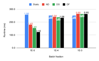
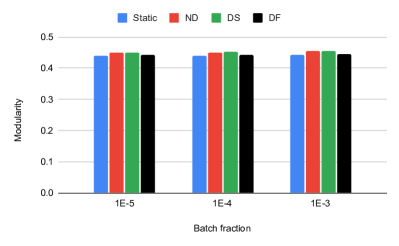
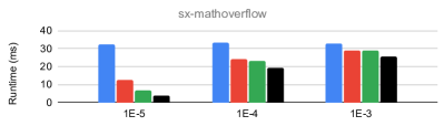
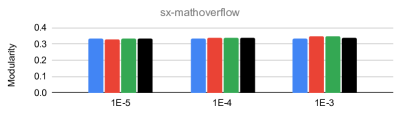
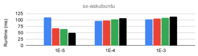
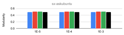
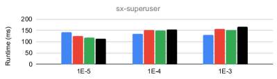
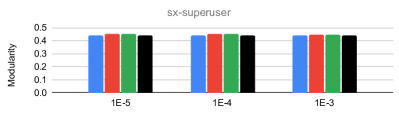
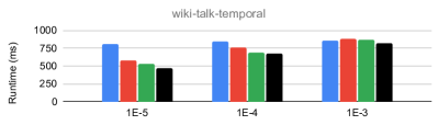
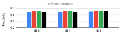
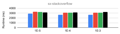
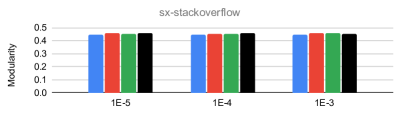
We also assess the performance of parallel implementations of Static, along with our improved ND, DS, and DF Leiden, on the real-world dynamic graphs listed in Table 2. These evaluations are conducted on batch updates of size to . For each batch size, as outlined in Section 5.1.4, we load of the graph, add reverse edges to ensure undirected edges, and then load edges (where is the batch size) across consecutive batch updates. Figure 13(a) illustrates the overall runtime for each method across all graphs and batch sizes, while Figure 13(b) shows the overall modularity of the resulting communities. Additionally, Figures 13(c) and 13(d) display the average runtime and modularity achieved by each method for the individual dynamic graphs in the dataset.
Figure 13(a) shows that, on average, ND, DS, and DF Leiden are , , and faster than Static Leiden for batch updates of size to . We now discuss why these methods provide only modest speed improvements over Static Leiden. Our experiments reveal that only around of the total runtime for ND, DS, and DF Leiden is spent in the first pass of the algorithm. Additionally, for large batch updates, a significant portion of the runtime is dedicated to the splitting, refinement, and aggregation phases. For smaller batch updates, a substantial amount of time is spent renumbering communities. As a result, the overall speedup of ND, DS, and DF Leiden compared to Static Leiden remains limited.