A Global Coordinate-Free Approach to Invariant Contraction on Homogeneous Manifolds

Abstract

In this work, we provide a global condition for contraction with respect to an invariant Riemannian metric on reductive homogeneous spaces. Using left-invariant frames, vector fields on the manifold are horizontally lifted to the ambient Lie group, where the Levi-Civita connection is globally characterized as a real matrix multiplication. By linearizing in these left-invariant frames, we characterize contraction using matrix measures on real square matrices, avoiding the use of local charts. Applying this global condition, we provide a necessary condition for a prescribed subset of the manifold to possibly admit a contracting system with respect to an invariant metric. Applied to the sphere, this condition implies that no closed hemisphere can be contained in a contraction region. Finally, we apply our results to compute reachable sets for an attitude control problem.

I INTRODUCTION

Contraction theory provides a powerful suite of tools for analyzing nonlinear systems by analyzing the distance between pairs of trajectories; see [1, 2, 3] for recent surveys on the rich history of contraction analysis in dynamical systems. Contraction is usually studied on vector spaces, from two main perspectives: i) after equipping the state space with a Riemannian structure, the (generalized) Demidovich conditions [4] verify stability of the variational system [5, 6]; ii) equipping the state space with a norm, the matrix measure of the linearization verifies contraction [7, 8]. Some applications of contraction analysis include: analysis and design of networked systems [9, 10]; control design on Lie groups using control contraction metrics [6, 11]; Lyapunov function design for monotone systems [12]; and robustness analysis of implicit neural networks [13].

There are some approaches formulating contraction in the coordinate-free setting of differentiable manifolds. One approach uses tools from affine differential geometry [14], where contraction on Riemannian manifolds is characterized using the Levi-Civita connection associated to the metric. Another approach uses a globally defined Finsler-Lyapunov function [15], where contraction on Finsler manifolds is characterized using Lyapunov conditions on the variational system. Recently, these results have been extended fully into the coordinate-free setting, where the contraction criterion was characterized using the complete lift of the system and a Finsler-Lyapunov function [16, 17]. In doing so, a converse result showed that every contractive system admits a Finsler-Lyapunov function. In this work, we simplify the contraction condition in the case where the metric is invariant under a group action. While this is a more restrictive setting, we are able to prove strong statements regarding the existence of contractive systems.

A manifold equipped with a transitive Lie group action is called a homogeneous space, and provides a canonical equivalence between points. When the relevant structures (e.g., metrics and connections) remain invariant under this equivalence, problems can often be simplified by lifting to the Lie group, providing a separate suite of group theoretic tools for global analysis which can improve theoretical [18, 19] and computational [20] capabilities. In control theory, homogeneous spaces have been studied in the framework of differential positivity [21], which is the generalization of monotonicity to manifolds [22]. In these settings, a cone field respecting the group action on the manifold improves tractability in verifying stable attractors for differentially positive systems [23].

Contributions  The main contribution of this work is an equivalent global condition for contraction with respect to an invariant metric on reductive homogeneous spaces, which we use to prove a necessary condition for the existence of a contracting system. We first recall existing results of how vector fields on the manifold can be expressed uniquely through their horizontal lift onto a horizontal bundle of a Lie group. In Lemma 1, using a left-invariant frame for the horizontal bundle, we linearize the dynamics into a real $m\times m$ matrix at each point along the actual manifold itself, allowing us to compute the Levi-Civita connection with a standard matrix multiplication. In Lemma 2, we show how the abstract contraction condition from [14] can be transformed into a familiar matrix measure computation. In Theorem 1, we use these facts to provide a global characterization of a contracting system with respect to an invariant metric.

Using this global definition, we provide a necessary condition for the existence of an invariant contracting system given a desired contraction region, which accounts for the underlying geometry of the space. Specifically, Theorem 2 shows how any invariant contraction region cannot contain the image of circular one-parameter subgroups acting on the manifold. In particular, Corollary 2 elaborates how this implies that a contraction region cannot contain any closed geodesics if the underlying space is naturally reductive (e.g., Riemannian symmetric). As an example, we show how the sphere cannot contract with respect to an invariant metric on any region containing a closed hemisphere. Finally, we use invariant contraction theory to prove nonexpansion of an attitude control system on $SO(3)$, allowing us to simplify reachable set computation.

II BACKGROUND AND NOTATION

Let $M$ denote a ($C^{\infty}$ smooth) manifold, let $T_{p}M$ denote the tangent space at $p\in M$, and $TM=\bigsqcup_{p\in M}T_{p}M$ denote the tangent bundle. Given a smooth map $f:M\to N$ between manifolds $M$ and $N$, let $Tf:TM\to TN$ denote the tangent (differential) map, and $T_{p}f:T_{p}M\to T_{f(p)}N$ denote its restriction to $T_{p}M$.

A vector field $X$ on $M$ (denoted $X\in\Gamma^{\infty}(TM)$) is a smooth section of the tangent bundle, i.e., $X(p)\in T_{p}M$ for every $p\in M$. Given $X\in\Gamma^{\infty}(TM)$, an integral curve at $p\in M$ is a curve $\gamma:J_{p}\to M$ satisfying $\gamma(0)=p$ and $\gamma^{\prime}(t)=X(\gamma(t))$ for every $t\in J_{p}$. $\gamma$ is called maximal if it is a well defined integral curve over the largest possible interval $J_{p}$ containing $0$. The flow of $X$ is the unique map $\Phi_{X}:J\times V\to M$, $(t,p)\mapsto\Phi_{X}^{t}(p)$, where $V$ is an open neighborhood of $p\in M$, and $t\mapsto\Phi_{X}^{t}(p)$ is the maximal integral curve of $X$ through $p$. Given a subset $U\subseteq M$, $X$ is called forward complete on $U$ if $\sup J_{p}=+\infty$ for every $p\in U$.

For a smooth map $f:M\to\mathbb{R}$ and $X\in\Gamma^{\infty}(TM)$, let $\mathcal{L}_{X}f$ denote the Lie derivative, where for $p\in M$, $\mathcal{L}_{X}f(p)=\lim_{h\to 0}\frac{f(\Phi_{X}^{t}(p))-f(p)}{h}$. An affine connection $\nabla:\Gamma^{\infty}(TM)\times\Gamma^{\infty}(TM)\to\Gamma^{\infty}(TM)$ on $M$ is a bilinear map where for every smooth $f:M\to\mathbb{R}$ and $X,Y\in\Gamma^{\infty}(TM)$, (i) $\nabla_{fX}Y=f\nabla_{X}Y$, and (ii) $\nabla_{X}(fY)=(\mathcal{L}_{X}f)Y+f\nabla_{X}Y$. A Riemannian metric $\langle\langle\cdot,\cdot\rangle\rangle$ is a $(0,2)$-tensor field on $M$ such that $\langle\langle\cdot,\cdot\rangle\rangle_{p}:T_{p}M\times T_{p}M\to\mathbb{R}$ is an inner product in the tangent space $T_{p}M$ for every $p\in M$. The Riemannian manifold $(M,\langle\langle\cdot,\cdot\rangle\rangle)$ is endowed with a unique metric-preserving torsion-free affine connection called the Levi-Civita connection. For a curve $\gamma:J\to M$, let $\ell(\gamma)=\int_{J}\sqrt{\langle\langle\gamma^{\prime}(t),\gamma^{\prime}(t)\rangle\rangle_{\gamma(t)}}dt$ be its length. $M$ is a metric space with the Riemannian distance $d$, where for $x,y\in M$, $d(x,y)=\inf\{\ell(\gamma):\gamma:[0,1]\to M,\gamma(0)=x,\gamma(1)=y\}$. A subset $U\subseteq M$ is $K$-reachable for $K\geq 1$ if for every $x,y\in U$, there exists a curve $\gamma:[0,1]\to U$, $\gamma(0)=x$, $\gamma(1)=y$ satisfying $\ell(\gamma)\leq Kd(x,y)$.

A Lie group $G$ is a manifold with compatible group structure, i.e., the group operation is a smooth map from the product manifold $G\times G$ to $G$, and the group inverse is a smooth map from $G$ to $G$. Let $\ell_{g}:G\to G$, $h\mapsto\ell_{g}(h)=gh$ for every $g\in G$ denote the left translation map. Let $\mathfrak{g}=T_{e}G$ denote the Lie algebra, and for $X\in\mathfrak{g}$, let $X^{L}\in\Gamma^{\infty}(TG)$ denote the corresponding left-invariant vector field on $G$, i.e., $g\mapsto X^{L}(g)=T_{e}\ell_{g}(X)$. The space $\mathfrak{g}$ is endowed with the Lie bracket $[\cdot,\cdot]_{\mathfrak{g}}$ from the usual Lie bracket of vector fields, as $[X,Y]_{\mathfrak{g}}^{L}=[X^{L},Y^{L}]$. Let $\exp:\mathfrak{g}\to G$ denote the exponential map, i.e., $\exp(X)=\gamma(1)$ where $\gamma$ is the maximal integral curve of $X^{L}$ passing through $\gamma(0)=e$. Given $g\in G$, let $\operatorname{conj}_{g}:G\to G$, $g^{\prime}\mapsto\operatorname{conj}_{g}(g^{\prime})=gg^{\prime}g^{-1}$ denote conjugation by $g$, and let $\operatorname{Ad}_{g}:\mathfrak{g}\to\mathfrak{g}$, $X\mapsto\operatorname{Ad}_{g}(X)=T_{e}\operatorname{conj}_{g}(X)$ denote the adjoint representation.

We use Einstein’s summation convention, where repeated indices in a term are summed over, e.g., $a^{i}x_{i}=\sum_{i=1}^{n}a^{i}x_{i}$. Let $\delta_{ij}$ denote the Kronecker delta function, where $\delta_{ij}=0$ for every $i\neq j$ and $\delta_{ij}=1$ when $i=j$.

III REDUCTIVE HOMOGENEOUS SPACES AND INVARIANT RIEMANNIAN METRICS

In this section, we summarize several key facts about reductive homogeneous spaces. We refer to the following modern sources: [19, Section 23] for an in depth discussion on reductive homogeneous spaces, and [24] regarding invariant metrics and affine connections on homogeneous spaces through the lens of horizontal lifts. We also refer to the original work [18] characterizing invariant affine connections.

III-A Homogeneous spaces

Let $G$ be a connected Lie group and $M$ be a manifold. A transitive (left) action of $G$ on $M$ is a smooth map $\lambda:G\times M\to M$ satisfying the following axioms:

1. $\lambda(e,p)=p$ for every $p\in M$;

2. $\lambda(g,\lambda(g^{\prime},p))=\lambda(gg^{\prime},p)$ for every $g,g^{\prime}\in G$, $p\in M$;

3. For every $p,q\in M$, there exists $g\in G$ such that $\lambda(g,p)=q$ (transitivity).

$(M,\lambda)$ is called a homogeneous space. Fix a point $o\in M$, and let $G_{o}=\{g\in G:\lambda(g,o)=o\}$ denote its stabilizer, which forms a closed subgroup of $G$. One can equivalently construct the homogeneous space $M$ by taking the quotient $G/G_{o}$, with the following equivalence between (left) cosets and points in $M$, $gG_{o}\iff\lambda(g,o)$. In fact, given any closed subgroup $H\subseteq G$, the quotient $G/H$ is a homogeneous space under the natural action $\lambda(g^{\prime},gH)=(g^{\prime}g)H$. Thus, we use the notation $M=G/H$ to denote a homogeneous space with action $\lambda$, and consider points $p\in M$ the same as a point $gH$ given a representative $g$ in the corresponding coset. For $g\in G$, let $\lambda_{g}:M\to M$, $\lambda_{g}(p)=\lambda(g,p)$ denote the associated diffeomorphism. Let $\pi:G\to G/H$, $g\mapsto\pi(g)=gH$ denote the canonical projection.

III-B Horizontal lifts

An important class of homogeneous spaces arises when the Lie algebra $\mathfrak{g}$ can be decomposed into the direct sum of two subspaces with some additional structure.

Definition 1 (Reductive homogeneous space).

Let $G$ be a Lie group with Lie algebra $\mathfrak{g}$ and $H\subseteq G$ denote a closed subgroup with Lie subalgebra $\mathfrak{h}\subseteq\mathfrak{g}$. The homogeneous space $G/H$ is called reductive if there exists a subspace $\mathfrak{m}\subseteq\mathfrak{g}$ such that $\mathfrak{g}=\mathfrak{h}\oplus\mathfrak{m}$, and $\operatorname{Ad}_{h}(\mathfrak{m})\subseteq\mathfrak{m}$ for every $h\in H$ ($\mathfrak{m}$ is $\operatorname{Ad}_{H}$-invariant).

For a reductive homogeneous space $G/H$ with reductive decomposition $\mathfrak{g}=\mathfrak{h}\oplus\mathfrak{m}$, define the horizontal bundle $\operatorname{Hor}(G)=\bigsqcup_{g\in G}\operatorname{Hor}(G)_{g}$, where the fiber $\operatorname{Hor}(G)_{g}=T_{e}\ell_{g}(\mathfrak{m})$. Given a vector field $X\in\Gamma^{\infty}(TM)$, define the horizontal lift $\overline{X}\in\Gamma^{\infty}(\operatorname{Hor}(G))$ as the unique vector field where for every $g\in G$,

$$\overline{X}(g)=(T_{g}\pi\big{|}_{\operatorname{Hor(G)}_{g}})^{-1}X(\pi(g)),$$

where $T_{g}\pi\big{|}_{\operatorname{Hor(G)}_{g}}:\operatorname{Hor}(G)_{g}\to T_{gH}M$ is the invertible restriction of $T_{g}\pi$. The horizontal lift takes the vector field $X$ on $G/H$ and defines a vector field $\overline{X}$ on $G$, where $\overline{X}(g)$ lives on the subspace $T_{e}\ell_{g}(\mathfrak{m})=\operatorname{Hor}(G)_{g}$, and the projection $T_{g}\pi(\overline{X}(g))$ is equivalent for any representative $g$ in $gH$.

III-C Invariant structures on homogeneous spaces

In this section, we discuss various invariant geometric structures on homogeneous spaces. Throughout this section, let $M=G/H$ denote a reductive homogeneous space with reductive decomposition $\mathfrak{g}=\mathfrak{h}\oplus\mathfrak{m}$.

Metrics A Riemannian metric $\langle\langle\cdot,\cdot\rangle\rangle$ on $M$ is invariant if for every $g\in G$, $p\in M$, and $v_{p},w_{p}\in T_{p}M$,

$$\langle\langle v_{p},w_{p}\rangle\rangle_{p}=\langle\langle T_{p}\lambda_{g}(v_{p}),T_{p}\lambda_{g}(w_{p})\rangle\rangle_{\lambda_{g}(p)}.$$

An inner product $\langle\cdot,\cdot\rangle_{\mathfrak{m}}:\mathfrak{m}\times\mathfrak{m}\to\mathbb{R}$ is $\operatorname{Ad}_{H}$-invariant if for every $h\in H$ and $X,Y\in\mathfrak{m}$,

$$\langle\operatorname{Ad}_{h}(X),\operatorname{Ad}_{h}(Y)\rangle=\langle X,Y\rangle,$$

It is known [19, Prop. 23.22] that there is a one-to-one correspondence between $\operatorname{Ad}_{H}$-invariant inner products on $\mathfrak{m}$ and invariant Riemannian metrics on $M$ by requiring the map $T_{e}\pi|_{\mathfrak{m}}:\mathfrak{m}\to T_{eH}M$ to be an isometry.

Given an inner product $\langle\cdot,\cdot\rangle_{\mathfrak{m}}$ and a basis $\mathcal{A}=\{A_{1},\dots,A_{m}\}$ for $\mathfrak{m}$, we define the inner product $\langle\cdot,\cdot\rangle_{\mathcal{A}}$ on $\mathbb{R}^{m}$, such that $\langle v,w\rangle_{\mathcal{A}}=\langle v^{i}A_{i},w^{j}A_{j}\rangle_{\mathfrak{m}}$.

Connections An affine connection $\nabla$ on $M$ is invariant if for every $g\in G$ and $X,Y\in\Gamma^{\infty}(TM)$,

$$\nabla_{X}Y=(\lambda_{g^{-1}})_{*}(\nabla_{(\lambda_{g})_{*}X}(\lambda_{g})_{*}Y),$$

where $(\lambda_{g})_{*}=T\lambda_{g}\circ X\circ\lambda_{g^{-1}}$ denotes the pushforward. It was originally shown by Nomizu [18, Thm. 8.1] that there is a one-to-one correspondence between bilinear maps $\alpha:\mathfrak{m}\times\mathfrak{m}\to\mathfrak{m}$ and invariant affine connections $\nabla$ on $M$. We follow the treatment from [24, Thm. 4.15, Def. 4.16], where given bilinear $\alpha:\mathfrak{m}\times\mathfrak{m}\to\mathfrak{m}$, the unique invariant covariant derivative $\nabla^{\alpha}$ is defined by

$$\nabla^{\alpha}_{X_{M}}Y_{M}(eH)=T_{e}\pi(-[X,Y]_{\mathfrak{m}}+\alpha(X,Y)),$$

for every $X,Y\in\mathfrak{m}$, where $[X,Y]_{\mathfrak{m}}$ is the component of $[X,Y]_{\mathfrak{g}}$ on $\mathfrak{m}$ (this is not necessarily a Lie bracket on $\mathfrak{m}$), and $X_{M}$ is the fundamental vector field

$$X_{M}(gH)=\frac{d}{dt}\Big{|}_{t=0}\lambda(\exp(tX),gH).$$

Let $\mathcal{A}=\{A_{1},\dots,A_{m}\}\subseteq\mathfrak{m}$ be a basis, $X,Y\in\Gamma^{\infty}(TM)$, and $\overline{X},\overline{Y}\in\Gamma^{\infty}(\operatorname{Hor}(G))$ be their horizontal lifts. Since $\{A_{1}^{L}(g),\dots,A_{m}^{L}(g)\}$ span $\operatorname{Hor}(G)_{g}$ for every $g$, one can express the horizontal lift as the linear combinations $\overline{X}=\overline{X}^{i}A_{i}^{L}$ and $\overline{Y}=\overline{Y}^{i}A_{i}^{L}$, for curves $\overline{X}^{i}:G\to\mathbb{R}$ and $\overline{Y}^{i}:G\to\mathbb{R}$ for every $i=1,\dots,m$. As shown in [24, Thm 4.15], the covariant derivative $\nabla^{\alpha}_{X}Y$ between any two vector fields can be expressed through these horizontal lifts as

$$\overline{\nabla^{\alpha}_{X}Y}=(\mathcal{L}_{\overline{X}}Y^{j})A_{j}^{L}+X^{j}Y^{k}\alpha_{jk}^{L},$$

where $\alpha_{jk}=\alpha^{i}_{jk}A_{i}=\alpha(A_{j},A_{k})\in\mathfrak{m}$ for each $j,k\in\{1,\dots,m\}$, with $\alpha^{i}_{jk}\in\mathbb{R}$.

Levi-Civita It was originally shown in [18, Thm. 13.1] that the Levi-Civita connection $\nabla^{\mathrm{LC}}$ associated to an invariant metric $\langle\langle\cdot,\cdot\rangle\rangle$ induced by $\operatorname{Ad}_{H}$-invariant inner product $\langle\cdot,\cdot\rangle_{\mathfrak{m}}$ is indeed an invariant connection, and characterized by the bilinear map

$$\alpha(X,Y)=\tfrac{1}{2}[X,Y]_{\mathfrak{m}}+U(X,Y),$$ (1)

where $U(X,Y)$ is uniquely determined by

$$\langle U(X,Y),Z\rangle=\tfrac{1}{2}(\langle[X,Z]_{\mathfrak{m}},Y\rangle+\langle X,[Y,Z]_{\mathfrak{m}}\rangle).$$ (2)

Uniqueness follows by non-degeneracy of $\langle\cdot,\cdot\rangle_{\mathfrak{m}}$.

In two special cases, the expression for $\alpha$ for the invariant Levi-Civita connection is simplified.

Definition 2.

Let $G/H$ be a homogeneous space with invariant Riemannian metric $\langle\langle\cdot,\cdot\rangle\rangle$ induced by $\operatorname{Ad}_{H}$-invariant inner product $\langle\cdot,\cdot\rangle_{\mathfrak{m}}$. $G/H$ is called naturally reductive if for every $X,Y,Z\in\mathfrak{m}$,

$$\langle[X,Z]_{\mathfrak{m}},Y\rangle+\langle X,[Y,Z]_{\mathfrak{m}}\rangle=0.$$

In the case of a naturally reductive homogeneous space, $U(X,Y)=0$, so $\alpha(X,Y)=\frac{1}{2}[X,Y]_{\mathfrak{m}}$ recovers the Levi-Civita connection. When $G/H$ is naturally reductive, the geodesics coincide with curves of the form $\pi(g\exp(tX))$, $X\in M$ [19, Prop. 23.28].

Definition 3.

Let $G$ be a connected Lie group, and $\sigma:G\to G$ be a smooth involutive automorphism, i.e., $\sigma^{2}=\operatorname{id}$. Let $H_{\sigma}$ denote the set of fixed points of $\sigma$, which is a closed subgroup of $G$, and let $(H_{\sigma})_{0}$ denote the component containing $e\in G$. A homogeneous space $G/H$ is called a symmetric homogeneous space if $(H_{\sigma})_{0}\subseteq H\subseteq H_{\sigma}$.

For a symmetric homogeneous space $(G/H,\sigma)$ with invariant metric $\langle\langle\cdot,\cdot\rangle\rangle$, it is known that $[\mathfrak{m},\mathfrak{m}]_{\mathfrak{g}}\subseteq\mathfrak{h}$, so $[\mathfrak{m},\mathfrak{m}]_{\mathfrak{m}}=0$ [18, Sec. 14]. As a corollary, the choice $\alpha=0$ recovers the Levi-Civita connection $\nabla^{\mathrm{LC}}=\nabla^{\alpha}$.

III-D Examples of reductive Riemannian homogeneous spaces

Figure 1: A visualization of the reductive homogeneous space $\mathbb{S}^{2}=SO(3)/SO(2)$. Left: An element $R\in SO(3)$ acts on $o$, resulting in the vector $p=Ro$. Right: The stabilizer $H=SO(2)$ is the set of rotations $R$ which fix $o$ ($Ro=o$). The element $X\in\mathfrak{m}$, a $\operatorname{Ad}_{H}$-invariant subspace, generates the green curve $\pi(\exp(tX))$ and arrives to $p=\pi(\exp(X))$.

In the sequel, we will consider the following structure.

Definition 4.

Let $M=G/H$ be a reductive homogenous space, with reductive decompostion $\mathfrak{g}=\mathfrak{h}\oplus\mathfrak{m}$, $\operatorname{Ad}_{H}$-invariant inner product $\langle\cdot,\cdot\rangle_{\mathfrak{m}}$. We call the tuple $(G,H,\langle\cdot,\cdot\rangle_{\mathfrak{m}})$ a reductive Riemannian homogeneous space.

We briefly present several examples of reductive Riemannian homogeneous spaces.

1. $(V,W^{\perp},\langle\cdot,\cdot\rangle|_{W\times W})$—a linear subspace $W\subseteq V$ of inner product space $(V,\langle\cdot,\cdot\rangle)$, as $W=V/W^{\perp}$, where $W^{\perp}$ is the orthogonal complement of $W$.

2. $(G,\{e\},\langle\langle\cdot,\cdot\rangle\rangle)$—a Lie group $G$ with a left-invariant metric. $G$ acts on itself on the left as $\lambda(g_{1},g_{2})=g_{1}g_{2}$. The metric is left-invariant if $\langle\langle T_{e}\ell_{g}(X),T_{e}\ell_{g}(Y)\rangle\rangle_{g}=\langle\langle X,Y\rangle\rangle_{e}$. Here $H$ is trivial, so $\mathfrak{m}=\mathfrak{g}$ and $\langle\langle\cdot,\cdot\rangle\rangle_{e}$ is automatically $\operatorname{Ad}_{H}$-invariant.

3. $(G,\{e\},\langle\langle\cdot,\cdot\rangle\rangle)$—a Lie group $G$ with a bi-invariant metric is a naturally reductive space. The metric is bi-invariant if $\langle\langle T_{e}r_{g}(X),T_{e}r_{g}(Y)\rangle\rangle_{g}=\langle\langle T_{e}\ell_{g}(X),T_{e}\ell_{g}(Y)\rangle\rangle_{g}=\langle\langle X,Y\rangle\rangle_{e}$.

4. $(SO(n+1),SO(n),\langle\langle\cdot,\cdot\rangle\rangle)$—The $n$-dimensional sphere $\mathbb{S}^{n}$ is diffeomorphic to the quotient $SO(n+1)/SO(n)$. To see this for $\mathbb{S}^{2}$, consider the action of $G=SO(3)$ on vectors of $\mathbb{R}^{3}$ as rotations (matrix multiplication). Taking $o=[1\ 0\ 0]^{T}$, the orbit $G\cdot o$ sweeps out the entire unit sphere in $\mathbb{R}^{3}$, i.e., $\mathbb{S}^{2}$. The stabilizer $G_{o}$ is the set of rotations about $o$, namely of the form $\begin{bmatrix}\cos(\theta)&-\sin(\theta)&0\\ \sin(\theta)&\cos(\theta)&0\\ 0&0&1\end{bmatrix}$, which is diffeomorphic to $SO(2)$. Taking the metric $\langle X,Y\rangle_{\mathfrak{g}}=\operatorname{trace}(X^{T}Y)$, it is easy to show that the restriction $\langle\cdot,\cdot\rangle_{\mathfrak{m}}=\tfrac{1}{2}\langle\cdot,\cdot\rangle_{\mathfrak{g}}|_{\mathfrak{m}\times\mathfrak{m}}$ is $\operatorname{Ad}_{G_{o}}$-invariant, giving rise to an invariant metric $\langle\langle\cdot,\cdot\rangle\rangle$ on $\mathbb{S}^{2}=SO(3)/SO(2)$ (matching the standard round metric). This is visualized in Figure 1.

IV INVARIANT CONTRACTION THEORY

In [14], contraction with respect to a distance defined by a Riemannian metric was formulated in a coordinate-free manner using the Levi-Civita connection.

Definition 5 (Contracting system [14, Def. 2.1]).

Let $M$ be a manifold, $X\in\Gamma^{\infty}(TM)$, and $U\subseteq M$ be a connected set. Let $\langle\langle\cdot,\cdot\rangle\rangle$ be a Riemannian metric on $M$. We say that $(U,X,\langle\langle\cdot,\cdot\rangle\rangle,c)$ is a contracting system on $M$ at rate $c<0$ if for every $x\in U$ and $v\in T_{x}M$,

$$\langle\langle\nabla_{v}X,v\rangle\rangle_{x}\leq c\langle\langle v,v\rangle\rangle_{x},$$

where $\nabla$ denotes the Levi-Civita connection of $\langle\langle\cdot,\cdot\rangle\rangle$.

Checking this condition in practice, however, requires the use of local charts to verify the generalized Demidovich conditions [14, Prop. 2.4]. In this section, for reductive homogeneous spaces equipped with an invariant metric, we develop a global characterization of a contracting system, using matrix measures on real $m\times m$ dimensional matrices.

IV-A Linearization in left-invariant frames

Given a vector field $X\in\Gamma^{\infty}(TM)$, we first consider the linearization of the horizontal lift $\overline{X}\in\operatorname{Hor}(G)$, with respect to a left-invariant frame from a basis of $\mathfrak{m}$.

Definition 6 (Horizontal linearization in left-invariant frame).

Let $(G,H,\langle\cdot,\cdot\rangle_{\mathfrak{m}})$ be a reductive Riemannian homogeneous space, and let $\mathcal{A}=\{A_{1},\dots,A_{m}\}$ be a orthonormal basis for $\mathfrak{m}$. For a vector field $\overline{X}\in\Gamma^{\infty}(\operatorname{Hor}(G))$, characterized by $\overline{X}=\overline{X}^{i}A^{L}_{i}$ for curves $\overline{X}^{i}:G\to\mathbb{R}$, define the map $\partial_{\mathcal{A}}\overline{X}:G\to\mathbb{R}^{m\times m}$,

$$(\partial_{\mathcal{A}}\overline{X})^{i}_{j}=\mathcal{L}_{A_{j}^{L}}\overline{X}^{i}+\overline{X}^{k}\alpha^{i}_{jk},$$

with $\alpha^{i}_{jk}$ defined as $\alpha(A_{j},A_{k})=\alpha^{i}_{jk}A_{i}$ for the bilinear map $\alpha:\mathfrak{m}\times\mathfrak{m}\to\mathfrak{m}$ from (1).

Lemma 1 (Properties of $\partial_{\mathcal{A}}\overline{X}$).

Let $(G,H,\langle\cdot,\cdot\rangle_{\mathfrak{m}})$ be a reductive Riemannian homogeneous space and $\mathcal{A}$ be an orthonormal basis for $\mathfrak{m}$. Let $X\in\Gamma^{\infty}(TM)$ and $\overline{X}\in\Gamma^{\infty}(\operatorname{Hor}(G))$ be its horizontal lift. The following statements hold:

1. For any $v\in\mathbb{R}^{m}$, and $V\in\Gamma^{\infty}(TM)$ defined by $V(gH)=T_{g}\pi(v^{j}A_{j}^{L}(g))$,

   $$\overline{\nabla_{V}X}=(\partial_{\mathcal{A}}\overline{X})^{i}_{j}v^{j}A_{i}^{L}=((\partial_{\mathcal{A}}\overline{X})v)^{\wedge L},$$

   where $\wedge:\mathbb{R}^{n}\to\mathfrak{g}$ is the basis expansion.

2. For any $g_{1},g_{2}$ such that $g_{1}H=g_{2}H$,

   $$\partial_{\mathcal{A}}\overline{X}(g_{1})=\partial_{\mathcal{A}}\overline{X}(g_{2}).$$

Proof.

Let $v\in\mathbb{R}^{m}$, $g\in G$. Let $\overline{X}^{j}A_{j}^{L}=\overline{X}$ for $\overline{X}^{j}:G\to\mathbb{R}$, $j=1,\dots,m$. Regarding (i), since $\overline{V}=v^{j}A_{j}^{L}$,

$$\overline{\nabla_{V}X} =(\mathcal{L}_{v^{j}A_{j}^{L}}X^{i})A_{i}^{L}+v^{j}X^{k}\alpha_{jk}^{L}$$

$$=v^{j}(\mathcal{L}_{A_{j}^{L}}\overline{X}^{i})A_{i}^{L}+v^{j}X^{k}\alpha_{jk}^{i}A_{i}^{L}$$

$$=(\mathcal{L}_{A_{j}^{L}}\overline{X}^{i}+\overline{X}^{k}\alpha_{jk}^{i})v^{j}A_{i}^{L}=(\partial\overline{X})_{j}^{i}v^{j}A_{i}^{L}.$$

Regarding (ii), let $g_{1}H=g_{2}H$. Since $T_{g_{1}}\pi(\overline{\nabla_{v^{j}A_{j}^{L}}X}(g_{1}))=T_{g_{2}}\pi(\overline{\nabla_{v^{j}A_{j}^{L}}X}(g_{2}))$,

$$T_{g_{1}}\pi((\partial_{\mathcal{A}}\overline{X}(g_{1}))_{j}^{i}v^{j}A_{i}^{L}(g_{1}))=T_{g_{2}}\pi((\partial_{\mathcal{A}}\overline{X}(g_{2}))_{j}^{i}v^{j}A_{i}^{L}(g_{2})),$$

which implies by linearity of $T_{g}\pi$ that

$$(\partial_{\mathcal{A}}\overline{X}(g_{1}))_{j}^{i}v^{j}T_{g_{1}}\pi(A_{i}^{L}(g_{1}))=(\partial_{\mathcal{A}}\overline{X}(g_{2}))_{j}^{i}v^{j}T_{g_{2}}\pi(A_{i}^{L}(g_{2})).$$

Finally, since $T_{g_{1}}\pi(A_{i}^{L}(g_{1}))=T_{g_{2}}\pi(A_{i}^{L}(g_{2}))$ by definition of the horizontal lift, we have $(\partial_{\mathcal{A}}\overline{X}(g_{1}))_{j}^{i}v^{j}=(\partial_{\mathcal{A}}\overline{X}(g_{2}))_{j}^{i}v^{j}$. Since $v$ was arbitrary, $\partial_{\mathcal{A}}\overline{X}(g_{1})=\partial_{\mathcal{A}}\overline{X}(g_{2})$. ∎

Lemma 1 highlights two key important facts about Definition 6: (i) shows how the invariant affine connection can be computed using a real matrix multiplication; (ii) shows that the matrix coincides on every coset in the space $G/H$.

Definition 7 (Linearization on homogeneous space).

Let $(G,H,\langle\cdot,\cdot\rangle_{\mathfrak{m}})$ be a reductive Riemannian homogeneous space, and let $\mathcal{A}$ be an orthonormal basis for $\mathfrak{m}$. For a vector field $X\in\Gamma^{\infty}(T(G/H))$ with horizontal lift $\overline{X}\in\Gamma^{\infty}(\operatorname{Hor}(G))$, define the map $\partial_{\mathcal{A}}X:G/H\to\mathbb{R}^{m\times m}$,

$$\partial_{\mathcal{A}}X(gH)=\partial_{\mathcal{A}}\overline{X}(g).$$

By Part (ii) of Lemma 1, $\partial_{\mathcal{A}}X$ is well defined since $\partial_{\mathcal{A}}\overline{X}$ coincides on every coset.

Lemma 2.

Let $(G,H,\langle\cdot,\cdot\rangle_{\mathfrak{m}})$ be a reductive Riemannian homogeneous space, and let $\mathcal{A}$ be an orthonormal basis for $\mathfrak{m}$. Let $X\in\Gamma^{\infty}(TM)$ and $\overline{X}\in\Gamma^{\infty}(\operatorname{Hor}(G))$ be its horizontal lift. Let $\langle\langle\cdot,\cdot\rangle\rangle$ be the invariant Riemannian metric on $M=G/H$ induced by $\langle\cdot,\cdot\rangle_{\mathfrak{m}}$, and let $\nabla$ denote the corresponding Levi-Civita connection. For any $g\in G$, $v\in\mathbb{R}^{m}$, and $V\in\Gamma^{\infty}(TM)$ such that $V(gH)=T_{g}\pi(v^{j}A_{j}^{L}(g))$,

$$\langle\langle\nabla_{V}X,V\rangle\rangle_{gH} =\langle\partial_{\mathcal{A}}X(g)^{i}_{j}v^{j}A_{i},v^{i}A_{i}\rangle_{\mathfrak{m}}$$

$$=\langle\partial_{\mathcal{A}}X(g)v,v\rangle_{\mathcal{A}}.$$

Proof.

Let $g\in G$ and $v\in\mathbb{R}^{m}$. For notational brevity, let $\partial\overline{X}:=\partial_{\mathcal{A}}\overline{X}(g)$. Applying Part (i) of Lemma 1,

$$\langle\langle\nabla_{V}X,V\rangle\rangle_{gH} =\langle\langle T_{g}\pi((\partial\overline{X})^{i}_{j}v^{j}A_{i}^{L}),T_{g}\pi(v^{i}A_{i}^{L})\rangle\rangle_{gH}.$$

By invariance of the metric $\langle\langle\cdot,\cdot\rangle\rangle$,

$$\langle\langle\nabla_{V}X,V\rangle\rangle_{gH} =\langle\langle T_{gH}\lambda_{g^{-1}}(T_{g}\pi((\partial\overline{X})^{i}_{j}v^{j}A_{i}^{L})),$$

$$\quad\quad T_{gH}\lambda_{g^{-1}}(T_{g}\pi(v^{i}A_{i}^{L}))\rangle\rangle_{eH}.$$

Using the chain rule, $T_{gH}\lambda_{g^{-1}}\circ T_{g}\pi=T_{g}(\lambda_{g^{-1}}\circ\pi)$, and $\lambda(g^{-1},\pi(\cdot))=\lambda(e,\pi(\ell_{g^{-1}}(\cdot)))=(\pi\circ\ell_{g^{-1}})(\cdot)$. Thus,

$$T_{gH} \lambda_{g^{-1}}(T_{g}\pi((\partial\overline{X})^{i}_{j}v^{j}A_{i}^{L}))=T_{e}\pi(T_{g}\ell_{g^{-1}}((\partial\overline{X})^{i}_{j}v^{j}A_{i}^{L}))$$

$$=(\partial\overline{X})^{i}_{j}v^{j}T_{e}\pi(T_{g}\ell_{g^{-1}}(A_{i}^{L}))=(\partial\overline{X})^{i}_{j}v^{j}T_{e}\pi(A_{i}^{L})$$

$$=(\partial\overline{X})^{i}_{j}v^{j}A_{i},$$

and similarly, $T_{gH}\lambda_{g^{-1}}(T_{g}\pi(v^{i}A_{i}^{L}))=v^{i}A_{i}$. ∎

Remark 1.

Since $\langle\langle\nabla_{V}X,V\rangle\rangle_{gH}$ does not depend on the choice of reductive orthonormal basis $\mathcal{A}$, an immediate corollary of Lemma 2 is that the quantity $\langle\partial_{\mathcal{A}}X(g)v,v\rangle_{\mathcal{A}}$ is independent of the choice of $\mathcal{A}$.

IV-B Invariant contracting systems

Using Lemma 2, we define the matrix measure of the linearization as the supremum over vectors of unit length in any orthonormal basis.

Definition 8 (Matrix measure).

Let $(G,H,\langle\cdot,\cdot\rangle_{\mathfrak{m}})$ be a reductive Riemannian homogeneous space. For a vector field $X\in\Gamma^{\infty}(T(G/H))$, define the map $\mu(\partial X(\cdot)):G/H\to\mathbb{R}$,

$$\mu(\partial X(p))=\sup_{v\in\mathbb{R}^{m},\langle v,v\rangle_{\mathcal{A}}=1}\langle\partial_{\mathcal{A}}X(p)v,v\rangle_{\mathcal{A}},$$

where $\mathcal{A}$ is any orthonormal basis for $\mathfrak{m}$. This is well defined by Remark 1.

Strictly speaking, $\mu(\partial X(\cdot))$ is notation for a single map, not the composition of $\mu$ and $\partial X$, since $\partial X$ is only defined with respect to a basis. We adopt this notation to connect to the traditional concept of a matrix measure. Once a basis $\mathcal{A}$ is chosen for $\mathfrak{m}$, this can be regarded as the composition, since $\partial_{\mathcal{A}}X(gH)$ is a real $m\times m$ matrix and $\mu$ is the usual matrix measure.

Definition 9 (Invariant contracting system).

Let $M=G/H$ be a reductive homogeneous space with reductive decomposition $\mathfrak{g}=\mathfrak{h}\oplus\mathfrak{m}$. Let $X\in\Gamma^{\infty}(TM)$, $U\subseteq M$ be connected, and $\langle\cdot,\cdot\rangle_{\mathfrak{m}}$ be an $\operatorname{Ad}_{H}$-invariant inner product on $\mathfrak{m}$. We say that $(U,X,\langle\cdot,\cdot\rangle_{\mathfrak{m}},c)$ is an invariant contracting system on $M$ at rate $c<0$ if for every $p\in U$,

$$\mu(\partial X(p))\leq c.$$

We now present the first Theorem of this work, which connects this condition to the original notion of a contracting system from Definition 5.

Theorem 1.

Let $M=G/H$ be a reductive homogeneous space with reductive decomposition $\mathfrak{g}=\mathfrak{h}\oplus\mathfrak{m}$. Let $X\in\Gamma^{\infty}(TM)$, $U\subseteq M$ be connected, $\langle\cdot,\cdot\rangle_{\mathfrak{m}}$ be an $\operatorname{Ad}_{H}$-invariant inner product on $\mathfrak{m}$, and $\langle\langle\cdot,\cdot\rangle\rangle$ be the associated invariant metric. The following are equivalent:

1. $(U,X,\langle\langle\cdot,\cdot\rangle\rangle,c)$ is a contracting system on $M$;

2. $(U,X,\langle\cdot,\cdot\rangle_{\mathfrak{m}},c)$ is an invariant contracting system on $M$.

Proof.

Let $\mathcal{A}=\{A_{1},\dots,A_{m}\}$ be an orthonormal basis for $\mathfrak{m}$. By Lemma 2, since any $V\in T_{p}M$ can be written as $T_{g}\pi(v^{j}A_{j}^{L}(g))$ given a representative $g\in G$ with $p=gH$,

$$\langle\langle\nabla_{V}X,V\rangle\rangle_{p}\leq c\langle\langle V,V\rangle\rangle_{p}\quad\forall p\in U,\,V\in T_{p}M$$

$$\iff\langle\partial_{\mathcal{A}}X(p)v,v\rangle_{\mathcal{A}}\leq c\langle v,v\rangle_{\mathcal{A}}\quad\forall p\in U,\,v\in\mathbb{R}^{m}$$

$$\iff\left\langle\partial_{\mathcal{A}}X(p)\tfrac{v}{|v|_{\mathcal{A}}},\tfrac{v}{|v|_{\mathcal{A}}}\right\rangle_{\mathcal{A}}\leq c\quad\forall p\in U,\,v\in\mathbb{R}^{m}\setminus\{0\}$$

$$\iff\left\langle\partial_{\mathcal{A}}X(p)w,w\right\rangle_{\mathcal{A}}\leq c\quad\forall p\in U,\,w\in\mathbb{R}^{m},|w|_{\mathcal{A}}=1,$$

completing the proof. ∎

As a consequence of Theorem 1, all of the desirable properties of a contracting system hold for an invariant contracting system [14, Prop. 2.5]. For instance, an important Corollary (the usual defining property of a contracting system) is that distances between any two trajectories initialized in the contraction region shrink exponentially at rate $c$.

Corollary 1 ([14, Theorem 2.3]).

Let $M=G/H$ be a reductive homogeneous space with reductive decomposition $\mathfrak{g}=\mathfrak{h}\oplus\mathfrak{m}$. If $(U,X,\langle\cdot,\cdot\rangle_{\mathfrak{m}},c)$ is an invariant contracting system on $M$, $U$ is a $K$-reachable forward $X$-invariant set, and $X$ is forward complete on $U$, for every $t\geq 0$,

$$d(\Phi_{X}^{t}(x_{0}),\Phi_{X}^{t}(y_{0}))\leq Ke^{ct}d(x_{0},y_{0}),$$

for any initial conditions $x_{0},y_{0}\in U$.

V A NECESSARY CONDITION FOR A CONTRACTIVE SYSTEM

As remarked in [14], a contracting system on a manifold $M$ satisfying the conditions of Corollary 1 necessarily implies that $U$ is a contractible subset, since a time reparameterization of the flow yields a homotopy of $U$ to the fixed equilibrium point. However, the converse is not generally true—given an arbitrary contractible subset $U$ of a manifold, there may not exist a vector field $X$ and a Riemannian metric $\langle\langle\cdot,\cdot\rangle\rangle$ such that $(U,X,\langle\langle\cdot,\cdot\rangle\rangle,c)$ is a contracting system on $M$ for some $c<0$. In this section, we further investigate under what circumstances a subset $U$ can admit a contracting system. As we will show in Theorem 2 and Corollary 2, a contraction region with an invariant metric cannot contain any loops generated by one-parameter subgroups from $\mathfrak{m}$.

Before we present Theorem 2, we first examine the circle group $\mathbb{S}$. While $\mathbb{S}$ is not a contractible set, we use the theory developed in the previous section to prove the following fact, motivating Theorem 2. Fact: There is no globally $(U=\mathbb{S})$ invariant contracting system on $\mathbb{S}$. For contradiction, assume $(\mathbb{S},X,\langle\cdot,\cdot\rangle_{\mathfrak{m}},c)$ is an invariant contracting system on $\mathbb{S}$. Let $A\in T_{e}\mathbb{S}$ be a unit vector, and let $x:\mathbb{S}\to\mathbb{R}$ be the curve such that $X=xA^{L}$. Let $\hat{x}:\mathbb{R}\to\mathbb{R}$ be the periodic curve such that $\hat{x}(t)=x(t\text{ mod }2\pi)$. For any $t\in\mathbb{R}$,

$$\partial X(t\text{ mod }2\pi) =\mathcal{L}_{A^{L}}x(t\text{ mod }2\pi)$$

$$=\lim_{h\to 0}\frac{x((t+h)\text{ mod }2\pi)-x(t\text{ mod }2\pi)}{h}$$

$$=\lim_{h\to 0}\frac{\hat{x}(t+h)-\hat{x}(t)}{h}=\hat{x}^{\prime}(t).$$

Thus, $\langle\hat{x}^{\prime}(t)v,v\rangle=\hat{x}^{\prime}(t)\langle v,v\rangle\leq c\langle v,v\rangle$, so $\hat{x}^{\prime}(t)\leq c<0$, for every $t\in\mathbb{R}$. But $\hat{x}$ is periodic, so this contradicts the following Lemma.

Lemma 3 (Periodic functions).

A $T$-periodic $C^{1}$ function $f:\mathbb{R}\to\mathbb{R}$ cannot have $f^{\prime}(t)\leq c<0$ for every $t\in\mathbb{R}$.

Proof.

Using the mean value theorem, since $f^{\prime}$ is continuous,

$$0=f(T)-f(0)=\int_{0}^{T}f^{\prime}(t)dt\leq\int_{0}^{T}cdt=cT<0,$$

which is a contradiction. ∎

Figure 2 illustrates two failed attempts to construct an invariant contracting system on $\mathbb{S}$.

Figure 2: An illustration of two failed attempts to construct a globally contracting system on the circle equipped with an invariant metric. Left: The vector field is not continuous. Right: While the vector field is continuous, the distance indicated in blue increases.

In the following Theorem, we extend this intuition to show that the contraction region of an invariant contractive system on a reductive homogeneous space cannot contain the image of a circular one parameter subgroup of $\mathfrak{m}$ through the group action $\lambda$. In particular, we use a similar argument to show how the component of the vector field in the direction of such a subgroup cannot satisfy the contraction condition.

Theorem 2.

Let $M=G/H$ be a reductive homogeneous space with reductive decomposition $\mathfrak{g}=\mathfrak{h}\oplus\mathfrak{m}$, and let $(U,X,\langle\cdot,\cdot\rangle_{\mathfrak{m}},c)$ be an invariant contracting system on $M$. For any $A\in\mathfrak{m}$ generating a one parameter subgroup of $G$ isomorphic to the circle group $\mathbb{S}$, $U$ cannot contain the full set $\{\pi(g\exp(tA)):t\in\mathbb{R}\}$ for any $g\in G$.

Proof.

For contradiction, assume $(U,X,\langle\cdot,\cdot\rangle_{\mathfrak{m}},c)$ is an invariant contracting system on $M$, let $A_{1}\in\mathfrak{m}$ be such that $\{\exp(tA_{1}):t\in\mathbb{R}\}\simeq\mathbb{S}$, implying the existence of $T>0$ such that $\exp(TA_{1})=e$, and let $g\in G$ such that $\{\pi(g\exp(tA_{1})):t\in\mathbb{R}\}\subseteq U$. Let $\mathcal{A}=\{A_{1},A_{2},\dots,A_{m}\}$ be a orthonormal basis for $\mathfrak{m}$, $\overline{X}\in\Gamma^{\infty}(\operatorname{Hor}(G))$ be the horizontal lift, and $\overline{X}^{i}:G\to\mathbb{R}$ such that $\overline{X}=\overline{X}^{i}A^{L}_{i}$. Let $y=[1\ 0\ \cdots\ 0]^{T}\in\mathbb{R}^{m}$. Consider the following function $f:\mathbb{R}\to\mathbb{R}$, where since $\partial X(\pi(g))=\partial\overline{X}(g)$,

$$f(t) =\langle\partial X^{i}_{j}(\pi(g\exp(tA_{1})))y^{j}A_{i},y^{i}A_{i}\rangle$$

$$=\langle\partial\overline{X}^{i}_{1}(g\exp(tA_{1}))A_{i},A_{1}\rangle.$$

For each $i=1,\dots,m$, let $\hat{x}^{i}:\mathbb{R}\to\mathbb{R}$ be the $T$-periodic curve such that $\hat{x}^{i}=\overline{X}^{i}(g\exp(tA_{1}))$. Unrolling Definition 6,

$$\partial\overline{X}^{i}_{1}(g\exp(tA_{1}))=(\mathcal{L}_{A_{1}^{L}}\overline{X}^{i}+\overline{X}^{k}\alpha_{1k}^{i})(g\exp(tA_{1})).$$

Since $\Phi_{A_{1}^{L}}^{t}(g)=g\exp(tA_{1})$,

$$\mathcal{L}_{A_{1}^{L}}\overline{X}^{i}(g\exp(tA_{1}))$$

$$=\lim_{h\to 0}\frac{\overline{X}^{i}(g\exp((t+h)A_{1})-\overline{X}^{i}(g\exp(tA_{1}))}{h}$$

$$=\lim_{h\to 0}\frac{\hat{x}^{i}(t+h)-\hat{x}^{i}(t)}{h}=(\hat{x}^{i})^{\prime}(t).$$

Next, for any $k$, recall that $\alpha_{1k}=\alpha^{i}_{1k}A_{i}$, so $\alpha^{i}_{1k}$ is the $i$-th basis expansion in the orthonormal basis $\{A_{1},\dots,A_{m}\}$. Thus, $\alpha^{1}_{1k}$ is the orthogonal projection of $\alpha_{1k}$ onto $A_{1}$, i.e.,

$$\alpha^{1}_{1k} =\langle\alpha(A_{1},A_{k}),A_{1}\rangle=\left\langle\tfrac{1}{2}[A_{1},A_{k}]_{\mathfrak{m}}+U(A_{1},A_{k}),A_{1}\right\rangle$$

$$=\tfrac{1}{2}\langle[A_{1},A_{k}]_{\mathfrak{m}},A_{1}\rangle+\langle U(A_{1},A_{k}),A_{1}\rangle$$

$$=\tfrac{1}{2}\langle[A_{1},A_{k}]_{\mathfrak{m}},A_{1}\rangle+\tfrac{1}{2}\langle[A_{1},A_{1}]_{\mathfrak{m}},A_{k}\rangle$$

$$\quad\quad\quad+\tfrac{1}{2}\langle A_{1},[A_{k},A_{1}]_{\mathfrak{m}}\rangle,$$

following by the definitions of $\alpha$ and $U$ from (1) and (2). Since $[A_{1},A_{1}]_{\mathfrak{m}}=0$, $[A_{k},A_{1}]_{\mathfrak{m}}=-[A_{1},A_{k}]_{\mathfrak{m}}$, and the inner product is symmetric,

$$\alpha^{1}_{1k} =\tfrac{1}{2}\langle[A_{1},A_{k}]_{\mathfrak{m}},A_{1}\rangle-\tfrac{1}{2}\langle[A_{1},A_{k}]_{\mathfrak{m}},A_{1}\rangle=0.$$

Thus, plugging into $f$, by linearity of the inner product,

$$f(t) =\langle((\hat{x}^{i})^{\prime}(t)+\hat{x}^{k}(t)\alpha_{1k}^{i})A_{i},A_{1}\rangle$$

$$=((\hat{x}^{i})^{\prime}(t)+\hat{x}^{k}(t)\alpha_{1k}^{i})\langle A_{i},A_{1}\rangle$$

$$=((\hat{x}^{i})^{\prime}(t)+\hat{x}^{k}(t)\alpha_{1k}^{i})\delta_{i1}$$

$$=(\hat{x}^{1})^{\prime}(t)+\hat{x}^{k}(t)\alpha_{1k}^{1}=(\hat{x}^{1})^{\prime}(t).$$

By assumption, $f(t)=(\hat{x}^{1})^{\prime}(t)\leq c<0$. But $\hat{x}^{1}(t)$ is periodic, so this is a contradiction by Lemma 3. ∎

By [19, Proposition 23.28], the geodesics through $p=gH$ for a naturally reductive homogeneous space are exactly of the form $t\mapsto\pi(g\exp(tX))$ for $X\in\mathfrak{m}$. Any $X\in\mathfrak{m}$ generating a one parameter subgroup isomorphic to $\mathbb{S}$ therefore generates closed geodesics on $M$, leading to the following Corollary.

Corollary 2.

Let $M$ be a naturally reductive homogeneous space (e.g., a Riemannian symmetric space). If $(U,X,\langle\cdot,\cdot\rangle_{\mathfrak{m}},c)$ is an invariant contracting system, then $U$ contains no closed geodesics.

Figure 3: An illustration of how a closed geodesic passing through $o=eH$ with respect to the round metric (a great circle) on $\mathbb{S}^{2}=SO(3)/SO(2)$ is generated by an element $A\in\mathfrak{m}$ as $\pi(\exp(tA))$. By Corollary 2, the contraction region of any contracting system cannot contain any closed geodesic of this form; thus, no closed hemisphere is contained in the contraction region of any contracting system with the round metric.

While contractibility is a necessary topological condition for $U$ to satisfy, it does not account for the geometry of the space when equipped with a metric. Theorem 2 and Corollary 2 partially bridge this gap, providing another necessary condition that accounts for the geometric properties of the space when equipped with an invariant metric.

Figure 3 demonstrates how a closed geodesic on the sphere is generated by an element of $\mathfrak{m}$. As a result of Corollary 2, there are no invariant contracting systems where the contraction region contains a curve of this form. For example, no contraction region can contain a full closed hemisphere.

VI CASE STUDY

One application of contraction analysis is in computing reachable sets. Consider the following control system on $SO(3)$ from [25],

$$\dot{R} =X_{u}(R)=u_{1}A_{X}^{L}(R)+u_{2}A_{Y}^{L}(R)+u_{3}A_{Z}^{L}(R)$$ (3)

$$=u_{1}RA_{X}+u_{2}RA_{Y}+u_{3}RA_{Z},$$ (4)

with the following basis $\mathcal{A}=\{A_{X},A_{Y},A_{Z}\}$ for $\mathfrak{so}(3)$,

$$A_{X}=\begin{bmatrix}0&0&0\\ 0&0&-1\\ 0&1&0\end{bmatrix},\ A_{Y}=\begin{bmatrix}0&0&1\\ 0&0&0\\ -1&0&0\end{bmatrix},\ A_{Z}=\begin{bmatrix}0&-1&0\\ 1&0&0\\ 0&0&0\end{bmatrix},$$

and the control input $u\in\mathbb{R}^{3}$, which we assume is fixed to a time-varying state independent mapping $\mathbf{u}:[0,\infty)\to\mathbb{R}^{3}$. Consider the inner product on $\mathfrak{g}$ where for every $\Theta,\Omega\in\mathfrak{g}$, $\langle\Theta,\Omega\rangle_{\mathfrak{g}}=\frac{1}{2}\operatorname{trace}(\Theta^{T}\Omega)$. This inner product is $\operatorname{Ad}_{G}$-invariant, so its corresponding invariant Riemannian metric is bi-invariant, and makes $SO(3)$ naturally reductive. Basic calculations show that $\mathcal{A}$ is an orthonormal basis. Thus, for any $R\in SO(3)$, we can compute

$$(\partial_{\mathcal{A}}X_{u})^{i}_{j}=\mathcal{L}_{A_{j}^{L}}u_{i}=0,$$

for $i,j\in\{1,2,3\}$, thus, $\mu(\partial X(R))=0$ for any $R\in SO(3)$, so the system is nonexpansive ($c=0$). While the system is not an invariant contracting system as in Definition 5 as $c$ is nonnegative, this still implies that for any two trajectories $R(t)$ and $R^{\prime}(t)$,

$$d(R(t),R^{\prime}(t))\leq d(R(0),R^{\prime}(0)).$$

Thus, to compute the reachable set from a metric ball initial set of the form $\mathcal{B}_{R^{\prime}_{0}}(r)=\{R\in SO(3):d(R,R^{\prime}_{0})\leq r\}$, we simply need to simulate the trajectory from the center $R^{\prime}(t)$, and the reachable set at time $t$ is guaranteed to be a subset of $\mathcal{B}_{R^{\prime}(t)}(r)$. This procedure is visualized in Figure 4.

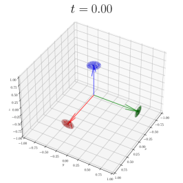
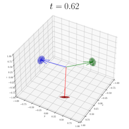
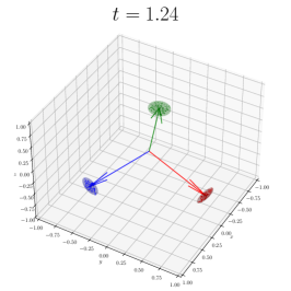
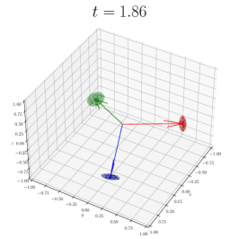
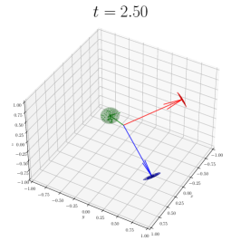
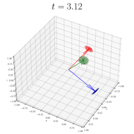
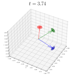
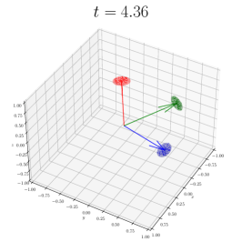
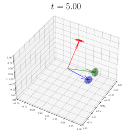
Figure 4: The reachable set for the orientation of a satellite evolving on $SO(3)$ is visualized as uncertainty sets around a coordinate axis. The system (3) is simulated from the initial set $\{I\exp(X):\sqrt{\langle X,X\rangle_{\mathfrak{g}}}\leq 0.1\}$, under the control mapping $\mathbf{u}:[0,5]\to\mathbb{R}^{3}$, $t\mapsto\mathbf{u}(t)=\left[\frac{5-t}{5},1-\left(\frac{t}{5}\right)^{2},\sin\left(\frac{\pi t}{2}\right)\right]^{T}$. Since the system is nonexpansive, and there are no disturbances applied, the reachable set does not grow or shrink over time. $100$ Monte Carlo simulations with initial conditions drawn from this initial set are also shown, verifying their containment in the reachable set.

Discussion After choosing an orthonormal basis for $\mathfrak{g}$, the analysis essentially reduces to analyzing the trivial system $\dot{x}=u$ in Euclidean space. Since we consider a fixed, open-loop control input, every two trajectories always remain the same distance apart. In the same way, on $SO(3)$, just one base trajectory needs to be simulated, and the rest are recoverable by left-translating from this trajectory.

VII CONCLUSIONS

In this work, we specialized existing results in coordinate-free contraction [14] to reductive homogeneous spaces equipped with an invariant Riemannian metric. In these circumstances, we showed how the coordinate-free contraction condition can be expressed globally using a standard matrix measure computation, by lifting the problem to the Lie group. Using this global result, we were able to provide a necessary condition for the existence of a contractive system, involving the underlying geometry rather than purely topological properties. In future work, we plan to further investigate the connection between invariant contraction using the horizontal bundle $\operatorname{Hor}(G)$, horizontal contraction with respect to a horizontal Finsler-Lyapunov function on $G$ [15], and the notion of semi-contraction [26].

References

• [1] Z. Aminzare and E. D. Sontag, “Contraction methods for nonlinear systems: A brief introduction and some open problems,” in 53rd IEEE Conference on Decision and Control.   IEEE, 2014, pp. 3835–3847.
• [2] F. Bullo, Contraction Theory for Dynamical Systems, 1.1 ed.   Kindle Direct Publishing, 2023. [Online]. Available: https://fbullo.github.io/ctds
• [3] A. Davydov and F. Bullo, “Perspectives on contractivity in control, optimization, and learning,” IEEE Control Systems Letters, vol. 8, pp. 2087–2098, 2024.
• [4] A. Pavlov, A. Pogromsky, N. van de Wouw, and H. Nijmeijer, “Convergent dynamics, a tribute to Boris Pavlovich Demidovich,” Systems & Control Letters, vol. 52, no. 3-4, pp. 257–261, 2004.
• [5] W. Lohmiller and J.-J. E. Slotine, “On contraction analysis for non-linear systems,” Automatica, vol. 34, no. 6, pp. 683–696, 1998.
• [6] I. R. Manchester and J.-J. E. Slotine, “Control contraction metrics: Convex and intrinsic criteria for nonlinear feedback design,” IEEE Transactions on Automatic Control, vol. 62, no. 6, pp. 3046–3053, 2017.
• [7] E. D. Sontag, “Contractive systems with inputs,” in Perspectives in Mathematical System Theory, Control, and Signal Processing: A Festschrift in Honor of Yutaka Yamamoto on the Occasion of his 60th Birthday.   Springer, 2010, pp. 217–228.
• [8] A. Davydov, S. Jafarpour, and F. Bullo, “Non-Euclidean contraction theory for robust nonlinear stability,” IEEE Transactions on Automatic Control, vol. 67, no. 12, pp. 6667–6681, 2022.
• [9] P. DeLellis, M. di Bernardo, and G. Russo, “On QUAD, Lipschitz, and contracting vector fields for consensus and synchronization of networks,” IEEE Transactions on Circuits and Systems I: Regular Papers, vol. 58, no. 3, pp. 576–583, 2010.
• [10] G. Russo, M. Di Bernardo, and E. D. Sontag, “A contraction approach to the hierarchical analysis and design of networked systems,” IEEE Transactions on Automatic Control, vol. 58, no. 5, pp. 1328–1331, 2012.
• [11] D. Wu, B. Yi, and I. R. Manchester, “Control contraction metrics on Lie groups,” arXiv preprint arXiv:2403.15264, 2024.
• [12] S. Coogan, “A contractive approach to separable Lyapunov functions for monotone systems,” Automatica, vol. 106, pp. 349–357, 2019.
• [13] S. Jafarpour, A. Davydov, A. Proskurnikov, and F. Bullo, “Robust implicit networks via non-Euclidean contractions,” in Advances in Neural Information Processing Systems, vol. 34, 2021, pp. 9857–9868. [Online]. Available: https://proceedings.neurips.cc/paper_files/paper/2021/file/51a6ce0252d8fa6e913524bdce8db490-Paper.pdf
• [14] J. W. Simpson-Porco and F. Bullo, “Contraction theory on Riemannian manifolds,” Systems & Control Letters, vol. 65, pp. 74–80, 2014. [Online]. Available: https://www.sciencedirect.com/science/article/pii/S016769111400005X
• [15] F. Forni and R. Sepulchre, “A differential Lyapunov framework for contraction analysis,” IEEE transactions on automatic control, vol. 59, no. 3, pp. 614–628, 2013.
• [16] D. Wu and G.-R. Duan, “Further geometric and Lyapunov characterizations of incrementally stable systems on Finsler manifolds,” IEEE Transactions on Automatic Control, vol. 67, no. 10, pp. 5614–5621, 2022.
• [17] D. Wu, “Contraction analysis of nonlinear systems on Riemannian manifolds,” Ph.D. dissertation, Université Paris-Saclay; Harbin Institute of Technology (Chine), 2022.
• [18] K. Nomizu, “Invariant affine connections on homogeneous spaces,” American Journal of Mathematics, vol. 76, no. 1, pp. 33–65, 1954.
• [19] J. Gallier and J. Quaintance, Differential geometry and Lie groups: a computational perspective.   Springer, 2020, vol. 12.
• [20] H. Munthe-Kaas, “High order Runge-Kutta methods on manifolds,” Applied Numerical Mathematics, vol. 29, no. 1, pp. 115–127, 1999.
• [21] C. Mostajeran and R. Sepulchre, “Monotonicity on homogeneous spaces,” Mathematics of Control, Signals, and Systems, vol. 30, pp. 1–25, 2018.
• [22] F. Forni and R. Sepulchre, “Differentially positive systems,” IEEE Transactions on Automatic Control, vol. 61, no. 2, pp. 346–359, 2015.
• [23] C. Mostajeran, “Invariant differential positivity,” Ph.D. dissertation, 2018.
• [24] M. Schlarb, “Covariant derivatives on homogeneous spaces: Horizontal lifts and parallel transport,” The Journal of Geometric Analysis, vol. 34, no. 5, p. 150, 2024.
• [25] A. Harapanahalli and S. Coogan, “Efficient reachable sets on Lie groups using Lie algebra monotonicity and tangent intervals,” arXiv preprint arXiv:2403.16214, 2024.
• [26] S. Jafarpour, P. Cisneros-Velarde, and F. Bullo, “Weak and semi-contraction for network systems and diffusively coupled oscillators,” IEEE Transactions on Automatic Control, vol. 67, no. 3, pp. 1285–1300, 2021.