Estimation of spectral gaps for sparse symmetric matrices

Abstract.

In this paper we propose and analyze an algorithm for identifying spectral gaps of a real symmetric matrix $A$ by simultaneously approximating the traces of spectral projectors associated with multiple different spectral slices. Our method utilizes Hutchinson’s stochastic trace estimator together with the Lanczos algorithm to approximate quadratic forms involving spectral projectors. Instead of focusing on determining the gap between two particular consecutive eigenvalues of $A$, we aim to find all gaps that are wider than a specified threshold. By examining the problem from this perspective, and thoroughly analyzing both the Hutchinson and the Lanczos components of the algorithm, we obtain error bounds that allow us to determine the numbers of Hutchinson’s sample vectors and Lanczos iterations needed to ensure the detection of all gaps above the target width with high probability. In particular, we conclude that the most efficient strategy is to always use a single random sample vector for Hutchinson’s estimator and concentrate all computational effort in the Lanczos algorithm. Our numerical experiments demonstrate the efficiency and reliability of this approach.

1. Introduction

We consider the problem of locating gaps in the spectrum of an $n\times n$ real symmetric matrix $A$, i.e., finding intervals that do not contain any eigenvalue of $A$. A variant of this problem that is more commonly encountered in the literature is the following: given an integer $k$ with $1\leq k<n$, find a real number $\mu$ such that exactly $k$ of the eigenvalues of $A$ (counted with their multiplicities) are strictly below $\mu$. This problem can be equivalently restated as finding $\mu$ such that the spectral projector $P_{\mu}$ onto the subspace spanned by the eigenvectors of $A$ associated with eigenvalues strictly smaller than $\mu$ satisfies $\operatorname{rank}(P_{\mu})=k$; since for a projector the rank is equal to the trace, we can also write this requirement as $\operatorname{tr}(P_{\mu})=k$. If we denote the eigenvalues of $A$ by $\lambda_{i}$ and we label them in non-decreasing order, this problem has a solution only if $\lambda_{k}<\lambda_{k+1}$ (non-degeneracy assumption). In this case, any $\mu$ lying in the open interval $(\lambda_{k},\lambda_{k+1})$ is a solution. Instead of looking for the gap for a specific value of $k$, the approach that we present here aims to find all gaps in the spectrum with width above a certain threshold, and in addition we obtain an estimate of the number of eigenvalues below each gap. In practical cases where it is of interest to find $\mu$ in the gap between $\lambda_{k}$ and $\lambda_{k+1}$, the gap $(\lambda_{k},\lambda_{k+1})$ is usually relatively large, so we expect to be able to find it by looking for all gaps above a certain width.

A major application area where this kind of problem is encountered is electronic structure computations. For example, in Kohn-Sham Density Functional Theory [19] it is required to determine either the eigenvectors of a symmetric matrix $A$ (the discretized Hamiltonian) associated with eigenvalues below the Fermi level (or chemical potential, usually denoted by $\mu$), corresponding to the so-called occupied states of the system, or equivalently the corresponding spectral projector $P_{\mu}$. In the case of insulators at zero electronic temperature, the discrete Hamiltonian $A$ exhibits a gap separating the first $k$ eigenvalues from the rest of the spectrum, where $k$ is the number of electrons, and locating this gap is equivalent to estimating the Fermi level $\mu$. In linear scaling electronic structure computations the spectral projector is approximated either by polynomials or by rational functions that act as filters, i.e., approximate the step function $h_{\mu}(\lambda)$ that takes the value 1 for $\lambda<\mu$ and $0$ for $\lambda>\mu$ (see, e.g., [1]). Clearly, in order to use this approach it is first necessary to estimate the Fermi level $\mu$, which is a nontrivial task.

In the literature, a few approaches have been proposed to estimate values of $\mu$ lying within the target gap. It is well known that for any real symmetric matrix $A-\mu I$ there exists a unit lower triangular matrix $L$ and a block diagonal matrix $D$ with $1\times 1$ and $2\times 2$ blocks such that $A-\mu I=LDL^{T}$; see for example [3, Chapter 1.3.4]. Since $A$ and $D$ are congruent, they have the same inertia, i.e., the same number of positive, negative, and possibly zero eigenvalues (the latter can occur only when $\mu$ happens to be an eigenvalue of $A$, an extremely unlikely occurrence in practice). Hence, if $A$ is not too large, an $LDL^{T}$ factorization of $A-\mu I$ can be used to count the number of eigenvalues smaller than $\mu$. If this number is less than $k$ (larger than $k$) then $\mu$ is increased (respectively, decreased) and the procedure is repeated until the correct value is found. When $A$ is sparse, one can make use of symmetric row and column permutations to reduce the fill-in in $L$ (and therefore the arithmetic and storage costs) while preserving sparsity, see [28, Chapter 7]. A major drawback of this approach is its cost, and especially the fact that having computed the $LDL^{T}$ factorization of $A-\mu I$ for a certain $\mu$ is of no help in computing the factorization for a different value of $\mu$, hence using matrix factorizations in a trial-and-error fashion can be prohibitively expensive, even assuming that a factorization can be computed at all.

Different techniques have been used in the context of linear scaling methods. In these methods, an initial guess $\mu_{0}\approx\mu$ is used in constructing a polynomial approximation to the projector $P_{\mu_{0}}$ by an iterative process known as purification, essentially a Newton-type method. The value of $\mu$ is adjusted in the course of the iterative process until the prescribed value $k$ of the trace is obtained; hence, the determination of $\mu$ and the approximation of the projector $P_{\mu}$ are interweaved. The main cost in this approach is the need to repeatedly solve $n\times n$ linear systems with variable coefficient matrix at each iteration. We refer to [23, 22] for details on these adaptive procedures.

Yet another approach is the one that combines stochastic trace estimators with the Lanczos algorithm to compute an approximation of $\operatorname{tr}(P_{\mu})$. An advantage of this approach is that we can exploit the shift-invariance property of Krylov subspaces (see, e.g., [11]) to efficiently approximate the trace of the spectral projectors $P_{\mu}$ associated with many different values of $\mu$ at the same time. The combination of Hutchinson’s estimator and the Lanczos algorithm has also appeared in literature on related problems that exploit the trace of spectral projectors, such as the estimation of the number of eigenvalues of a matrix $A$ contained in a given interval $[a,b]$ or the estimation of spectral densities, see, for instance, [7, 20]. In the context of spectral density approximation, a similar approach is the kernel polynomial method, which was introduced in [29, 31] and uses a polynomial expansion based on Chebyshev polynomials.

Here we focus on the approach that combines Hutchinson’s trace estimator and the Lanczos algorithm to estimate the trace of the spectral projectors $P_{\mu}$. When using this kind of approach, it is essential to have a criterion to choose the parameters of the algorithm, namely the number of random vectors $\boldsymbol{x}_{i}$ for Hutchinson’s estimator and the number of Lanczos iterations, in order to minimize the computational cost and guarantee the correctness of the results. However, although there exist theoretical results on the convergence speed of this approach, past literature did not give particular attention to establishing how the parameters should be selected. The main purpose of this work is to answer this question for the problem of finding gaps in the spectrum of a matrix. By changing the point of view from finding $\mu$ such that the number of eigenvalues below $\mu$ is exactly $k$ to finding all the gaps in the spectrum with width above a certain threshold, we are able to provide a rigorous analysis that allows us to choose the input parameters to ensure that all the target gaps are found, and at the same time minimize the computational cost. Our analysis will determine that for this problem the most efficient choice is to use a single quadratic form $\boldsymbol{x}^{T}P_{\mu}\boldsymbol{x}$ to approximate $\operatorname{tr}(P_{\mu})$, but in order to reach this conclusion we first have to analyze the more general algorithm that uses Hutchinson’s stochastic trace estimator. This analysis will result in an algorithm that simultaneously computes upper and lower bounds to $\boldsymbol{x}^{T}P_{\mu}\boldsymbol{x}$ for all considered values of $\mu$, and exploits them to find intervals that contain no eigenvalues of $A$ with high probability.

The rest of the paper is organized as follows. In Section 2 we describe a basic version of the algorithm that we are going to use to detect the gaps in the spectrum of $A$. Each component of the algorithm is then analyzed in detail in Section 3, with a focus on bounding the error. Then, in Section 4 we put together the analysis to determine the best choice of input parameters and we obtain an efficient and robust algorithm that can give guarantees on its output. In Section 5 we conduct some numerical experiments to evaluate the performance and reliability of our approach. Finally, Section 6 contains some concluding remarks.

2. Algorithm overview

We start by introducing some notation to establish the framework for our algorithm. Given $\mu\in\mathbb{R}$, let $h_{\mu}:\mathbb{R}\to\mathbb{R}$ denote the Heaviside function

$$h_{\mu}(x)=\begin{cases}1&\text{for $x<\mu$,}\\ 1/2&\text{for $x=\mu$,}\\ 0&\text{for $x>\mu$.}\end{cases}$$

The step function $h_{\mu}$ is closely related to the sign function, indeed we have $h_{\mu}(x)=-\frac{1}{2}\operatorname{sign}(x-\mu)+\frac{1}{2}$. We denote by $\lambda_{i}$ the eigenvalues of $A$ in non-decreasing order, counted according to their multiplicities, and by $\{\boldsymbol{u}_{i}\}_{i=1}^{n}\subset\mathbb{R}^{n}$ an orthonormal basis of eigenvectors, where $\boldsymbol{u}_{i}$ is an eigenvector associated with $\lambda_{i}$. Assuming that $\mu$ does not coincide with any of the eigenvalues of the matrix $A$, we can define the spectral projector

$$P_{\mu}:=h_{\mu}(A)=\sum_{i\,:\,\lambda_{i}<\mu}\boldsymbol{u}_{i}\boldsymbol{u}_{i}^{T}.$$

In the following, we are always going to assume that $\mu\neq\lambda_{i}$ for all $i=1,\dots,n$. Since the eigenvalues of $P_{\mu}$ are all either $0$ or $1$, we have

$$\operatorname{tr}(P_{\mu})=\operatorname{rank}(P_{\mu})=\#\{i\,:\,\lambda_{i}<\mu\}=:\operatorname{n_{e}}(\mu),$$

where $\operatorname{n_{e}}(\mu)$ denotes the number of eigenvalues of $A$ that are strictly smaller than $\mu$. The problem of finding gaps in the spectrum of $A$ can be formulated as finding intervals $[a_{j},b_{j}]$ such that $\operatorname{tr}(P_{\mu})$ is constant for $\mu\in[a_{j},b_{j}]$. We are going to determine gaps in the spectrum of $A$ by approximating $\operatorname{tr}(P_{\mu})$ for several different values of $\mu$, using Hutchinson’s trace estimator combined with the Lanczos method for the approximation of quadratic forms. We first focus on the approximation of $\operatorname{tr}(P_{\mu})$ for a fixed value of $\mu$.

2.1. Hutchinson’s trace estimator

Stochastic trace estimators approximate the trace of a matrix $B$ that is accessible via matrix-vector products by making use of the fact that, for any random vector $\boldsymbol{x}$ such that $\mathbb{E}[\boldsymbol{x}\boldsymbol{x}^{T}]=I$, we have $\mathbb{E}[\boldsymbol{x}^{T}B\boldsymbol{x}]=\operatorname{tr}(B)$, where $\mathbb{E}$ denotes the expected value. Hutchinson’s trace estimator [17] is a simple stochastic estimator that generates $s$ vectors $\boldsymbol{x}_{1},\dots,\boldsymbol{x}_{s}$ with i.i.d. random entries, that are usually chosen as either Gaussian $\mathcal{N}(0,1)$ or Rademacher (uniform $\pm 1$), and approximates $\operatorname{tr}(B)$ with

(2.1) $$\operatorname{tr}^{\mathrm{H}}_{s}(B):=\frac{1}{s}\sum_{i=1}^{s}\boldsymbol{x}_{i}^{T}B\boldsymbol{x}_{i}.$$

In order to attain an absolute accuracy $\varepsilon$ on $\operatorname{tr}(B)$, Hutchinson’s trace estimator requires $O(\lVert B\rVert_{F}^{2}/\varepsilon^{2})$ sample vectors [5, 26]. More precisely, the error from the Hutchinson’s trace estimator when $B$ is symmetric can be bounded by using the following result from [5].

Proposition 2.1 ([5, Theorem 1]).

Let $B$ be a nonzero symmetric matrix, and let $\operatorname{tr}^{\mathrm{H}}_{s}(B)$ denote the Hutchinson trace approximation obtained using $s$ i.i.d. Gaussian $\mathcal{N}(0,1)$ random vectors. If

$$s\geq\frac{4}{\varepsilon^{2}}\big{(}\lVert B\rVert_{F}^{2}+\varepsilon\lVert B\rVert_{2}\big{)}\log(2/\delta),$$

then

$$\mathbb{P}\big{(}\lvert\operatorname{tr}(B)-\operatorname{tr}_{s}^{H}(B)\rvert\geq\varepsilon\big{)}\leq\delta.$$

If we use vectors with Rademacher instead of Gaussian entries, the convergence rate of Hutchinson’s estimator depends on $\lVert B-\operatorname{diag}(B)\rVert_{F}$ and $\lVert B-\operatorname{diag}(B)\rVert_{2}$ instead of $\lVert B\rVert_{F}$ and $\lVert B\rVert_{2}$, so in certain situations it can be faster than with Gaussian vectors, for instance when $B$ is diagonally dominant; see [5, Corollary 1] for a precise statement.

The $O(1/\varepsilon^{2})$ dependence on $\varepsilon$ of the number of sample vectors $s$ makes it very expensive to obtain highly accurate approximations with stochastic trace estimators. However, this is not an issue for a setting such as ours, where an absolute accuracy $\varepsilon=\frac{1}{2}$ is enough to exactly determine $\operatorname{tr}(P_{\mu})$, which is an integer. In contrast, the dependence on $\lVert P_{\mu}\rVert_{F}^{2}$ will make it quite difficult to accurately estimate the number of eigenvalues below $\mu$, since $\lVert P_{\mu}\rVert_{F}^{2}=\operatorname{n_{e}}(\mu)$ can be quite large. Note that when $\mu$ is close to the right endpoint of the spectrum, one can consider $I-P_{\mu}$ instead of $P_{\mu}$ in order to reduce its norm, since $\operatorname{tr}(I-P_{\mu})=n-\operatorname{n_{e}}(\mu)$. To overcome this issue, we will have to slightly change our perspective in order to develop an efficient algorithm. This topic will be discussed in greater detail in Section 3.2. However, this does not handle the case where $\mu$ is near the center of the spectrum. To overcome this issue, we will have to slightly change our perspective in order to develop an efficient algorithm. This topic will be discussed in greater detail in Section 3.2.

Remark 2.2.

Since $\operatorname{rank}(P_{\mu})=\operatorname{n_{e}}(\mu)$ and all the eigenvalues of $P_{\mu}$ are either $0$ or $1$, for this setting it usually does not make much sense to use the improved stochastic trace estimators such as Hutch++ [21, 25] or XTrace [8], which also employ a low-rank matrix approximation. Indeed, there is no gradual decay in the eigenvalues of $P_{\mu}$ and hence there is no advantage in computing a low-rank approximation of $P_{\mu}$, unless $\operatorname{n_{e}}(\mu)$ is very small compared to the matrix size.

Remark 2.3.

When the matrix $A$ is sparse, we could alternatively approximate the trace of the matrix function $P_{\mu}=h_{\mu}(A)$ with a probing method (see, for instance, [13, 2, 12]). The probing approach has a faster convergence when the function $h_{\mu}(A)$ is well-approximated by polynomials on the spectrum of $A$ [13, Theorem 4.4], i.e., it converges similarly to the Lanczos method for the computation of $h_{\mu}(A)\boldsymbol{x}$. We will see in Section 3.3 that this convergence rate is heavily dependent on the value of $\mu$, so we prefer to use a stochastic trace estimator in order to eliminate this dependence.

2.2. Lanczos approximation of quadratic forms

Within Hutchinson’s estimator we have to compute the quadratic forms $\boldsymbol{x}_{i}^{T}P_{\mu}\boldsymbol{x}_{i}$ for $i=1,\dots,s$, which can be done efficiently by using the Lanczos method. For simplicity, consider a single quadratic form $\boldsymbol{x}^{T}h_{\mu}(A)\boldsymbol{x}$. Let us denote by $\mathcal{K}_{m}(A,\boldsymbol{x})=\operatorname{span}\{\boldsymbol{x},A\boldsymbol{x},\dots,A^{m-1}\boldsymbol{x}\}$ the Krylov subspace of dimension $m$ associated to $A$ and $\boldsymbol{x}$, and let $V_{m}\in\mathbb{R}^{n\times m}$ be an orthonormal basis of $\mathcal{K}_{m}(A,\boldsymbol{x})$ constructed using the Lanczos algorithm [27, Algorithm 6.15]. The Lanczos algorithm also constructs a tridiagonal matrix $\underline{T_{m}}\in\mathbb{R}^{(m+1)\times m}$ that satisfies the Arnoldi relation

$$AV_{m}=V_{m+1}\underline{T}_{m}.$$

The quadratic form $\boldsymbol{x}^{T}P_{\mu}\boldsymbol{x}$ can then be approximated with

(2.2) $$\texttt{q}_{m}:=\lVert\boldsymbol{x}\rVert_{2}^{2}\boldsymbol{e}_{1}^{T}h_{\mu}(T_{m})\boldsymbol{e}_{1},$$

where $T_{m}=V_{m}^{T}AV_{m}$ is the leading principal $m\times m$ block of $\underline{T}_{m}$. The convergence rate of the approximation in 2.2 depends on how well the function $f$ can be approximated with polynomials over the spectrum of $A$; see Section 3.3. The Lanczos approximation of $\boldsymbol{x}^{T}P_{\mu}\boldsymbol{x}$ can also be interpreted and analyzed in terms of Gaussian quadrature rules [15].

2.3. Simultaneous computation for different $\mu$

The approach described above can be easily modified in order to compute approximations to $\operatorname{tr}(P_{\mu})$ simultaneously for several $\mu$, for a cost that is only slightly higher than the cost of the approximation for a single $\mu$. The key observation is that for a fixed matrix $A$ and vector $\boldsymbol{x}$, we can extract approximations to the quadratic forms $\boldsymbol{x}^{T}f_{j}(A)\boldsymbol{x}$ for several different functions $f_{j}$ from a single Krylov subspace $\mathcal{K}_{m}(A,\boldsymbol{x})$. Since the cost of computing the approximation 2.2 is dominated by the cost of constructing the orthonormal basis $V_{m}$ via the Lanczos algorithm, the additional operations required to compute approximations for different functions represent only a minor part of the overall cost. More precisely, let us consider $N_{f}$ different functions $f_{j}$, $j=1,\dots,N_{f}$. For a fixed Krylov subspace dimension $m$, we can approximate each quadratic form $\boldsymbol{x}^{T}f_{j}(A)\boldsymbol{x}$ with

$$\texttt{q}_{m,j}:=\lVert\boldsymbol{x}\rVert_{2}^{2}\boldsymbol{e}_{1}^{T}f_{j}(T_{m})\boldsymbol{e}_{1},\qquad j=1,\dots,N_{f}.$$

The quantities $\texttt{q}_{m,j}$ can be computed efficiently in the following way. Obtain first an eigenvalue decomposition $T_{m}=U_{m}^{T}D_{m}U_{m}$ and compute $f_{j}(D_{m})$ for $j=1,\dots,N_{f}$ by applying the functions $f_{j}$ to the diagonal entries of $D_{m}$. The Lanczos approximations to the quadratic forms can now be computed with the identity

$$\texttt{q}_{m,j}=\boldsymbol{w}_{m}^{T}f_{j}(D_{m})\boldsymbol{w}_{m},\qquad j=1,\dots,N_{f},$$

where $\boldsymbol{w}_{m}:=\lVert\boldsymbol{x}\rVert_{2}U_{m}\boldsymbol{e}_{1}$ is the same for all $j$ and needs to be computed only once. If we assume that the small matrix function $f(T_{m})$ is computed via an eigenvalue decomposition also in the case of a single function $f$, the only additional operations that we have to do when we have $N_{f}$ different functions are the computation of the diagonal matrix functions $f_{j}(D_{m})$ and the computation of the final approximations $\texttt{q}_{m,j}=\boldsymbol{w}_{m}^{T}f_{j}(D_{m})\boldsymbol{w}_{m}$ for all $j$, for a total cost of $O(mN_{f})$. This additional cost is negligible compared to the $O(m\,\texttt{nnz}(A))$ cost for the matrix-vector products with $A$ in the construction of the Krylov subspace $\mathcal{K}_{m}(A,\boldsymbol{x})$, unless the number of functions $N_{f}$ is extremely large.

In total, the cost of computing approximations to $\boldsymbol{x}^{T}f_{j}(A)\boldsymbol{x}$ for $j=1,\dots,N_{f}$ with the Lanczos algorithm adds up to $O(m\,\texttt{nnz}(A)+nm+m^{3}+mN_{f})$, where the $O(nm)$ term is the cost of orthogonalization in the Lanczos algorithm using the three-term recurrence; if full reorthogonalization is used instead to increase stability, the orthogonalization cost would increase to $O(nm^{2})$. The $O(m^{3})$ term corresponds to the computation of eigenvalues and eigenvectors of the tridiagonal matrix $T_{m}$, and the $O(mN_{f})$ term corresponds to the computation of $\texttt{q}_{m,j}$ for all $j$. Note that the convergence rate of the approximation of the quadratic form $\boldsymbol{x}^{T}f_{j}(A)\boldsymbol{x}$ can vary significantly depending on the function $f_{j}$, so this approach may construct approximations with considerably different errors for different functions, since we are using the same number of iterations $m$ for all functions. We will focus on analyzing this aspect in Section 3.3.

Remark 2.4.

A similar approach could be used to approximate quadratic forms with several different functions using rational Krylov methods [16], which depend on a certain sequence of poles $\boldsymbol{\xi}=[\xi_{1},\dots,\xi_{m-1}]$ and employ as an approximation space the rational Krylov subspace $\mathcal{Q}_{m}(A,\boldsymbol{x},\boldsymbol{\xi})=q_{m-1}(A)^{-1}\mathcal{K}_{m}(A,\boldsymbol{b})$, with $q_{m-1}(z):=\prod_{j=1}^{m-1}(z-\xi_{j})$. However, the convergence of a rational Krylov method is heavily dependent on the poles $\boldsymbol{\xi}$, which should be chosen depending on the function. In particular, in the case of $f_{j}=h_{\mu_{j}}$ for different parameters $\mu_{j}$, a sequence of poles that produces an accurate approximation for a certain $\mu_{j}$ will give poor approximations for other parameters, especially if they are far from $\mu_{j}$. For this reason, the Lanczos method is better suited for this scenario. A rational Krylov subspace method could be useful to compute a more accurate approximation for the quadratic form $\boldsymbol{x}^{T}h_{\mu}(A)\boldsymbol{x}$ associated with a specific parameter $\mu$, especially in situations in which the Lanczos method converges very slowly.

Returning now to the approximation of $\operatorname{tr}(P_{\mu})$ with Hutchinson’s estimator, let us consider $N_{f}$ different parameters $\{\mu_{j}\}_{j=1}^{N_{f}}\subset\mathbb{R}$ and define the functions $f_{j}=h_{\mu_{j}}$. Provided that we use the same random sample vectors $\{\boldsymbol{x}_{i}\}_{i=1}^{s}$ for the approximation of $\operatorname{tr}(P_{\mu_{j}})$ via Hutchinson’s estimator for all $j$, we can use the same Krylov subspace $\mathcal{K}_{m}(A,\boldsymbol{x}_{i})$ to extract approximations to $\boldsymbol{x}_{i}^{T}P_{\mu_{j}}\boldsymbol{x}_{i}$ for all $\mu_{j}$ at the same time, with essentially the same cost of approximating a quadratic form for a single parameter $\mu$. This feature of this approach represents a considerable computational advantage over other methods, such as those based on the $LDL^{T}$ factorization, which are only able to test a single candidate $\mu$ at a time.

A high-level algorithmic description of the procedure outlined in this section is given in Algorithm 1. This algorithm returns an approximation to $\operatorname{tr}(P_{\mu_{j}})$ for all $j=1,\dots,N_{f}$. The level of accuracy of these approximations, as well as whether they can be exploited to detect gaps in the spectrum of $A$, is going to be thoroughly investigated in the sections that follow. We are also going to identify criteria for selecting the input parameters of the method, namely the number of Hutchinson sample vectors $s$ and Lanczos iterations $m$. The product of this analysis will be an algorithm that, given as input a failure probability $\delta$ and a relative gap width $\theta$, aims to find all the gaps in the spectrum whose relative width is larger than $\theta$; each one of these gaps is found with probability at least $1-\delta$. In addition, all the gaps found by the algorithm are certified, in the sense that the probability of finding an eigenvalue of $A$ within a gap is smaller than $\delta$.

Algorithm 1 Eigenvalue gap finder – Prototype

1:Symmetric matrix $A\in\mathbb{R}^{n\times n}$, number of Hutchinson samples $s$, Krylov subspace dimension $m$, vector of test parameters $\boldsymbol{\mu}=[\mu_{1},\dots,\mu_{N_{f}}]$

2:$\texttt{tr}_{j}\approx\operatorname{tr}(P_{\mu_{j}})$ for $j=1,\dots,N_{f}$

3:for $i=1,\dots,s$ do

4:     Draw a vector $\boldsymbol{x}_{i}\in\mathbb{R}^{n}$ with random i.i.d. Gaussian $\mathcal{N}(0,1)$ entries

5:     Construct an orthonormal basis $V_{m}\in\mathbb{R}^{n\times m}$ of the Krylov space $\mathcal{K}_{m}(A,\boldsymbol{x}_{i})$ with the Lanczos algorithm and compute the associated tridiagonal matrix $\underline{T}_{m}\in\mathbb{R}^{(m+1)\times m}$

6:     Compute the eigenvalue decomposition $T_{m}=U_{m}^{T}D_{m}U_{m}$ and $\boldsymbol{w}_{m}=\lVert\boldsymbol{x}_{i}\rVert_{2}U_{m}\boldsymbol{e}_{1}$

7:     for $j=1,\dots,N_{f}$ do

8:         Compute $\texttt{q}_{m,j}^{(i)}=\boldsymbol{w}_{m}^{T}h_{\mu_{j}}(D_{m})\boldsymbol{w}_{m}$

9:     end for

10:end for

11:for  $j=1,\dots,N_{f}$  do

12:     Compute the trace approximation $\texttt{tr}_{j}=s^{-1}\sum_{i=1}^{s}\texttt{q}_{m,j}^{(i)}$

13:end for

3. Algorithm analysis

In this section we examine some general properties of the trace approximations computed by Algorithm 1, and we analyze in detail the errors that occur in the Hutchinson and Lanczos parts of the approximation.

3.1. General properties

A simple but essential observation is that the approximations to $\operatorname{tr}(P_{\mu})$ computed by Algorithm 1 are increasing in $\mu$. Let us start by looking at the Hutchinson approximation. Denoting by $(\lambda_{j},\boldsymbol{u}_{j})_{j=1}^{n}$ the normalized eigenpairs of $A$, so that $A=\sum_{j=1}^{n}\lambda_{j}\boldsymbol{u}_{j}\boldsymbol{u}_{j}^{T}$, we can write the trace approximation obtained with Hutchinson’s estimator as

$$\operatorname{tr}^{\mathrm{H}}_{s}(P_{\mu})=\frac{1}{s}\sum_{i=1}^{s}\boldsymbol{x}_{i}^{T}P_{\mu}\boldsymbol{x}_{i}=\frac{1}{s}\sum_{i=1}^{s}\boldsymbol{x}_{i}^{T}\Big{(}\sum_{j\,:\,\lambda_{j}<\mu}\boldsymbol{u}_{j}\boldsymbol{u}_{j}^{T}\Big{)}\boldsymbol{x}_{i}=\frac{1}{s}\sum_{i=1}^{s}\sum_{j\,:\,\lambda_{j}<\mu}\lvert\boldsymbol{u}_{j}^{T}\boldsymbol{x}_{i}\rvert^{2}.$$

This shows that the Hutchinson trace approximation is monotonic in $\mu$. In addition, the above identity also highlights the fact that Hutchinson’s approximation of $\operatorname{tr}(P_{\mu})$ is a piecewise constant function, with jumps when $\mu$ coincides with an eigenvalue of $A$. The height of the jump at $\lambda_{k}$ is given by $\frac{1}{s}\sum_{i=1}^{s}\lvert\boldsymbol{u}_{k}^{T}\boldsymbol{x}_{i}\rvert^{2}$.

Let us now consider the Lanczos approximation of the quadratic form $\boldsymbol{x}_{i}^{T}P_{\mu}\boldsymbol{x}_{i}$. Letting $T_{m}^{(i)}$ be the projection of $A$ onto $\mathcal{K}_{m}(A,\boldsymbol{x}_{i})$ computed by the Lanczos algorithm, and denoting by $(\lambda_{j}^{(i)},\boldsymbol{u}_{j}^{(i)})_{j=1}^{m}$ the normalized eigenpairs of $T_{m}^{(i)}$, we have

$$\boldsymbol{x}_{i}^{T}P_{\mu}\boldsymbol{x}_{i}\approx\texttt{q}_{m,j}^{(i)}:=\lVert\boldsymbol{x}_{i}\rVert_{2}^{2}\boldsymbol{e}_{1}^{T}h_{\mu}(T_{m}^{(i)})\boldsymbol{e}_{1}=\lVert\boldsymbol{x}_{i}\rVert_{2}^{2}\sum_{j\,:\,\lambda_{j}^{(i)}<\mu}\lvert\boldsymbol{e}_{1}^{T}\boldsymbol{u}_{j}^{(i)}\rvert^{2}.$$

Again, this is an increasing function of $\mu$, with jumps whenever $\mu$ coincides with an eigenvalue of $T_{m}^{(i)}$. It follows that the approximation of $\operatorname{tr}(P_{\mu})$ computed by Algorithm 1 using Hutchinson’s estimator and the Lanczos method is an increasing function of $\mu$, with jumps when $\mu$ is equal to an eigenvalue of $T_{m}^{(i)}$ for some $i$.

Example 3.1.

To illustrate the behavior of the approximation of $\operatorname{tr}(P_{\mu})$ computed by Algorithm 1 on a simple example, we consider a symmetric matrix $A$ of size $n=600$, with eigenvalues contained in the interval $[0,60]$ and three gaps given by the intervals $[20,21]$, $[30,32]$ and $[40,44]$. In Figure 1 we compare the approximation from Algorithm 1 with $m=50$ Lanczos iterations, Hutchinson’s estimator $\operatorname{tr}^{\mathrm{H}}_{s}(P_{\mu})$ with exact quadratic forms, and the exact trace $\operatorname{tr}(P_{\mu})$, which coincides with $\operatorname{n_{e}}(\mu)$, for several different values of $\mu$. The number of random vectors is either $s=1$ or $s=10$. Figure 1 confirms the behavior described above. In particular, we see that Hutchinson’s estimator with exact quadratic forms has a jump whenever $\mu$ coincides with an eigenvalue of $A$, so it correctly detects all the gaps in the spectrum, although the value of the approximation of $\operatorname{tr}(P_{\mu})$ can be quite off, especially with $s=1$. On the other hand, Hutchinson’s estimator combined with the Lanczos algorithm for computing quadratic forms, which is the approximation that we are actually able to compute, has jumps when $\mu$ corresponds to an eigenvalue of one of the projected matrices $T_{m}^{(i)}$. We see that the Lanczos approximation is able to detect the largest gap quite well, but the other two gaps do not stand out from the other steps in the staircase-like curve. With $s=10$, the Lanczos curve looks like a staircase with somewhat jagged steps, because the projected matrices $T_{m}^{(i)}$ have different eigenvalues for different random vectors $\boldsymbol{x}_{i}$, and the curve is obtained by averaging the approximations $\texttt{q}_{m,j}^{(i)}$ associated with each $T_{m}^{(i)}$.

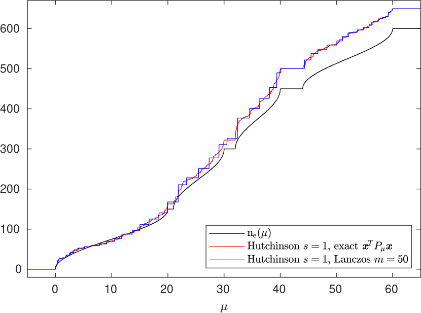
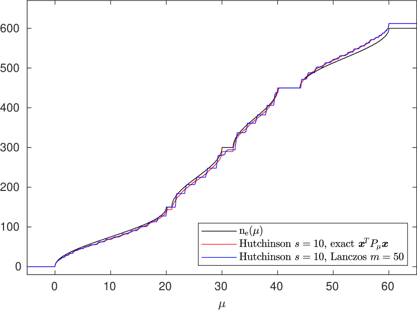
Figure 1. Approximations to $\operatorname{tr}(P_{\mu})$ obtained with Algorithm 1 compared with exact $\operatorname{tr}(P_{\mu})$ and Hutchinson’s approximation $\operatorname{tr}^{\mathrm{H}}_{s}(P_{\mu})$ with exact quadratic forms, for several different $\mu$. Left: $s=1$, $m=50$. Right: $s=10$, $m=50$.

3.2. Trace estimator analysis

In this section we focus on analyzing the approximation of $\operatorname{tr}(P_{\mu})$ using Hutchinson’s estimator. The error from the stochastic trace estimator can be bounded with Proposition 2.1. Since all the eigenvalues of $P_{\mu}$ are either $0$ or $1$, we have $\lVert P_{\mu}\rVert_{2}=1$ and $\lVert P_{\mu}\rVert_{F}^{2}=\operatorname{n_{e}}(\mu)$. Therefore, in order to have $\mathbb{P}\big{(}\lvert\operatorname{tr}(P_{\mu})-\operatorname{tr}_{p}^{H}(P_{\mu})\rvert\geq\varepsilon\big{)}\leq\delta$ with Gaussian vectors, we would need to take

(3.1) $$s\geq\frac{4}{\varepsilon^{2}}\big{(}\operatorname{n_{e}}(\mu)+\varepsilon\big{)}\log(2/\delta).$$

Since the exact $\operatorname{tr}(P_{\mu})$ only takes integer values, in order to compute it correctly it is sufficient to have a final absolute accuracy smaller than $\frac{1}{2}$ on the trace approximation; if we also account for the error in the Lanczos approximation, it is enough to take $\varepsilon=\frac{1}{4}$. However, a key issue with this approach is the fact that the required number of sample vectors $s$ grows proportionally to the number $\operatorname{n_{e}}(\mu)$ of eigenvalues below the level $\mu$. This means that in a situation in which a gap is not close to the extrema of the spectrum, such as if $\operatorname{n_{e}}(\mu)=n/c$ for some moderate constant $c>1$, we would have to take $s=O(n)$, which is too expensive to be practical.

Remark 3.1.

In alternative to Gaussian random vectors, we can also use Rademacher vectors, which have random $\pm 1$ entries. As we mentioned in Section 2.1, the convergence rate of Hutchinson’s estimator with Rademacher random vectors depends on $\lVert B-\operatorname{diag}(B)\rVert_{F}^{2}$ instead of $\lVert B\rVert_{F}^{2}$, so it can be faster than with Gaussian vectors in certain scenarios, such as when the entries of $B$ decay away from the diagonal. Here we prefer to employ Gaussian vectors because of the rotational invariance of their distribution, which will prove useful in the following analysis.

In order to circumvent the growth of the number of sample vectors with $\operatorname{n_{e}}(\mu)$, we slightly change our point of view. Instead of considering the approximation of $\operatorname{tr}(P_{\mu})$, let us take two different values $\mu<\mu^{\prime}$, and consider the difference $\operatorname{tr}(P_{\mu^{\prime}})-\operatorname{tr}(P_{\mu})$. If we use the same sample vectors in Hutchinson’s estimator for both $\operatorname{tr}(P_{\mu})$ and $\operatorname{tr}(P_{\mu^{\prime}})$, the difference $\operatorname{tr}^{\mathrm{H}}_{s}(P_{\mu^{\prime}})-\operatorname{tr}^{\mathrm{H}}_{s}(P_{\mu})$ coincides with the Hutchinson approximation of $\operatorname{tr}(P_{\mu^{\prime}}-P_{\mu})$. Since we have $\lVert P_{\mu^{\prime}}-P_{\mu}\rVert_{F}^{2}=\operatorname{n_{e}}(\mu^{\prime})-\operatorname{n_{e}}(\mu)$, this means that Hutchinson’s estimator can easily approximate the differences in the traces of projectors when $\mu$ and $\mu^{\prime}$ are close enough that there are only a few eigenvalues of $A$ in the interval $[\mu,\mu^{\prime}]$, even if the exact values of $\operatorname{tr}(P_{\mu})$ and $\operatorname{tr}(P_{\mu^{\prime}})$ are quite far from the approximations computed by the stochastic estimator. In particular, the heights of the jumps in $\operatorname{tr}^{\mathrm{H}}_{s}(P_{\mu})$ that occur when $\mu$ coincides with an eigenvalue of $A$ should be approximated quite accurately even with a small number of sample vectors.

Let us analyze this phenomenon in more detail. Recall that

$$\operatorname{tr}^{\mathrm{H}}_{s}(P_{\mu})=\frac{1}{s}\sum_{i=1}^{s}\sum_{j\,:\,\lambda_{j}<\mu}\lvert\boldsymbol{u}_{j}^{T}\boldsymbol{x}_{i}\rvert^{2},$$

so if we take $\mu$ and $\mu^{\prime}$ such that $\lambda_{k-1}<\mu<\lambda_{k}<\mu^{\prime}<\lambda_{k+1}$ for some $k$, we have

$$\operatorname{tr}^{\mathrm{H}}_{s}(P_{\mu^{\prime}})-\operatorname{tr}^{\mathrm{H}}_{s}(P_{\mu})=\frac{1}{s}\sum_{i=1}^{s}\lvert\boldsymbol{u}_{k}^{T}\boldsymbol{x}_{i}\rvert^{2}.$$

Since the random vectors $\boldsymbol{x}_{i}$ are independent of the eigenvector $\boldsymbol{u}_{k}$, we have that $\{\boldsymbol{u}_{k}^{T}\boldsymbol{x}_{i}\}_{i=1}^{s}$ are i.i.d. $\mathcal{N}(0,1)$ random variables, due to the rotational invariance of Gaussian vectors. As a consequence, the random variable $y_{s}=\sum_{i=1}^{s}\lvert\boldsymbol{u}_{k}^{T}\boldsymbol{x}_{i}\rvert^{2}$ has a $\chi^{2}$ distribution with $s$ degrees of freedom, i.e., it is the sum of the squares of $s$ independent unit normal random variables.

We have $\mathbb{E}[y_{s}]=s$, which means that the expected height of each jump in $\operatorname{tr}^{\mathrm{H}}_{s}(P_{\mu})$ is equal to $1$. Intuitively, the height of a jump in $\operatorname{tr}^{\mathrm{H}}_{s}(P_{\mu})$ is small when the vectors $\boldsymbol{x}_{i}$ are all approximately orthogonal to the eigenvector $\boldsymbol{u}_{k}$, an event that has a small chance of occurring. Since small jumps in $\operatorname{tr}^{\mathrm{H}}_{s}(P_{\mu})$ are more difficult to detect when approximating the quadratic forms in Hutchinson’s estimator via the Lanczos method, it will be useful to have an upper bound on the probability of small jumps. The lemma that follows provides us with such a bound. In the following, we say that the jump in $\operatorname{tr}^{\mathrm{H}}_{s}(P_{\mu})$ at the $k$-th eigenvalue of $A$ is $\varepsilon$-small if its height is smaller than $\varepsilon$, i.e., if $y_{s}\leq s\varepsilon$.

Lemma 3.2.

Given $\delta\in(0,1)$ and $\varepsilon\in(0,1)$, if

$$s\geq\frac{2\log(1/\delta)}{\log(1/\varepsilon)+\varepsilon-1},$$

then we have

$$\mathbb{P}(y_{s}\leq s\varepsilon)\leq\delta,$$

i.e., the jump at $\lambda_{k}$ is $\varepsilon$-small with probability at most $\delta$.

Proof.

To prove this, we use a Chernoff bound on the lower tail of the probability distribution of $y_{s}$. For any $\lambda>0$, we have

(3.2) $$\mathbb{P}(y_{s}\leq s\varepsilon)=\mathbb{P}(e^{-\lambda y_{s}}\geq e^{-\lambda s\varepsilon})\leq\frac{\mathbb{E}[e^{-\lambda y_{s}}]}{e^{-\lambda s\varepsilon}},$$

where the last inequality follows from Markov’s inequality. Since $y_{s}$ is a $\chi^{2}$ random variable with $s$ degrees of freedom, we can write $y_{s}=X_{1}^{2}+\dots+X_{s}^{2}$, where $\{X_{j}\}_{j=1}^{s}$ are i.i.d. $\mathcal{N}(0,1)$ random variables. We have

$$\mathbb{E}[e^{-\lambda X_{j}^{2}}]=\frac{1}{\sqrt{2\pi}}\int_{\mathbb{R}}e^{-\lambda z^{2}}e^{-\frac{1}{2}z^{2}}\mathrm{d}z=\frac{1}{\sqrt{2\pi}}\int_{\mathbb{R}}\frac{1}{\sqrt{1+2\lambda}}e^{-\frac{1}{2}y^{2}}\mathrm{d}y=\frac{1}{\sqrt{1+2\lambda}},$$

where we used the change of variables $y=z\,\sqrt{1+2\lambda}$. It follows that

$$\mathbb{E}[e^{-\lambda y_{s}}]=\mathbb{E}\bigg{[}\prod_{j=1}^{s}e^{-\lambda X_{j}^{2}}\bigg{]}=\mathbb{E}[e^{-\lambda X_{1}^{2}}]^{s}=(1+2\lambda)^{-s/2},$$

and by combining this identity with 3.2 we obtain

(3.3) $$\mathbb{P}(y_{s}\leq s\varepsilon)\leq e^{\lambda s\varepsilon}(1+2\lambda)^{-s/2}\qquad\forall\lambda>0.$$

Taking $\lambda=\frac{1}{2\varepsilon}-\frac{1}{2}$, we get

$$\mathbb{P}(y_{s}\leq s\varepsilon)\leq\big{(}\varepsilon e^{1-\varepsilon}\big{)}^{s/2}.$$

With some simple algebraic manipulations, we conclude that $\mathbb{P}(y_{s}\leq s\varepsilon)\leq\delta$ provided that we take

$$s\geq\frac{2\log(1/\delta)}{\log(1/\varepsilon)+\varepsilon-1}.$$

∎

Note that $\mathbb{P}(y_{s}\leq s\varepsilon)$ is the probability that a jump in $\operatorname{tr}^{\mathrm{H}}_{s}(P_{\mu})$ corresponding to a certain fixed eigenvalue of $A$ is $\varepsilon$-small. Observe that the heights of different jumps in $\operatorname{tr}^{\mathrm{H}}_{s}(P_{\mu})$ are independent, because the quantities $\{\boldsymbol{u}_{k}^{T}\boldsymbol{x}_{i}\}_{i,k}$ are all independent due to the rotational invariance of the $\boldsymbol{x}_{i}$ and the orthogonality of the $\boldsymbol{u}_{k}$, so Lemma 3.2 can also be used to obtain conditions on $s$ that bound the probability of having $\varepsilon$-small jumps associated with several different eigenvalues of $A$. The number of sample vectors $s$ required to have an $\varepsilon$-small jump probability lower than $\delta$ reduces as $\varepsilon$ decreases. At the same time, the number of Lanczos iterations required to approximate the quadratic forms with accuracy of order $\varepsilon$ (and thus manage to detect the jumps in $\operatorname{tr}^{\mathrm{H}}_{s}(P_{\mu}))$ increases as $\varepsilon$ becomes small. In Section 3.3 we obtain some bounds on the Lanczos error, which we will later compare with the $\varepsilon$-small jump probability bound from Lemma 3.2 in order to determine the best choice of parameters for the algorithm.

3.3. Lanczos approximation analysis

In this section we discuss the error in the Lanczos approximation of a quadratic form $\boldsymbol{x}^{T}h_{\mu}(A)\boldsymbol{x}$. Recall that we denote by

$$E_{k}(f,\mathcal{S})=\min_{\deg p\leq k}\max_{z\in\mathcal{S}}|f(z)-p(z)|$$

the best uniform norm error in the approximation of a continuous function $f$ on the compact set $\mathcal{S}\subset\mathbb{R}$ with polynomials of degree up to $k$. If $\texttt{q}_{m}$ denotes the Lanczos approximation to $\boldsymbol{x}^{T}f(A)\boldsymbol{x}$ from the Krylov subspace $\mathcal{K}_{m}(A,\boldsymbol{x})$, we have

(3.4) $$\lvert\boldsymbol{x}^{T}f(A)\boldsymbol{x}-\texttt{q}_{m}\rvert\leq 2\lVert\boldsymbol{x}\rVert_{2}^{2}E_{2m-1}(f,\operatorname{\Lambda}(A)\cup\operatorname{\Lambda}(T_{m})),$$

see, for instance, [4, eq. (1.2)]. Since the function $f=h_{\mu}$ is discontinuous at $\mu$, we have that $E_{2m-1}(h_{\mu},[a,b])$ is always at least $\frac{1}{2}$ if $\mu\in[a,b]$, so we cannot derive meaningful error bounds if we simply consider an interval $[a,b]$ that contains the whole spectrum of $A$. On the other hand, we can obtain bounds on the polynomial approximation error of $h_{\mu}$ on two disjoint intervals, one to the left and one to the right of $\mu$. We start by stating a result for the polynomial approximation of the sign function on the union of two symmetric intervals $[-b,-a]\cup[a,b]$.

Proposition 3.3 ([9, Theorem 1]).

Let $0<a<b$. We have

$$\lim_{m\to\infty}\sqrt{m}\bigg{(}\frac{b+a}{b-a}\bigg{)}^{m}E_{2m+1}(\operatorname{sign},[-b,-a]\cup[a,b])=\frac{b-a}{\sqrt{\pi ab}}.$$

The statement of Proposition 3.3 implies that there exists a constant $C>0$ such that

$$E_{2m+1}(\operatorname{sign},[-b,-a]\cup[a,b])\leq\frac{C}{\sqrt{m}}\bigg{(}\frac{b-a}{b+a}\bigg{)}^{m},$$

and for $m$ large enough we can take

$$C=\frac{b-a}{\sqrt{\pi ab}}+1.$$

Remark 3.4.

In a situation in which the spectrum of $A$ is not symmetric with respect to the origin, using the bound in Proposition 3.3 to bound the error of the Lanczos method for the sign function can yield overly pessimistic results, since it would require us to consider intervals that are much wider than $\operatorname{\Lambda}(A)$. In such a case, it would be more convenient to consider the polynomial approximation of the sign function on a nonsymmetric set. For instance, the asymptotics of $E_{2k+1}(\operatorname{sign},[-a,-1]\cup[1,b])$ for $a\neq b$ have been studied in [10], where the authors generalize Proposition 3.3 to [10, Theorem 1.1]. The result in [10] could be used to obtained more refined error bounds for the Lanczos approximation error, but the complexity of the statement, which involves Green’s functions and integral representations, makes it significantly more difficult to employ in our setting.

We can easily turn Proposition 3.3 into a bound for the step function $h_{\mu}$ for any $\mu\in\mathbb{R}$. Let us define

$$b_{1}:=\lambda_{1}-\mu,\qquad a_{1}:=\lambda_{\operatorname{n_{e}}(\mu)}-\mu,\qquad a_{2}:=\lambda_{\operatorname{n_{e}}(\mu)+1}-\mu,\qquad b_{2}:=\lambda_{n}-\mu,$$

and let

$$a:=\min\{\lvert a_{1}\rvert,\lvert a_{2}\rvert\}\qquad\text{and}\qquad b:=\max\{\lvert b_{1}\rvert,\lvert b_{2}\rvert\}.$$

Note that $\operatorname{\Lambda}(A)\subset[\lambda_{1},\lambda_{\operatorname{n_{e}}(\mu)}]\cup[\lambda_{\operatorname{n_{e}}(\mu)+1},\lambda_{n}]$ and recall that $h_{\mu}(x)=-\frac{1}{2}\operatorname{sign}(x-\mu)+\frac{1}{2}$, so we have

$$E_{2m+1}(h_{\mu},[\lambda_{1},\lambda_{\operatorname{n_{e}}(\mu)}]\cup[\lambda_{\operatorname{n_{e}}(\mu)+1},\lambda_{n}]) =E_{2m+1}(h_{0},[b_{1},a_{1}]\cup[a_{2},b_{2}])$$

$$=\frac{1}{2}E_{2m+1}(\operatorname{sign},[b_{1},a_{1}]\cup[a_{2},b_{2}])$$

$$\leq\frac{1}{2}E_{2m+1}(\operatorname{sign},[-b,-a]\cup[a,b])$$

$$\leq\frac{C}{2\sqrt{m}}\bigg{(}\frac{b-a}{b+a}\bigg{)}^{m},$$

with $C=1\,+\,(b-a)/\sqrt{\pi ab}$, where we used Proposition 3.3 for the last inequality. Denoting the relative spectral gap associated to $\mu$ by $\theta:=a/b$, we obtain

(3.5) $$E_{2m+1}(h_{\mu},[\lambda_{1},\lambda_{\operatorname{n_{e}}(\mu)}]\cup[\lambda_{\operatorname{n_{e}}(\mu)+1},\lambda_{n}])\leq\frac{C}{2\sqrt{m}}\bigg{(}\frac{1-\theta}{1+\theta}\bigg{)}^{m}.$$

We can combine this result with 3.4 to bound the error in the Lanczos approximation of quadratic forms with $P_{\mu}=h_{\mu}(A)$, provided that no eigenvalue of $T_{m}$ lies within the gap $(\lambda_{\operatorname{n_{e}}(\mu)},\lambda_{\operatorname{n_{e}}(\mu)+1})$. Unfortunately, this cannot be excluded a priori; however, since there must be at least one eigenvalue of $A$ in the open interval between two consecutive Ritz values [18, Section 4], there can be at most one eigenvalue of $T_{m}$ in the interval $(\lambda_{\operatorname{n_{e}}(\mu)},\lambda_{\operatorname{n_{e}}(\mu)+1})$. This fact can be proved using the theory of orthogonal polynomials, see, for instance, [14, Theorem 1.21], using the fact that the Ritz values are the zeros of an orthogonal polynomial associated with a Gauss quadrature rule; see, e.g., [15, Theorem 6.2]. In the analysis that follows, we assume for simplicity that there are no Ritz values in the gap $(\lambda_{\operatorname{n_{e}}(\mu)},\lambda_{\operatorname{n_{e}}(\mu)+1})$. We discuss how we can modify our approach to deal with this issue in Remark 3.7.

Remark 3.5.

In the literature, several techniques have been used to obtain approximations to the sign matrix function that circumvent the problem of Ritz values getting arbitrarily close to zero [30], for instance by writing $\operatorname{sign}(z)=z\cdot(z^{2})^{-1/2}$ and constructing an approximation of $(A^{2})^{-1/2}\boldsymbol{x}$ using the Krylov subspace $\mathcal{K}_{m}(A^{2},\boldsymbol{x})$, which ensures that the eigenvalues of the projected matrix are bounded away from $0$, since $A^{2}$ is positive definite as long as $A$ is nonsingular. Alternatively, one can construct an approximation using harmonic Ritz values [24], which are always outside of the interval between the largest negative and the smallest positive eigenvalue of $A$, so they avoid the discontinuity of the sign function. Since in this work our goal is to approximate $\boldsymbol{x}^{T}h_{\mu}(A)\boldsymbol{x}$ for several $\mu$, we opted to use the standard Lanczos approximation 2.2, for which it is very cheap and straightforward to compute approximations for many different functions.

Combining 3.4 with 3.5, we obtain the following bound on the Lanczos approximation error.

Proposition 3.6.

Let $\texttt{q}_{m}$ be the Lanczos approximation 2.2 to $\boldsymbol{x}^{T}h_{\mu}(A)\boldsymbol{x}$ from the Krylov subspace $\mathcal{K}_{m}(A,\boldsymbol{x})$, and assume that there is no eigenvalue of $T_{m}$ in the interval $(\lambda_{\operatorname{n_{e}}(\mu)},\lambda_{\operatorname{n_{e}}(\mu)+1})$. We have

(3.6) $$\lvert\boldsymbol{x}^{T}h_{\mu}(A)\boldsymbol{x}-\texttt{q}_{m}\rvert\leq\frac{C\lVert\boldsymbol{x}\rVert_{2}^{2}}{\sqrt{m-1}}\bigg{(}\frac{1-\theta}{1+\theta}\bigg{)}^{m-1},$$

where $C$ and $\theta$ are defined above.

Note that if we take a different value of $\mu$ in the interval $(\lambda_{\operatorname{n_{e}}(\mu)},\lambda_{\operatorname{n_{e}}(\mu)+1})$, the error $\lvert\boldsymbol{x}^{T}h_{\mu}(A)\boldsymbol{x}-\texttt{q}_{m}\rvert$ remains the same, because the function $h_{\mu}$ takes the same values on the eigenvalues of $A$ and $T_{m}$ and hence the matrix functions $h_{\mu}(A)$ and $h_{\mu}(T_{m})$ do not change. On the other hand, the bound in Proposition 3.6 depends on $\theta$, which in turn depends on $\mu$. It is quite easy to see that the largest value of $\theta$ is obtained when $\mu$ is precisely in the middle of the gap, i.e. $\mu=\frac{1}{2}(\lambda_{\operatorname{n_{e}}(\mu)}+\lambda_{\operatorname{n_{e}}(\mu)+1})$. This value of $\mu$ gives us the sharpest bound in 3.6.

The convergence predicted by Proposition 3.6 is at least exponential with rate $(1-\theta)/(1+\theta)$, with in addition an $O(1/\sqrt{m})$ factor which is independent of the gap width. Note that the constant $C$ grows as the gap becomes smaller; see Proposition 3.3. In order to have an error $\lvert\boldsymbol{x}^{T}h_{\mu}(A)\boldsymbol{x}-\texttt{q}_{m}\rvert\leq\varepsilon$, the number of Lanczos iterations $m$ should satisfy

(3.7) $$m+\frac{\log(m-1)}{2\log\big{(}(1+\theta)/(1-\theta)\big{)}}\geq 1+\frac{\log\big{(}C\lVert\boldsymbol{x}\rVert_{2}^{2}/\varepsilon\big{)}}{\log\big{(}(1+\theta)/(1-\theta)\big{)}}.$$

Assuming that the relative gap $\theta$ is large enough, we do not lose much by discarding the $\log(m-1)$ term, and we can take

(3.8) $$m\geq 1+\frac{\log\big{(}C\lVert\boldsymbol{x}\rVert_{2}^{2}/\varepsilon\big{)}}{\log\big{(}(1+\theta)/(1-\theta)\big{)}}.$$

On the other hand, in a situation where the spectral gap is very small, the Lanczos method effectively converges like $O(1/\sqrt{m})$. Note that if $\boldsymbol{x}$ is a Gaussian random vector we have $\mathbb{E}[\lVert\boldsymbol{x}\rVert_{2}^{2}]=n$, so with a very small gap for which $\theta\approx 0$ we would need to take

$$m\gtrsim\frac{C^{2}n^{2}}{\varepsilon^{2}},$$

which is definitely unfeasible. This means that when using the Lanczos method we can only hope to approximate $\boldsymbol{x}^{T}h_{\mu}(A)\boldsymbol{x}$ accurately when $\mu$ is inside a relatively large gap in the spectrum of $A$, and we should instead expect to have quite a large error whenever $\mu$ is close to an eigenvalue of $A$.

A crucial requirement for using the bound in Proposition 3.6 is the knowledge of the relative gap width $\theta$. Since the gaps in the spectrum are not known to us in advance, we cannot use this result to check if the error of the Lanczos method is below a certain tolerance $\varepsilon$. On the other hand, Proposition 3.6 can be useful to choose the number $m$ of Lanczos iterations at the start of the algorithm. Indeed, if our goal is to find all the gaps in the spectrum of $A$ with relative width at least $\theta$, for any given $\varepsilon$ we can select $m$ using 3.8 to ensure that the error $\lvert\boldsymbol{x}^{T}h_{\mu}(A)\boldsymbol{x}-\texttt{q}_{m}\rvert\leq\varepsilon$ whenever $\mu$ is inside a gap with width at least $\theta$. However, we are still unable to determine for which values of $\mu$ this condition is satisfied. The final component that we need to make the algorithm work is an a posteriori bound on the error, which will allow us to detect when $\lvert\boldsymbol{x}^{T}h_{\mu}(A)\boldsymbol{x}-\texttt{q}_{m}\rvert\leq\varepsilon$, without knowing the gaps in the spectrum in advance. For this purpose we can use an a posteriori error bound from [2], which we adapt to the step function $h_{\mu}$ in Section 3.4.

Remark 3.7.

If there is an eigenvalue of $T_{m}$ inside the gap $(\lambda_{\operatorname{n_{e}}(\mu)},\lambda_{\operatorname{n_{e}}(\mu)+1})$, the results above do not hold. However, if the gap in the spectrum of $A$ has relative width $\theta$, then there must be a corresponding gap in $\operatorname{\Lambda}(A)\cup\operatorname{\Lambda}(T_{m})$ with a relative width at least $\theta/2$, since there is at most one Ritz value contained in the interval $(\lambda_{\operatorname{n_{e}}(\mu)},\lambda_{\operatorname{n_{e}}(\mu)+1})$. In other words, there is an interval of relative width $\theta/2$ where there are no eigenvalues of $A$ or $T_{m}$, and hence when $\mu$ is inside that interval the Lanczos approximation error satisfies the bound 3.6 with $\theta$ replaced by $\theta/2$.

3.4. An a posteriori error bound for the Lanczos algorithm

In this section we adapt an a posteriori error bound given in [2] for the approximation of $\boldsymbol{x}^{T}f(A)\boldsymbol{x}$ with a rational Krylov method to the case of the Lanczos approximation of $f=h_{\mu}$. The result given in [2, Theorem 4.8] employs the Cauchy integral formula and the residue theorem to obtain upper and lower bounds on the error in the approximation of $\boldsymbol{x}^{T}f(A)\boldsymbol{x}$ with a rational Krylov method. This result can be easily used to bound the error in the Lanczos approximation for $f=h_{\mu}$, but it requires some caution since the function $h_{\mu}$ is discontinuous at $\mu$. In the following, we briefly retrace the proof of [2, Theorem 4.8] and adapt it to the current setting.

If $\Gamma\subset\mathbb{C}$ is a simple closed curve that surrounds the eigenvalues of $A$ below $\mu$, we have

$$P_{\mu}=h_{\mu}(A)=\frac{1}{2\pi i}\int_{\Gamma}(zI-A)^{-1}\mathrm{d}z.$$

If the eigenvalues of $T_{m}$ that are smaller than $\mu$ also lie in the interior of $\Gamma$, we have

$$h_{\mu}(A)\boldsymbol{x}-\lVert\boldsymbol{x}\rVert_{2}V_{m}h_{\mu}(T_{m})\boldsymbol{e}_{1}=\frac{1}{2\pi i}\int_{\Gamma}(zI-A)^{-1}\boldsymbol{r}_{m}(z)\mathrm{d}z,$$

where

$$\boldsymbol{r}_{m}(z)=\boldsymbol{x}-(zI-A)\boldsymbol{x}_{m}(z),\qquad\text{with}\qquad\boldsymbol{x}_{m}(z)=\lVert\boldsymbol{x}\rVert_{2}V_{m}(zI-T_{m})^{-1}\boldsymbol{e}_{1},$$

that is, $\boldsymbol{r}_{m}(z)$ is the residual of a shifted linear system after $m$ iterations of the Lanczos method. With the same algebraic manipulations used in [2, Section 4.3], we obtain

$$\boldsymbol{x}^{T}h_{\mu}(A)\boldsymbol{x}-\lVert\boldsymbol{x}\rVert_{2}^{2}\boldsymbol{e}_{1}^{T}h_{\mu}(T_{m})\boldsymbol{e}_{1}=\frac{\lVert\boldsymbol{x}\rVert_{2}^{2}}{2\pi i}\int_{\Gamma}\varphi_{m}(z)^{2}\boldsymbol{v}_{m+1}^{T}(zI-A)^{-1}\boldsymbol{v}_{m+1}\mathrm{d}z,$$

with

$$\varphi_{m}(z)=t_{m+1,m}\boldsymbol{e}_{m}^{T}(zI-T_{m})^{-1}\boldsymbol{e}_{1},$$

where $t_{m+1,m}$ denotes the element in position $(m+1,m)$ of the matrix $\underline{T}_{m}$. Using an eigenvalue decomposition $T_{m}=U_{m}D_{m}U_{m}^{T}$, with $U_{m}$ orthogonal and $D_{m}=\operatorname{diag}(\theta_{1},\dots,\theta_{m})$, we can define

$$\begin{bmatrix}\alpha_{1},\dots,\alpha_{m}\end{bmatrix}:=t_{m+1,m}\boldsymbol{e}_{m}^{T}U_{m},\qquad\begin{bmatrix}\beta_{1},\dots,\beta_{m}\end{bmatrix}^{T}:=U_{m}^{T}\boldsymbol{e}_{1}$$

and

$$\gamma_{j}:=\sum_{k\,:\,k\neq j}\alpha_{k}\beta_{k}\frac{1}{\theta_{j}-\theta_{k}},\qquad j=1,\dots,m.$$

With these definitions, the function $\varphi_{m}(z)^{2}$ can be rewritten in the form

$$\varphi_{m}(z)^{2}=\sum_{j=1}^{m}\alpha_{j}^{2}\beta_{j}^{2}\frac{1}{(z-\theta_{j})^{2}}+2\sum_{j=1}^{m}\alpha_{j}\beta_{j}\gamma_{j}\frac{1}{z-\theta_{j}}.$$

Using the residue theorem, with the same procedure used in [2, Section 4.3] we obtain

(3.9) $$\boldsymbol{x}^{T}h_{\mu}(A)\boldsymbol{x}-\lVert\boldsymbol{x}\rVert_{2}^{2}\boldsymbol{e}_{1}^{T}h_{\mu}(T_{m})\boldsymbol{e}_{1}=\lVert\boldsymbol{x}\rVert_{2}^{2}\boldsymbol{v}_{m+1}^{T}g_{m}(A)\boldsymbol{v}_{m+1},$$

with

(3.10) $$g_{m}(z):=\begin{cases}\displaystyle\sum_{j\,:\,\theta_{j}>\mu}\alpha_{j}^{2}\beta_{j}^{2}\dfrac{1}{(z-\theta_{j})^{2}}+2\alpha_{j}\beta_{j}\gamma_{j}\dfrac{1}{z-\theta_{j}}&\text{if $z<\mu$,}\\ -\displaystyle\sum_{j\,:\,\theta_{j}<\mu}\alpha_{j}^{2}\beta_{j}^{2}\dfrac{1}{(z-\theta_{j})^{2}}-2\alpha_{j}\beta_{j}\gamma_{j}\dfrac{1}{z-\theta_{j}}&\text{if $z>\mu$.}\end{cases}$$

We can use 3.9 to obtain the following upper bound for the Lanczos approximation error, which corresponds to the upper bound in [2, Theorem 4.8].

Proposition 3.8.

Let $\texttt{q}_{m}$ be the Lanczos approximation 2.2 to $\boldsymbol{x}^{T}h_{\mu}(A)\boldsymbol{x}$ from the Krylov subspace $\mathcal{K}_{m}(A,\boldsymbol{x})$. We have

$$\lvert\boldsymbol{x}^{T}h_{\mu}(A)\boldsymbol{x}-\texttt{q}_{m}\rvert\leq\lVert\boldsymbol{x}\rVert_{2}^{2}\max_{z\in\operatorname{\Lambda}(A)}{\lvert g_{m}(z)\rvert}\leq\lVert\boldsymbol{x}\rVert_{2}^{2}\max_{z\in[\lambda_{\min},\lambda_{\max}]}{\lvert g_{m}(z)\rvert},$$

where $g_{m}$ is defined in 3.10.

In contrast with what happens when the function $f$ is continuous over the whole spectral interval of $A$, in this case the function $g_{m}(z)$ is discontinuous at $\mu$ and the lower bound from [2, Theorem 4.8] no longer holds. Indeed, if we denote by $(\lambda_{k},\boldsymbol{u}_{k})$ the normalized eigenpairs of the matrix $A$, we can write

$$\boldsymbol{v}_{m+1}^{T}g_{m}(A)\boldsymbol{v}_{m+1}=\sum_{k=1}^{m}g_{m}(\lambda_{k})(\boldsymbol{u}_{k}^{T}\boldsymbol{v}_{m+1})^{2},\qquad\text{with}\qquad\sum_{k=1}^{m}(\boldsymbol{u}_{k}^{T}\boldsymbol{v}_{m+1})^{2}=1.$$

This expression shows that the quadratic form $\boldsymbol{v}_{m+1}^{T}g_{m}(A)\boldsymbol{v}_{m+1}$ can potentially take any value in the convex hull of the set $\{g_{m}(\lambda_{k})\}_{k=1}^{m}$, depending on the coefficients $(\boldsymbol{u}_{k}^{T}\boldsymbol{v}_{m+1})^{2}$. In the case that $g_{m}(\lambda_{k})$ takes both positive and negative values, it is possible to have $\boldsymbol{v}_{m+1}^{T}g_{m}(A)\boldsymbol{v}_{m+1}=0$, so the lower bound

$$\lvert\boldsymbol{x}^{T}h_{\mu}(A)\boldsymbol{x}-\lVert\boldsymbol{x}\rVert_{2}^{2}\boldsymbol{e}_{1}^{T}h_{\mu}(T_{m})\boldsymbol{e}_{1}\rvert\geq\lVert\boldsymbol{x}\rVert_{2}^{2}\min_{z\in[\lambda_{\min},\lambda_{\max}]}{\lvert g_{m}(z)\rvert}$$

may not hold. Note that this argument is not in contradiction with the statement of [2, Theorem 4.8] when the function $g_{m}$ is continuous over the whole spectral interval of $A$, because if $g_{m}(\lambda_{k})$ takes both negative and positive values there must be a point $z\in[\lambda_{\min},\lambda_{\max}]$ such that $g_{m}(z)=0$ by continuity of $g_{m}$.

Example 3.2.

In this example we compare the error of the Lanczos approximation of $\boldsymbol{x}^{T}h_{\mu}(A)\boldsymbol{x}$ with the a priori error bound from Proposition 3.6, the a posteriori error bound form Proposition 3.8, and the simple error estimate $\lvert\boldsymbol{x}^{T}h_{\mu}(A)\boldsymbol{x}-\texttt{q}_{m}\rvert\approx\lvert\texttt{q}_{m}-\texttt{q}_{m+1}\rvert$. We consider a symmetric matrix $A$ of size $n=1000$ with $\operatorname{\Lambda}(A)\subset[0,40]$, and gaps in the intervals $[10,11]$ and $[20,25]$. We plot the convergence of the Lanczos method in Figure 2, where on the left plot $\mu=22$ is contained in the larger gap, and on the right plot $\mu=10.6$ is inside the smaller gap. In the legend, the “central $\mu$” a priori bound refers to the bound obtained by taking $\mu$ in the middle of the gap, as mentioned below Proposition 3.6.

Note that the convergence of the Lanczos method is much slower when $\mu$ is inside the smaller gap, and in both cases the convergence behavior is irregular and oscillating. The “central $\mu$” is the most accurate between the two a priori bounds, but it does not capture the correct convergence rate for $\mu=10.6$, which is further from the middle of the spectrum; in this case, a better a priori bound would be obtained by using a convergence result with nonsymmetric intervals, such as [10, Theorem 1.1]. The a posteriori bound is also quite irregular, but it is able to capture the convergence rate of the Lanczos approximation correctly in both cases, although it is off by a constant factor. Surprisingly, the error estimate $\lvert\boldsymbol{x}^{T}h_{\mu}(A)\boldsymbol{x}-\texttt{q}_{m}\rvert\approx\lvert\texttt{q}_{m}-\texttt{q}_{m+1}\rvert$ is very accurate, and it seems to almost never underestimate the error. This behavior can be explained in the following way: the error estimate based on consecutive differences satisfies the triangle inequality

$$\lvert\texttt{q}_{m}-\texttt{q}_{m+1}\rvert\geq\left\lvert\,\lvert\boldsymbol{x}^{T}h_{\mu}(A)\boldsymbol{x}-\texttt{q}_{m}\rvert-\lvert\boldsymbol{x}^{T}h_{\mu}(A)\boldsymbol{x}-\texttt{q}_{m+1}\rvert\,\right\rvert,$$

and due to the oscillations in the convergence of the Lanczos approximation, the two right-hand side terms $\lvert\boldsymbol{x}^{T}h_{\mu}(A)\boldsymbol{x}-\texttt{q}_{m}\rvert$ and $\lvert\boldsymbol{x}^{T}h_{\mu}(A)\boldsymbol{x}-\texttt{q}_{m+1}\rvert$ often have significantly different moduli, so we have

(3.11) $$\left\lvert\,\lvert\texttt{q}-\texttt{q}_{m}\rvert-\lvert\texttt{q}-\texttt{q}_{m+1}\rvert\,\right\rvert\geq c\max\left\{\lvert\texttt{q}-\texttt{q}_{m}\rvert,\lvert\texttt{q}-\texttt{q}_{m+1}\rvert\right\},\qquad\texttt{q}:=\boldsymbol{x}^{T}h_{\mu}(A)\boldsymbol{x},$$

for a constant $c$ that is close to $1$. For instance, if $\lvert\texttt{q}-\texttt{q}_{m}\rvert>\lvert\texttt{q}-\texttt{q}_{m+1}\rvert$, we can take

$$c=1-\frac{\lvert\texttt{q}-\texttt{q}_{m+1}\rvert}{\lvert\texttt{q}-\texttt{q}_{m}\rvert}.$$

The inequality 3.11 explains why the consecutive difference estimate is so often an upper bound when the Lanczos method has oscillating convergence, as in the current setting.

     

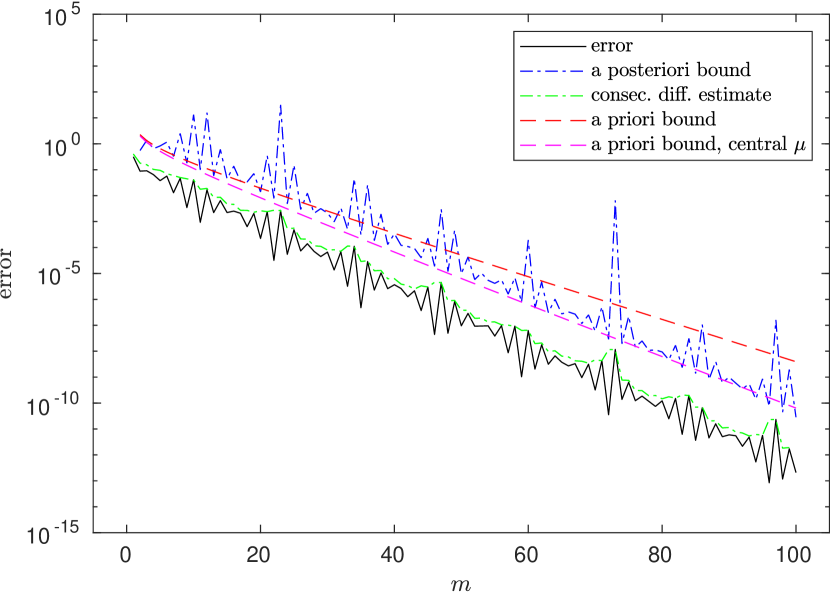
Figure 2. Approximation of $\boldsymbol{x}^{T}h_{\mu}(A)\boldsymbol{x}$ with the Lanczos algorithm, and comparison with the a priori error bound from Proposition 3.6, the a posteriori error bound from Proposition 3.8 and the consecutive difference estimate. The spectrum of $A$ has gaps in the intervals $[10,11]$ and $[20,25]$. Left: $\mu=22$. Right: $\mu=10.6$.

4. Final algorithm

In this section we put together all the theoretical results obtained in Section 3 to improve Algorithm 1 and obtain an efficient algorithm that also provides some guarantees on its output.

4.1. Choosing the input parameters

First of all, we need a criterion to decide the number $s$ of Hutchinson sample vectors and the number $m$ of Lanczos iterations. For this purpose, given a failure probability $\delta$ and a target relative gap width $\theta$, we set the goal to find all gaps in the spectrum of $A$ with relative width greater than or equal to $\theta$, with probability $1-\delta$.

How should we choose $s$ and $m$ so that all these gaps are found? Let us consider a candidate gap $[\mu_{1},\mu_{2}]\subset\mathbb{R}$ and fix a parameter $\varepsilon>0$, and say that we take $m$ such that the Lanczos approximation error for each quadratic form $\boldsymbol{x}_{i}^{T}P_{\mu}\boldsymbol{x}_{i}$ is smaller than $\varepsilon/2$ for all $\mu$ inside the gap, so that $\operatorname{tr}^{\mathrm{H}}_{s}(P_{\mu})$ is contained in an interval of width smaller than $\varepsilon$ for all $\mu\in[\mu_{1},\mu_{2}]$. Then there are two possible scenarios: either there are no eigenvalues of $A$ in the interval $[\mu_{1},\mu_{2}]$, or all the jumps in $\operatorname{tr}^{\mathrm{H}}_{s}(P_{\mu})$ associated to eigenvalues inside that interval are $\varepsilon$-small (more precisely, the sum of the heights of these jumps is smaller than $\varepsilon$). This second event has a small probability of occurring, which can be bounded using Lemma 3.2, so we can conclude that $[\mu_{1},\mu_{2}]$ is a gap in the spectrum of $A$ with high probability.

The probability that all jumps in $\operatorname{tr}^{\mathrm{H}}_{s}(P_{\mu})$ associated to eigenvalues in $[\mu_{1},\mu_{2}]$ are $\varepsilon$-small is smaller than the probability of a single jump being $\varepsilon$-small, so we can impose

$$\mathbb{P}(y_{s}\leq s\varepsilon)\leq\delta,$$

where $y_{s}$ is a $\chi^{2}$ distribution with $s$ degrees of freedom, see Section 3.2. By Lemma 3.2, this condition is satisfied provided that

$$s\geq\frac{2\log(1/\delta)}{\log(1/\varepsilon)+\varepsilon-1}.$$

If the relative width of $[\mu_{1},\mu_{2}]$ is at least $\theta$, by Proposition 3.6 we have

$$\Big{\lvert}\operatorname{tr}^{\mathrm{H}}_{s}(P_{\mu})-\frac{1}{s}\sum_{i=1}^{s}\texttt{q}_{m}^{(i)}\Big{\rvert}\leq\frac{C\sum_{i=1}^{s}\lVert\boldsymbol{x}_{i}\rVert_{2}^{2}}{s\sqrt{m-1}}\bigg{(}\frac{1-\theta}{1+\theta}\bigg{)}^{m-1},$$

where we denote by $\texttt{q}_{m}^{(i)}$ the approximation of $\boldsymbol{x}_{i}^{T}P_{\mu}\boldsymbol{x}_{i}$ after $m$ Lanczos iterations. By 3.8, the above bound is smaller than $\varepsilon/2$ if we take

(4.1) $$m\geq 1+\frac{\log\big{(}2C\sum_{i=1}^{s}\lVert\boldsymbol{x}_{i}\rVert_{2}^{2}/s\varepsilon\big{)}}{\log\big{(}(1+\theta)/(1-\theta)\big{)}},\qquad C=\frac{1-\theta}{\sqrt{\pi\theta}}+1.$$

Note that although the a priori bound in Proposition 3.6 allows us to say that the Lanczos error is smaller than $\varepsilon/2$ when $\mu$ is inside a gap wider than $\theta$, we cannot use it to determine for which values of $\mu$ this actually happens. To detect the gaps in practice, we are going to use either the a posteriori bound from Proposition 3.8 or the error estimate based on consecutive differences, and assume that it is at least as accurate as the a priori bound, i.e., that it is also smaller than $\varepsilon/2$ inside a gap with relative width $\theta$. This assumption is usually satisfied, as shown in Example 3.2, at least in the central portion of each gap.

We have obtained bounds on $s$ and $m$ that depend on $\delta$, $\theta$ and $\varepsilon$, where the latter is a parameter that can be freely chosen. In order to obtain an algorithm that is as efficient as possible, we should aim to minimize the term that dominates the computational cost of the algorithm, which is the $O(sm\,\texttt{nnz}(A))$ term corresponding to the $sm$ matrix-vector products with $A$. We have

$$sm\geq\frac{2\log(2/\delta)}{\log(1/\varepsilon)+\varepsilon-1}\cdot\bigg{(}1+\frac{\log\big{(}2C\sum_{i=1}^{s}\lVert\boldsymbol{x}_{i}\rVert_{2}^{2}/s\varepsilon\big{)}}{\log\big{(}(1+\theta)/(1-\theta)\big{)}}\bigg{)},$$

and $\varepsilon$ should be chosen in order to minimize the right hand side. With some simple computations one can show that the function

$$f(\varepsilon)=\frac{1}{\log(1/\varepsilon)+\varepsilon-1}\cdot\bigg{(}1+\frac{\log\big{(}2Cn/\varepsilon\big{)}}{\log\big{(}(1+\theta)/(1-\theta)\big{)}}\bigg{)}$$

is increasing for $\varepsilon\in(0,1)$ since $2Cn\geq 1$. Recalling that $\mathbb{E}[\lVert\boldsymbol{x}_{i}\rVert^{2}]=n$ for all $i$, this implies that we should take $\varepsilon$ as small as possible, and since $s$ must be an integer, in practice the most efficient choice is to take $\varepsilon$ so that the probability of a jump being $\varepsilon$-small is lower than $\delta$ already when $s=1$, i.e.,

(4.2) $$\varepsilon\leq e^{-1}\delta^{2}.$$

In other words, we should simply use a single quadratic form $\boldsymbol{x}^{T}P_{\mu}\boldsymbol{x}$ to estimate $\operatorname{tr}(P_{\mu})$, instead of using the more general stochastic trace estimator with $s$ different random vectors.

4.2. Detecting gaps in the spectrum

To detect the gaps in the spectrum, we use an a posteriori error bound to determine when the error of the Lanczos approximation is smaller than $\varepsilon/2$. We focus on the case $s=1$, with a single random Gaussian vector $\boldsymbol{x}\in\mathbb{R}^{n}$, since we concluded that it is the most efficient choice in Section 4.1. More precisely, for each $\mu$ we perform $m$ iterations of the Lanczos method to obtain $\texttt{q}_{m}(\mu)\approx\boldsymbol{x}^{T}P_{\mu}\boldsymbol{x}$ with the approximation 2.2, and we use either Proposition 3.8 or the estimate based on consecutive differences to obtain

$$\lvert\boldsymbol{x}^{T}P_{\mu}\boldsymbol{x}-\texttt{q}_{m}(\mu)\rvert\leq\texttt{bound}_{m}(\mu),$$

where either

$$\texttt{bound}_{m}(\mu)=\lVert\boldsymbol{x}\rVert_{2}^{2}\max_{z\in[\lambda_{\min},\lambda_{\max}]}\lvert g_{m}(z)\rvert\qquad\text{with $g_{m}(z)$ as defined in \lx@cref{creftype~refnum}{eqn:lanczos-post-bound--gm-definition}},$$

or $\texttt{bound}_{m}(\mu)=c\lvert\texttt{q}_{m}(\mu)-\texttt{q}_{m+1}(\mu)\rvert$, with a safety factor $c\geq 1$. As shown in Example 3.2, the consecutive difference error estimate is usually more accurate than the a posteriori error bound from Proposition 3.8, and very often we can also expect it to be an actual upper bound due to the oscillation in the convergence of the Lanczos algorithm. In the discussion that follows, we are going to assume that $\texttt{bound}_{m}(\mu)$ is always an upper bound for the error $\lvert\boldsymbol{x}^{T}P_{\mu}\boldsymbol{x}-\texttt{q}_{m}(\mu)\rvert$; since there is no guarantee that this is true for the consecutive difference estimate, we will discuss some ways to make it more robust in Example 4.1. For all $\mu$, letting

$$\texttt{q}^{\text{U}}_{m}(\mu) :=\texttt{q}_{m}(\mu)+\texttt{bound}_{m}(\mu),$$

$$\texttt{q}^{\text{L}}_{m}(\mu) :=\texttt{q}_{m}(\mu)-\texttt{bound}_{m}(\mu),$$

we have $\boldsymbol{x}^{T}P_{\mu}\boldsymbol{x}\in[\texttt{q}^{\text{L}}_{m}(\mu),\texttt{q}^{\text{U}}_{m}(\mu)]$.

Recalling that the quadratic form $\boldsymbol{x}^{T}P_{\mu}\boldsymbol{x}$ is an increasing function of $\mu$, we can refine the upper and lower bounds $\texttt{q}^{\text{U}}_{m}(\mu)$ and $\texttt{q}^{\text{L}}_{m}(\mu)$. Indeed, we can also take the upper and lower bounds to be increasing in $\mu$: specifically, for any $\mu<\mu^{\prime}$ we must have

$$\boldsymbol{x}^{T}P_{\mu}\boldsymbol{x}\leq\boldsymbol{x}^{T}P_{\mu^{\prime}}\boldsymbol{x}\leq\texttt{q}^{\text{U}}_{m}(\mu^{\prime})\qquad\text{and}\qquad\boldsymbol{x}^{T}P_{\mu^{\prime}}\boldsymbol{x}\geq\boldsymbol{x}^{T}P_{\mu}\boldsymbol{x}\geq\texttt{q}^{\text{L}}_{m}(\mu),$$

so we can replace the bounds $\texttt{q}^{\text{U}}_{m}(\mu)$ and $\texttt{q}^{\text{L}}_{m}(\mu)$ with, respectively,

(4.3) $$\widehat{\texttt{q}}^{\text{U}}_{m}(\mu):=\min_{\mu^{\prime}\geq\mu}\texttt{q}^{\text{U}}_{m}(\mu^{\prime})\qquad\text{and}\qquad\widehat{\texttt{q}}^{\text{L}}_{m}(\mu):=\max_{\mu^{\prime}\leq\mu}\texttt{q}^{\text{L}}_{m}(\mu^{\prime}).$$

Note that the bounds $\widehat{\texttt{q}}^{\text{U}}_{m}(\mu)$ and $\widehat{\texttt{q}}^{\text{L}}_{m}(\mu)$ are by construction increasing functions of $\mu$. We can further improve the bounds by taking the best ones over several values of $m$. Indeed, given a set of positive integers $\mathcal{M}\subset\mathbb{N}$, we can define

(4.4) $$\widehat{\texttt{q}}^{\text{U}}_{\mathcal{M}}(\mu):=\min_{m\in\mathcal{M}}\widehat{\texttt{q}}^{\text{U}}_{m}(\mu)\qquad\text{and}\qquad\widehat{\texttt{q}}^{\text{L}}_{\mathcal{M}}(\mu):=\max_{m\in\mathcal{M}}\widehat{\texttt{q}}^{\text{L}}_{m}(\mu),$$

and we still have $\boldsymbol{x}^{T}P_{\mu}\boldsymbol{x}\in[\widehat{\texttt{q}}^{\text{L}}_{\mathcal{M}}(\mu),\widehat{\texttt{q}}^{\text{U}}_{\mathcal{M}}(\mu)]$. Using a set $\mathcal{M}$ with more than a single value of $m$ can be useful to improve the bounds in the case when there is an eigenvalue of $T_{m}$ inside one of the gaps. In such a situation, by considering bounds for $\mathcal{M}=\{m-d,\dots,m-1,m\}$ there is a higher chance that one of the matrices $T_{m-j}$, $j=0,\dots,d$ has no eigenvalues in the gap, so the bounds $\widehat{\texttt{q}}^{\text{U}}_{\mathcal{M}}(\mu)$ and $\widehat{\texttt{q}}^{\text{L}}_{\mathcal{M}}(\mu)$ are likely going to be better than $\widehat{\texttt{q}}^{\text{U}}_{m}(\mu)$ and $\widehat{\texttt{q}}^{\text{L}}_{m}(\mu)$.

After incorporating these improvements, we can conclude that if $\varepsilon$ is chosen according to 4.2 and for some $\mu_{1}<\mu_{2}$ we have $\lvert\widehat{\texttt{q}}^{\text{U}}_{\mathcal{M}}(\mu_{2})-\widehat{\texttt{q}}^{\text{L}}_{\mathcal{M}}(\mu_{1})\rvert\leq\varepsilon$, then there are no eigenvalues of $A$ in the interval $[\mu_{1},\mu_{2}]$ with probability at least $1-\delta$.

4.3. Algorithm summary

The analysis in the previous sections leads to the following algorithm, whose pseudocode is given in Algorithm 2. Given an input failure probability $\delta$ and target relative gap width $\theta$, we first compute $\varepsilon$ according to 4.2 such that the probability of having an $\varepsilon$-small jump at an eigenvalue in Hutchinson’s trace estimator is less than $\delta$ when using a single random vector (i.e., with $s=1$). We then use Proposition 3.6 to select the number $m$ of Lanczos iterations that ensures that the error of the Lanczos approximation to the quadratic form $\boldsymbol{x}^{T}h_{\mu}(A)\boldsymbol{x}$ is smaller than $\varepsilon/2$ whenever $\mu$ is inside a gap with relative width at least $\theta$. As an alternative, we could fix the number of Lanczos iterations $m$ a priori, but by doing so we would lose the guarantee that all the gaps with width larger than $\theta$ are located. Then, we run $m$ iterations of the Lanczos method to compute the approximation 2.2 and the upper and lower a posteriori bounds $\widehat{\texttt{q}}^{\text{U}}_{\mathcal{M}}(\mu)$ and $\widehat{\texttt{q}}^{\text{L}}_{\mathcal{M}}(\mu)$ defined in 4.4, for all input values of $\mu$ and a set $\mathcal{M}$ of integers smaller than or equal to $m$, such as $\{m-d,\dots,m-1,m\}$, with, e.g., $d=2$. All the intervals $[\mu_{1},\mu_{2}]$ such that $\lvert\widehat{\texttt{q}}^{\text{U}}_{\mathcal{M}}(\mu_{2})-\widehat{\texttt{q}}^{\text{L}}_{\mathcal{M}}(\mu_{1})\rvert\leq\varepsilon$ are hence gaps in the spectrum of $A$ with probability at least $1-\delta$.

Algorithm 2 Eigenvalue gap finder

1:Symmetric matrix $A\in\mathbb{R}^{n\times n}$, failure probability $\delta$, target relative gap size $\theta$, vector of test parameters $\boldsymbol{\mu}=[\mu_{1},\dots,\mu_{N_{f}}]$

2:$\texttt{tr}_{j}\approx\operatorname{tr}(P_{\mu_{j}})$ for $j=1,\dots,N_{f}$, intervals $[a_{i},b_{i}]$ that contain no eigenvalues of $A$ with probability $1-\delta$ each

3:Compute $\varepsilon$ according to 4.2, ensuring that the probability of a jump being smaller than $\varepsilon$ with $s=1$ Hutchinson vectors is smaller than $\delta$.

4:Draw a random Gaussian vector $\boldsymbol{x}\in\mathbb{R}^{n}$.

5:Compute $m$ according to 4.1, ensuring that the Lanczos approximation 2.2 to $\boldsymbol{x}^{T}P_{\mu}\boldsymbol{x}$ has an error smaller than $\varepsilon/2$ if $\mu$ is within a gap of relative width $\theta$ or larger.

6:Select a set $\mathcal{M}$ of integers smaller than or equal to $m$, such as $\mathcal{M}=\{m-4,\dots,m-1,m\}$.

7:Compute $V_{m}$ and $\underline{T}_{m}$ by running $m$ iterations of the Lanczos algorithm with the matrix $A$ and the vector $\boldsymbol{x}$.

8:Compute the eigendecomposition $T_{m}=U_{m}^{T}D_{m}U_{m}$ and $\boldsymbol{w}_{m}=\lVert\boldsymbol{x}\rVert_{2}U_{m}\boldsymbol{e}_{1}$.

9:for $j=1,\dots,N_{f}$ do

10:     Compute $\texttt{q}_{m,j}=\boldsymbol{w}_{m}^{T}h_{\mu_{j}}(D_{m})\boldsymbol{w}_{m}$.

11:     for $m^{\prime}\in\mathcal{M}$ do

12:          Compute the monotone upper and lower bounds $\widehat{\texttt{q}}^{\text{U}}_{m^{\prime}}(\mu_{j})$ and $\widehat{\texttt{q}}^{\text{L}}_{m^{\prime}}(\mu_{j})$ using 4.3, where $\texttt{bound}_{m^{\prime}}(\mu_{j})$ is obtained either with Proposition 3.8 or by running Lanczos for one additional iteration to compute $\lvert\texttt{q}_{m^{\prime},j}-\texttt{q}_{m^{\prime}+1,j}\rvert$.

13:     end for

14:     Compute the bounds $\widehat{\texttt{q}}^{\text{U}}_{\mathcal{M}}(\mu_{j})=\displaystyle\min_{m^{\prime}\in\mathcal{M}}\widehat{\texttt{q}}^{\text{U}}_{m^{\prime}}(\mu_{j})$ and $\widehat{\texttt{q}}^{\text{L}}_{\mathcal{M}}(\mu_{j})=\displaystyle\max_{m^{\prime}\in\mathcal{M}}\widehat{\texttt{q}}^{\text{L}}_{m^{\prime}}(\mu_{j})$.

15:end for

16:Compute $\widehat{\texttt{q}}^{\text{U}}_{\mathcal{M}}(\boldsymbol{\mu})-\widehat{\texttt{q}}^{\text{L}}_{\mathcal{M}}(\boldsymbol{\mu})$ and determine the largest intervals $[a_{i},b_{i}]$ such that $\lvert\widehat{\texttt{q}}^{\text{U}}_{\mathcal{M}}(b_{i})-\widehat{\texttt{q}}^{\text{L}}_{\mathcal{M}}(a_{i})\rvert\leq\varepsilon$.

Note that $m$ is selected so that the a priori error bound on the approximation of $\boldsymbol{x}^{T}h_{\mu}(A)\boldsymbol{x}$ from Proposition 3.6 is smaller than $\varepsilon/2$ whenever $\mu$ is inside a gap with relative width at least $\theta$, so, assuming that the a posteriori error bound or estimate is at least as accurate as the a priori one, we expect that all gaps of relative width $\theta$ or larger are detected by Algorithm 2. Numerical evidence shows that this assumption is generally satisfied when $\mu$ is not too close to the extrema of the gap and $\varepsilon$ is not too large. We also mention that, although Algorithm 2 cannot explicitly find the gap between the $k$-th and the $(k+1)$-th eigenvalue for a given $k$, it still computes estimates for $\operatorname{tr}(P_{\mu_{j}})$ for all $\mu_{j}\in\boldsymbol{\mu}$, so we know the approximate number of eigenvalues below each detected gap and thus we can roughly determine if one of the gaps found by the algorithm is likely to be the one between $\lambda_{k}$ and $\lambda_{k+1}$ (of course, we can only expect that Algorithm 2 will detect this gap if we assume that it is wide enough). If more accuracy on the number of eigenvalues below each gap is required, then one should use a larger number $s$ of sample vectors for Hutchinson’s trace estimator. Alternatively, if it is feasible to compute an $LDL^{T}$ factorization, it can be used to compute the exact number of eigenvalues below a certain gap in order to verify if it corresponds to the searched gap between the eigenvalues $\lambda_{k}$ and $\lambda_{k+1}$.

Remark 4.1.

Recall that $\boldsymbol{x}^{T}P_{\mu}\boldsymbol{x}$ is a staircase-like piecewise constant function of $\mu$, and in particular it must be constant in any interval that contains no eigenvalues of $A$. This means that given a candidate gap $[\mu_{1},\mu_{2}]$, in addition to the condition $\lvert\widehat{\texttt{q}}^{\text{U}}_{\mathcal{M}}(\mu_{2})-\widehat{\texttt{q}}^{\text{L}}_{\mathcal{M}}(\mu_{1})\rvert\leq\varepsilon$, we also need to check that $\widehat{\texttt{q}}^{\text{L}}_{\mathcal{M}}(\mu_{2})<\widehat{\texttt{q}}^{\text{U}}_{\mathcal{M}}(\mu_{1})$. If this additional condition is not satisfied, it is impossible for $\boldsymbol{x}^{T}P_{\mu}\boldsymbol{x}$ to be a constant function for $\mu\in[\mu_{1},\mu_{2}]$, and hence we can conclude with certainty that there must be at least one eigenvalue of $A$ in the interval $[\mu_{1},\mu_{2}]$. This seems to cause a contradiction when the condition $\lvert\widehat{\texttt{q}}^{\text{U}}_{\mathcal{M}}(\mu_{2})-\widehat{\texttt{q}}^{\text{L}}_{\mathcal{M}}(\mu_{1})\rvert\leq\varepsilon$ is verified but $\widehat{\texttt{q}}^{\text{L}}_{\mathcal{M}}(\mu_{2})<\widehat{\texttt{q}}^{\text{U}}_{\mathcal{M}}(\mu_{1})$ is not, since it would imply that all the eigenvalues of $A$ contained in $[\mu_{1},\mu_{2}]$ have an associated $\varepsilon$-small jump, which is a low-probability event. However, it simply means that this situation is very unlikely to happen in a practical scenario, and it would probably not be encountered if the algorithm is run on the same problem for a second time.

4.4. Computational cost

The most expensive operations in Algorithm 2 are the $m$ matrix-vector products with $A$ required to construct the Krylov basis in the Lanczos algorithm, which cost $O(m\,\texttt{nnz}(A))$ for a sparse matrix $A$. The additional operations done for the computation of the quadratic forms $\boldsymbol{x}^{T}P_{\mu_{j}}\boldsymbol{x}$ with $N_{f}$ different parameters $\mu_{j}$ add up to $O(nm+m^{3}+mN_{f})$, as discussed in Section 2.3. If we estimate the error with the consecutive difference estimate, we have to run the Lanczos algorithm for one additional iteration, and compute the differences $\lvert\texttt{q}_{m^{\prime},j}-\texttt{q}_{m^{\prime}+1,j}\rvert$ for all $m^{\prime}\in\mathcal{M}$. If $\lvert\mathcal{M}\rvert=d$ and the elements of $\mathcal{M}$ are consecutive integers, this amounts to computing $d+1$ quadratic forms $\texttt{q}_{m^{\prime},j}$ for all $j$, so the additional cost is $O(m^{3}d+mN_{f}d)$.

On the other hand, if we use the a posteriori error bound from Proposition 3.8, we have to evaluate the coefficients $\alpha_{j}$, $\beta_{j}$ and $\gamma_{j}$ for all $\mu_{j}$, which can be done with $O(m^{2})$ operations assuming that the eigenvalue decomposition of $T_{m}$ is available, and compute the maximum of $\lvert g_{m}(z)\rvert$ over $[\lambda_{\min},\lambda_{\max}]$, where $g_{m}$ is defined in 3.10. The evaluation of $g_{m}(z)$ for all $\mu_{j}$ at a single point $z$ requires $O(mN_{f})$ operations, and if a discretization of $[\lambda_{\min},\lambda_{\max}]$ with $L$ points is used, we can approximately evaluate the bound in Proposition 3.8 for all $\mu_{j}$ with $O(m^{2}+mN_{f}L)$ operations. If a set $\mathcal{M}$ with $d$ elements is used to compute the more robust bounds $\widehat{\texttt{q}}^{\text{U}}_{\mathcal{M}}(\mu_{j})$ and $\widehat{\texttt{q}}^{\text{L}}_{\mathcal{M}}(\mu_{j})$, the cost for the computation of the bounds is roughly multiplied by a factor $d$ and becomes $O(m^{3}d+mN_{f}Ld)$, where we have also included the cost of computing the eigenvalues and eigenvectors of $T_{m^{\prime}}$ for $m^{\prime}\in\mathcal{M}$. Note that given $\texttt{q}^{\text{U}}_{m}(\mu_{j})$ and $\texttt{q}^{\text{L}}_{m}(\mu_{j})$, the refined bounds $\widehat{\texttt{q}}^{\text{U}}_{m}(\mu_{j})$ and $\widehat{\texttt{q}}^{\text{L}}_{m}(\mu_{j})$ described in Section 4.2 can be computed for all $\mu_{j}$ with $O(N_{f})$ operations. Finally, once $\widehat{\texttt{q}}^{\text{U}}_{\mathcal{M}}(\mu_{j})$ and $\widehat{\texttt{q}}^{\text{L}}_{\mathcal{M}}(\mu_{j})$ have been computed, the gaps can be located with a cost of $O(N_{f})$. The total computational cost of Algorithm 2 is therefore $O(m\,\texttt{nnz}(A)+nm+m^{3}d+mN_{f}d)$ with the consecutive difference estimate, and $O(m\,\texttt{nnz}(A)+nm+m^{3}d+mN_{f}Ld)$ with the a posteriori bound from Proposition 3.8.

Note that all operations associated with different values of $\mu$ are completely independent, so the algorithm can be easily parallelized, for instance by assigning different slices of the spectral interval to different processors. This parallelization is not particularly helpful when the matrix size $n$ is large enough, since the dominant part of the computation would still be the $O(m\,\texttt{nnz}(A))$ term associated with matrix-vector products with $A$; however, parallelizing the computations associated with different parameters $\mu$ can be helpful for mitigating the $O(mN_{f}Ld)$ cost of computing the a posteriori error bounds from Proposition 3.8, which can become quite high if both $N_{f}$ and $L$ are large, see, for instance, the experiment in Section 5.3.

If our goal is to detect all gaps with relative width larger than $\theta$ with probability at least $1-\delta$, we should take $m$ according to 4.1 with $\varepsilon\leq e^{-1}\delta^{2}$, i.e.,

(4.5) $$m\geq 1+\frac{1+\log\big{(}2C\lVert\boldsymbol{x}\rVert_{2}^{2}/\delta^{2}\big{)}}{\log\big{(}(1+\theta)/(1-\theta)\big{)}},\qquad C=\frac{1-\theta}{\sqrt{\pi\theta}}+1,$$

where we recall that $\mathbb{E}[\lVert\boldsymbol{x}\rVert_{2}^{2}]=n$. By looking at the behavior of the right-hand side of 4.5 as $\theta\to 0$, using the fact that

$$\log\bigg{(}\frac{1+\theta}{1-\theta}\bigg{)}\approx\frac{1}{2\theta},$$

we conclude that for small $\theta$ we should take

$$m\approx\log\bigg{(}\frac{2\lVert\boldsymbol{x}\rVert_{2}^{2}}{\delta^{2}\sqrt{\pi\theta}}\bigg{)}\frac{1}{2\theta}.$$

Although the dependence of $m$ on the failure probability $\delta$ and the matrix size $n$ is not particularly severe since they appear inside a logarithm, the main drawback of this approach is the $O(1/\theta)$ dependence on the relative gap width $\theta$, which causes Algorithm 2 to quickly become more expensive as the target gap width is reduced. This is an inherent limitation of the Lanczos method for the computation of $\boldsymbol{x}^{T}P_{\mu}\boldsymbol{x}$, and more precisely of the polynomial approximation of the sign function (see Proposition 3.3). As we mentioned in Section 3.3, Proposition 3.3 can be improved by considering two nonsymmetric intervals as in [10], and this would in turn lead to an improved estimate on the required number of Lanczos iterations $m$; however, in general we do not expect to find an asymptotic estimate that is better than $m=O(1/\theta)$. Indeed, for a gap located near the center of $\operatorname{\Lambda}(A)$, the spectrum of $A$ is contained in two intervals that are approximately symmetric with respect to the gap, and there would not be any significant advantage in using the improved result [10, Theorem 1.1].

Example 4.1.

In this example we show how the bounds described in Section 4.2 perform on the simple test problem from Example 3.1. The matrix $A$ is $600\times 600$, with $\operatorname{\Lambda}(A)\subset[0,60]$ and three gaps in the spectrum given by the intervals $[20,21]$, $[30,32]$ and $[40,44]$. We use a single Gaussian vector $\boldsymbol{x}\in\mathbb{R}^{n}$ for Hutchinson’s estimator and $m=50$ Lanczos iterations. We compare the exact $\boldsymbol{x}^{T}P_{\mu}\boldsymbol{x}$ with the upper and lower bounds $\widehat{\texttt{q}}^{\text{U}}_{\mathcal{M}}(\mu)$ and $\widehat{\texttt{q}}^{\text{L}}_{\mathcal{M}}(\mu)$ obtained both with Proposition 3.8 and with the consecutive difference error estimate. In particular, for the latter we use the error estimate $\texttt{bound}_{m}(\mu_{j})=c\lvert\texttt{q}_{m,j}-\texttt{q}_{m+1,j}\rvert$, with a safety factor $c=2$. In both cases, we take $\mathcal{M}=\{m-d+1,\dots,m\}$ with $d=3$. Since $c\lvert\texttt{q}_{m,j}-\texttt{q}_{m+1,j}\rvert$ is not guaranteed to be an upper bound for $\lvert\boldsymbol{x}^{T}P_{\mu_{j}}\boldsymbol{x}\rvert$, the inequalities $\widehat{\texttt{q}}^{\text{L}}_{\mathcal{M}}(\mu)\leq\boldsymbol{x}^{T}P_{\mu}\boldsymbol{x}\leq\widehat{\texttt{q}}^{\text{U}}_{\mathcal{M}}(\mu)$ do not necessarily hold for all $\mu$, especially after the two minimizations and maximizations in 4.3 and 4.4. To overcome this issue, we also propose to use a “safe” variant of the upper and lower estimates for $\boldsymbol{x}^{T}P_{\mu}\boldsymbol{x}$, defined as

(4.6) $$\widehat{\texttt{q}}^{\mathrm{U}\star}_{\mathcal{M}}(\mu):=\max_{m\in\mathcal{M}}\widehat{\texttt{q}}^{\text{U}}_{m}(\mu)\qquad\text{and}\qquad\widehat{\texttt{q}}^{\mathrm{L}\star}_{\mathcal{M}}(\mu):=\min_{m\in\mathcal{M}}\widehat{\texttt{q}}^{\text{L}}_{m}(\mu),$$

which correspond to taking the worst of the bounds associated with $\mathcal{M}$ instead of the best ones. This variant significantly increases the chance that $\widehat{\texttt{q}}^{\mathrm{U}\star}_{\mathcal{M}}(\mu)$ and $\widehat{\texttt{q}}^{\mathrm{L}\star}_{\mathcal{M}}(\mu)$ are an upper and lower bound for $\boldsymbol{x}^{T}P_{\mu}\boldsymbol{x}$, respectively, although it reduces the overall accuracy of the estimates.

The bounds are shown in Figure 3, including the safe variants $\widehat{\texttt{q}}^{\mathrm{U}\star}_{\mathcal{M}}(\mu)$ and $\widehat{\texttt{q}}^{\mathrm{L}\star}_{\mathcal{M}}(\mu)$ of the bounds obtained by using consecutive differences. Notice that the upper and lower estimates $\widehat{\texttt{q}}^{\text{U}}_{\mathcal{M}}(\mu)$ and $\widehat{\texttt{q}}^{\text{L}}_{\mathcal{M}}(\mu)$ computed with consecutive differences are much closer to $\boldsymbol{x}^{T}P_{\mu}\boldsymbol{x}$ compared to the bounds obtained with Proposition 3.8, but they sometimes fail to satisfy $\widehat{\texttt{q}}^{\text{L}}_{\mathcal{M}}(\mu)\leq\boldsymbol{x}^{T}P_{\mu}\boldsymbol{x}\leq\widehat{\texttt{q}}^{\text{U}}_{\mathcal{M}}(\mu)$: see for instance the right plot in Figure 3, which is a close-up of the larger gap $[40,44]$. On the other hand, the safe variants $\widehat{\texttt{q}}^{\mathrm{U}\star}_{\mathcal{M}}(\mu)$ and $\widehat{\texttt{q}}^{\mathrm{L}\star}_{\mathcal{M}}(\mu)$ are more robust, while still being more accurate than the a posteriori bounds from Proposition 3.8. To provide a quantitative comparison, for the plot in Figure 3 we used $4000$ different shift parameters $\mu_{j}$, and the inequality $\boldsymbol{x}^{T}P_{\mu_{j}}\boldsymbol{x}\leq\widehat{\texttt{q}}^{\text{U}}_{\mathcal{M}}(\mu_{j})$ was not satisfied for $251$ of them, while $\boldsymbol{x}^{T}P_{\mu_{j}}\boldsymbol{x}\leq\widehat{\texttt{q}}^{\mathrm{U}\star}_{\mathcal{M}}(\mu_{j})$ was not satisfied for only $35$ values of $j$. Note that the fraction of values of $\mu$ for which the safe upper estimate $\widehat{\texttt{q}}^{\mathrm{U}\star}_{\mathcal{M}}(\mu)$ fails to be an upper bound is smaller than $10^{-2}$, which is the failure probability that we use for the experiments in Section 5.

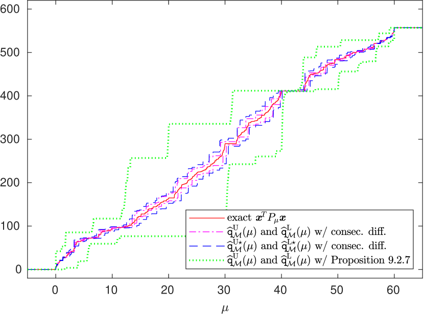
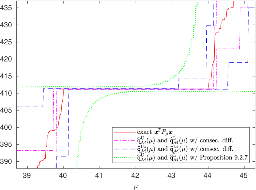
Figure 3. Upper and lower bounds for $\boldsymbol{x}^{T}P_{\mu}\boldsymbol{x}$ obtained with the Lanczos algorithm with $m=50$ iterations. The right plot is a close-up of the left plot around the larger gap $[40,44]$.

5. Numerical experiments

In this section we run some experiments to investigate the performance of Algorithm 2. For all the experiments, we use Algorithm 2 with a failure probability $\delta=10^{-2}$ and a number of Lanczos iterations $m$ that is either fixed in advance or computed according to 4.5 in order to find all gaps with relative width larger than a certain target $\theta$. When not stated differently, for the Lanczos algorithm we employ the error estimate $\texttt{bound}_{m}(\mu_{j})=c\lvert\texttt{q}_{m,j}-\texttt{q}_{m,j+1}\rvert$ with a safety factor $c=2$, and we use the more robust upper and lower estimates $\widehat{\texttt{q}}^{\mathrm{U}\star}(\mu)$ and $\widehat{\texttt{q}}^{\mathrm{L}\star}(\mu)$ defined in 4.6, with $\mathcal{M}=\{m-d+1,\dots,m\}$ with $d=3$. These estimates are cheaper to compute compared to the a posteriori error bound from Proposition 3.8, and they are also quite reliable, as shown in Example 4.1. Even though the estimate $c\lvert\texttt{q}_{j,m}-\texttt{q}_{j,m+1}\rvert$ does not have the same theoretical guarantees as the a posteriori error bound, we have seen in Example 3.2 that it is usually much closer to the actual error. All the experiments have been done using MATLAB R2021b on a laptop running Ubuntu 20.04, with 32 GB of RAM and an Intel Core i5-10300H CPU with clock rate 2.5 GHz. The code to reproduce the experiments in this section is available on Github at https://github.com/simunec/eigenvalue-gap-finder.

5.1. Scaling with the gap width

We start by examining the behavior of Algorithm 2 with respect to the relative gap width $\theta$. We consider a symmetric tridiagonal matrix $A$ of size $n=30000$ obtained as a sum $A=D+T$, where $T$ is a random symmetric tridiagonal matrix with $\mathcal{N}(0,1)$ entries and $D$ is a diagonal matrix. The eigenvalues of $D$ are chosen so that the spectrum of $A$ has a gap with relative width approximately $\theta$. Specifically, the eigenvalues of $D$ are contained in the intervals $[1,10^{3}]\cup[10^{3}+x,10^{4}]$, where $x$ satisfies

$$\frac{x/2}{10^{4}-10^{3}-x/2}=\theta,$$

so that the relative width of the gap $[10^{3},10^{3}+x]$ is $\theta$, and hence the spectrum of the perturbed matrix $A=D+T$ also has a gap with relative width approximately $\theta$. We consider a matrix $D$ with $20000$ logspaced eigenvalues in $[1,10^{3}]$ and $10000$ logspaced eigenvalues in $[10^{3}+x,10^{4}]$.

We estimate this gap using Algorithm 2, with $m$ computed according to 4.5, so that we can expect it to successfully find all gaps with relative width larger than $\theta$; we use $N_{f}=10000$ parameters $\mu$, logarithmically spaced on the interval $[1,10^{4}]$. For each $\theta$, in Table 1 we show the true gap computed by diagonalizing $A$, the gap estimated by Algorithm 2 and the approximate number of eigenvalues below the gap, obtained by rounding the trace approximation $\boldsymbol{x}^{T}P_{\mu}\boldsymbol{x}$ for $\mu$ equal to the left endpoint of the estimated gap, as well as the number of Lanczos iterations $m$, the execution time of the algorithm and the time required for the computation of the eigenvalues of $A$. We see that the gap is found successfully for all $\theta$, with the estimated gap being slightly larger than the true gap only for $\theta=0.1$ and $\theta=0.05$. The estimated number of eigenvalues below the gap roughly approximates the exact value $20000$, but it is still relatively far from the correct number since we are using only one sample vector for Hutchinson’s estimator. Note that the number of Lanczos iterations scales approximately as $O(1/\theta)$, but the execution time increases more than linearly in the number of Lanczos iterations $m$; this is likely due to the $O(m^{3})$ cost for the computation of eigenvalues and eigenvectors of the projected matrix $T_{m}$ becoming the dominant part of the computation when the subspace dimension $m$ is large. On the other hand, the execution time for eig remains constant, so when the gap width $\theta$ becomes sufficiently small it would be more efficient to directly diagonalize the matrix instead of using Algorithm 2. Of course, this would not be the case if the matrix dimension $n$ increases, as we show in the following experiment.

Table 1. Performance of Algorithm 2 with $n=30000$ and varying gap width $\theta$.

$\theta$	true gap	estim. gap	estim. $\operatorname{n_{e}}(\mu)$	Lanczos its.	time (s)	time eig (s)
$0.1$	$[$1001.80, 2633.87$]$	$[$1016.48, 2637.19$]$	$19\,637$	$112$	0.114	2.985
$0.05$	$[$1001.65, 1856.42$]$	$[$999.77, 1856.64$]$	$19\,776$	$226$	0.209	2.798
$0.025$	$[$1001.15, 1435.81$]$	$[$1001.61, 1434.55$]$	$20\,198$	$456$	0.359	2.907
$0.01$	$[$1001.17, 1175.30$]$	$[$1001.61, 1174.65$]$	$20\,027$	$1156$	1.025	2.645
$0.005$	$[$1000.69, 1085.83$]$	$[$1000.69, 1085.18$]$	$19\,862$	$2342$	2.451	2.909
$0.0025$	$[$1003.69, 1042.75$]$	$[$1004.38, 1042.08$]$	$19\,709$	$4745$	7.160	2.924

5.2. Scaling with the matrix size

Let us now consider a sequence of matrices with increasing size and approximately constant gap width. We use a setup similar to Section 5.2, with fixed relative gap width $\theta=0.01$ and increasing matrix size $n$. We take $A=D+T$, where $T$ is symmetric tridiagonal with random $\mathcal{N}(0,1)$ entries and $D$ is diagonal with $\operatorname{\Lambda}(A)\subset[1,10^{3}]\cup[10^{3}+x,10^{4}]$, with $n/2$ logspaced eigenvalues below the gap and $n/2$ logspaced eigenvalues above the gap. The value of $x$ is chosen so that $A$ has relative gap width approximately $\theta$, as in Section 5.2.

We use Algorithm 2 to estimate the gap, with the number of Lanczos iterations $m$ computed according to 4.5 and $N_{f}=10000$ parameters $\mu$, logarithmically spaced over the interval $[1,10^{4}]$. The results for a matrix dimension that increases from $n=5000$ to $n=80000$ are shown in Table 2. In this case, the gap is found correctly for all matrix sizes, with none of the estimated gaps being larger than the true gap computed via a diagonalization. Note that the number of Lanczos iterations increases very slowly with the matrix dimension, in accordance with the discussion in Section 4.4. Hence, the execution time of the algorithm increases roughly linearly, since with a large matrix size $n$ and moderate subspace dimension $m$ the leading term in the computational cost is given by the $m$ matrix-vector products with $A$ in the construction of the Lanczos basis, which cost $O(mn)$ for a tridiagonal matrix. On the other hand, the time required for computing the eigenvalues of the tridiagonal matrix $A$ scales like $O(n^{2})$, so it quickly becomes more expensive than Algorithm 2. Note that if $A$ was a sparse matrix that is not tridiagonal, the diagonalization time would scale like $O(n^{3})$, making the difference between the two approaches even more evident.

Table 2. Performance of Algorithm 2 with fixed gap width $\theta=0.01$ and increasing matrix size $n$.

$n$	true gap	estim. gap	estim. $\operatorname{n_{e}}(\mu)$	Lanczos its.	time (s)	time eig (s)
$5000$	$[$1000.58, 1177.15$]$	$[$1000.69, 1176.81$]$	$2377$	$1067$	0.412	$0.115$
$10\,000$	$[$1001.11, 1175.88$]$	$[$1001.61, 1175.73$]$	$4956$	$1101$	0.548	$0.378$
$20\,000$	$[$1000.23, 1177.01$]$	$[$1000.69, 1176.81$]$	$9835$	$1136$	0.806	$1.355$
$40\,000$	$[$1002.67, 1175.70$]$	$[$1003.46, 1174.65$]$	$19\,930$	$1171$	1.236	$4.760$
$80\,000$	$[$1001.39, 1176.18$]$	$[$1001.61, 1175.73$]$	$39\,874$	$1205$	2.237	$16.337$

It is interesting to observe that Algorithm 2 can be also used to cheaply obtain a rough estimate of the gap by taking a larger failure probability $\delta$ and fixing the number of Lanczos iterations $m$ in advance instead of computing it with 4.5. For instance, we show in Table 3 the performance of Algorithm 2 with $\delta=0.5$ and $m=250$. We see that the gap in the spectrum is still located successfully, although the accuracy is generally lower and sometimes the estimated gap is larger than the true gap, for instance in the case $n=5000$. Note that the estimated number of eigenvalues below the gap coincides with the corresponding number from Table 2, even if the number of Lanczos iterations is different: this happens because we used the same random vector $\boldsymbol{x}$ for Hutchinson’s trace estimator, and in both cases we are approximating the same quadratic form $\boldsymbol{x}^{T}P_{\mu}\boldsymbol{x}$ (the values of $\mu$ in the two cases may be different, but as long as they are both inside the gap the corresponding values of $\boldsymbol{x}^{T}P_{\mu}\boldsymbol{x}$ coincide). In particular, this also confirms that the error in the estimated number of eigenvalues below the gap is essentially only due to the error in the stochastic trace estimator, and not to the error in the approximation of the quadratic form via the Lanczos algorithm.

Table 3. Performance of Algorithm 2 with fixed gap width $\theta=0.01$ and increasing matrix size $n$. The number of Lanczos iterations is fixed to $m=250$ and the failure probability is set to $\delta=0.5$.

$n$	true gap	estim. gap	estim. $\operatorname{n_{e}}(\mu)$	Lanczos its.	time (s)	time eig (s)
$5000$	$[$1000.58, 1177.15$]$	$[$998.85, 1178.98$]$	$2377$	$250$	0.102	$0.114$
$10\,000$	$[$1001.11, 1175.88$]$	$[$1003.46, 1170.33$]$	$4956$	$250$	0.123	$0.386$
$20\,000$	$[$1000.23, 1177.01$]$	$[$1001.61, 1167.10$]$	$9835$	$250$	0.188	$1.353$
$40\,000$	$[$1002.67, 1175.70$]$	$[$1002.54, 1161.73$]$	$19\,930$	$250$	0.281	$4.757$
$80\,000$	$[$1001.39, 1176.18$]$	$[$1005.31, 1175.73$]$	$39\,874$	$250$	0.467	$16.454$

5.3. A real-world example

We conclude the experiments with an example using a matrix from the SuiteSparse Matrix Collection [6]. We take as $A$ the symmetric matrix GHS_indef/linverse, which has size $n=11999$ with $95977$ nonzero entries. The spectrum of this matrix, shown in Figure 4, has three relatively large gaps, which we aim to locate using Algorithm 2. In this test we compare the robust consecutive difference estimates defined in 4.6 with the a posteriori bound from Proposition 3.8, both obtained using $m=100$ Lanczos iterations and $d=3$. We plot in Figure 5 the approximations to $\boldsymbol{x}^{T}P_{\mu}\boldsymbol{x}$ and the upper and lower bounds obtained with the two approaches, where $\boldsymbol{x}$ is the single random vector used in Hutchinson’s estimator; we use the same vector $\boldsymbol{x}$ for the two variants of Algorithm 2. Note that the upper and lower bounds obtained by using Proposition 3.8 are much more conservative compared to those based on consecutive difference estimates, especially far from the gaps in the spectrum.

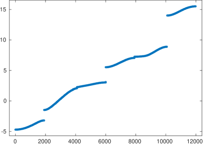
Figure 4. Spectrum of the matrix GHS_indef/linverse, with three evident gaps.

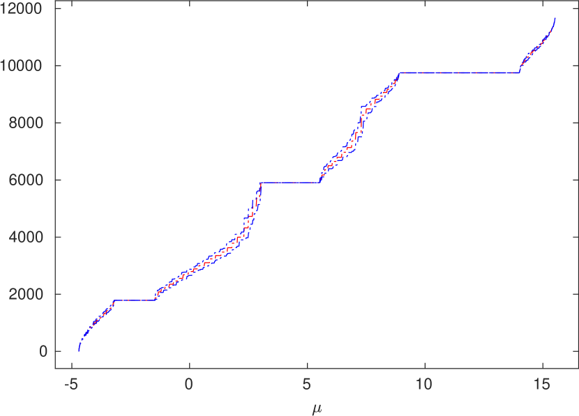
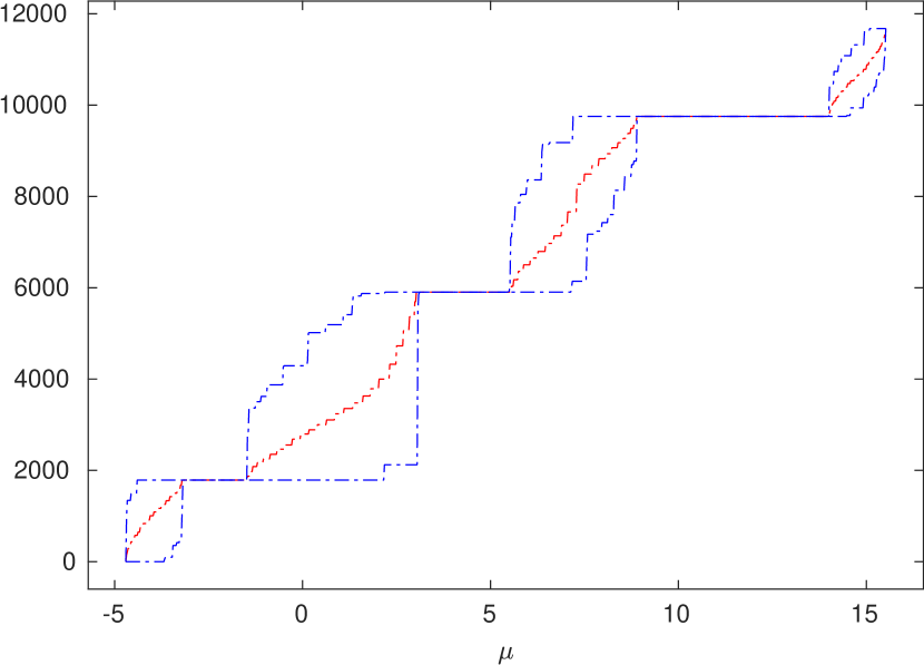
Figure 5. Approximations to $\boldsymbol{x}^{T}P_{\mu}\boldsymbol{x}$, and upper and lower bounds obtained with Algorithm 2, for several different $\mu$, with $m=250$ Lanczos iterations. Left: Algorithm 2 with robust consecutive difference error estimate 4.6. Right: Algorithm 2 with a posteriori error bound from Proposition 3.8.

Table 4. Performance of Algorithm 2 on the test matrix GHS_indef/linverse, using the robust consecutive difference estimate 4.6 and the a posteriori bound from Proposition 3.8. The number of Lanczos iterations is set to $m=100$ and the failure probability to $\delta=10^{-2}$.

method	first gap	second gap	third gap	time (s)
eig	$[$-3.201, -1.482$]$	$[$3.112, 5.531$]$	$[$8.886, 14.007$]$	$18.826$
Algorithm 2 w/ consec. diff.	$[$-3.185, -1.485$]$	$[$3.352, 5.518$]$	$[$8.979, 13.999$]$	$0.030$
Algorithm 2 w/ Proposition 3.8	$[$-2.963, -1.748$]$	$[$3.474, 5.154$]$	$[$8.999, 13.918$]$	$0.375$

The gaps found by the two variants of Algorithm 2 and the exact gaps obtained by diagonalizing $A$ are shown in Table 4, where we also include the execution times for all the methods. The gaps found by using the a posteriori bounds from Proposition 3.8 are significantly smaller than the ones obtained by estimating the Lanczos error with consecutive differences, especially for the two smaller gaps; this is a consequence of the lower accuracy of the a posteriori bounds. Moreover, the execution time is quite higher with the a posteriori bounds, due to the $O(mN_{f}Ld)$ term in the computation of the error bounds from Proposition 3.8; indeed, it turns out that this is the most expensive part of the computation in this setting, where we use $N_{f}=1000$ different values of $\mu$ and a discretization with $L=1000$ points to evaluate the maximum of $\lvert g_{m}(z)\rvert$ over the spectral interval of $A$. On the other hand, when the error in the Lanczos algorithm is estimated using consecutive differences, the portion of the computational cost that depends on $N_{f}$ scales as $O(mN_{f}d)$, which is significantly less expensive when $L=1000$ (see Section 4.4).

6. Conclusions

We have described and analyzed an algorithm for identifying gaps in the spectrum of a real symmetric matrix by simultaneously approximating the traces of spectral projectors associated with different slices of its spectrum, combining Hutchinson’s stochastic trace estimator and the Lanczos algorithm. We have investigated the behavior of Hutchinson’s estimator, and provided a priori and a posteriori error bounds for the Lanczos algorithm. This analysis has lead to an algorithm capable of detecting all gaps larger than a specified threshold with high probability. We have also determined that for this problem the best strategy is to use a single random sample vector for Hutchinson’s estimator, and utilize all the available matrix-vector products to approximate a single quadratic form via the Lanczos algorithm. Our numerical tests demonstrate that the developed algorithm can efficiently and reliably detect gaps, especially when their width is relatively large. Within our algorithm we have proposed to use either an a posteriori error bound for the Lanczos approximation error (Proposition 3.8), or a simple error estimate based on consecutive differences. Although the a posteriori error bound has better theoretical guarantees, the robust version of the error estimate from Example 4.1 has more accurate results in practice, and it is also computationally cheaper, notably when a large number of values of $\mu$ is used. Even when the algorithm fails to detect a gap, it still provides upper and lower bounds for $\boldsymbol{x}^{T}P_{\mu}\boldsymbol{x}$ for all considered values of $\mu$, which can be valuable for selecting a starting point for other algorithms, such as those based on $LDL^{T}$ factorizations.

References

- [1] M. Benzi, P. Boito, and N. Razouk, Decay properties of spectral projectors with applications to electronic structure, SIAM Rev., 55 (2013), pp. 3–64.
- [2] M. Benzi, M. Rinelli, and I. Simunec, Computation of the von Neumann entropy of large matrices via trace estimators and rational Krylov methods, Numer. Math., 155 (2023), pp. 377–414.
- [3] Å. Björck, Numerical Methods in Matrix Computations, vol. 59 of Texts in Applied Mathematics, Springer, Cham, 2015.
- [4] T. Chen, A. Greenbaum, C. Musco, and C. Musco, Error bounds for Lanczos-based matrix function approximation, SIAM J. Matrix Anal. Appl., 43 (2022), pp. 787–811.
- [5] A. Cortinovis and D. Kressner, On randomized trace estimates for indefinite matrices with an application to determinants, Found. Comput. Math., 22 (2022), pp. 875–903.
- [6] T. A. Davis and Y. Hu, The University of Florida sparse matrix collection, ACM Trans. Math. Software, 38 (2011), pp. 1–25.
- [7] E. Di Napoli, E. Polizzi, and Y. Saad, Efficient estimation of eigenvalue counts in an interval, Numer. Linear Algebra Appl., 23 (2016), pp. 674–692.
- [8] E. N. Epperly, J. A. Tropp, and R. J. Webber, XTrace: making the most of every sample in stochastic trace estimation, SIAM J. Matrix Anal. Appl., 45 (2024), pp. 1–23.
- [9] A. Eremenko and P. Yuditskii, Uniform approximation of by polynomials and entire functions, J. Anal. Math., 101 (2007), pp. 313–324.
- [10] , Polynomials of the best uniform approximation to on two intervals, J. Anal. Math., 114 (2011), pp. 285–315.
- [11] A. Frommer and P. Maass, Fast CG-based methods for Tikhonov-Phillips regularization, SIAM J. Sci. Comput., 20 (1999), pp. 1831–1850.
- [12] A. Frommer, M. Rinelli, and M. Schweitzer, Analysis of stochastic probing methods for estimating the trace of functions of sparse symmetric matrices, Math. Comp., Published online, (2024).
- [13] A. Frommer, C. Schimmel, and M. Schweitzer, Analysis of probing techniques for sparse approximation and trace estimation of decaying matrix functions, SIAM J. Matrix Anal. Appl., 42 (2021), pp. 1290–1318.
- [14] W. Gautschi, Orthogonal polynomials: computation and approximation, Numerical Mathematics and Scientific Computation, Oxford University Press, New York, 2004. Oxford Science Publications.
- [15] G. H. Golub and G. Meurant, Matrices, moments and quadrature with applications, Princeton Series in Applied Mathematics, Princeton University Press, Princeton, NJ, 2010.
- [16] S. Güttel, Rational Krylov approximation of matrix functions: numerical methods and optimal pole selection, GAMM-Mitt., 36 (2013), pp. 8–31.
- [17] M. F. Hutchinson, A stochastic estimator of the trace of the influence matrix for Laplacian smoothing splines, Comm. Statist. Simulation Comput., 18 (1989), pp. 1059–1076.
- [18] A. B. J. Kuijlaars, Convergence analysis of Krylov subspace iterations with methods from potential theory, SIAM Rev., 48 (2006), pp. 3–40.
- [19] L. Lin, J. Lu, and L. Ying, Numerical methods for Kohn-Sham density functional theory, Acta Numer., 28 (2019), pp. 405–539.
- [20] L. Lin, Y. Saad, and C. Yang, Approximating spectral densities of large matrices, SIAM Rev., 58 (2016), pp. 34–65.
- [21] R. A. Meyer, C. Musco, C. Musco, and D. P. Woodruff, Hutch++: Optimal stochastic trace estimation, in Symposium on Simplicity in Algorithms (SOSA), SIAM, 2021, pp. 142–155.
- [22] A. M. N. Niklasson, Density Matrix Methods in Linear Scaling Electronic Structure Theory, Springer Netherlands, Dordrecht, 2011, pp. 439–473.
- [23] A. M. N. Niklasson, C. J. Tymczak, and M. Challacombe, Trace resetting density matrix purification in O(N) self-consistent-field theory, J. Chem. Phys., 118 (2003), pp. 8611–8620.
- [24] C. C. Paige, B. N. Parlett, and H. A. van der Vorst, Approximate solutions and eigenvalue bounds from Krylov subspaces, Numer. Linear Algebra Appl., 2 (1995), pp. 115–133.
- [25] D. Persson, A. Cortinovis, and D. Kressner, Improved variants of the Hutch++ algorithm for trace estimation, SIAM J. Matrix Anal. Appl., 43 (2022), pp. 1162–1185.
- [26] F. Roosta-Khorasani and U. Ascher, Improved bounds on sample size for implicit matrix trace estimators, Found. Comput. Math., 15 (2015), pp. 1187–1212.
- [27] Y. Saad, Iterative Methods for Sparse Linear Systems, SIAM, Philadelphia, PA, second ed., 2003.
- [28] J. Scott and M. Tůma, Algorithms for sparse linear systems, Nečas Center Series, Birkhäuser/Springer, Cham, [2023] ©2023.
- [29] R. Silver and H. Röder, Densities of states of mega-dimensional hamiltonian matrices, Int. J. Mod. Phys. C, 5 (1994), pp. 735–753.
- [30] J. van den Eshof, A. Frommer, T. Lippert, K. Schilling, and H. van der Vorst, Numerical methods for the qcdd overlap operator. i. sign-function and error bounds, Computer Physics Communications, 146 (2002), pp. 203–224.
- [31] L.-W. Wang, Calculating the density of states and optical-absorption spectra of large quantum systems by the plane-wave moments method, Phys. Rev. B, 49 (1994), p. 10154.