Enhancing entanglement in nano-Mechanical oscillators via hybrid optomechanical systems

Abstract

In this paper, we explore and compare four criteria for continuous-variable entanglement, which serve as sufficient conditions for determining the separability of Gaussian two-mode states. Our system comprises two nano-mechanical resonators coupled to a hybrid doubly resonant optomechanical cavity system integrated with a non-degenerate optical parametric amplifier. The entanglement between the mechanical oscillators is primarily driven by non-classical state transitions of injected photons from the squeezed vacuum reservoir and intracavity squeezed radiation induced by radiation pressure in which the system operates in the weak coupling regime within good cavity limit. Our findings indicate that while the applied inseparability criteria show similar entanglement patterns within specific parameter ranges, the degree of entanglement varies depending on the chosen criteria. Additionally, the combined effects of injected squeezing and the parametric amplifier significantly enhance the entanglement when optimal parameters are selected. We also observe that the strength of the entanglement is mainly influenced by optomechanical cooperativity and thermal noise from the mechanical baths. The entanglement levels can be controlled by carefully adjusting these parameters, suggesting potential applications in quantum metrology and quantum information processing.

I Introduction

Entanglement is one of the most important quantum resources among quantum correlations [1]. It measures the non-classical effects with various features essential in quantum information processing [2, 3]. In recent decades, several investigations have shown considerable attention for entanglement in microscopic and mesoscopic systems [4, 5, 6, 7]. The utilization of quantum entanglement encompasses quantum communication [8, 9], quantum teleportation [10], quantum cryptography [11], quantum metrology [12, 13, 14, 15, 16, 17, 18], and quantum computing [19].

In recent years at mesoscopic and macroscopic systems, cavity optomechanics via radiation pressure has become a crucial candidate to capture macroscopic quantum effects with different applications [20, 21, 22]. These quantum effects are highly probable within a system via refrigeration of mechanical vibrations[23]. Indeed, there have been numerous studies conducted on the potential to entangle two mechanical oscillators via driving classical laser light [24, 25, 26, 27]. Cavity laser drives accompanied by injection of squeezed light to transfer quantum states to mechanical oscillators [28, 29, 30, 31, 32, 33] have been investigated. Moreover, it is possible to entangle two mechanical oscillators via modulated optomechanical systems [34, 35]. In addition, several hybrid optomechanical schemes have been reported to enhance the degree of entanglement in the two oscillating mirrors. In a Coulomb interacted oscillators involving ensemble of two-level atoms and optical parametric amplifier [36, 37], a gain medium with three-level cascaded atom in doubly resonant optomechanical cavity [38, 39, 40, 41] and utilizing single-atom Raman laser [42].

Nonlinear crystal media have long been well-known as sources of non-classical light. Optomechanical cavity systems with nonlinear medium have become a focal point of research. Recently, Li et al. employed a coupled Kerr medium with an optical parametric amplifier (OPA)[43] to enhance the entanglement of two mechanical oscillators. More recently, Ref. [44] has explored the effects of OPA and squeezed-vacuum injection on mirror-mirror entanglement. Other researchers [45] have analyzed the impact of a non-degenerate OPA on the cavity and mirror entanglement in optomechanical systems with strong coupling. Furthermore, the quantum feedback effect in a doubly resonant optomechanical cavity containing a non-degenerate parametric down converter has been addressed [46], demonstrating enhanced entanglement of two mechanical oscillators, along with quantum steering and Bell non-locality. Accordingly, a hybrid optomechanical scheme of a nonlinear medium and coupling non-classical light of a two-mode squeezed vacuum reservoir are currently a significant concern in entangling two mechanical mirrors. Hence, we aimed to quantify the entanglement of two mechanical oscillators on the joint effect of intracavity non-degenerate OPA and injected two-mode squeezed vacuum light.

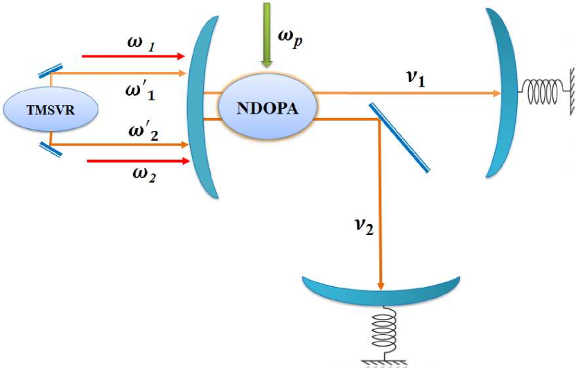
Figure 1: Schematics model of the driven doubly resonant optomechanical cavity system with intracavity non-degenerate optical parametric amplifier (NDOPA) and coupling two-mode squeezed vacuum reservoir (TMSVR). The details of the description are in the main text.

In this work, we considered a scheme that enhances the entanglement of two nano-mechanical oscillators induced via intracavity non-classical light and squeezed vacuum injection. In particular, we have considered a hybrid optomechanical system that consists of non-degenerate OPA inside a driven doubly resonant cavity coupled with two mechanical oscillators through radiation pressure. Moreover, the cavity is injected with a two-mode squeezed vacuum reservoir. Particularly, we focus on the impact of non-degenerate OPA and a two-mode squeezed vacuum reservoir controlling the degree of entanglement of mechanical oscillators in the system working in a good cavity limit for red-detuned laser drives. We have employed four entanglement quantifiers commonly used in continuous variable bipartite Gaussian states. These includes the Duan et al. [47], Mancini em et al. [48], the smallest symplectic eigenvalue [49], and the Hillery-Zubairy [50] entanglement quantification. Thus, we analyzed the degree of entanglement of two movable mirrors based on continuous variable bipartite Gaussian states’ entanglement quantification. The results show that the entanglement is significantly affected by the parametric phase and nonlinear gain of non-degenerate OPA, squeezing strength of squeezed vacuum reservoir, optomechanical cooperativity (laser driving power), and mechanical bath temperature (thermal excitation of phonons). Furthermore, the system under our investigation is believed to have a platform to realize quantum sensing and information processing.

The structure of this paper is as follows. The Hamiltonian of the model and the dynamics of the quantum Langevin equations with the steady-state values of operators and linearization are introduced In Sec. II. In Sec. III, we perform how to quantify entanglement from quadrature operators and introduce four entanglement quantifiers used as criteria to test inseparability in the bipartite system. In Sec. IV, the results of entanglement generated between the movable mirrors with their discussion are offered. Concluding remarks are given in Sec. V.

II Preliminaries

II.1 Model Hamiltonian and Dynamics

The model of our system under the current investigation comprises a pumped non-degenerate parametric amplifier (NDOPA) with second-order non-linearity in a doubly resonant Fabry-Pérot cavity each with length $L_{j}$ with two completely reflecting nano-mechanical mirrors each with masses $m_{j}$ oscillates with a frequency of $\Omega_{j}$. Additionally, a single-port fixed mirror is present, as illustrated in Fig. 1. The system is driven by two laser beams operating at frequencies $\omega_{1}$ and $\omega_{2}$ and coupled to a two-mode squeezed vacuum reservoir injected with central frequencies $\omega^{\prime}_{1}$ and $\omega^{\prime}_{2}$ at the fixed mirror. The NDOPA is pumped at a frequency $\omega_{p}=\nu_{1}+\nu_{2}$ which is then down-converted into correlated signal and idler photon pairs with frequencies $\nu_{1}$ and $\nu_{2}$. These frequencies are resonant with the corresponding cavity modes near $\nu_{j}$.

The total Hamiltonian $\hat{\mathcal{H}}$ of the system is

$$\hat{\mathcal{H}}=\hat{\mathcal{H}}_{o}+\hat{\mathcal{H}}_{m}+\hat{\mathcal{H}}_{om}+\hat{\mathcal{H}}_{d}+\hat{\mathcal{H}}_{p},$$ (1)

where $\hat{\mathcal{H}}_{o}=\sum^{2}_{j=1}\hbar\nu_{j}\hat{c}^{\dagger}_{j}\hat{c}_{j}$ and $\hat{\mathcal{H}}_{m}=\sum^{2}_{j=1}\hbar\Omega_{j}\hat{d}^{\dagger}_{j}\hat{d}_{j}$ the free Hamiltonian of the cavities and moving mirrors respectively with $\hat{c}_{j}(\hat{d}_{j})$ and $\hat{c}^{\dagger}_{j}(\hat{d}^{\dagger}_{j})$ describe the annihilation and creation operators of each cavity (mechanical) which satisfy the commutation relation $[\hat{\mathcal{O}}_{j},\hat{\mathcal{O}}_{j^{\prime}}]=[\hat{\mathcal{O}}^{\dagger}_{j},\hat{\mathcal{O}}^{\dagger}_{j^{\prime}}]=0,[\hat{\mathcal{O}}_{j},\hat{\mathcal{O}}^{\dagger}_{j^{\prime}}]=\delta_{jj^{\prime}}$ with $\hat{\mathcal{O}}=\hat{c},\hat{d}$, and $j,j^{\prime}=1,2$. The third term $\hat{\mathcal{H}}_{om}=-\sum^{2}_{j=1}\hbar g_{j}\hat{c}^{\dagger}_{j}\hat{c}_{j}(\hat{d}^{\dagger}_{j}+\hat{d}_{j})$ is the optomechanical interaction Hamiltonian due to radiation pressure [51] with $g_{j}=\frac{\nu_{j}}{L_{j}}\sqrt{\frac{\hbar}{2m_{j}\Omega_{j}}}$ is the single-photon optomechanical coupling. The fourth term $\hat{\mathcal{H}}_{d}=\sum^{2}_{j=1}i\hbar\big{(}\mathcal{E}_{j}e^{-i\omega_{j}t}\hat{c}^{\dagger}_{j}-\mathcal{E}^{*}e^{i\omega_{j}t}\hat{c}_{j}\big{)}$ is the Hamiltonian due to the interaction of the coherent laser driving fields and their corresponding cavity modes with $\mathcal{E}_{j}=|\mathcal{E}_{j}|e^{-i\phi_{j}}$, $\phi_{j}$ is the phase of laser drive, $|\mathcal{E}_{j}|=\sqrt{\frac{\kappa_{j}\mathcal{P}_{j}}{\hbar\omega_{j}}}$ is the magnitude of amplitude of driving laser which is related to the cavity driving laser power $\mathcal{P}_{j}$ and the cavity decay rate $\kappa_{j}$. The last term $\hat{\mathcal{H}}_{p}=i\hbar\Lambda(e^{i\theta}e^{-i\omega_{p}t}\hat{c}^{\dagger}_{1}\hat{c}^{\dagger}_{2}-e^{-i\theta}e^{i\omega_{p}t}\hat{c}_{1}\hat{c}_{2})$ [52] is the interaction Hamiltonian of the non-degenerate optical parametric amplifier and the cavity modes with $\Lambda$ is the non-linear parametric gain, which is proportional to the amplitude of its classical pumping field at parametric phase $\theta$.

Moreover, the Hamiltonian of the system in a rotating frame of unitary transformation operator $\hat{\mathcal{U}}=\exp{(i\hat{\mathcal{H}}^{\prime}t/\hbar)}$ for $\hat{\mathcal{H}}^{\prime}=\hbar\omega_{1}\hat{c}^{\dagger}_{1}\hat{c}_{1}+\hbar\omega_{2}\hat{c}^{\dagger}_{2}\hat{c}_{2}$ becomes

$$\begin{split}\hat{H}=&\sum^{2}_{j=1}\bigg{(}\hbar\big{[}\Delta^{\prime}_{j}-g_{j}(\hat{d}^{\dagger}_{j}+\hat{d}_{j})\big{]}\hat{c}^{\dagger}_{j}\hat{c}_{j}+\hbar\Omega_{j}\hat{d}^{\dagger}_{j}\hat{d}_{j}\\ &+i\hbar\big{[}\mathcal{E}_{j}\hat{c}^{\dagger}_{j}-\mathcal{E}^{*}_{j}\hat{c}_{j}\big{]}\bigg{)}\\ &+i\hbar\Lambda\big{[}\hat{c}^{\dagger}_{1}\hat{c}^{\dagger}_{2}e^{i\theta}e^{-i\Delta_{p}t}-\hat{c}_{1}\hat{c}_{2}e^{-i\theta}e^{i\Delta_{p}t}\big{]},\end{split}$$ (2)

where $\Delta^{\prime}_{j}=\nu_{j}-\omega_{j}$ and $\Delta_{p}=\omega_{p}-\omega_{1}-\omega_{2}=\Delta^{\prime}_{1}+\Delta^{\prime}_{2}$ are the detuning of cavity mode and NDOPA respectively.

To study the system dynamics, we employed the quantum Langevin equation (QLE), which includes different noises entering the system. The set of nonlinear QLEs obtained using the Hamiltonian $\hat{H}$ of Eq. (2) are given by

$$\begin{split}\frac{d}{dt}\hat{d}_{j}=&-i\Omega_{j}\hat{d}_{j}+ig_{j}\hat{c}^{\dagger}_{j}\hat{c}_{j}-\frac{\gamma_{j}}{2}\hat{d}_{j}+\sqrt{\gamma_{j}}\hat{d}^{in}_{j},\\ \frac{d}{dt}\hat{c}_{1}=&-i\Delta^{\prime}_{1}\hat{c}_{1}+ig_{1}\hat{c}_{1}(\hat{d}^{\dagger}_{1}+\hat{d}_{1})+\mathcal{E}_{1}\\ &+\Lambda e^{i\theta}e^{-i\Delta_{p}t}\hat{c}^{\dagger}_{2}-\frac{\kappa_{1}}{2}\hat{c}_{1}+\sqrt{\kappa_{1}}\hat{c}^{in}_{1},\\ \frac{d}{dt}\hat{c}_{2}=&-i\Delta^{\prime}_{2}\hat{c}_{2}+ig_{2}\hat{c}_{2}(\hat{d}^{\dagger}_{2}+\hat{d}_{2})+\mathcal{E}_{2}\\ &+\Lambda e^{i\theta}e^{-i\Delta_{p}t}\hat{c}^{\dagger}_{1}-\frac{\kappa_{2}}{2}\hat{c}_{2}+\sqrt{\kappa_{2}}\hat{c}^{in}_{2},\end{split}$$ (3)

where $\hat{c}^{in}_{j}$ and $\hat{d}^{in}_{j}$ are the annihilation operators related to input noises with zero-mean value associated with each cavity and moving mirror, respectively. We assume the mass of the movable mirrors are in nano-gram scale such that they oscillate at high-frequency associated with very high mechanical quality factors $(\mathcal{Q}_{j}=\Omega_{j}/\gamma_{j}\gg 1)$ and operate in ultra-cold temperatures. In this regard, the noise operator of each mirror can be taken as a Gaussian white-noise source, hence its evolution can be considered a Markovian process [53]. Thus, thermal noise operator $\hat{d}^{in}_{j}$ with nonzero delta correlation functions become [54] $\big{<}\hat{d}^{in,\dagger}_{j}(t)\hat{d}^{in}_{j}(t^{\prime})\big{>}=n_{j}\delta(t-t^{\prime})$ and $\big{<}\hat{d}^{in}_{j}(t)\hat{d}^{in,\dagger}_{j}(t^{\prime})\big{>}=(n_{j}+1)\delta(t-t^{\prime})$, with $n_{j}=\big{[}\exp([\hbar\Omega_{j}/(k_{B}T_{j})\big{]}-1)\big{]}^{-1}$ is the mean thermal excitation (phonon) number in the movable mirror at temperature $T_{j}$ and $k_{B}$ denotes the standard Boltzmann’s constant. On the other hand, the quantum fluctuation component $\hat{c}^{in}_{j}$ is injecting a broadband two-mode squeezed-vacuum reservoir with central frequency $\omega^{\prime}_{j}=\nu_{j}$. Thus, the noise operator $\hat{c}^{in}_{j}$ with zero mean value and its second-order correlation functions can be described by the correlation matrix as $\big{<}\hat{c}^{in,\dagger}_{j}(t)\hat{c}^{in}_{j}(t^{\prime})\big{>}=\mathcal{N}\delta(t-t^{\prime}),\big{<}\hat{c}^{in}_{j}(t)\hat{c}^{in,\dagger}_{j}(t^{\prime})\big{>}=(\mathcal{N}+1)\delta(t-t^{\prime}),\big{<}\hat{c}^{in}_{j}(t)\hat{c}^{in}_{j^{\prime}}(t^{\prime})\big{>}=\mathcal{M}\delta(t-t^{\prime})$, and $\big{<}\hat{c}^{in,\dagger}_{j}(t)\hat{c}^{in,\dagger}_{j^{\prime}}(t^{\prime})\big{>}=\mathcal{M}^{*}\delta(t-t^{\prime});j,j^{\prime}=1,2(j\neq j^{\prime})$ [55, 56]. Here $\mathcal{N}=\sinh^{2}{r}$ and $\mathcal{M}=e^{i\varphi}\cosh{(r)}\sinh{(r)}$ with $r$ and $\varphi$ are squeezing strength and phase of the squeezing respectively.

II.2 Linearization of quantum Langevin Equations

Strong enough laser intensities driving an optomechanical cavity enable the intracavity field to generate significant radiation pressure force to induce small perturbation on the movable mirror position. Consequently, we can investigate quantum effects through the linearized dynamics [51] with a zero mean quantum fluctuation operator $\delta\hat{\mathcal{O}}_{j}$ around the steady state value $\mathcal{O}^{s}_{j}=\big{<}\hat{\mathcal{O}}^{s}_{j}\big{>}$ such that $\hat{\mathcal{O}}_{j}=\mathcal{O}^{s}_{j}+\delta\hat{\mathcal{O}}_{j}$. At steady-state, the c-number form of the operators in Eq. (3) become

$$\begin{split}c^{s}_{1}=&\frac{2\mathcal{E}_{1}(\kappa_{2}-2i\Delta_{2})}{(\kappa_{1}+2i\Delta_{1})(\kappa_{2}-2i\Delta_{2})-4\Lambda^{2}},\\ c^{s}_{2}=&\frac{2\mathcal{E}_{2}(\kappa_{1}-2i\Delta_{1})}{(\kappa_{2}+2i\Delta_{2})(\kappa_{1}-2i\Delta_{1})-4\Lambda^{2}},\\ d^{s}_{j}=&\frac{2ig_{j}|c^{s}_{j}|^{2}}{\gamma_{j}+2i\Omega_{j}}.\end{split}$$ (4)

Here we neglect the high-frequency terms in $c^{s}_{j}$, and the expression $\Delta_{j}=\Delta^{\prime}_{j}-g_{j}(d^{s*}_{j}+d^{s}_{j})$ is the effective cavity-laser field detuning of each optomechanical cavity caused by radiation pressure. The linearized form of the quantum fluctuations Langevin equations of Eq. (3) is provided in Eq. (21) and Eq. (23) as non-rotating and rotating wave approximation (RWA) respectively.

Furthermore, the dynamics can be considered adiabatically in the resolved sideband regime for a high mechanical quality factor ($\Omega_{j}\gg\kappa_{j}\gg\gamma_{j})$ and in the very weak coupling limit $(\mathcal{G}_{j}\ll\kappa_{j})$. Thus, in such conditions, the cavity mode dynamics can follow the mechanical modes, and we can eliminate the cavity mode dynamics such that the photons leave the cavity with a lower interaction with the moving mirrors, allowing an optimal quantum state transfer [29]. In this regard, we can set in large time approximation that the time rate of each of the cavity modes fluctuation operators set $\frac{d}{dt}\delta\tilde{c}_{j}=0$ in Eq. (23). Thus, we obtain the linearized dynamical quantum Langevine equations as if the system with two movable mirrors as

$$\begin{split}\frac{d}{dt}\delta\tilde{d}_{1}&=-\frac{\Upsilon_{1}}{2}\delta\tilde{d}_{1}+\chi\delta\tilde{d}^{\dagger}_{2}+\tilde{f}_{1},\\ \frac{d}{dt}\delta\tilde{d}_{2}&=-\frac{\Upsilon_{2}}{2}\delta\tilde{d}_{2}+\chi\delta\tilde{d}^{\dagger}_{1}+\tilde{f}_{2}.\end{split}$$ (5)

Here the $j^{th}$ mechanical mode effective damping rate is $\Upsilon_{j}=\gamma_{j}+\Gamma_{j}$ with $\Gamma_{1}=\frac{\mathcal{G}_{1}^{2}\kappa_{2}}{\mathcal{K}}$ and $\Gamma_{2}=\frac{\mathcal{G}_{2}^{2}\kappa_{1}}{\mathcal{K}}$ effective damping rate induced by the radiation pressure, with $\mathcal{K}=\frac{\kappa_{1}\kappa_{2}}{4}-{\Lambda}^{2}$, $\chi=\frac{\mathcal{G}_{1}\mathcal{G}_{2}}{\mathcal{K}}\Lambda e^{i\theta}$ is the effective coupling strength between the two mechanical modes induced by the driving lasers and NDOPA, and $\tilde{f}_{1}=a_{1}\sqrt{\kappa_{1}}\tilde{c}^{in}_{1}+b_{1}\sqrt{\kappa_{2}}\tilde{c}^{in,\dagger}_{2}+\sqrt{\gamma_{1}}\tilde{d}^{in}_{1}$, $\tilde{f}_{2}=a_{2}\sqrt{\kappa_{2}}\tilde{c}^{in}_{2}+b_{2}\sqrt{\kappa_{1}}\tilde{c}^{in,\dagger}_{1}+\sqrt{\gamma_{2}}\tilde{d}^{in}_{2}$ are the quantum Langevine forces to the movable mirrors with $a_{1}=\frac{i\mathcal{G}_{1}\kappa_{2}}{2\mathcal{K}}$, $b_{1}=\frac{i\mathcal{G}_{1}{\Lambda}e^{i\theta}}{\mathcal{K}}$, $a_{2}=\frac{i\mathcal{G}_{2}\kappa_{1}}{2\mathcal{K}}$, $b_{2}=\frac{i\mathcal{G}_{2}{\Lambda}e^{i\theta}}{\mathcal{K}}$.

In the presence of the NDOPA ($\Lambda\neq 0$) and the cavity driving laser field ($\mathcal{G}_{j}\neq 0$), it is noted that in Eq. (5), $\frac{d}{dt}\delta\tilde{d}_{j}$ depends on $\delta\tilde{d}^{\dagger}_{j^{\prime}}$ and $\tilde{c}^{in,\dagger}_{j^{\prime}}$ that induce quantum state transfer to the movable mirrors to be in an entangled state. Therefore, the NDOPA in the cavity or the squeezed noise injection causes a non-classical correlation between the two movable mirrors.

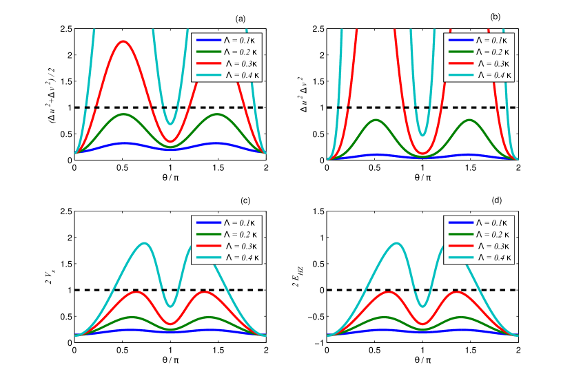
Figure 2: Plots of entanglement quantification via (a) Duan $et$ $al.$ $(\Delta u^{2}+\Delta v^{2})/2$, (b) Mancini $et$ $al.$ $\Delta u^{2}\Delta v^{2}$, (c) smallest symplectic eigenvalue $(2V_{s})$, and (d) Hillery-Zubairy $(2E_{HZ})$ versus parametric phase of NDOPA for different parametric gain when $r=1$, $T=42\mu K(n=0.5)$, $\mathcal{P}=0.3mW(C=62.5,\mathcal{G}=0.1\kappa)$. The other parameters are listed in the main text.

III Entanglement Quantification

To quantify entanglement between the movable mirrors using Eq. (5), we introduce relevant quadrature operators for the mechanical modes. Specifically, the quadrature operators $\delta\tilde{Q}_{j}=\frac{1}{\sqrt{2}}(\delta\tilde{d}^{\dagger}_{j}+\delta\tilde{d}_{j})$ and $\delta\tilde{P}_{j}=\frac{i}{\sqrt{2}}(\delta\tilde{d}^{\dagger}_{j}-\delta\tilde{d}_{j})$, which correspond to the position and momentum quadrature operators of the mechanical modes, respectively. Here, $\delta\tilde{d}_{j}$ represents the fluctuation of the mechanical annihilation operator around its steady-state value. Similarly, the corresponding input noise quadrature operators are $\tilde{Q}^{in}_{j}=\frac{1}{\sqrt{2}}(\tilde{f}^{\dagger}_{j}+\tilde{f}_{j})$ and $\tilde{P}^{in}_{j}=\frac{i}{\sqrt{2}}(\tilde{f}^{\dagger}_{j}-\tilde{f}_{j})$, where $\tilde{f}_{j}$ denotes the noise operator associated with the mechanical mode $j$. The adiabatic approximation allows the dynamical equations of the system to be simplified into a compact form, as shown below:

$$\frac{d}{dt}\mathcal{Z}(t)=\mathcal{B}\mathcal{Z}(t)+\mathcal{S}(t).$$ (6)

where $\mathcal{Z}(t)=\big{(}\delta{\tilde{Q}}_{1},\delta{\tilde{P}}_{1},\delta{\tilde{Q}}_{2},\delta{\tilde{P}}_{2}\big{)}^{T}$ is the vector of the quadrature operators, encompassing both the mechanical position and momentum fluctuations, $\mathcal{S}(t)=\big{(}\tilde{Q}^{in}_{2},\tilde{P}^{in}_{2},\tilde{Q}^{in}_{2},\tilde{P}^{in}_{2}\big{)}^{T}$ represents the vector of noise terms, which includes the contributions from the input noise quadratures, and the drift matrix, $\mathcal{B}$, which contains the system’s information, is given by:

$$\mathcal{B}=\begin{pmatrix}-\Upsilon_{1}/2&0&|\chi|\cos{\theta}&|\chi|\sin{\theta}\\ 0&-\Upsilon_{1}/2&|\chi|\sin{\theta}&-|\chi|\cos{\theta}\\ |\chi|\cos{\theta}&|\chi|\sin{\theta}&-\Upsilon_{2}/2&0\\ |\chi|\sin{\theta}&-|\chi|\cos{\theta}&0&\Upsilon_{2}/2\\ \end{pmatrix}.$$ (7)

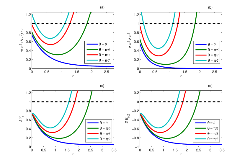
Figure 3: Plots of (a) Duan $et$ $al.$ $(\Delta u^{2}+\Delta v^{2})/2$, (b) Mancini $et$ $al.$ $\Delta u^{2}\Delta v^{2}$, (c) smallest symplectic eigenvalue $(2V_{s})$, and (d) Hillery-Zubairy $(2E_{HZ})$ entanglement quantifiers versus squeezing strength $r$ for different parametric phases when $\Lambda=0.2\kappa$. The other parameters are the same as in Fig. 2.

We analyze the system’s stability in Appendix B. The system is in a stable regime if and only if the condition $\Lambda<\frac{1}{2}\sqrt{\kappa_{1}\kappa_{2}}$ is satisfied. Furthermore, the formal solution of the matrix equation Eq. (6) is obtained as

$$\mathcal{Z}(t)=\mathcal{Z}(0)e^{\mathcal{B}t}+\int_{0}^{t}e^{\mathcal{B}t^{\prime}}\mathcal{Z}(t-t^{\prime})dt^{\prime},$$ (8)

where $\mathcal{Z}(0)$ is the vector of the initial values of the components. Since the noises $\tilde{c}^{in}_{j}$ and $\tilde{d}^{in}_{j}$ are $\delta$-correlated, they describe a Markovian process. For a stable system, the steady-state covariance matrix $\mathcal{R}$ can therefore be determined by solving the Lyapunov equation [54].

$$\mathcal{BR}+\mathcal{RB}^{T}=-\mathcal{F},$$ (9)

where $\mathcal{F}$ is the diffusion matrix. The detailed analytic expressions of the elements of the matrices $\mathcal{F}$ and $\mathcal{R}$ are derived in Appendix  C and the expression of their elements are provided in Eq. (25) and Eq. (28) respectively.

By definition, a quantum state $\hat{\rho}_{AB}$ of a bipartite system is said to be not entangled (separable) if and only if $\hat{\rho}_{AB}$ can be written as a convex combination of product states.

$$\hat{\rho}_{AB}=\sum_{k}p_{k}\hat{\rho}_{kA}\otimes\hat{\rho}_{kB},$$ (10)

where $\hat{\rho}_{kA}$ and $\hat{\rho}_{kB}$ are the density operators of mode-A and mode-B, respectively, with the probability $\sum_{k}p_{k}$ = 1 for (0$\leq$ $p_{k}$ $\leq$ 1). We address four different entanglement quantifiers to investigate the degree of entanglement for the bipartite Gaussian state of the two moving mirrors. These entanglement quantifiers are mostly employed in continuous variable bipartite Gaussian states here we include the Duan $et$ $al.$ [47], Mancini $et$ $al.$ [48], the smallest symplectic eigenvalue [49], and the Hillery-Zubairy [50] entanglement quantification criteria.

III.1 Duan et al

To apply the Duan $et$ $al.$ quantifier, a maximally entangled continuous-variable Gaussian state can be expressed as a co-eigenstate of a pair of Einstein-Podolsky-Rosen (EPR)-like quadrature operators [57] $u$ and $v$ defined as

$$\begin{split}u&=\delta\tilde{Q}_{1}+\delta\tilde{Q}_{2},\\ v&=\delta\tilde{P}_{1}-\delta\tilde{P}_{2},\end{split}$$ (11)

It is also possible to define the EPR-like quadrature pair as $\delta\tilde{Q}_{1}-\delta\tilde{Q}_{2}$ and $\delta\tilde{P}_{1}+\delta\tilde{P}_{2}$; however, the former is appropriate for our case. Thus, the non-vanishing variances (second moment) of the quadrature operators $u$ and $v$ at steady state we obtain

$$\Delta u^{2} = \big{<}(\delta\tilde{Q}_{1})^{2}\big{>}+\big{<}(\delta\tilde{Q}_{2})^{2}\big{>}+2\big{<}\delta\tilde{Q}_{1}\delta\tilde{Q}_{2}\big{>}$$

$$= \mathcal{R}_{11}+\mathcal{R}_{33}+2\mathcal{R}_{13},$$

and

$$\Delta v^{2} = \big{<}(\delta\tilde{P}_{1})^{2}\big{>}+\big{<}(\delta\tilde{P}_{2})^{2}\big{>}-2\big{<}\delta\tilde{P}_{1}\delta\tilde{P}_{2}\big{>}$$

$$= \mathcal{R}_{11}+\mathcal{R}_{33}+2\mathcal{R}_{13}.$$

Thus, we can rewrite the sum of quadrature variances in terms of covariance elements as

$$\Delta u^{2}+\Delta v^{2}=2(\mathcal{R}_{11}+\mathcal{R}_{33}+2\mathcal{R}_{13}).$$ (12)

The system’s mechanical modes are entangled and in a two-mode squeezed state, provided that the following inequality is satisfied. [47]

$$(\Delta u^{2}+\Delta v^{2})/2=\mathcal{R}_{11}+\mathcal{R}_{33}+2\mathcal{R}_{13}<1.$$ (13)

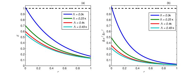
Figure 4: Plots of entanglement quantification via (a) Duan $et$ $al.$, the smallest symplectic eigenvalue, Hillery-Zubairy entanglement criteria where $E=(\Delta u^{2}+\Delta v^{2})/2,2V_{s},1+2E_{HZ}$; and (b) Mancini $et$ $al.$ entanglement criteria $\Delta u^{2}\Delta v^{2}$ versus versus squeezing strength $r$ for different parametric gain when $\theta=0$. The other parameters are the same as in Fig. 2.

III.2 Mancini et al.

With similar definitions for EPR quadrature operators as described in Eq. (11) for Duan $et$ $al.$ entanglement quantifier, we have another entanglement quantifier that is sufficient for the Gaussian bipartite system inseparability if the products of the quadrature variances of $\Delta u^{2}$ and $\Delta v^{2}$ satisfy Mancini $et$ $al.$ quantifier [48]. Thus, we have the inseparability condition as

$$\Delta u^{2}\Delta v^{2}=(R_{11}+R_{33}+2R_{13})^{2}<1.$$ (14)

III.3 Logarithmic negativity

Another relevant method that reveals the existence of entanglement in a bipartite state is logarithmic negativity, in which the product density operator for a separable composite state has a positive partial transpose [58, 59]. Notably, the logarithmic negativity for a continuously variable system is defined as

$$E_{n}=\max[0,-\ln(2V_{s})],$$ (15)

in which $V_{s}$ is the smallest eigenvalue of the symplectic matrix [49]. In line with this, the two mechanical modes are said to be entangled if and only if $E_{n}>0$ or $2V_{s}<1$. In this regard, the smallest symplectic eigenvalue $V_{s}$ of the partial transpose of the $4\times 4$ covariance matrix $\mathcal{R}$ is found to have the form

$$V_{s}=\sqrt{\frac{\zeta-\sqrt{\zeta^{2}-4\det\mathcal{R}}}{2}},$$ (16)

with $\zeta=\det\mathcal{R}_{1}+\det\mathcal{R}_{2}-2\det\mathcal{R}_{3}=\mathcal{R}^{2}_{11}+\mathcal{R}^{2}_{33}+2(\mathcal{R}^{2}_{13}+\mathcal{R}^{2}_{14})$ and $\det\mathcal{R}=\big{(}\mathcal{R}_{11}\mathcal{R}_{33}-\mathcal{R}^{2}_{13}\big{)}^{2}$.

III.4 Hillery-Zubairy

The Hillery-Zubairy (HZ) inseparablity criterion [50] that relies on second-order moments of the mechanical-mode operators and the states of a bipartite system is said to be entangled when the following relation holds:

$$E_{HZ}=\big{[}\big{<}\delta\tilde{d}^{\dagger}_{1}\delta\tilde{d}_{1}\big{>}\big{<}\delta\tilde{d}^{\dagger}_{2}\delta\tilde{d}_{2}\big{>}\big{]}^{1/2}-|\big{<}\delta\tilde{d}_{1}\delta\tilde{d}_{2}\big{>}|<0.$$ (17)

Utilizing the definition of creation $\delta\tilde{d}^{\dagger}_{j}$ and annihilation operators $\delta\tilde{d}_{j}$ in terms of Hermitian quadrature $\delta\tilde{Q}_{j}$ and $\delta\tilde{P}_{j}$, we obtain

$$\delta\tilde{d}^{\dagger}_{j}\delta\tilde{d}_{j}=\frac{1}{2}\big{[}\delta\tilde{Q}_{j}\delta\tilde{Q}_{j}+\delta\tilde{P}_{j}\delta\tilde{P}_{j}-1\big{]},$$ (18)

and with a similar procedure we obtain

$$\delta\tilde{d}_{j}\delta\tilde{d}_{j^{\prime}}=\frac{1}{2}\big{[}\delta\tilde{Q}_{j}\delta\tilde{Q}_{j^{\prime}}-\delta\tilde{P}_{j}\delta\tilde{P}_{j^{\prime}}+i(\delta\tilde{Q}_{j}\delta\tilde{P}_{j^{\prime}}+\delta\tilde{P}_{j}\delta\tilde{Q}_{j^{\prime}})\big{]}.$$ (19)

In terms of the covariance matrix elements at steady state, the HZ entanglement criterion Eq. (17) considering Eq. (18) and Eq. (19) we obtain

$$E_{HZ}=\frac{1}{2}[(2\mathcal{R}_{11}-1)(2\mathcal{R}_{33}-1)]^{1/2}-|\mathcal{R}_{13}+i\mathcal{R}_{14}|<0,$$

This entanglement criterion can be rearranged and a bipartite system inseparability can also be rewritten as $2E_{HZ}<0$, or $1+2E_{HZ}<1$.

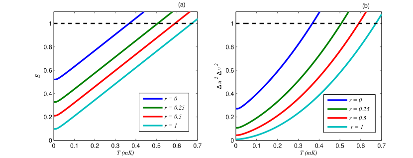
Figure 5: Plots of entanglement quantification via (a) Duan $et$ $al.$, the smallest symplectic eigenvalue, Hillery-Zubairy where $E=(\Delta u^{2}+\Delta v^{2})/2,2V_{s},1+2E_{HZ}$; and (b) Mancini $et$ $al.$ entanglement quantifiers $\Delta u^{2}\Delta v^{2}$ versus temperature $T$ of mechanical baths for different squeezing strength $r$ when $\Lambda=0.49\kappa$ and $\theta=0$. The other parameters are the same as in Fig. 2.

IV Results and Discussion

The degree of entanglement and its quantification can be realized in the two mechanical modes at steady-state. To achieve this, we select feasible parameters based on recent experiments in the optomechanical system [60]. For simplicity, we take identical parameters for field-mirror pairs such that the wavelength of the driving lasers $\lambda=1064nm(\omega_{1}/2\pi=\omega_{2}/2\pi=2.82\times 10^{14}Hz)$, frequency of the mechanical oscillators $\Omega_{1}/2\pi=\Omega_{2}/2\pi=947\times 10^{3}Hz$, masses of the movable mirrors $m_{1}=m_{2}=145ng$, the length of the cavities $L_{1}=L_{2}=25mm$, the cavity decay rates $\kappa_{1}/2\pi=\kappa_{2}/2\pi=\kappa/2\pi=215\times 10^{3}Hz$, and the mechanical modes damping rates $\gamma_{1}/2=\gamma_{2}/2\pi=\gamma/2\pi=140Hz$. In addition, we consider equal bath temperature, $T_{1}=T_{2}=T(n_{1}=n_{2}=n)$, and the value phase squeezing is fixed at $\varphi=0$. Moreover, we utilize equal laser driving powers, $\mathcal{P}_{1}=\mathcal{P}_{2}=\mathcal{P}$ that yield identical optomechanical coupling rates, $\mathcal{G}_{1}=\mathcal{G}_{2}=\mathcal{G}$. Here we define the optomechanical cooperativity as $C=\frac{4\mathcal{G}^{2}}{\gamma\kappa}$ that is directly proportional to $\mathcal{P}$.

Accordingly, utilizing the covariance matrix elements in Eq. (28), we quantify the degree of nano-mechanical resonators using different kinds of entanglement quantifiers based on Eq. (13), Eq. (14), Eq. (16) and Eq. (III.4). The plots of the entanglement quantification results depend on the squeezing strength ($r$) of two-mode squeezed field injection, the parametric phase ($\theta$) and gain of NDOPA ($\Lambda$), the thermal decoherence effect of mechanical baths (temperature $T$ and phonon number $n$), and the optomechanical cooperativity ($C$).

Even though there is no direct interaction between the movable mirrors, it can be conceived that the quantum behavior of the two-mode output of NDOPA could be transferred to the oscillations of the movable mirrors. The mechanical oscillators in our system were not directly coupled initially; both the injected two-mode squeezed vacuum fields to the system and the two-mode squeezed intracavity radiation emitted from NDOPA are jointly found to be transferred to the movable mirrors via the effective coupling between the two mechanical modes induced by the driving lasers and NDOPA system, which leads to the non-classical effects generation between the mechanical modes.

In Figs. 2(a) - 2(d), the entanglement versus normalized parametric phase ($\theta/\pi$) for different nonlinear gains are plotted. In these plots, we observe that increasing the nonlinear gain of NDOPA enhances the degree of entanglement at $\theta=0$. On the other hand, the degree of entanglement decreases at higher values of the parametric phases, far above $\theta=0$ for larger nonlinear gain. In contrast, the lower nonlinear gains show higher entanglement and satisfy the inseparability criteria for all ranges of parametric phases. For $\Lambda=0.1\kappa$ and $\Lambda=0.2\kappa$ in Figs. 2(a) - 2(b), as well as for $\Lambda=0.1\kappa$, $\Lambda=0.2\kappa$ and $\Lambda=0.3\kappa$ in Figs. 2(c) - 2(d), as the parametric gain increases up to $\theta=\pi/2$, the degree of entanglement decreases. Furthermore, in all cases of the entanglement quantifiers at the parametric phase $\theta=\pi$, it is depicted that the degree of entanglement is reduced as the nonlinear gain increases. Moreover, for $\Lambda=0.3\kappa$, the Duan $et$ $al.$ and Mancini $et$ $al.$ entanglement quantifiers fail to capture quantum correlation for a wider range of parametric phases. However, the logarithmic negativity with the smallest symplectic eigenvalue and Hillery-Zubairy quantifiers can capture the entanglement at $\Lambda=0.3\kappa$.

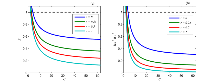
Figure 6: Plots of entanglement quantification of (a) Duan $et$ $al.$, the smallest symplectic eigenvalue, Hillery-Zubairy where $E=(\Delta u^{2}+\Delta v^{2})/2,2V_{s},1+2E_{HZ}$; and (b) Mancini $et$ $al.$ $\Delta u^{2}\Delta v^{2}$ versus optomechanical cooperativity (C) for different squeezing strength $r$ when $\Lambda=0.49\kappa$, $\theta=0$. The other parameters are the same as in Fig. 2.

In Figs. 3(a) - 3(b), the entanglement versus the squeezing strength $r$ for different parametric phases are plotted. It is clearly shown that as the parametric phase increases to $\pi/2$, the degree of entanglement decreases. For $r=0$, the Duan $et$ $al.$ and Mancini $et$ $al.$ entanglement quantifiers are sensitive to the parametric phase variation, whereas the smallest symplectic eigenvalue and Hillery-Zubairy entanglement quantifiers are unresponsive to parametric phase changes. Corresponding to each parametric phase, as the squeezing strength increases, the degree of entanglement increases to an optimal degree of entanglement and then decreases except at $\theta=0$. Moreover, the symplectic smallest eigenvalue and Hillery-Zubairy entanglement quantifiers can capture entanglement at a higher squeezing strength than the Duan $et$ al. and Mancini $et$ $al.$ entanglement quantifiers. A wider range of the squeezing strength $r$ of injected squeezed fields corresponded to lower values of parametric phases with enhanced entanglement. At $\theta=0$, the highest degree of entanglement quantification is obtained in the four entanglement quantifiers.

It is also a well-established fact that the external radiation that pumps NDOPA induces coherent superposition, which is responsible for a strong dependence of the quantum correlation properties of the radiation on the non-linear gain $\Lambda$ proportional to the amplitude of the pumping field. In Figs. 4(a) - 4(b), in the absence of the injected squeezed vacuum fields (squeezing $r=0$) and the NDOPA (nonlinear gain $\Lambda=0$), the mechanical-modes entanglement take the minimal value. However, in the existence of NDOPA, the generated NDOPA-correlated photons cause the entanglement of the mechanical modes for $r=0$. Moreover, the joint effect of NDOPA and injected non-classical squeezed fields makes the entanglement more robust for $r\neq 0$. It is clearly shown that the entanglement is enhanced as the nonlinear gain is increased. Moreover, the degree of entanglement also becomes more robust as the strength of squeezing $r$ increases towards $r=1$. This can be explained by the fact that the degree of entanglement is very directly related to the effective couplings between the two mechanical modes, $\chi$, so that the entanglement can be enhanced as the effective couplings rely directly on the respective terms, $\Lambda$. Moreover, the effect of NDOPA is more significant for lower squeezing strength, whereas as $r$ goes to 1, the variation of NDOPA effect becomes faint. In addition, the Duan $et$ $al.$, the smallest symplectic eigenvalue, and the Hillery-Zubairy entanglement quantifiers show similar entanglement quantification features, unlike the Mancini $et$ $al.$ criteria.

It is also essential to know the effects of the temperature of the mechanical bath, which is the resource for decoherence and diminishes entanglement. To this end, the plot of entanglement as a function of the temperature ($T$) of mechanical baths is shown in Figs. 5(a) - 5(b) for different squeezing strengths ($r$) at fixed non-linear gain near the threshold value $\Lambda=0.49\kappa$. Here, we examine the effect of varying the squeezing strengths on the degree of entanglement quantification of mechanical modes. It is depicted that as the squeezing strength increases, the entanglement becomes more robust against temperature. This is due to the higher mechanical bath temperature increasing vibration and enhancing phonon numbers directly related to thermal decoherence, significantly degrading the coherence vital for entanglement. Moreover, as the temperature rises for a given squeezing strength, the degree of entanglement decreases. In addition, the four entanglement quantifiers display equal robustness against temperature for various squeezing strengths. However, the plots with Mancini $et$ $al.$ entanglement quantifier have a higher degree of entanglement even at $T=0K$ than the rest.

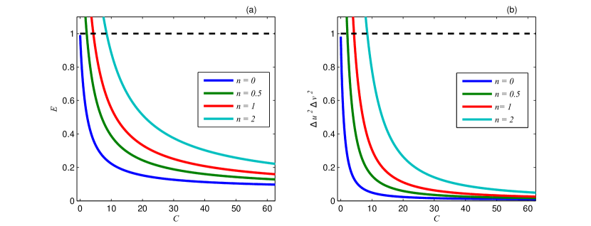
Figure 7: Plots of (a) Duan $et$ $al.$, the smallest symplectic eigenvalue, Hillery-Zubairy where $E=(\Delta u^{2}+\Delta v^{2})/2,2V_{s},1+2E_{HZ}$; and (b) Mancini $et$ $al.$ $\Delta u^{2}\Delta v^{2}$ entanglement quantifiers versus optomechanical cooperativity (C) for different phonon number $n$ when squeezing strength $r=1$, $\Lambda=0.49\kappa$, $\theta=0$. The other parameters are the same as in Fig. 2.

Moreover, the effect of cooperativity $C$ on various entanglement criteria is plotted in Figs. 6(a) - 6(b) and Figs. 7(a) - 7(b) for different squeezing strengths $r$ and thermal phonon numbers $n$, respectively. In both Figs. 6 and Figs. 7, it is clearly shown that as the optomechanical cooperativity increases, the degree of entanglement is drastically enhanced for lower cooperativity while the degree of entanglement is slightly increasing for higher cooperativity. It is also shown that the quantity of entanglement is enhanced due to the effect of increasing $r$ whereas increasing the phonon number $n$ is negatively related to the degree of entanglement. Furthermore, the effects of cooperativity can be explained via the degree of entanglement related directly to the square of the strength of the optomechanical coupling $\mathcal{G}^{2}$ due to the radiation pressure or directly proportional to the laser driving power $\mathcal{P}$ so that the entanglement can be enhanced. In addition, the many-photon coupling $\mathcal{G}$ depends directly on the amplitude of the driving laser, resulting in an enhancement of intracavity photon numbers. In addition, the minimum cooperativity required to birth entanglement is identical in all considered entanglement criteria corresponding to each squeezing strength in Fig. 6 and thermal photon number in Fig. 7. In Fig. 6, it is shown that the smaller the squeezing strength, the greater the cooperativity requirement for the mechanical modes to display a non-classical effect. Similarly, in Fig. 7, the smaller the thermal phonon number corresponds to a lower quantity of cooperativity.

In summary, regarding the connection among the entanglement quantifiers used to quantify the entanglement of mechanical oscillators in our system, we illustrated four kinds of entanglement quantifiers in Figs. 2 - 7 for the same set of parameters to the corresponding figures. Although the four quantifiers show qualitatively similar behavior as a function of parametric pump phase and squeezing strength, there is a notable disparity among the entanglement capture. For example, in the presence of a parametric phase effect, the two quantifiers Duan $et$ $al.$ and Mancini $et$ $al.$ exhibit entanglement for an identical range of parametric phases and squeezing strength. In contrast, the smallest symplectic eigenvalue and HZ quantifiers have displayed qualitatively and quantitatively similar for identical ranges, as shown in Fig. 2 and Fig. 3. The smallest symplectic eigenvalue and HZ quantifiers show entanglement for a wider squeezing strength range than the Duan $et$ $al.$ and Mancini $et$ $al.$ quantifiers. In addition, we note that the smallest symplectic eigenvalue and HZ quantifiers are stronger in capturing entanglement in the presence of parametric phase than the Duan $et$ $al.$ and Mancini $et$ $al.$ quantifiers to capture entanglement in our scheme. Furthermore, in the zero parametric pumping phase, all four quantifiers display similar behavior entanglement via increasing the nonlinear gain, the temperature of the mechanical bath, squeezing strength, and thermal excitation as in Fig. 4, Fig. 5, Fig. 6, and Fig. 7 respectively. However, the three quantifiers, Duan $et$ $al.$, the smallest symplectic eigenvalue and HZ quantifiers, are quantitatively identical entanglement, unlike Mancini $et$ $al.$ quantifiers, which exhibit the strongest degree of entanglement as in Figs.  4 - 7. Furthermore, for an optomechanical system, the entanglement can be realized by taking recent experimental feasible parameters [60] and capturing the covariance matrix elements of the mechanical modes through the experimental technique as in Ref.[54] via varying the phase of local oscillators.

V Conclusions

We investigated a driven hybrid optomechanical doubly resonant cavity coupled to two nano-mechanical mirrors, incorporating a non-degenerate optical parametric amplifier (NDOPA) with a second-order nonlinear crystal medium and a two-mode squeezed vacuum injection. The system operates within a weak coupling regime and a good cavity limit. We utilized the covariance matrix elements in the four kinds of entanglement quantifiers, which are sufficient conditions for continuous variable Gaussian bipartite states, to quantify entanglement across various system parameters in the two nano-mechanical mirrors. Our study reveals that the degree of entanglement is significantly influenced by factors such as squeezing strength, parametric pumping phase, nonlinear gain of the NDOPA, optomechanical cooperativity, and temperature. Our results indicate that an optimal entanglement occurs at a specific parametric phase where noise is drastically suppressed. At this phase, increasing the strength of the squeezing parameter for the injected squeezed state enhances the robustness of the entanglement, pushing it towards its ideal limit. In addition, raising the nonlinear parametric gain further elevates the entanglement between the two mechanical mirrors. Furthermore, coupling a two-mode squeezed vacuum reservoir (TMSVR) to the system demonstrates robustness against the temperature of mechanical baths. At higher thermal noise levels, entanglement is enhanced by suppressing thermal noise through increased optomechanical cooperativity. Consequently, the degree of entanglement can be controlled via several parameters, suggesting that our model has potential applications in quantum metrology and information processing.

Appendices

APPENDIX A Linearization and rotating wave approximation

In this section for completeness, we derive the linearized form of quantum Langevine equations in rotating wave approximation. For a sufficiently strong laser driving power we can assume that $|c^{s}_{j}|\gg 1$ such that the quantum Langevin equations of Eq. (3) can be safely linearized by dropping higher order terms, $\delta\hat{c}^{\dagger}_{j}\delta\hat{c}_{j}$, and $\delta\hat{c}_{j}(\delta\hat{d}^{\dagger}_{j}+\delta\hat{d}_{j})$. Hence, the dynamics of the quantum fluctuations become

$$\begin{split}\frac{d}{dt}\delta\hat{d}_{j}=&-\big{(}\frac{\gamma_{j}}{2}+i\Omega_{j}\big{)}\delta\hat{d}_{j}+i\mathcal{G}_{j}(\delta\hat{c}^{\dagger}_{2}+\delta\hat{c}_{j})\\ &+\sqrt{\gamma_{j}}\hat{d}^{in}_{j},\\ \frac{d}{dt}\delta\hat{c}_{1}=&-\big{(}\frac{\kappa_{1}}{2}+i\Delta_{1}\big{)}\delta\hat{c}_{1}+i\mathcal{G}_{1}(\delta\hat{d}^{\dagger}_{1}+\delta\hat{d}_{1})\\ &+\Lambda e^{i\theta}e^{-i\Delta_{p}t}\delta\hat{c}^{\dagger}_{2}+\sqrt{\kappa_{1}}\hat{c}^{in}_{1},\\ \frac{d}{dt}\delta\hat{c}_{2}=&-\big{(}\frac{\kappa_{2}}{2}+i\Delta_{2}\big{)}\delta\hat{c}_{2}+i\mathcal{G}_{2}(\delta\hat{d}^{\dagger}_{2}+\delta\hat{d}_{2})\\ &+\Lambda e^{i\theta}e^{-i\Delta_{p}t}\delta\hat{c}^{\dagger}_{1}+\sqrt{\kappa_{2}}\hat{c}^{in}_{2}.\end{split}$$ (21)

where $\mathcal{G}_{j}=g_{j}|c^{s}_{j}|$ is the effective optomechanical coupling rate that depends on the power $\mathcal{P}_{j}$ of the input laser. Here we take the amplitude of the cavity mode $c^{s}_{j}$ to be real via adjusting the phase $\phi_{j}$ of the laser drive field.

Furthermore, we introduce slowly varying operators $\delta\tilde{c}_{j}=\delta\hat{c}_{j}e^{i\Delta_{j}t},\tilde{c}^{in}_{j}=\hat{c}^{in}_{j}e^{i\Delta_{j}t}$, $\delta\tilde{d}_{j}=\delta\hat{d}_{j}e^{i\Omega_{j}t}$ and $\tilde{d}^{in}_{j}=\hat{d}^{in}_{j}e^{i\Omega_{j}t}$ into Eq. (21), the dynamics of the linearized quantum Langevine equations become

$$\begin{split}\frac{d}{dt}\delta\tilde{d}_{j}=&-\frac{\gamma_{j}}{2}\delta\tilde{d}_{j}+i\mathcal{G}_{j}(\delta\tilde{c}^{\dagger}_{j}e^{i(\Delta_{j}+\Omega_{j})t}+\delta\tilde{c}_{j}e^{-i(\Delta_{j}-\Omega_{j})t})\\ &+\sqrt{\gamma_{j}}\tilde{d}^{in}_{j},\\ \frac{d}{dt}\delta\tilde{c}_{1}=&-\frac{\kappa_{1}}{2}\delta\tilde{c}_{1}+i\mathcal{G}_{1}(\delta\tilde{d}^{\dagger}_{1}e^{i(\Delta_{1}+\Omega_{1})t}+\delta\tilde{d}_{1}e^{i(\Delta_{1}-\Omega_{1})t})\\ &+\Lambda e^{i\theta}\delta\tilde{c}^{\dagger}_{2}+\sqrt{\kappa_{1}}\tilde{c}^{in}_{1},\\ \frac{d}{dt}\delta\tilde{c}_{2}=&-\frac{\kappa_{2}}{2}\delta\tilde{c}_{2}+i\mathcal{G}_{2}(\delta\tilde{d}^{\dagger}_{2}e^{i(\Delta_{2}+\Omega_{2})t}+\delta\tilde{d}_{2}e^{i(\Delta_{2}-\Omega_{2})t})\\ &+\Lambda e^{i\theta}\delta\tilde{c}^{\dagger}_{1}+\sqrt{\kappa_{2}}\tilde{c}^{in}_{2},\end{split}$$ (22)

where we take without loss of generality for very weak coupling limit in the resolved sideband regime $\mathcal{G}_{j}\ll\kappa_{j}\ll\Omega_{j}$, a frequency matching can be considered such that $\Delta_{p}=\Delta_{1}+\Delta_{2}$.

It is well known that when the cavity-driving beam is scattered by the vibrating cavity boundary into two portions [61, 53]. These include the first Stokes $(\omega_{j}-\Omega_{j})$ and anti-Stokes at $(\omega_{j}+\Omega_{j})$ sidebands. Subsequently, the optomechanical interaction of the field-mirror entanglement is enhanced. Our system operates at red-detuned driving lasers ($\Delta_{j}=\Omega_{j}$), wherein the cavity field and anti-Stokes scattered light are almost resonant and realize quantum state transfer to the mechanical oscillators [29, 22]. In addition, we have assumed that the mechanical quality factor is large ($\Omega_{j}\gg\gamma_{j}$), the mechanical frequency is $\Omega_{j}\gg\mathcal{G}_{j}$, and $\Lambda$ the system is operating within the resolved sideband limit $\Omega_{j}\gg\kappa_{j}$. Thus, we can drop the rapid oscillating terms with $e^{2i\Omega_{j}t}$ in Eq. (22) via the implementation of the rotating wave approximation (RWA). Accordingly, the the dynamics of QLEs reduced to

$$\begin{split}\frac{d}{dt}\delta\tilde{d}_{j}&=-\frac{\gamma_{j}}{2}\delta\tilde{d}_{j}+i\mathcal{G}_{j}\delta\tilde{c}_{j}+\sqrt{\gamma_{j}}\tilde{d}^{in}_{j},\\ \frac{d}{dt}\delta\tilde{c}_{1}&=-\frac{\kappa_{1}}{2}\delta\tilde{c}_{1}+i\mathcal{G}_{1}\delta\tilde{d}_{1}+\Lambda e^{i\theta}\delta\tilde{c}^{\dagger}_{2}+\sqrt{\kappa_{1}}\tilde{c}^{in}_{1},\\ \frac{d}{dt}\delta\tilde{c}_{2}&=-\frac{\kappa_{2}}{2}\delta\tilde{c}_{2}+i\mathcal{G}_{2}\delta\tilde{d}_{2}+\Lambda e^{i\theta}\delta\tilde{c}^{\dagger}_{1}+\sqrt{\kappa_{2}}\tilde{c}^{in}_{2}.\end{split}$$ (23)

APPENDIX B Stability of the system

To study the stability conditions of the system, we have to consider the steady-state scenario defined by Eq. (6). Particularly, the stability condition of the system can be achieved by applying the Routh-Hurwitz stability criterion [62] that confirms all the eigenvalues of the drift matrix $\mathcal{B}$ in Eq. (7) have negative real parts. Accordingly, we derive three stability conditions for the system as

$$\begin{split}h_{1}=&\frac{1}{4}\Upsilon_{1}\Upsilon_{2}-|\chi|^{2}>0,\\ h_{2}=&\frac{1}{4}h_{1}(\Upsilon_{1}+\Upsilon_{2})\big{(}\Upsilon_{1}^{2}+\Upsilon_{2}^{2}+3\Upsilon_{1}\Upsilon_{2}-4|\chi|^{2}\big{)}>0,\\ h_{3}=&(\Upsilon_{1}+\Upsilon_{2})\big{[}h_{2}-(\Upsilon_{1}+\Upsilon_{2})h_{1}^{2}\big{]}>0.\end{split}$$ (24)

We note that the system stability conditions are independent of the parametric phase $\theta$ of the pumping field of the parametric amplifier. Furthermore, using the fact that $\gamma_{j}\ll\Gamma_{j}$ [29] in the system stability condition of Eq. (24), we obtain the stability condition of the system is reduced to a more simplified form as $\Lambda<\frac{1}{2}\sqrt{\kappa_{1}\kappa_{2}}$.

APPENDIX C Diffusion and covariance matrix elements

Here we derive the analytic expressions of the diffusion $\mathcal{F}$ and covariance matrix $\mathcal{R}$ that appeared in the Lyapunov equation Eq. (9). The diffusion matrix $\mathcal{F}$ elements can be obtained by employing the elements of the column vector of the noise source $\mathcal{S}(t)$ and making use of the $\delta$-correlation of the noise operators in $\mathcal{F}_{ll^{\prime}}\delta(t-t^{\prime})=\frac{1}{2}\big{[}\big{<}\mathcal{S}_{l}(t)\mathcal{S}_{l^{\prime}}(t^{\prime})\big{>}+\big{<}\mathcal{S}_{l^{\prime}}(t^{\prime})\mathcal{S}_{l}(t)\big{>}\big{]}$, $(l,l^{\prime}=1,2,3,4)$. Thus, the diffusion matrix takes the form

$$\mathcal{F}=\begin{pmatrix}\mathcal{F}_{11}&0&\mathcal{F}_{13}&\mathcal{F}_{14}\\ 0&\mathcal{F}_{11}&\mathcal{F}_{14}&-\mathcal{F}_{13}\\ \mathcal{F}_{13}&\mathcal{F}_{14}&\mathcal{F}_{33}&0\\ \mathcal{F}_{14}&-\mathcal{F}_{13}&0&\mathcal{F}_{33}\\ \end{pmatrix},$$ (25)

with

$$\mathcal{F}_{11} = \frac{1}{2}\bigg{(}\big{[}|a_{1}|^{2}\kappa_{1}+|b_{1}|^{2}\kappa_{2}\big{]}(2\mathcal{N}+1)$$

$$+2\big{[}b^{*}_{1}a_{1}\mathcal{M}+a^{*}_{1}b_{1}\mathcal{M}^{*}\big{]}\sqrt{\kappa_{1}\kappa_{2}}+\gamma_{1}(2n_{1}+1)\bigg{)},$$

$$\mathcal{F}_{33} = \frac{1}{2}\bigg{(}\big{[}|a_{2}|^{2}\kappa_{2}+|b_{2}|^{2}\kappa_{1}\big{]}(2\mathcal{N}+1)$$

$$+2\big{[}b^{*}_{2}a_{2}\mathcal{M}+a^{*}_{2}b_{2}\mathcal{M}^{*}\big{]}\sqrt{\kappa_{1}\kappa_{2}}+\gamma_{2}(2n_{2}+1)\bigg{)},$$

$$\mathcal{F}_{13} = \frac{1}{4}\bigg{(}\big{(}[b^{*}_{2}a^{*}_{1}+b_{2}a_{1}]{\kappa_{1}}+[b^{*}_{1}a^{*}_{2}+b_{1}a_{2}]\kappa_{2}\big{)}(2\mathcal{N}+1)$$

$$+2\big{(}[b^{*}_{1}b^{*}_{2}+a_{1}a_{2}]\mathcal{M}+[b_{1}b_{2}+a^{*}_{1}a^{*}_{2}]\mathcal{M}^{*}\big{)}\sqrt{\kappa_{1}\kappa_{2}}\bigg{)},$$

$$\mathcal{F}_{14} = \frac{i}{{4}}\bigg{(}\big{(}[b^{*}_{2}a^{*}_{1}-b_{2}a_{1}]{\kappa_{1}}+[b^{*}_{1}a^{*}_{2}-b_{1}a_{2}]\kappa_{2}\big{)}(2\mathcal{N}+1)$$

$$-2\big{(}[b^{*}_{1}b^{*}_{2}+a_{1}a_{2}]\mathcal{M}-[b_{1}b_{2}+a^{*}_{1}a^{*}_{2}]\mathcal{M}^{*}\big{)}\sqrt{\kappa_{1}\kappa_{2}}\bigg{)}.$$

The stable solution for Eq. (6) is a unique solution that occurs at a steady state and is independent of the initial conditions. Since the quantum noises are zero-mean Gaussian noises and the dynamics of the fluctuations are in their linearized form, the steady-state quantum fluctuations become a zero-mean Gaussian state characterized by a $4\times 4$ covariance matrix $\mathcal{R}$ of the bipartite mechanical modes subsystem. The components of the covariance matrix generated from the column vector $\mathcal{Z}(t)$ at steady state (as $t\to\infty$) using $\mathcal{R}_{ll^{\prime}}(\infty)=\frac{1}{2}\big{[}\big{<}\mathcal{Z}_{l}(\infty)\mathcal{Z}_{l^{\prime}}(\infty)\big{>}+\big{<}\mathcal{Z}_{l^{\prime}}(\infty)\mathcal{Z}_{l}(\infty)\big{>}\big{]}$, $(l,l^{\prime}=1,2,3,4)$. Further, the commutation relation between the quadrature operators in compact form as [49]

$$[\mathcal{Z}_{l},\mathcal{Z}_{l^{\prime}}]=i\mathcal{W}_{ll^{\prime}}$$ (26)

where $\mathcal{W}_{ll^{\prime}}$ are the elements of the 2-mode symplectic matrix

$$\mathcal{W}=\begin{pmatrix}0&1&0&0\\ -1&0&0&0\\ 0&0&0&1\\ 0&0&-1&0\\ \end{pmatrix}.$$

It follows that the covariance matrix $\mathcal{R}$ of the mechanical modes becomes

$$\mathcal{R}=\begin{pmatrix}\mathcal{R}_{1}&\mathcal{R}_{3}\\ \mathcal{R}^{T}_{3}&\mathcal{R}_{2}\\ \end{pmatrix},$$ (27)

with the $2\times 2$ sub-block matrices, take the form $\mathcal{R}_{1}=$diag $[\mathcal{R}_{11},\mathcal{R}_{11}]$, $\mathcal{R}_{2}=$ diag $[\mathcal{R}_{33},\mathcal{R}_{33}]$ and $\mathcal{R}_{3}=\begin{pmatrix}\mathcal{R}_{13}&\mathcal{R}_{14}\\ \mathcal{R}_{14}&-\mathcal{R}_{13}\\ \end{pmatrix}$. Here $\mathcal{R}_{1}$ and $\mathcal{R}_{2}$ describe each of the mechanical modes separately, and $\mathcal{R}_{3}$ represents the correlations between the mechanical modes. Utilizing the drift matrix $\mathcal{B}$ of Eq. (12) and the diffusion matrix $\mathcal{F}$ of Eq. (25) in the Lyapunov equation Eq. (9), we obtain the expressions of the elements of covariance matrix $\mathcal{R}$ as

$$\begin{split}\mathcal{R}_{11}=&\frac{\det\mathcal{D}_{1}}{\det\mathcal{D}},\ \ \ \ \ \ \ \ \ \ \ \mathcal{R}_{13}=\frac{\det\mathcal{D}_{2}}{\det\mathcal{D}},\\ \mathcal{R}_{14}=&\frac{\det\mathcal{D}_{3}}{\det\mathcal{D}},\ \ \ \ \ \ \ \ \ \ \ R_{33}=\frac{\det\mathcal{D}_{4}}{\det\mathcal{D}}.\end{split}$$ (28)

where the matrices $\mathcal{D}$, $\mathcal{D}_{1}$, $\mathcal{D}_{2}$, $\mathcal{D}_{3}$, and $\mathcal{D}_{4}$ are given by

$$\mathcal{D} = \begin{pmatrix}-\frac{\Upsilon_{1}}{2}&|\chi|\cos{\theta}&|\chi|\sin{\theta}&0\\ |\chi|\cos{\theta}&-\frac{(\Upsilon_{1}+\Upsilon_{2})}{2}&0&|\chi|\cos{\theta}\\ |\chi|\sin{\theta}&0&-\frac{(\Upsilon_{1}+\Upsilon_{2})}{2}&|\chi|\sin{\theta}\\ 0&|\chi|\cos{\theta}&|\chi|\sin{\theta}&-\frac{\Upsilon_{2}}{2}\\ \end{pmatrix},$$

$$\mathcal{D}_{1} = \begin{pmatrix}-\frac{\mathcal{F}_{11}}{2}&|\chi|\cos{\theta}&|\chi|\sin{\theta}&0\\ -\mathcal{F}_{13}&-\frac{(\Upsilon_{1}+\Upsilon_{2})}{2}&0&|\chi|\cos{\theta}\\ -\mathcal{F}_{14}&0&-\frac{(\Upsilon_{1}+\Upsilon_{2})}{2}&|\chi|\sin{\theta}\\ -\frac{\mathcal{F}_{33}}{2}&|\chi|\cos{\theta}&|\chi|\sin{\theta}&-\frac{\Upsilon_{2}}{2}\\ \end{pmatrix},$$

$$\mathcal{D}_{2} = \begin{pmatrix}-\frac{\Upsilon_{1}}{2}&-\frac{\mathcal{F}_{11}}{2}&|\chi|\sin{\theta}&0\\ |\chi|\cos{\theta}&-\mathcal{F}_{13}&0&|\chi|\cos{\theta}\\ |\chi|\sin{\theta}&-\mathcal{F}_{14}&-\frac{\Upsilon_{1}+\Upsilon_{2}}{2}&|\chi|\sin{\theta}\\ 0&-\frac{\mathcal{F}_{33}}{2}&|\chi|\sin{\theta}&-\frac{\Upsilon_{2}}{2}\\ \end{pmatrix},$$

$$\mathcal{D}_{3} = \begin{pmatrix}-\frac{\Upsilon_{1}}{2}&|\chi|\cos{\theta}&-\frac{\mathcal{F}_{11}}{2}&0\\ |\chi|\cos{\theta}&-\frac{(\Upsilon_{1}+\Upsilon_{2})}{2}&-\mathcal{F}_{13}&|\chi|\cos{\theta}\\ |\chi|\sin{\theta}&0&-\mathcal{F}_{14}&|\chi|\sin{\theta}\\ 0&|\chi|\cos{\theta}&-\frac{\mathcal{F}_{33}}{2}&-\frac{\Upsilon_{2}}{2}\\ \end{pmatrix},$$

$$\mathcal{D}_{4} = \begin{pmatrix}-\frac{\Upsilon_{1}}{2}&|\chi|\cos{\theta}&|\chi|\sin{\theta}&-\frac{\mathcal{F}_{11}}{2}\\ |\chi|\cos{\theta}&-\frac{(\Upsilon_{1}+\Upsilon_{2})}{2}&0&-\mathcal{F}_{13}\\ |\chi|\sin{\theta}&0&-\frac{(\Upsilon_{1}+\Upsilon_{2})}{2}&-\mathcal{F}_{14}\\ 0&|\chi|\cos{\theta}&|\chi|\sin{\theta}&-\frac{\mathcal{F}_{33}}{2}\\ \end{pmatrix}.$$

References

- Horodecki et al. [2009] R. Horodecki, P. Horodecki, M. Horodecki, and K. Horodecki, Quantum entanglement, Rev. Mod. Phys. 81, 865 (2009).
- Zhang et al. [2018] Z.-C. Zhang, Y.-P. Wang, Y.-F. Yu, and Z.-M. Zhang, Quantum squeezing in a modulated optomechanical system, Opt. Express 26, 11915 (2018).
- Lai et al. [2022a] D.-G. Lai, J.-Q. Liao, A. Miranowicz, and F. Nori, Noise-tolerant optomechanical entanglement via synthetic magnetism, Phys. Rev. Lett. 129, 063602 (2022a).
- Bose et al. [1999] S. Bose, K. Jacobs, and P. L. Knight, Scheme to probe the decoherence of a macroscopic object, Phys. Rev. A 59, 3204 (1999).
- Vedral [2004] V. Vedral, High-temperature macroscopic entanglement, New Journal of Physics 6, 102 (2004).
- Deb and Agarwal [2008] B. Deb and G. S. Agarwal, Entanglement of two distant bose-einstein condensates by detection of bragg-scattered photons, Phys. Rev. A 78, 013639 (2008).
- Sperling and Walmsley [2017] J. Sperling and I. A. Walmsley, Entanglement in macroscopic systems, Phys. Rev. A 95, 062116 (2017).
- Yuan et al. [2010] Z.-S. Yuan, X.-H. Bao, C.-Y. Lu, J. Zhang, C.-Z. Peng, and J.-W. Pan, Entangled photons and quantum communication, Physics Reports 497, 1 (2010).
- Teklu et al. [2022] B. Teklu, M. Bina, and M. G. A. Paris, Noisy propagation of gaussian states in optical media with finite bandwidth, Scientific Reports 12, 11646 (2022).
- Sherson et al. [2006] J. Sherson, H. Krauter, R. Olsson, B. Julsgaard, K. Hammerer, I. Cirac, and E. Polzik, Quantum teleportation between light and matter, Nature 443, 557 (2006).
- Bennett [1992] C. H. Bennett, Quantum cryptography using any two nonorthogonal states, Phys. Rev. Lett. 68, 3121 (1992).
- D’Ariano et al. [2001] G. M. D’Ariano, P. Lo Presti, and M. G. A. Paris, Using entanglement improves the precision of quantum measurements, Phys. Rev. Lett. 87, 270404 (2001).
- Teklu et al. [2009] B. Teklu, S. Olivares, and M. G. A. Paris, Bayesian estimation of one-parameter qubit gates, Journal of Physics B: Atomic, Molecular and Optical Physics 42, 035502 (2009).
- Ockeloen-Korppi et al. [2018] C. F. Ockeloen-Korppi, E. Damskägg, G. S. Paraoanu, F. Massel, and M. A. Sillanpää, Revealing hidden quantum correlations in an electromechanical measurement, Phys. Rev. Lett. 121, 243601 (2018).
- Montenegro et al. [2020] V. Montenegro, M. G. Genoni, A. Bayat, and M. G. A. Paris, Mechanical oscillator thermometry in the nonlinear optomechanical regime, Phys. Rev. Res. 2, 043338 (2020).
- Candeloro et al. [2021] A. Candeloro, S. Razavian, M. Piccolini, B. Teklu, S. Olivares, and M. G. A. Paris, Quantum probes for the characterization of nonlinear media, Entropy 23, 10.3390/e23101353 (2021).
- Montenegro et al. [2022] V. Montenegro, M. G. Genoni, A. Bayat, and M. G. A. Paris, Probing of nonlinear hybrid optomechanical systems via partial accessibility, Phys. Rev. Res. 4, 033036 (2022).
- Asjad et al. [2023] M. Asjad, B. Teklu, and M. G. A. Paris, Joint quantum estimation of loss and nonlinearity in driven-dissipative kerr resonators, Phys. Rev. Res. 5, 013185 (2023).
- Shahandeh et al. [2019] F. Shahandeh, A. P. Lund, and T. C. Ralph, Quantum correlations and global coherence in distributed quantum computing, Phys. Rev. A 99, 052303 (2019).
- Kippenberg and Vahala [2008] T. Kippenberg and K. Vahala, Cavity optomechanics: Back-action at the mesoscale, Science (New York, N.Y.) 321, 1172 (2008).
- Meystre [2013] P. Meystre, A short walk through quantum optomechanics, Annalen der Physik 525, 215 (2013).
- Aspelmeyer et al. [2014] M. Aspelmeyer, T. J. Kippenberg, and F. Marquardt, Cavity optomechanics, Rev. Mod. Phys. 86, 1391 (2014).
- Lai et al. [2022b] D.-G. Lai, W. Qin, A. Miranowicz, and F. Nori, Efficient optomechanical refrigeration of two vibrations via an auxiliary feedback loop: Giant enhancement in mechanical susceptibilities and net cooling rates, Phys. Rev. Res. 4, 033102 (2022b).
- Pirandola et al. [2006] S. Pirandola, D. Vitali, P. Tombesi, and S. Lloyd, Macroscopic entanglement by entanglement swapping, Phys. Rev. Lett. 97, 150403 (2006).
- Vitali et al. [2007a] D. Vitali, S. Mancini, and P. Tombesi, Stationary entanglement between two movable mirrors in a classically driven fabry–perot cavity, Journal of Physics A: Mathematical and Theoretical 40, 8055 (2007a).
- Lin et al. [2020] Q. Lin, B. He, and M. Xiao, Entangling two macroscopic mechanical resonators at high temperature, Phys. Rev. Appl. 13, 034030 (2020).
- Rehaily and Bougouffa [2017] A. A. Rehaily and S. Bougouffa, Entanglement generation between two mechanical resonators in two optomechanical cavities, International Journal of Theoretical Physics 56, 1399 (2017).
- Zhang et al. [2003] J. Zhang, K. Peng, and S. L. Braunstein, Quantum-state transfer from light to macroscopic oscillators, Phys. Rev. A 68, 013808 (2003).
- Pinard et al. [2005] M. Pinard, A. Dantan, D. Vitali, O. Arcizet, T. Briant, and A. Heidmann, Entangling movable mirrors in a double-cavity system, Europhysics Letters 72, 747 (2005).
- Huang and Agarwal [2009] S. Huang and G. S. Agarwal, Entangling nanomechanical oscillators in a ring cavity by feeding squeezed light, New Journal of Physics 11, 103044 (2009).
- Mazzola and Paternostro [2011] L. Mazzola and M. Paternostro, Distributing fully optomechanical quantum correlations, Phys. Rev. A 83, 062335 (2011).
- Sete et al. [2014] E. A. Sete, H. Eleuch, and C. H. R. Ooi, Light-to-matter entanglement transfer in optomechanics, J. Opt. Soc. Am. B 31, 2821 (2014).
- Yang et al. [2015] C.-J. Yang, J.-H. An, W. Yang, and Y. Li, Generation of stable entanglement between two cavity mirrors by squeezed-reservoir engineering, Phys. Rev. A 92, 062311 (2015).
- Wang et al. [2016] M. Wang, X.-Y. Lü, Y.-D. Wang, J. Q. You, and Y. Wu, Macroscopic quantum entanglement in modulated optomechanics, Phys. Rev. A 94, 053807 (2016).
- Chakraborty and Sarma [2018] S. Chakraborty and A. K. Sarma, Entanglement dynamics of two coupled mechanical oscillators in modulated optomechanics, Phys. Rev. A 97, 022336 (2018).
- Sohail et al. [2020] A. Sohail, M. Rana, S. Ikram, T. Munir, T. Hussain, R. Ahmed, and C.-s. Yu, Enhancement of mechanical entanglement in hybrid optomechanical system, Quantum Information Processing 19, 372 (2020).
- Dagnaw et al. [2023] H. Dagnaw, T. G. Tesfahannes, T. Darge, and A. Getahun, Quantum correletion in a nano-electro-optomechanical system inhanced by an optical parametric amplifier and coulomb-type interaction, Scientific Reports 2023 (2023).
- Zhou et al. [2011] L. Zhou, Y. Han, J. Jing, and W. Zhang, Entanglement of nanomechanical oscillators and two-mode fields induced by atomic coherence, Phys. Rev. A 83, 052117 (2011).
- Ge et al. [2013] W. Ge, M. Al-Amri, H. Nha, and M. S. Zubairy, Entanglement of movable mirrors in a correlated-emission laser, Phys. Rev. A 88, 022338 (2013).
- Sete and Eleuch [2015] E. A. Sete and H. Eleuch, Anomalous optical bistability and robust entanglement of mechanical oscillators using two-photon coherence, J. Opt. Soc. Am. B 32, 971 (2015).
- Bekele et al. [2023] M. Bekele, T. Yirgashewa, and S. Tesfa, Entanglement of mechanical modes in a doubly resonant optomechanical cavity of a correlated emission laser, Phys. Rev. A 107, 012417 (2023).
- Teklu et al. [2018] B. Teklu, T. Byrnes, and F. S. Khan, Cavity-induced mirror-mirror entanglement in a single-atom raman laser, Phys. Rev. A 97, 023829 (2018).
- Li et al. [2015] J. Li, B. Hou, Y. Zhao, and L. Wei, Enhanced entanglement between two movable mirrors in an optomechanical system with nonlinear media, EPL (Europhysics Letters) 110, 64004 (2015).
- Jiao et al. [2024] Y. Jiao, Y. Zuo, Y. Wang, W. Lu, J.-Q. Liao, L. Kuang, and H. Jing, Tripartite quantum entanglement with squeezed optomechanics, Laser & Photonics Reviews (2024).
- Ahmed and Qamar [2017] R. Ahmed and S. Qamar, Optomechanical entanglement via non-degenerate parametric interactions, Physica Scripta 92, 105101 (2017).
- Luo and Tan [2020] Y. Luo and H. Tan, Quantum-feedback-controlled macroscopic quantum nonlocality in cavity optomechanics, Quantum Science and Technology 5, 045023 (2020).
- Duan et al. [2000] L.-M. Duan, G. Giedke, J. I. Cirac, and P. Zoller, Inseparability criterion for continuous variable systems, Phys. Rev. Lett. 84, 2722 (2000).
- Mancini et al. [2002] S. Mancini, V. Giovannetti, D. Vitali, and P. Tombesi, Entangling macroscopic oscillators exploiting radiation pressure, Phys. Rev. Lett. 88, 120401 (2002).
- Adesso et al. [2004] G. Adesso, A. Serafini, and F. Illuminati, Extremal entanglement and mixedness in continuous variable systems, Phys. Rev. A 70, 022318 (2004).
- Hillery and Zubairy [2006] M. Hillery and M. S. Zubairy, Entanglement conditions for two-mode states, Phys. Rev. Lett. 96, 050503 (2006).
- Mancini and Tombesi [1994] S. Mancini and P. Tombesi, Quantum noise reduction by radiation pressure, Phys. Rev. A 49, 4055 (1994).
- Walls and Milburn [2008] D. F. Walls and G. J. Milburn, Quantum Optics (Springer, Berlin, 2008).
- Genes et al. [2008a] C. Genes, A. Mari, P. Tombesi, and D. Vitali, Robust entanglement of a micromechanical resonator with output optical fields, Phys. Rev. A 78, 032316 (2008a).
- Vitali et al. [2007b] D. Vitali, S. Gigan, A. Ferreira, H. R. Böhm, P. Tombesi, A. Guerreiro, V. Vedral, A. Zeilinger, and M. Aspelmeyer, Optomechanical entanglement between a movable mirror and a cavity field, Phys. Rev. Lett. 98, 030405 (2007b).
- Gardiner and Zoller [2000] C. W. Gardiner and P. Zoller, Quantum noise, vol. 56 of springer series in synergetics, Springer–Verlag, Berlin 97, 98 (2000).
- Yan et al. [2015] Y. Yan, W. Gu, and G. Li, Entanglement transfer from two-mode squeezed vacuum light to spatially separated mechanical oscillators via dissipative optomechanical coupling, Science China Physics, Mechanics & Astronomy 58, 1 (2015).
- Einstein et al. [1935] A. Einstein, B. Podolsky, and N. Rosen, Can quantum-mechanical description of physical reality be considered complete?, Phys. Rev. 47, 777 (1935).
- Vidal and Werner [2002] G. Vidal and R. F. Werner, Computable measure of entanglement, Phys. Rev. A 65, 032314 (2002).
- Plenio [2005] M. B. Plenio, Logarithmic negativity: A full entanglement monotone that is not convex, Phys. Rev. Lett. 95, 090503 (2005).
- Groeblacher et al. [2009] S. Groeblacher, K. Hammerer, M. Vanner, and M. Aspelmeyer, Observation of strong coupling between a micromechanical resonator and an optical cavity field, Nature 460, 724 (2009).
- Genes et al. [2008b] C. Genes, D. Vitali, and P. Tombesi, Emergence of atom-light-mirror entanglement inside an optical cavity, Phys. Rev. A 77, 050307 (2008b).
- DeJesus and Kaufman [1987] E. X. DeJesus and C. Kaufman, Routh-hurwitz criterion in the examination of eigenvalues of a system of nonlinear ordinary differential equations, Phys. Rev. A 35, 5288 (1987).