A Distributed Primal-Dual Method for Constrained Multi-agent Reinforcement Learning with General Parameterization

Abstract

This paper proposes a novel distributed approach for solving a cooperative Constrained Multi-agent Reinforcement Learning (CMARL) problem, where agents seek to minimize a global objective function subject to shared constraints. Unlike existing methods that rely on centralized training or coordination, our approach enables fully decentralized online learning, with each agent maintaining local estimates of both primal and dual variables. Specifically, we develop a distributed primal-dual algorithm based on actor-critic methods, leveraging local information to estimate Lagrangian multipliers. We establish consensus among the Lagrangian multipliers across agents and prove the convergence of our algorithm to an equilibrium point, analyzing the sub-optimality of this equilibrium compared to the exact solution of the unparameterized problem. Furthermore, we introduce a constrained cooperative Cournot game with stochastic dynamics as a test environment to evaluate the algorithm’s performance in complex, real-world scenarios.

Constrained Multi-Agent Reinforcement Learning, Primal-Dual Algorithm, Actor-Critic Algorithm.

1 Introduction

Reinforcement Learning (RL) has gained significant attention in recent years due to its success in solving complex decision-making problems across diverse domains [1], [2]. Traditional RL focuses on minimizing cumulative costs for a single agent or a set of agents acting independently. However, many real-world scenarios—such as traffic control [3], finance [4], and smart grids [5]—involve multiple agents that must cooperate or compete in a shared environment, leading to the study of Multi-agent Reinforcement Learning (MARL). In this framework, agents interact with each other and the environment, seeking to optimize their individual or joint policies while accounting for the influence of other agent’s actions (see, e.g., [6], [7], [8]). Moreover, a critical requirement for multi-agent systems in real-world scenarios is ensuring the independence of agents during online learning and operation. In many practical applications, centralized controllers face challenges related to scalability, real-time processing, and communication efficiency. To address these issues, distributed methods have been developed [9], [10], [11], [12].

While MARL holds great promise, many practical applications impose constraints that must be respected to ensure safety, fairness, or efficiency. For example, in networked microgrid management, maintaining power balance and preventing system overloads are critical for system stability [13]; similarly, in electric vehicle rebalancing systems, agents must consider factors such as battery life and access to charging stations [14]. Incorporating these types of constraints into reinforcement learning leads to the development of CMARL, which extends MARL frameworks to handle complex environments where satisfying constraints is as crucial as maximizing objective costs.

CMARL is framed within the Constrained Markov Game (CMG) framework [15], where each agent has its own local constraints and objective costs. In this work, we address a cooperative CMARL problem in which all agents aim to minimize a global objective function subject to global constraints, which are composed of local costs. We propose and analyze a distributed online method for solving this cooperative CMARL problem.

Although recent advancements in constrained single-agent reinforcement learning have demonstrated a zero duality gap [16], [17], the duality gap for the cooperative CMARL problem can be non-zero [18]. This inherent complexity poses significant challenges for algorithms attempting to satisfy global constraints [18]. In our study, we provide an analysis on the feasibility and sub-optimality of the equilibrium point of the proposed online algorithm.

Related Works: A widely used approach for solving single-agent constrained reinforcement learning problems is the primal-dual method, which demonstrates a zero duality gap by converting the original problem into an unconstrained Markov decision process with a Lagrangian cost [16], [19], [17]. This relaxed MDP is solved through alternating updates of the primal and dual variables. This approach has been extended to cooperative CMARL by relaxing the constrained problem into an unconstrained cooperative MARL [20], [18], [21]. Such relaxation enables the use of existing MARL algorithms, such as distributed actor-critic methods for networked agents [11].

Although there are many works on CMARL, only a few address the general problem where agent’s local costs are coupled through global constraint functions. For instance, in the CMARL formulation of [22], each agent’s actions indirectly influence others through state transition dynamics, but the method requires some coordination, preventing full decentralization. In contrast, [21] achieves decentralization through parameter sharing among agents, though it solves a distributed constrained MDP with networked agents rather than a true CMARL problem. This approach assumes homogeneous agents, with policies converging to a consensus. A recent extension by [23] builds on this by reducing gradient estimation variance for improved scalability.

For general CMARL formulation, [24] adopts the centralized training, decentralized execution framework, improving computational efficiency and scalability in large-scale multi-agent environments. It separates an agent’s policy into two components: a base policy for reward maximization and a perturbation policy for constraint satisfaction. However, it requires communication between agents during execution, distinguishing it from fully distributed methods.

Another notable work is [25], which operates in distributed settings. They propose a scalable method for general utility and constraint functions, modeled as nonlinear functions of the state-action occupancy measure. Their approach decomposes the state space for each agent, directly estimating local state-action occupancy measures while leveraging spatial correlation decay and truncated policy gradient estimators for scalability and convergence. However, despite its general policy parameterization, directly estimating local occupancy measures remains challenging in large state-action spaces.

Contributions: In this work, we propose a distributed algorithm for the CMARL problem with networked agents, where each agent maintains its own local primal and dual variables. Specifically, we estimate the Lagrangian multipliers of the global CMARL problem using only local information, enabling a fully distributed policy update method. To the best of our knowledge, this problem has not been addressed previously. Our approach builds on the method of [11] for unconstrained MARL. As such, our method can be viewed as a constrained extension of [11]. The main contributions of the article are as follows.

1. We propose a fully distributed formulation for Lagrange multipliers in the cooperative CMARL problem over networked agents.

2. We develop a distributed online primal-dual algorithm based on actor-critic methods with general function approximation.

3. We prove the consensus of the Lagrange multipliers and the convergence of the proposed algorithm to an equilibrium point.

4. We analyze feasibility of constraints, and sub-optimality of the algorithm’s equilibrium point compared to the exact solution of the unparameterized primal CMARL problem.

Notation: Let $\mathbb{R}^{d}$ denote the $d$-dimensional Euclidean space, and let $\|\cdot\|$ represent the Euclidean norm for vectors and the spectral norm for matrices. The $L_{1}$ norm, denoted by $\|\cdot\|_{1}$, is the sum of the absolute values of the vector components. We define the gradient operator by $\nabla$. The notation $\mathbf{1}$ represents a vector of ones, and $\mathds{1}_{A}$ denotes the indicator function for the set $A$. Additionally, $\mathbf{I}_{d}$ denotes the identity matrix of size $d\times d$. We define the matrix $J$ as the projection matrix onto the consensus subspace, given by $J:=\frac{1}{N}\mathbf{1}\mathbf{1}^{\top}\otimes\mathbf{I}_{d},$ where $\otimes$ denotes the Kronecker product. The orthogonal projection onto the subspace orthogonal to the consensus subspace is given by: $J_{\perp}:=\mathbf{I}_{Nd}-J.$ For any vector $x\in\mathbb{R}^{Nd}$, the consensus component is defined by $\langle x\rangle:=\frac{1}{N}(\mathbf{1}^{\top}\otimes\mathbf{I}_{d})x=\frac{1}{N}(x_{1}+\dots+x_{N})$, where $x_{i}\in\mathbb{R}^{d}$ for $\{i=1,\dots,N\}$. The disagreement component of $x$ relative to the consensus subspace is given by $x_{\perp}:=J_{\perp}x$. Thus, any vector $x$ can be decomposed as $x=\mathbf{1}\otimes\langle x\rangle+x_{\perp}.$ Furthermore, we denote the projected dynamical system corresponding to the projection operator $\Gamma_{C}:\mathbb{R}^{m}\rightarrow C$ using $\dot{x}=\hat{\Gamma}_{C}[f(x)],$ where $\hat{\Gamma}_{C}[f(x)]=\lim_{0<\eta\rightarrow 0}\left[\frac{\Gamma_{C}[x+\eta f(x)]-x}{\eta}\right]$.

2 Problem Formulation of Distributed CMARL

In this section, we formally define the cooperative CMARL problem based on the CMG framework. We then propose a novel distributed problem formulation for CMARL, in which networked agents update their policies using only local information. To begin, we consider a CMG, which is represented as a tuple $\text{CMG}=\{\mathcal{S},\mathcal{A},P,\mathcal{C},\mathcal{G},b\}$. This framework involves $N$ agents, subject to $K$ constraints, where agents and constraints are indexed by $n\in\mathcal{N}=\{1,\cdots,N\}$ and $k\in\mathcal{K}=\{1,\cdots,K\}$, respectively. The components of the CMG tuple include the following: $\mathcal{S}$ is the finite state space. At each time step $t$, a random state $s^{t}\in\mathcal{S}$ is drawn. $\mathcal{A}=\prod_{n=1}^{N}\mathcal{A}_{n}$ represents the finite joint action space, where $\mathcal{A}_{n}$ is the action space for agent $n$. The joint action of all agents is denoted by $a=(a_{1},a_{2},\ldots,a_{N})^{\top}$, where $a_{n}$ is the action of agent $n$, and $a_{-n}=(a_{1},\ldots,a_{n-1},a_{n+1},\ldots,a_{N})^{\top}$ denotes the joint action vector of all agents except agent $n$, i.e., $a_{-n}\in\mathcal{A}_{-n}=\prod_{j\neq n}\mathcal{A}_{j}$. Thus, the joint action can be succinctly expressed as $a=(a_{n},a_{-n})$. $P(s^{\prime}|s,a)$ is the probability transition kernel, representing the probability of transitioning from state $s\in\mathcal{S}$ to state $s^{\prime}\in\mathcal{S}$ under the joint action $a\in\mathcal{A}$. $\mathcal{C}=\{c_{n}(s,a)\mid n\in\mathcal{N}\}$ represents the set of local costs for each agent. The local cost $c_{n}(s,a):\mathcal{S}\times\mathcal{A}\rightarrow\mathbb{R}$ describes the expected cost for agent $n$ at state $s$ under the joint action $a$. Specifically, $c_{n}(s,a)=\mathbb{E}[c_{n}^{t+1}\mid s^{t}=s,a^{t}=a]$, where $c_{n}^{t+1}$ is the immediate cost incurred by agent $n$ at time step $t+1$. $\mathcal{G}=\{g_{n,k}(s,a)\mid n\in\mathcal{N},k\in\mathcal{K}\}$ represents the set of local constraint cost for each agent. The local constraint cost $g_{n,k}(s,a):\mathcal{S}\times\mathcal{A}\rightarrow\mathbb{R}$ describes the expected $k$-th constraint cost for agent $n$ under state $s$ and joint action $a$, i.e., $g_{n,k}(s,a)=\mathbb{E}[g_{n,k}^{t+1}\mid s^{t}=s,a^{t}=a]$, where $g_{n,k}^{t+1}$ is the immediate $k$-th constraint cost incurred by agent $n$ at time step $t+1$. $\mathbf{b}=(b_{1},b_{2},\ldots,b_{K})^{\top}$ is the upper bound vector for the set of constraints, where each $b_{k}$ corresponds to the upper bound for the $k$-th cost function.

CMARL is formulated within the CMG framework, where each agent $n$ operates under an individual policy $\pi_{n}\in\mathcal{P}_{n}:=\Delta(\mathcal{A}_{n})^{\mathcal{S}}$, with $\Delta(\mathcal{A}_{n})$ representing the probability simplex over the action space $\mathcal{A}_{n}$. Since the agents make decisions independently, the joint policy of the all agents is expressed as the product of individual policies, $\pi=\prod_{n\in\mathcal{N}}\pi_{n}\in\mathcal{P}=\prod_{n\in\mathcal{N}}\mathcal{P}_{n}$.

In this study, we focus on a general class of parameterized policies. Each agent $n$ operates with a set of policy parameters $\theta_{n}\in\Theta_{n}$, where $\Theta_{n}\subseteq\mathbb{R}^{m}$ is a compact and convex set. This assumption is particularly beneficial in environments with large state spaces $\mathcal{S}$, as it facilitates more efficient policy representation. The policy parameters for all agents are concatenated as $\theta=\left[\left(\theta_{1}\right)^{\top},\cdots,\left(\theta_{N}\right)^{\top}\right]^{\top}\in\Theta$, where $\Theta=\prod_{n\in\mathcal{N}}\Theta_{n}$, forming the product parameter space. The corresponding product parameterized policy is denoted by $\pi_{\theta}(a|s)=\prod_{n\in\mathcal{N}}\pi_{\theta_{n}}\left(a_{n}|s\right)$. Furthermore, we define $\theta_{-n}=\left[\left(\theta_{1}\right)^{\top},\cdots,\left(\theta_{n-1}\right)^{\top},\left(\theta_{n+1}\right)^{\top},\cdots,\left(\theta_{N}\right)^{\top}\right]^{\top}\in\Theta_{-n}$, where $\Theta_{-n}=\prod_{j\neq n}\Theta_{j}$ represents the concatenated parameters of all agents except agent $n$. Therefore, the overall parameter vector can be expressed as $\theta=(\theta_{n},\theta_{-n})$.

Assumption 1

For any agent $n\in\mathcal{N}$, state $s\in\mathcal{S}$, and action $a_{n}\in\mathcal{A}_{n}$, the policy $\pi_{\theta_{n}}(a_{n}|s)>0$ holds for all $\theta_{n}\in\Theta_{n}$. Moreover, the policy $\pi_{\theta_{n}}(a_{n}|s)$ is continuously twice differentiable with respect to $\theta_{n}$.

Assumption 2

Under any product parameterized policy, the Markov chain $\{s^{t}\}_{t=0}^{\infty}$ is assumed to be irreducible and aperiodic. Consequently, the Markov chain has a unique stationary distribution, which is denoted by $d^{\pi}(s)$ for any product policy $\pi$.

Assumption 3

The sequences $\{|c_{n}^{t}|,|g_{n,k}^{t}|\mid\forall n\in\mathcal{N},\forall k\in\mathcal{K}\}_{t\geq 0}$ are real-valued, uniformly bounded, and mutually independent for all time steps $t\geq 0$.

Remark 1

Without loss of generality, we assume that both the immediate cost and the constraint cost are bounded within the interval $[0,1]$.

In CMARL, agents collaborate to find an optimal, feasible policy that minimizes the global objective cost function, which is defined by the total average of the local objective costs across all agents. Although each agent operates independently and utilizes only its local information, their collective goal is to minimize this global objective function. The formal definition of the global objective cost $J(\pi_{\theta})$ is expressed as:

$$J(\pi_{\theta}) =\lim_{T\to\infty}\frac{1}{T}\mathbb{E}^{\pi_{\theta}}\left[\sum_{t=0}^{T}\left(\frac{1}{N}\sum_{n\in\mathcal{N}}c_{n}^{t+1}\right)\right]$$ (1)

$$=\sum_{s\in\mathcal{S}}d^{\pi_{\theta}}(s)\sum_{a\in\mathcal{A}}\pi_{\theta}(a|s)c(s,a)$$

Here, the local cost function is defined as $c(s,a)=\frac{1}{N}\sum_{n\in\mathcal{N}}c_{n}(s,a)$, representing the average cost across all agents. In a similar manner to the global objective cost, we define the global constraint functions, which agents are expected not to violate. The global constraint functions are given by:

$$G_{k}(\pi_{\theta}) =\lim_{T\to\infty}\frac{1}{T}\mathbb{E}^{\pi_{\theta}}\left[\sum_{t=0}^{T}\left(\frac{1}{N}\sum_{n\in\mathcal{N}}g_{n,k}^{t+1}\right)\right]$$ (2)

$$=\sum_{s\in\mathcal{S}}d^{\pi_{\theta}}(s)\sum_{a\in\mathcal{A}}\pi_{\theta}(a|s)g_{k}(s,a)\leq b_{k},\quad\forall k\in\mathcal{K}$$

where $g_{k}(s,a)=\frac{1}{N}\sum_{n\in\mathcal{N}}g_{n,k}(s,a)$ represents the average constraint cost across all agents for the $k$-th constraint. Additionally, we denote $G(\pi_{\theta})=(G_{1}(\pi_{\theta}),\cdots,G_{K}(\pi_{\theta}))^{\top}$. It is important to note that the global constraint functions must be satisfied collectively by all agents and are not specific to any single agent. In fact, the constraint functions in (2) impose implicit restrictions on the product parameter space $\Theta$. Therefore, we define the feasible product parameter space as $\Theta_{C}$, where $\Theta_{C}:=\{\theta\in\Theta\mid G_{k}(\pi_{\theta})\leq b_{k},\,\forall k\in\mathcal{K}\}$. The global Lagrangian function for this stochastic multi-agent optimization problem is then expressed as:

$$\mathcal{L}(\pi_{\theta},\lambda) =J(\pi_{\theta})+\sum_{k=1}^{K}\lambda_{k}\left(G_{k}(\pi_{\theta})-b_{k}\right)$$ (3)

$$=\sum_{s\in\mathcal{S}}d^{\pi_{\theta}}(s)\sum_{a\in\mathcal{A}}\pi_{\theta}(a|s)L(s,a;\lambda)$$

where, $L(s,a;\lambda)=c(s,a)+\sum_{k=1}^{K}\lambda_{k}\left(g_{k}(s,a)-b_{k}\right)$ represents the expected global Lagrangian cost, where $\lambda=(\lambda_{1},\ldots,\lambda_{K})^{\top}$ is the global Lagrange multiplier vector associated with the global constraint functions, and $\lambda_{k}\geq 0$ for all $k\in\mathcal{K}$. Using this formulation, the cooperative CMARL problem can be formulated as a minimax optimization problem $\min_{\theta\in\Theta}\max_{\lambda\in\mathbb{R}_{+}^{K}}\mathcal{L}(\pi_{\theta},\lambda)$. Thus, the corresponding dual problem is expressed as $\max_{\lambda\in\mathbb{R}_{+}^{K}}\min_{\theta\in\Theta}\mathcal{L}(\pi_{\theta},\lambda)$. furthermore it is worth noting, the primal and dual problem of CMARL may have different solutions since the cooperative CMARL problem has a nonzero duality gap[18]. Nevertheless, we are interested in solving the dual problem, as it is more suitable for distributed constrained optimization [26], [27]. For a given Lagrange multiplier vector, the inner minimization in the dual problem reduces to an unconstrained MARL problem. In this framework, each agent is assigned a local Lagrangian cost and works collaboratively to minimize the global Lagrangian function, relying solely on local information. By utilizing this approach, we can alternately update the primal variables and the Lagrange multipliers. In this work, we propose a distributed method for updating the Lagrange multipliers to efficiently solve the dual problem.

To address the CMARL problem in a distributed manner, we introduce the concept of locally estimated Lagrangian multipliers, denoted as $\{\hat{\lambda}_{n,k}\mid n\in\mathcal{N},k\in\mathcal{K}\}$. where, $\hat{\lambda}_{n,k}$ represents the local estimation by the $n$-th agent of the global Lagrange multiplier $\lambda_{k}$. The vector of local estimates for the $n$-th agent is denoted as $\hat{\lambda}_{n}=(\hat{\lambda}_{n,1},\cdots,\hat{\lambda}_{n,K})^{\top}$. Additionally, the augmented vector of all local estimates across all agents is represented as $\hat{\lambda}=(\hat{\lambda}_{1}^{\top},\cdots,\hat{\lambda}_{N}^{\top})^{\top}$.

By defining $\hat{\lambda}_{n}$ and considering that each agent operates with local parameters $(\theta_{n},\hat{\lambda}_{n})$, we introduce the decomposed Lagrangian objective function as follows:

$$\hat{\mathcal{L}}(\pi_{\theta},\hat{\lambda}):=\sum_{s\in\mathcal{S}}d^{\pi_{\theta}}(s)\sum_{a\in\mathcal{A}}\pi_{\theta}(a|s)\left(\frac{1}{N}\sum_{n\in\mathcal{N}}L_{n}(s,a;\hat{\lambda}_{n})\right)$$ (4)

where $L_{n}(s,a;\hat{\lambda}_{n})=c_{n}(s,a)+\sum_{k=1}^{K}\hat{\lambda}_{n,k}\left(g_{n,k}(s,a)-b_{k}\right)$ represents the expected local Lagrangian cost for agent $n$. Accordingly, we define the immediate local Lagrangian cost for agent $n$ at time step $t+1$ as $l_{n}^{t+1}(\hat{\lambda}_{n})$, and the global Lagrangian cost at time step $t+1$, aggregated over all agents, as $l^{t+1}(\hat{\lambda})=\frac{1}{N}\sum_{n\in\mathcal{N}}l_{n}^{t+1}(\hat{\lambda}_{n})$.

For a given set of locally estimated Lagrange multipliers, the decomposed Lagrangian objective function can be treated as an unconstrained objective cost function, which is solvable using distributed actor-critic methods, as described in [11]. Furthermore, when the locally estimated Lagrange multipliers satisfy the consensus condition $\hat{\lambda}_{n,k}=\lambda_{k}$ for all $n\in\mathcal{N}$ and $k\in\mathcal{K}$, the decomposed Lagrangian objective function becomes equivalent to the global Lagrangian function in (3), i.e., $\hat{\mathcal{L}}(\pi_{\theta},\hat{\lambda}_{1},\dots,\hat{\lambda}_{N})=\mathcal{L}(\pi_{\theta},\lambda)$.

Accordingly, for a continuously differentiable policy $\pi_{\theta}$ and given $\hat{\lambda}$, the gradient of the decomposed Lagrangian objective function $\hat{\mathcal{L}}(\theta,\pi_{\theta})$ with respect to the parameters $\theta_{n}$ is given by the policy gradient theorem for MARL [11]:

$$\nabla_{\theta_{n}}\hat{\mathcal{L}}(\pi_{\theta},\hat{\lambda})=\mathbb{E}^{\pi_{\theta}}\left[\nabla_{\theta_{n}}\log\pi_{\theta_{n}}A_{n}^{\pi_{\theta}}(s,a)\right],$$ (5)

where $A_{n}^{\pi_{\theta}}(s,a)$ is the advantage function for agent $n$, defined as:

$$A_{n}^{\pi_{\theta}}(s,a)=Q^{\pi_{\theta}}(s,a)-\sum_{a_{n}\in\mathcal{A}_{n}}\pi_{\theta_{n}}(a_{n}|s)Q^{\pi_{\theta}}(s,(a_{n},a_{-n})).$$

The term $Q^{\pi_{\theta}}(s,a)$ refers to the global differential expected action-value function of the decomposed Lagrangian objective, and is defined as follows [28]:

$$Q^{\pi_{\theta}}(s,a)=\sum_{t=0}^{\infty}\mathbb{E}^{\pi_{\theta}}\left[\hat{l}^{t+1}(\hat{\lambda})-\hat{\mathcal{L}}(\pi_{\theta},\hat{\lambda})\mid s^{t}=s,a^{t}=a\right],$$

We parameterize the function $Q^{\pi_{\theta}}(s,a)$ linearly as follows $Q^{\pi_{\theta}}(s,a;w)=\phi(s,a)^{\top}w,$ where $\phi(s,a)$ represents the feature vector corresponding to each state-action pair, and each agent maintains its own local set of weights $w_{n}\in\mathbb{R}$.

3 Algorithm

According to the CMARL problem formulation, the proposed algorithm, outlined in Algorithm 1, operates in two phases during each iteration. In the first phase, for a given $\hat{\lambda}_{n}^{t}$, agents update their critic and actor weights using local information to solve an unconstrained multi-agent problem for a decomposed Lagrangian objective function. In this phase, each agent computes and utilizes $l_{n}^{t+1}(\hat{\lambda}_{n})$ as a surrogate immediate objective cost. This phase is based on the Algorithm 1 presented in [11]. Each agent maintains its critic parameters, denoted by $w_{n}$, which must be shared locally according to the communication graph, with the weight matrix denoted by $\mathrm{C}^{t}=[c_{n,n^{\prime}}^{t}]$ for all $n,n^{\prime}\in\mathcal{N}$. The critic update rule for each agent $n$ in this phase is given by:

$$\hat{\mathcal{L}}_{n}^{t+1}=\hat{\mathcal{L}}_{n}^{t}+\alpha^{t}\left(l_{n}^{t+1}(\hat{\lambda}_{n}^{t})-\hat{\mathcal{L}}_{n}^{t}\right),$$

$$\tilde{w}_{n}^{t}=w_{n}^{t}+\alpha^{t}\delta_{n}^{t}\nabla_{w}Q(s^{t},a^{t};w_{n}^{t}),$$ (6)

$$w_{n}^{t+1}=\sum_{n^{\prime}\in\mathcal{N}}c_{n,n^{\prime}}^{t+1}\tilde{w}_{n^{\prime}}^{t}.$$

Here, $\alpha^{t}$ represents the critic learning rate, and the temporal difference (TD) error is updated using the following rule:

$$\delta_{n}^{t}=l_{n}^{t+1}(\hat{\lambda}_{n}^{t})-\hat{\mathcal{L}}_{n}+Q(s^{t+1},a^{t+1};w_{n}^{t})-Q(s^{t},a^{t};w_{n}^{t}).$$ (7)

Additionally, in the first phase, we update the actors locally using the policy gradient theorem for MARL, as described in (5) for sample based gradient estimation of Lagrangian objective cost. The actor update is defined as follows:

$$A_{n}^{t}=Q(s^{t},a^{t};w_{n}^{t})- \sum_{a_{n}\in\mathcal{A}_{n}}\pi_{\theta_{n}^{t}}(a_{n}|s^{t+1})Q(s^{t},(a_{n}^{t},a_{-n}^{t});w_{n}^{t}),$$

$$\psi_{n}^{t}=\nabla_{\theta_{n}}\log\pi_{\theta_{n}^{t}}(a^{t}|s^{t}),$$ (8)

$$\theta_{n}^{t+1}=P_{\Theta_{n}}\left[\theta_{n}^{t}-\beta^{t}A_{n}^{t}\psi_{n}^{t}\right].$$

where, $\beta^{t}$ represents the actor learning rate. The parameter $\theta_{n}$ is updated in the descent direction within the set $\Theta$, where $P_{\Theta_{n}}$ denotes the projection onto the set $\Theta_{n}$. Next, we propose the second phase, which focuses on updating the locally estimated Lagrange multipliers. This phase also involves estimating the constraint cost function. Since agents do not have access to the global constraint cost, these functions are estimated locally using a recursive update as follows:

$$\hat{G}_{n}^{t+1}=\hat{G}_{n}^{t}+\alpha^{t}\left(g_{n}^{t+1}-\hat{G}_{n}^{t}\right),$$ (9)

where, $\hat{G}_{n}=(\hat{G}_{n,1},\cdots,\hat{G}_{n,K})^{\top}$ and $g^{t}_{n}=(g_{n,1}^{t},\cdots,g_{n,K}^{t})^{\top}$ are defined for notational simplicity. Finally, we present the update rule for the Lagrange multipliers, which involves taking a step in the ascent direction with respect to the decomposed Lagrangian objective function using the estimated values:

$$\tilde{\lambda}_{n}^{t+1}=\sum_{n^{\prime}\in\mathcal{N}}c^{t}_{n,n^{\prime}}\hat{\lambda}_{n^{\prime}}^{t},\quad\hat{\lambda}_{n}^{t+1}=P_{\Lambda}\left[\tilde{\lambda}_{n}^{t}+\gamma^{t}(\hat{G}_{n}^{t}-b)\right],$$ (10)

where, $\gamma^{t}$ represents the learning rate for the Lagrange multipliers, and $P_{\Lambda}$ denotes the projection onto the set $\Lambda\subseteq\mathbb{R}_{+}^{K}$.

Algorithm 1 Distributed Primal-Dual for CMARL

  Initialize: $s^{0}$, $\hat{G}_{n}^{0}$, $\hat{\mathcal{L}}_{n}^{0}$, $w_{n}^{0}$, $\theta_{n}^{0},\hat{\lambda}^{0}_{n}$ for $n\in\mathcal{N}$, $\{\alpha^{t}\}{{}_{t}\geq}0,\{\beta^{t}\}{{}_{t}\geq 0}\text{ and }\{\gamma^{t}\}_{t\geq 0}$

  Each agent $\forall n\in\mathcal{N}$ executes action $a^{0}\sim\pi_{\theta_{n}^{0}}(.|s^{0})$ and observes joint actions $a^{0}=(a_{1}^{0},\cdots,a_{N}^{0})$

  $t\xleftarrow{}0$

  repeat

     for all $n\in\mathcal{N}$ do

        Observe state $s^{t+1}$, immediate cost $c_{n}^{t+1}$ scalar and $g_{n}^{t+1}$ vector.

        $l_{n}^{t+1}(\hat{\lambda}_{n}^{t})=c_{n}^{t+1}+(\hat{\lambda}_{n}^{t})^{\top}(g_{n}^{t+1}-b)$

        $\hat{\mathcal{L}}_{n}^{t+1}\xleftarrow{}\hat{\mathcal{L}}_{n}^{t}+\alpha^{t}(l_{n}^{t+1}(\hat{\lambda}_{n}^{t})-\hat{\mathcal{L}}_{n}^{t})$

        Select and execute action $a_{n}^{t+1}\sim\pi_{\theta_{n}^{t}}(.|s^{t+1})$

     end for

     Observe joint actions $a^{t+1}=(a_{1}^{t+1},\cdots,a_{N}^{t+1})$

     for all $n\in\mathcal{N}$ do

        $\delta_{n}^{t}\xleftarrow[]{}l_{n}^{t+1}(\hat{\lambda}_{n}^{t})-\hat{\mathcal{L}}_{n}^{t}+Q(s^{t+1},a^{t+1};w_{n}^{t})-Q(s^{t},a^{t};w_{n}^{t})$

        $\tilde{w}_{n}^{t}\xleftarrow{}w_{n}^{t}+\alpha^{t}\delta_{n}^{t}\nabla_{w}Q(s^{t},a^{t};w_{n}^{t})$

        $\hat{G}_{n}^{t+1}\xleftarrow{}\hat{G}_{n}^{t}+\alpha^{t}(g_{n}^{t+1}-\hat{G}_{n}^{t})$

        $A_{n}^{t}\xleftarrow{}Q(s^{t},a^{t};w_{n}^{t})-\sum_{a_{n}\in\mathcal{A}_{n}}\pi_{\theta_{n}^{t}}(a_{n}|s^{t+1})Q(s^{t},(a_{n}^{t},a_{-n}^{t});w_{n}^{t})$

        $\psi_{n}^{t}=\nabla_{\theta_{n}}\log\pi_{\theta_{n}^{t}}(a^{t}|s^{t})$

        $\theta_{n}^{t+1}\xleftarrow{}P_{\Theta_{n}}\left[\theta_{n}^{t}-\beta^{t}A_{n}^{t}\psi_{n}^{t}\right]$

        $w_{n}^{t+1}\xleftarrow{}\sum_{n^{\prime}\in\mathcal{N}}\mathrm{c}^{t}_{n,n^{\prime}}\tilde{w}_{n^{\prime}}^{t}$

        $\tilde{\lambda}_{n}^{t}\xleftarrow{}\sum_{n^{\prime}\in\mathcal{N}}c^{t}_{n,n^{\prime}}\hat{\lambda}_{n^{\prime}}^{t}$

        $\hat{\lambda}_{n}^{t+1}\xleftarrow{}P_{\Lambda}\left[\tilde{\lambda}_{n}^{t}+\gamma^{t}(\hat{G}_{n}^{t}-b_{k})\right]$

     end for

     $t\xleftarrow{}t+1$

  until convergence

4 Theoretical Results

This section consists of two parts. In the first part, we prove the convergence of Algorithm 1 to a stationary point of the update rules in (3)-(10). In the second part, we analyze the sub-optimality of the convergent point by deriving an upper bound on the gap between the obtained solution and the optimal solution.

4.1 Convergence of Algorithm

Assumption 4

The learning rates $\alpha^{t}$, $\beta^{t}$, and $\gamma^{t}$ should satisfy the following conditions:

$$\sum_{t=0}^{\infty}(\alpha^{t}+\beta^{t}+\gamma^{t})=\infty,\quad\sum_{t=0}^{\infty}\left((\alpha^{t})^{2}+(\beta^{t})^{2}+(\gamma^{t})^{2}\right)<\infty,$$

$$\lim_{t\to\infty}\frac{\beta^{t}}{\alpha^{t}}=0,\quad\lim_{t\to\infty}\frac{\gamma^{t}}{\beta^{t}}=0.$$

Assumption 5

(Slater’s condition). There exists some policy $\widetilde{\pi}\in\mathcal{P}$ and constants $\delta_{k}>0$ such that $G_{k}(\widetilde{\pi})\geq$ $b_{k}+\delta_{k}$ for all $k\in\mathcal{K}$.

Assumption 6

Consider the sequence of nonnegative random matrices $\{\mathrm{C}^{t}\}_{t\geq 0}$, which satisfies the following conditions:

1. Each matrix $\mathrm{C}^{t}$ is doubly stochastic, i.e., $\mathrm{C}^{t}\mathbf{1}=\mathbf{1}$ and $\mathbf{1}^{\top}\mathrm{C}^{t}=\mathbf{1}^{\top}$.

2. There exists a constant $\eta\in(0,1)$ such that for the matrix $\mathrm{C}^{t}$, all diagonal elements and any other positive entries satisfy $c^{t}_{n,n^{\prime}}\geq\eta$.

3. The spectral norm of the matrix $\mathbb{E}\left[{\mathrm{C}^{t}}^{\top}\cdot\left(\mathbf{I}_{N}-\frac{\mathbf{1}\mathbf{1}^{\top}}{N}\right)\cdot\mathrm{C}^{t}\right]$ is denoted by $\rho$, and it is assumed that $\rho\in[0,1)$.

4. Given the $\sigma$-algebra generated by the random variables up to time $t$, the matrix $\mathrm{C}^{t}$ is conditionally independent of the variables $c_{n}^{t+1}$ and $g_{n}^{t+1}$ for all $n\in\mathcal{N}$.

Assumption 6 is a typical condition for ensuring the convergence of networked algorithms [11].

Assumption 7

The set $\Theta$ is sufficiently large such that there exists at least one local minimum of $\hat{\mathcal{L}}(\pi_{\theta},\hat{\lambda})$ in its interior, given $\hat{\lambda}\in\Lambda^{N}$.

This assumption is standard in the analysis of actor-critic algorithms, as it facilitates the convergence analysis of the algorithm. In practice, however, the parameter $\theta$ can be updated without the need for projection, as discussed in [11].

Proposition 1

Under Assumptions 1-7, for a given locally estimated Lagrange multipliers $\hat{\lambda}$, the distributed actor-critic algorithm with linear critic approximation and local update rules (3)-(3), when applied to minimize the decomposed Lagrangian objective, ensures that the policy parameters $\theta_{n}$ for all $n\in\mathcal{N}$ converge almost surely to a point within the set of asymptotically stable equilibrium points of the projected dynamical system (11). Here, $w_{\theta}$ represents the minimizer of the Mean Square Projected Bellman Error (MSPBE) corresponding to the policy $\pi_{\theta}$. Additionally, the critic weights achieve consensus at the point $w_{\theta}$ almost surely.

$$\dot{\theta}_{n}=\hat{P}_{\Theta}\left[-\nabla_{\theta_{n}}\hat{\mathcal{L}}(\pi_{\theta},\hat{\lambda})-\mathbb{E}^{\pi_{\theta}}\left[\phi_{t}^{\top}w_{\theta}-Q^{\pi_{\theta}}\left(s_{t},a_{t}\right)\right]\psi^{t}_{n}\right],$$ (11)

Proof: It is evident that for a fixed $\hat{\lambda}$, the decomposed Lagrangian objective function reduces to an unconstrained multi-agent objective. Now, from Theorems 4.6 and 4.7 in [11], which guarantee the convergence of unconstrained MARL actor-critic, it can be concluded that the actor will converge to a point in the set of asymptotically stable equilibrium points defined by (11). $\blacksquare$

Remark 2

According to Proposition 1, for a good choice of the basis function of the critic approximator, which satisfies $\sup_{\theta}\mathbb{E}^{\pi_{\theta}}\left[\phi_{t}^{\top}w_{\theta}-Q^{\pi_{\theta}}\left(s_{t},a_{t}\right)\right]<\epsilon$, for a sufficiently small $\epsilon$, the actor converges to the $\epsilon$-neighborhood of the local minima of $\hat{\mathcal{L}}(\theta,\hat{\lambda})$.

Lemma 1

Under Assumptions 1 and 3, it holds that $\sup_{t}\|\hat{G}^{t}\|^{2}<\infty$ almost surely for all $n\in\mathcal{N}$.

Proof: The recursion (9) is driven only by immediate local costs, and these local costs are independent of each other constraints. By applying Lemma 5.2 from [11], which addresses the boundedness of updates for local $\hat{G}^{t}_{n,k}$ independently, we can conclude that $\sup_{t}\hat{G}^{t}_{n,k}<\infty$ almost surely. Consequently, $\sup_{t}\|\hat{G}^{t}\|<\infty$, and therefore $\sup_{t}\|\hat{G}^{t}\|^{2}<\infty$. $\blacksquare$

Theorem 1

The disagreement component of the locally estimated Lagrange multipliers converges to zero almost surely, i.e., $\lim_{t\to\infty}\hat{\lambda}_{\perp}^{t}=0$ almost surely.

Proof: The recursion for the $\hat{\lambda}$ vector is given by:

$$\hat{\lambda}^{t+1}=P_{\Lambda^{N}}\left[\left(\mathrm{C}^{t}\otimes\mathbf{I}_{K}\right)\hat{\lambda}^{t}+\gamma^{t}(\hat{G}^{t}-b)\right].$$ (12)

To analyze the disagreement component, define:

$$D^{t+1}:=\frac{P_{\Lambda^{N}}\left[\left(\mathrm{C}^{t}\otimes\mathbf{I}_{K}\right)\hat{\lambda}^{t}+\gamma^{t}(\hat{G}^{t}-b)\right]-\left(\mathrm{C}^{t}\otimes\mathbf{I}_{K}\right)\hat{\lambda}^{t}}{\gamma^{t}}.$$

The disagreement component $\hat{\lambda}_{\perp}^{t+1}$ is then given by $\hat{\lambda}_{\perp}^{t+1}=J_{\perp}\left[\left(\mathrm{C}^{t}\otimes\mathbf{I}_{K}\right)\hat{\lambda}^{t}+\gamma^{t}D^{t+1}\right].$ Given that $J_{\perp}(1\otimes\langle\lambda\rangle)=0$, we can further simplify to obtain:

$$\hat{\lambda}_{\perp}^{t+1}=\left[\left(\mathbf{I}_{N}-\frac{\mathbf{1}\mathbf{1}^{\top}}{N}\right)\mathrm{C}^{t}\otimes\mathbf{I}_{K}\right]\hat{\lambda}_{\perp}^{t}+\gamma^{t}\left[\left(\mathbf{I}_{N}-\frac{\mathbf{1}\mathbf{1}^{\top}}{N}\right)\otimes\mathbf{I}_{K}\right]D^{t+1}.$$

Our goal is to show that $\mathbb{E}\left[\|(\gamma^{t})^{-1}\hat{\lambda}_{\perp}^{t}\|^{2}\right]$ is bounded. Consider the filtration $\mathcal{F}^{t}=\sigma\left(\{s^{\tau},a^{\tau},\hat{\lambda}^{\tau},g_{n}^{\tau},\hat{G}_{n}^{\tau},\mathrm{C}^{\tau-1}\}_{\tau\leq t,n\in\mathcal{N}}\right)$. Then, we have:

$$\mathbb{E}\left[\|{(\gamma^{t+1})}^{-1}\hat{\lambda}_{\perp}^{t+1}\|^{2}\mid\mathcal{F}^{t}\right]=\\ \left(\frac{\gamma^{t}}{\gamma^{t+1}}\right)^{2}\Bigg{\{}\mathbb{E}\left[\left({(\gamma^{t})}^{-1}\hat{\lambda}_{\perp}^{t}\right)^{\top}\mathbf{X}^{t}\left({(\gamma^{t})}^{-1}\hat{\lambda}_{\perp}^{t}\right)\mid\mathcal{F}^{t}\right]\\ +2\mathbb{E}\left[\left({(\gamma^{t})}^{-1}\hat{\lambda}_{\perp}^{t}\right)^{\top}\mathbf{Y}^{t}D^{t+1}\mid\mathcal{F}^{t}\right]\\ +\mathbb{E}\left[\left(D^{t+1}\right)^{\top}\mathbf{Z}^{t}D^{t+1}\mid\mathcal{F}^{t}\right]\Bigg{\}},$$

where $\mathbf{X}^{t}=\left({\mathrm{C}^{t}}^{\top}\left(\mathbf{I}_{N}-\frac{\mathbf{1}\mathbf{1}^{\top}}{N}\right)\mathrm{C}^{t}\right)\otimes\mathbf{I}_{K}$, $\mathbf{Y}^{t}={\mathrm{C}^{t}}^{\top}\left(\mathbf{I}_{N}-\frac{\mathbf{1}\mathbf{1}^{\top}}{N}\right)\otimes\mathbf{I}_{K}$, and $\mathbf{Z}^{t}=\left(\mathbf{I}_{N}-\frac{\mathbf{1}\mathbf{1}^{\top}}{N}\right)\otimes\mathbf{I}_{K}$. It is straightforward to show that the maximum eigenvalue of $\mathbf{Z}^{t}$ is less than or equal to 1. Utilizing Assumption 6, along with the Cauchy-Schwarz inequality and the Rayleigh quotient inequality, and considering the doubly stochastic property of $\mathrm{C}^{t}$, which ensures that $\|\mathbf{Y}^{t}\|^{2}\leq 1$, we obtain the following inequality:

$$\mathbb{E}\left[\|{(\gamma^{t+1})}^{-1}\hat{\lambda}_{\perp}^{t+1}\|^{2}\mid\mathcal{F}^{t}\right]\leq\left(\frac{\gamma^{t}}{\gamma^{t+1}}\right)^{2}\bigg{\{}\rho\|{(\gamma^{t})}^{-1}\hat{\lambda}_{\perp}^{t}\|^{2}\\ +2\|{(\gamma^{t})}^{-1}\hat{\lambda}_{\perp}^{t}\|\mathbb{E}\left[\|D^{t+1}\|^{2}\mid\mathcal{F}^{t}\right]^{\frac{1}{2}}+\mathbb{E}\left[\|D^{t+1}\|^{2}\mid\mathcal{F}^{t}\right]\bigg{\}}.$$ (13)

Now, we can show that $\sup_{t}\mathbb{E}[{\|D^{t+1}\|}^{2}|\mathcal{F}^{t}]<\infty$. At each iteration, $\hat{\lambda}_{n}^{t}$ for $\forall n\in\mathcal{N}$ is a point in the convex set $\Lambda$. Additionally, the local consensus update for each agent $\sum_{n^{\prime}\in\mathcal{N}}c^{t}_{n,n^{\prime}}\hat{\lambda}_{n}^{t}$ is a convex combination of $\hat{\lambda}_{n}^{t}$. Consequently, it holds that $\mathcal{P}_{\Lambda^{N}}[(\mathrm{C}^{t}\otimes I)\hat{\lambda}^{t}]=(\mathrm{C}^{t}\otimes I)\hat{\lambda}^{t}$. Also, from the non-expansive property of convex projection:

$$\|\mathcal{P}_{\Lambda^{N}}[(\mathrm{C}^{t}\otimes I)\hat{\lambda}^{t}+\gamma^{t}(\hat{G}^{t}-b)]-\mathcal{P}_{\Lambda^{N}}[(\mathrm{C}^{t}\otimes I)\hat{\lambda}^{t}]\|\leq\gamma^{t}\|\hat{G}^{t}-b\|\\ \Rightarrow\|D^{t}\|\leq\|\hat{G}^{t}-b\|\Rightarrow\|D^{t}\|^{2}\leq\|\hat{G}^{t}\|^{2}+\|b\|^{2}.$$

Using Lemma 1, there exists some constant $M_{1}$ such that $\mathbb{E}[{\|D^{t+1}\|}^{2}|\mathcal{F}^{t}]\leq M_{1}$. Considering the bound $M_{1}$ and taking expectations from both sides of (13), and applying Jensen’s inequality, we have:

$$\mathbb{E}\left[\|{(\gamma^{t+1})}^{-1}\hat{\lambda}_{\perp}^{t+1}\|^{2}\right]\leq\left(\frac{\gamma^{t}}{\gamma^{t+1}}\right)^{2}\bigg{(}\rho\mathbb{E}\left[\|{(\gamma^{t})}^{-1}\hat{\lambda}_{\perp}^{t}\|^{2}\right]\\ +2\sqrt{M_{1}}\sqrt{\mathbb{E}\left[\|{(\gamma^{t})}^{-1}\hat{\lambda}_{\perp}^{t}\|^{2}\right]}+M_{1}\bigg{)}.$$

Let $x^{t}=\mathbb{E}\left[\|{(\gamma^{t})}^{-1}\hat{\lambda}_{\perp}^{t}\|^{2}\right]$ for simplicity. Since $\rho<1$ and $\lim_{t\to\infty}\left(\frac{\gamma^{t}}{\gamma^{t+1}}\right)^{2}=1$, there exists a sufficiently large $t_{0}$ such that $\left(\frac{\gamma^{t}}{\gamma^{t+1}}\right)^{2}\rho\leq(1-\epsilon)$ for any $t>t_{0}$ and for some $\epsilon>0$. Thus,

$$x^{t+1}\leq(1-\epsilon)x^{t}+2\sqrt{M_{1}}\sqrt{x^{t}}+M_{1}.$$ (14)

We define the function $\psi:x\rightarrow a\sqrt{x}+b$. With straightforward analysis, it can be shown that for given parameters $a,b,c\in\mathbb{R}_{>0}$, there exist $p,q\in\mathbb{R}_{>0}$ such that $\phi(x)\leq cx+p.\mathds{1}_{\{x<q\}}$. Accordingly, using the inequality in (14), there exist positive constants $M_{2}$ and $m$ that satisfy:

$$x^{t+1}\leq(1-\epsilon)x^{t}+\frac{\epsilon}{2}x^{t}+m.\mathds{1}_{\{x^{t}<M_{2}\}}=(1-\frac{\epsilon}{2})x^{t}+m.\mathds{1}_{\{x^{t}<M_{2}\}}$$ (15)

for all $t>t_{0}$. By recursively substituting (15), it holds that $x^{t}\leq(1-\frac{\epsilon}{2})^{t-t_{0}}x^{t_{0}}+\frac{m}{2\epsilon}$. Thus, we can conclude $\mathbb{E}\left[\|{(\gamma^{t})}^{-1}\hat{\lambda}_{\perp}^{t}\|^{2}\right]<M_{3}$ for a positive constant $M_{3}$. Equivalently, $\mathbb{E}\left[\|\lambda_{\perp}^{t}\|^{2}\right]\leq M_{3}(\gamma^{t})^{2}$. Summing over $t$, we obtain $\sum_{t}\mathbb{E}\left[\|\lambda_{\perp}^{t}\|^{2}\right]\leq M_{3}\sum_{t}(\gamma^{t})^{2}<\infty.$ Finally, by Fubini’s theorem, we have $\mathbb{E}\left[\sum_{t}\|\lambda_{\perp}^{t}\|^{2}\right]<\infty$. Hence, $\sum_{t}\|\lambda_{\perp}^{t}\|^{2}<\infty$. $\blacksquare$

Assumption 8

Suppose the total number of policy parameters is $T$. There exists a unique continuous function $\bar{\theta}(\hat{\lambda}):\Lambda^{N}\rightarrow\mathbb{R}^{T}$, which represents the converged point of the actor dynamics in (11) for a given $\hat{\lambda}$.

Remark 3

According to Proposition 1 and Remark 2, the Jacobian $\nabla_{\theta}\hat{\mathcal{L}}$ is positive definite at the $\epsilon$-neighborhood of the local minima of $\hat{\mathcal{L}}(\theta,\hat{\lambda})$ and hence, it can be concluded from the implicit function theorem that Assumption 8 is valid.

Lemma 2

(Proposition 4.2 [19]) Under Assumption 3, for a fixed policy $\theta$, every dual critic recursion (9) for all $n\in\mathcal{N}$ converges almost surely to $\bar{G}_{n}(\pi_{\theta}):=\lim_{T\to\infty}\frac{1}{T}\mathbb{E}^{\pi_{\theta}}\left[\sum_{t=0}^{T}g_{n}^{t+1}\right]\textit{.}$

Let the projected dynamical system for $\hat{\lambda}$ be defined as follows:

$$\frac{d\hat{\lambda}}{dt}=\hat{P}_{\Lambda^{N}}\left[\bar{G}(\pi_{\bar{\theta}(\hat{\lambda})})-\mathbf{1}\otimes b\right],$$ (16)

where $\bar{G}(\pi_{\theta})=\left(\bar{G}_{1}(\pi_{\theta})^{\top},\dots,\bar{G}_{N}(\pi_{\theta})^{\top}\right)^{\top}$. Additionally, let the compact set $F$ denote the asymptotically stable equilibrium points of this projected dynamical system. Using this ODE, the convergence of $\langle\hat{\lambda}^{t}\rangle$ can be established through the following theorem.

Theorem 2

Under Assumptions 4, 6 and 8, it is established that $\lim_{t\to\infty}\langle\lambda^{t}\rangle=\bar{\lambda}$ almost surely, where $\mathbf{1}\otimes\bar{\lambda}\in F$.

Proof: Using 2 from Assumption 6, There exist $\bar{\eta}\in(0,1)$ such that $\mathrm{C}^{t}=\mathbf{I}_{N}+\bar{\eta}(\bar{\mathrm{C}}^{t}-\mathbf{I}_{N})$, then we can rewrite (10) for all $n\in\mathcal{N}$ as follows:

$$\hat{\lambda}_{n}^{t+1}=P_{\Lambda}\bigg{[}\hat{\lambda}_{n}^{t}+\gamma^{t}\bigg{(}(\bar{G}_{n}(\pi_{\theta})-b)+\frac{\bar{\eta}}{\gamma^{t}}\sum_{n^{\prime}\in\mathcal{N}}\bar{c}^{t}_{n,n^{\prime}}(\hat{\lambda}_{n^{\prime}}^{t}-\hat{\lambda}_{n}^{t})\\ +(\hat{G}_{n}^{t}-\bar{G}_{n}(\pi_{\theta}))\bigg{)}\bigg{]}.$$ (17)

By Theorem 1, we have $\lim_{t\to\infty}(\hat{\lambda}_{n^{\prime}}^{t}-\hat{\lambda}_{n}^{t})=0$ almost surely, for all $n,n^{\prime}\in\mathcal{N}$. Consequently, for any $\epsilon>0$, there exists a sufficiently large $t^{\prime}$ such that $\sup_{r\geq t^{\prime}}\left\|\sum_{\tau=t^{\prime}}^{r}\bar{\eta}\sum_{n^{\prime}\in\mathcal{N}}\bar{c}^{\tau}_{n,n^{\prime}}(\hat{\lambda}_{n^{\prime}}^{\tau}-\hat{\lambda}_{n}^{\tau})\right\|\leq\epsilon$ almost surely. Equivalently,

$$\lim_{t\to\infty}\mathbb{P}\left(\sup_{r\geq t}\left\|\sum_{\tau=t}^{r}\bar{\eta}\sum_{n^{\prime}\in\mathcal{N}}\bar{c}^{\tau}_{n,n^{\prime}}(\hat{\lambda}_{n^{\prime}}^{\tau}-\hat{\lambda}_{n}^{\tau})\right\|\geq\epsilon\right)=0.$$ (18)

Furthermore, by Lemma 2, $\lim_{t\to\infty}(\hat{G}_{n}^{t}-\bar{G}_{n}(\pi_{\theta}))=0$ almost surely. Consequently, by applying Kushner-Clark Lemma (Theorem 5.3.1 of [29]) under Assumptions 4 and 8, the recursion (10) converges almost surely to a point in the set $F$. Therefore, as per Theorem 1, we conclude that $\lim_{t\to\infty}\hat{\lambda}^{t}=\mathbf{1}\otimes\bar{\lambda}$ almost surely. $\blacksquare$

The following proposition introduces a condition under which, the feasibility of the constraints are met at the consensus value of Lagrange multipliers, i.e. $\bar{\lambda}$.

Proposition 2

Suppose $\bar{\lambda}\in\text{Int}(\Lambda)$. Then all constraints are satisfied.

Proof: This can be proven by contradiction. Assume the claim is not true. Then, for a sufficiently small $\eta$ and for all $n\in\mathcal{N}$, we have $P_{\Lambda}\left[\bar{\lambda}+\eta\left({G}_{n}(\pi_{\theta(\bar{\lambda})})-b\right)\right]=\bar{\lambda}+\eta\left({G}_{n}(\pi_{\theta(\bar{\lambda})})-b\right).$ Using the definition of projected dynamical system for the equation (16), we obtain:

$$\hat{P}_{\Lambda^{N}}\bigg{[}\bar{G} (\pi_{\theta(\mathbf{1}\otimes\bar{\lambda})})-\mathbf{1}\otimes b\bigg{]}$$

$$=\lim_{0<\eta\rightarrow 0}\left[\frac{\mathbf{1}\otimes\bar{\lambda}+\eta(\bar{G}(\pi_{\theta(\mathbf{1}\otimes\bar{\lambda})})-\mathbf{1}\otimes b)-\mathbf{1}\otimes\bar{\lambda}}{\eta}\right]$$

$$=\bar{G}(\pi_{\theta(\mathbf{1}\otimes\bar{\lambda})})-\mathbf{1}\otimes b>0.$$

This leads to a contradiction since $\mathbf{1}\otimes\bar{\lambda}$ is an interior equilibrium point for the dynamic (16). Hence, the original claim is true. $\blacksquare$

4.2 Duality Gap Evaluation at Equilibrium Point

According to [18], CMARL problems, without parameterization, can generally exhibit a strictly positive duality gap. Specifically, for non-parameterized CMARL problems defined over product policies, this duality gap is denoted by $\bar{\Delta}$. Formally, the duality gap is defined as $\bar{\Delta}:=\mathbf{P}^{*}-\mathbf{D}^{*}$ where, $\mathbf{P}^{*}=\min_{\pi\in\mathcal{P}}\max_{\lambda\in\mathbb{R}_{+}^{K}}\mathcal{L}(\pi,\lambda)$ and $\mathbf{D}^{*}=\max_{\lambda\in\mathbb{R}_{+}^{K}}\min_{\pi\in\mathcal{P}}\mathcal{L}(\pi,\lambda).$ Since the parameterized policy class is a subset of the policy space $\mathcal{P}$, and given that the parameterized problem represents a nonlinear optimization problem, this duality gap $\bar{\Delta}$ can also exist in general parameterized problems.

In this section, we analyze the impact of errors arising from individual and product parameterizations of each policy within the parameterized policy space. Additionally, we examine how the local convergence of the Lagrange multipliers, resulting from solving a nonlinear maximin problem, affects the discrepancy between the value of the primal non-parameterized problem and the convergence points of our proposed algorithm. To quantify this, we define the duality gap for the parameterized problem as $\bar{\Delta}_{\text{param}}:=\boldsymbol{\mathrm{P}}^{*}-\mathcal{L}(\pi_{\bar{\theta}},\bar{\lambda})$, where $\bar{\theta}$ and $\bar{\lambda}$ are the converged points of the actor parameters and Lagrange multipliers, respectively, from the proposed algorithm.

The next lemma introduces a search space for the Lagrange multipliers of the non-parameterized dual problem, ensuring that the optimal Lagrange multiplier vector, denoted as $\lambda_{k}^{*}$, lies within these boundaries.

Lemma 3

(Lemma 1 [18]) Any optimal Lagrange multiplier $\lambda_{k}^{*}\in\arg\max_{\lambda\in\mathbb{R}_{+}^{K}}\min_{\pi\in\mathcal{P}}\mathcal{L}(\pi,\lambda)$ satisfies the range $\lambda_{k}^{*}\leq\lambda_{k}^{\max}:=\frac{1+\bar{\Delta}}{\delta_{k}}$ for all $k\in\mathcal{K}$.

According to Proposition 3, we define the set $\Lambda=[0,\lambda_{1}^{\max}]\times\cdots\times[0,\lambda_{K}^{\max}]$, which serves as the domain in which the Lagrange multiplier variables are confined when solving the dual problem. These bounds, or any other estimated bounds, can be applied within our proposed algorithm.

Definition 1

A parameterization $\pi_{\theta_{n}}$ is an $\epsilon_{n}$-individual parameterization of policies in $\mathcal{P}_{n}$ if, for some $\epsilon>0$, there exists a parameter $\theta_{n}\in\Theta_{n}$ for every policy $\pi_{n}\in\mathcal{P}_{n}$ such that $\max_{s\in\mathcal{S}}\sum_{a\in\mathcal{A}}\left|\pi_{n}(a|s)-\pi_{\theta_{n}}(a|s)\right|\leq\epsilon_{n}.$

Definition 2

A parameterization $\pi_{\theta}$ is an $\epsilon$-product parameterization of policies in $\mathcal{P}$ if, for some $\epsilon>0$, there exists for any $\pi\in\mathcal{P}$ a parameter $\theta\in\Theta$ such that $\max_{s\in\mathcal{S}}\sum_{a\in\mathcal{A}}\left|\pi(a|s)-\pi_{\theta}(a|s)\right|\leq\epsilon$

Lemma 4

Assuming $\epsilon_{n}$-individual parameterization for each agent $n\in\mathcal{N}$, then $\sum_{n\in\mathcal{N}}\epsilon_{n}$ is an upper bound for $\epsilon$ in the $\epsilon$-product parameterization policy.

Proof: By considering the difference between the policy $\pi(a|s)$ and the parameterized policy $\pi_{\theta}(a|s)$:

$$\max_{s\in\mathcal{S}}\sum_{a\in\mathcal{A}}\left|\pi(a|s)-\pi_{\theta}(a|s)\right|=\max_{s\in\mathcal{S}}\sum_{a\in\mathcal{A}}\bigg{|}\pi_{\theta_{-n}}(a_{-n}|s)\bigg{(}\pi_{n}(a_{n}|s)\\ -\pi_{\theta_{n}}(a_{n}|s)\bigg{)}+\pi_{n}(a_{n}|s)\left(\pi_{-n}(a_{-n}|s)-\pi_{\theta_{-n}}(a_{-n}|s)\right)\bigg{|}.$$

Using the triangle inequality, we can bound the above expression by:

$$\underbrace{\max_{s\in\mathcal{S}}\sum_{a\in\mathcal{A}}\left|\pi_{\theta_{-n}}(a_{-n}|s)\left(\pi_{n}(a_{n}|s)-\pi_{\theta_{n}}(a_{n}|s)\right)\right|}_{(i)}\\ +\underbrace{\max_{s\in\mathcal{S}}\sum_{a\in\mathcal{A}}\left|\pi_{n}(a_{n}|s)\left(\pi_{-n}(a_{-n}|s)-\pi_{\theta_{-n}}(a_{-n}|s)\right)\right|}_{(ii)}.$$

For term $(i)$, we have $(i)\leq\max_{s\in\mathcal{S}}\sum_{a_{n}\in\mathcal{A}_{n}}\left|\pi_{n}(a_{n}|s)-\pi_{\theta_{n}}(a_{n}|s)\right|\leq\epsilon_{n}.$ and For term $(ii)$, we note that $(ii)\leq\max_{s\in\mathcal{S}}\sum_{a_{-n}\in\mathcal{A}_{-n}}\left|\pi_{-n}(a_{-n}|s)-\pi_{\theta_{-n}}(a_{-n}|s)\right|.$ Since $\pi_{\theta_{-n}}(a_{-n}|s)$ is an $\epsilon$-product parameterized policy for any product policy in $\Pi_{-n}$, using induction for $(ii)$ inequality, it follows that $\max_{s\in\mathcal{S}}\sum_{a_{-n}\in\mathcal{A}_{-n}}\left|\pi_{-n}(a_{-n}|s)-\pi_{\theta_{-n}}(a_{-n}|s)\right|\leq\sum_{n^{\prime}\in\mathcal{N}\setminus\{n\}}\epsilon_{n^{\prime}}.$ Combining these results, we obtain $\max_{s\in\mathcal{S}}\sum_{a\in\mathcal{A}}\left|\pi(a|s)-\pi_{\theta}(a|s)\right|\leq\sum_{n\in\mathcal{N}}\epsilon_{n}$ $\blacksquare$

Lemma 5

(Lemma 3 [30]): The $L_{1}$ distance between the stationary distributions $d^{\pi}(s)$ and $d^{\pi^{\prime}}(s)$, which are induced by the policies $\pi,\pi^{\prime}\in\mathcal{P}$, can be upper bounded by:

$$D_{L_{1}}(d^{\pi}(s),d^{\pi^{\prime}}(s)):=\sum_{s\in\mathcal{S}}\left|d^{\pi}(s)-d^{\pi^{\prime}}(s)\right|\\ \leq\left(\kappa^{\star}-1\right)\max_{s\in\mathcal{S}}\sum_{a\in\mathcal{A}}\left|\pi(a\mid s)-\pi^{\prime}(a\mid s)\right|,$$ (19)

where $\kappa^{\star}=\max_{\pi}\kappa^{\pi}$.

In Lemma 5, $\kappa^{\pi}$, known as Kemeny’s constant, represents the average number of steps required to reach a target state in the Markov chain induced by the policy $\pi$. It is calculated as the mean first passage time for each state, weighted according to the steady-state distribution. This constant is also related to the mixing time of the Markov chain, providing a measure of how quickly the chain converges to its stationary distribution.

Lemma 6

Let $d(s,a)$ and $d^{\theta}(s,a)$ be the occupation measure induced by any stationary policy $\pi$ and $\pi_{\theta}\textit{ for }\theta\in\Theta$, respectively, where $\pi_{\theta}$ is an $\epsilon$-product approximation of $\pi$. Then, it follows that:

$$D_{L_{1}}(d(s,a),d^{\theta}(s,a))=\sum_{s,a}\left|d(s,a)-d^{\theta}(s,a)\right|\leq\kappa^{\star}\epsilon.$$ (20)

Proof: Expressing the total variation distance between the stationary distributions $d(s,a)$ and $d^{\theta}(s,a)$:

$$\sum_{s,a}\left|d(s,a)-d^{\theta}(s,a)\right|=\sum_{s,a}\left|d(s)\pi(a|s)-d^{\theta}(s)\pi_{\theta}(a|s)\right|.$$

By adding and subtracting the term $d(s)\pi_{\theta}(a|s)$ and using triangle inequality we obtain:

$$\sum_{s,a}\left|d(s,a)-d^{\theta}(s,a)\right|\leq\underbrace{\sum_{s,a}d(s)\left|\pi(a|s)-\pi_{\theta}(a|s)\right|}_{(i^{\prime})}\\ +\underbrace{\sum_{s,a}\pi_{\theta}(a|s)\left|d(s)-d^{\theta}(s)\right|}_{(ii^{\prime})}.$$ (21)

$(i^{\prime})\leq\epsilon\sum_{s}d(s)=\epsilon$, and from Lemma 5, $(ii^{\prime})=\sum_{s}\left|d(s)-d^{\theta}(s)\right|\leq\left(\kappa^{\star}-1\right)\epsilon.$ Finally $\sum_{s,a}\left|d(s,a)-d^{\theta}(s,a)\right|\leq\epsilon+\left(\kappa^{\star}-1\right)\epsilon=\kappa^{\star}\epsilon.$ $\blacksquare$

The following Lemma provides a bound for the difference in the values of the Lagrangian functions with respect to the $L_{1}$ norm of the Lagrangian multipliers and the $L_{1}$ distance between the stationary distributions of the induced policies.

Lemma 7

The difference in the values of the Lagrangian functions $\mathcal{L}(\pi,\lambda)$ and $\mathcal{L}(\pi^{\prime},\lambda^{\prime})$ for two pairs $(\pi,\lambda)$ and $(\pi^{\prime},\lambda^{\prime})$ is bounded by:

$$\mathcal{L}(\pi,\lambda)-\mathcal{L}(\pi^{\prime},\lambda^{\prime})\leq\|\lambda-\lambda^{\prime}\|_{1}+\left(1+K\|\lambda^{\prime}\|_{1}\right)D_{L_{1}}(d^{\pi}(s,a),d^{\pi^{\prime}}(s,a)),$$ (22)

Proof: We can express the difference in the Lagrangian values as the sum of two terms:

$$\mathcal{L}(\pi,\lambda)-\mathcal{L}(\pi^{\prime},\lambda^{\prime})=\underbrace{\left(\mathcal{L}(\pi,\lambda)-\mathcal{L}(\pi,\lambda^{\prime})\right)}_{(i^{\prime\prime})}+\underbrace{\left(\mathcal{L}(\pi,\lambda^{\prime})-\mathcal{L}(\pi^{\prime},\lambda^{\prime})\right)}_{(ii^{\prime\prime})}.$$

Then have $(i^{\prime\prime})=\sum_{s,a}\left(\sum_{k\in\mathcal{K}}(\lambda_{k}-\lambda^{\prime}_{k})g_{k}(s,a)\right)d^{\pi}(s,a)\leq\sum_{k\in\mathcal{K}}|\lambda_{k}-\lambda^{\prime}_{k}|=\|\lambda-\lambda^{\prime}\|_{1}.$ Also, $(ii^{\prime\prime})=\sum_{s,a}\left(c(s,a)+\sum_{k\in\mathcal{K}}\lambda^{\prime}_{k}g_{k}(s,a)\right)\bigg{(}d^{\pi}(s,a)-d^{\pi^{\prime}}(s,a)\bigg{)}\leq\left(1+K\|\lambda^{\prime}\|_{1}\right)D_{L_{1}}(d^{\pi}(s,a),d^{\pi^{\prime}}(s,a))$. Combining the bounds for $(i^{\prime\prime})$ and $(ii^{\prime\prime})$, we obtain the desired result. $\blacksquare$

Let the pair $(\pi^{*},\lambda^{*})$ be the solution to the problem $\max_{\lambda\in\Lambda}\min_{\pi\in\mathcal{P}}\mathcal{L}(\pi,\lambda)$, and let $\theta^{*}$ be the solution to the problem $\max_{\lambda\in\Lambda}\min_{\theta\in\Theta}\mathcal{L}(\pi_{\theta},\lambda)$.

Proposition 3

The duality gap for the parameterized problem is bounded as follows:

$$\bar{\Delta}_{\text{param}}\leq\|\lambda^{\max}\|_{1}+(1+K\|\lambda^{\max}\|_{1})\left(\kappa^{*}\sum_{n\in\mathcal{N}}\epsilon_{n}+\bar{\epsilon}\right)+\bar{\Delta},$$ (23)

where $\bar{\epsilon}=D_{L_{1}}(d^{\pi_{\theta^{*}}}(s,a),d^{\pi_{\bar{\theta}}}(s,a))$, and $\lambda^{\max}=(\lambda_{1}^{\max},\cdots,\lambda_{K}^{\max})^{\top}$.

Proof: Using Lemma 7, we have:

$$\mathcal{L}(\pi^{*},\lambda^{*})-\mathcal{L}(\pi_{\bar{\theta}},\bar{\lambda})\leq\|\lambda^{*}-\bar{\lambda}\|_{1}+(1+K\|\bar{\lambda}\|_{1})D_{L_{1}}(d^{\pi^{*}}(s,a),d^{\pi_{\bar{\theta}}}(s,a)).$$

Since $D_{L_{1}}$ is a distance metric, we can apply the triangle inequality $D_{L_{1}}(d^{\pi^{*}}(s,a),d^{\pi_{\bar{\theta}}}(s,a))\leq D_{L_{1}}(d^{\pi^{*}}(s,a),d^{\pi_{\theta^{*}}}(s,a))+D_{L_{1}}(d^{\pi_{\theta^{*}}}(s,a),d^{\pi_{\bar{\theta}}}(s,a))$ where $\pi_{\theta^{*}}$ is an $\epsilon$-product parameterization of $\pi^{*}$. Finally, using Proposition 3, we have $\|\lambda^{*}-\bar{\lambda}\|_{1}\leq\|\lambda^{\max}\|_{1}$ and $\|\bar{\lambda}\|_{1}\leq\|\lambda^{\max}\|_{1}$. Substituting these bounds into the earlier inequality and using the relationship between the duality gap and the optimal values, $\boldsymbol{\mathrm{D}}^{*}=\boldsymbol{\mathrm{P}}^{*}-\bar{\Delta}$, we conclude the proof. $\blacksquare$

5 Experiments

In this section, we define a cooperative and dynamically stochastic model of the Cournot game to evaluate the proposed algorithm in a complex, real-world economic scenario.

In this problem, the deterministic objective cost for each agent is defined as $c_{n}(s,a)=-(x(s,a)a_{n}-ha_{n})$, where $a_{n}\in[0,1]$ represents the production level of each agent, and $h_{n}$ represents the unit price. Therefore, $ha_{n}$ is the price proposed by each agent. The function $x(s,a)$, which represents the market price, depends on the agents’ actions and the state of the game. We define this function as $x(s,a)=N-s\sum_{n\in\mathcal{N}}a_{n}$, where $N$ is the total number of agents. The state variable $s$ is assumed to lie within the interval $(0,1)$. The reason for choosing this model is that market demand parameters are not necessarily constant and may vary over time. This approach provides greater flexibility and is more representative of real-world scenarios. Typically, these parameters depend on the production levels of each agent, meaning that the defined state will be a function of the agent’s actions.

In the original Cournot game model, both the state space and the actions of each agent are defined continuously. To discretize this model, the state and action spaces can be discretized using an appropriate method. As a result, a probability distribution for state transitions under the agent’s actions can be expressed as $s^{t+1}\sim P(\cdot|s^{t},a^{t})$.

Now, based on the previous definitions and considering the limitations of the real-world problem, constraints can be incorporated into the model. The upper bound for the market price, defined for each agent, is given by $g_{n}(s,a)=m_{n}\left(N-s\sum_{n\in\mathcal{N}}a_{n}\right),$ where $m_{n}$ is a weight assigned to each agent to account for differentiation constraint cost correspond to each agent, thereby improving the model flexibility.

In this experiment, we use the described model with the number of agents set to $N=5$. For sampling from the state space, 10 states are selected, evenly spaced from the interval $[0.1,0.9]$. Additionally, for sampling the actions of each agent, 10 samples with equal spacing are selected from the interval $[0,1]$. Therefore, $|\mathcal{S}|=10$ and $|\mathcal{A}_{n}|=10$ for all $n\in\mathcal{N}$. As a result, the total number of state-action pairs is $10\times 10^{5}$. Moreover, we set $h=1$, with weights $m_{1}=0.1$, $m_{2}=0.3$, $m_{3}=0.5$, $m_{4}=0.1$, and $m_{5}=0$, and an upper bound of $b=0.75$ for the experiment.

For random state transitions under a given state-action pair, a binomial distribution is considered. This distribution in each state depends on the total actions of all agents, such that as the sum of actions increases, the probability of transitioning to states with lower values also increases by shifting the mean of the distribution as a function of the sum of agent’s actions. This state transition probability function can be adapted to better reflect real economic systems. This modeling makes the environment relatively challenging and highly stochastic for multi-agent learning. Additionally, the learning rates for the critic, actor, and Lagrange multipliers are set according to Assumption 4, with $\alpha^{t}=\frac{1}{t^{0.6}}$, $\beta^{t}=\frac{1}{t^{0.75}}$, and $\gamma^{t}=\frac{1}{t^{0.9}}$, respectively.

We also assume that the critic is linear for all agents, with the dimension of its parameters set to 20. The features of each state-action pair are shared among the agents and uniformly sampled from the interval $[0,1]$. Furthermore, the policy for each agent is parametric and linear, implemented using a softmax policy. The dimension of the policy parameters for each agent is 10. While the policy features for each agent are also uniformly sampled from the interval $[0,1]$, each agent has its own specific policy features.

The experiment results are depicted in Figures 1 and 2. In Figure 1, it is shown that the locally estimated Lagrange multipliers reach consensus and subsequently converge, as demonstrated by Theorems 1 and 2. Additionally, Figure 2 illustrates the global objective cost $J$ and the global constraint cost $\hat{G}-b$ during training. This plot demonstrates how effectively the algorithm reduces the objective cost while maintaining constraint violations near zero.

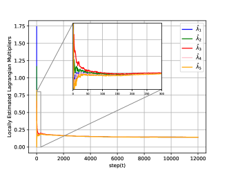
Figure 1: Convergence of locally estimated Lagrangian multipliers during training.

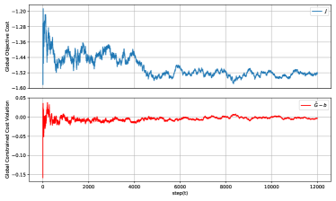
Figure 2: Global objective cost ($J$) and global constraint cost ($\hat{G}-b$) during training. The plot illustrates how the algorithm seeks to decrease the objective cost while maintaining constraint violations near zero.

6 Conclusion

This paper introduced a distributed approach for solving cooperative CMARL problems, allowing agents to minimize a global objective function while respecting shared constraints. By leveraging a decentralized primal-dual algorithm based on actor-critic method, our approach enables each agent to estimate Lagrangian multipliers locally, achieving consensus and ensuring convergence to an equilibrium. We validated the method through a constrained cooperative Cournot game with stochastic dynamics. The results highlight the potential of our method for scalable, decentralized solutions in real-world applications, such as smart grids and autonomous systems. Future work will explore adaptations for more complex environments and dynamic constraints.

References

• [1] D. Silver, A. Huang, C. J. Maddison, A. Guez, L. Sifre, G. Van Den Driessche, J. Schrittwieser, I. Antonoglou, V. Panneershelvam, M. Lanctot et al., “Mastering the game of go with deep neural networks and tree search,” Nature, vol. 529, no. 7587, pp. 484–489, 2016.
• [2] J. Kober, J. A. Bagnell, and J. Peters, “Reinforcement learning in robotics: A survey,” The International Journal of Robotics Research, vol. 32, no. 11, pp. 1238–1274, 2013.
• [3] T. Chu, J. Wang, L. Codecà, and Z. Li, “Multi-agent deep reinforcement learning for large-scale traffic signal control,” IEEE Transactions on Intelligent Transportation Systems, vol. 21, no. 3, pp. 1086–1095, 2020.
• [4] U. Pham, Q. Luu, and H. Tran, “Multi-agent reinforcement learning approach for hedging portfolio problem,” Soft Computing, vol. 25, no. 12, pp. 7877–7885, 2021.
• [5] M. Roesch, C. Linder, R. Zimmermann, A. Rudolf, A. Hohmann, and G. Reinhart, “Smart grid for industry using multi-agent reinforcement learning,” Applied Sciences, vol. 10, no. 19, p. 6900, 2020.
• [6] K. Zhang, Z. Yang, and T. Başar, “Multi-agent reinforcement learning: A selective overview of theories and algorithms,” Handbook of Reinforcement Learning and Control, 2021.
• [7] T. T. Nguyen, N. D. Nguyen, and S. Nahavandi, “Deep reinforcement learning for multiagent systems: A review of challenges, solutions, and applications,” IEEE transactions on cybernetics, vol. 50, no. 9, pp. 3826–3839, 2020.
• [8] A. Oroojlooy and D. Hajinezhad, “A review of cooperative multi-agent deep reinforcement learning,” Applied Intelligence, vol. 53, no. 11, pp. 13 677–13 722, 2023.
• [9] Y. Zhang and M. M. Zavlanos, “Cooperative multiagent reinforcement learning with partial observations,” IEEE Transactions on Automatic Control, vol. 69, no. 2, pp. 968–981, 2023.
• [10] L. Cassano, K. Yuan, and A. H. Sayed, “Multiagent fully decentralized value function learning with linear convergence rates,” IEEE Transactions on Automatic Control, vol. 66, no. 4, pp. 1497–1512, 2020.
• [11] K. Zhang, Z. Yang, H. Liu, T. Zhang, and T. Basar, “Fully decentralized multi-agent reinforcement learning with networked agents,” in Proceedings of the 35th International Conference on Machine Learning (ICML), vol. 80.   PMLR, 2018, pp. 5872–5881.
• [12] B. Yongacoglu, G. Arslan, and S. Yüksel, “Decentralized learning for optimality in stochastic dynamic teams and games with local control and global state information,” IEEE Transactions on Automatic Control, vol. 67, no. 10, pp. 5230–5245, 2021.
• [13] Q. Zhang, K. Dehghanpour, Z. Wang, F. Qiu, and D. Zhao, “Multi-agent safe policy learning for power management of networked microgrids,” IEEE Transactions on Smart Grid, vol. 12, no. 2, pp. 1048–1062, 2021.
• [14] S. He, Y. Wang, S. Han, S. Zou, and F. Miao, “A robust and constrained multi-agent reinforcement learning electric vehicle rebalancing method in amod systems,” in 2023 IEEE/RSJ International Conference on Intelligent Robots and Systems (IROS), 2023, pp. 5637–5644.
• [15] E. Altman and A. Shwartz, “Constrained markov games: Nash equilibria,” in Advances in Dynamic Games and Applications.   Springer, 2000, pp. 213–221.
• [16] S. Paternain, L. Chamon, M. Calvo-Fullana, and A. Ribeiro, “Constrained reinforcement learning has zero duality gap,” in Advances in Neural Information Processing Systems (NeurIPS), vol. 32, 2019.
• [17] S. Paternain, M. Calvo-Fullana, L. F. Chamon, and A. Ribeiro, “Safe policies for reinforcement learning via primal-dual methods,” IEEE Transactions on Automatic Control, vol. 68, no. 3, pp. 1321–1336, 2022.
• [18] Z. Chen, Y. Zhou, and H. Huang, “On the hardness of constrained cooperative multi-agent reinforcement learning,” in Proceedings of the 12th International Conference on Learning Representations (ICLR), 2024.
• [19] S. Bhatnagar and K. Lakshmanan, “An online actor-critic algorithm with function approximation for constrained markov decision processes,” Journal of Optimization Theory and Applications, vol. 153, pp. 688–708, 2012.
• [20] R. B. Diddigi, D. S. K. Reddy, P. KJ, and S. Bhatnagar, “Actor-critic algorithms for constrained multi-agent reinforcement learning,” in Proceedings of the 18th International Conference on Autonomous Agents and MultiAgent Systems, 2019, pp. 1931–1933.
• [21] S. Lu, K. Zhang, T. Chen, T. Başar, and L. Horesh, “Decentralized policy gradient descent ascent for safe multi-agent reinforcement learning,” in Proceedings of the AAAI Conference on Artificial Intelligence, vol. 35, no. 10, 2021, pp. 8767–8775.
• [22] Y. Zhao, Y. Yang, Z. Lu, W. Zhou, and H. Li, “Multi-agent first order constrained optimization in policy space,” in Advances in Neural Information Processing Systems (NeurIPS), vol. 36, 2023, pp. 39 189–39 211.
• [23] R. Hassan, K. S. Wadith, M. M. Rashid, and M. M. Khan, “Depaint: A decentralized safe multi-agent reinforcement learning algorithm considering peak and average constraints,” Applied Intelligence, pp. 1–17, 2024.
• [24] Z. Yang, H. Jin, R. Ding, H. You, G. Fan, X. Wang, and C. Zhou, “Decom: Decomposed policy for constrained cooperative multi-agent reinforcement learning,” in Proceedings of the AAAI Conference on Artificial Intelligence, vol. 37, no. 9, 2023, pp. 10 861–10 870.
• [25] D. Ying, Y. Zhang, Y. Ding, A. Koppel, and J. Lavaei, “Scalable primal-dual actor-critic method for safe multi-agent reinforcement learning with general utilities,” Advances in Neural Information Processing Systems (NeurIPS), vol. 36, 2024.
• [26] T.-H. Chang, A. Nedić, and A. Scaglione, “Distributed constrained optimization by consensus-based primal-dual perturbation method,” IEEE Transactions on Automatic Control, vol. 59, no. 6, pp. 1524–1538, 2014.
• [27] A. Nedic and A. Ozdaglar, “Distributed subgradient methods for multi-agent optimization,” IEEE Transactions on Automatic Control, vol. 54, no. 1, pp. 48–61, 2009.
• [28] R. S. Sutton, “Reinforcement learning: An introduction,” 2018.
• [29] H. J. Kushner and D. S. Clark, Stochastic Approximation Methods for Constrained and Unconstrained Systems.   Springer, 1978.
• [30] Y. Zhang and K. W. Ross, “On-policy deep reinforcement learning for the average-reward criterion,” in Proceedings of the 38th International Conference on Machine Learning (ICML), vol. 139.   PMLR, 2021, pp. 12 535–12 545.