A novel polyhedral scaled boundary finite element method solving three-dimensional heat conduction problems

Abstract

In this work, we derived the three-dimensional scaled boundary finite element formulation for thermal conduction problems. By introducing Wachspress shape functions, we proposed a novel polyhedral scaled boundary finite element method (PSBFEM) to address thermal conduction problems. The proposed method effectively addresses the challenges associated with complex geometries by integrating the polyhedral mesh and the octree mesh. The presented formulation handles both steady-state and transient thermal conduction analyses. Through a series of numerical examples, the accuracy and convergence of the proposed method were validated. The results demonstrate that mesh refinement leads to superior accuracy for the PSBFEM compared to the FEM. Moreover, Polyhedral elements provide an effective and efficient approach for complex simulations that substantially reduces computational costs.

[inst1]organization=College of Water Conservancy and Hydropower Engineering, Hohai University,city=Nanjing, postcode=210098, state=Jiangsu, country=China [inst2]organization=PowerChina Kunming Engineering Corporation Limited,city=Kunming, postcode=650051, state=Yunnan, country=China [inst3]organization=College of Water Conservancy, Yunnan Agricultural University China,city=Kunming, postcode=650201, state=Yunnan, country=China

Derived a semi-analytical formulation to solving heat conduction problems based on the SBFEM

Developed a novel polyhedral SBFEM framework incorporating Wachspress shape functions

Implemented the PSBFEM in ABAQUS UEL to solve both steady-state and transient heat conduction problems

Achieved superior accuracy with PSBFEM compared to FEM during mesh refinement

polyhedral elements provide an efficient solution for complex simulations by significantly reducing computational costs

1 Introduction

Heat conduction problems are prevalent in modern engineering applications, such as electronic device cooling [1], material processing [2], nuclear reactor design [3], and civil engineering [4]. Accurately and efficiently solving three-dimensional (3D) heat conduction problems is essential for optimizing designs and enhancing system performance. Experimentation has often been employed to study heat conduction phenomena [5, 6]. However, these experimental methods can be time-consuming and costly, and may not capture all the nuances of the system, particularly in geometrically intricate or dynamically varying scenarios. Moreover, although analytical methods [7, 8] have been used over the past decades, they are typically limited by the complexities of geometry and boundary conditions. Consequently, numerical methods, particularly the finite element method (FEM), have become indispensable for addressing complex heat conduction problems [9, 10].

In traditional three-dimensional (3D) FEM, tetrahedral and hexahedral elements are widely utilized. However, the accuracy and reliability of FEM solutions depend heavily on mesh quality. Tetrahedral elements allow for automated mesh generation but often result in lower accuracy, while hexahedral elements provide higher accuracy but require manual intervention during the mesh generation process, making it more time-consuming. To achieve precision in computational results, high-quality meshes are typically generated through complex and time-consuming re-meshing algorithms. According to Sandia National Laboratories, preprocessing steps such as mesh generation account for more than 80% of the total analysis time [11]. To alleviate the burden of preprocessing, researchers have explored various alternative methods, including the boundary element method (BEM) [12], isogeometric analysis (IGA) [13], meshfree methods [14], and physics-informed neural networks (PINNs) [15]. Each of these methods aims to address specific challenges posed by FEM, particularly in terms of geometric complexity and computational cost, yet they present their own limitations in practice.

For large-scale problems, employing a locally refined mesh in regions of interest has become a common strategy, as it provides higher accuracy in critical areas while reducing the overall computational load [16]. This approach has given rise to non-matching mesh techniques, which allow for tailored meshing strategies that apply finer meshes where needed and coarser meshes elsewhere [17, 18]. However, non-matching meshes introduce the challenge of handling hanging nodes—nodes that do not align with those in adjacent elements. Traditional FEM struggles with such nodes due to the disruption of continuity and compatibility conditions, which are essential for accurate solutions [19].

Several techniques have been developed to manage hanging nodes, including the Arlequin method [20], the mortar segment-to-segment method [21], multi-point constraint equations [22], and the polygonal finite element method (PFEM) [23, 24]. Among these, PFEM inherently addresses non-matching mesh problems by treating hanging nodes as part of the element discretization. However, PFEM’s reliance on a weak formulation in each discretization direction often results in reduced computational accuracy.

The scaled boundary finite element method (SBFEM) has emerged as a robust technique for handling hanging nodes in quadtree and octree meshes [25, 26]. SBFEM combines the strengths of both FEM and BEM into a semi-analytical approach. Discretization occurs only in the circumferential direction, while the radial direction retains a strong form of the governing equations. This hybrid approach allows for significant computational efficiency, making it well-suited for complex engineering applications [27]. SBFEM’s ability to handle irregular meshes and discontinuities while maintaining high precision has led to its widespread application in various fields [28, 29, 30].

Moreover, to enhance the SBFEM’s capability in handling complex geometries, researchers have introduced polygonal and polyhedral techniques. For two-dimensional problems, Ye et al. [29, 31] combined the standard SBFEM with a polygonal mesh technique to solve static and dynamic problems. Ooi et al. [32] proposed a novel scaled boundary polygonal formulation to model elasto-plastic material responses in structures. For three-dimensional problems, Ya et al. [33] extended the SBFEM to study interfacial problems using polyhedral meshes. Furthermore, Yang et al. [34] developed UEL and VUEL implementations in ABAQUS to perform static and elastodynamic stress analyses in solids. In these methods, boundary surfaces are discretized with quadrilateral and triangular elements, resulting in polyhedral elements that exhibit relatively complex topologies.

Recent studies have extended SBFEM to heat conduction problems. For instance, Bazyar et al. [35] used SBFEM to solve 2D heat conduction problems in anisotropic media. Yu et al. [36] applied a hybrid quadtree mesh in SBFEM to analyze transient heat conduction problems involving cracks or inclusions. Yang et al. [37] developed a user element (UEL) of polygonal SBFEM to solve 2D heat conduction problems. However, most current research focuses on 2D problems. For 3D heat conduction problems, Lu et al. [38] developed a modified SBFEM to address steady-state heat conduction problems, but transient analysis remains underexplored.

In this work, a novel polyhedral SBFEM framework is proposed for solving 3D steady-state and transient heat conduction problems. The remainder of this paper is organized as follows: Sections 2 and 3 derive the formulation of the SBFEM for 3D heat conduction analysis. Section 4 develops a novel polyhedral SBFEM by incorporating Wachspress shape functions. Section 5 presents the solution procedure for the SBFEM equations. Section 6 describes the implementation process for solving heat conduction problems using SBFEM in Abaqus UEL. Section 7 provides several numerical examples to demonstrate the accuracy and efficiency of the proposed method. Finally, Section 8 concludes the paper by summarizing the key findings.

2 Governing equations of the 3D heat conduction problems

We considered a 3D transient heat conduction problems, the governing equations without heat sources are written as

$$\rho c\dot{{T}}-\nabla\cdot(\mathbf{k}\nabla{T})=\mathbf{0}\quad\text{in }\quad\Omega,$$ (1)

where $\rho$ denotes the mass density. $c$ is the heat capacity, $T$ is the temperature, $\dot{T}$ is the temperature change rate, $\nabla$ is the gradient operator; $\mathbf{k}$ is the matrix of the thermal conductivity, $\mathbf{k}$ can be written as:

$$\mathbf{k}=\begin{bmatrix}k_{x}&0&0\\ 0&k_{y}&0\\ 0&0&k_{z}\end{bmatrix}.$$ (2)

The initial conditions can be written as follows:

$$T(x,y,z,t=0)=T_{0}(x,y,z)\quad\text{in }\quad\Omega.$$ (3)

And the boundary conditions can be expressed as:

$$T(x,y,z)=\bar{T}\quad\mathrm{on~{}}S_{1},$$ (4)

$$-k\frac{\partial T}{\partial n}=\overline{q}_{n}=\begin{cases}\quad q_{2}&\text{on}\quad S_{2}\\ h(T-T_{\infty})&\text{on}\quad S_{3}\end{cases},$$ (5)

where $\Omega$ denotes the computational domain, $n$ is outward normal vector to $\Omega$. $S$ is the boundary. In addition, $\overline{T}$ and $q_{2}$ are the prescribed boundary temperature and heat flux, respectively. $h$ is the convection heat transfer coefficient and $T_{\infty}$ is the ambient temperature.

Applying the Fourier transform to Eq. (1) yields the governing equation in the frequency domain as follows:

$$\mathbf{k}\Delta\tilde{T}=i\omega\rho c\tilde{T},$$ (6)

where $\tilde{T}$ is the Fourier transform of $T$. $\omega$ is the frequency. When $\omega=0$, the problem reduces to a steady-state heat conduction scenario.

3 Formulation of SBFEM for heat conduction problems

3.1 Scaled boundary transformation of the geometry

The scaled boundary coordinates is shown in Fig. 1. The Cartesian coordinates of a point $(\hat{x},\hat{y},\hat{z})$ within the volume sector $\mathrm{V}_{\mathrm{e}}$ can be defined by the scaled boundary coordinates $(\xi,\eta,\zeta)$ as [39, 27]

$$\hat{x}(\xi,\eta,\zeta)=\xi\hat{x}(\eta,\zeta)=\xi\mathbf{N}(\eta,\zeta)\mathbf{\hat{x}},$$ (7a)

$$\hat{y}(\xi,\eta,\zeta)=\xi\hat{y}(\eta,\zeta)=\xi\mathbf{N}(\eta,\zeta)\mathbf{\hat{y}},$$ (7b)

$$\hat{z}(\xi,\eta,\zeta)=\xi\hat{z}(\eta,\zeta)=\xi\mathbf{N}(\eta,\zeta)\mathbf{\hat{z}},$$ (7c)

where $\hat{x}$, $\hat{y}$ and $\hat{z}$ are the nodal coordinate vectors of the surface element $\mathrm{S_{e}}$ in Cartesian coordinates. $\mathbf{N}(\eta,\zeta)$ is the shape function vector

$$\mathbf{N}(\eta,\zeta)=[N_{1}(\eta,\zeta)\quad N_{2}(\eta,\zeta)\quad...\quad N_{n}(\eta,\zeta)],$$ (8)

where $N_{i}(\eta,\zeta)$ denote the shape functions and $n$ represents the total number of nodes in the polyhedron.

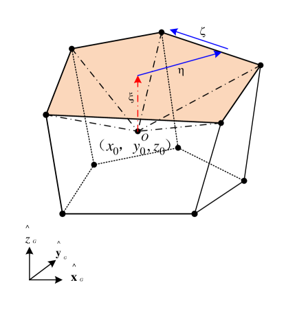
Figure 1: Scaled boundary coordinates ($\xi,\eta,\zeta$) represent the coordinate system centered at $O$, applicable to an arbitrary faceted polyhedron.

The partial derivatives with respect to the scaled boundary coordinates are related to those in Cartesian coordinates through the following equation:

$$\begin{Bmatrix}\frac{\partial}{\partial\xi}\\ \frac{\partial}{\partial\eta}\\ \frac{\partial}{\partial\zeta}\end{Bmatrix}=\begin{bmatrix}1&0&0\\ 0&\xi&0\\ 0&0&\xi\end{bmatrix}\mathbf{J_{b}}(\eta,\zeta)\begin{Bmatrix}\frac{\partial}{\partial x}\\ \frac{\partial}{\partial y}\\ \frac{\partial}{\partial z}\end{Bmatrix},$$ (9)

where $\mathbf{J_{b}}(\eta,\zeta)$ denotes the Jacobian matrix on the boundary $(\xi=1)$, and is defined as follows:

$$\mathbf{J_{b}}(\eta,\zeta)=\begin{bmatrix}\hat{x}(\eta,\zeta)&\hat{y}(\eta,\zeta)&\hat{z}(\eta,\zeta)\\ \hat{x}(\eta,\zeta)_{,\eta}&\hat{y}(\eta,\zeta)_{,\eta}&\hat{z}(\eta,\zeta)_{,\eta}\\ \hat{x}(\eta,\zeta)_{,\zeta}&\hat{y}(\eta,\zeta)_{,\zeta}&\hat{z}(\eta,\zeta)_{,\zeta}\end{bmatrix}.$$ (10)

The determinant of $\mathbf{J_{b}}(\eta,\zeta)$ is expressed as follows:

$$|\mathbf{J_{b}}|=\hat{x}(\hat{y}_{,\eta}\hat{z}_{,\zeta}-\hat{z}_{,\eta}\hat{y}_{,\zeta})+\hat{y}(\hat{z}_{,\eta}\hat{x}_{,\zeta}-\hat{x}_{,\eta}\hat{z}_{,\zeta})+\hat{z}(\hat{x}_{,\eta}\hat{y}_{,\zeta}-\hat{y}_{,\eta}\hat{x}_{,\zeta}),$$ (11)

where the argument $(\eta,\zeta)$ has been omitted for clarity. From Eq. (9), it can be inferred that the inverse relationship is given by:

$$\left\{\begin{array}[]{c}\frac{\partial}{\partial\hat{x}}\\ \frac{\partial}{\partial\hat{y}}\\ \frac{\partial}{\partial\hat{z}}\end{array}\right\}=\mathbf{J}^{-1}\left(\boldsymbol{\eta},\boldsymbol{\zeta}\right)\left\{\begin{array}[]{c}\frac{\partial}{\partial\xi}\\ \frac{1}{\xi}\frac{\partial}{\partial\eta}\\ \frac{1}{\xi}\frac{\partial}{\partial\zeta}\end{array}\right\},$$ (12)

where the inverse of the Jacobian matrix at the boundary, $\mathbf{J}^{-1}(\eta,\zeta)$, can be expressed as follows:

$$\left.\mathbf{J}^{-1}\left(\boldsymbol{\eta},\boldsymbol{\zeta}\right)=\frac{1}{\left|\mathbf{J}\right|}\left[\begin{array}[]{ccc}y_{,\boldsymbol{\eta}}z_{,\boldsymbol{\zeta}}-z_{,\boldsymbol{\eta}}y_{,\boldsymbol{\zeta}}&zy_{,\boldsymbol{\zeta}}-yz_{,\boldsymbol{\zeta}}&yz_{,\boldsymbol{\eta}}-zy_{,\boldsymbol{\eta}}\\ \\ z_{,\boldsymbol{\eta}}x_{,\boldsymbol{\zeta}}-x_{,\boldsymbol{\eta}}z_{,\boldsymbol{\zeta}}&xz_{,\boldsymbol{\zeta}}-zx_{,\boldsymbol{\zeta}}&zx_{,\boldsymbol{\eta}}-xz_{,\boldsymbol{\eta}}\\ \\ x_{,\boldsymbol{\eta}}y_{,\boldsymbol{\zeta}}-y_{,\boldsymbol{\eta}}x_{,\boldsymbol{\zeta}}&yx_{,\boldsymbol{\zeta}}-xy_{,\boldsymbol{\zeta}}&xy_{,\boldsymbol{\eta}}-yx_{,\boldsymbol{\eta}}\end{array}\right.\right].$$ (13)

Eq. (12) can also be expressed as

$$\left\{\begin{array}[]{c}\frac{\partial}{\partial\hat{x}}\\ \frac{\partial}{\partial\hat{y}}\\ \frac{\partial}{\partial\hat{z}}\end{array}\right\} =\frac{1}{|\mathbf{J}|}\left[\begin{array}[]{c}y_{,\eta}z_{,\zeta}-z_{,\eta}y_{,\zeta}\\ \\ z_{,\eta}x_{,\zeta}-x_{,\eta}z_{,\zeta}\\ \\ x_{,\eta}y_{,\zeta}-y_{,\eta}x_{,\zeta}\end{array}\right]\frac{\partial}{\partial\xi}$$ (14)

$$+\frac{1}{\xi}\left(\frac{1}{|\mathbf{J}|}\left[\begin{array}[]{c}zy_{,\zeta}-yz_{,\zeta}\\ \\ xz_{,\zeta}-zx_{,\zeta}\\ \\ yx_{,\zeta}-xy_{,\zeta}\end{array}\right]\frac{\partial}{\partial\eta}+\frac{1}{|\mathbf{J}|}\left[\begin{array}[]{c}yz_{,\eta}-zy_{,\eta}\\ \\ zx_{,\eta}-xz_{,\eta}\\ \\ xy_{,\eta}-yx_{,\eta}\end{array}\right]\frac{\partial}{\partial\zeta}\right).$$

The gradient operator in the Cartesian coordinate system can be transformed into the scaled boundary coordinate system as follows:

$$\nabla=\mathbf{b}_{1}\left(\eta,\zeta\right)\frac{\partial}{\partial\xi}+\frac{1}{\xi}\left(\mathbf{b}_{2}\left(\eta,\zeta\right)\frac{\partial}{\partial\eta}+\mathbf{b}_{3}\left(\eta,\zeta\right)\frac{\partial}{\partial\zeta}\right),$$ (15)

where $\mathbf{b}_{1}\left(\eta,\zeta\right)$, $\mathbf{b}_{2}\left(\eta,\zeta\right)$, and $\mathbf{b}_{3}\left(\eta,\zeta\right)$ can be defined as

$$\mathbf{b}_{1}\left(\eta,\zeta\right)=\left.\frac{1}{|\mathbf{J}|}\left[\begin{array}[]{c}y_{,\eta}z_{,\zeta}-z_{,\eta}y_{,\zeta}\\ \\ z_{,\eta}x_{,\zeta}-x_{,\eta}z_{,\zeta}\\ \\ x_{,\eta}y_{,\zeta}-y_{,\eta}x_{,\zeta}\end{array}\right.\right],$$ (16)

$$\mathbf{b}_{2}\left(\eta,\zeta\right)=\left.\frac{1}{|\mathbf{J}|}\left[\begin{array}[]{c}zy_{,\zeta}-yz_{,\zeta}\\ \\ xz_{,\zeta}-zx_{,\zeta}\\ \\ yx_{,\zeta}-xy_{,\zeta}\end{array}\right.\right],$$ (17)

$$\mathbf{b}_{3}\left(\eta,\zeta\right)=\left.\frac{1}{|\mathbf{J}|}\left[\begin{array}[]{c}yz_{,\eta}-zy_{,\eta}\\ \\ zx_{,\eta}-xz_{,\eta}\\ \\ xy_{,\eta}-yx_{,\eta}\end{array}\right.\right].$$ (18)

3.2 Temperature field

The temperature of any point $\tilde{T}(\xi,\eta,\zeta)$ in the SBFEM coordinates can be written as:

$$\tilde{T}(\xi,\eta,\zeta)=\mathbf{N}(\eta,\zeta)\tilde{T}(\xi),$$ (19)

where $\tilde{T}(\xi)$ is the nodal temperature vector and $\mathbf{N}(\eta,\zeta)$ is the matrix of shape function.

By using Eqs. (19) and (15), yields the temperature field partial derivatives as follows:

$$\begin{bmatrix}\frac{\partial\tilde{T}}{\partial\hat{x}}&\frac{\partial\tilde{T}}{\partial\hat{y}}&\frac{\partial\tilde{T}}{\partial\hat{z}}\end{bmatrix}^{\mathrm{\tilde{T}}}=\mathbf{b}_{1}\left(\boldsymbol{\eta},\boldsymbol{\zeta}\right)\frac{\partial\tilde{T}}{\partial\xi}+\frac{1}{\xi}\left(\mathbf{b}_{2}\left(\boldsymbol{\eta},\boldsymbol{\zeta}\right)\frac{\partial\tilde{T}}{\partial\boldsymbol{\eta}}+\mathbf{b}_{3}\left(\boldsymbol{\eta},\boldsymbol{\zeta}\right)\frac{\partial\tilde{T}}{\partial\boldsymbol{\zeta}}\right),$$ (20)

For the sake of simplicity, Eq. (20) can be rewritten by introducing the temperature expression in Eq. (19), as follows:

$$\begin{bmatrix}\frac{\partial\tilde{T}}{\partial\hat{x}}&\frac{\partial\tilde{T}}{\partial\hat{y}}&\frac{\partial\tilde{T}}{\partial\hat{z}}\end{bmatrix}^{\mathrm{\tilde{T}}}=\mathbf{B}_{1}\left(\eta,\zeta\right)\tilde{T}_{,\xi}+\frac{1}{\xi}\mathbf{B}_{2}\left(\eta,\zeta\right)\tilde{T},$$ (21)

where

$$\mathbf{B}_{1}\left(\eta,\zeta\right)=\mathbf{b}_{1}\left(\eta,\zeta\right)\mathbf{N}(\eta,\zeta),$$ (22)

$$\mathbf{B}_{2}\left(\eta,\zeta\right)=\mathbf{b}_{2}\left(\eta,\zeta\right)\mathbf{N}(\eta,\zeta)_{,\eta}+\mathbf{b}_{3}\left(\eta,\zeta\right)\mathbf{N}(\eta,\zeta)_{,\zeta}.$$ (23)

The heat flux $\tilde{Q}(\xi,\eta,\zeta)$ can be represented in the coordinate system of the SBFEM as follows:

$$\tilde{Q}(\xi,\eta)=-\mathbf{k}\Big{(}\mathbf{B_{1}}(\eta,\zeta)\tilde{T}(\xi)_{,\xi}+\frac{1}{\xi}\mathbf{B_{2}}(\eta,\zeta)\tilde{T}(\xi)\Big{)}.$$ (24)

3.3 Scaled boundary finite element equation

By employing Galerkin’s method, the scaled boundary finite element equation, expressed in terms of nodal temperature functions, is derived as follows:

$$\mathbf{E}_{0}\xi^{2}\tilde{T}(\xi)_{,\xi\xi}+\left(2\mathbf{E}_{0}-\mathbf{E}_{1}+\mathbf{E}_{1}^{T}\right)\xi\tilde{T}(\xi)_{,\xi}+\left(\mathbf{E}_{1}^{\mathrm{T}}-\mathbf{E}_{2}\right)\tilde{T}(\xi)-\mathbf{M}_{0}i\omega\xi^{2}\tilde{T}(\xi)=\xi\mathbf{F({\xi})}.$$ (25)

where coefficient matrices $\mathbf{E_{0}}$, $\mathbf{E_{1}}$, $\mathbf{E_{2}}$ and $\mathbf{M_{0}}$ of the entire element are assembled from the coefficient matrices $\mathbf{E_{0}^{e}}$, $\mathbf{E_{1}^{e}}$, $\mathbf{E_{2}^{e}}$ and $\mathbf{M_{0}^{e}}$ belonging to each surface element. The coefficient matrices $\mathbf{E_{0}^{e}}$, $\mathbf{E_{1}^{e}}$, $\mathbf{E_{2}^{e}}$, and $\mathbf{M_{0}^{e}}$ for a surface element $\mathrm{S_{e}}$ can be expressed as follows:

$$\mathbf{E}_{0}^{\mathrm{e}}=\int_{\mathbf{S}_{\mathrm{e}}}\mathbf{B}_{1}^{\mathrm{T}}\mathbf{kB}_{1}\left|\mathbf{J}_{\mathrm{b}}\right|\mathrm{d}\eta\mathrm{d}\zeta,$$ (26)

$$\mathbf{E}_{1}^{\mathrm{e}}=\int_{\mathbf{S}_{\mathrm{e}}}\mathbf{B}_{2}^{\mathrm{T}}\mathbf{kB}_{1}\left|\mathbf{J}_{\mathrm{b}}\right|\mathrm{d}\eta\mathrm{d}\zeta,$$ (27)

$$\mathbf{E}_{2}^{\mathrm{e}}=\int_{\mathrm{S}_{\mathrm{e}}}\mathbf{B}_{2}^{\mathrm{T}}\mathbf{kB}_{2}\left|\mathbf{J}_{\mathrm{b}}\right|\mathrm{d}\eta\mathrm{d}\zeta,$$ (28)

$$\mathbf{M_{0}^{e}}=\int_{\mathrm{S_{e}}}\mathbf{N^{T}}\rho\mathbf{N}\left|\mathbf{J_{b}}\right|\mathrm{d}\eta\mathrm{d}\zeta,$$ (29)

where $\rho$ is the mass density.

4 polyhedral SBFEM element

4.1 polyhedral element construction

In traditional 3D SBFEM, boundary surfaces are discretized using quadrilateral and triangular elements [33, 34]. As a result, the polyhedra processed by traditional 3D SBFEM exhibit relatively complex topologies, as illustrated in Fig. 2(a) and (c). The intricate topological geometry of such polyhedra is evident. To address this complexity, this work introduces polygonal discretization techniques that simplify the topological structure of the polyhedra, thereby reducing the number of element faces, as shown in Figs. 2(b) and (d). From the figures, it is clear that the polyhedra constructed using polygonal discretization significantly reduce the number of element faces, particularly for the octree mesh. This reduction not only enhances the efficiency of the mesh but also provides clearer visualization. Furthermore, Fig. 3 compares the traditional octree mesh with the polygon-based octree mesh surface, highlighting that the polygon-based octree mesh surface is more concise and has fewer faces.

To construct a novel polyhedral elements, we have introduced polygonal technology. As shown in Fig. 4, the polygonal surface of the polyhedron is first mapped onto a regular polygon. This regular polygon is then subdivided into smaller triangles, and each of these sub-triangles is subsequently mapped onto a standard triangle. Quadrature rules, commonly used in the FEM for numerical integration, are applied to these sub-triangles to perform the integration.

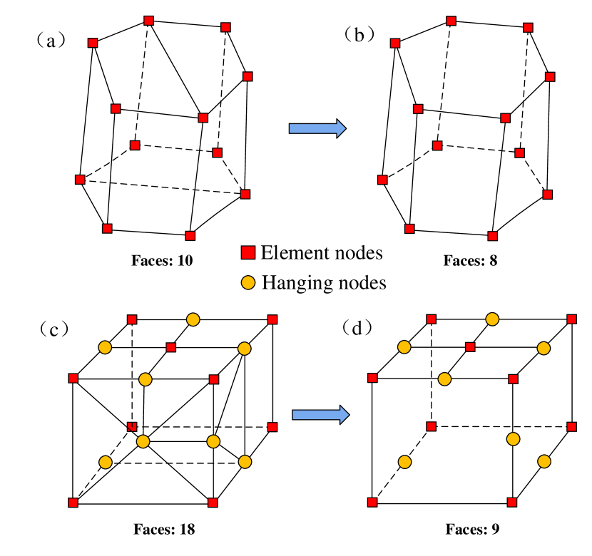
Figure 2: polyhedral elements construction based on polygonal surfaces: (a) traditional polyhedral element; (b) polyhedral element constructed from polygonal surfaces; (c) traditional octree element; (d) octree element constructed from polygonal surfaces.

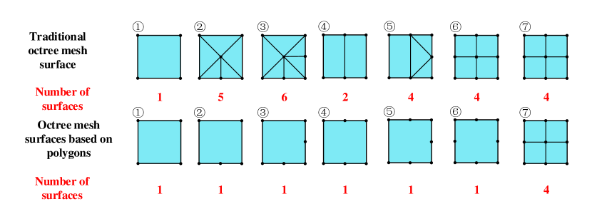
Figure 3: Comparison of the surfaces between traditional octree mesh and polygon-based octree mesh.

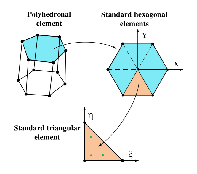
Figure 4: Numerical integration techniques for arbitrary polytopes.

4.2 Barycentric coordinates over polygonal surfaces

To effectively utilize these polygonal elements, we employ the Wachspress shape functions [40], which provide a systematic way to define the shape functions for polygonal elements. Wachspress introduced rational basis functions for polygonal elements using principles from projective geometry. These functions ensure nodal interpolation and maintain linearity along the boundaries by utilizing the algebraic equations of the edges. Warren [41, 42] extended Wachspress shape functions to simplex convex polyhedra. The construction of these coordinates is as follows: Let $R\subset\mathbb{P}^{3}$ be a simple convex polyhedron with facets $F$ and vertices $V$. For each facet $f\in F$, let $n_{f}$ represent the unit outward normal. For any point $x\in P$, let $h_{f}(x)$ denote the perpendicular distance from $x$ to the facet $f$, which is calculated as follows:

$$h_{f}(\mathbf{x})=(\mathbf{v}-\mathbf{x})\cdot\mathbf{n}_{f},$$ (30)

for any vertex $v\in V$ that belongs to a facet $f$, let $f_{1},f_{2},f_{3}$ be the three faces incident to $v$. For any point $x\in P$, let

$$w_{\mathbf{v}}(\mathbf{x})=\frac{\det(\mathbf{p}_{f_{1}},\mathbf{p}_{f_{2}},\mathbf{p}_{f_{3}})}{h_{f_{1}}(\mathbf{x})h_{f_{2}}(\mathbf{x})h_{f_{3}}(\mathbf{x})}.$$ (31)

where $\mathbf{p}_{f}(x)\equiv\frac{\mathbf{n}_{f}}{h_{f}(x)}$ is the scaled normal vector, and $f_{1},f_{2},\ldots,f_{d}$ are the $d$ faces adjacent to $v$, listed in counter-clockwise order around $v$ as viewed from outside $P$. The symbol $\det$ denotes the regular vector determinant in $\mathbb{R}^{d}$. The shape functions for $x\in P$ are then given by

$$\phi_{\mathbf{v}}(\mathbf{x})=\frac{w_{\mathbf{v}}(\mathbf{x})}{\sum_{\mathbf{u}\in V}w_{\mathbf{u}}(\mathbf{x})}.$$ (32)

Figure 5: Barycentric coordinates: Wachspress basis function.

5 Solution procedure

5.1 Stiffness matrix solution

The steady-state temperature field within the SBFEM formulation can be obtained by substituting $\omega$ into Eq. (25), yielding the following result:

$$\mathbf{E}_{0}\xi^{2}\tilde{\mathbf{T}}(\xi)_{,\xi\xi}+\left(2\mathbf{E}_{0}-\mathbf{E}_{1}+\mathbf{E}_{1}^{\mathrm{T}}\right)\xi\tilde{\mathbf{T}}(\xi)_{,\xi}+\left(\mathbf{E}_{1}^{\mathrm{T}}-\mathbf{E}_{2}\right)\tilde{\mathbf{T}}(\xi)=\mathbf{0}.$$ (33)

By introducing the variable,

$$\mathbf{X}(\xi)=\begin{bmatrix}\xi^{0.5}\tilde{\mathbf{h}}(\xi)\\ \xi^{-0.5}\tilde{\mathbf{Q}}(\xi)\end{bmatrix}.$$ (34)

The SBFEM equation can be transformed into a first-order ODE:

$$\xi\mathbf{X}(\xi)_{,\xi}=\mathbf{Z}_{\mathrm{p}}\mathbf{X}(\xi),$$ (35)

where the coefficient matrix $\mathbf{Z}_{\mathrm{p}}$ is a Hamiltonian matrix and defined as

$$\mathbf{Z_{p}}=\begin{bmatrix}-\mathbf{E}_{0}^{-1}\mathbf{E}_{1}^{\mathrm{T}}+0.5\mathbf{I}&\mathbf{E}_{0}^{-1}\\ \mathbf{E}_{2}-\mathbf{E}_{1}\mathbf{E}_{0}^{-1}\mathbf{E}_{1}^{\mathrm{T}}&\mathbf{E}_{1}\mathbf{E}_{0}^{-1}-0.5\mathbf{I}\end{bmatrix}.$$ (36)

The eigenvalue decomposition of $\mathbf{Z}_{\mathrm{p}}$ can be written as

$$\mathbf{Z}\begin{bmatrix}\mathbf{\Phi}_{\mathrm{h}}^{\mathrm{n}}&&\mathbf{\Phi}_{\mathrm{h}}^{\mathrm{p}}\\ \\ \mathbf{\Phi}_{\mathrm{q}}^{\mathrm{n}}&&\mathbf{\Phi}_{\mathrm{q}}^{\mathrm{p}}\end{bmatrix}=\begin{bmatrix}\mathbf{\Phi}_{\mathrm{h}}^{\mathrm{n}}&&\mathbf{\Phi}_{\mathrm{h}}^{\mathrm{p}}\\ \\ \mathbf{\Phi}_{\mathrm{q}}^{\mathrm{n}}&&\mathbf{\Phi}_{\mathrm{q}}^{\mathrm{p}}\end{bmatrix}\begin{bmatrix}\lambda^{\mathrm{n}}&&0\\ \\ 0&&\lambda^{\mathrm{p}}\end{bmatrix},$$ (37)

where $\mathbf{\Phi}_{h}^{n}$ and $\mathbf{\Phi}_{q}^{n}$ are the corresponding eigenvectors of $\lambda^{n}$, and $\mathbf{\Phi}_{h}^{p}$ and $\mathbf{\Phi}_{q}^{p}$ are the corresponding eigenvectors of $\lambda^{p}$. As a whole, $\mathbf{\Phi}_{h}$ and $\mathbf{\Phi}_{q}$ is the temperature and flux, respectively. The solution of equals

$$\mathbf{X}(\xi)=\begin{bmatrix}\mathbf{\Phi_{h}^{n}}&&\mathbf{\Phi_{h}^{p}}\\ \\ \mathbf{\Phi_{q}^{n}}&&\mathbf{\Phi_{q}^{p}}\end{bmatrix}\begin{bmatrix}\xi^{\lambda^{n}}&&\mathbf{0}\\ \\ \mathbf{0}&&\xi^{\lambda^{p}}\end{bmatrix}\begin{Bmatrix}\mathbf{c^{n}}\\ \\ \mathbf{c^{p}}\end{Bmatrix},$$ (38)

where the integration constants $\mathbf{c^{n}}$ and $\mathbf{c^{p}}$ are determined from the boundary conditions. The solution for $\mathbf{h}(\xi)$ and $\mathbf{q}(\xi)$ are

$$\mathbf{h}(\xi)=\mathbf{\Phi}_{\mathrm{h}}^{(\mathrm{n})}\xi^{-\lambda^{(\mathrm{n})}-0.5(s-2)\mathbf{I}}\mathbf{c}^{(\mathrm{n})},$$ (39)

$$\mathbf{q(\xi)=\Phi_{q}^{(n)}\xi^{-\lambda^{(n)}+0.5(s-2)I}c^{(n)}}.$$ (40)

The relationship between the nodal temperature functions and the nodal flux functions can be established by eliminating the integration constants as follows:

$$\mathbf{q}(\xi)=\Phi_{\mathbf{q}1}\Phi_{\mathbf{h}1}^{-1}\xi\mathbf{h}(\xi).$$ (41)

On the boundary $(\xi=1)$, the nodal flux vector $\mathbf{F}=\mathbf{q}(\xi=1)$ and the nodal temperature vector $\mathbf{d}=\mathbf{h}(\xi=1)$ apply. The relationship between nodal force and displacement vectors is $\mathbf{F}=\mathbf{K}\mathbf{d}$, therefore, the stiffness matrix of the subdomain is expressed as

$$\mathbf{K}=\mathbf{\Phi}_{\mathbf{q}1}\mathbf{\Phi}_{\mathbf{u}1}^{-1},$$ (42)

5.2 Mass matrix solution

The mass matrix of a volume element is formulated as

$$\mathbf{M}=\mathbf{\Phi}_{\mathrm{u}1}^{-\mathrm{T}}\int_{0}^{1}\xi^{\boldsymbol{\Lambda}^{+}}\mathbf{m}_{0}\xi^{\boldsymbol{\Lambda}^{+}}\xi\mathrm{d}\xi\boldsymbol{\Phi}_{\mathrm{u}1}^{-1},$$ (43)

where the coefficient matrix $\mathbf{m}_{0}$ is given by

$$\mathbf{m}_{0}=\Phi_{\mathbf{u}1}^{\mathrm{T}}\mathbf{M}_{0}\Phi_{\mathbf{u}1}.$$ (44)

By converting the integration component in Eq. (43) into matrix form, the expression for the mass matrix can be rewritten as follows:

$$\mathbf{M}=\Phi_{\mathrm{u}1}^{-\mathrm{T}}\mathbf{m}\Phi_{\mathrm{u}1}^{-1},$$ (45)

where

$$\mathbf{m}=\int_{0}^{1}\xi^{\boldsymbol{\Lambda}^{+}}\mathbf{m}_{0}\xi^{\boldsymbol{\Lambda}^{+}}\xi\mathrm{d}\xi.$$ (46)

Each entry of the matrix $\mathbf{m}$ can be evaluated analytically, yielding the following result:

$$m_{ij}=\frac{m_{0ij}}{\lambda_{ii}^{+}+\lambda_{jj}^{+}+2},$$ (47)

where $m_{0ij}$ is the entry of $m_{0}$ and $\lambda^{+}_{ii}$ and $\lambda^{+}_{ii}$ are particular entries of $\Lambda^{+}$.

5.3 Transient solution

The nodal temperature relationship for a bounded domain can be expressed as a standard time-domain equation, utilizing the steady-state stiffness and mass matrices, as follows:

$$\mathbf{K}\mathbf{T}(t)+\mathbf{M}\dot{\mathbf{T}}(t)=\mathbf{Q}(t),$$ (48)

where the nodal temperature $\mathbf{T}(t)$ is continuous derivative of time. Obtaining the functional solution in the time domain is challenging. In this work, the backward difference method [43] is employed to solve Eq. (48). The time domain is discretized into several time steps, and the solution at each time node is incrementally computed based on the initial conditions. The nodal water head at any given time is then determined through interpolation.

At time $\left[t,t+\Delta t\right]$, the temperature change rate $\dot{\mathbf{T}}(t)$ can be expressed as

$$\dot{\mathbf{T}}(t)=\frac{\Delta\mathbf{T}}{\Delta t}=\frac{\mathbf{T}(t)^{t+\Delta t}-\mathbf{T}(t)^{t}}{\Delta t}.$$ (49)

Eq. (49) is substituted into Eq. (48), and the equation at time step $t+\Delta t$ can be obtained as follows:

$$\mathbf{K}^{t+\Delta t}+\frac{\mathbf{M}^{t+\Delta t}}{\Delta t}\mathbf{T}(t)^{t+\Delta t}=\mathbf{Q}(t)^{t+\Delta t}+\frac{\mathbf{M}^{t+\Delta t}}{\Delta t}\mathbf{T}(t)^{t},$$ (50)

6 Implementation

6.1 Implementation of the UEL

Algorithm 1 provides a flowchart outlining the procedure for steady-state and transient heat conduction analysis, which has been successfully implemented in ABAQUS using the User Element (UEL) programming interface. The primary function of the UEL in ABAQUS is to update the element’s contribution to the residual force vector (RHS) and the stiffness matrix (AMATRX) via the user subroutine interface provided by the software. For steady-state heat conduction analysis, the AMATRX and the RHS are defined as follows:

$$\mathrm{AMATRX}=\mathbf{K},$$ (51)

$$\mathrm{RHS}=-\mathbf{K}\mathbf{U},$$ (52)

where $\mathbf{U}$ is the nodal temperature vector.

For the transient heat conduction, AMATRX and RHS are defined as follows:

$$\mathrm{AMATRX}=\mathbf{K}^{t+\Delta t}+\frac{\mathbf{M}^{t+\Delta t}}{\Delta t},$$ (53)

$$\mathrm{RHS}=-\mathbf{K}^{t+\Delta t}\mathbf{U}^{t+\Delta t}-\frac{\mathbf{M}^{t+\Delta t}}{\Delta t}\Big{(}\mathbf{U}^{t+\Delta t}-\mathbf{U}^{t}\Big{)}.$$ (54)

Additionally, it is necessary to construct the element geometry using nodal coordinates and node connectivity information. The element is first constructed to define the numbering and connectivity of the element nodes. As illustrated in Figs. 6(a) and (b), a hexahedral element and an octahedral element are considered. The numbering of the element faces is defined, followed by the connectivity information of the nodes on each face.

Algorithm 1 Solving the 3D heat conduction problems using the PSBFEM

Input: Node and element information, material properties, and nodal temperature $\mathbf{u}_{t}$
Output: Nodal temperature $\mathbf{u}_{t+1}$

1:while ABAQUS not converged do

2:     Solve nodal temperature $\mathbf{u}^{k}_{t+1}$

3:     for 1 to AllEle do   ! Traverse all elements

4:         Construct the geometry of elements

5:         Solve the the centre of elements

6:         Solve the coefficient matrices $\mathbf{E^{e}_{0}}$,$\mathbf{E^{e}_{1}}$,$\mathbf{E^{e}_{2}}$,and $\mathbf{M^{e}_{0}}$ using Eq. (26) $\sim$ Eq. (29)

7:         Construct $\mathbf{Z_{p}}$ using Eq. (36)

8:         Solve the $\mathbf{Z_{p}}$ by eigenvalue decomposition using Eq. (37)

9:         solve the stiffness $\mathbf{K}$ and mass matrix $\mathbf{M}$ using Eq. (42) and Eq. (46)

10:         if lflags(1)=31 then

11:              Update stiffness matrix $\mathbf{AMATRX}$ and residual force vetor $\mathbf{RHS}$ using Equations (51) and (52)

12:         end if

13:         if lflags(1)=32 or lflags(1)=33 then

14:              Update stiffness matrix $\mathbf{AMATRX}$ and residual force vetor $\mathbf{RHS}$ using Eqs. (52) and (54)

15:         end if

16:     end for

17:     update $k=k+1$

18:     Solve nodal temperature $\mathbf{u}_{t+1}$=$\mathbf{u}^{k}_{t+1}$

19:end while

6.2 Defining the element of the UEL

In 3D PSBFEM analysis, the geometry of elements is constructed based on the nodes. Fig. 6 illustrates an example of element construction. Prior to the analysis, it is necessary to establish the geometric relationships of the element’s surfaces according to their numbering, ensuring that the Jacobian matrix is negative. This requires that the direction of each surface points outward from the element. Fig. 7 shows the supported element types in the PSBFEM. In the PSBFEM, traditional elements such as tetrahedral, wedge, and hexahedral elements can be used. Additionally, the PSBFEM also provides more complex element types, including polyhedral and octree elements. Thus, the PSBFEM serves as an effective tool for solving complex geometries in numerical analysis.

The ABAQUS input file typically provides a comprehensive representation of the numerical model, detailing aspects such as nodes, elements, degrees of freedom, and materials. As shown in Listing 1, the hexahedral element (U8) is defined as follows: Lines 1 to 4 are used to define the pentagonal element (U8). Line 1 assigns the element type, number of nodes, number of element properties, and number of degrees of freedom for each node; Line 2 sets the active degrees of freedom for temperature; Lines 3 and 4 define the element set labeled Hexahedron. Similarly, other elements can be defined using the same method.

⬇

1[caption={Input file of the polyhedral element in UEL.}]

2*USER ELEMENT,NODES=8,TYPE=U8,PROPERTIES=5,COORDINATES=3,VARIABLES=8

311

4*Element,TYPE=U8,ELSET=Hexahedron

51, 5, 6, 8, 7, 1, 2, 4, 3

6*USER ELEMENT,NODES=12,TYPE=U12,PROPERTIES=5,COORDINATES=3,VARIABLES=12

711

8*Element,TYPE=U12,ELSET=Octahedron

92, 7, 8, 9, 10, 11, 12, 1, 2, 3, 4, 5, 6

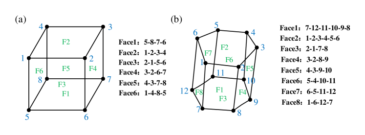
Figure 6: An example of face numbering for polyhedral elements: (a) hexahedral element; (b) polyhedral element.

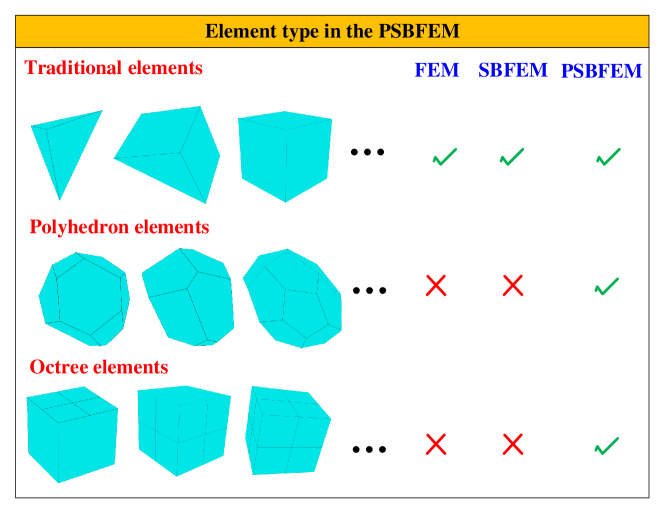
Figure 7: The supported elements of the PSBFEM.

7 Numerical examples

In this section, several benchmark problems are presented to demonstrate the convergence and accuracy of the proposed framework for heat conduction analysis. Moreover, the results obtained from the polyhedral SBFEM are compared with those from the FEM, with the FEM analysis performed using the commercial software ABAQUS. The comparisons were conducted on a system equipped with an Intel Core i7-4710MQ CPU (2.50 GHz) and 4.0 GB of RAM. To validate the proposed approach, the relative errors in temperature are examined as follows:

$$\mathbf{e}_{L_{2}}=\frac{\left\|\mathbf{T}_{num}-\mathbf{T}_{ref}\right\|_{L_{2}}}{\parallel\mathbf{T}_{ref}\parallel_{L_{2}}},$$ (55)

where $\mathbf{T}_{num}$ is the numerical result and $\mathbf{T}_{ref}$ is the reference solution.

7.1 Patch test

To verify that the proposed method satisfies the convergence requirement, it must pass the standard patch test [33, 44]. As shown in Fig. 8 a, the patch test is conducted using a quadrangular prism ($a=1$, $b=1$, $h=1$). The material constants are a thermal conductivity of 1.0 W/m/${}^{\circ}\mathrm{C}$ and a volumetric heat capacity of $\rho c=1.0\mathrm{J}/(\mathrm{m}^{3}\cdot^{\circ}\mathrm{C})$. Temperatures of $T=100^{\circ}\mathrm{C}$ and $T=0^{\circ}\mathrm{C}$ are prescribed on the top surface ($z=1$) and bottom surface ($z=0$), respectively. The temperature distribution is shown in Fig. 8(b). Tab. 1 presents the relative errors for nodal temperatures calculated at all nodes and compared to the analytical solution. The maximum relative error of the proposed method in temperature compared to the analytical solution is $1.53\times 10^{-4}$. Thus, the proposed method passes the patch test with sufficient accuracy.

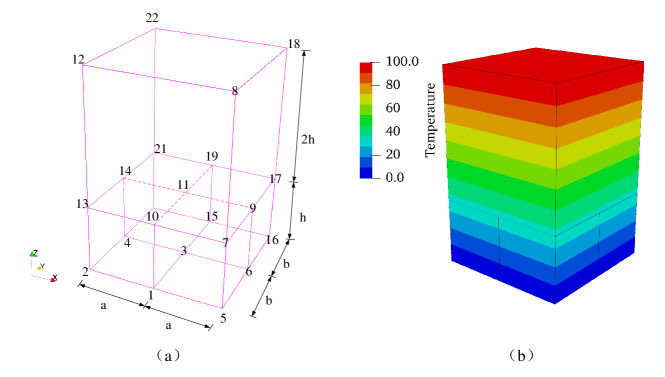
Figure 8: Geometry model and temperature contour of the patch test (Unit: ${}^{\circ}\mathrm{C}$).

Table 1: Maximum relative error of the nodal temperature.

Proposed method	Analytical solution	Relative error
33.3282	33.3333	$1.53\times 10^{-4}$

7.2 3D heat conduction beam

In this example, we examine a 3D heat conduction problem, as illustrated in Fig. 9. The beam has a length of 6 meters, with a width and height of 1.5 meters. A temperature of $T=70^{\circ}\mathrm{C}$ is applied at the left boundary ($z=0$), while a temperature of $T=30^{\circ}\mathrm{C}$ is imposed along the upper right boundary ($z=6\,\mathrm{m}$, $y=1.5\,\mathrm{m}$). The material has a thermal conductivity of 1.0 W/m/${}^{\circ}\mathrm{C}$ and a volumetric heat capacity of $\rho c=1.0\,\mathrm{J}/(\mathrm{m}^{3}\cdot^{\circ}\mathrm{C})$.

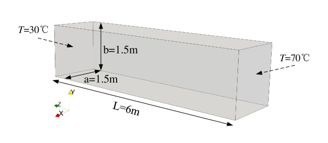
Figure 9: Geometry and boundary conditions for a 3D heat conduction beam.

The domain is discretized using hexahedral and polyhedral elements. A convergence study is conducted with both types of mesh. We refine the meshes successively following the sequence $h=1.0$, $0.5$, $0.25$, and $0.1\,\mathrm{m}$, as shown in Fig. 10. Moreover, Fig. 10(e) presents a cross-sectional view of a mesh layer along with several representative polyhedral elements. Fig. 11 shows that the PSBFEM and FEM exhibit a good convergence rate, with the accuracy of both methods increasing as the mesh is refined. When the mesh size was $0.1\,\mathrm{m}$, the relative errors for the FEM and PSBFEM were $2.1\times 10^{-4}$ and $5.5\times 10^{-5}$, respectively. The relative errors of the PSBFEM were smaller than those of the FEM for the same element size. Additionally, Fig. 12 demonstrates a significant concurrence in the temperature distribution between the PSBFEM and the analytical solution with refined meshes.

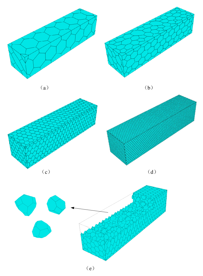
Figure 10: Four levels of polyhedral mesh refinement: (a) 1.0 m mesh size; (b) 0.5 m mesh size; (c) 0.25 m mesh size; (d) 0.1 m mesh size; (e) internal element of the 0.25 m mesh size.

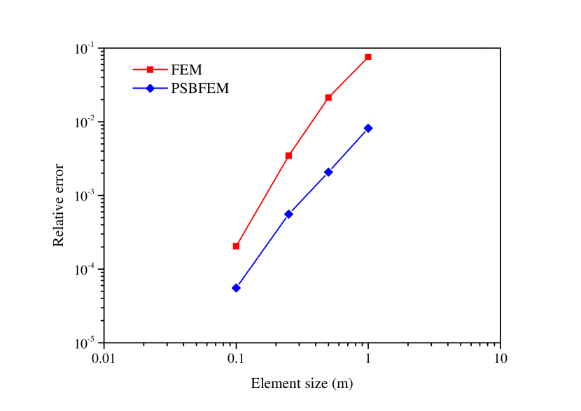
Figure 11: Convergence of the relative error in temperature.

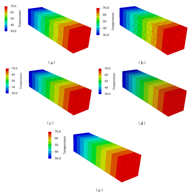
Figure 12: Temperature distribution of the 3D heat conduction beam using polyhedral mesh refinement: (a) 1.0 m mesh size; (b) 0.5 m mesh size; (c) 0.25 m mesh size; (d) 0.1 m mesh size; (e) analytical solution (Unit: ${}^{\circ}\mathrm{C}$).

To demonstrate the capability of octree mesh discretization in multi-scale analysis, we discretized a 3D heat conduction beam using an octree mesh, as shown in Fig. 13. Figs. 13(a) and 13 (b) represent the coarse and fine meshes, respectively, while Figs. 13(c) and 13(d) depict the multi-scale meshes. Additionally, Fig. 13(e) shows a cross-section of Multi-scale Mesh 2. Tab. LABEL:tab:ex01_t1 illustrates the mesh characteristics and relative errors for the multi-scale meshes. The relative errors for Multi-scale Mesh 2 and the fine mesh are both on the order of $10^{-4}$, demonstrating a high level of computational accuracy. However, the computational time for Multi-scale Mesh 2 is shorter than that of the fine mesh. Thus, through multi-scale modeling, refining the mesh in specific regions can yield more accurate results while reducing computational time.

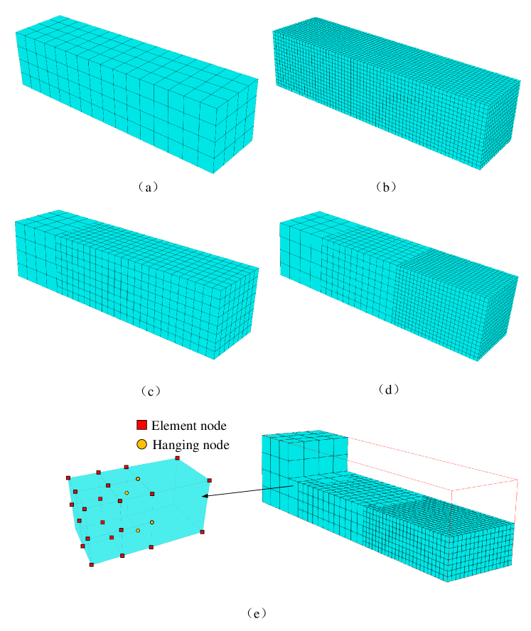
Figure 13: Multi-scale model of the 3D heat conduction beam using the octree mesh: (a) coarse mesh; (b) fine mesh; (c) multiscale mesh 1; (d) multi-scale mesh 2; (e) internal element of multi-scale mesh 2.

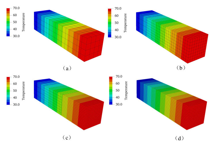
Figure 14: Temperature distribution of the 3D conduction beam using the octree mesh: (a) temperature contour with coarse mesh; (b) temperature contour with multi-scale mesh 1; (c) temperature contour with multi-scale mesh 2; (d) temperature contour with fine mesh; (Unit: ${}^{\circ}\mathrm{C}$).

Table 2: Mesh characteristics and relative errors for the multi-scale meshes.

Mesh type	Elements	Nodes	Faces	Relative error	CPU time (s)
Coarse mesh	256	425	1536	1.78$\times 10^{-2}$	0.20
Fine mesh	8432	12141	53328	6.33$\times 10^{-4}$	9.20
Multi-scale mesh 1	1572	2108	9504	2.80$\times 10^{-3}$	1.50
Multi-scale mesh 2	6696	8063	40512	8.49$\times 10^{-4}$	6.20

7.3 Steady-state heat conduction

In this example, we consider a classical steady-state heat conduction problem, as shown in Fig. 15. The length, width, and height of the cube are all 1 meter. The material has a thermal conductivity of 1.0 W/m/${}^{\circ}\mathrm{C}$ and a volumetric heat capacity of $\rho c=1.0\,\mathrm{J}/(\mathrm{m}^{3}\cdot^{\circ}\mathrm{C})$. The boundary conditions of the cube are shown in Eq. (56).

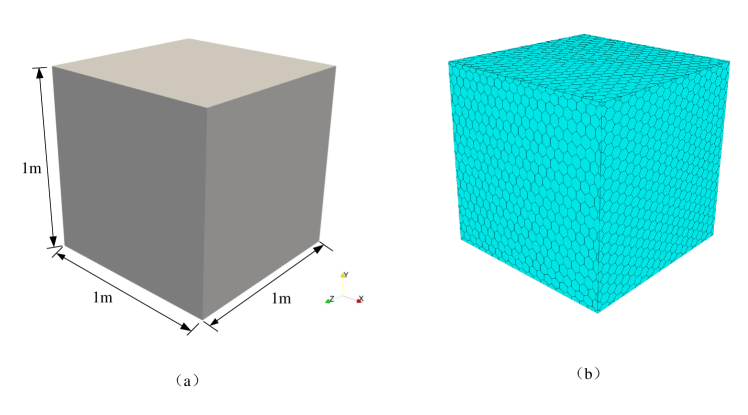
Figure 15: A cube for the steady-state heat conduction problem: (a) the geometry model; (b) the mesh with a size of 0.05 m.

$$(x,y,z)\in plane\perp(x=0),\quad T=0$$ (56)

$$(x,y,z)\in plane\perp(y=0),\quad T=0$$

$$(x,y,z)\in plane\perp(z=0),\quad T=0$$

$$(x,y,z)\in plane\perp(x=1),\quad T=0$$

$$(x,y,z)\in plane\perp(y=1),\quad T=\sin(\pi x)\sin(\pi z)$$

$$(x,y,z)\in plane\perp(z=1),\quad T=0$$

A convergence study was performed using mesh h-refinement, with successive refinements applied to mesh element sizes of 0.25 m, 0.1 m, 0.05 m, and 0.025 m. Fig. 15 b presents the polyhedral mesh with an element size of 0.05 m. The analytical solution for the temperature at point P ($x,y,z$) within the domain is calculated based on the approach outlined in [45]:

$$T(x,y,z)=\frac{\sinh(\pi y)}{\sinh(\pi)}\sin(\pi x)\sin(\pi z)$$ (57)

The convergence of the relative error in temperature with mesh refinement is presented in Fig. 16. It is observed that the PSBFEM converges to the analytical solution at an optimal rate. Furthermore, PSBFEM produces slightly more accurate results than FEM for the same element size. Fig. 17 illustrates the temperature distribution for both FEM and PSBFEM, showing that the results of both methods closely match the analytical solution.

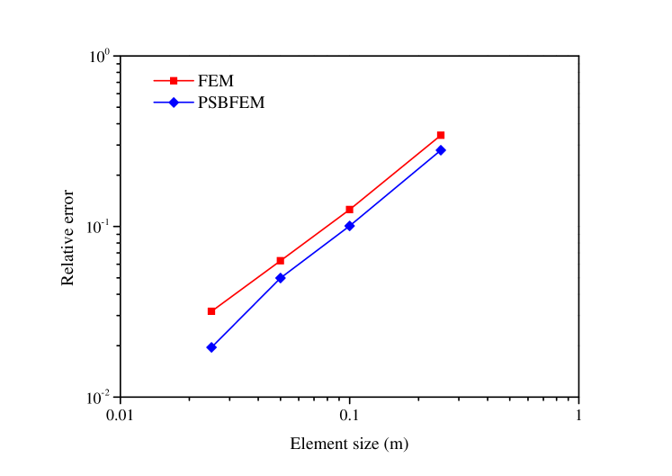
Figure 16: Convergence of the relative error in temperature.

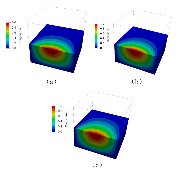
Figure 17: Temperature distribution of a cube for the steady-state heat conduction problem: (a) FEM; (b) PSBFEM; (c) analytical solution; (Unit: ${}^{\circ}\mathrm{C}$).

7.4 Transient heat conduction

To validate the proposed PSBFEM for the transient heat conduction problem in three dimensions, we examine a cubic domain $(\pi\times\pi\times\pi)$ with an analytical solution. The initial temperature distribution is defined as $T_{0}=10\sin(x)\sin(y)\sin(z)$. Homogeneous Dirichlet boundary conditions are applied on all surfaces of the cube, assuming a constant temperature of zero. The thermal properties of the material are given by a thermal conductivity $k=1.0\,\mathrm{W/m/^{\circ}\mathrm{C}}$ and a volumetric heat capacity $\rho c=1.0\,\mathrm{J}/(\mathrm{m}^{3}\cdot^{\circ}\mathrm{C})$. The corresponding analytical solution for the temperature field is expressed as [46]:

$$T(x,y,z,t)=10e^{-3t}\sin(x)\sin(y)\sin(z)$$ (58)

In both the PSBFEM and FEM simulations, a time step of $\Delta t=0.01\,\mathrm{s}$ was employed, with the total simulation time set to $t=1\,\mathrm{s}$. The computational domain was discretized using hexahedral and polyhedral elements. To assess the accuracy and convergence of the method, a convergence study was conducted through progressive mesh refinement.

The comparison of the convergence rates is presented in Fig. 18. It is observed that the convergence rates of PSBFEM and ABAQUS are identical. At the same element size, the accuracy of PSBFEM exceeds that of FEM. The temperature-time history at the monitoring point, obtained using FEM and PSBFEM, is compared in Fig. 19, where both methods show a good correspondence with the analytical solution. Furthermore, Fig. 20 illustrates the temperature distribution at different time steps for both PSBFEM and FEM. The results of both methods are in excellent agreement with the analytical solution.

Figure 18: Convergence of the relative error in temperature at different times: (a) $T=0.5\,\mathrm{s}$; (b) $T=1.0\,\mathrm{s}$.

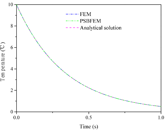
Figure 19: Comparison of the temperature time history at the monitoring point.

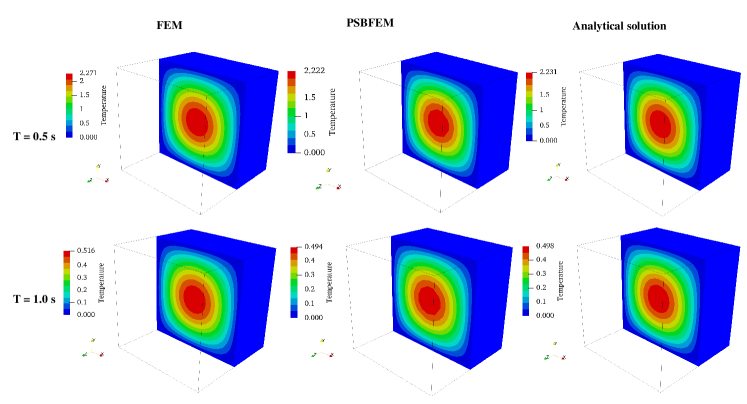
Figure 20: Distribution of the temperature for the two methods at different times; (Units:${}^{\circ}\mathrm{C}$)

7.5 Complex geometry analysis

With the rapid advancement of 3D printing, rapid prototyping, and digital analysis, the adoption of the STL format in finite element mesh generation has become increasingly essential. The simplicity and compatibility of the STL format allow efficient representation of complex three-dimensional geometries. In this study, polygonal meshes and octree-based meshes are utilized to automatically partition STL models, demonstrating the capability of PSBFEM to handle arbitrarily complex polygonal elements.

7.5.1 Stanford’s bunny using the polyhedral mesh

In this example, a Stanford bunny [47] given in STL format is used with a polyhedral mesh [48], as shown in Fig. 21(b). To further highlight the advantages of the polyhedral mesh, the model is also discretized using an unstructured tetrahedral mesh, as shown in Fig. 21(c). The material properties are as follows: thermal conductivity of 52 $\mathrm{W/m/^{\circ}C}$, specific heat of 434 $\mathrm{J/kg/^{\circ}C}$, and density of 7800 $\mathrm{kg/m^{3}}$. A temperature of $T=1000^{\circ}\mathrm{C}$ is prescribed on the bottom of the model, while an initial temperature of $T_{0}=20^{\circ}\mathrm{C}$ is applied throughout the entire model.

Tab. 3 presents a comparison between polyhedral and tetrahedral meshes based on several key metrics, including the number of nodes, elements, and surfaces. When using the same element size, the polyhedral mesh consists of 40,714 nodes, whereas the tetrahedral mesh contains only 7,132 nodes. Hence, the polyhedral mesh has a greater number of nodes at the same element size. Additionally, the polyhedral mesh requires only 132.60 seconds of CPU time, compared to the significantly higher 565.20 seconds required by the tetrahedral mesh. This suggests that polyhedral meshes could be a more effective choice for complex simulations, offering reduced computational costs. Furthermore, Fig. 22 illustrates that the temperature distributions for Stanford’s bunny using the two different element types exhibit remarkable agreement.

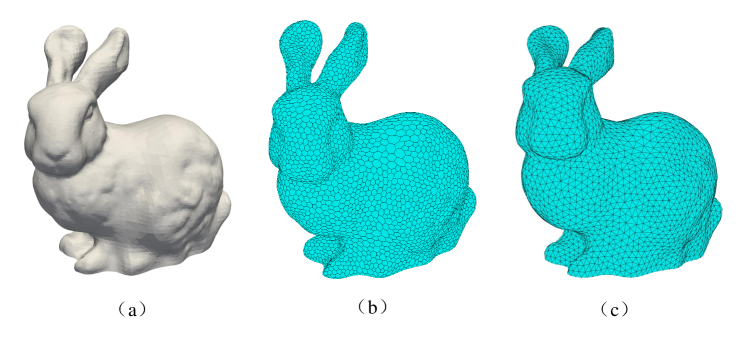
Figure 21: Geometry and mesh model of Stanford’s bunny; (a) the geometry model; (b) the polyhedral mesh; (c) the tetrahedral mesh.

Table 3: Mesh characteristics and relative errors of polyhedral and tetrahedral meshes.

Element type	Nodes	Elements	Surfaces	CPU time (s)
Polyhedron mesh	40714	7202	91879	132.60
Tetrahedral mesh	7132	32923	131692	565.20

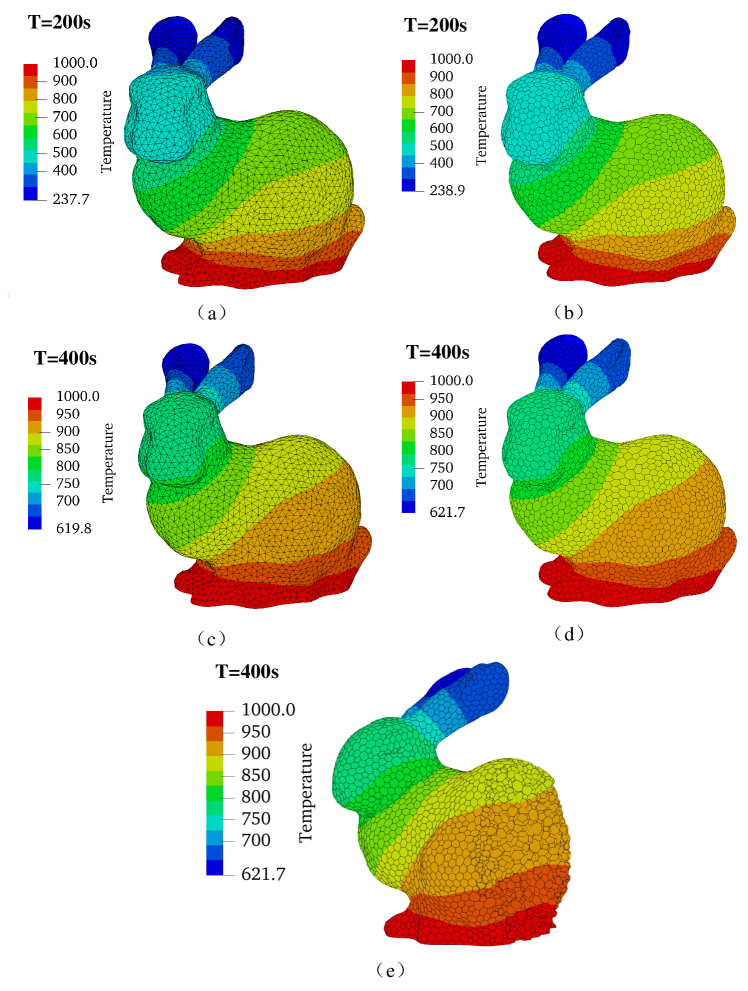
Figure 22: Temperature distribution of Stanford’s bunny using the PSBFEM: (a) temperature contour with tetrahedral elements at 200s; (b) temperature contour with polyhedral elements at 200s; (c) temperature contour with tetrahedral elements at 400s; (d) temperature contour with polyhedral elements at 400s; (e) localized contour of selected polyhedral elements from (d) at 400s.

7.5.2 Stanford’s luck using the hybrid octree mesh

The hybrid octree mesh is a mesh generation method that combines hexahedral (cubic) elements with other types of elements, such as tetrahedra and polyhedra. For more detailed information, please refer to the relevant literature [49]. In this example, Stanford’s bunny [47] is used with the hybrid octree mesh algorithm, as shown in Fig. 23(b). The cross-section of the hybrid octree mesh is illustrated in Fig. 24, which shows that the interior of the model is partitioned using a cubic octree mesh, while the outer boundary is formed by generating hybrid elements through a cutting process.

Tab. 4 presents the composition of the hybrid octree mesh. The mesh is made up of 68.7% octree elements and 31.3% hybrid elements. Since the majority of the mesh consists of high-quality cubic elements, the hybrid octree mesh achieves a high level of accuracy.

Moreover, Tab. 4 provides a comparison between the hybrid octree mesh and the tetrahedral mesh. The hybrid octree mesh contains more nodes but fewer elements and surfaces compared to the tetrahedral mesh. Additionally, the computational cost of the hybrid octree mesh is significantly lower than that of the tetrahedral mesh. Fig. 25 shows the temperature distribution for Stanford’s bunny using both mesh types, demonstrating a high degree of agreement between the results.

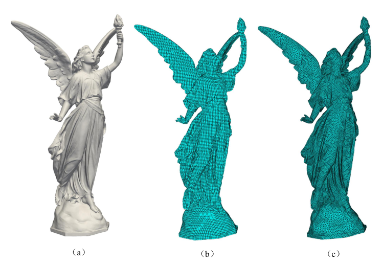
Figure 23: Geometry and mesh model of Stanford’s luck: (a) the geometry model; (b) the hybrid octree mesh; (c) the tetrahedral mesh.

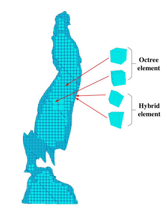
Figure 24: Cross-section view of the hybrid octree mesh for Stanford’s luck.

Table 4: Composition of hybrid octree mesh for the Stanford’s luck.

Element type	octree mesh	hybrid mesh
Number of elements	32939	15020
Proportion	68.7%	31.3%

Table 5: Mesh characteristics and relative errors of hybrid octree and tetrahedral meshes.

Element type	Nodes	Elements	Surfaces	CPU time (s)
Hybrid octree mesh	60579	47959	293594	209.60
Tetrahedral mesh	48684	222210	888840	859.40

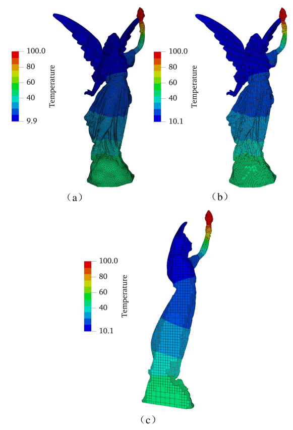
Figure 25: Temperature distribution of Stanford’s luck.

8 Conclusions

This paper presents a novel polyhedral SBFEM framework that demonstrates considerable advantages in solving three-dimensional steady-state and transient heat conduction problems. The key findings of this work are summarized as follows:

(1) By introducing polyhedral elements and utilizing Wachspress shape functions, the proposed method improves mesh efficiency, allowing for accurate solutions with fewer computational elements. This approach reduces preprocessing time, especially for complex geometries where traditional FEM methods would require extensive re-meshing.

(2) Numerical results demonstrate that the polyhedral SBFEM can achieve high accuracy, even with coarse meshes. In particular, the method outperforms traditional FEM in terms of convergence rates, with lower relative errors observed in both steady-state and transient heat conduction problems.

(3) The method’s ability to handle complex geometrical models, such as the Stanford Bunny, further highlights its versatility. Compared to hexahedral mesh, polyhedral meshes not only provide better accuracy but also significantly reduce computational times, showcasing the potential of this method for large-scale industrial applications.

(4) The hybrid octree mesh structure, in combination with SBFEM, enables efficient multi-scale analysis. This approach offers a balance between accuracy and computational cost, making it suitable for applications requiring high-resolution analysis in localized regions while maintaining global solution stability.

Future work could explore extending this framework to other types of physical problems, including thermal stress and multiphysics scenarios. Moreover, implementing adaptive meshing strategies within the polyhedral SBFEM framework could further enhance its applicability to real-time engineering simulations.

9 Acknowledgements

The National Natural Science Foundation of China (grant NO. 42167046), the Yunnan Province Xing Dian Talent Support Program (grant NO. XDYC-QNRC-2022-0764) and Yunan Funndamental Research Projects (grant NO. 202401CF070043) provided support for this study.

References

- [1] Z. Zhang, X. Wang, Y. Yan, A review of the state-of-the-art in electronic cooling, e-Prime-Advances in Electrical Engineering, Electronics and Energy 1 (2021) 100009.
- [2] S. P. Murzin, N. L. Kazanskiy, C. Stiglbrunner, Analysis of the Advantages of Laser Processing of Aerospace Materials Using Diffractive Optics, Metals 11 (6) (2021) 963. doi:10.3390/met11060963.
- [3] Z. Tian, X. Liu, C. Wang, D. Zhang, W. Tian, S. Qiu, G. Su, Experimental investigation on the heat transfer performance of high-temperature potassium heat pipe for nuclear reactor, Nuclear Engineering and Design 378 (2021) 111182.
- [4] L. D. Hung Anh, Z. Pásztory, An overview of factors influencing thermal conductivity of building insulation materials, Journal of Building Engineering 44 (2021) 102604. doi:10.1016/j.jobe.2021.102604.
- [5] C. Shi, Y. Wang, C. Xu, Experimental study and analysis on heat transfer coefficient of radial heat pipe, Journal of Thermal Science 19 (5) (2010) 425–429. doi:10.1007/s11630-010-0404-y.
- [6] S. Yang, J. Wang, G. Dai, F. Yang, J. Huang, Controlling macroscopic heat transfer with thermal metamaterials: Theory, experiment and application, Physics Reports 908 (2021) 1–65. doi:10.1016/j.physrep.2020.12.006.
- [7] W. Pophillat, G. Attard, P. Bayer, J. Hecht-Méndez, P. Blum, Analytical solutions for predicting thermal plumes of groundwater heat pump systems, Renewable Energy 147 (2020) 2696–2707. doi:10.1016/j.renene.2018.07.148.
- [8] A. Hobiny, I. Abbas, Analytical solutions of fractional bioheat model in a spherical tissue, Mechanics Based Design of Structures and Machines 49 (3) (2021) 430–439. doi:10.1080/15397734.2019.1702055.
- [9] M. Malek, N. Izem, M. Seaid, et al., A three-dimensional enriched finite element method for nonlinear transient heat transfer in functionally graded materials, International Journal of Heat and Mass Transfer 155 (2020) 119804.
- [10] S. Bilal, R. Mahmood, A. Majeed, I. Khan, K. S. Nisar, Finite element method visualization about heat transfer analysis of newtonian material in triangular cavity with square cylinder, Journal of Materials Research and Technology 9 (3) (2020) 4904–4918.
- [11] J. A. Cottrell, T. J. Hughes, Y. Bazilevs, Isogeometric analysis: toward integration of CAD and FEA, John Wiley & Sons, 2009.
- [12] E. Majchrzak, B. Mochnacki, The bem application for numerical solution of non-steady and nonlinear thermal diffusion problems, Computer Assisted Methods in Engineering and Science 3 (4) (2023) 327–346.
- [13] T. Yu, B. Chen, S. Natarajan, T. Q. Bui, A locally refined adaptive isogeometric analysis for steady-state heat conduction problems, Engineering Analysis with Boundary Elements 117 (2020) 119–131.
- [14] M. Afrasiabi, M. Roethlin, K. Wegener, Contemporary meshfree methods for three dimensional heat conduction problems, Archives of Computational Methods in Engineering 27 (2020) 1413–1447.
- [15] S. Cai, Z. Wang, S. Wang, P. Perdikaris, G. E. Karniadakis, Physics-informed neural networks for heat transfer problems, Journal of Heat Transfer 143 (6) (2021) 060801.
- [16] S. Li, X. Cui, N-sided polygonal smoothed finite element method (nsfem) with non-matching meshes and their applications for brittle fracture problems, Computer Methods in Applied Mechanics and Engineering 359 (2020) 112672.
- [17] M. Lacroix, S. Février, E. Fernández, L. Papeleux, R. Boman, J.-P. Ponthot, A comparative study of interpolation algorithms on non-matching meshes for pfem-fem fluid-structure interactions, Computers & Mathematics with Applications 155 (2024) 51–65.
- [18] B. V. Damirchi, M. R. Carvalho, L. A. Bitencourt Jr, O. L. Manzoli, D. Dias-da Costa, Transverse and longitudinal fluid flow modelling in fractured porous media with non-matching meshes, International Journal for Numerical and Analytical Methods in Geomechanics 45 (1) (2021) 83–107.
- [19] E. Ooi, H. Man, S. Natarajan, C. Song, Adaptation of quadtree meshes in the scaled boundary finite element method for crack propagation modelling, Engineering Fracture Mechanics 144 (2015) 101–117.
- [20] W. Sun, Z. Cai, J. Choo, Mixed arlequin method for multiscale poromechanics problems, International Journal for Numerical Methods in Engineering 111 (7) (2017) 624–659.
- [21] M. Zhou, B. Zhang, T. Chen, C. Peng, H. Fang, A three-field dual mortar method for elastic problems with nonconforming mesh, Computer Methods in Applied Mechanics and Engineering 362 (2020) 112870.
- [22] L. Jendele, J. Červenka, On the solution of multi-point constraints–application to fe analysis of reinforced concrete structures, Computers & Structures 87 (15-16) (2009) 970–980.
- [23] S. Biabanaki, A. Khoei, A polygonal finite element method for modeling arbitrary interfaces in large deformation problems, Computational Mechanics 50 (2012) 19–33.
- [24] H. Chi, C. Talischi, O. Lopez-Pamies, G. H. Paulino, Polygonal finite elements for finite elasticity, International Journal for Numerical Methods in Engineering 101 (4) (2015) 305–328.
- [25] H. Gravenkamp, A. A. Saputra, C. Song, C. Birk, Efficient wave propagation simulation on quadtree meshes using sbfem with reduced modal basis, International Journal for Numerical Methods in Engineering 110 (12) (2017) 1119–1141.
- [26] Y. Yang, Z. Zhang, Y. Feng, K. Wang, A novel solution for seepage problems implemented in the abaqus uel based on the polygonal scaled boundary finite element method, Geofluids 2022 (1) (2022) 5797014.
- [27] C. Song, The scaled boundary finite element method: introduction to theory and implementation, John Wiley & Sons, 2018.
- [28] C. Song, E. T. Ooi, S. Natarajan, A review of the scaled boundary finite element method for two-dimensional linear elastic fracture mechanics, Engineering Fracture Mechanics 187 (2018) 45–73.
- [29] N. Ye, C. Su, Y. Yang, Free and forced vibration analysis in abaqus based on the polygonal scaled boundary finite element method, Advances in Civil Engineering 2021 (1) (2021) 7664870.
- [30] K. Chen, D. Zou, X. Kong, X. Yu, An efficient nonlinear octree sbfem and its application to complicated geotechnical structures, Computers and Geotechnics 96 (2018) 226–245.
- [31] N. Ye, C. Su, Y. Yang, PSBFEM-Abaqus: Development of User Element Subroutine (UEL) for Polygonal Scaled Boundary Finite Element Method in Abaqus, Mathematical Problems in Engineering 2021 (2021) 1–22. doi:10.1155/2021/6628837.
- [32] E. T. Ooi, C. Song, F. Tin-Loi, A scaled boundary polygon formulation for elasto-plastic analyses, Computer Methods in Applied Mechanics and Engineering 268 (2014) 905–937. doi:10.1016/j.cma.2013.10.021.
- [33] S. Ya, S. Eisenträger, C. Song, J. Li, An open-source ABAQUS implementation of the scaled boundary finite element method to study interfacial problems using polyhedral meshes, Computer Methods in Applied Mechanics and Engineering 381 (2021) 113766. doi:10.1016/j.cma.2021.113766.
- [34] Z. Yang, F. Yao, Y. Huang, Development of ABAQUS UEL/VUEL subroutines for scaled boundary finite element method for general static and dynamic stress analyses, Engineering Analysis with Boundary Elements 114 (2020) 58–73. doi:10.1016/j.enganabound.2020.02.004.
- [35] M. H. Bazyar, A. Talebi, Scaled boundary finite-element method for solving non-homogeneous anisotropic heat conduction problems, Applied Mathematical Modelling 39 (23-24) (2015) 7583–7599.
- [36] B. Yu, P. Hu, A. A. Saputra, Y. Gu, The scaled boundary finite element method based on the hybrid quadtree mesh for solving transient heat conduction problems, Applied Mathematical Modelling 89 (2021) 541–571.
- [37] Y. Yang, Z. Zhang, Y. Feng, Y. Yu, K. Wang, L. Liang, A polygonal scaled boundary finite element method for solving heat conduction problems, arXiv preprint arXiv:2106.12283 (2021).
- [38] S. Lu, J. Liu, G. Lin, P. Zhang, Modified scaled boundary finite element analysis of 3d steady-state heat conduction in anisotropic layered media, International Journal of Heat and Mass Transfer 108 (2017) 2462–2471.
- [39] C. Song, A matrix function solution for the scaled boundary finite-element equation in statics, Computer Methods in Applied Mechanics and Engineering 193 (23-26) (2004) 2325–2356.
- [40] E. L. Wachspress, A rational basis for function approximation, in: Conference on Applications of Numerical Analysis: Held in Dundee/Scotland, March 23–26, 1971, Springer, 2006, pp. 223–252.
- [41] J. Warren, On the uniqueness of barycentric coordinates, Contemporary Mathematics 334 (2003) 93–100.
- [42] J. Warren, S. Schaefer, A. N. Hirani, M. Desbrun, Barycentric coordinates for convex sets, Advances in computational mathematics 27 (2007) 319–338.
- [43] O. Zienkiewicz, R. Taylor, O. Zienkiewicz, R. Taylor, The finite element method, vol. 1 mcgraw-hill (1989).
- [44] J. Zhang, S. Chauhan, Fast explicit dynamics finite element algorithm for transient heat transfer, International Journal of Thermal Sciences 139 (2019) 160–175. doi:10.1016/j.ijthermalsci.2019.01.030.
- [45] M. Afrasiabi, M. Roethlin, K. Wegener, Contemporary Meshfree Methods for Three Dimensional Heat Conduction Problems, Archives of Computational Methods in Engineering 27 (5) (2020) 1413–1447. doi:10.1007/s11831-019-09355-7.
- [46] G. Lin, P. Li, J. Liu, P. Zhang, Transient heat conduction analysis using the nurbs-enhanced scaled boundary finite element method and modified precise integration method, Acta Mechanica Solida Sinica 30 (2017) 445–464.
- [47] S. U. C. G. Laboratory, The stanford bunny, https://graphics.stanford.edu/software/scanview/models/bunny.html, accessed: 2024-10-06 (1994).
- [48] Y. Liu, A. A. Saputra, J. Wang, F. Tin-Loi, C. Song, Automatic polyhedral mesh generation and scaled boundary finite element analysis of STL models, Computer Methods in Applied Mechanics and Engineering 313 (2017) 106–132. doi:10.1016/j.cma.2016.09.038.
- [49] C. Song, The Scaled Boundary Finite Element Method: Introduction to Theory and Implementation, Wiley, Hoboken, NJ Chichester, West Sussex, 2018.