*

On Cold Posteriors of Probabilistic Neural Networks

Abstract

Bayesian inference provides a principled probabilistic framework for quantifying uncertainty by updating beliefs based on prior knowledge and observed data through Bayes’ theorem. In Bayesian deep learning, neural network weights are treated as random variables with prior distributions, allowing for a probabilistic interpretation and quantification of predictive uncertainty. However, Bayesian methods lack theoretical generalization guarantees for unseen data. PAC-Bayesian analysis addresses this limitation by offering a frequentist framework to derive generalization bounds for randomized predictors, thereby certifying the reliability of Bayesian methods in machine learning.

Temperature $T$, or inverse-temperature $\lambda=\frac{1}{T}$, originally from statistical mechanics in physics, naturally arises in various areas of statistical inference, including Bayesian inference and PAC-Bayesian analysis. In Bayesian inference, when $T<1$ (“cold” posteriors), the likelihood is up-weighted, resulting in a sharper posterior distribution. Conversely, when $T>1$ (“warm” posteriors), the likelihood is down-weighted, leading to a more diffuse posterior distribution. By balancing the influence of observed data and prior regularization, temperature adjustments can address issues of underfitting or overfitting in Bayesian models, bringing improved predictive performance.

We begin by investigating the cold posterior effect (CPE) in Bayesian deep learning. We demonstrate that misspecification leads to CPE only when the Bayesian posterior underfits. Additionally, we show that tempered posteriors are valid Bayesian posteriors corresponding to different combinations of likelihoods and priors parameterized by temperature $T$. Fine-tuning $T$ thus allows for the selection of alternative Bayesian posteriors with less misspecified likelihood and prior distributions.

Next, we introduce an effective PAC-Bayesian procedure, Recursive PAC-Bayes (RPB), that enables sequential posterior updates without information loss. This method is based on a novel decomposition of the expected loss of randomized classifiers, which reinterprets the posterior loss as an excess loss relative to a scaled-down prior loss, with the latter being recursively bounded. We show empirically that RPB significantly outperforms prior works and achieves the best generalization guarantees.

We then explore the connections between Recursive PAC-Bayes, cold posteriors ($T<1$), and KL-annealing (where $T$ increases from $0$ to $1$ during optimization), showing how RPB’s update rules align with these practical techniques and providing new insights into RPB’s effectiveness.

Finally, we present a novel evidence lower bound (ELBO) decomposition for mean-field variational global latent variable models, which could enable finer control of the temperature $T$. This decomposition could be valuable for future research, such as understanding the training dynamics of probabilistic neural networks.

Resumé

Bayesiansk inferens giver en principiel, probabilistisk ramme for at kvantificere usikkerhed ved at opdatere overbevisninger baseret på tidligere viden og observerede data gennem Bayes’ sætning. I bayesiansk dyb læring behandles neurale netværksvægte som stokastiske variable med fordeling før dataindsamlingen, hvilket muliggør en probabilistisk fortolkning og kvantificering af prædiktiv usikkerhed. Dog mangler bayesianske metoder teoretiske generaliseringsgarantier for uobserverede data. PAC-bayesiansk analyse imødegår denne begrænsning ved at tilbyde en frekventistisk ramme til at udlede generaliseringsgrænser for randomiserede prædiktorer og dermed sikre pålideligheden af bayesianske metoder i maskinlæring.

Temperatur $T$, eller omvendt temperatur $\lambda=\frac{1}{T}$, stammer oprindeligt fra statistisk mekanik i fysik og opstår naturligt i forskellige områder af statistisk inferens, herunder bayesiansk inferens og PAC-bayesiansk analyse. I bayesiansk inferens, når $T<1$ (“kolde” posteriors), opvejes sandsynligheden, hvilket resulterer i en skarpere posteriorfordeling. Omvendt, når $T>1$ (“varme” posteriors), nedvejes sandsynligheden, hvilket fører til en mere diffus posteriorfordeling. Ved at balancere indflydelsen fra observerede data og forudgående regulering kan temperaturjusteringer afhjælpe problemer med under- eller overtilpasning i bayesianske modeller og dermed forbedre prædiktiv ydeevne.

Vi begynder med at undersøge det kolde posteriorfænomen (CPE) i bayesiansk dyb læring. Vi demonstrerer, at fejl i modellen fører til CPE kun, når den bayesianske posterior undertilpasser. Derudover viser vi, at tempererede posteriors er gyldige bayesianske posteriors, der svarer til forskellige kombinationer af sandsynligheder og forudgående distributioner parameteriseret ved temperatur $T$. Finjustering af $T$ tillader således valg af alternative bayesianske posteriors med mindre fejl i sandsynlighed og forudgående distributioner.

Derefter introducerer vi en effektiv PAC-bayesiansk procedure, Recursive PAC-Bayes (RPB), der muliggør sekventielle posterioropdateringer uden informations tab. Denne metode er baseret på en ny opdeling af det forventede tab for randomiserede klassifikatorer, som fortolker posterior-tabet som et overskudstab i forhold til et nedskaleret forudgående tab, hvor sidstnævnte rekursivt begrænses. Vi viser empirisk, at RPB signifikant overgår tidligere værker og opnår de bedste generaliseringsgarantier.

Vi undersøger derefter forbindelserne mellem Recursive PAC-Bayes, kolde posteriors ($T<1$), og KL-annealing (hvor $T$ stiger fra $0$ til $1$ under optimering), hvilket viser, hvordan RPB’s opdateringsregler stemmer overens med disse praktiske teknikker og giver nye indsigter i RPB’s effektivitet.

Endelig præsenterer vi en ny dekomposition af evidens-lower-bound (ELBO) for mean-field variational globale latente variabelmodeller, som kunne muliggøre finere kontrol af temperaturen $T$. Denne dekomposition kan være værdifuld for fremtidig forskning, såsom forståelse af træningsdynamikken i probabilistiske neurale netværk.

Chapter 1 Introduction

Bayesian inference (bayes1763; DBLP:books/lib/Bishop07; DBLP:journals/nature/Ghahramani15) is a cornerstone of statistical inference, providing a flexible and robust framework for updating the probability of a hypothesis as new data is acquired. Utilizing Bayes’ theorem, it combines prior knowledge with observed data to produce a posterior distribution that quantifies updated beliefs. This approach allows for a full probabilistic understanding of uncertainty, offering a nuanced perspective beyond point estimates typical of classical methods. Bayesian inference is particularly powerful in complex and evolving datasets, continuously refining predictions as new data becomes available. Its ability to handle hierarchical models and incorporate various levels of uncertainty makes it highly suitable for real-world applications. Additionally, Bayesian methods facilitate model comparison and selection through marginal likelihoods and Bayes factors (DBLP:conf/icml/LotfiIBGW22), ensuring all sources of uncertainty are properly accounted for. Widely used across diverse fields such as biology (article), economics (Geweke2011), and artificial intelligence (Gelman2013), Bayesian inference integrates prior knowledge with empirical data, enhancing both exploratory data analysis and predictive modeling, making it an essential tool for scientific research and practical decision-making.

Bayesian neural networks (BNNs) (DBLP:journals/corr/abs-2001-10995; Gal2016; Wang2016) extend Bayesian inference principles to deep learning, treating weights and biases as random variables with prior distributions that update to posterior beliefs based on data. This probabilistic approach contrasts with traditional neural networks, where parameters are fixed point estimates, enhancing model robustness and uncertainty quantification. BNNs incorporate prior knowledge, improve learning efficiency, and provide accurate uncertainty estimates, crucial for high-stakes applications like medical diagnosis (DBLP:journals/access/AbdullahHM22), autonomous driving (DBLP:conf/ijcai/McAllisterGKWSC17), and financial forecasting (Zhang2019). Recent advances, such as variational inference (blei2017variational; DBLP:journals/ml/JordanGJS99; DBLP:journals/ftml/WainwrightJ08) and Monte Carlo methods (brooks2011handbook; DBLP:conf/icml/WellingT11; zhang2019cyclical), have made BNNs more computationally feasible, allowing for efficient approximation of intractable posterior distributions. These techniques have expanded the practical applications of BNNs, enabling their use in large-scale and complex models. BNNs excel in various fields, including computer vision (DBLP:conf/cvpr/GustafssonDS20), natural language processing (DBLP:series/synthesis/2019Cohen), and reinforcement learning (DBLP:conf/uai/OsbandWADILR23), where they handle ambiguous inputs, language variability, and model uncertainty in value functions. The Bayesian approach in deep learning through BNNs improves predictive performance, robustness, interpretability, and reliability, making it a valuable tool in developing and applying deep learning technologies.

On the other hand, probabilistic neural networks (PNNs) (DBLP:journals/jmlr/Perez-OrtizRSS21; DBLP:conf/uai/DziugaiteR17; DBLP:journals/corr/abs-1908-07380), or randomized neural networks, generalize the concept of Bayesian neural networks. Unlike Bayesian neural networks, which update distributions using Bayes’ rule, PNNs can employ various methods for updating these distributions, offering greater flexibility in training and inference. Methods for obtaining probabilistic neural networks, such as standard Bayes (bayes1763; DBLP:books/lib/Bishop07; DBLP:journals/nature/Ghahramani15), Gibbs Bayes (Ghosh2016; Bissiri2016; DBLP:conf/aabi/Cherief-Abdellatif19), and power likelihood Bayes (tempered posteriors) (Holmes2017; Grunwald2017; Miller2019), can all be unified under the following optimization problem (Knoblauch2022):

$$q^{*}({\bm{\theta}})=\arg\min_{q\in\Pi}\left\{\mathbb{E}_{q({\bm{\theta}})}\left[\sum_{i=1}^{n}\ell({\bm{\theta}},x_{i})\right]+\underbrace{\dfrac{1}{\lambda}}_{\text{temperature $T$}}D(q\|\pi)\right\}=P(\ell,D,\Pi),$$ (1.1)

where $\ell$ is the loss function, $D$ is the divergence measure, and $\Pi$ is the set of feasible posteriors. Most prominently, the temperature $T$, or inverse-temperature $\lambda=\dfrac{1}{T}$, which originated from statistical mechanics in physics, naturally arises in this context. Adjusting the temperature $T$ provides flexibility in probabilistic models, allowing for better control over the trade-off between fitting the data and maintaining model complexity. This flexibility is particularly beneficial when dealing with complex real-world data, where the true data-generating process is unknown and model misspecification is likely to occur. Since the optimality of Bayesian inference relies on the assumption of perfect model specification (Bochkina2022; zhang2021on), tuning the temperature to values other than 1 (standard Bayes) often leads to improved performance in practice (Grunwald2017; Holmes2017; WRVS+20).

Despite probabilistic neural networks’ strong empirical success, the theoretical generalization guarantee on unseen data is still missing. This gap has led to the development of PAC-Bayesian (Probably Approximately Correct Bayesian) analysis (STW97; McA98), which provides a robust framework for deriving generalization bounds for probabilistic models. PAC-Bayesian analysis combines the principles of Bayesian inference with PAC learning theory, offering probabilistic bounds on a model’s generalization error based on its empirical error and the complexity of its hypothesis class. This approach has been particularly useful in understanding and improving the generalization capabilities of neural networks (DBLP:conf/uai/DziugaiteR17; DBLP:conf/iclr/ZhouVAAO19; DBLP:conf/nips/NegreaHDK019), where PAC-Bayesian bounds can guide the design of training algorithms that minimize these bounds (DBLP:journals/jmlr/Perez-OrtizRSS21; DBLP:journals/corr/abs-1908-07380), thus enhancing the models’ robustness and predictive accuracy on new data. Interestingly, many PAC-Bayesian bounds, when treated as training objectives, can be represented as special cases of Equation 1.1, containing again the temperature parameter $T=\dfrac{1}{\lambda}$. By choosing an appropriate temperature to balance empirical performance and model complexity, PAC-Bayesian analysis offers a powerful tool for developing more reliable and theoretically sound machine learning models.

As previously discussed, the temperature parameter $T$ plays a pivotal role in various aspects of statistical inference. Its importance has drawn considerable interest from the research community, particularly in the context of overparameterized neural networks where cold posteriors, characterized by temperatures $T<1$, are employed. In this work, we aim to provide a comprehensive and unified study of recent advances in the understanding and application of cold posteriors within probabilistic neural networks. Our focus will be on dissecting the cold posterior effect and introducing a novel approach for learning cold posteriors with tight generalization guarantees. Additionally, we will examine the broader implications of varying temperature settings across different scenarios, illuminating its connections to other key topics within the field.

1.1 Outline of the Thesis

This thesis is organized into the following chapters, where Chapter 2 and Chapter LABEL:chap:chap3 contain the papers zhang2024the and wu2024recursivepacbayesfrequentistapproach respectively.

In Chapter 2 we study the problem of cold posterior effect (CPE) (WRVS+20). The cold posterior effect (CPE) (WRVS+20) in Bayesian deep learning demonstrates that posteriors with a temperature $T<1$ can yield posterior predictives that outperform the standard Bayesian posterior ($T=1$). Since the Bayesian posterior is considered optimal under perfect model specification, recent studies have explored CPE as a consequence of model misspecification, originating from either the prior or the likelihood. In this research, we refine the understanding of CPE by showing that misspecification induces CPE only when the resulting Bayesian posterior underfits. We theoretically establish that without underfitting, CPE does not occur. Furthermore, we demonstrate that these tempered posteriors with $T<1$ are indeed valid Bayesian posteriors, corresponding to different combinations of likelihoods and priors parameterized by $T$. This insight justifies adjusting the temperature hyperparameter $T$ as an effective strategy to mitigate underfitting in the Bayesian posterior. Essentially, we reveal that fine-tuning the temperature $T$ allows for the implicit utilization of alternative Bayesian posteriors, characterized by less misspecified likelihood and prior distributions.

In Chapter LABEL:chap:chap3, we investigate the problem of sequentially updating posteriors in PAC-Bayesian analysis without losing confidence information. PAC-Bayesian analysis, inspired by Bayesian learning, traditionally struggles with maintaining confidence information during sequential updates, as the final confidence intervals only depend on data not used for prior construction, losing information related to the size of the initial dataset. This limitation hinders the benefits of sequential updates. We introduce a novel and surprisingly simple PAC-Bayesian procedure, Recursive PAC-Bayes (RPB), that overcomes this issue by decomposing the expected loss of randomized classifiers into an excess loss relative to a downscaled prior loss plus the downscaled prior loss, allowing recursive bounding. Additionally, we generalize the split-kl and PAC-Bayes-split-kl inequalities to discrete random variables for bounding excess losses. Our empirical evaluations show that this new procedure significantly outperforms state-of-the-art methods.

In Chapter LABEL:chap:chap4, we explore the connections between Recursive PAC-Bayes (RPB) and two commonly used techniques in probabilistic modeling. The first technique, cold posteriors, characterized by a temperature scaling factor less than one, significantly improves the performance of Bayesian neural networks. The second technique, KL-annealing, gradually increases the weight of the KL divergence term during training, balancing the fit to empirical data with maintaining proximity between prior and posterior distributions. By linking these methodologies with Recursive PAC-Bayes, we provide new insights into its success and practical implications.

In Chapter LABEL:chap:chap5, we introduce a novel decomposition of the (generalized) evidence lower bound (ELBO) objective, which is a special case of Equation 1.1, for (generalized) mean-field variational global latent variable models. This decomposition breaks the (generalized) ELBO objective into interpretable components, with the potential to allow for finer control of the temperature $T$ for optimization and provide valuable insights into the training dynamics of the variational posteriors.

We conclude this work with a discussion of these results in Chapter LABEL:chap:chap6.

1.2 Main Contributions

The main contributions of this work are:

• We theoretically demonstrate that the presence of the CPE implies the Bayesian posterior is underfitting. In fact, we show that if there is no underfitting, there is no CPE.

• We show in a more general case that any tempered posterior is a proper Bayesian posterior with an alternative likelihood and prior distribution, extending zeno2021why in the case of classification. We also provide illustrative examples in both regression and classification settings to offer an intuitive and visual understanding of our findings.

• We demonstrate that likelihood misspecification and prior misspecification result in the cold posterior effect (CPE) only if they also induce underfitting. Furthermore, we provide comprehensive empirical evidence in both linear regression and neural network settings, where approximate inference is applied. Additionally, we discuss the implications of model size and sample size in relation to CPE and underfitting.

• We show that data augmentation results in stronger CPE because it induces a stronger underfitting of the Bayesian posterior.

• We show that fine-tuning the temperature $T$ in tempered posteriors offers a well-founded and effective Bayesian approach to mitigate underfitting: By fine-tuning the temperature $T$, we implicitly utilize alternative Bayesian posteriors resulting from less misspecified likelihood and prior distributions.

• We present a novel PAC-Bayesian bound, Recursive PAC-Bayes (RPB), that allows for meaningful and beneficial sequential data processing and sequential posterior updates, without loss of confidence information.

• We introduce a new and simple way to decompose the loss of a randomized classifier defined by the posterior into an excess loss relative to a downscaled loss of the classifier defined by the prior plus the downscaled loss of the prior.

• Importantly, this excess loss can be bounded using PAC-Bayes-Empirical-Bernstein-style inequalities, and the loss of the prior can be bounded recursively, preserving confidence information on the prior.

• We provide a generalization of the split-kl and PAC-Bayes-split-kl inequalities from ternary to general discrete random variables, based on a novel representation of discrete random variables as a superposition of Bernoulli random variables.

• We develop a practical and efficient optimization procedure based on the Recursive PAC-Bayes bound, resulting in posteriors that outperform state-of-the-art methods on benchmark datasets.

• We explore the connections between Recursive PAC-Bayes, cold posteriors, and KL-annealing, providing new insights into Recursive PAC-Bayes’s effectiveness and empirical success.

• We introduce a novel decomposition of the (generalized) ELBO objective for mean-field variational global latent variable models, where latent variables (typically model or network weights) are shared across all data points. By breaking down the (generalized) ELBO into interpretable components, this approach might allow for finer control of the temperature $T$ during optimization and provide a deeper understanding of the training dynamics of variational posteriors.

Chapter 2 The Cold Posterior Effect Indicates Underfitting, and Cold Posteriors Represent a Fully Bayesian Method to Mitigate It

The work presented in this chapter is based on a paper that has been published as:

zhang2024the.

Abstract

The cold posterior effect (CPE) (WRVS+20) in Bayesian deep learning shows that, for posteriors with a temperature $T<1$, the resulting posterior predictive could have better performance than the Bayesian posterior ($T=1$). As the Bayesian posterior is known to be optimal under perfect model specification, many recent works have studied the presence of CPE as a model misspecification problem, arising from the prior and/or from the likelihood. In this work, we provide a more nuanced understanding of CPE as we show that misspecification leads to CPE only when the resulting Bayesian posterior underfits. In fact, we theoretically show that if there is no underfitting, there is no CPE. Furthermore, we show that these tempered posteriors with $T<1$ are indeed proper Bayesian posteriors with a different combination of likelihoods and priors parameterized by $T$. This observation validates the adjustment of the temperature hyperparameter $T$ as a straightforward approach to mitigate underfitting in the Bayesian posterior. In essence, we show that by fine-tuning the temperature $T$ we implicitly utilize alternative Bayesian posteriors, albeit with less misspecified likelihood and prior distributions. The code for replicating the experiments can be found at https://github.com/pyijiezhang/cpe-underfit.

2.1 Introduction

In Bayesian deep learning, the cold posterior effect (CPE) (WRVS+20) refers to the phenomenon in which if we artificially “temper” the posterior by either $p({\bm{\theta}}|D)\propto(p(D|{\bm{\theta}})p({\bm{\theta}}))^{1/T}$ or $p({\bm{\theta}}|D)\propto p(D|{\bm{\theta}})^{1/T}p({\bm{\theta}})$ with a temperature $T<1$, the resulting posterior enjoys better predictive performance than the standard Bayesian posterior (with $T=1$). The discovery of the CPE has sparked debates in the community about its potential contributing factors.

If the prior and likelihood are properly specified, the Bayesian solution (i.e., $T=1$) should be optimal (GCSD+13), assuming approximate inference is properly working. Hence, the presence of the CPE implies either the prior (WRVS+20; FGAO+22), the likelihood (Ait21; KMIW22), or both are misspecified. This has been, so far, the main argument of many works trying to explain the CPE.

One line of research examines the impact of the prior misspecification on the CPE (WRVS+20; FGAO+22). The priors of modern Bayesian neural networks are often selected for tractability. Consequently, the quality of the selected priors in relation to the CPE is a natural concern. Previous research has revealed that adjusting priors can help alleviate the CPE in certain cases (adlam2020cold; zeno2021why), there are instances where the effect persists despite such adjustments (FGAO+22). Some studies even show that the role of priors may not be critical (IVHW21). Therefore, the impact of priors on the CPE remains an open question.

Furthermore, the influence of likelihood misspecification on CPE has also been investigated (Ait21; NRBN+21; KMIW22; FGAO+22), and has been identified to be particularly relevant in curated datasets (Ait21; KMIW22). Several studies have proposed alternative likelihood functions to address this issue and successfully mitigate the CPE (NGGA+22; KMIW22). However, the underlying relation between the likelihood and CPE remains a partially unresolved question. Notably, the CPE usually emerges when data augmentation (DA) techniques are used (WRVS+20; IVHW21; FGAO+22; NRBN+21; NGGA+22; KMIW22). A popular hypothesis is that using DA implies the introduction of a randomly perturbed log-likelihood, which lacks a clear interpretation as a valid likelihood function (WRVS+20; IVHW21). However, NGGA+22 demonstrates that the CPE persists even when a proper likelihood function incorporating DA is defined. Therefore, further investigation is needed to fully understand their relationship.

Other works argued that CPE could mainly be an artifact of inaccurate approximate inference methods, especially in the context of neural networks, where the posteriors are extremely high dimensional and complex (IVHW21). However, many of the previously mentioned works have also found setups where the CPE either disappears or is significantly alleviated through the adoption of better priors and/or better likelihoods with approximate inference methods. In these studies, the same approximate inference methods were used to illustrate, for example, how using a standard likelihood function leads to the observation of CPE and how using an alternative likelihood function removes it (Ait21; NRBN+21; KMIW22). In other instances, under the same approximate inference scheme, CPE is observed when using certain types of priors but it is strongly alleviated when an alternative class of priors is utilized (WRVS+20; FGAO+22). Therefore, there is compelling evidence suggesting that approximate methods are not, at least, a necessary condition for the CPE.

This study, both theoretically and empirically, demonstrates that the presence of the cold posterior effect (CPE) implies the existence of underfitting; in other words, if there is no underfitting, there is no CPE. Integrating this perspective with previous findings suggesting that CPE indicates misspecified likelihood, prior, or both (GCSD+13), we conclude that CPE implies both misspecification and underfitting. Consequently, mitigating CPE necessitates addressing both aspects. Notably, simplifying the issue by solely focusing on misspecification is insufficient, as misspecification can lead Bayesian methods to both underfitting and overfitting (domingos2000bayesian; immer2021improving; KMIW22); CPE only arises when underfitting occurs. This study thus offers a nuanced perspective on the factors contributing to CPE. Additionally, by building on zeno2021why, we show how tempered posteriors represent proper Bayesian posteriors under different likelihood and prior distributions, jointly parameterized by the temperature parameter $T$. Consequently, by adjusting $T$, we effectively identify Bayesian posteriors with less misspecified likelihood and prior distributions, leading to a more accurate representation of the training data and improved generalization performance. Furthermore, we delve into the relationship between prior/likelihood misspecification, data augmentation, approximate inference, and CPE, offering insights into potential strategies for addressing these issues.

Contributions

(i) We theoretically demonstrate that the presence of the CPE implies the Bayesian posterior is underfitting in Section 2.3. (ii) We show in a more general case that any tempered posterior is a proper Bayesian posterior with an alternative likelihood and prior distribution in Section 2.4, extending zeno2021why in the case of classification. (iii) We show in Section 2.5 that likelihood misspecification and prior misspecification result in CPE only if they also induce underfitting. Furthermore, the tempered posteriors offer an effective and well-founded Bayesian mechanism to address the underfitting problem. (iv) Finally, we show that data augmentation results in stronger CPE because it induces a stronger underfitting of the Bayesian posterior in Section 2.6. In conclusion, our theoretical analysis reveals that the occurrence of the CPE signifies underfitting of the Bayesian posterior. Also, fine-tuning the temperature in tempered posteriors offers a well-founded and effective Bayesian approach to mitigate the issue. Furthermore, our work aims to settle the debate surrounding CPE and its implications for Bayesian principles, specifically within the context of deep learning.

2.2 Background

2.2.1 Notation and assumptions

Let us start by introducing basic notation. Consider a supervised learning problem with the sample space $\cal Y\times\cal X$. In this work, we consider two cases: when $\cal Y$ is a finite set, corresponding to a supervised classification problem, and when $\cal Y$ is a subset of $\mathbb{R}$, corresponding to a regression problem. For simplicity, we also assume that $\cal X$ is a subset of $\mathbb{R}^{d}$. Let the training set $D=({\bm{Y}},{\bm{X}})$, where ${\bm{Y}}$ denotes the set of output entries and ${\bm{X}}$ denotes the set of input entries. If $D$ consists $n$ pairs of samples, we denote $D=\{({\bm{y}}_{i},{\bm{x}}_{i})\}_{i=1}^{n}$.

We assume a family of probabilistic models parameterized by ${\bm{\Theta}}$, where each ${\bm{\theta}}\in{\bm{\Theta}}$ defines a conditional probability distribution for a sample $({\bm{y}},{\bm{x}})$, denoted by $p({\bm{y}}|{\bm{x}},{\bm{\theta}})$. The standard metric to measure the quality of a probabilistic model ${\bm{\theta}}$ on a sample $({\bm{y}},{\bm{x}})$ is the (negative) log-loss $-\ln p({\bm{y}}|{\bm{x}},{\bm{\theta}})$. The expected (or population) loss of a probabilistic model ${\bm{\theta}}$ is defined as $L({\bm{\theta}})=\mathbb{E}_{({\bm{y}},{\bm{x}})\sim\nu}[-\ln p({\bm{y}}|{\bm{x}},{\bm{\theta}})]$, where $\nu$ denotes the unknown data-generating distribution $\nu$ on $\cal Y\times\cal X$. The empirical loss of the model ${\bm{\theta}}$ on the data $D$ is defined as $\hat{L}(D,{\bm{\theta}})=-\tfrac{1}{n}\ln p({\bm{Y}}|{\bm{X}},{\bm{\theta}})=-\tfrac{1}{n}\sum_{i\in[n]}\ln p({\bm{y}}_{i}|{\bm{x}}_{i},{\bm{\theta}})$. In this work, we assume that the likelihood function fully factorizes, i.e., $p({\bm{Y}}|{\bm{X}},{\bm{\theta}})=\prod_{({\bm{y}},{\bm{x}})\in D}p({\bm{y}}|{\bm{x}},{\bm{\theta}})$. We might use the notation $p(D|{\bm{\theta}})$ for $p({\bm{Y}}|{\bm{X}},{\bm{\theta}})$ in the presentation when the roles of input/output in the samples are not important in the context. Also, if it induces no ambiguity, we use $\mathbb{E}_{\nu}[\cdot]$ as a shorthand for $\mathbb{E}_{({\bm{y}},{\bm{x}})\sim\nu}[\cdot]$.

2.2.2 (Generalized) Bayesian learning

In Bayesian learning, we learn a probability distribution $\rho({\bm{\theta}}|D)$, often called a posterior, over the parameter space ${\bm{\Theta}}$ from the training data $D$. Given a new input ${\bm{x}}$, the posterior $\rho$ makes the prediction about ${\bm{y}}$ through (an approximation of) Bayesian model averaging (BMA) $p({\bm{y}}|{\bm{x}},\rho)=\mathbb{E}_{{\bm{\theta}}\sim\rho}[p({\bm{y}}|{\bm{x}},{\bm{\theta}})]$, where the posterior $\rho$ is used to combine the predictions of the models. Again, if it induces no ambiguity, we use $\mathbb{E}_{\rho}[\cdot]$ as a shorthand for $\mathbb{E}_{{\bm{\theta}}\sim\rho}[\cdot]$. The predictive performance of such BMA is usually measured by the Bayes loss, defined by

$$B(\rho)=\mathbb{E}_{\nu}[-\ln\mathbb{E}_{\rho}[p({\bm{y}}|{\bm{x}},{\bm{\theta}})]]\,.$$ (2.1)

For some $\lambda>0$ and a prior $p({\bm{\theta}})$, the so-called tempered posteriors (or the generalized Bayes posterior) (BC91; Zhang06; bissiri2016general_6; GVO17), are defined as a probability distribution

$$p_{\lambda}({\bm{\theta}}|D)\propto p({\bm{Y}}|{\bm{X}},{\bm{\theta}})^{\lambda}p({\bm{\theta}})\,.$$ (2.2)

Note that when $\lambda\neq 1$, $\int p({\bm{Y}}|{\bm{X}},{\bm{\theta}})^{\lambda}d{\bm{Y}}$ might not be 1 in general. An implicit assumption is that $p_{\lambda}({\bm{\theta}}|D)$ is a proper distribution, meaning the normalization constant is finite. In supervised classification problems, this is always the case because $p({\bm{Y}}|{\bm{X}},{\bm{\theta}})\leq 1$. Consequently, for any $\lambda>0$, we have $1=\int p({\bm{\theta}})\,d{\bm{\theta}}>\int p({\bm{Y}}|{\bm{X}},{\bm{\theta}})^{\lambda}p({\bm{\theta}})\,d{\bm{\theta}}.$ Thus, the tempered posteriors are always a proper distribution in supervised classification problems.

Even though many works on CPE use the parameter $T=1/\lambda$ instead, we adopt $\lambda$ in the rest of the work for the convenience of derivations. Therefore, the CPE ($T<1$) corresponds to when $\lambda>1$. We also note that while some works study CPE with a full-tempering posterior, where the prior is also tempered, many works also find CPE for likelihood-tempering posterior (see (WRVS+20) and the references therein). Also, with some widely chosen priors (e.g., zero-centered Gaussian priors), the likelihood-tempering posteriors are equivalent to full-tempering posteriors with rescaled prior variances (Ait21; BNH22).

When $\lambda=1$, the tempered posterior equals the (standard) Bayesian posterior. The tempered posterior can be obtained by optimizing a generalization of the so-called (generalized) ELBO objective (alquier2016properties; HMPB+17), which, for convenience, we write as follows:

$$p_{\lambda}({\bm{\theta}}|D)=\operatorname*{arg\,min}_{\rho}\mathbb{E}_{\rho}[-\ln p(D|{\bm{\theta}})]+\frac{1}{\lambda}\operatorname{KL}(\rho({\bm{\theta}}|D),p({\bm{\theta}}))\,.$$ (2.3)

The first term is known as the (un-normalized) reconstruction error or the empirical Gibbs loss of the posterior $\rho$ on the data $D$, denoted as $\hat{G}(\rho,D)=\mathbb{E}_{\rho}[-\tfrac{1}{n}\ln p(D|{\bm{\theta}})]$, which further equals to $\mathbb{E}_{\rho}[\hat{L}(D,{\bm{\theta}})]$. Therefore, it is often used as the training loss in Bayesian learning (DBLP:conf/aistats/MorningstarAD22). The second term is a Kullback-Leibler divergence between the posterior $\rho({\bm{\theta}}|D)$ and the prior $p({\bm{\theta}})$ scaled by a hyper-parameter $\lambda$.

As it induces no ambiguity, we will use $p_{\lambda}$ as a shorthand for $p_{\lambda}({\bm{\theta}}|D)$. So, for example, $B(p_{\lambda})$ would refer to the expected Bayes loss of the tempered-posterior $p_{\lambda}({\bm{\theta}}|D)$. In the rest of this work, we will interpret the CPE as how changes in the parameter $\lambda$ affect the test error and the training error of $p_{\lambda}$ or, equivalently, the Bayes loss $B(p_{\lambda})$ and the empirical Gibbs loss $\hat{G}(p_{\lambda},D)$.

2.3 The presence of the CPE implies underfitting

A standard understanding for underfitting refers to a situation when the trained model cannot properly capture the relationship between input and output in the data-generating process, resulting in high errors on both the training data and testing data. In the context of highly flexible model classes such as neural networks, underfitting refers to a scenario where the trained model exhibits (much) higher training and testing losses compared to what is achievable. Essentially, it means that there exists another model in the model class that achieves lower training and testing losses simultaneously. In the context of Bayesian inference, we argue that the Bayesian posterior is underfitting if there exists another posterior distribution with lower empirical Gibbs and Bayes losses at the same time. In fact, we will show later in Section 2.4 that such a posterior is essentially another Bayesian posterior but with a different prior and likelihood function. Before delving into that, we focus on characterizing the cold posterior effect (CPE) and its connection to underfitting.

As previously discussed, the CPE describes the phenomenon of getting better predictive performance when we make the parameter of the tempered posterior, $\lambda$, higher than 1. The next definition introduces a formal characterization. We do not claim this is the best possible formal characterization. However, through the rest of the paper, we will show that this simple characterization is enough to understand the relationship between CPE and underfitting.

Definition 2.1.

We say there is a CPE for Bayes loss if and only if the derivative of the Bayes loss of the posterior $p_{\lambda}$, $B(p_{\lambda})$, evaluated at $\lambda=1$ is negative. That is,

$$\frac{d}{d\lambda}B(p_{\lambda})_{|\lambda=1}<0\,,$$ (2.4)

where the magnitude of the derivative $\frac{d}{d\lambda}B(p_{\lambda})_{|\lambda=1}$ defines the strength of the CPE.

According to the above definition, a (relatively large) negative derivative $\frac{d}{d\lambda}B(p_{\lambda})_{|\lambda=1}$ implies that by making $\lambda$ slightly greater than 1, we will have a (relatively large) reduction in the Bayes loss with respect to the Bayesian posterior. Note that if the derivative $\frac{d}{d\lambda}B(p_{\lambda})_{|\lambda=1}$ is not relatively large and negative, then we can not expect a relatively large reduction in the Bayes loss and, in consequence, the CPE will not be significant. Obviously, this formal definition could also be extended to other specific $\lambda$ values different from $1$, or even consider some aggregation over different $\lambda>1$ values. We will stick to this definition because it is simpler, and the insights and conclusions extracted here can be easily extrapolated to other similar definitions involving the derivative of the Bayes loss.

Next, we present another critical observation. We postpone the proofs in this section to Appendix 2.8.1.

Proposition 2.1.

The derivative of the empirical Gibbs loss of the tempered posterior $p_{\lambda}$ satisfies

$$\forall\lambda\geq 0\quad\frac{d}{d\lambda}\hat{G}(p_{\lambda},D)=-\mathbb{V}_{p_{\lambda}}\big{(}\ln p(D|{\bm{\theta}})\big{)}\leq 0\,,$$ (2.5)

where $\mathbb{V}(\cdot)$ denotes the variance.

As shown in Proposition 2.6 in Appendix 2.8.1, to achieve $\mathbb{V}_{p_{\lambda}}\big{(}\ln p(D|{\bm{\theta}})\big{)}=0$, we need $p_{\lambda}({\bm{\theta}}|D)=p({\bm{\theta}})$, implying that the data has no influence on the posterior. In consequence, in practical scenarios, $\mathbb{V}_{p_{\lambda}}\big{(}\ln p(D|{\bm{\theta}})\big{)}$ will always be greater than zero. Thus, increasing $\lambda$ will monotonically reduce the empirical Gibbs loss $\hat{G}(p_{\lambda},D)$ (i.e., the train error) of $p_{\lambda}$. The next result also shows that the empirical Gibbs loss of the Bayesian posterior $\hat{G}(p_{\lambda=1})$ cannot reach its minimum to observe the CPE.

Proposition 2.2.

A necessary condition for the presence of the CPE, as defined in Definition 2.1, is that

$$\hat{G}(p_{\lambda=1},D)>\min_{\bm{\theta}}-\ln p(D|{\bm{\theta}})\,.$$

Insight 1.

Definition 2.1 in combination with Proposition 2.1 shows if the CPE is present, by making $\lambda>1$, the test loss $B(p_{\lambda})$ and the empirical Gibbs loss $\hat{G}(p_{\lambda},D)$ will be reduced at the same time. Furthermore, Proposition 2.2 states that the Bayesian posterior still has room to fit the training data further (e.g., by placing more probability mass on the maximum likelihood estimator). We hence deduce that the presence of CPE implies that the original Bayesian posterior ($\lambda=1$) underfits. This conclusion arises because there exists another Bayesian posterior (i.e, $p_{\lambda}({\bm{\theta}}|D)$ with $\lambda>1$) that has lower training (Proposition 2.2) and testing (Definition 2.1) loss at the same time. Further elaboration on the nature of $p_{\lambda}({\bm{\theta}}|D)$ as another Bayesian posterior will be provided later in Section 2.4. In short, if there is CPE, the original Bayesian posterior is underfitting. Or, equivalently, if the original Bayesian posterior does not underfit, there is no CPE.

However, a final question arises: when is $\lambda=1$ (the original Bayesian posterior of interest) optimal? More precisely, when does the derivative of the Bayes loss with respect to $\lambda$ evaluated at $\lambda=1$ become zero ($\frac{d}{d\lambda}B(p_{\lambda})_{|\lambda=1}=0$)? This would imply that neither (infinitesimally) increasing nor decreasing $\lambda$ changes the predictive performance. We will see that this condition is closely related to the situation that updating such a Bayesian posterior with more data does not enhance its fit to the original training data better. In other words, the extra information about the data-generation process does not provide the Bayesian posterior with better performance on the originally provided training data.

We start by denoting $\tilde{p}_{\lambda}({\bm{\theta}}|D,({\bm{y}},{\bm{x}}))$ as the distribution obtained by updating the posterior $p_{\lambda}({\bm{\theta}}|D)$ with one new sample $({\bm{y}},{\bm{x}})$, i.e., $\tilde{p}_{\lambda}({\bm{\theta}}|D,({\bm{y}},{\bm{x}}))\propto p({\bm{y}}|{\bm{x}},{\bm{\theta}})p_{\lambda}({\bm{\theta}}|D)$. And we also denote $\bar{p}_{\lambda}$ as the distribution resulting from averaging $\tilde{p}_{\lambda}({\bm{\theta}}|D,({\bm{y}},{\bm{x}}))$ over different unseen samples from the data-generating distribution $({\bm{y}},{\bm{x}})\sim\nu({\bm{y}},{\bm{x}})$:

$$\bar{p}_{\lambda}({\bm{\theta}}|D)=\mathbb{E}_{\nu}\left[\tilde{p}_{\lambda}({\bm{\theta}}|D,({\bm{y}},{\bm{x}}))\right].$$ (2.6)

In this sense, $\bar{p}_{\lambda}$ represents how the posterior $p_{\lambda}$ would be, on average, after being updated with a new sample from the data-generating distribution. This updated posterior contains a bit more information about the data-generating distribution, compared to $p_{\lambda}$. Using the updated posterior $\bar{p}_{\lambda}$, the following result introduces a characterization of the optimality of the original Bayesian posterior.

Theorem 2.3.

The derivative of the Bayes loss at $\lambda=1$ is null, i.e., $\frac{d}{d\lambda}B(p_{\lambda})_{|\lambda=1}=0$, if and only if,

$$\hat{G}(p_{\lambda=1},D)=\hat{G}(\bar{p}_{\lambda=1},D)\,.$$

Insight 2.

The original Bayesian posterior of interest is optimal if after updating it using the procedure described in Equation 2.6, or in other words, after exposing the Bayesian posterior to more data from the data-generating distribution, the empirical Gibbs loss over the initial training data remains unchanged.

We will give examples that empirically illustrate Theorem 2.3 and the induced insight later in Section 2.5.5.

2.4 Tempered posteriors are Bayesian posteriors

As previously discussed, the CPE phenomenon involves achieving improved predictive accuracy by employing a tempered posterior. A potential criticism is that this tempered posterior does not strictly adhere to the principles of a proper Bayesian posterior because the tempered likelihood, $P(D|{\bm{\theta}})^{\lambda}$ fails to meet the criteria of a proper likelihood function when $\lambda\neq 1$ (i.e., $\int P(D|{\bm{\theta}})^{\lambda}dD\neq 1$ when $\lambda\neq 1$). However, as previously discussed by zeno2021why, this tempered posterior effectively serves as a proper Bayesian posterior with a combination of new likelihood and prior functions. We extend this result beyond classification to our Proposition 2.4, proved in Appendix 2.8.2.1.

Before delving into the description of the new likelihood and prior functions, it is essential to acknowledge a fundamental aspect. Given a labeled dataset $D=({\bm{X}},{\bm{Y}})$ and the conditional likelihood associated to a classification model, the application of Bayes’ theorem naturally results in the following Bayesian posterior:

$$p({\bm{\theta}}|{\bm{X}},{\bm{Y}})\propto p({\bm{Y}}|{\bm{X}},{\bm{\theta}})p({\bm{\theta}}|{\bm{X}}),$$

where the prior over ${\bm{\theta}}$ is a conditional prior (marek2024can; zeno2021why) that depends on the unlabelled training data ${\bm{X}}$. However, specifying $p({\bm{\theta}}|{\bm{X}})$ for a complex model, like a deep neural network, poses a significant challenge. Therefore, for practical purposes, nearly all existing works (WRVS+20; FGAO+22) assume ${\bm{\theta}}$ to be independent of ${\bm{X}}$, resulting in the simplified expression $p({\bm{\theta}}|{\bm{X}},{\bm{Y}})\propto p({\bm{Y}}|{\bm{X}},{\bm{\theta}})p({\bm{\theta}})$, where the prior over ${\bm{\theta}}$ is now an unconditional prior.

Proposition 2.4.

For any given dataset $D=({\bm{X}},{\bm{Y}})$ such that the likelihood fully factories $p({\bm{Y}}|{\bm{X}},{\bm{\theta}})=\prod_{({\bm{y}},{\bm{x}})\in D}p({\bm{y}}|{\bm{x}},{\bm{\theta}})$, and $\lambda>0$, the tempered posterior defined in Equation 2.2 can be expressed as a Bayesian posterior with a new prior and likelihood function as follows:

$$p_{\lambda}({\bm{\theta}}|{\bm{X}},{\bm{Y}})\propto q({\bm{\theta}}|{\bm{X}},\lambda)\prod_{({\bm{y}},{\bm{x}})\in D}q({\bm{y}}|{\bm{x}},{\bm{\theta}},\lambda),$$ (2.7)

where the new prior distribution $q({\bm{\theta}}|{\bm{X}},\lambda)$ and likelihood function $q({\bm{y}}|{\bm{x}},{\bm{\theta}},\lambda)$ are defined as:

$$q({\bm{\theta}}|{\bm{X}},\lambda)\propto p({\bm{\theta}})\prod_{{\bm{x}}\in{\bm{X}}}\int p({\bm{y}}|{\bm{x}},{\bm{\theta}})^{\lambda}d{\bm{y}},\quad\quad\quad q({\bm{y}}|{\bm{x}},{\bm{\theta}},\lambda)=\frac{p({\bm{y}}|{\bm{x}},{\bm{\theta}})^{\lambda}}{\int p({\bm{y}}|{\bm{x}},{\bm{\theta}})^{\lambda}d{\bm{y}}}.$$ (2.8)

Note that the new conditional likelihood $q({\bm{y}}|{\bm{x}},{\bm{\theta}},\lambda)$ and the new prior $q({\bm{\theta}}|{\bm{X}},\lambda)$ are both parametrized by the same $\lambda>0$, and note that the prior only depends on the unlabelled training data ${\bm{X}}$.

adlam2020cold shows that in the specific scenario of Gaussian process regression (essentially our Bayesian linear regression example in Figures 2.2 and 2.3), any positive temperature aligns with a legitimate posterior under an adjusted unconditional prior. This can be seen as a special case of our argument.

In the rest of the section, we will discuss in Section 2.4.1 how the new likelihoods change with respect to $\lambda$, and in Section 2.4.2 how the new priors change with respect to $\lambda$. Additionally, besides demonstrating that tempered posteriors are proper Bayesian posteriors, we also show in Section 2.4.3 that the generalized ELBOs are also proper ELBOs. Lastly, we discuss the implications of the results in Section 2.4.4.

2.4.1 How $\lambda$ influences the new likelihoods

The next result, proved in Appendix 2.8.2.2, shows that in supervised classification settings, higher $\lambda$ values induce new likelihood distributions with lower aleatoric uncertainty or, equivalently, lower Shannon entropy, denoted as $H(q({\bm{y}}|{\bm{x}},{\bm{\theta}},\lambda)):=-\sum_{{\bm{y}}\in{\cal Y}}q({\bm{y}}|{\bm{x}},{\bm{\theta}},\lambda)\ln q({\bm{y}}|{\bm{x}},{\bm{\theta}},\lambda)$.

Proposition 2.5.

For any ${\bm{\theta}}\in{\bm{\Theta}}$, any ${\bm{x}}\in{\cal X}$, and any finite output set $\cal Y$, the entropy of the conditional likelihood $q({\bm{y}}|{\bm{x}},{\bm{\theta}},\lambda)$ monotonically decreases with $\lambda>0$, i.e.,

$$\frac{d}{d\lambda}H(q({\bm{y}}|{\bm{x}},{\bm{\theta}},\lambda))\leq 0\quad\forall\lambda>0\,.$$ (2.9)

This result also holds for regression settings, where $\mathcal{Y}\subset\mathbb{R}^{d}$, under the differential entropy, assuming the Leibniz rule holds. See the proof for a detailed discussion on the matter.

We give two concrete examples, one in regression and one in classification, to illustrate the proposition.

$q({\bm{y}}|{\bm{x}},{\bm{\theta}},\lambda)$

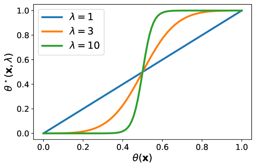
$q({\bm{\theta}}|{\bm{X}},\lambda)$

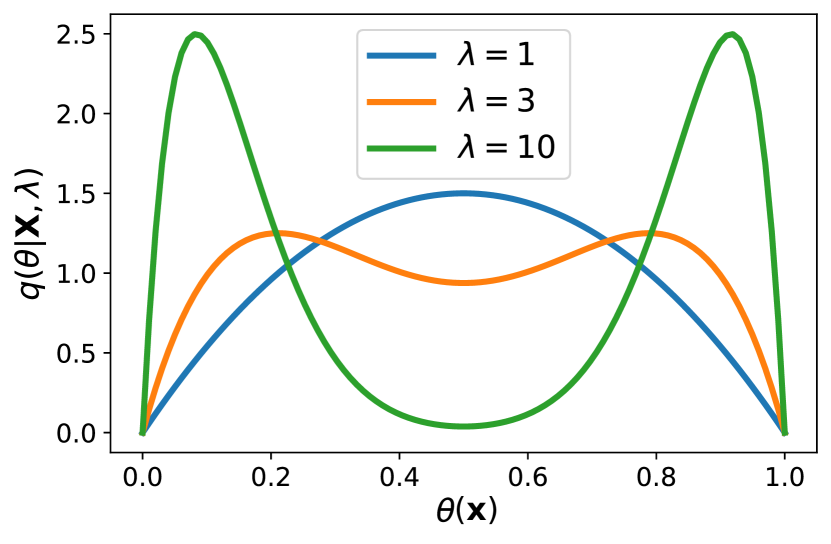
$q({\bm{\theta}}|{\bm{X}},\lambda)$

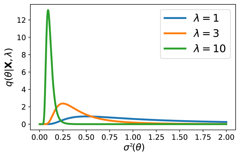
Figure 2.1: Illustration of the new likelihood $q({\bm{y}}|{\bm{x}},{\bm{\theta}},\lambda)$ and priors $q({\bm{\theta}}|{\bm{X}},\lambda)$. In the left and middle figures, the original likelihood is in the form of the Bernoulli distribution. The left figure demonstrates the transformation from $\theta({\bm{x}})$ to $\theta^{\star}({\bm{x}},\lambda):=\frac{\theta({\bm{x}})^{\lambda}}{\theta({\bm{x}})^{\lambda}+(1-\theta({\bm{x}}))^{\lambda}}$. In the middle figure, we display a Beta-Binomial example, where the prior, initialized as a Beta distribution, is updated with a single Bernoulli-distributed sample. In the right figure, we display the new prior, initialized as an inverse-gamma prior and updated with a Gaussian likelihood with a single observation.

Regression example

Consider the case where the original likelihood is Gaussian, defined as $p({\bm{y}}|{\bm{x}},{\bm{\theta}})=\mathcal{N}(\mu(\bm{x},{\bm{\theta}}),\sigma^{2}({\bm{\theta}}))$, where the variance is input-independent, as typically seen in many regression problems. Then, following Equation 2.8, the new likelihood corresponds to a scaling in the variance, given by $q({\bm{y}}|{\bm{x}},{\bm{\theta}},\lambda)=\mathcal{N}(\mu(\bm{x},{\bm{\theta}}),\tfrac{\sigma^{2}({\bm{\theta}})}{\lambda^{2}})$. Thus, as $\lambda$ increases, the tempered likelihood $q({\bm{y}}|{\bm{x}},{\bm{\theta}},\lambda)$ induces a proper Gaussian likelihood with reduced variance, i.e., a new likelihood with lower aleatoric uncertainty.

Classification example

Consider the case of a binary classification problem where the original conditional likelihood is Bernoulli, defined as $p({\bm{y}}|{\bm{x}},{\bm{\theta}})=\theta({\bm{x}})^{y}(1-\theta({\bm{x}}))^{1-y}$ with $y\in\{0,1\}$ and the input-dependent parameter function $\theta({\bm{x}})\in[0,1]$, which is usually implemented by a neural network with a softmax activation function in the last layer. Then, following Equation 2.8, the new conditional likelihood $q({\bm{y}}|{\bm{x}},{\bm{\theta}},\lambda)=\theta^{*}({\bm{x}},\lambda)^{y}(1-\theta^{*}({\bm{x}},\lambda))^{1-y}$ also follows a Bernoulli distribution with a different parameter function $\theta^{*}({\bm{x}},\lambda)=\frac{\theta({\bm{x}})^{\lambda}}{\theta({\bm{x}})^{\lambda}+(1-\theta({\bm{x}}))^{\lambda}}\in[0,1]$. The function $\theta^{*}({\bm{x}},\lambda)$ is displayed in Figure 2.1 (left). When $\lambda$ increases, the parameter function that defines the new Bernoulli likelihood becomes more extreme, resulting in a new likelihood with lower aleatoric uncertainty.

In both cases, we see that as suggested by Proposition 2.5, as $\lambda$ increases, the new conditional likelihoods $q({\bm{y}}|{\bm{x}},{\bm{\theta}},\lambda)$ have lower entropy, i.e., lower aleatoric uncertainty. In Sections 2.5.2 and 2.5.3, we will further explore the implications of this finding and its connection to existing literature.

2.4.2 How $\lambda$ influences the new priors

On the other hand, according to Proposition 2.4, using the tempered posteriors implies implicitly using the prior $q({\bm{\theta}}|{\bm{X}},\lambda)$. Such prior depends on the unlabelled training data ${\bm{X}}$. On top of that, the functional form of the likelihood function is defined by the probabilistic model family through the term $\int p({\bm{y}}|{\bm{x}},{\bm{\theta}})^{\lambda}d{\bm{y}}$ for ${\bm{x}}\in{\bm{X}}$. Hence, models ${\bm{\theta}}$ that yield a large value for this term across most of the training data ${\bm{x}}\in{\bm{X}}$ will be assigned larger probability mass by the new prior. We will showcase this effect in both regression and binary classification problems. Moreover, we will see how the new prior $q({\bm{\theta}}|{\bm{X}},\lambda)$ with $\lambda>1$ favors those models within the model class that yield likelihoods with lower aleatoric uncertainty on the training data ${\bm{X}}$.

Regression example

Consider the case where the original likelihood is Gaussian, defined as $p({\bm{y}}|{\bm{x}},{\bm{\theta}})=\mathcal{N}(\mu(\bm{x},{\bm{\theta}}),\sigma^{2}({\bm{\theta}}))$, where the variance is input-independent, as typically seen in many regression problems. A common parametrization involves ${\bm{\theta}}=({\bm{w}},\gamma)$, where ${\bm{w}}$ refer to the weights of the neural network defining the function $\mu(\bm{x},{\bm{\theta}})$ and $\gamma>0$ is a parameter encoding the variance of the Gaussian likelihood such that $\sigma^{2}({\bm{\theta}})=\gamma$. The prior $p({\bm{\theta}})$ is then defined as $p({\bm{\theta}})=p({\bm{w}})p(\gamma)$, where $p({\bm{w}})$ is usually a Gaussian distribution with a diagonal covariance matrix, and $p(\gamma)$ is usually defined in terms of an inverse-gamma distribution. Following Equation 2.8, the new prior would be expressed as $q({\bm{\theta}}|{\bm{X}},\lambda)=q({\bm{w}}|{\bm{X}},\lambda)q(\gamma|{\bm{X}},\lambda)$, where each term

$$q({\bm{w}}|{\bm{X}},\lambda)=p({\bm{w}})\quad,\quad q(\gamma|{\bm{X}},\lambda)\propto p(\gamma)/\gamma^{n(\lambda-1)}\,.$$

Figure 2.1 (right) plots the density of $q(\gamma|{\bm{X}},\lambda)$ when only one data is observed, with various $\lambda>1$ values when $p(\gamma)$ is an inverse-gamma prior. For larger $\lambda$ values, this new prior will assign more probability mass to models defining a likelihood with smaller variance or, equivalently, smaller aleatoric uncertainty.

Classification example

Consider another case where the original conditional likelihood is Bernoulli, defined as $p({\bm{y}}|{\bm{x}},{\bm{\theta}})=\theta({\bm{x}})^{y}(1-\theta({\bm{x}}))^{1-y}$ with $y\in\{0,1\}$ and $\theta({\bm{x}})\in[0,1]$, as commonly used in binary classification problems. Also, take any prior $p({\bm{\theta}})$. Then, following Equation 2.8, the new prior is expressed as

$$q({\bm{\theta}}|{\bm{X}},\lambda)\propto p({\bm{\theta}})\prod_{{\bm{x}}\in{\bm{X}}}\Big{(}\theta({\bm{x}})^{\lambda}+(1-\theta({\bm{x}}))^{\lambda}\Big{)}\,.$$

Figure 2.1 (middle) illustrates the transformation of the prior for a Beta-Binomial model with a single training sample. Initially, the prior $p({\bm{\theta}})$ is taken as a Beta distribution, while the likelihood of this single data is Bernoulli. As $\lambda\geq 1$ increases, the new prior assigns more probability mass to models where $\theta({\bm{x}})$ is close to either $1$ or $0$. In other words, this new prior assigns more probability mass to models that assign more extreme probabilities to the training data (i.e., models with lower aleatoric uncertainty). Note that the prior does not consider how accurately these models classify the training data, but only the extremity of the probabilities assigned to the training data.

We will discuss in Section 2.5.4 further implications of this finding and how it relates to the literature.

2.4.3 Generalized ELBOs are also proper ELBOs

Generalized ELBOs, characterized by scaling the KL divergence term using a hyper-parameter $\lambda$, have found widespread application in many studies (WRVS+20). This popularity stems from the demonstrated ability to adjust $\lambda$ to improve the predictive accuracy of variational approximations:

$$q^{\star}_{\lambda}:=\operatorname*{arg\,min}_{r\in\Pi}\mathbb{E}_{r}[-\ln p(D|{\bm{\theta}})]+\frac{1}{\lambda}\operatorname{KL}(r({\bm{\theta}}),p({\bm{\theta}}))\,,$$ (2.10)

where $\Pi$ defines the variational family. Critics have pointed out a flaw in the above generalized ELBO when $\lambda$ deviates from $1$, as it no longer functions as a true lower bound for the marginal likelihood. However, Proposition 2.4 can be used to justify that such a variational posterior $q^{\star}_{\lambda}$ still emerges from minimizing a valid ELBO. Specifically, it is constructed based on the revised likelihood and prior functions as follows:

$$q^{\star}_{\lambda}=\operatorname*{arg\,min}_{r\in\Pi}\mathbb{E}_{r}[-\ln q({\bm{Y}}|{\bm{X}},{\bm{\theta}},\lambda)]+\operatorname{KL}(r({\bm{\theta}}),q({\bm{\theta}}|{\bm{X}},\lambda))\,.$$ (2.11)

Consequently, this analysis shows that using generalized ELBOs as Equation 2.10 perfectly adheres to variational and Bayesian principles.

2.4.4 Insights and implications from the section

In this section, we show that employing tempered posteriors seamlessly fits within a Bayesian framework, which streamlines and enriches the use of diverse likelihood and prior functions.

With the characterization in Section 2.3, observing CPE implies that the tempered posterior, which implicitly employs the new likelihood and priors defined in Equation 2.8 is better specified in comparison to the original Bayesian posterior. The alignment with the underlying data-generating distribution is easily achieved by tempering. Consequently, tempered posteriors offer a simple, computationally efficient, and theoretically sound approach to mitigate the underfitting problem often encountered in contemporary Bayesian deep learning methods.

Furthermore, as discussed in Section 2.4.1 and Section 2.4.2, increasing $\lambda$ results in likelihoods with lower aleatoric uncertainty and priors that favor models yielding such likelihoods on the training data $X$. Therefore, the occurrence of CPE in contemporary Bayesian deep learning indicates that the models currently employed in the field often underfit the data by assuming models with too high aleatoric uncertainty. This strengthens our understanding of the CPE as a consequence of underfitting, resulting from poorly specified likelihood and prior functions.

We will further expand on and discuss how these implications relate to the literature in Section 2.5.

2.5 Likelihood misspecification, prior misspecification and the CPE

2.5.1 CPE, approximate inference, and NNs

As mentioned in the introduction, several works have discussed that CPE is an artifact of inappropriate approximate inference methods, especially in the context of the highly complex posterior that emerge from neural networks (WRVS+20). There are occasions suggesting that if the approximate inference method is accurate enough, the CPE disappears (IVHW21). However, Proposition 2.1 shows that when $\lambda$ is made larger than 1, the training loss of the exact Bayesian posterior decreases; if the test loss decreases too, the exact Bayesian posterior underfits. It means that even if the inference method is accurate, we can still observe the CPE due to underfitting. In fact, Figures 2.2 and 2.3 shows examples of a Bayesian linear regression model learned on synthetic data. Here, the exact Bayesian posterior can be computed, and it is clear from Figures 2.3(b) and 2.2(c) that the CPE can occur in Bayesian linear regression with exact inference. Although simple, the setting is articulated specifically to mimic the classification tasks using BNNs where CPE was observed. In particular, the linear model has more parameters than observations (i.e., it’s overparameterized). We also note that adlam2020cold presents similar findings and observations for Gaussian process regression.

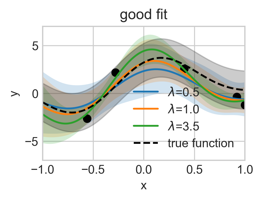
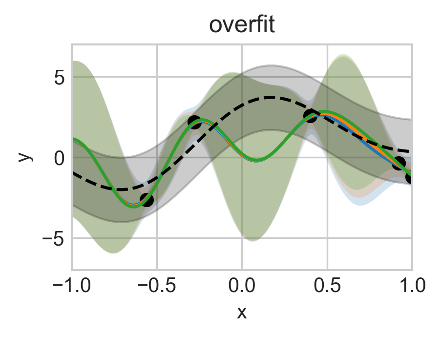
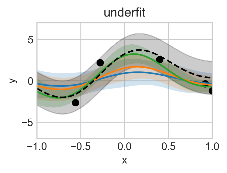
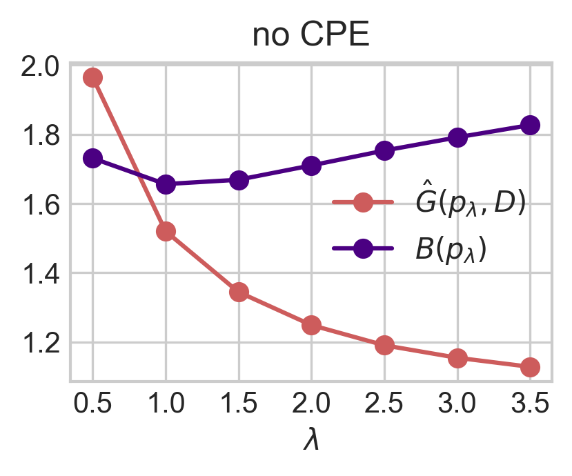
(a) No likelihood or prior misspecification

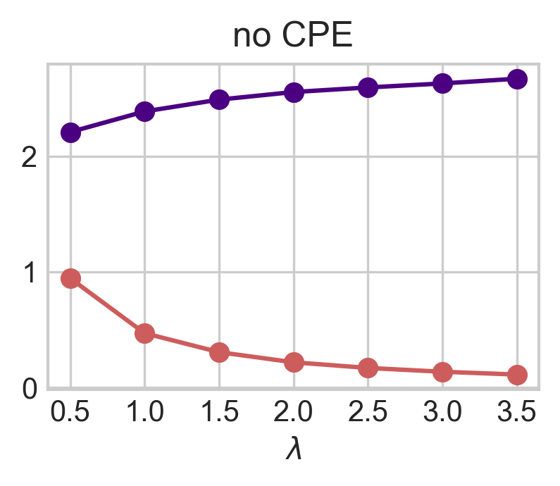
(b) Likelihood misspecification case I

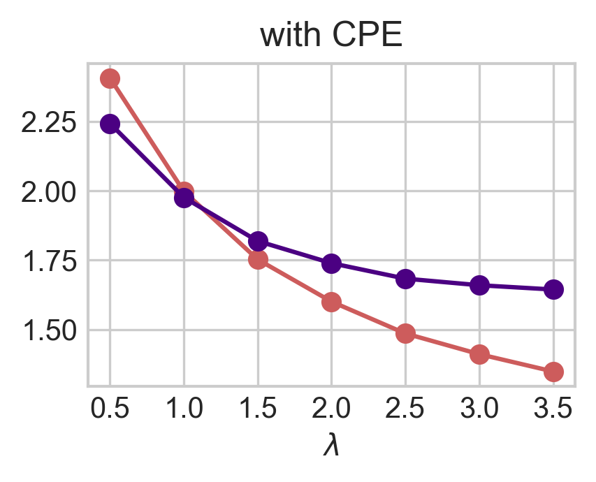
(c) Only with prior misspecification

Figure 2.2: 1. The CPE occurs in Bayesian linear regression with exact inference. 2. Model misspecification can lead to overfitting and to a “warm” posterior effect (WPE). Every column displays a specific setting, as indicated in the caption. The first row shows exact Bayesian posterior predictive fits for three different values of the tempering parameter $\lambda$. The second row shows the Gibbs loss $\hat{G}(p_{\lambda},D)$ (aka training loss) and the Bayes loss $B(p_{\lambda})$ (aka testing loss) with respect to $\lambda$. The experimental details are given in Appendix 2.8.4.

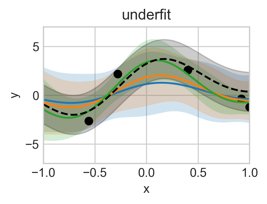
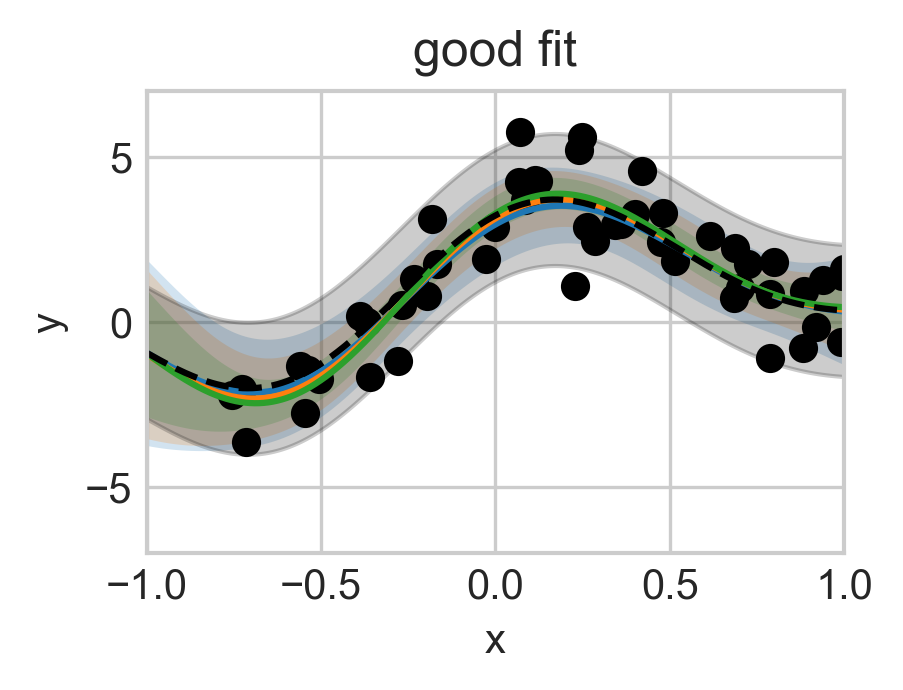
(a) No likelihood or prior misspecification

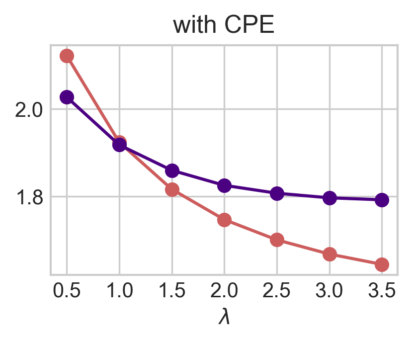
(b) Likelihood misspecification case II

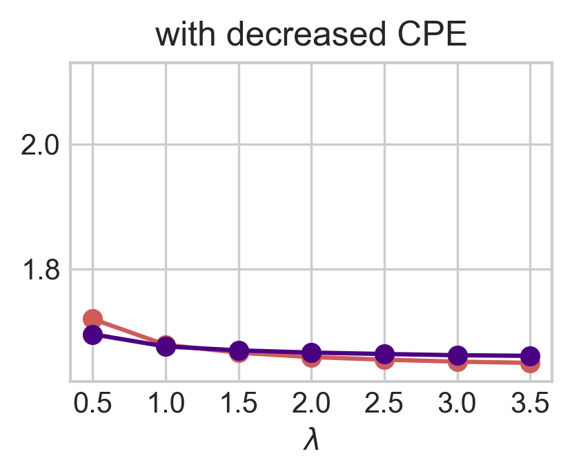
(c) Same as (b) but with 50 data points

Figure 2.3: Extended results of Figure 2.2 with more configurations of model misspecification.

2.5.2 Model misspecification, CPE, and underfitting

Prior and/or likelihood misspecification can lead Bayesian methods to both underfitting and overfitting, as widely discussed in the literature (domingos2000bayesian; immer2021improving; KMIW22). We illustrate this using a Bayesian linear regression model: Figures 2.3(b) and 2.2(c) show how the Bayesian posterior underfits due to likelihood and prior misspecification, respectively. On the other hand, Figure 2.2(b) showcases a scenario where likelihood misspecification can perfectly lead to overfitting as well, giving rise to what we term a “warm” posterior effect (WPE), i.e., there exist other posteriors ($p_{\lambda}$ with $\lambda<1$) with lower testing loss, which, at the same time, have higher training loss due to Proposition 2.1. As a result, to describe CPE merely as a model misspecification issue without acknowledging underfitting offers a narrow interpretation of the problem.

The examples presented in Figures 2.2 and 2.3 help illustrate the results of Proposition 2.4 and provide concrete demonstrations of the theoretical insights discussed: when CPE shows up, tuning $\lambda$ is akin to finding another Bayesian posterior with a less misspecified likelihood and prior.However, we note that in this particular Bayesian linear regression setup, the new prior $q({\bm{\theta}}|{\bm{X}},\lambda)$ is always equal to initial prior $p({\bm{\theta}})$ because the variance of the likelihood is assumed to be constant. Therefore, the analysis of the regression case in Section 2.4.2 does not directly apply here.

In the discussion regarding likelihood, we refer to the regression example in Section 2.4.1. Let’s first have a look at Figure 2.3(b), where the Gaussian likelihood model has a larger variance than the true data-generating process. By increasing $\lambda$, we obtain a likelihood model with a smaller variance (divided by $\lambda^{2}$, as shown in the regression example in Section 2.4.1), i.e., we induce a new likelihood with lower aleatoric uncertainty (Proposition 2.5). Such a new model is closer to the true data-generating distribution and less misspecified, thus enjoying better performance. The opposite can be seen in Figure 2.2(b), where the Gaussian likelihood model has a lower variance than the true data-generating distribution and the WPE occurs.

2.5.3 The likelihood misspecification argument

Likelihood misspecification has also been identified as a cause of CPE, especially in cases where the dataset has been curated (Ait21; KMIW22). Data curation often involves carefully selecting samples and labels to improve the quality of the dataset. As a result, the curated data-generating distribution typically presents very low aleatoric uncertainty, meaning that $\nu({\bm{y}}|{\bm{x}})$ usually takes values very close to either $1$ or $0$. However, as previously discussed in (Ait21; KMIW22), the standard likelihoods used in deep learning for image classification, like softmax or sigmoid, tend to allocate more spread-out probabilities to the outcomes, implicitly reflecting a higher level of aleatoric uncertainty. Therefore, their use in curated datasets that exhibit low uncertainty made them misspecified (KMIW22; FGAO+22). To address this issue, alternative likelihood functions like the Noisy-Dirichlet model (KMIW22, Section 4) have been proposed, which better align with the characteristics of the curated data. On the other hand, introducing noise labels also alleviates the CPE, as demonstrated in Ait21. By introducing noise labels, we intentionally increase aleatoric uncertainty in the data-generating distribution, which aligns better with the high aleatoric uncertainty assumed by the standard Bayesian deep networks (KMIW22). Consequently, according to these works, the CPE can be strongly alleviated when the likelihood misspecification is addressed.

Our theoretical analysis aligns with these findings in Sections 2.4.1 and 2.4.4: fitting low aleatoric uncertainty data-generating distributions, e.g., $\nu(y|{\bm{x}})\in\{0.01,0.99\}$, with high aleatoric uncertainty likelihood functions e.g., $p(y|{\bm{x}},{\bm{\theta}})\in[0.2,0.8]$, induces underfitting, and thus, CPE. The presence of underfitting is not mentioned at all by any of these previous works (Ait21; KMIW22). On top of that, using Propositions 2.4 and 2.5, our work explains why the likelihood implicitly used by the tempered posterior with $\lambda>1$ provides better generalizaton performance. Because, in this case, we are using a likelihood $q({\bm{\theta}}|{\bm{X}},\lambda)$ (Equation 2.8) with lower aleatoric uncertainty, which better aligns with the low aleatoric uncertainty data-generating distribution induced by curated datasets, thus reducing the degree of model misspecification.

Figures 2.4(a) and 2.4(b), along with Figures 2.5(a) and 2.5(b), illustrate this point through a regular multi-class classification task on a curated benchmark dataset. Both scenarios utilize the same narrow prior. The distinction in Figure 2.4(b) lies in the adoption of a tempered softmax likelihood, defined as $p(y|x,\theta)=\left(1+\exp\left(-\gamma\,\text{{logits}}(x,\theta)\right)\right)^{-1}$, with $\gamma=2$, compared to $\gamma=1$ in Figure 2.4(a). This tempered softmax likelihood, more closely aligned with the dataset’s low aleatoric uncertainty as outlined by (DBLP:conf/icml/GuoPSW17), leads to a reduced incidence of CPE in Figure 2.4(b) compared to Figure 2.4(a). From the perspective of Proposition 2.4 and specifically Proposition 2.5, the intrinsic lower aleatoric uncertainty of the likelihood used in Figure 2.4(b) (softmax with $\gamma=2$) makes the potential for improvement through increasing $\lambda$ somewhat limited, resulting in a less pronounced CPE compared to Figure 2.4(a). It is, however, important to highlight the critical interaction between the likelihood and the prior, as we dicuss next.

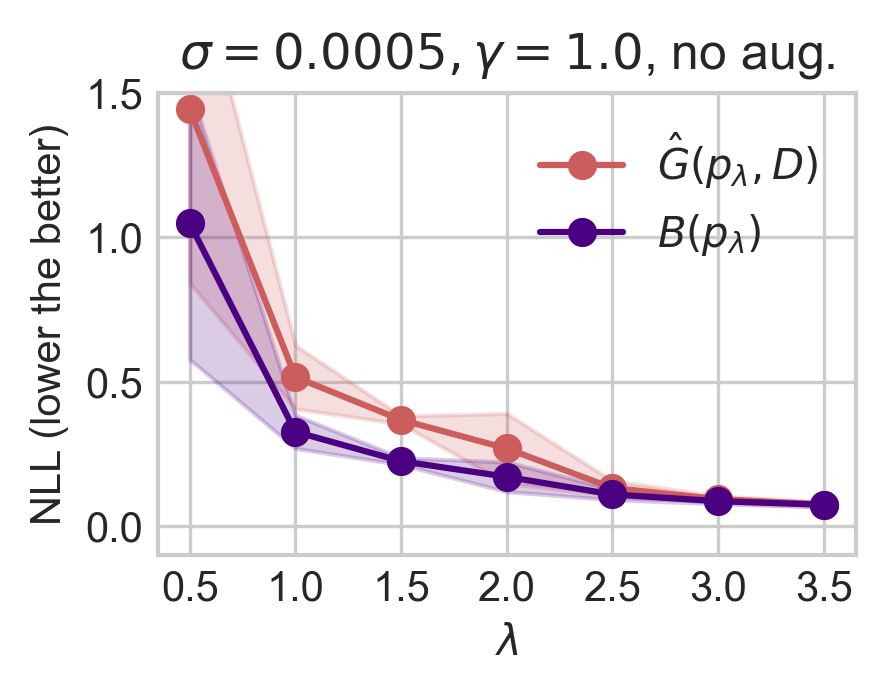
(a) Narrow prior and standard softmax

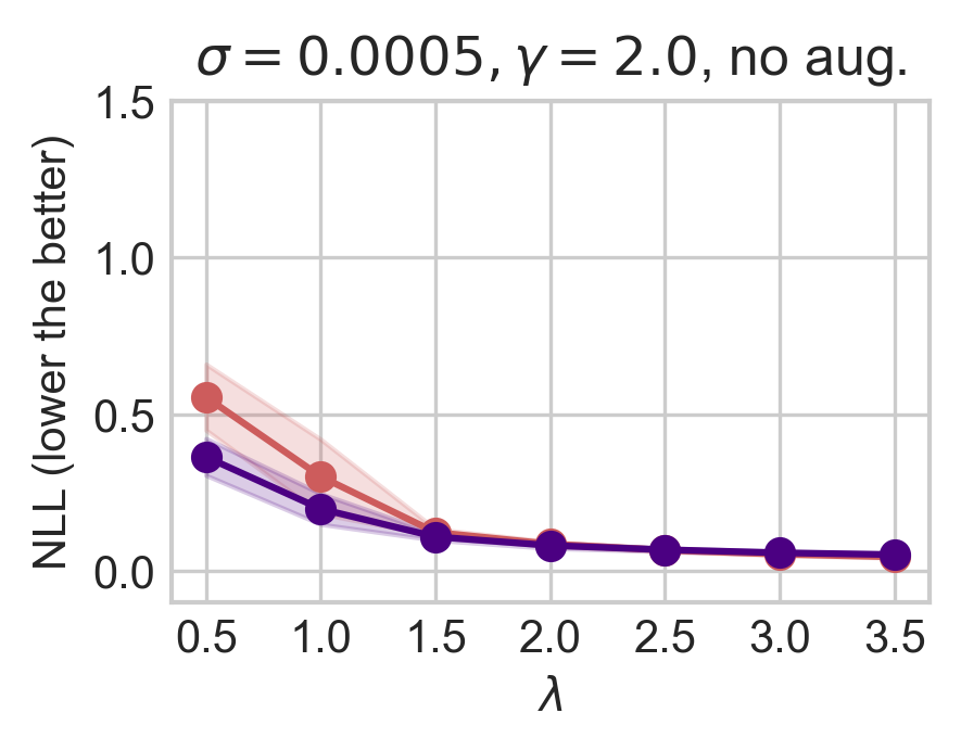
(b) Narrow prior and tempered softmax

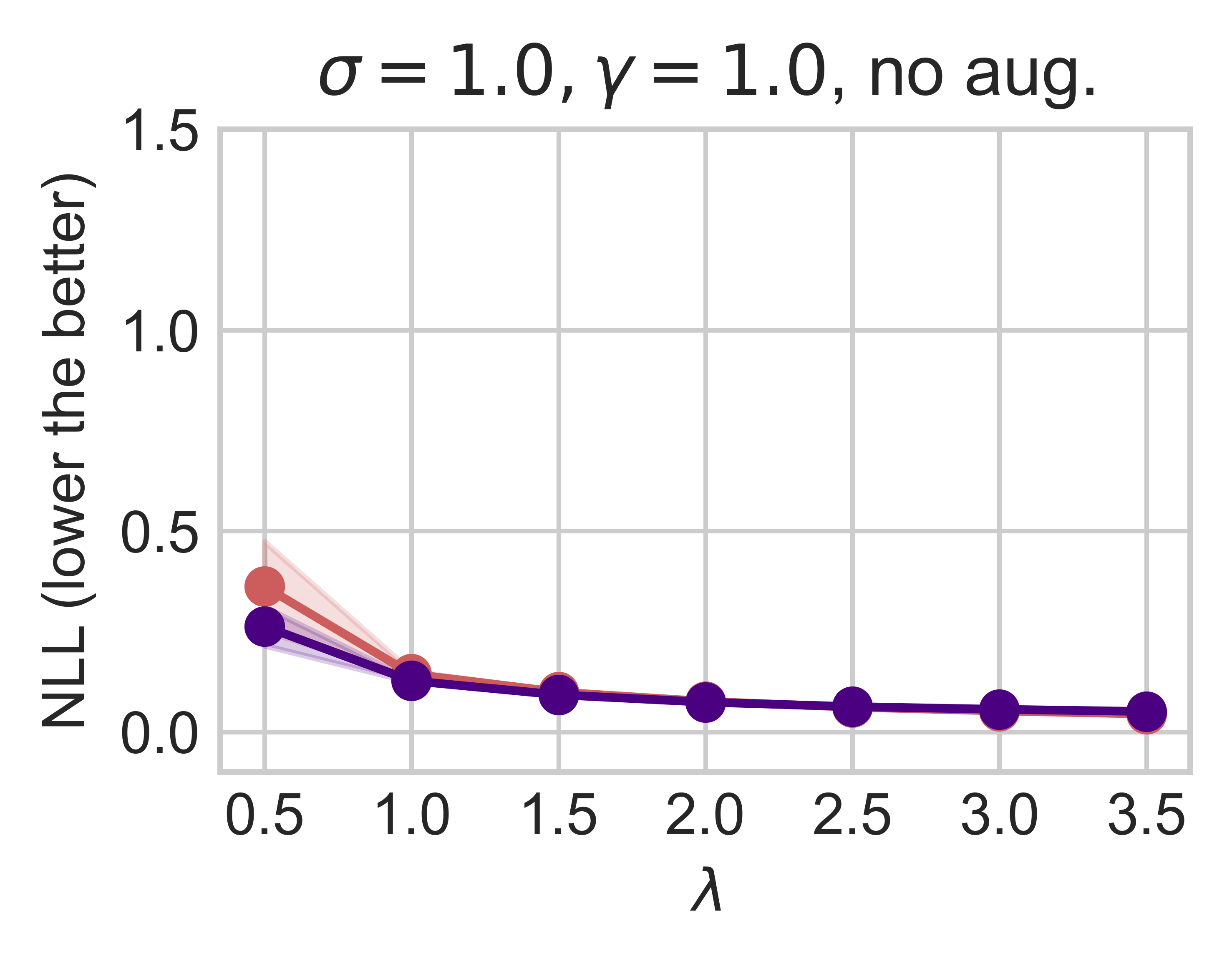
(c) Standard prior and standard softmax

Figure 2.4: Experimental illustrations for the arguments in Section 2.5 using small CNN via SGLD on MNIST. We show similar results on Fashion-MNIST with small CNN and CIFAR-10(0) with ResNet-18 in Appendix LABEL:app:sec:experiment-approx. Figures 2.4(a) to 2.4(c) illustrate the arguments in Section 2.5. Figure 2.4(c) uses the standard prior ($\sigma=1$) and the standard softmax ($\gamma=1$) for the likelihood without applying DA. Figure 2.4(a) follows a similar setup except for using a narrow prior. Figure 2.4(b) uses a narrow prior as in Figure 2.4(a) but with a tempered softmax that results in a lower aleatoric uncertainty. We report the training loss $\hat{G}(p_{\lambda},D)$ and the testing losses, $B(p_{\lambda})$ and $G(p_{\lambda})$, from 10 samples of the small Convolutional neural network (CNN) via Stochastic Gradient Langevin Dynamics (SGLD). We show the mean and standard error across three different seeds. For additional experimental details, please refer to Appendix LABEL:app:sec:experiment-approx.

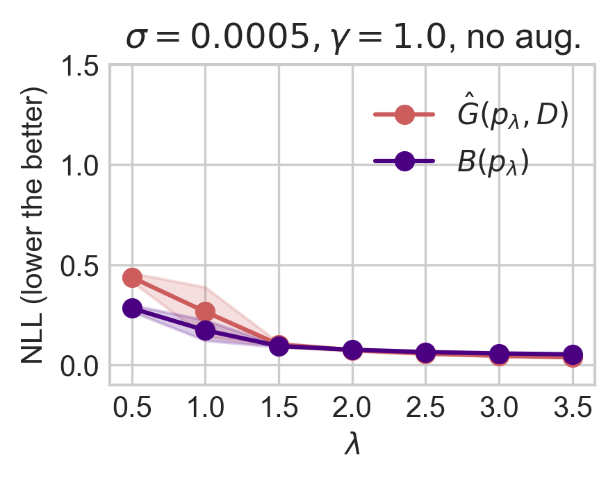
(a) Narrow prior and standard softmax

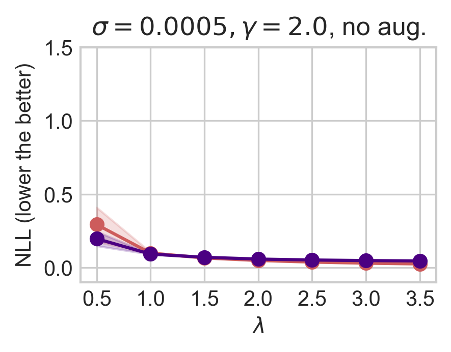
(b) Narrow prior and tempered softmax

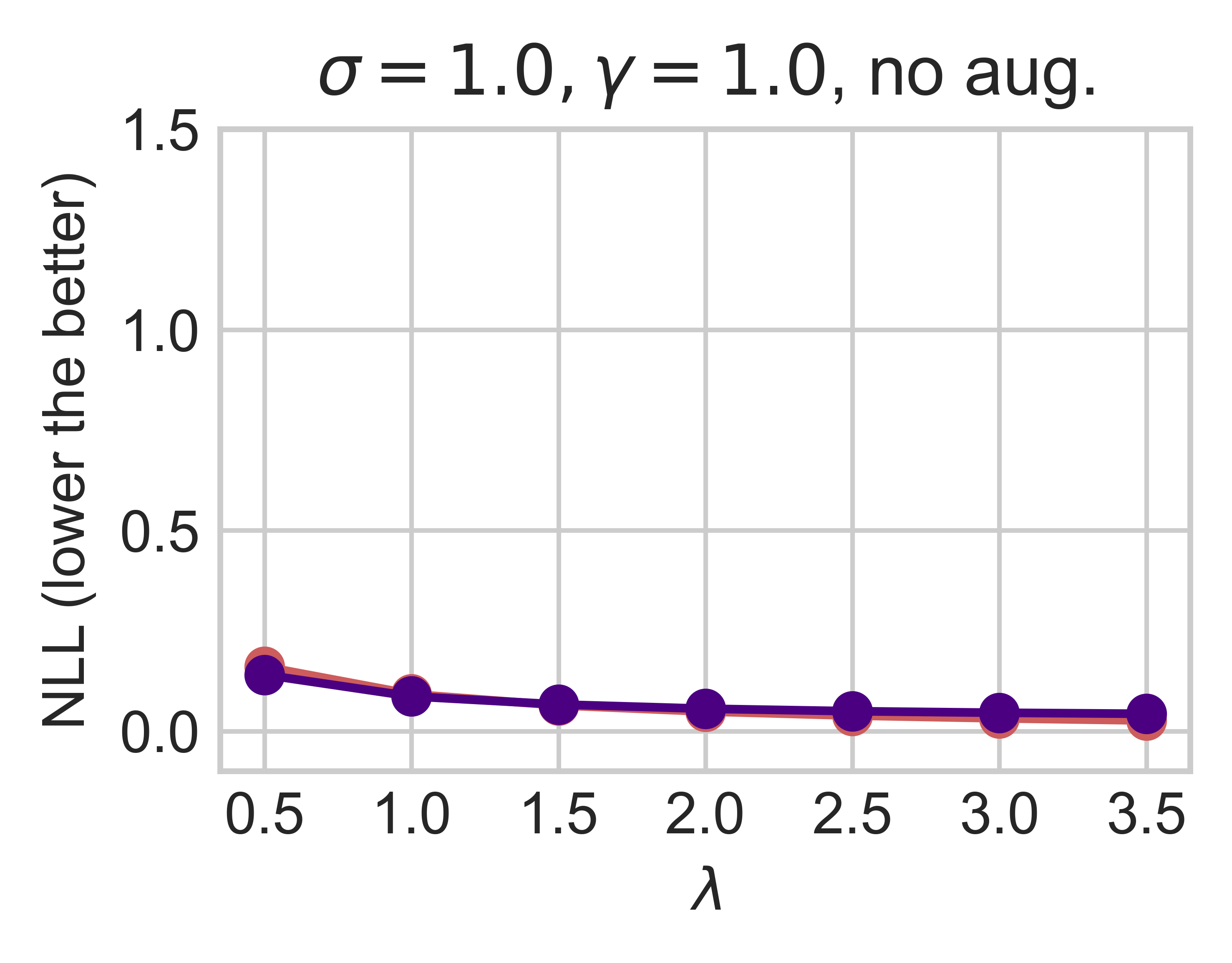
(c) Standard prior and standard softmax

Figure 2.5: Experimental illustrations for the arguments in Section 2.5 using large CNN via SGLD on MNIST. We show similar results on Fashion-MNIST with large CNN and CIFAR-10(0) with ResNet-50 in Appendix LABEL:app:sec:experiment-approx. The experiment setup is similar to the setups in Figure 2.4 but with a large CNN. Please refer to Appendix LABEL:app:sec:experiment-approx for further details on the model.

2.5.4 The prior misspecification argument

As highlighted in previous works, such as in WRVS+20; FGAO+22, isotropic Gaussian priors are commonly chosen in modern Bayesian neural networks for the sake of tractability in approximate Bayesian inference rather than chosen based on their alignment with our actual beliefs. Given that the presence of the CPE implies that either the likelihood and/or the prior are misspecified, and given that neural networks define highly flexible likelihood functions, there are strong reasons for thinking these commonly used priors are misspecified. Notably, the experiments conducted by FGAO+22 demonstrate that the CPE can be mitigated in fully connected neural networks when using heavy-tailed prior distributions that better capture the weight characteristics typically observed in such networks. However, such priors were found to be ineffective in addressing the CPE in convolutional neural networks (FGAO+22), indicating the challenges involved in designing effective Bayesian priors within this context.

Our theoretical analysis provides a deeper insight into these observations. As discussed in Section 2.3, the absence of underfitting means the absence of CPE. This suggests flexible likelihood functions may still result in posteriors that underfit, due to the prior’s tendency to overly regularize. This may incur CPE when the strong prior fails to allocate enough probability to models that both fit the training data well and exhibit good generalization capabilities. As detailed in Section 2.4.2, employing tempered posteriors with $\lambda>1$ effectively defines a conditional prior $q({\bm{\theta}}|{\bm{X}},\lambda)$ that favors models with lower aleatoric uncertainty. If such models align better with the training data compared to the original prior, then we may observe CPE. Also, the conditional prior $q({\bm{\theta}}|{\bm{X}},\lambda)$ with $\lambda>1$ can be considered better specified than the original prior $p({\bm{\theta}})$.

Figures 2.4(a) and 2.4(c) exemplify this situation. The prior in the case of Figures 2.4(a) is very narrow ($\sigma=0.0005$), inducing strong regularization. Such a narrow prior results in a posterior that severely underfits the training data, evident from the high empirical Gibbs loss that deviates significantly from zero. Additionally, we observe a strong CPE. On the other hand, with a flatter prior in the case of Figure 2.4(c), the CPE is considerably diminished. According to the discussion above and Sections 2.4.2 and 2.4.4, we know that the flatter prior allocates more probability mass to preferred models. Also, such preferred models have lower aleatoric uncertainty than the ones assigned initially by the narrow prior in the former case. To elaborate further, in the former case, the new prior $q({\bm{\theta}}|{\bm{X}},\lambda)$ with $\lambda>1$ would place much more probability mass to models with lower aleatoric uncertainty than the narrow prior and strongly alleviating underfitting. In the second case, since the flatter prior already distributes probability mass more broadly across the model class, the room to shift probability mass to models with lower aleatoric uncertainty is more limited than that from a narrower prior, resulting in a milder CPE.

2.5.5 Model size, sample size in relation to CPE and underfitting

Larger models have the capacity to fit data more effectively, while smaller models are more likely to underfit. As we have argued that if there is no underfitting, there is no CPE, we expect that the size of the model has an impact on the strength of CPE as well. We demonstrate in Figure 2.4 and Figure 2.5. Specifically, in our experiments presented in Figure 2.4, we use a relatively small convolutional neural network (CNN), which has a more pronounced underfitting behavior, and this indeed corresponds to a stronger CPE. On the other hand, we employ a larger CNN in Figure 2.5, which has less underfitting, and we see the CPE is strongly alleviated. Actually, this effect can be directly inferred from Theorem 2.3. For an extremely flexible model capable of perfectly fitting both the original training samples and new samples, this theorem suggests that a CPE should not be expected, as the model’s fit on the original data remains perfect, even when new examples are introduced.

Theorem 2.3 can also be used to understand why small models in the presence of large training data sets do not exhibit CPE. We empirically illustrate this point in Figures 2.2 and 2.3. In particular, Figure 2.3(b) and Figure 2.3(c) use the same (small) regression models and settings where the only difference is that Figure 2.3(b) uses 5 data points while Figure 2.3(c) uses 50 data points. In situations where a model possesses limited flexibility and the training set is large, including additional examples should barely affect the fit of the original training data because the Bayesian posterior is highly concentrated and will be barely affected by a single extra sample. Then, as predicted by Theorem 2.3, CPE in Figure 2.3(c) is much less significant than in Figure 2.3(b).

Finally, it’s worth noting that Figure 11 in WRVS+20 shows the opposite effect, where larger models exhibit much stronger CPE compared to shallower or narrower versions of the same architectures. However, it’s important to recognize that WRVS+20 studied full-tempering, whereas our work focuses on likelihood-tempering. For full-tempering, Proposition 2.1 does not necessarily hold. Intuitively, since $\lambda$ operates on both the likelihood (data) and the prior (regularization) simultaneously, the effect of increasing $\lambda$ is mixed, not necessarily improving the fit on the training data. Consequently, the CPE brought by full-tempering as $\lambda$ increases does not necessarily coincide with better training loss, as the training loss may not be improvable. As a result, the CPE observed with full-tempering cannot be interpreted solely as underfitting. Therefore, for full-tempering, increasing model capacity may not achieve a lower degree of CPE, unlike the behavior we observed in our case focusing on likelihood-tempering.

2.6 Data augmentation (DA) and the CPE

Machine learning is applied to many different fields and problems. In many of them, the data-generating distribution is known to have properties that can be exploited to generate new data samples (shorten2019survey) artificially. This is commonly known as data augmentation (DA) and relies on the property that for a given set of transformations $H=\{h:\cal X\rightarrow\cal X\}$, the data-generating distribution satisfies $\nu({\bm{y}}|{\bm{x}})=\nu({\bm{y}}|h({\bm{x}}))$ for all $h\in H$. In practice, not all the transformations are applied to every single data. Instead, a probability distribution (usually uniform) $\mu_{H}$ is defined over $H$, and augmented samples are drawn accordingly. As argued in NGGA+22, the use of data augmentation when training Bayesian neural networks implicitly targets the following (pseudo) log-likelihood, denoted $\hat{L}_{\text{\tiny{DA}}}(D,{\bm{\theta}})$ and defined as

$$\hat{L}_{\text{\tiny{DA}}}(D,{\bm{\theta}})=\frac{1}{n}\sum_{i\in[n]}\mathbb{E}_{h\sim\mu_{H}}\left[-\ln p({\bm{y}}_{i}|h({\bm{x}}_{i}),{\bm{\theta}})\right]\,,$$ (2.12)

where data augmentation provides unbiased estimates of the expectation under the set of transformations using Monte Carlo samples (i.e., random data augmentations).

Although some argue that this data-augmented (pseudo) log-likelihood “does not have a clean interpretation as a valid likelihood function” (WRVS+20; IVHW21), we do not need to enter into this discussion to understand why the CPE emerges when using the generalized Bayes posterior (bissiri2016general_6) associated to this (pseudo) log-likelihood, which is the main goal of this section. We call this posterior the DA-tempered posterior and is denoted by $p_{\lambda}^{\text{\tiny{DA}}}({\bm{\theta}}|D)$. The DA-tempered posterior can be expressed as the global minimizer of the following learning objective,

$$p_{\lambda}^{\text{\tiny{DA}}}({\bm{\theta}}|D)=\operatorname*{arg\,min}_{\rho}\mathbb{E}_{\rho}[n\hat{L}_{\text{\tiny{DA}}}(D,{\bm{\theta}})]+\frac{1}{\lambda}\operatorname{KL}(\rho({\bm{\theta}}|D),p({\bm{\theta}}))\,.$$ (2.13)

This is similar to Equation 2.3 but now using $\hat{L}_{\text{\tiny{DA}}}(D,{\bm{\theta}})$ instead of $\hat{L}(D,{\bm{\theta}})$, where we recall the notation $\hat{L}(D,{\bm{\theta}})=-\tfrac{1}{n}\ln p(D|{\bm{\theta}})$. Hence, the resulting DA-tempered posterior is given by $p^{\text{\tiny{DA}}}_{\lambda}({\bm{\theta}}|D)\propto e^{-n\lambda\hat{L}_{\text{\tiny{DA}}}(D,{\bm{\theta}})}p({\bm{\theta}})$. In comparison, the tempered posterior $p_{\lambda}({\bm{\theta}}|D)$ in Equation 2.2 can be similarly expressed as $e^{-n\lambda\hat{L}(D,{\bm{\theta}})}p({\bm{\theta}})$.

There is large empirical evidence that DA induces a stronger CPE (WRVS+20; IVHW21; FGAO+22). Indeed, many of these studies show that if CPE is not present in our Bayesian learning settings, using DA makes it appear. According to our previous analysis, this means that the use of DA induces a stronger underfitting. To understand why this is case, we will take a step back and begin analyzing the impact of DA in the so-called Gibbs loss of the DA-Bayesian posterior $p_{\lambda=1}^{\text{\tiny{DA}}}$ rather than the Bayes loss, as this will help us in understanding this puzzling phenomenon.

2.6.1 Data augmentation and CPE on the Gibbs loss

The expected Gibbs loss of a given posterior $\rho$, denoted $G(\rho)$, is a commonly used metric in the theoretical analysis of the generalization performance of Bayesian methods (germain2016pac; masegosa2020learning). The Gibbs loss represents the average of the expected log-loss of individual models under the posterior $\rho$, that is,

$$G(\rho)=\mathbb{E}_{\rho}[L({\bm{\theta}})]=\mathbb{E}_{\rho}[\mathbb{E}_{\nu}[-\ln[p({\bm{y}}|{\bm{x}},{\bm{\theta}})]]\,.$$

In fact, Jensen’s inequality confirms that the expected Gibbs loss serves as an upper bound for the Bayes loss, i.e., $G(\rho)\geq B(\rho)$. This property supports the expected Gibbs loss to act as a proxy of the Bayes loss, which justifies its usage in gaining insights into how DA impacts the CPE.

We will now study whether data augmentation can cause a CPE on the Gibb loss. In other words, we will examine whether increasing the parameter $\lambda$ of the DA-tempered posterior leads to a reduction in the Gibbs loss. This can be formalized by extending Definition 2.1 to the expected Gibbs loss by considering its derivative $\frac{d}{d\lambda}G(p_{\lambda})$ at $\lambda=1$, which can be represented as follows:

$$\frac{d}{d\lambda}G(p_{\lambda})_{|\lambda=1}=-\mathrm{COV}_{p_{\lambda=1}}\big{(}n\hat{L}(D,{\bm{\theta}}),L({\bm{\theta}})\big{)}\,.$$ (2.14)

Where $\mathrm{COV}(X,Y)$ denotes the covariance of $X$ and $Y$. Again, due to the page limit, we postpone the necessary proofs in this section to Appendix 2.8.3.

With this extended definition, if Equation 2.14 is negative, we can infer the presence of CPE for the Gibbs loss as well. Based on this, we say that DA induces a stronger CPE if the derivative of the expected Gibbs loss for the DA-tempered posterior exhibits a more negative trend at $\lambda=1$, i.e., if $\frac{d}{d\lambda}G(p_{\lambda}^{\text{\tiny{DA}}})_{|\lambda=1}<\frac{d}{d\lambda}G(p_{\lambda})^{|\lambda=1}$.This condition can be equivalently stated as

$$\mathrm{COV}_{p_{\lambda=1}^{\text{\tiny{DA}}}}\big{(}n\hat{L}_{\text{\tiny{DA}}}(D,{\bm{\theta}}),L({\bm{\theta}})\big{)}>\mathrm{COV}_{p_{\lambda=1}}\big{(}n\hat{L}(D,{\bm{\theta}}),L({\bm{\theta}})\big{)}>0\,.$$ (2.15)

The inequality presented above helps characterize and understand the occurrence of a stronger CPE when using DA. A stronger CPE arises if the expected Gibbs loss of a model $L({\bm{\theta}})$ is more correlated with the empirical Gibbs loss of this model on the augmented training dataset $\hat{L}_{\text{\tiny{DA}}}(D,{\bm{\theta}})$ than on the non-augmented dataset $\hat{L}(D,{\bm{\theta}})$. This observation suggests that, if we empirically observe that the CPE is stronger when using an augmented dataset, the set of transformations $H$ used to generate the augmented dataset are introducing valuable information about the data-generating process.

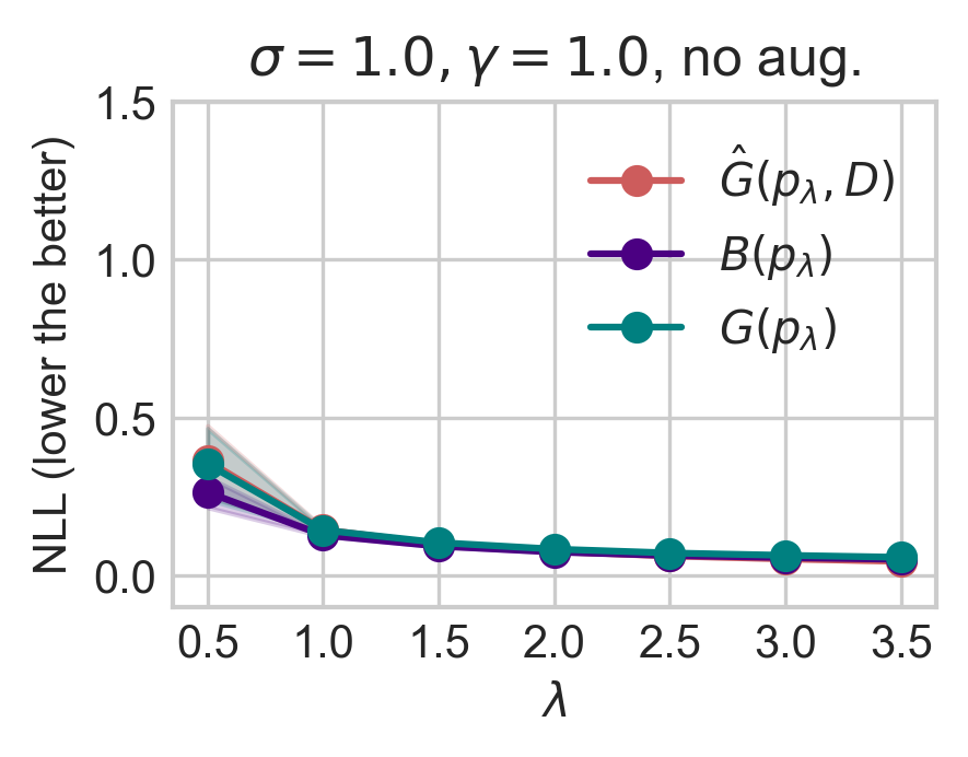
(a) Standard prior and standard softmax

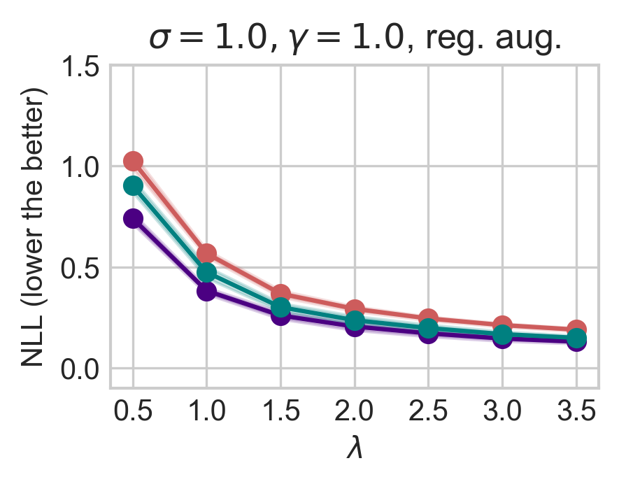
(b) Random crop and horizontal flip

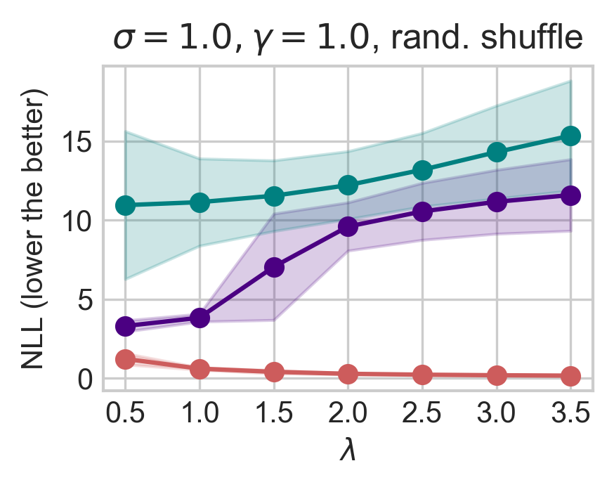
(c) Image pixels randomly shuffled

Figure 2.6: Experimental illustrations for the arguments in Section 2.6 using small CNN via SGLD on MNIST. We show similar results on Fashion-MNIST with small CNN and CIFAR-10(0) with ResNet-18 in Appendix LABEL:app:sec:experiment-approx. Figures 2.6(a) to 2.6(c) illustrate the arguments in Section 2.6. Figure 2.6(a) uses the standard prior ($\sigma=1$) and the standard softmax ($\gamma=1$) for the likelihood without applying DA. Figure 2.6(b) follows the setup as in Figure 2.6(a) but with standard DA applied, while Figure 2.6(c) uses fabricated DA. We report the training loss $\hat{G}(p_{\lambda},D)$ and the testing losses $B(p_{\lambda})$ and $G(p_{\lambda})$ from 10 samples of the small Convolutional neural network (CNN) via Stochastic Gradient Langevin Dynamics (SGLD). We show the mean and standard error across three different seeds. For additional experimental details, please refer to Appendix LABEL:app:sec:experiment-approx.

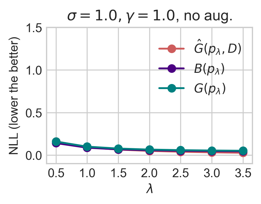
(a) Standard prior and standard softmax

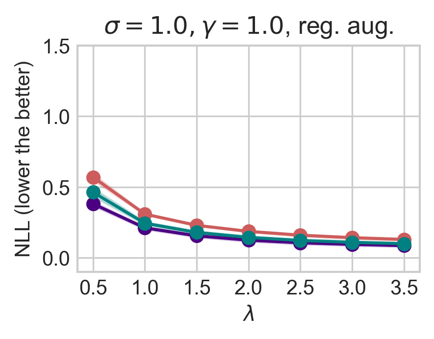
(b) Random crop and horizontal flip

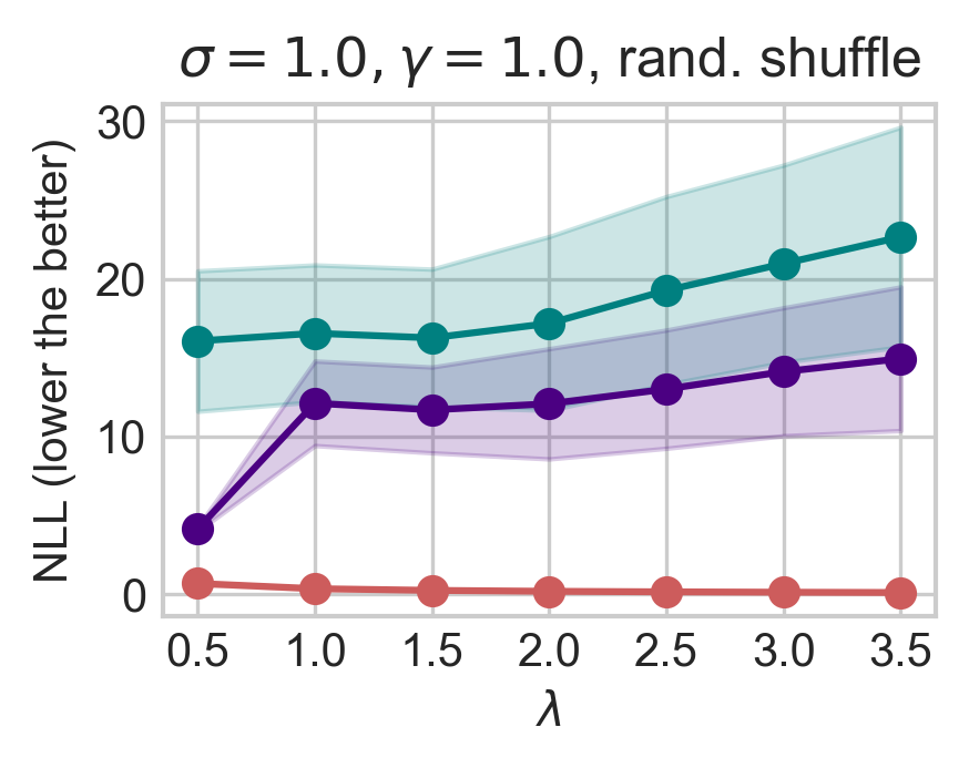
(c) Image pixels randomly shuffled

Figure 2.7: Experimental illustrations for the arguments in Section 2.6 using large CNN via SGLD on MNIST. We show similar results on Fashion-MNIST with large CNN and CIFAR-10(0) with ResNet-50 in Appendix LABEL:app:sec:experiment-approx. The experiment setup is similar to the setups in Figure 2.6 but with a large CNN. Please refer to Appendix LABEL:app:sec:experiment-approx for further details on the model.

Figure 2.6 clearly illustrates such situations. Figure 2.6(b) shows that, compared to Figure 2.6(a), the standard DA, which makes use of the invariances inherent in the data-generating distribution, induces a CPE on the Gibbs loss. Thus, the condition in Equation 2.15 holds by definition. On the other hand, Figure 2.6(c) uses a fabricated DA, where the same permutation is applied to the pixels of the images in the training dataset, which destroys low-level features present in the data-generating distribution. In this case, the derivative of the Gibb loss is positive, and Equation 2.15 holds in the opposite direction. These findings align perfectly with the explanations provided above, showing that DA induces a stronger underfitting.

2.6.2 Data augmentation and CPE on the Bayes loss

Now, we step aside of the Gibbs loss and focus back to the Bayes loss. The derivative of the Bayes loss at $\lambda=1$ can also be written as,

$$\frac{d}{d\lambda}B(p_{\lambda})_{|\lambda=1}=-\mathrm{COV}_{p_{\lambda=1}}\left(n\hat{L}(D,{\bm{\theta}}),S_{p_{\lambda=1}}({\bm{\theta}})\right)\,,$$ (2.16)

where for any posterior $\rho$, $S_{\rho}({\bm{\theta}})$ is a (negative) performance measure defined as

$$S_{\rho}({\bm{\theta}})=-\mathbb{E}_{\nu}\left[\frac{p({\bm{y}}|{\bm{x}},{\bm{\theta}})}{\mathbb{E}_{\rho}[p({\bm{y}}|{\bm{x}},{\bm{\theta}})]}\right]\,.$$ (2.17)

This function measures the relative performance of a model parameterized by ${\bm{\theta}}$ compared to the average performance of the models weighted by $\rho$. Such measure is conducted on samples from the data-generating distribution $\nu({\bm{y}},{\bm{x}})$. Specifically, if the model ${\bm{\theta}}$ outperforms the average, we have $S_{\rho}({\bm{\theta}})<-1$, and if the model performs worse than the average, we have $S_{p}({\bm{\theta}})>-1$ (i.e., the lower the better). The derivations of the above equations are given in Appendix 2.8.3.

According to Definition 2.1 and Equation 2.16, DA will induce a stronger CPE if and only if the following condition is satisfied:

$$\mathrm{COV}_{p_{\lambda=1}^{\text{\tiny{DA}}}}\left(n\hat{L}_{\text{\tiny{DA}}}(D,{\bm{\theta}}),S_{p_{\lambda=1}^{\text{\tiny{DA}}}}({\bm{\theta}})\right)>\mathrm{COV}_{p_{\lambda=1}}\left(n\hat{L}(D,{\bm{\theta}}),S_{p_{\lambda=1}}({\bm{\theta}})\right)\,.$$ (2.18)

The previous analysis on the Gibbs loss remains applicable in this context, with the use of $S_{\rho}({\bm{\theta}})$ as a metric for the expected performance on the true data-generating distribution instead of $L({\bm{\theta}})$. While these metrics are slightly different, it is reasonable to assume that the same arguments we presented to explain the CPE under data augmentation for the Gibbs loss also apply here. The theoretical analysis aligns with the behavior of the Bayes loss as depicted in Figure 2.6.

Finally, comparing Figure 2.6(b) with Figure 2.7(b), we also notice that using a larger neural network enables us to mitigate the CPE because we reduce the underfitting introduced by DA.

2.6.3 Related work of the data augmentation argument

The relation between data augmentation and CPE is an active topic of discussion (WRVS+20; IVHW21; NRBN+21; NGGA+22). Some studies suggest that CPE is an artifact of DA because turning off data augmentation is enough to eliminate the CPE (IVHW21; FGAO+22). Our study shows that this is much more than an artifact, as also argued in NGGA+22. As discussed, the (pseudo) log-likelihood induced by standard DA is a better proxy of the expected log-loss, as precisely defined by Equation 2.15 and Equation 2.18.

Some argue that when using DA, we are not using a proper likelihood function (IVHW21), which could be a problem. Recent works (NGGA+22) have developed principle likelihood functions that integrate DA-based approaches, hoping to remove CPE. However, they find that CPE still persists. Another widely accepted viewpoint regarding the interplay between the CPE and DA is that DA increases the effective sample size (IVHW21; NRBN+21): “intuitively, data augmentation increases the amount of data observed by the model, and should lead to higher posterior contraction” (IVHW21).

Our analysis provides a more nuance understanding of this interplay between CPE and DA. First, we show that, when the augmented data provide extra information about the data-generating process, there is a stronger CPE, as shown in Equations 2.15 and 2.18. This, in turn, leads to higher posterior concentration. But, we also show that higher posterior concentration in the context of non-meaningful DA does not improve performance; as discussed before, Figure 2.6(c) illustrates this situation. Using the analysis given in Section 2.4, we can also add that tempering the posterior under DA is again a way to define alternative Bayesian posteriors that addresses this stronger underfitting, i.e., they better fit the training data and improve generalization.

2.7 Conclusions and limitations

Our research contributes to understanding the cold posterior effect (CPE) and its implications for Bayesian deep learning in several ways. Firstly, we theoretically demonstrate that the presence of the CPE implies that the Bayesian posterior is underfitting. Secondly, by building on zeno2021why, we show that, in general, any tempered posterior can be considered as a proper Bayesian posterior with an alternative likelihood and prior distribution jointly parametrized by $T$, beyond merely the case of classification. Hence, fine-tuning the temperature parameter $T$ serves as an effective and theoretically sound approach to addressing the underfitting of the Bayesian posterior. Furthermore, we comprehensively discuss the interplay between several factors and CPE, including the use of approximate versus exact inference, model misspecification, and the size of the model and samples. Finally, our analysis in Section 2.6 reveals that data augmentation exacerbates the CPE by intensifying underfitting. This occurs because augmented data provides richer and more reliable information, enhancing the capacity for fitting.

Overall, our theoretical analysis underscores the significance of the CPE as an indicator of underfitting within the Bayesian framework and promotes the fine-tuning of the temperature $T$ in tempered posteriors as a principled approach to mitigate this issue. Furthermore, by dissecting the nature of the CPE and its effect on the Bayesian principle, our work aims to resolve ongoing debates and clarify the role of cold posteriors in enhancing the predictive performance of Bayesian deep learning models.

As a limitation of this work, we want to highlight that the characterization of CPE proposed here is defined only as the local change of Bayes loss at $\lambda=1$. This approach does not account for scenarios where significant decreases in Bayes loss at other $\lambda$ values might also indicate the presence of CPE. We believe that our theoretical analysis could be expanded to include these cases as well.

2.8 Appendix

2.8.1 Proofs for Section 2.3

In this section, we provide the proofs for Section 2.3 in the following order. We first prove the derivative of the empirical Gibbs loss in Proposition 2.1. Then, we show in Proposition 2.6 that for meaningful posteriors (depends on training data), the derivative won’t be zero. Before proving Proposition 2.2 and Theorem 2.3, we first provide Proposition 2.7, stating an alternative expression of the derivative of the Bayes loss. The proofs of Proposition 2.2 and Theorem 2.3 then follow from that.

2.8.1.1 Proof of Proposition 2.1

We first show a slightly more general result of $\frac{d}{d\lambda}\mathbb{E}_{p_{\lambda}}[f({\bm{\theta}})]$ for any function $f({\bm{\theta}})$ that is independent of $\lambda$. Recall that the posterior $p_{\lambda}({\bm{\theta}}|D)\propto p(D|{\bm{\theta}})^{\lambda}p({\bm{\theta}})$. With the fact that $\frac{d}{d\lambda}\left(p(D|{\bm{\theta}})^{\lambda}p({\bm{\theta}})\right)=\ln(p(D|{\bm{\theta}}))p(D|{\bm{\theta}})^{\lambda}p({\bm{\theta}})$, the derivative

$$\frac{d}{d\lambda}\mathbb{E}_{p_{\lambda}}[f({\bm{\theta}})]=\mathbb{E}_{p_{\lambda}}[\ln p(D|{\bm{\theta}})f({\bm{\theta}})]-\mathbb{E}_{p_{\lambda}}[\ln p(D|{\bm{\theta}})]\mathbb{E}_{p_{\lambda}}[f({\bm{\theta}})]=\mathrm{COV}_{p_{\lambda}}(\ln p(D|{\bm{\theta}}),f({\bm{\theta}}))\,,$$ (2.19)

where we denote $\mathrm{COV}(X,Y)$ as the covariance of $X$ and $Y$. Hence, the derivative of the empirical Gibbs loss

$$\frac{d}{d\lambda}\hat{G}(p_{\lambda},D) =\frac{d}{d\lambda}\mathbb{E}_{p_{\lambda}}[-\ln p(D|{\bm{\theta}})]$$

$$=\mathrm{COV}_{p_{\lambda}}(\ln p(D|{\bm{\theta}}),-\ln p(D|{\bm{\theta}}))$$

$$=-\mathbb{V}_{p_{\lambda}}(\ln p(D|{\bm{\theta}}))\,.$$

2.8.1.2 Proposition 2.6

Proposition 2.6.

For any $\lambda>0$ and $D\neq\varnothing$, if the tempered posterior $p_{\lambda}({\bm{\theta}}|D)\propto p(D|{\bm{\theta}})^{\lambda}p({\bm{\theta}})$ satisfies $\mathbb{V}_{p_{\lambda}}(\ln P(D|{\bm{\theta}}))=0$, then, $p_{\lambda}({\bm{\theta}}|D)=p({\bm{\theta}})$.

Proof.

First of all, note that the tempered posterior is defined as

$$p_{\lambda}({\bm{\theta}}|D)=\frac{p(D|{\bm{\theta}})^{\lambda}p({\bm{\theta}})}{\int_{\bm{\theta}}p(D|{\bm{\theta}})^{\lambda}p({\bm{\theta}})}\,.$$

Then,

$$\mathbb{V}_{p_{\lambda}}(\ln p(D|{\bm{\theta}}))=0\implies\int_{{\bm{\theta}}}p_{\lambda}({\bm{\theta}}|D)\left(\ln p(D|{\bm{\theta}})-\mathbb{E}_{p_{\lambda}}[\ln p(D|{\bm{\theta}})]\right)^{2}=0$$

Thus, for any ${\bm{\theta}}\in\text{supp}(p_{\lambda})$, it verifies that

$$\ln p(D|{\bm{\theta}})=\mathbb{E}_{p_{\lambda}}[\ln p(D|{\bm{\theta}})]\,.$$

That is, $\ln p(D|{\bm{\theta}})$ is constant in the support of $p_{\lambda}$. Let $c$ denote such constant, then

$$p_{\lambda}({\bm{\theta}}|D)=\frac{e^{c\lambda}p({\bm{\theta}})}{\int_{\bm{\theta}}e^{c\lambda}p({\bm{\theta}})}=\frac{e^{c\lambda}p({\bm{\theta}})}{e^{c\lambda}\int_{\bm{\theta}}p({\bm{\theta}})}=p({\bm{\theta}})\,.$$

$\square$

2.8.1.3 Proof of Proposition 2.2 and Theorem 2.3

In order to prove Proposition 2.2 and Theorem 2.3, we first show in Proposition 2.7 that the derivative of the Bayes loss of the tempered posterior $p_{\lambda}$ can be expressed by the difference between the empirical Gibbs loss of $\bar{p}_{\lambda}$ and the empirical Gibbs loss of $p_{\lambda}$.

Proposition 2.7.

The derivative of the Bayes loss of the tempered posterior $p_{\lambda}$ can be expressed by

$$\frac{d}{d\lambda}B(p_{\lambda})=\hat{G}(\bar{p}_{\lambda},D)-\hat{G}(p_{\lambda},D)\,.$$ (2.20)

Proof.

By definition,

$$\frac{d}{d\lambda}B(p_{\lambda})=\frac{d}{d\lambda}\mathbb{E}_{\nu}[{-\ln\mathbb{E}_{p_{\lambda}}[p({\bm{y}}|{\bm{x}},{\bm{\theta}})]}]=-\mathbb{E}_{\nu}\left[{\frac{d}{d\lambda}\ln\mathbb{E}_{p_{\lambda}}[p({\bm{y}}|{\bm{x}},{\bm{\theta}})]}\right],$$

where

$$\frac{d}{d\lambda}\ln\mathbb{E}_{p_{\lambda}}[p({\bm{y}}|{\bm{x}},{\bm{\theta}})]=\frac{\frac{d}{d\lambda}\mathbb{E}_{p_{\lambda}}[p({\bm{y}}|{\bm{x}},{\bm{\theta}})]}{\mathbb{E}_{p_{\lambda}}[p({\bm{y}}|{\bm{x}},{\bm{\theta}})]}=\frac{\mathrm{COV}_{p_{\lambda}}(\ln p(D|{\bm{\theta}}),p({\bm{y}}|{\bm{x}},{\bm{\theta}}))}{\mathbb{E}_{p_{\lambda}}[p({\bm{y}}|{\bm{x}},{\bm{\theta}})]}$$

due to Equation 2.19. By expanding the covariance, the above formula further equals to

$$\frac{\mathbb{E}_{p_{\lambda}}[\ln p(D|{\bm{\theta}})p({\bm{y}}|{\bm{x}},{\bm{\theta}})]-\mathbb{E}_{p_{\lambda}}[\ln p(D|{\bm{\theta}})]\mathbb{E}_{p_{\lambda}}[p({\bm{y}}|{\bm{x}},{\bm{\theta}})]}{\mathbb{E}_{p_{\lambda}}[p({\bm{y}}|{\bm{x}},{\bm{\theta}})]}$$

$$=\mathbb{E}_{\tilde{p}_{\lambda}}[\ln p(D|{\bm{\theta}})]-\mathbb{E}_{p_{\lambda}}[\ln p(D|{\bm{\theta}})]\,,$$

where the probability distribution $\tilde{p}_{\lambda}({\bm{\theta}}|D,({\bm{y}},{\bm{x}}))\propto p_{\lambda}({\bm{\theta}}|D)p({\bm{y}}|{\bm{x}},{\bm{\theta}})$. Put everything together, we have

$$\frac{d}{d\lambda}B(p_{\lambda})=\mathbb{E}_{p_{\lambda}}[\ln p(D|{\bm{\theta}})]-\mathbb{E}_{\nu}[\mathbb{E}_{\tilde{p}_{\lambda}}[\ln p(D|{\bm{\theta}})]]=\mathbb{E}_{p_{\lambda}}[\ln p(D|{\bm{\theta}})]-\mathbb{E}_{\bar{p}_{\lambda}}[\ln p(D|{\bm{\theta}})]\,,$$ (2.21)

where

$$\bar{p}_{\lambda}({\bm{\theta}}|D)=\mathbb{E}_{\nu}[\tilde{p}_{\lambda}({\bm{\theta}}|D,({\bm{y}},{\bm{x}}))]=\mathbb{E}_{\nu}\left[\frac{p_{\lambda}({\bm{\theta}}|D)p({\bm{y}}|{\bm{x}},{\bm{\theta}})}{\mathbb{E}_{p_{\lambda}}[p({\bm{y}}|{\bm{x}},{\bm{\theta}})]}\right].$$

The last equality is because

$$\mathbb{E}_{\nu}[\mathbb{E}_{\tilde{p}_{\lambda}}[\ln p(D|{\bm{\theta}})]] =\int_{({\bm{y}},{\bm{x}})}\nu({\bm{y}},{\bm{x}})\int_{{\bm{\theta}}}\tilde{p}_{\lambda}({\bm{\theta}}|D,({\bm{y}},{\bm{x}}))\ln p(D|{\bm{\theta}})\,d{\bm{\theta}}\,d({\bm{y}},{\bm{x}})$$

$$=\int_{\bm{\theta}}\int_{({\bm{y}},{\bm{x}})}\nu({\bm{y}},{\bm{x}})\tilde{p}_{\lambda}({\bm{\theta}}|D,({\bm{y}},{\bm{x}}))\,d({\bm{y}},{\bm{x}})\ln p(D|{\bm{\theta}})\,d{\bm{\theta}}$$

$$=\int_{\bm{\theta}}\mathbb{E}_{\nu}[\tilde{p}_{\lambda}({\bm{\theta}}|D,({\bm{y}},{\bm{x}}))]\ln p(D|{\bm{\theta}})\,d{\bm{\theta}}$$

$$=\mathbb{E}_{\bar{p}_{\lambda}}[\ln p(D|{\bm{\theta}})]\,.$$

The last expression in Equation 2.21 further equals to $\hat{G}(\bar{p}_{\lambda},D)-\hat{G}(p_{\lambda},D)$ by definition.   $\square$

2.8.1.3.1   Proof of Proposition 2.2

Note that for any distribution $\rho$, we have $\hat{G}(\rho,D):=\mathbb{E}_{\rho}{-\ln p(D|{\bm{\theta}})}\geq\min_{\bm{\theta}}-\ln p(D|{\bm{\theta}})$. On the other hand, Proposition 2.7 together with Definition 2.1 give that the CPE takes place if and only if

$$\frac{d}{d\lambda}B(p_{\lambda})_{|\lambda=1}=\hat{G}(\bar{p}_{\lambda=1},D)-\hat{G}(p_{\lambda=1},D)<0\,.$$

Therefore, it is not possible to have $\hat{G}(p_{\lambda=1},D)\not>\min_{\bm{\theta}}-\ln p(D|{\bm{\theta}})$ and, at the same time, $\hat{G}(\bar{p}^{\lambda=1},D)<\hat{G}(p_{\lambda=1},D)$ because $\hat{G}(\bar{p}^{\lambda=1},D)\geq\min_{\bm{\theta}}-\ln p(D|{\bm{\theta}})$.

2.8.1.3.2   Proof of Theorem 2.3

It’s easy to see from Proposition 2.7 that

$$\frac{d}{d\lambda}B(p_{\lambda})_{|\lambda=1}=\hat{G}(\bar{p}_{\lambda=1},D)-\hat{G}(p_{\lambda=1},D)=0$$

if and only if $\hat{G}(\bar{p}_{\lambda=1},D)=\hat{G}(p_{\lambda=1},D)$.

2.8.2 Proofs for Section 2.4

2.8.2.1 Proof of Proposition 2.4

First of all, by the definition in Equation 2.2, and assuming a data-independent prior $p({\bm{\theta}}|{\bm{X}})=p({\bm{\theta}})$, the tempered posterior is given by

$$p_{\lambda}({\bm{\theta}}|{\bm{X}},{\bm{Y}})\propto p({\bm{Y}}|{\bm{X}},{\bm{\theta}})^{\lambda}p({\bm{\theta}})\,,$$

where the tempered likelihood fully factorizes as $p({\bm{Y}}|{\bm{X}},{\bm{\theta}})^{\lambda}=\prod_{({\bm{y}},{\bm{x}})\in({\bm{Y}},{\bm{X}})}p({\bm{y}}|{\bm{x}},{\bm{\theta}})^{\lambda}$. Let a similar but ${\bm{y}}$-independent function $k({\bm{\theta}},{\bm{X}},\lambda)=\prod_{{\bm{x}}\in{\bm{X}}}\int p({\bm{y}}|{\bm{x}},{\bm{\theta}})^{\lambda}\,d{\bm{y}}$. Therefore, $p({\bm{Y}}|{\bm{X}},{\bm{\theta}})^{\lambda}p({\bm{\theta}})=\frac{p({\bm{Y}}|{\bm{X}},{\bm{\theta}})^{\lambda}}{k({\bm{\theta}},{\bm{X}},\lambda)}\left(k({\bm{\theta}},{\bm{X}},\lambda)p({\bm{\theta}})\right)$ , where we can let the new prior

$$q({\bm{\theta}}|{\bm{X}},\lambda)\propto p({\bm{\theta}})k({\bm{\theta}},{\bm{X}},\lambda)=p({\bm{\theta}})\prod_{{\bm{x}}\in{\bm{X}}}\int p({\bm{y}}|{\bm{x}},{\bm{\theta}})^{\lambda}\,d{\bm{y}}\,,$$

and the new posterior

$$q({\bm{Y}}|{\bm{X}},{\bm{\theta}},\lambda)=\frac{p({\bm{Y}}|{\bm{X}},{\bm{\theta}})^{\lambda}}{k({\bm{\theta}},{\bm{X}},\lambda)}=\frac{\prod_{({\bm{y}},{\bm{x}})\in({\bm{Y}},{\bm{X}})}p({\bm{y}}|{\bm{x}},{\bm{\theta}})^{\lambda}}{\prod_{{\bm{x}}\in{\bm{X}}}\int p({\bm{y}}|{\bm{x}},{\bm{\theta}})^{\lambda}\,d{\bm{y}}}=\prod_{({\bm{y}},{\bm{x}})\in({\bm{Y}},{\bm{X}})}q({\bm{y}}|{\bm{x}},{\bm{\theta}})\,.$$

2.8.2.2 Proof of Proposition 2.5

The proof is made using differential entropy, i.e. assuming continuous target values $\bm{y}$. The only assumption is that Leibniz integral rule holds for $q({\bm{y}}|{\bm{x}},{\bm{\theta}},\lambda)\ln q({\bm{y}}|{\bm{x}},{\bm{\theta}},\lambda))$, verifying that

$$\frac{d}{d\lambda}\int(q({\bm{y}}|{\bm{x}},{\bm{\theta}},\lambda)\ln q({\bm{y}}|{\bm{x}},{\bm{\theta}},\lambda))\ d{\bm{y}}=\int\frac{d}{d\lambda}(q({\bm{y}}|{\bm{x}},{\bm{\theta}},\lambda)\ln q({\bm{y}}|{\bm{x}},{\bm{\theta}},\lambda))\ d{\bm{y}}\,.$$

In the case of supervised classification problems, we adopt the Shanon entropy, where equality holds naturally

$$\frac{d}{d\lambda}\sum_{\bm{y}\in\mathcal{Y}}(q({\bm{y}}|{\bm{x}},{\bm{\theta}},\lambda)\ln q({\bm{y}}|{\bm{x}},{\bm{\theta}},\lambda))=\sum_{\bm{y}\in\mathcal{Y}}\frac{d}{d\lambda}(q({\bm{y}}|{\bm{x}},{\bm{\theta}},\lambda)\ln q({\bm{y}}|{\bm{x}},{\bm{\theta}},\lambda))\,.$$

From the definition of differential entropy, we got that

$$H(q({\bm{y}}|{\bm{x}},{\bm{\theta}},\lambda))=-\int q({\bm{y}}|{\bm{x}},{\bm{\theta}},\lambda)\ln q({\bm{y}}|{\bm{x}},{\bm{\theta}},\lambda)\ d{\bm{y}}\,.$$

Thus, taking derivative w.r.t. $\lambda$ and exchanging derivative and integral leads to the following expression

$$\frac{d}{d\lambda}H(q({\bm{y}}|{\bm{x}},{\bm{\theta}},\lambda)) =-\int\frac{d}{d\lambda}(q({\bm{y}}|{\bm{x}},{\bm{\theta}},\lambda)\ln q({\bm{y}}|{\bm{x}},{\bm{\theta}},\lambda))\ d{\bm{y}}$$

$$=-\int(\ln q({\bm{y}}|{\bm{x}},{\bm{\theta}},\lambda)+1)\frac{d}{d\lambda}q({\bm{y}}|{\bm{x}},{\bm{\theta}},\lambda)\ d{\bm{y}}\,.$$

Using that $\int\frac{d}{d\lambda}q({\bm{y}}|{\bm{x}},{\bm{\theta}},\lambda)d{\bm{y}}=\frac{d}{d\lambda}\int q({\bm{y}}|{\bm{x}},{\bm{\theta}},\lambda)d{\bm{y}}=0$, simplifies the expression as

$$\frac{d}{d\lambda}H(q({\bm{y}}|{\bm{x}},{\bm{\theta}},\lambda))=-\int\ln q({\bm{y}}|{\bm{x}},{\bm{\theta}},\lambda)\frac{d}{d\lambda}q({\bm{y}}|{\bm{x}},{\bm{\theta}},\lambda)\ d{\bm{y}}\,.$$

Let us consider now the second term inside the integral. Using the derivative of the quotient rule leads to the following:

$$\frac{d}{d\lambda}q({\bm{y}}|{\bm{x}},{\bm{\theta}},\lambda)$$

$$=\frac{d}{d\lambda}\frac{p({\bm{y}}|{\bm{x}},{\bm{\theta}})^{\lambda}}{\int p({\bm{y}}|{\bm{x}},{\bm{\theta}})^{\lambda}\ d{\bm{y}}}$$

$$=\frac{p({\bm{y}}|{\bm{x}},{\bm{\theta}})^{\lambda}\ln p({\bm{y}}|{\bm{x}},{\bm{\theta}})}{\int p({\bm{y}}|{\bm{x}},{\bm{\theta}})^{\lambda}\ d{\bm{y}}}-\frac{p({\bm{y}}|{\bm{x}},{\bm{\theta}})^{\lambda}\int p({\bm{y}}|{\bm{x}},{\bm{\theta}})^{\lambda}\ln p({\bm{y}}|{\bm{x}},{\bm{\theta}})\ d{\bm{y}}}{(\int p({\bm{y}}|{\bm{x}},{\bm{\theta}})^{\lambda}\ d{\bm{y}})^{2}}\,.$$

Where, using the definition of $q({\bm{y}}|{\bm{x}},{\bm{\theta}},\lambda)$, we got that

$$\frac{p({\bm{y}}|{\bm{x}},{\bm{\theta}})^{\lambda}\ln p({\bm{y}}|{\bm{x}},{\bm{\theta}})}{\int p({\bm{y}}|{\bm{x}},{\bm{\theta}})^{\lambda}\ d{\bm{y}}}=q({\bm{y}}|{\bm{x}},{\bm{\theta}},\lambda)\ln p({\bm{y}}|{\bm{x}},{\bm{\theta}})\,,$$

and

$$\frac{p({\bm{y}}|{\bm{x}},{\bm{\theta}})^{\lambda}\int p({\bm{y}}|{\bm{x}},{\bm{\theta}})^{\lambda}\ln p({\bm{y}}|{\bm{x}},{\bm{\theta}})\ d{\bm{y}}}{(\int p({\bm{y}}|{\bm{x}},{\bm{\theta}})^{\lambda}\ d{\bm{y}})^{2}}$$

$$=q({\bm{y}}|{\bm{x}},{\bm{\theta}},\lambda)\int q({\bm{y}}|{\bm{x}},{\bm{\theta}},\lambda)\ln p({\bm{y}}|{\bm{x}},{\bm{\theta}})\ d{\bm{y}}$$

$$=q({\bm{y}}|{\bm{x}},{\bm{\theta}},\lambda)\mathbb{E}_{q}[\ln p({\bm{y}}|{\bm{x}},{\bm{\theta}})]\,.$$

As a result, we got that

$$\int\ln q({\bm{y}}|{\bm{x}},{\bm{\theta}},\lambda)\frac{d}{d\lambda}q({\bm{y}}|{\bm{x}},{\bm{\theta}},\lambda)\ d{\bm{y}}$$

$$=\mathbb{E}_{q}[\ln p({\bm{y}}|{\bm{x}},{\bm{\theta}})\ln q({\bm{y}}|{\bm{x}},{\bm{\theta}},\lambda)]-\mathbb{E}_{q}[\ln q({\bm{y}}|{\bm{x}},{\bm{\theta}},\lambda)]\mathbb{E}_{q}[\ln p({\bm{y}}|{\bm{x}},{\bm{\theta}})]$$

Using $q({\bm{y}}|{\bm{x}},{\bm{\theta}},\lambda)$ definition again:

$$\int\ln q({\bm{y}}|{\bm{x}},{\bm{\theta}},\lambda)\frac{d}{d\lambda}q({\bm{y}}|{\bm{x}},{\bm{\theta}},\lambda)\ d{\bm{y}}$$

$$=\mathbb{E}_{q}[\ln p({\bm{y}}|{\bm{x}},{\bm{\theta}})\ln\frac{p({\bm{y}}|{\bm{x}},{\bm{\theta}})^{\lambda}}{\int p({\bm{y}}|{\bm{x}},{\bm{\theta}})^{\lambda}}]-\mathbb{E}_{q}[\ln\frac{p({\bm{y}}|{\bm{x}},{\bm{\theta}})^{\lambda}}{\int p({\bm{y}}|{\bm{x}},{\bm{\theta}})^{\lambda}}]\mathbb{E}_{q}[\ln p({\bm{y}}|{\bm{x}},{\bm{\theta}})]$$

Where, expanding the logarithms the denominators cancel each other, leading to

$$\int\ln q({\bm{y}}|{\bm{x}},{\bm{\theta}},\lambda)\frac{d}{d\lambda}q({\bm{y}}|{\bm{x}},{\bm{\theta}},\lambda)\ d{\bm{y}}$$

$$=\mathbb{E}_{q}[\ln p({\bm{y}}|{\bm{x}},{\bm{\theta}})\ln p({\bm{y}}|{\bm{x}},{\bm{\theta}})^{\lambda}]-\mathbb{E}_{q}[\ln p({\bm{y}}|{\bm{x}},{\bm{\theta}})^{\lambda}]\mathbb{E}_{q}[\ln p({\bm{y}}|{\bm{x}},{\bm{\theta}})]$$

$$=\lambda\mathbb{V}(\ln p({\bm{y}}|{\bm{x}},{\bm{\theta}}))\geq 0$$

As a result, the entropy is negative.

2.8.3 Proofs for Section 2.6

2.8.3.1 Proof of Equation 2.14

Note that

$$\frac{d}{d\lambda}G(p_{\lambda})=\frac{d}{d\lambda}\mathbb{E}_{p_{\lambda}}[L({\bm{\theta}})]=\mathrm{COV}_{p_{\lambda}}(\ln p(D|{\bm{\theta}}),L({\bm{\theta}}))=\mathrm{COV}_{p_{\lambda}}(-\hat{L}(D,{\bm{\theta}}),L({\bm{\theta}})),$$

where the second equality is by applying Equation 2.19. By taking $\lambda=1$, we obtain the desired derivative.

2.8.3.2 Proof of Equation 2.16

Recall from the proof of Theorem 2.7 that

$$\frac{d}{d\lambda}B(p_{\lambda})=\mathbb{E}_{p_{\lambda}}[\ln p(D|{\bm{\theta}})]-\mathbb{E}_{\bar{p}_{\lambda}}[\ln p(D|{\bm{\theta}})]=\mathbb{E}_{\bar{p}_{\lambda}}[\hat{L}(D,{\bm{\theta}})]-\mathbb{E}_{p_{\lambda}}[\hat{L}(D,{\bm{\theta}})],$$

where $\bar{p}_{\lambda}({\bm{\theta}}|D)=\mathbb{E}_{\nu}\left[\tilde{p}_{\lambda}({\bm{\theta}}|D,({\bm{y}},{\bm{x}}))\right]$ (Equation 2.6), and $\tilde{p}_{\lambda}({\bm{\theta}}|D,({\bm{y}},{\bm{x}}))\propto p_{\lambda}({\bm{\theta}}|D)p({\bm{y}}|{\bm{x}},{\bm{\theta}})$ is the distribution obtained by updating the posterior $p_{\lambda}$ with one new sample $({\bm{y}},{\bm{x}})$. Therefore,

$$\mathbb{E}_{\bar{p}_{\lambda}}[\hat{L}(D,{\bm{\theta}})]=\mathbb{E}_{\nu}\mathbb{E}_{\tilde{p}_{\lambda}}[\hat{L}(D,{\bm{\theta}})]=\mathbb{E}_{\nu}\left[\mathbb{E}_{p_{\lambda}}\left[\frac{p({\bm{y}}|{\bm{x}},{\bm{\theta}})}{\mathbb{E}_{p_{\lambda}}[p({\bm{y}}|{\bm{x}},{\bm{\theta}})]}\hat{L}(D,{\bm{\theta}})\right]\right].$$

By Fubini’s theorem, the above formula further equals to

$$\mathbb{E}_{p_{\lambda}}\left[\mathbb{E}_{\nu}\left[\frac{p({\bm{y}}|{\bm{x}},{\bm{\theta}})}{\mathbb{E}_{p_{\lambda}}[p({\bm{y}}|{\bm{x}},{\bm{\theta}})]}\hat{L}(D,{\bm{\theta}})\right]\right] =\mathbb{E}_{p_{\lambda}}\left[\mathbb{E}_{\nu}\left[\frac{p({\bm{y}}|{\bm{x}},{\bm{\theta}})}{\mathbb{E}_{p_{\lambda}}[p({\bm{y}}|{\bm{x}},{\bm{\theta}})]}\right]\hat{L}(D,{\bm{\theta}})\right]$$

$$=\mathbb{E}_{p_{\lambda}}\left[-S_{p_{\lambda}}({\bm{\theta}})\cdot\hat{L}(D,{\bm{\theta}})\right].$$

On the other hand, since

$$\mathbb{E}_{p_{\lambda}}[-S_{p_{\lambda}}({\bm{\theta}})]=\mathbb{E}_{p_{\lambda}}\left[\mathbb{E}_{\nu}\left[\frac{p({\bm{y}}|{\bm{x}},{\bm{\theta}})}{\mathbb{E}_{p_{\lambda}}[p({\bm{y}}|{\bm{x}},{\bm{\theta}})]}\right]\right]=\mathbb{E}_{\nu}\left[\mathbb{E}_{p_{\lambda}}\left[\frac{p({\bm{y}}|{\bm{x}},{\bm{\theta}})}{\mathbb{E}_{p_{\lambda}}[p({\bm{y}}|{\bm{x}},{\bm{\theta}})]}\right]\right]=1\,,$$

we have

$$\mathbb{E}_{p_{\lambda}}[\hat{L}(D,{\bm{\theta}})]=\mathbb{E}_{p_{\lambda}}[\hat{L}(D,{\bm{\theta}})]\mathbb{E}_{p_{\lambda}}[-S_{p_{\lambda}}({\bm{\theta}})]\,.$$

By putting them altogether,

$$\frac{d}{d\lambda}B(p_{\lambda}) =\mathbb{E}_{p_{\lambda}}\left[-S_{p_{\lambda}}({\bm{\theta}})\cdot\hat{L}(D,{\bm{\theta}})\right]-\mathbb{E}_{p_{\lambda}}[\hat{L}(D,{\bm{\theta}})]\mathbb{E}_{p_{\lambda}}[-S_{p_{\lambda}}({\bm{\theta}})]$$

$$=-\mathrm{COV}\left(\hat{L}(D,{\bm{\theta}}),S_{p_{\lambda}}({\bm{\theta}})\right)\,.$$

2.8.4 Experiment details for Bayesian linear regression on synthetic data with exact inference

In this section we detail the settings of the toy experiment using synthetic data and exact Bayesian linear regression in Figures 2.2 and 2.3. We also show extra results of the derivative of Gibbs loss and Bayes loss w.r.t to $\lambda$ approximated by samples.

To begin, we will outline the data-generating process for the synthetic data used in the experiment shown in Figures 2.2 and 2.3 and Figures LABEL:fig:blr_appendix and LABEL:fig:blr2_appendix. We sample $x$ uniformly from the $[-1,1]$ interval and pass it through a Fourier transformation to construct the input of the data. That is, for a sampled $x$, the input ${\bm{x}}$ is constructed by a 10-dimensional Fourier basis function $\text{ϕ}\text{(x)=[g\_1(x), …, g\_K(x)]^T}for\text{K=10},wherethebasisfunctionsaredefinedasfollows:\text{g\_1(x)=}{\displaystyle \frac{\text{1}}{\sqrt{\text{2}\text{π}}}},andforotheroddvaluesof\text{k}\text{,}\text{g\_k(x)=}{\displaystyle \frac{\text{1}}{\sqrt{\text{π}}}}\text{sin(kx)},whereasforevenvaluesof\text{k}\text{,}\text{g\_k(x)=}{\displaystyle \frac{\text{1}}{\sqrt{\text{π}}}}\text{cos(kx)}.Thedistributionoftheoutput\text{y∈}\text{R}givenaninputx,denotedas\text{ν}\text{(y|}x\text{)},followsaNormaldistributionwithmean\text{1^T}xandvariance\text{1.0},where\text{1}isanall-onesvector.Thatis,\text{ν}\text{(y|}x\text{)=}\text{N}\text{(1^T}x\text{,1.0)}.\text{Figure 2.8Figure 2.82.8Figure 2.8(a)2.8(a)2.8(a)(a)Nolikelihoodorpriormisspecification(a)Nolikelihoodorpriormisspecification(b)2.8(b)2.8(b)(b)Likelihood}$