Likelihood-Free Inference and Hierarchical Data Assimilation for Geological Carbon Storage

Abstract

Data assimilation will be essential for the management and expansion of geological carbon storage operations. In traditional data assimilation approaches a fixed set of geological hyperparameters, such as mean and standard deviation of log-permeability, is often assumed. Such hyperparameters, however, may be highly uncertain in practical CO₂ storage applications. In this study, we develop a hierarchical data assimilation framework for carbon storage that treats hyperparameters as uncertain variables characterized by hyperprior distributions. To deal with the computationally intractable likelihood function in hyperparameter estimation, we apply a likelihood-free (or simulation-based) inference algorithm, specifically sequential Monte Carlo-based approximate Bayesian computation (SMC-ABC), to draw independent posterior samples of hyperparameters given dynamic monitoring-well data. In the second step we use an ensemble smoother with multiple data assimilation (ESMDA) procedure to provide posterior realizations of grid-block permeability. To reduce computational costs, a 3D recurrent R-U-Net deep-learning-based surrogate model is applied for forward function evaluations. The accuracy of the surrogate model is established through comparisons to high-fidelity simulation results. A rejection sampling (RS) procedure for data assimilation is applied to provide reference posterior results. Detailed data assimilation results from SMC-ABC-ESMDA are compared to those from the reference RS method. These include marginal posterior distributions of hyperparameters, pairwise posterior samples, and history matching results for pressure and saturation at the monitoring location. Close agreement is achieved with ‘converged’ RS results, for two synthetic true models, in all quantities considered. Importantly, the SMC-ABC-ESMDA procedure provides speedup of 1–2 orders of magnitude relative to RS for the two cases.

[a]Department of Energy Science and Engineering, Stanford University, Stanford, CA 94305, USA

1 Introduction

Geological carbon storage offers a potential means to significantly reduce $\mathrm{CO}_{2}$ emissions to the atmosphere. Such operations, however, typically involve substantial uncertainty due to the limited information available regarding storage aquifer properties. This uncertainty can be reduced by applying data assimilation (or history matching) procedures, which act to provide geological realizations that give flow simulation results in approximate agreement with observed data. A common issue in traditional data assimilation frameworks, however, is the challenge of determining appropriate values for the relevant hyperparameters (also referred to as scenario parameters or metaparameters). Examples of these hyperparameters are the mean and standard deviation of porosity and permeability, permeability anisotropy ratio, correlation lengths, etc. Because inappropriate assumptions regarding hyperparameter values can lead to implausible posterior realizations and biased predictions [25], it is important to include hyperparameter estimation in the data assimilation procedure.

In this paper, we present a hierarchical data assimilation framework to estimate hyperparameters and grid-block permeability values given dynamic monitoring-well data. In contrast to many traditional data assimilation approaches, we treat the hyperparameters as uncertain. Our specific procedure involves a sequential Monte Carlo-based approximate Bayesian computation (SMC-ABC) method for hyperparameter estimation, followed by an ensemble smoother with multiple data assimilation (ESMDA) to provide posterior realizations of grid-block permeability. These treatments require a substantial number of function evaluations. We thus apply a deep-learning-based flow simulation surrogate model [39, 16] in place of a high-fidelity numerical simulator. The use of this surrogate model also enables us to compare data assimilation results from our method with those from the much more computationally intensive rejection sampling procedure.

Data assimilation has been extensively studied and applied in subsurface flow settings. Ensemble Kalman-based approaches, such as ensemble Kalman filter (EnKF) [12] and ensemble smoother with multiple data assimilation (ESMDA) [11], are widely used for oil reservoir simulation and for geological carbon storage (GCS) modeling. In the context of GCS, ensemble-based methods have been applied, for example, for the detection of potential leakage pathways [15] and for uncertainty reduction in risk assessment studies [8]. Different types of measurements have been considered with ensemble-based methods. These include time-lapse seismic surveys [22], microseismic events [18], and InSAR surface displacement data [37]. The large volume of observed data has also stimulated the application of more advanced techniques for dimension reduction and efficient parameterization [22, 37]. The above-mentioned studies did not, however, consider hyperparameter uncertainty.

Deep-learning-based surrogate models have been actively developed for GCS applications. Our discussion on this topic will be brief, however, as the development of a surrogate model is not the focus of this work. A range of network architectures has been used for GCS modeling. These include the Recurrent Residual U-Net [40], Wide ResNet [38], Fourier Neural Operators [45, 32], and Transformer U-Net [32]. The use of these surrogate models has enabled formal, though computationally demanding, data assimilation approaches to be applied for carbon storage problems. Tang et al. [39], for example, used their 3D recurrent R-U-Net surrogate model with a rejection sampling method to history match coupled flow and geomechanics problems. Han et al. [16] extended the recurrent R-U-Net model and incorporated it into a Markov chain Monte Carlo (MCMC) history matching procedure in which hyperparameter uncertainty was also considered.

Compared to traditional data assimilation (with assumed/fixed hyperparameters), less effort has been directed toward the hierarchical Bayesian inference problem [14] involving the joint estimation of posterior hyperparameters and geological realizations. One of the first approaches to address this issue was the quasi-linear geostatistical theory by Kitanidis [21]. Based on this work, Zhao and Luo [47] proposed an iterative method to correct the prior hyperparameters. These procedures rely on linearization and thus have limitations for strongly nonlinear problems. MCMC has also been used for hierarchical Bayesian problems in subsurface settings [17, 29, 46, 16]. Most MCMC approaches are expensive, however, and they do not naturally parallelize. Some of these methods involve a hierarchically noncentered parameterization in which hyperparameters and latent variables are a priori independent [27]. Such a parameterization is also applicable for ensemble Kalman-based data assimilation when the augmented parameter space is assumed to be Gaussian [7, 24]. The above-mentioned studies using a noncenterd parameterization rely on parameter covariance matrix factorization and latent Gaussian models. These factors introduce additional challenges to data assimilation in 3D subsurface problems.

The rigorous calculation of the likelihood of observed data given the hyperparameters is computationally intractable. This is because the likelihood function corresponds to an integral over all possible geomodel realizations. Various treatments have been introduced to address this issue. Friedli et al. [13] used a correlated pseudo-marginal Metropolis-Hastings algorithm to estimate the marginal posterior distributions of geostatistical hyperparameters given geophysical data. Wang et al. [44] presented a machine learning-based inversion method to estimate the posterior distributions of hydrological hyperparameters. The problem of an intractable likelihood function also arises in other fields, such as population genetics [5], ecology [3], and cosmology [1], and this has motivated the development of various likelihood-free inference algorithms. These can be categorized into two broad classes, as we now discuss.

The first class of methods uses the forward simulator directly during the inference process. A widely used method is approximate Bayesian computation (ABC) [34]. Efficient approaches have been developed by combining ABC with MCMC [23] and with sequential Monte Carlo (SMC) methods [35, 41, 4]. The second class of likelihood-free methods uses the simulator to train neural conditional density estimators to provide the likelihood [42] or posterior [26] of hyperparameters. There have only been a few studies and applications of likelihood-free inference methods in subsurface settings [9, 43]. To our knowledge, these methods have not yet been considered within the context of GCS.

Our goal in this paper is to develop and apply a hierarchical data assimilation framework for geological carbon storage problems. Specifically, we implement a sequential Monte Carlo-based approximate Bayesian computation (SMC-ABC) method to calibrate the hyperparameters, followed by ESMDA to provide posterior realizations of grid-block permeability. Our hierarchical framework is quite different from existing approaches used for data assimilation in GCS. Specifically, samples from SMC-ABC are independent and thus the computations are inherently parallel. This represents a significant advantage over MCMC methods. In addition, the SMC-ABC approach is fundamentally global. It thus avoids getting ‘stuck’ in local modes of the parameter space, and it does not require a burn-in period. Finally, the proposed procedure does not require a noncentered parameterization. We evaluate the performance of the hierarchical procedure for two synthetic ‘true’ models. The rejection sampling (RS) method is used as a reference for the posterior hyperparameter distributions. The substantial efficiency gains provided by the hierarchical procedure relative to the rigorous RS procedure are quantified.

This paper proceeds as follows. In Section 2, we briefly describe the problem setup and the recurrent R-U-Net surrogate model used in this work. Comparisons of surrogate model predictions to high-fidelity simulation results will also be presented. Next, in Section 3, we develop the hierarchical data assimilation procedure involving SMC-ABC followed by ESMDA. An overview of the RS algorithm is also provided. Detailed data assimilation results for two synthetic true models, including quantitative comparisons to RS, are provided in Section 4. We conclude with a summary and suggestions for future work in Section 5.

2 Simulation Setup and Surrogate Model

In this section, we first describe the geological model and simulation specifications. The surrogate model and the training procedure are then discussed. Comparisons of surrogate model predictions to reference simulation results are provided.

2.1 Geomodel and simulation parameters

The overall domain considered in the flow simulations, shown in Fig. 1, includes a central storage aquifer and an extensive surrounding region that provides pressure support. The full system is of size 72 km $\times$ 72 km $\times$ 120 m, and the storage aquifer region is 7.2 km $\times$ 7.2 km $\times$ 120 m. The overall system is represented on a grid containing 70 $\times$ 70 $\times$ 12 cells. The storage aquifer grid is 60 $\times$ 60 $\times$ 12. The grid is uniform in the storage aquifer region and nonuniform, with increasing cell dimensions as we move away from the storage aquifer, in the surrounding region. The aquifer is characterized by a heterogeneous permeability field. Porosity is considered to be constant but uncertain. The surrounding region is assigned a constant permeability of 30 md and a constant porosity of 0.2.

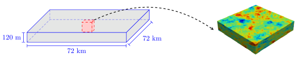
Figure 1: Full simulation domain (left), and central storage aquifer with heterogeneous permeability field (right).

Permeability realizations of the storage aquifer are constructed using sequential Gaussian simulation in the geostatistical software library GSLIB [10]. The spatial correlation of the permeability field is described using an exponential variogram model. The correlation length (or variogram range) is considered to be an uncertain hyperparameter. The other uncertain hyperparameters considered in this work are the mean and standard deviation of log-permeability, permeability anisotropy ratio, and storage aquifer porosity. The priors of these hyperparameters, referred to as hyperpriors, are all assumed to follow the uniform distributions given in Table 1. Other distributions could also be used in our formulation.

Table 1: Hyperparameters and hyperpriors

Parameters	Prior distribution
Mean of log-permeability, $\mu_{\log k}$	$\mu_{\log k}\sim$ $U$(2.5, 4.5)
Standard deviation of log-permeability, $\sigma_{\log k}$	$\sigma_{\log k}\sim$ $U$(0.5, 2)
Permeability anisotropy ratio, $a_{r}$	$\log_{10}a_{r}$ $\sim$ $U$(-2, 0)
Horizontal correlation length, $l_{h}$	$l_{h}\sim$ $U$(5, 20)
Constant porosity, $\phi$	$\phi$ $\sim$ $U$(0.13, 0.23)

With the geomodel realizations as input, we perform numerical flow simulation to obtain pressure and saturation fields at a set of time steps. In the simulations, a single fully-penetrating vertical injector is placed in the middle of the storage aquifer. A monitoring well, as shown in Fig. 2, is located near the injector. We specify a constant $\mathrm{CO}_{2}$ injection rate of 1 Mt/year for 30 years. The aquifer is of initial pressure 15.5 MPa in the top layer. The temperature is constant at 55 $\mathrm{\SIUnitSymbolCelsius}$. Relative permeability hysteresis, as shown in Fig. 3(a), is included in the model. The Leverett J-function is used to calculate heterogeneous capillary pressure based on permeability and porosity. The simulation model does not include any geochemical reactions. All flow simulations are performed using the ECLIPSE simulator with the CO2STORE option [31].

Figure 2: Locations of the injection well and monitoring well in the storage aquifer.

(a) Relative permeabilities with hysteresis (from [6])

(b) Capillary pressure curve (from [36])

Figure 3: $\text{CO}_{2}$–brine two-phase flow functions. Curve in (b) is for porosity of 0.2 and permeability of 10 md.

2.2 Surrogate model training and evaluation

The SMC-ABC-ESMDA methodology developed in this work requires ${\mathcal{O}}(10^{5})$ function evaluations for data assimilation in the examples considered. This method will be compared to a reference rejection sampling procedure that requires ${\mathcal{O}}(10^{6}-10^{7})$ function evaluations. Given these large simulation demands, it is clearly beneficial to replace the numerical flow simulator with a fast surrogate model for the great majority of function evaluations. A number of accurate and effective such models have been developed (as discussed in the Introduction). Here we will apply an existing framework that is well-suited for our application.

In this work we use the 3D recurrent R-U-Net model presented in [40, 39, 16]. This model involves convolutional and recurrent (convLSTM) networks, and acts to map the input geomodel to pressure and saturation fields at a specified set of time steps. Separate networks are trained for pressure and saturation variables. The accuracy of recurrent R-U-Net surrogate model predictions has been assessed for $\mathrm{CO}_{2}$ storage problems in [39, 16], where it was shown to provide results in close agreement (within a few percent) with reference numerical simulation results.

The surrogate model is trained using simulation results for a set of realizations sampled from the prior. This entails drawing hyperparameter samples (from the distributions given in Table 1) and then applying GSLIB to generate geological realizations. Here we construct and simulate 2000 prior geomodels, which we denote as $\mathbf{m}_{i}$, $i=1,\ldots,2000$. Storage aquifer pressure and saturation fields at time $t=1$, 4, 7, 10, 13, 16, 20, 23, 26 and 30 years are saved. The networks are then trained (i.e., optimal network parameters are determined) such that the difference between predicted and simulated results is minimized. For detailed descriptions of the network architecture and training procedure, please refer to [39, 16].

We now quantify the prediction errors in the trained networks for pressure and saturation. A set of 500 new geomodels (referred to as the test set) is generated, using the same sampling procedure described above, and then simulated. The relative errors in pressure and saturation, $\delta_{p}^{i}$ and $\delta_{S}^{i}$, for each test-case sample $i$, are defined as follows:

$$\delta_{p}^{i}=\frac{1}{n_{s}n_{t}}\sum_{j=1}^{n_{s}}\sum_{t=1}^{n_{t}}\frac{|(\hat{p}_{s})_{i,j}^{t}-(p_{s})_{i,j}^{t}|}{(p_{s})_{i,\mathrm{max}}^{t}-(p_{s})_{i,\mathrm{min}}^{t}},$$ (1)

$$\delta_{S}^{i}=\frac{1}{n_{s}n_{t}}\sum_{j=1}^{n_{s}}\sum_{t=1}^{n_{t}}\frac{|(\hat{S}_{s})_{i,j}^{t}-(S_{s})_{i,j}^{t}|}{(S_{s})_{i,j}^{t}+\epsilon},$$ (2)

where $i,j,t$ are the number index for test case, grid block, and time step, respectively, ${n_{s}}=43,200$ is the number of grid blocks in the storage aquifer, and $n_{t}=10$ is the number of time steps considered in the surrogate models. The quantities $\hat{p}_{s}$ and $\hat{S}_{s}$ are pressure and $\mathrm{CO}_{2}$ saturation predictions provided by the surrogate model, $p_{s}$ and $S_{s}$ are analogous predictions from ECLIPSE, $(p_{s})_{i,\mathrm{max}}^{t}$ and $(p_{s})_{i,\mathrm{min}}^{t}$ are the maximum and minimum pressure in test case $i$ at time step $t$, and $\epsilon$ = 0.025 is a constant included to avoid division by zero or near-zero values.

Histograms for pressure and saturation errors computed using Eqs. 1 and 2 are shown in Fig. 4. The mean relative errors for pressure and saturation are 0.8% and 2.3%, respectively. Saturation error is larger than pressure error due to the more complex local dynamics and sharp fronts associated with the saturation fields. The errors observed in Fig. 4 are smaller than those in previous studies [16, 39], presumably because our model involves only a single injection well.

(a) Relative error for pressure

(b) Relative error for $\text{CO}_{2}$ saturation

Figure 4: Histograms for relative errors for the test set.

We next assess the performance of the surrogate model from two other perspectives. First, we compare the ensemble statistics for particular grid blocks intersected by the monitoring well. Results of this type are important because these quantities are used directly in the history matching procedure. Time-series for pressure, in layers 1 and 6 at the monitoring well location, are shown in Fig. 5. Results are presented in terms of $\mathrm{P}_{10}$, $\mathrm{P}_{50}$ and $\mathrm{P}_{90}$ (percentile) responses. Close agreement between the two sets of results is clearly observed, demonstrating the accuracy of the surrogate model for these local quantities.

We next compare field-scale solutions for $\mathrm{CO}_{2}$ saturation at the end of the injection period (30 years). We apply the $k$-means and $k$-medoids clustering procedure described in [33, 19] to select distinct (representative) saturation fields. These fields are shown in Fig. 6, with simulation results in the upper row and surrogate predictions in the lower row. Note the different plume shapes and extents between the four models. The surrogate predictions are visually close to the reference simulation results in all cases, consistent with the errors in Fig. 4(b). In total, the results presented in Figs. 4, 5 and 6 demonstrate the accuracy of the surrogate model and highlight its applicability for use in data assimilation.

(a) Pressure in layer 1 (top of model)

(b) Pressure in layer 6

Figure 5: Comparison of pressure ensemble statistics from the surrogate model (red dashed curves) and simulation results (black solid curves) at grid blocks intersected by the monitoring well. The lower, middle and upper curves are $\mathrm{P}_{10}$, $\mathrm{P}_{50}$ and $\mathrm{P}_{90}$ results among the 500 test cases.

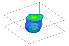
(a)

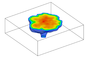
(b)

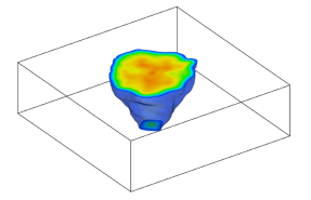
(c)

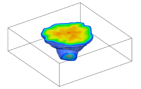
(d)

(e)

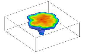
(f)

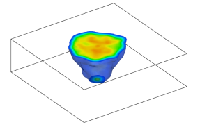
(g)

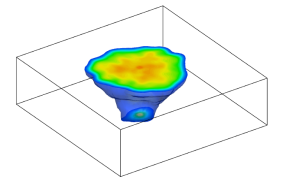
(h)

Figure 6: $\text{CO}_{2}$ saturation at 30 years from ECLIPSE simulation (upper row) and the recurrent R-U-Net surrogate model (lower row) for four representative realizations.

3 Hierarchical Data Assimilation

We begin this section with a description of the overall workflow for the hierarchical data assimilation procedure. The key algorithm used in our procedure, sequential Monte Carlo-based approximate Bayesian computation (SMC-ABC), is described in detail. Ensemble smoother with multiple data assimilation (ESMDA) is also discussed. Rejection sampling (RS), used as a reference, is then presented.

3.1 Overall workflow

Many traditional data assimilation procedures involve a fixed set of hyperparameters. In such cases, the grid-block permeabilities or porosities are typically the model parameters to be estimated. These high-dimensional discrete parameters can be inferred using Bayes’ law:

$$p(\mathbf{m}|\mathbf{d}_{\text{obs}})=\frac{p({\mathbf{m}})p(\mathbf{d}_{\text{obs}}|\mathbf{m})}{p(\mathbf{d}_{\text{obs}})},$$ (3)

where $\mathbf{m}$ represents the discretized model parameters, $\mathbf{d}_{\text{obs}}$ denotes the observed data, $p({\mathbf{m}})$ is the prior density, $p(\mathbf{d}_{\text{obs}}|\mathbf{m})$ is the likelihood function, $p(\mathbf{m}|\mathbf{d}_{\text{obs}})$ is the posterior density, and $p(\mathbf{d}_{\text{obs}})$ is the evidence. The hyperparameters do not appear in this formulation because they are assumed to be known.

In hierarchical data assimilation, by contrast, the hyperparameters are treated as unknowns characterized by hyperprior distributions. This is a more appropriate treatment in real applications, since these parameters are very unlikely to be known with certainty. Bayes’ rule for the joint posterior density over model parameters and hyperparameters, conditioned on the observed data, is now expressed as

$$p(\mathbf{h},\mathbf{m}|\mathbf{d}_{\text{obs}})=\frac{p(\bm{\mathrm{h}},\bm{\mathrm{m}})p(\bm{\mathrm{d}}_{\mathrm{obs}}|\bm{\mathrm{h}},\bm{\mathrm{m}})}{p(\bm{\mathrm{d}}_{\mathrm{obs}})},$$ (4)

where $\mathbf{h}$ is the set of hyperparameters, $p(\mathbf{h},\mathbf{m})$ is the joint prior density, and $p(\mathbf{h},\mathbf{m}|\mathbf{d}_{\text{obs}})$ is the joint posterior density. Here $\mathbf{h}=[\mu_{\log k},\sigma_{\log k},\log_{10}a_{r},l_{h},\phi]$, as described in Section 2.1. In this hierarchical Bayesian inference problem, the joint parameter space is very high-dimensional. We therefore decompose this joint space into two parts as follows:

$$p(\mathbf{h},\mathbf{m}|\mathbf{d}_{\text{obs}})=p(\mathbf{h}|\mathbf{d}_{\text{obs}})p(\mathbf{m}|\mathbf{h},\mathbf{d}_{\text{obs}}).$$ (5)

Here $p(\mathbf{h}|\mathbf{d}_{\text{obs}})$ is the marginal posterior density of the hyperparameters and $p(\mathbf{m}|\mathbf{h},\mathbf{d}_{\text{obs}})$ is the conditional posterior density of the discretized model parameters. The procedures applied in this work enable sampling from these two densities, which allows us to explore the joint posterior distribution. We now describe the approaches used for these samplings.

The marginal posterior density of the hyperparameters, conditioned on the measurements, is again given by Bayes’ theorem, in this case expressed as

$$p(\bm{\mathrm{h}}|\bm{\mathrm{d}}_{\mathrm{obs}})=\frac{p(\bm{\mathrm{h}})p(\mathbf{d}_{\text{obs}}|\bm{\mathrm{h}})}{p(\mathbf{d}_{\text{obs}})}.$$ (6)

Here $p(\mathbf{h})$ is the prior density of the hyperparameters and $p(\mathbf{d}_{\text{obs}}|\mathbf{h})$ is the likelihood function, which is given by

$$p(\bm{\mathrm{d}}_{\mathrm{obs}}|\bm{\mathrm{h}})=\int p(\bm{\mathrm{d}}_{\mathrm{obs}}|\bm{\mathrm{m}},\bm{\mathrm{h}})p(\bm{\mathrm{m}}|\bm{\mathrm{h}})d\bm{\mathrm{m}}.$$ (7)

This likelihood is computationally intractable, as it involves an integral over all possible model parameters. We thus apply the likelihood-free (or simulation-based) inference procedure, specifically the SMC-ABC method, to draw hyperparameter samples from the marginal posterior distribution. The conditional posterior density of discrete model parameters, $p(\mathbf{m}|\mathbf{h},\mathbf{d}_{\text{obs}})$, is provided by traditional data assimilation methods with a fixed set of hyperparameters. In this study, we apply the widely used ESMDA procedure for this step, i.e., to estimate grid-block permeability values for multiple realizations, with a specified set of hyperparameters.

The overall workflow for the hierarchical methodology is shown in Algorithm 1. As indicated there, we first draw independent samples from the marginal posterior distribution of hyperparameters. The representative samples are then selected from the posterior hyperparameters. For each set of hyperparameters, we estimate grid-block permeability conditioned on hyperparameters and observed data. The detailed procedures for these steps are described in the next sections.

Algorithm 1 Hierarchical data assimilation

1:  Draw independent posterior samples from the marginal posterior distribution of hyperparameters $p(\mathbf{h}|\mathbf{d}_{\text{obs}})$.

2:  Select $N$ representative samples from the posterior hyperparameters.

3:  for $i=1$ to $N$ do

4:     Estimate posterior permeability field conditioned on hyperparameters and observations.

5:     Obtain joint posterior samples of hyperparameters and permeability realizations.

6:  end for

3.2 Sequential Monte Carlo-based approximate Bayesian computation method

The SMC-ABC method is used to estimate the marginal posterior distribution of the hyperparameters. In the hierarchical data assimilation examples, we consider $\mathbf{h}=[\mu_{\log k},\sigma_{\log k},\log_{10}a_{r}]$, which is a subset of the hyperparameters considered for surrogate model training. This is because the monitoring data in our setup were found to be much less sensitive to the other two hyperparameters, $l_{h}$ and $\phi$. Thus these quantities are fixed in our numerical examples, which provides computational savings.

SMC-ABC is a likelihood-free (or simulation-based) inference algorithm to deal with computationally intractable likelihood functions in Bayesian inference problems. The standard ABC method simply accepts parameter samples that generate simulated data resembling the observations. SMC-ABC is a more efficient approximate inference method. Based on the idea of importance sampling, it focuses computational effort on regions of the parameter space that are more likely to produce a close match between observed and simulated data. The sequential sampling strategy essentially moves a population of particles or samples (sets of hyperparameters) toward the target posterior by constructing a sequence of intermediate distributions.

The details of the SMC-ABC method are provided in Algorithm 2. The procedure applies a decreasing sequence of thresholds, where the threshold is based on distance values. The distance function, given below, quantifies the discrepancy between the observed and simulated data. Particles are accepted if their distance is below the threshold; otherwise they are rejected. The thresholds can be specified in advance or determined adaptively at each iteration. The latter approach is used here. In the first iteration, the threshold is set to infinity, which means all particles are accepted. In subsequent iterations, the threshold is taken to be the median of the accepted distances from the previous iteration. The number of accepted hyperparameter samples (or population size) remains constant throughout all iterations of the SMC-ABC algorithm.

There are many possible forms for the distance function in ABC-based methods. In this study, we use the weighted Euclidean distance function between the simulated and observed data. Recall that in our case these data are time-series of pressure and saturation at the monitoring well. The distance/mismatch function used in this work is given by

$$d_{m}(\mathbf{y},\mathbf{d})=\sum_{i=1}^{n}\left(\frac{\mathbf{y}_{i}^{p}-\mathbf{d}_{i}^{p}}{\sigma_{i}^{p}}\right)^{2}+\sum_{i=1}^{n}\left(\frac{\mathbf{y}_{i}^{s}-\mathbf{d}_{i}^{s}}{\sigma_{i}^{s}}\right)^{2},$$ (8)

where $\mathbf{y}$ represents the simulated data, $\mathbf{d}$ indicates the observed data, $n$ is the number of time steps in the historical period, $p$ and $s$ denote pressure and saturation, and $\sigma^{p}$ and $\sigma^{s}$ (standard deviations of measurement error) scale the mismatch terms. The scaling could be adaptively updated at each iteration [28], though this was not explored here.

In the first iteration of the SMC-ABC algorithm the hyperparameter samples are drawn from the prior distribution. Geological realizations are then generated using sequential Gaussian simulation. The simulated data are obtained using the surrogate model and the distance to the observed data is calculated using Eq. 8. All samples in the first iteration are accepted and weighted equally. Weighting is applied in subsequent iterations. We draw hyperparameter samples from the previous weighted population and then perturb the samples using a perturbation kernel.

Specifically, the hyperparameter samples in each iteration are drawn from the proposal distribution given by

$$q_{t}(\mathbf{h})=\begin{cases}p(\mathbf{h})&\text{if }t=1,\\ \displaystyle\sum_{j=1}^{N}w_{t-1}^{(j)}K_{t}\left(\mathbf{h}|\mathbf{h}_{t-1}^{(j)}\right)&\text{if }t>1,\end{cases}$$ (9)

where $t$ is the iteration index, $N$ is the number of particles (or population size), $w$ is the importance weight, and $K_{t}$ is the perturbation kernel. As suggested in [4], here we use a multivariate Gaussian distribution as the kernel:

$$K_{t}\left(\mathbf{h}|\mathbf{h}_{t-1}^{(j)}\right)=\mathcal{N}\left(\mathbf{h}_{t-1}^{(j)},2\mathbf{\Sigma}_{t-1}\right),$$ (10)

where $\mathbf{\Sigma}_{t-1}$ is the weighted empirical covariance of the accepted hyperparameter samples in the previous iteration. A hyperparameter sample is accepted if its distance (to the observed data) is lower than the threshold. The weight assigned to each accepted particle is given by

$$w_{t}^{(i)}=\frac{p(\mathbf{h}_{t}^{(i)})}{q_{t}(\mathbf{h}_{t}^{(i)})}.$$ (11)

These weights then impact the proposal distribution through Eq. 9. For a detailed derivation of the SMC-ABC algorithm used in this study, please refer to [41, 4].

Algorithm 2 SMC-ABC procedure

1:  Set the iteration counter $t=1$, initial distance threshold $\epsilon_{1}=\infty$, and the population size $N$.

2:  repeat

3:     Set the sample (or particle) indicator $i=1$.

4:     repeat

5:        Draw hyperparameter sample h from the proposal distribution in Eq. 9.

6:        Reject and return to (5), if $p(\bf h)=0$.

7:        Generate geological realization using sequential Gaussian simulation.

8:        Predict pressure and saturation using the surrogate model.

9:        Calculate distance $d_{m}$ between simulated and observed data using Eq. 8.

10:        Accept the hyperparameter sample if $d_{m}\leq\epsilon_{t}$ and store the distance as $(d_{m})_{t}^{i}$.

11:        Increment $i$ to $i+1$.

12:     until $N$ hyperparameter samples are accepted.

13:     Update the importance weights $w_{t}^{i}$ of the accepted particles using Eq. 11.

14:     Set the threshold $\epsilon_{t+1}$ as the median of the $(d_{m})_{t}^{i}$ values.

15:     Increment $t$ to $t+1$.

16:  until Termination criterion is reached.

The above procedure is repeated for a sequence of iterations. With a large number of iterations, the distribution will better approximate the target posterior distribution. In practice, the algorithm requires a termination criterion. In this study, the algorithm is terminated once the acceptance rate is less than 5%. This typically corresponds to 7–9 iterations in SMC-ABC for our problem. Alternative stopping rules could be based on a predefined number of iterations, a fixed computational budget, or the stabilization of posterior approximations.

3.3 Ensemble smoother with multiple data assimilation procedure

As noted earlier, we apply ESMDA to estimate the grid-block permeabilities, for particular sets of hyperparameters h, given time-series monitoring-well data. In this study, the particular sets of hyperparameters are selected from the weighted posterior samples obtained using SMC-ABC. Specifically, we first apply systematic resampling [20, 2] to obtain equally weighted posterior samples. The $k$-means and $k$-medoids procedure [33] is then used to select 10 sets of representative hyperparameter samples.

Ensemble-based methods can be divided into two categories: filter and smoother. Filter methods assimilate sequentially in time, while smoother methods assimilate all observations simultaneously. ESMDA, which is an iterative form of ES introduced by Emerick and Reynolds [11], is widely used in reservoir engineering applications. It is a derivative-free method that applies statistical linearization using an ensemble. The full covariance matrix is approximated by a low-rank ensemble-based representation, so computational costs are manageable. ESMDA is straightforward to implement and parallelizes naturally.

In ESMDA, the same observed data are assimilated multiple times with an inflated measurement error. The objective function in ESMDA is formulated as a regularized minimization problem, defined as follows:

$$J(\bm{\mathrm{m}})=\frac{1}{2}\big{|}\mathbf{d}_{\text{obs}}-f(\bm{\mathrm{m}})\big{|}_{\bm{\mathrm{R}}}^{2}+\frac{1}{2}\big{|}\bm{\mathrm{m}}-\bar{\bm{\mathrm{m}}}\big{|}_{\bm{\mathrm{\Sigma}}}^{2},$$ (12)

where $\bar{\mathbf{m}}$ is the prior mean of model parameters, $\mathbf{R}$ is measurement error covariance, $\mathbf{\Sigma}$ represents the prior covariance, and $f$ denotes function evaluation via the surrogate model. Minimizing this objection function is equivalent to the maximum a posteriori estimator from a Bayesian perspective.

The details of the ESMDA procedure are given in Algorithm 3. The analysis or update equation in ESMDA is

$$\mathbf{m}_{i}^{a}=\mathbf{m}_{i}^{f}+\mathbf{C}_{md}^{f}\left(\mathbf{C}_{dd}^{f}+\alpha\mathbf{R}\right)^{-1}\left[\mathbf{d}_{\mathrm{uc},i}-f(\mathbf{m}_{i}^{f})\right],$$ (13)

for $i=1,\ldots,N_{e}$, where $N_{e}$ is the ensemble size, $\mathbf{m}^{a}$ and $\mathbf{m}^{f}$ represent the analyzed and forecasted parameter fields, respectively, $\mathbf{C}_{md}^{f}$ is the cross-covariance between model parameters and predicted data, $\mathbf{C}_{dd}^{f}$ is the auto-covariance of predicted data, $\alpha$ represents the inflation coefficient, and $\mathbf{d}_{\mathrm{uc}}$ contains the perturbed observations. These are given by

$$\mathbf{d}_{\mathrm{uc}}=\mathbf{d}_{\text{obs}}+\sqrt{\alpha}\mathbf{R}^{1/2}\textbf{z},$$ (14)

where $\textbf{z}\sim\mathcal{N}(\textbf{0},\textbf{I})$. The inflation coefficients $\alpha_{j}$ are selected to satisfy the constraint $\sum_{j=1}^{N_{a}}\alpha_{j}^{-1}=1$, where $N_{a}$ is the number of data assimilation steps. A nonascending set of $\alpha_{j}$ is typically used.

Algorithm 3 ESMDA procedure

1:  Specify the number of data assimilation steps $N_{a}$, and the corresponding inflation coefficients $\alpha_{j}$, $j=1,\ldots,N_{a}$.

2:  Construct the initial ensemble of realizations.

3:  for $j=1$ to $N_{a}$ do

4:     Evaluate the ensemble using the surrogate model.

5:     Generate perturbed measurements $\mathbf{d}_{\mathrm{uc,i}}^{j}$ using Eq. (14) for each ensemble member.

6:     Update the ensemble members using Eq. (13).

7:  end for

As described earlier, we apply systematic resampling to obtain equally weighted samples and then use the $k$-means and $k$-medoids procedure to select 10 representative samples of posterior hyperparameters. Thus, 10 full ESMDA runs are required to estimate permeability fields given the hyperparameters and observed data. For each ESMDA run, we set $N_{e}$ = 500, $N_{a}$ = 4, and $\alpha_{1}$ = 9.333, $\alpha_{2}$ = 7.0, $\alpha_{3}$ = 4.0, $\alpha_{4}=2.0$. Therefore, in this stage we require a total of $500\times 4\times 10=20,000$ function evaluations.

3.4 Rejection sampling

RS is a rigorous sampling method that can generate independent posterior samples for the marginal posterior distribution of the hyperparameters. RS is used to provide reference results in this study. However, due to its very low acceptance rate, RS may require millions of forward function evaluations. The deep-learning-based surrogate model makes the use of this algorithm feasible for our application, though RS is not expected to be suitable for more general settings.

RS is a Monte Carlo scheme that provides samples from the target distribution [30]. The basic idea of RS is to sample from a proposal distribution and then either accept or reject the proposed sample. The details of the RS algorithm are provided in Algorithm 4. We first draw a hyperparameter sample from the prior distribution and construct a geomodel realization using sequential Gaussian simulation. We then use the surrogate model to perform flow simulation and calculate the corresponding likelihood value. A sample $u$ is obtained from a uniform distribution over $[0,1]$. The prior sample is accepted or rejected based on the criterion

$$u\leq\frac{p(\mathbf{d}_{\text{obs}}|\mathbf{h},\mathbf{m})}{S_{L}},$$ (15)

where $S_{L}$ is a bound constant. The estimation of a tight bound for $S_{L}$ is important to the performance of RS, as a smaller value of $S_{L}$ can lead to a larger acceptance rate. In this work, we set $S_{L}$ as the maximum likelihood value of all prior samples. This likelihood can be estimated by

$$p(\mathbf{d}_{\text{obs}}|\mathbf{h},\mathbf{m})=\operatorname{det}\left(2\pi\mathbf{R}\right)^{-\frac{1}{2}}\exp\left(-\frac{1}{2}(\mathbf{d}_{\text{obs}}-f(\mathbf{m}))^{T}\bm{\mathbf{R}}^{-1}(\mathbf{d}_{\text{obs}}-f(\mathbf{m}))\right).$$ (16)

In this study, RS is applied as a reference to obtain stabilized marginal posterior distributions of the hyperparameters. The RS runs require ${\mathcal{O}}(10^{6}-10^{7})$ function evaluations, though only ${\mathcal{O}}(10^{2}-10^{3})$ samples are accepted. This corresponds to acceptance rates of $\sim 10^{-4}$ for our problem.

Algorithm 4 Rejection sampling

1:  Sample a set of hyperparameters $\mathbf{h}$ from the prior distribution.

2:  Use geostatistical simulation to generate one realization for the hyperparameters.

3:  Run the surrogate model and compute the likelihood value using Eq. (16).

4:  Obtain $u$ from a uniform distribution over $[0,1]$.

5:  Accept $\mathbf{h}$ if Eq. (15) is satisfied. Otherwise, reject $\mathbf{h}$ and return to step 1.

4 Data Assimilation Results

In this section, we apply the hierarchical procedure for two synthetic ‘true’ models. We first describe the problem setup. Posterior results are then generated and compared to those from the (reference) RS method. We quantify the substantial computational gains achieved using the hierarchical data assimilation approach.

4.1 Problem setup for data assimilation

To enable comparison with RS, a limited number of observations is considered (otherwise the RS acceptance rate would be too low to provide meaningful results). The pressure and saturation data are measured in the top layer of the storage aquifer through one monitoring well, which is located near the injector (see Fig. 2). The assimilated data are at times of 1, 4, 7, 10, and 13 years (consistent with surrogate model output). The number of total measurements is thus 10. We consider Gaussian observational noise, of standard deviation 0.1 MPa for pressure, and 0.05 saturation units for saturation. The synthetic observed data are generated using surrogate model predictions (true data) combined with the additive Gaussian measurement errors.

The values of the hyperparameters for the two true models, along with the prior ranges, are given in Table 2. As mentioned in Section 3.2, the horizontal correlation length and porosity are fixed in the data assimilation procedure. The porosity is 0.2 for both true models, and the horizontal correlation length is 1200 m for true model 1 and 1920 m for true model 2.

The observed pressure and saturation at the monitoring location for the two synthetic true models are shown in Fig. 7. The red and blue curves represent the true model responses, and the circles indicate the observed data (which deviate from the curves due to noise). True model 2 shows higher pressure and lower saturation compared to true model 1. This difference is due to the lower values for both the mean of log-permeability ($\mu_{\log k}$) and permeability anisotropy ratio ($\log_{10}a_{r}$) in true model 2.

The gray regions in Fig. 7 represent the $\mathrm{P}_{10}$–$\mathrm{P}_{90}$ range of the prior model predictions for true model 2. The two synthetic models have almost the same prior prediction ranges, though there are slight differences due to the different correlation lengths used for the two true models. Note that the observed pressure data for true model 2 falls beyond the $\mathrm{P}_{90}$ of its prior distribution. The fact that these data fall near the edge of the distribution can pose challenges for data assimilation and parameter estimation.

(a) Observed pressure

(b) Observed $\text{CO}_{2}$ saturation

Figure 7: Observed data (circles) and true responses (solid curves) at the monitoring location for two synthetic true models. Gray regions denote the $\mathrm{P}_{10}$–$\mathrm{P}_{90}$ range of the prior data for true model 2 (which differs slightly from the true model 1 prior range due to differences in $l_{h}$).

Table 2: Hyperprior distributions and hyperparameter values for two synthetic true models

	$\mu_{\log k}$	$\sigma_{\log k}$	$\log_{10}a_{r}$
Prior distribution	$U$(2.5, 4.5)	$U$(0.5, 2)	$U$(-2, 0)
True model 1	3.3	0.9	-0.5
True model 2	2.7	1.2	-1.7

4.2 Data assimilation results for true model 1

Results for the posterior distributions of the hyperparameters obtained using RS are shown in Fig. 8. The solid curves of various colors represent the posterior distributions generated using different numbers of forward runs, and the dashed red vertical lines denote the true values of the hyperparameters. Note that each forward run requires both a geostatistical simulation (to generate the geomodel) and a surrogate run. It is evident that the distributions shift as we proceed from $1\times 10^{6}$ to $2\times 10^{6}$ function evaluations. As the number of function evaluations is increased to $4\times 10^{6}$ or $5\times 10^{6}$, the posterior distributions appear to ‘converge.’ In the comparisons that follow, we use the RS results derived from $4\times 10^{6}$ runs as the reference results for true model 1. In this case, 2584 samples are accepted. The deep-learning-based surrogate model is clearly essential for this assessment, given the need for millions of function evaluations.

(a) $\mu_{\log k}$

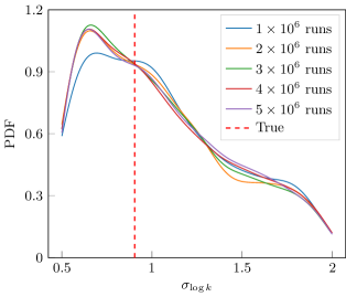
(b) $\sigma_{\log k}$

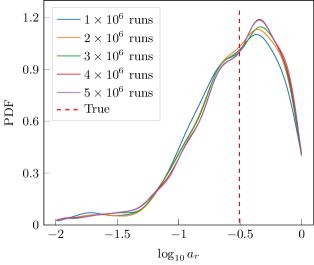
(c) $\log_{10}a_{r}$

Figure 8: Marginal posterior distributions of hyperparameters obtained using RS for true model 1. Solid curves represent the posterior distributions obtained using different numbers of forward runs. Dashed vertical lines denote the true values of the hyperparameters.

We next assess the performance of the SMC-ABC method for this problem. For an appropriate comparison to the reference RS results, we set the number of accepted samples (population size) in the SMC-ABC iterations to be consistent with the number of samples accepted in the converged RS procedure. For true model 1, the population size in SMC-ABC is set to 2500, which is close to the number of accepted samples (2584) in the reference RS results. This treatment ensures that the SMC-ABC and reference RS results have the same level of Monte Carlo approximation to the true posterior distributions.

The accuracy of the estimated posterior distributions of hyperparameters is quantified in terms of the Jensen–Shannon (JS) divergence. JS divergence is a statistical distance metric that measures the difference between two distributions, which in our case are the reference RS and approximate SMC-ABC results. JS divergence is defined as

$$\mathrm{JS}(P\|Q)=\frac{1}{2}\mathrm{KL}(P\|M)+\frac{1}{2}\mathrm{KL}(Q\|M),$$ (17)

where $P$ represents the approximate marginal posterior distribution of hyperparameters, $Q$ denotes the ‘exact’ marginal posterior distribution (taken to be the RS result with $4\times 10^{6}$ runs), and $M=\frac{1}{2}(P+Q)$ is a mixture distribution of $P$ and $Q$. The Kullback–Leibler (KL) divergence in Eq. 17 is given by

$$\mathrm{KL}(P\|M)=\int P(h)\log\Bigl{(}\frac{P(h)}{M(h)}\Bigr{)}\,\mathrm{d}h.$$ (18)

Thus we see that the JS divergence is a symmetrized and smoothed version of the KL divergence.

Results demonstrating the performance of the SMC-ABC method, with different numbers of forward runs, are presented in Fig. 9. With the number of SMC-ABC iterations increasing, the distance threshold in each iteration becomes smaller, which leads to more function evaluations. We also show the behavior of RS in terms of this metric. Immediately apparent are the large differences between the RS curves (in blue) and the SMC-ABC curves (in red). RS displays large JS divergence relative to the reference, and fairly slow convergence. The opposite is observed for SMC-ABC. This difference is particularly evident in the results for $\sigma_{\log k}$ (Fig. 9b). These results show that around $0.2\times 10^{6}$ forward runs using SMC-ABC result in a near-zero JS divergence, indicating close agreement with the reference RS results. Therefore, we use the SMC-ABC results derived from $0.2\times 10^{6}$ forward runs to compare with the reference RS.

(a) $\mu_{\log k}$

(b) $\sigma_{\log k}$

(c) $\log_{10}a_{r}$

Figure 9: Comparison of the computational efficiency for hyperparameter estimation using the RS and SMC-ABC methods. A smaller JS divergence means a more accurate estimation of the posterior distribution.

We next present results for hyperparameter estimates. In Fig. 10, the marginal posterior distributions for the three hyperparameters using SMC-ABC and RS are compared. The left column displays the reference posterior results (RS with $4\times 10^{6}$ forward runs), while the middle and right columns show the posterior distributions using the SMC-ABC and RS methods, each with $0.2\times 10^{6}$ runs. In these figures, the gray regions represent the prior distribution, green histograms are the posterior distributions, and vertical dashed lines denote the true hyperparameter values. Although the SMC-ABC distributions are slightly ‘noisier’ than the reference results, they capture the key features quite well. The RS results with $0.2\times 10^{6}$ runs, by contrast, show significant differences relative to the reference results. These differences will be shown to be even more extreme for true model 2.

(a) RS ($4\times 10^{6}$ runs)

(b) SMC-ABC ($0.2\times 10^{6}$ runs)

(c) RS ($0.2\times 10^{6}$ runs)

(d) RS ($4\times 10^{6}$ runs)

(e) SMC-ABC ($0.2\times 10^{6}$ runs)

(f) RS ($0.2\times 10^{6}$ runs)

(g) RS ($4\times 10^{6}$ runs)

(h) SMC-ABC ($0.2\times 10^{6}$ runs)

(i) RS ($0.2\times 10^{6}$ runs)

Figure 10: Marginal posterior distributions of hyperparameters for true model 1. The left column shows the posterior distributions using RS with $4\times 10^{6}$ forward runs, while the middle and right columns show the posterior distributions using SMC-ABC and RS, each with $0.2\times 10^{6}$ runs. Gray regions represent the prior distribution, green histograms are the posterior distribution, and dashed red lines denote the true values.

The pairwise marginal posterior samples obtained by the two algorithms are shown in Fig. 11. In each scatter plot, the green circles represent the joint values of two hyperparameters, and the red star indicates the true values. We see again that the SMC-ABC method with $0.2\times 10^{6}$ runs provides posterior hyperparameter samples very close to those from RS with $4\times 10^{6}$ runs. The use of RS with $0.2\times 10^{6}$ runs yields sparsely distributed joint samples (due to the very low acceptance rate of RS). These scatter plots can also provide valuable insights for posterior hyperparameter values. It is clear from Fig. 11(a) and (b), for example, that realizations corresponding to small values of both $\mu_{\log k}$ and $\sigma_{\log k}$ (or large values of both hyperparameters) would not be expected to provide simulation results in agreement with observations.

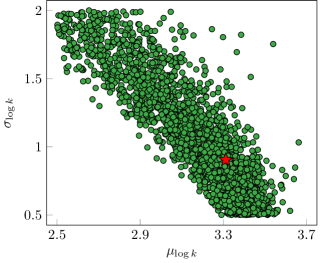
(a) RS ($4\times 10^{6}$ runs)

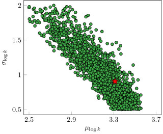
(b) SMC-ABC ($0.2\times 10^{6}$ runs)

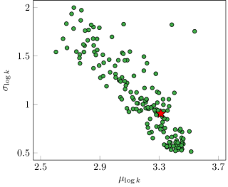
(c) RS ($0.2\times 10^{6}$ runs)

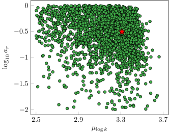
(d) RS ($4\times 10^{6}$ runs)

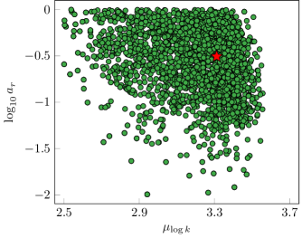
(e) SMC-ABC ($0.2\times 10^{6}$ runs)

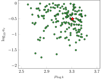
(f) RS ($0.2\times 10^{6}$ runs)

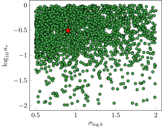
(g) RS ($4\times 10^{6}$ runs)

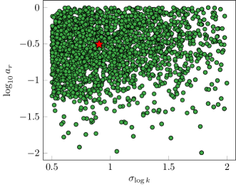
(h) SMC-ABC ($0.2\times 10^{6}$ runs)

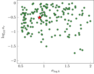
(i) RS ($0.2\times 10^{6}$ runs)

Figure 11: Pairwise marginal posterior samples of hyperparameters. Top row shows joint posterior samples of mean and standard deviation, middle row displays joint posterior samples of mean and permeability anisotropy ratio, and bottom row shows joint posterior samples of standard deviation and permeability anisotropy ratio. Green points represent posterior samples, and red stars denote true values.

The second stage of our hierarchical data assimilation approach involves the use of ESMDA to estimate the permeability field given a set of posterior hyperparameters and observed data. As noted in Section 3.3, 10 full ESMDA runs are performed, which corresponds to a total of 20,000 forward evaluations, in this second stage. The total computational cost for the hierarchical data assimilation procedure is thus $0.22\times 10^{6}$ runs. By contrast, the converged rejection sampling requires $4\times 10^{6}$ function evaluations (though reasonable results could be achieved with about half this number of runs). In either case, the hierarchical procedure provides an order of magnitude or more speedup for true model 1. As we will see, greater speedup is achieved for true model 2.

History matching results for pressure and $\mathrm{CO}_{2}$ saturation at the monitoring location are shown in Fig. 12. The gray regions represent the prior $\mathrm{P}_{10}$–$\mathrm{P}_{90}$ range, the red lines are the true data generated using the surrogate model, and the red circles are observed data. The solid blue and green curves represent the posterior $\mathrm{P}_{10}$–$\mathrm{P}_{90}$ predictions obtained from the RS procedure (with $4\times 10^{6}$ forward runs) and from the hierarchical approach, respectively. The hierarchical results are from the posterior models constructed from the 10 separate ESMDA runs. There is close agreement between the two sets of results, with substantial uncertainty reduction achieved for both pressure and saturation at the monitoring location. We see slight discrepancies between the two sets of results (e.g., $\mathrm{P}_{90}$ saturation at 5 years and $\mathrm{P}_{10}$ saturation from 10–30 years), though the differences are small.

(a) Pressure

(b) $\text{CO}_{2}$ saturation

Figure 12: History matching results for pressure (left) and $\text{CO}_{2}$ saturation (right) at the monitoring location for true model 1. Gray regions represent the prior $\mathrm{P}_{10}$–$\mathrm{P}_{90}$ range, red lines denote true data, and red circles are observed data. Solid blue and green curves denote the posterior $\mathrm{P}_{10}$ (lower) and $\mathrm{P}_{90}$ (upper) predictions obtained using the RS and hierarchical procedure, respectively.

4.3 Data assimilation results for true model 2

In the interest of brevity, we present a more limited set of results for true model 2. The posterior distributions of the hyperparameters for this case, obtained using the RS method, are shown in Fig. 13. This example is more challenging than true model 1, presumably because the true response falls at the edge of the prior. As a result, we continue to see small changes in the distributions even as we proceed from $8\times 10^{6}$ to $10\times 10^{6}$ forward runs. In fact, after $10\times 10^{6}$ runs, only 773 samples have been accepted by RS (this acceptance rate is almost an order of magnitude lower than for true model 1). Although slight shifts may still occur with larger numbers of function evaluations, we take the RS results with $10\times 10^{6}$ runs to be the reference results.

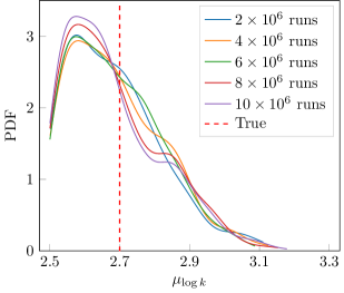
(a) $\mu_{\log k}$

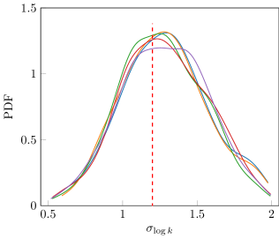
(b) $\sigma_{\log k}$

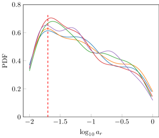
(c) $\log_{10}a_{r}$

Figure 13: Marginal posterior distributions of hyperparameters obtained from RS for true model 2. Solid curves represent the posterior distributions obtained using different numbers of forward runs. Dashed vertical lines denote the true values of the hyperparameters. Legend in (a) applies to all subplots.

The population size in SMC-ABC for true model 2 is set to 1000, which is roughly consistent with the number of accepted samples (773) from RS using $10\times 10^{6}$ runs. The behavior of the JS divergence with the number of forward runs for true model 2 (though not shown) is similar to that for true model 1. We use the SMC-ABC results derived from $0.1\times 10^{6}$ forward runs to compare with the reference RS results, as this case provides a near-zero JS divergence relative to RS with $10\times 10^{6}$ runs.

The marginal posterior distributions of hyperparameters using RS and SMC-ABC are presented in Fig. 14. A large uncertainty reduction is observed for $\mu_{\log k}$, and some reduction is achieved for $\sigma_{\log k}$. It is evident that the SMC-ABC method, with $0.1\times 10^{6}$ runs, can produce similar marginal posterior distributions for the hyperparameters as RS with $10\times 10^{6}$ runs. RS with $0.4\times 10^{6}$ runs, by contrast, results in poorly resolved approximations, as only 43 samples are accepted in this case.

History matching results for pressure and saturation at the monitoring location are shown in Fig. 15. We again observe significant uncertainty reduction and reasonable agreement in the $\mathrm{P}_{10}$ and $\mathrm{P}_{90}$ posterior predictions. Note that the $\mathrm{P}_{10}$–$\mathrm{P}_{90}$ posterior range is slightly larger with the hierarchical procedure than with RS. This was also observed in Fig. 12. Further runs would be required to determine if results shift, with either approach, with more function evaluations. In any event, our results demonstrate that the hierarchical data assimilation approach is able to generate posterior distributions and predictions that are in close correspondence with the much more expensive RS method.

(a) RS ($10\times 10^{6}$ runs)

(b) SMC-ABC ($0.1\times 10^{6}$ runs)

(c) RS ($0.4\times 10^{6}$ runs)

(d) RS ($10\times 10^{6}$ runs)

(e) SMC-ABC ($0.1\times 10^{6}$ runs)

(f) RS ($0.4\times 10^{6}$ runs)

(g) RS ($10\times 10^{6}$ runs)

(h) SMC-ABC ($0.1\times 10^{6}$ runs)

(i) RS ($0.4\times 10^{6}$ runs)

Figure 14: Marginal posterior distributions of hyperparameters for true model 2. The left column shows the posterior distributions using RS with $10\times 10^{6}$ forward runs, the middle column displays the posterior distributions using SMC-ABC with $0.1\times 10^{6}$ runs, and the right column presents the posterior distributions using RS with $0.4\times 10^{6}$ runs. Gray regions represent the prior distribution, green histograms are the posterior distribution, and dashed red lines denote the true values.

(a) Pressure

(b) $\text{CO}_{2}$ saturation

Figure 15: History matching results for pressure (left) and $\text{CO}_{2}$ saturation (right) at the monitoring location for true model 2. Gray regions represent the prior $\mathrm{P}_{10}$–$\mathrm{P}_{90}$ range, red lines denote true data, and red circles are observed data. Solid blue and green curves denote the posterior $\mathrm{P}_{10}$ (lower) and $\mathrm{P}_{90}$ (upper) predictions obtained using RS and the hierarchical procedure, respectively.

Computational requirements for both true models, in terms of forward runs, are summarized in Table 3. The hierarchical data assimilation method achieves a speedup of $83\times$ for true model 2, which is significantly larger than that for true model 1. This increased speedup is due to both an increase in the number of runs required by RS and a decrease in the number of runs for SMC-ABC (due to the smaller population size). RS is, in general, inefficient because it uses ‘brute-force’ prior sampling in the hyperparameter space to match the observed data in the data space. In the case of true model 2, because the observed pressure data fall beyond the $\mathrm{P}_{90}$ of the prior distribution, RS is particularly inefficient (i.e., even less efficient than for true model 1). The SMC-ABC approach, by contrast, focuses its computational effort on hyperparameter values that are likely to produce close matches to the observed data, which leads to substantial efficiency gains.

Table 3: Computational cost in terms of forward runs (each run entails a geostatistical simulation and a surrogate function evaluation) using RS and SMC-ABC-ESMDA, for both true models.

	RS	SMC-ABC-ESMDA	Speedup
True model 1	$4\times 10^{6}$	$0.22\times 10^{6}$	$18\times$
True model 2	$10\times 10^{6}$	$0.12\times 10^{6}$	$83\times$

5 Concluding Remarks

In this study, we developed and applied a hierarchical data assimilation framework for geological carbon storage problems. The framework uses the SMC-ABC method to estimate geomodel hyperparameters, followed by ESMDA to provide posterior realizations of grid-block permeability. An existing 3D recurrent R-U-Net deep-learning-based surrogate model was applied for function evaluations. This is an essential component of the workflow, as the overall methodology would be computationally prohibitive if high-fidelity flow simulations were used. The accuracy of the surrogate model for our case, which involved the injection of 1 Mt/year of CO₂ (for 30 years) through a single injector in the center of a 3D model, was demonstrated through comparisons to high-fidelity simulation results.

Detailed data assimilation predictions, including quantitative comparisons to a reference rejection sampling procedure, were presented for two synthetic true models. The marginal posterior distributions of the hyperparameters, pairwise marginal posterior samples, and history matching results for pressure and saturation time-series at the monitoring location were compared. Close agreement in the posterior results from the two approaches was demonstrated for both true models. This is significant, since the converged RS computations required $4\times 10^{6}$ (true model 1) and $10\times 10^{6}$ (true model 2) forward runs. Our hierarchical procedure, by contrast, needed $0.22\times 10^{6}$ and $0.12\times 10^{6}$ runs for the two cases, respectively, corresponding to speedups of $18\times$ and $83\times$ compared to RS. Thus our findings clearly demonstrate that the SMC-ABC-ESMDA procedure is able to generate accurate posterior results, with reasonable computational efficiency, for the cases considered.

There are many promising directions for future research in this area. From an algorithmic perspective, it will be of interest to improve the sampling efficiency using an active learning strategy. The integration of Bayesian optimization with likelihood-free inference has the potential to reduce the number of forward simulations, and this should be explored. For hyperparameter estimation, normalizing flows, which seek an invertible mapping between a simple base distribution and the target posterior distribution, could be considered. In terms of applications, the hierarchical framework should be extended as required to treat realistic problems. Of particular interest are cases involving sequential decision making. This is important for geological carbon storage because, in practical settings, new injection wells will be drilled and new monitoring wells will be required as the operation proceeds. SMC-based algorithms are effective for sequential decisions, and the methodology developed in this paper should be extended for this case.

CRediT authorship contribution statement

Wenchao Teng: Conceptualization, Methodology, Software, Formal analysis, Visualization, Writing – Original Draft. Louis J. Durlofsky: Conceptualization, Writing – Review and Editing, Supervision.

Declaration of competing interest

The authors declare that they have no known competing financial interests or personal relationships that could have appeared to influence the work reported in this paper.

Data availability

Please contact Wenchao Teng (wenchaot@stanford.edu) for the data or code used in this study.

References

- Akeret et al. [2015] Akeret, J., Refregier, A., Amara, A., Seehars, S., Hasner, C., 2015. Approximate Bayesian computation for forward modeling in cosmology. Journal of Cosmology and Astroparticle Physics 2015, 043–043.
- Arulampalam et al. [2002] Arulampalam, M.S., Maskell, S., Gordon, N., Clapp, T., 2002. A tutorial on particle filters for online nonlinear/non-Gaussian Bayesian tracking. IEEE Transactions on Signal Processing 50, 174–188.
- Beaumont [2010] Beaumont, M.A., 2010. Approximate Bayesian computation in evolution and ecology. Annual Review of Ecology, Evolution, and Systematics 41, 379–406.
- Beaumont et al. [2009] Beaumont, M.A., Cornuet, J.M., Marin, J.M., Robert, C.P., 2009. Adaptive approximate Bayesian computation. Biometrika 96, 983–990.
- Beaumont et al. [2002] Beaumont, M.A., Zhang, W., Balding, D.J., 2002. Approximate Bayesian computation in population genetics. Genetics 162, 2025–2035.
- Cameron and Durlofsky [2012] Cameron, D.A., Durlofsky, L.J., 2012. Optimization of well placement, CO2 injection rates, and brine cycling for geological carbon sequestration. International Journal of Greenhouse Gas Control 10, 100–112.
- Chada et al. [2018] Chada, N.K., Iglesias, M.A., Roininen, L., Stuart, A.M., 2018. Parameterizations for ensemble Kalman inversion. Inverse Problems 34, 055009.
- Chen et al. [2020] Chen, B., Harp, D.R., Lu, Z., Pawar, R.J., 2020. Reducing uncertainty in geologic CO2 sequestration risk assessment by assimilating monitoring data. International Journal of Greenhouse Gas Control 94, 102926.
- Cui et al. [2018] Cui, T., Peeters, L., Pagendam, D., Pickett, T., Jin, H., Crosbie, R.S., Raiber, M., Rassam, D.W., Gilfedder, M., 2018. Emulator-enabled approximate Bayesian computation (ABC) and uncertainty analysis for computationally expensive groundwater models. Journal of Hydrology 564, 191–207.
- Deutsch and Journel [1998] Deutsch, C.V., Journel, A.G., 1998. Geostatistical software library and user’s guide. Oxford University Press, New York.
- Emerick and Reynolds [2013] Emerick, A.A., Reynolds, A.C., 2013. Ensemble smoother with multiple data assimilation. Computers & Geosciences 55, 3–15.
- Evensen [2003] Evensen, G., 2003. The Ensemble Kalman Filter: Theoretical formulation and practical implementation. Ocean Dynamics 53, 343–367.
- Friedli et al. [2023] Friedli, L., Linde, N., Ginsbourger, D., Visentini, A.F., Doucet, A., 2023. Inference of geostatistical hyperparameters with the correlated pseudo-marginal method. Advances in Water Resources 173, 104402.
- Gelman et al. [1995] Gelman, A., Carlin, J.B., Stern, H.S., Rubin, D.B., 1995. Bayesian data analysis. Chapman and Hall/CRC.
- González-Nicolás et al. [2015] González-Nicolás, A., Baù, D., Alzraiee, A., 2015. Detection of potential leakage pathways from geological carbon storage by fluid pressure data assimilation. Advances in Water Resources 86, 366–384.
- Han et al. [2024] Han, Y., Hamon, F.P., Jiang, S., Durlofsky, L.J., 2024. Surrogate model for geological CO2 storage and its use in hierarchical MCMC history matching. Advances in Water Resources 187, 104678.
- Hansen et al. [2012] Hansen, T.M., Cordua, K.S., Mosegaard, K., 2012. Inverse problems with non-trivial priors: Efficient solution through sequential Gibbs sampling. Computational Geosciences 16, 593–611.
- Jahandideh et al. [2021] Jahandideh, A., Hakim-Elahi, S., Jafarpour, B., 2021. Inference of rock flow and mechanical properties from injection-induced microseismic events during geologic CO2 storage. International Journal of Greenhouse Gas Control 105, 103206.
- Jiang and Durlofsky [2024] Jiang, S., Durlofsky, L.J., 2024. History matching for geological carbon storage using data-space inversion with spatio-temporal data parameterization. International Journal of Greenhouse Gas Control 134, 104124.
- Kitagawa [1996] Kitagawa, G., 1996. Monte Carlo filter and smoother for non-Gaussian nonlinear state space models. Journal of Computational and Graphical Statistics 5, 1–25.
- Kitanidis [1995] Kitanidis, P.K., 1995. Quasi-linear geostatistical theory for inversing. Water Resources Research 31, 2411–2419.
- Liu and Grana [2020] Liu, M., Grana, D., 2020. Petrophysical characterization of deep saline aquifers for CO2 storage using ensemble smoother and deep convolutional autoencoder. Advances in Water Resources 142, 103634.
- Marjoram et al. [2003] Marjoram, P., Molitor, J., Plagnol, V., Tavaré, S., 2003. Markov chain Monte Carlo without likelihoods. Proceedings of the National Academy of Sciences 100, 15324–15328.
- Oliver [2022] Oliver, D.S., 2022. Hybrid iterative ensemble smoother for history matching of hierarchical models. Mathematical Geosciences 54, 1289–1313.
- Oliver and Alfonzo [2018] Oliver, D.S., Alfonzo, M., 2018. Calibration of imperfect models to biased observations. Computational Geosciences 22, 145–161.
- Papamakarios et al. [2019] Papamakarios, G., Sterratt, D., Murray, I., 2019. Sequential neural likelihood: Fast likelihood-free inference with autoregressive flows, in: Proceedings of the Twenty-Second International Conference on Artificial Intelligence and Statistics, PMLR. pp. 837–848.
- Papaspiliopoulos et al. [2007] Papaspiliopoulos, O., Roberts, G.O., Sköld, M., 2007. A general framework for the parametrization of hierarchical models. Statistical Science 22, 59 – 73.
- Prangle [2017] Prangle, D., 2017. Adapting the ABC distance function. Bayesian Analysis 12, 289 – 309.
- Reuschen et al. [2020] Reuschen, S., Xu, T., Nowak, W., 2020. Bayesian inversion of hierarchical geostatistical models using a parallel-tempering sequential Gibbs MCMC. Advances in Water Resources 141, 103614.
- Ripley [2009] Ripley, B.D., 2009. Stochastic simulation. John Wiley & Sons.
- Schlumberger [2014] Schlumberger, G., 2014. Eclipse reference manual. Schlumberger, Houston, TX.
- Seabra et al. [2024] Seabra, G.S., Mücke, N.T., Silva, V.L.S., Voskov, D., Vossepoel, F.C., 2024. AI enhanced data assimilation and uncertainty quantification applied to geological carbon storage. International Journal of Greenhouse Gas Control 136, 104190.
- Shirangi and Durlofsky [2016] Shirangi, M.G., Durlofsky, L.J., 2016. A general method to select representative models for decision making and optimization under uncertainty. Computers & Geosciences 96, 109–123.
- Sisson et al. [2018] Sisson, S.A., Fan, Y., Beaumont, M., 2018. Handbook of approximate Bayesian computation. CRC Press.
- Sisson et al. [2007] Sisson, S.A., Fan, Y., Tanaka, M.M., 2007. Sequential Monte Carlo without likelihoods. Proceedings of the National Academy of Sciences 104, 1760–1765.
- Sun and Durlofsky [2019] Sun, W., Durlofsky, L.J., 2019. Data-space approaches for uncertainty quantification of CO2 plume location in geological carbon storage. Advances in Water Resources 123, 234–255.
- Tang et al. [2022a] Tang, H., Fu, P., Jo, H., Jiang, S., Sherman, C.S., Hamon, F., Azzolina, N.A., Morris, J.P., 2022a. Deep learning-accelerated 3D carbon storage reservoir pressure forecasting based on data assimilation using surface displacement from InSAR. International Journal of Greenhouse Gas Control 120, 103765.
- Tang et al. [2021a] Tang, H., Fu, P., Sherman, C.S., Zhang, J., Ju, X., Hamon, F., Azzolina, N.A., Burton-Kelly, M., Morris, J.P., 2021a. A deep learning-accelerated data assimilation and forecasting workflow for commercial-scale geologic carbon storage. International Journal of Greenhouse Gas Control 112, 103488.
- Tang et al. [2022b] Tang, M., Ju, X., Durlofsky, L.J., 2022b. Deep-learning-based coupled flow-geomechanics surrogate model for CO2 sequestration. International Journal of Greenhouse Gas Control 118, 103692.
- Tang et al. [2021b] Tang, M., Liu, Y., Durlofsky, L.J., 2021b. Deep-learning-based surrogate flow modeling and geological parameterization for data assimilation in 3D subsurface flow. Computer Methods in Applied Mechanics and Engineering 376, 113636.
- Toni et al. [2009] Toni, T., Welch, D., Strelkowa, N., Ipsen, A., Stumpf, M.P., 2009. Approximate Bayesian computation scheme for parameter inference and model selection in dynamical systems. Journal of the Royal Society Interface 6, 187–202.
- Tran et al. [2017] Tran, D., Ranganath, R., Blei, D., 2017. Hierarchical implicit models and likelihood-free variational inference, in: Advances in Neural Information Processing Systems, Curran Associates, Inc.
- Vrugt and Sadegh [2013] Vrugt, J.A., Sadegh, M., 2013. Toward diagnostic model calibration and evaluation: Approximate Bayesian computation. Water Resources Research 49, 4335–4345.
- Wang et al. [2022] Wang, L., Kitanidis, P.K., Caers, J., 2022. Hierarchical Bayesian inversion of global variables and large-scale spatial fields. Water Resources Research 58, e2021WR031610.
- Wen et al. [2022] Wen, G., Li, Z., Azizzadenesheli, K., Anandkumar, A., Benson, S.M., 2022. U-FNO—An enhanced Fourier neural operator-based deep-learning model for multiphase flow. Advances in Water Resources 163, 104180.
- Xiao et al. [2021] Xiao, S., Xu, T., Reuschen, S., Nowak, W., Hendricks Franssen, H.J., 2021. Bayesian inversion of multi-Gaussian log-conductivity fields with uncertain hyperparameters: An extension of preconditioned Crank-Nicolson Markov chain Monte Carlo with parallel tempering. Water Resources Research 57, e2021WR030313.
- Zhao and Luo [2021] Zhao, Y., Luo, J., 2021. Bayesian inverse modeling of large-scale spatial fields on iteratively corrected principal components. Advances in Water Resources 151, 103913.