Self-Energy Approximation for the Running Coupling Constant in Thermal Theory using Imaginary Time Formalism
Abstract
The running coupling constant is calculated using the imaginary time formalism (ITF) of thermal field theory under the self-energy approximation. In the process, each Feynman diagram in thermal field theory is rewritten as the summation of non-thermal diagrams with coefficients that are functions of mass and temperature. By employing the same mass scale and coupling constant for both the non-thermal QFT and ITF, we derive a relation between them. Also, we calculate the self-energy using ITF, which is equated to the same as that of non-thermal QFT under the zero external momentum limit. This can provide a new expression for the coupling constant. Combining this result with the and function relations of the renormalization group equations gives rise to a thermal-dependent coupling constant and running mass. Using these results, the free energy density is evaluated for two-loop order and compared with quasiparticle model.
1 Introduction
The running coupling constants in various field theories play a pivotal role in describing the strength of interactions and developing equations of state Arjun2022 ; Kapusta2006 ; Khanna2009 ; Millington2014 ; Sarkar2010 ; Padmanabhan2016 . The application of such coupling constants in various phenomenological models has produced results that align with lattice data describing the interactions of particles under extreme conditions, resembling some aspects of the primordial universe Yagi2005a ; Bannur2007 ; Bannur2007a ; Bannur2007b .
In 1949, Dyson established the systematic approach to multiplicative renormalization, a method through which infinities are eliminated within the context of QED Dyson1949 . Further, concepts such as the renormalization group equation were introduced by Stueckelberg and Petermann Stueckelberg1953 , and Gell-Mann and Low GellMann1954 . A rigorous mathematical procedure for higher-order calculations using the method of counterterms, which involves a structured process for subtracting divergences, were formulated by Bogoliubow and Parasiuk Bogoliubow1957 and Hepp Hepp1966 . Later, the minimal subtraction scheme (MS Scheme) Hooft1973 ; Hooft1972 ; Weinberg1973 was developed. This scheme is an important renormalization technique in field theory, wherein Feynman integrals are computed using dimensional regularization. This approach offers several advantages, including its simplicity in identifying diverging terms and its ability to regularize nonabelian field theories while preserving gauge symmetries, among others Hooft1973 ; Hooft1972 ; Bollini1972 . Callan Callan1970 and Symanzik Symanzik1970 introduced a differential equation to study the behavior of the vertex functions under various scale approximations in the context of cutoff regularization. Subsequently, the formalism was extended to encompass the MS Scheme as well Kleinert2001 ; Padmanabhan2016 .
In the 1950s, Matsubara Matsubara1955 developed a systematic approach to describe and evaluate ensemble expectation values using quantum field theory at finite temperature, which later became popularly known as the imaginary time formalism. This method employs Wick rotation and treats the time component as an imaginary value. While there are some differences between the imaginary time formalism and zero-temperature quantum field theory, one could see a one-to-one correspondence between them, especially in the cases of Green’s functions and diagrammatic representations Kapusta1979 ; Khanna2009 ; Millington2014 .
However, the requirement of a theory for nonequilibrium systems has led to the foundation of real-time formalism at finite temperature Keldysh1964 ; Schwinger1961 ; Mahanthappa1962 ; Bakshi1963 using the closed-time path formulation. One of the important features of real-time formalism (RTF) is the doubling of the degrees of freedom. Therefore, the Green functions are expressed in matrices. Some interesting works in RTF can be found in CaronHuot2009 ; Santos2020 ; Lundberg2021 ; Carrington1999 ; Bergerhoff1998 ; Aurenche1992 ; Landsman1987 ; Ezawa1991 ; Bellac2000 ; Khanna2009 ; Millington2014 . The investigation of the coupling constant and related parameters can be explored in both real time and imaginary time. However, in this theoretical work, we prioritize the ITF. A recent and comprehensive analysis of the imaginary time formalism can be found in Mustafa2023 , which details its theoretical foundations and applications
References Kapusta2006 ; Matsumoto1984 ; Fujimoto1986 ; Fujimoto1988 discuss Renormalization Group Equations (RGE) within the framework of finite temperature field theory, in which Matsumoto1984 ; Fujimoto1986 ; Fujimoto1988 introduce multiple sets of RGE equations to calculate temperature-dependent coupling constant and mass. This is achieved by adding an additional parameter to the Lagrangian, alongside the mass scale, which results in the development of a new set of renormalization group equations. The application of both sets of RGEs to the vertex function establishes new relations among various parameters. In reference Fujimoto1986 , following the imposition of specific renormalization conditions, the authors analyzed the coupling constant and effective mass. They noted that as the temperature increases, the coupling constant decreases, while the effective mass increases. These works Fujimoto1988 ; Baier1990 ; Nakkagawa1987 ; Nakkagawa1988 collectively suggest that the nature of the coupling constant heavily depends on the choice of the vertex function.
In the 1990s, Braaten and Pisarski Braaten1990 introduced a resummation scheme using the concept of hard-thermal loops. Through its application, they provided a resummation of QCD thermal perturbation theory.
From 1992 onwards, multiple studies and calculations have analyzed the pressure and free energy density for the massless theory under various approximations, as outlined in references Frenkel1992 ; Arnold1994 ; Parwani1995a ; Andersen2009 . Similarly, Andersen et al. Andersen2000 calculated the free energy for the massive theory up to three-loop order. In recent years, modern thermal perturbation theory, particularly the hard thermal loop (HTL) approximation, has garnered new interest for calculating key thermodynamic quantities such as pressure and free energy density in high-temperature quantum field theories. This framework plays a crucial role in understanding plasmas within quantum electrodynamics (QED) and quantum chromodynamics (QCD). A thorough discussion on HTL can be found in Haque2025 . Some recent interesting studies in both thermal and non-thermal field theory can be found in references Arjun2022 ; Romatschke2023 ; Romatschke2024a ; Romatschke2024b ; Bandyopadhyay2016 ; Bandyopadhyay2016a .
Several works utilize the self-energy as an effective mass, particularly in the case of massless Lagrangian approximations under different conditions Parwani1995a ; Peshier1998 . These approximations have led to the emergence of new relations between mass and coupling constants, enabling the evaluation of diverse thermodynamic quantities and providing novel insights in the field.
In this study, we explore the non-linear temperature dependence of the mass scale, coupling constant, and running mass. This is significant because phenomenological models often use running coupling constants to introduce quantum effects and determine the effective mass of interactions. To incorporate thermal dependence in the coupling constant, these models typically assume the scale parameter to be a linear function of temperature. However, earlier works, such as Matsumoto1984 ; Fujimoto1986 , have explored alternatives to this assumption, particularly within the framework of thermal field theories. For instance, Matsumoto1984 ; Fujimoto1986 ; Fujimoto1988 employed multiple renormalization group equations (RGEs) to calculate the temperature-dependent coupling constant, particularly in the case of theory, suggesting the possibility of a non-linear temperature dependence on the scale parameter.
We show that without relying on multiple RGEs, the established RGE, as in Eq. 2, when simultaneously applied to both thermal and non-thermal vertex functions, can reveal the relationship between the mass scale, running mass, and coupling constant as functions of temperature. While a similar approach is followed in Arjun2022 , our work differs by exploring the less-studied case where the self-energy computed in ITF and QFT becomes equal. This approximation, referred to as the self-energy approximation (SEA), provides a novel perspective on these relationships. However, it is imperative that this approximation remains consistent with the Renormalization Group Equation (RGE). In this work, we focus on the Lagrangian of the following form:
| (1) |
It is already known that the renormalization group functions (, , ) associated with the renormalization group equation for the theory are identical for both non-thermal quantum field theory and the imaginary time formalism up to two-loop order Arjun2022 ; Kapusta2006 ; Laine2016 . The renormalization group equation follows a general structure of
| (2) |
where is the running coupling constant, is the running mass, and is the mass scale.
In Eq. 2, corresponds to the -point proper vertex function (PVF) Kleinert2001 . However, in this work, we are mainly dealing with two- and four-point vertex functions. The two-point vertex function is defined as the zeroth-order Feynman diagram minus the self-energy (). i.e.,
| (3) |
The finite two-point vertex function is defined as
| (4) |
Here, is an operator that extracts the pure pole terms from the dimensionally regularized integral for each diagram. Applying in Eq. 4 ensures it is finite. The detailed diagrammatic expansion of the self-energy for various orders can be found in Section 2.
The usual procedure to find the running coupling constant and running mass is through the beta function () and gamma function () relations. However, in order to determine the temperature-dependent coupling constant, one might need one additional equation that relates the coupling constant and temperature.
To enhance the clarity of calculations using diagrammatic techniques, we will introduce some convenient notations. Throughout this work, we will utilize the subscripts QFT and ITF to denote Feynman diagrams and vertex functions expressed in non-thermal quantum field theory and finite temperature imaginary time formalism, respectively. The QFT subscript denotes the vacuum part expression (i.e., field theory in four Euclidean dimensions Kapusta2006 ).
The zeroth-order Feynman diagrams with subscripts QFT and ITF are defined as
| (5) |
and
| (6) |
The substitution of , i.e., , makes Eqs. 5 and 6 equal. The use of the subscripts QFT and ITF can be further explained using diagrams and . If we denote , , , and , then the diagrams in the ITF and QFT representations can be related as shown below.
The expression for the tadpole diagram in ITF is
| (7) |
and in QFT, it is
| (8) |
Both these diagrams can be connected as
| (9) |
where
| (10) |
Similarly, the scattering diagram is defined in ITF as
| (11) |
In QFT, the corresponding expression for the diagram is
| (12) |
Both these diagrams can be connected at as
| (13) |
with
| (14) |
The important part is that having the same structure for the renormalization coefficients and renormalization function equations as in non-thermal QFT is not enough to derive the temperature-dependent running coupling constant. To derive a thermal-dependent coupling constant, Arjun2022 took a novel approach.
This approach establishes a connection between non-thermal QFT and the ITF, assuming both share the same mass scale () and coupling constant (). Hereafter, we will refer to this approach as SMC, which stands for Same Mass Scale and Coupling.
In this work, we adopt the term two-point vertex function to denote , following the convention in Kleinert2001 . While in more recent literature, the loosely related term propagator is also frequently used, the two terms refer to similar concepts with slight differences in interpretation depending on context. For the purposes of this discussion, we will adhere to the terminology two-point vertex function for consistency.
In Arjun2022 , within the SMC approximation, each Feynman diagram in ITF was expressed as the summation of Feynman diagrams in QFT, with coefficients that depend on temperature and mass. In this approach, renormalization scale independence through the RGE is imposed on the two and four-point functions for both thermal and non-thermal contributions simultaneously. This results in the usual running of renormalized parameters as a function of the renormalization scale. However, the additional constraint from the thermal part can only be satisfied by incorporating a temperature dependence of . In doing so, Arjun2022 obtains an additional equation that involves .
The process described above can be expressed mathematically as follows: the usual RGE equation demands, following the renormalization procedure (), that in the case of the finite, two-point, two-loop vertex function (),
| (15) |
and
| (16) |
for ITF and QFT, respectively Kapusta2006 ; Kleinert2001 . Since the renormalized vertex function () can be expressed as a combination of diagrams, the SMC approach, along with some Feynman diagram manipulations, allows us to connect the ITF and QFT vertex functions under the zero external momentum limit Arjun2022 as
| (17) |
It should be noted that has explicit dependence on temperature , mass , coupling constant , and mass scale . In contrast, has explicit dependence only on , , and . This does not rule out the possibility that can have temperature dependence non-explicitly via a temperature-dependent mass scale and other parameters.
When the RGE equation is applied at the two-loop order for the two-point function and combined with Eqs. 15, 16 and 17, it results in the obvious relation that,
| (18) |
This expression indicates that the mass scale needs to be temperature-dependent in such a way that it satisfies Eq. 18, along with the running mass and coupling constant.
A detailed explanation can be found in Arjun2022 and in Section 2.
Eq. 18 can be analyzed in two ways:
-
1.
, extensively examined and discussed in Arjun2022 , and
-
2.
, investigated within this study.
The former case 1) has resulted in a new relation involving the coupling constant , running mass , temperature , and mass scale . Combining this with the renormalization group function () equations has revealed how the coupling constant, running mass, and mass scale vary with temperature. Later, leveraging these relations and combining them with a quasiparticle model has demonstrated that the pressure reaches the Stefan-Boltzmann limit at high temperatures Arjun2022 .
In this work, we are exploring another possibility that has been less explored, i.e., the latter case where
| (19) |
, which is consistent with the RGE associated Eqs. 15, 16, 17 and 18. However, the relation connecting the vertex function and self-energy is , where represents self-energy and . Therefore, in the zero external momentum limit, using the relation between the two-point vertex function and the self-energy, it is possible to write Eq. 17 as follows
| (20) |
This, in turn, from Eq. 20, indicates that when , the self-energy in ITF and QFT becomes equal (see Section 2 for detailed derivation). From now onwards, we refer to this approximation as the Self-Energy Approximation (SEA). To simplify calculations, we perform them at the limit of zero external momentum. In SEA, the self-energy has a non-explicit dependence on temperature, such that the values of and other parameters are constrained in a way that always. When Eq. 19 is combined with the and relations and solved simultaneously, it results in a temperature-dependent running coupling constant , running mass , and mass scale .
Throughout this paper, we utilized the Euclidean momentum representation with to express . Some of the Feynman diagram integral results and formulas derived and utilized in this work may be found in other publications Arjun2022 ; Kapusta2006 ; Bugrij1995 ; Andersen2000 ; Andersen2001a ; Kleinert2001 . The mathematical conventions utilized in this work are established from references Arjun2022 ; Kleinert2001 .
This work is organized as follows: In Section 2, we establish a connection by writing down all essential diagrams and counter diagrams in the finite temperature imaginary time formalism (ITF) in terms of the corresponding diagrams in quantum field theory (QFT). In Section 3, a new relation for the coupling constant, mass scale, running mass, and temperature is derived using renormalization group function relations and self-energy approximation (SEA). The evaluation of the running mass, coupling constant, and mass scale is then combined with the renormalization group functions.
Over the past few decades, the study of Quark-Gluon Plasma (QGP) has advanced significantly through various phenomenological models, including quasiparticle models Bannur2007 ; Bannur2007a ; Bannur2007b ; Peshier1994 ; Peshier1996 ; Peshier1998 that account for the non-ideal behavior of QGP observed in both lattice QCD simulations and heavy-ion collision experiments. These models often approximate the effective mass of the interacting particles as a function of the coupling constant, typically expressed as , where is the temperature-dependent coupling constant. While this paper primarily focuses on the thermodynamic properties of theory, it also draws upon insights from these quasiparticle models to establish a comparative framework. Specifically, we examine the free energy density of the massive theory and its relation to the quasiparticle model. In Section 4, the values of the running mass, coupling constant, and mass scale are applied to these models, and the pressure and free energy are evaluated for various orders and parameters.
2 Regularization
The diagrams in theory can be described as compositions of fundamental, non-trivial Feynman diagrams known as one-particle irreducible (1 PI) diagrams. Eqs. 21 and 23 represent the two-point vertex function at different orders, each composed of 1 PI diagrams. The composition of all 1PI diagrams, excluding the zeroth-order one, is termed the self-energy and is often represented by Kleinert2001 ; Padmanabhan2016 .
The general structure of two-point one-loop order vertex function is
| (21) |
where is the self-energy at the one loop approximation with
| (22) |
The general structure of two-point two-loop order vertex function is
| (23) |
with
| (24) |
where is the self-energy at the two-loop approximation. As one evaluates the diagrams in Eqs. 22 and 24 using dimensional regularization Kleinert2001 ; Hooft1972 ; Hooft1973 , divergences appear. These divergences can be removed by introducing appropriate counterterms defined using the minimal subtraction scheme (MS-Scheme).
The self-energy diagrams for one and two-loop approximation with counterterms can be expressed as
| (25) |
and
| (26) |
In Sections 2.1 and 2.2, we follow the dimensional regularization procedure Kleinert2001 and analyze the self-energy diagrams shown in Eqs. 25 and 26 in both ITF and QFT for one-loop and two-loop orders, respectively, using the approximation . It should be noted that in the context of finite terms, as .
2.1 One loop order two point function
The one-loop order two-point vertex function Kleinert2001 in general form can be written as
| (27) |
However, one could relate the above tadpole diagram in ITF with a similar QFT diagram using Eqs. 9, 8 and 7 at as
| (28) |
with
| (29) |
(See Section A.1 for detailed derivation).
Thus, it is evident that the divergence that comes in the ITF diagram shown in Eq. 28 at the one-loop order originates from the corresponding diagram in QFT, or in other words, the divergence parts of both of these diagrams are the same. It is clear from Eq. 8 corresponding to the QFT diagram that the integral is diverging. On substituting and , we can isolate the term which diverges at the limit Kleinert2001 .
Therefore, the analytical expression can be written up to the first order as
| (30) |
where
| (31) |
| (32) |
with
| (33) |
is Euler’s constant.
To make the two-point vertex function finite, counterterms can be defined to cancel the divergences Kleinert2001 .
and are called mass counterterm and momentum counterterm respectively Kleinert2001 .
The counterterms can be determined using the pole-picking operator, denoted as , where for .
Therefore
| (34) |
i.e., at the one loop order . For the sake of completeness, it is important to note that the momentum counter term at one-loop order is zero.
| (35) |
The general finite vertex function at one-loop order is thus
| (36) |
The specific versions for ITF and QFT can be written as
| (37) |
| (38) |
At the zero external momentum limit, or at , the two-point one-loop order finite vertex function in ITF and QFT can be connected using Eqs. 34, 36, 28, 37 and 38 as
| (39) |
.
2.2 Two-loop order two point functions
At the two-loop approximation, the first-order counter term defined earlier to make the one-loop finite vertex function can produce some extra diagrams (referred to as counterterm diagrams) in addition to the second-order diagrams. i.e.,
| (40) |
We use the following notations:
| (41) |
The diagrams in Eqs. 24 and 40, aside from the tadpole diagram already explained in Eqs. 9, 8 and 7, can be expressed mathematically in ITF and QFT as follows:
| (42) |
| (43) |
At the limit , and , the diagrams in ITF and QFT can be connected as
| (44) | ||||
where
| (45) |
A detailed derivation of Eq. 44 with necessary steps can be found in Section A.2.
The expression for in ITF and QFT are
| (46) |
and
| (47) |
respectively. At the limit of zero external momentum (=0), the diagram in ITF and QFT can be linked () as
| (48) | ||||
where
| (49) |
with
| (50) |
| (51) |
(Refer to Section A.4 for a detailed derivation).
The counterterm diagrams can also be connected in a similar manner.
| (52) |
The comprehensive derivation of the counterterm illustrated in Eq. 52, including all essential steps, is presented in Section B.2.
The remaining counterterm diagram’s ITF and QFT relation from Section B.3 is
| (53) |
By combining the relations from Eqs. 28, 44, 52, 48 and 53 and applying them to Eq. 40, at the limit as , it becomes clear that the divergence of the non-finite two-point vertex function at the two-loop order for ITF is identical to that of QFT.
| (54) |
Combining this with Eq. 23 also implies
| (55) |
The vertex function can be made finite by subtracting the poles term, which can be determined by applying the operator, i.e.,
| (56) | ||||
In order to simplify further calculations, let us define a new operator such that
| (57) |
where represents the appropriate diagram.
Using this new notation, the finite vertex functions can be correlated under SMC as shown below.
| (58) |
where
| (59) |
with
| (60) |
| (61) | ||||
| (62) | ||||
In reference Arjun2022 , it was demonstrated that the divergence factors of two-point and four-point vertex functions for both ITF and QFT were in the same form. Likewise, the renormalization group functions, such as beta () and gamma (), exhibited similar formats for both ITF and QFT approximations. Subsequently, in Arjun2022 , the renormalization group equation was simultaneously applied to both vertex functions in ITF and QFT. The resulting expression established a new coupling constant relation. In other words, when the RGE equations were applied and approximated as
| (63) |
and
| (64) |
, they resulted in
| (65) |
. Upon solving this with the assumption , we obtained a new coupling constant relation in addition to the beta and gamma function relations. These relations were simultaneously solved in reference Arjun2022 under the same mass scale and coupling approximation, and the running mass and running coupling constant were computed numerically.
3 Self-energy Approximation
The other possibility, apart from Arjun2022 , where becomes zero is when itself is zero. By setting to zero and combining Eqs. 58 and 23, we find that
| (66) |
That is, when the self-energy function of both ITF and QFT becomes equal. Therefore
| (67) |
Combining LABEL:gammadiffzero with Eqs. 59, 60, 61 and 62 we get the non-trivial expression
| (68) |
where
| (69) | ||||
and the expressions for , and are given in Eqs. 32, 49 and 45, respectively.
If we combine with beta coupling constant relation Kleinert2001 such as
| (70) |
give rise to the result
| (71) |
Similarly, the corresponding running mass coupling relation is
| (72) |
When combined with Eq. 70, it results in
| (73) | ||||
| i.e., |
where , and are the respective integration constants. To simplify the equation further, we choose the integration constants . In the zero momentum limit, we choose , , and Arjun2022 ; Kleinert2001 .
Solving Eqs. 71, 73 and 68 simultaneously, we obtain the temperature-dependent running mass, mass scale and coupling constant.
3.1 Free energy contribution from temperature dependent terms in the vacuum diagrams
Following the conventions in reference Kleinert2001 , the zero-point vertex function can be written as
| (74) |
and the free energy density Laine2016 as
| (75) |
where
| (76) |
| (77) |
The expression in Eq. 75 represents the non-finite version of free energy density. The one-loop vacuum diagram stands alone as the only diagram devoid of any vertex. Following some algebraic manipulations, the thermal and non-thermal diagrams can be connected at the one-loop order as
| (78) |
with
| (79) |
See Section C.1 for detailed derivation. As we expand it in the powers of Kleinert2001 we have
| (80) |
Similarly
| (81) |
The braces serve as labels rather than multiplication factors. As
| (82) |
Refer to Section C.2 for a comprehensive derivation. From Kleinert2001 , we have
| (83) | ||||
However, if we include the vacuum counter term following the same procedures as in Kapusta1979 ; Kapusta2006 and in Section C.3, then the counter terms in thermal and non-thermal QFT can be expressed as
| (84) |
where
| (85) |
These results also indicate that the two-loop order zero-point vertex function in ITF and non-thermal QFT are having the same order of divergence if counterterms are considered. i.e., the divergence/pole terms of one-loop vacuum diagram for non-thermal QFT and ITF are the same under SMC ( See Eq. 78 ).
| (86) |
The same trend can be seen in the summation of two-loop vacuum diagrams (Eq. 81) with the counterterm (Eq. 84) as shown below
| (87) |
Therefore, at , using Eqs. 78, 82 and 57, we get
| (88) | ||||
| (89) |
The quantity is finite. This result corresponds to the two-loop contribution to finite free energy density, while the first term corresponds to the one-loop. This expression matches the free energy expression in Andersen2000 , albeit with a difference in the choice of coupling (using instead of ), along with some minor conventional distinctions. As we substitute the temperature-dependent running mass, running coupling, and mass scale obtained from the previous section into the expression for the finite free energy density, we can determine how the finite free energy density varies with respect to temperature. Now at limit we can write
| (90) | ||||
| (91) |
At the massless limit, is identical with the corresponding pressure expression for theory given in reference Kapusta2006 . The only distinction lies in our usage of theory, whereas in reference Kapusta2006 , theory is employed, resulting in a factor difference of in the pressure expression’s terms involving the coupling. Incorporating this multiplicative correction will reconcile both expressions.
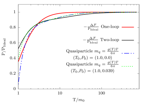
The free energy density vs. temperature relation becomes particularly interesting when we apply the temperature-dependent running coupling constant, running mass, and mass scale derived from the previous section. When applied here, it provides the temperature vs. free energy density relation, as shown in Fig. 2, which is novel. This is because the coupling constant is computed without relying on multiple RGEs, but rather by simply applying the already established RGE equations to both thermal and non-thermal vertex functions simultaneously.
3.2 Pressure evaluation using quasi-particle model
Several phenomenological models have been proposed to explain the non-ideal behavior of Quark-Gluon Plasma (QGP) observed in lattice QCD simulations and heavy-ion collision experiments. These include the strongly interacting QGP (sQGP) model Shuryak2005 , in which the presence of various neutral and colored bound states, arising from Coulomb interactions, leads to non-ideal effects. Another significant approach is the strongly coupled QGP (SCQGP) model, which draws an analogy between QGP near the critical temperature and a strongly coupled plasma (SCP) in QED, employing a modified equation of state to better align QCD lattice data Bannur2006 . Among these, the quasiparticle QGP (qQGP) model has emerged as one of the most successful frameworks, describing QGP as a medium composed of quasiparticles with temperature-dependent effective masses. Although initial formulations Goloviznin1993 ; Peshier1994 encountered thermodynamic inconsistencies, subsequent refinements—such as rederiving the model from the energy density—have resolved these issues Bannur2007a , making quasiparticle models a robust tool for investigating the thermodynamic properties of QGP. In this section, we extend this approach to the theory, comparing the resultant pressure with the free energy density.
According to the quasiparticle model in Bannur2007 ; Bannur2007a ; Bannur2007b , the quasiparticle mass per temperature is proportional to the coupling constant i.e., . The energy density and pressure of a particle obeying the Bose-Einstein distribution can be derived as
| (92) | ||||
where is the modified Bessel function of the second kind, and
.
We have energy density - pressure relation as
| (93) |
We define following the quasi-particle framework Bannur2007 ; Bannur2007a ; Bannur2007b , and select the parameters and ,. Subsequently, we obtain a quasiparticle pressure as depicted in Fig. 2. Notably, different choices of and values can be considered. These choices may be informed by lattice data, once such data becomes available.
4 Results and Discussion
In this study, we revisit reference Arjun2022 and compute the running mass, mass scale, and running coupling constant for the massive theory within the framework of the self-energy approximation. Within this approximation, we impose the condition that the self-energy calculated at the zero external momentum limit in the Imaginary Time Formalism (ITF) equals that of non-thermal Quantum Field Theory (QFT) under the same mass scale and coupling approximation (SMC). This finding is consistent with existing renormalization group equations. It has been previously demonstrated in Arjun2022 , that the Renormalization Group (RG) functions take the same form for both QFT and ITF under SMC.
By simultaneously solving the renormalization group functions and , as represented by Eqs. 73 and 71, with the self-energy approximation expression for in Eq. 68, we obtain temperature-dependent solutions for the running mass, running coupling constant, and mass scale.
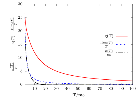
We present the main result in Figs. 1 and 2, focusing on the simple approximation of zero external momentum limit. In Fig. 1, we plot scaled functions of the two-loop coupling constant, running mass per temperature, and mass scale on the y-axis as a multi-variable plot. This approach is chosen to provide a comprehensive visualization of the relationships between various quantities as functions of temperature. From Fig. 1, it becomes apparent that there exists a negative correlation between the running mass and temperature, as well as between the running coupling and temperature. Additionally, a negative correlation is observed between the mass scale and temperature. These findings indicate that as temperature increases, the values of the running mass, running coupling, and mass scale tend to decrease, although with varying degrees of change.
Thermodynamic quantities such as pressure and free energies are closely related Kapusta2006 . It is well-known that at high temperature limits, the system pressure should approach the ideal Stefan-Boltzmann limit. This provides a useful tool for validating the running mass, coupling constant, and mass scale. Various approaches and models exist for determining thermodynamic quantities. One famous model is the quasiparticle model, where the energy density is calculated by integrating the relativistic energy function over the Bose-Einstein distribution Bannur2007 ; Bannur2007a ; Bannur2007b . Integrating the energy density per temperature squared with respect to temperature yields the pressure per temperature, as shown in Eq. 93. This pressure relation depends on the running coupling constant and temperature. Applying the running coupling constant-mass relation () to the equation Eq. 92 yields the plot shown in Fig. 2, where it is evident that the pressure reaches the ideal limit as temperature increases.
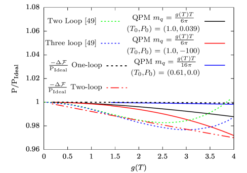
Fig. 3 compares the pressure calculated using the quasiparticle model (QPM) and the free energy density calculated using the SEA with the massless theory under the effective field theory framework Andersen2009 . At low values of the running coupling constant , both models predict similar ratios of pressure to ideal pressure. However, as increases, their distinct approaches lead to increasingly different results. This difference is understandable, as the analysis in Andersen2009 employs weak coupling to derive the pressure. The QPM depends on the initial pressure parameters and . The figure includes plots for various combinations of and to illustrate the dependence of QPM results on these parameters. Since the effective mass in the QPM is proportional to , we have also plotted results using different proportionality constants for comparison. To determine the most accurate proportionality constant and the optimal values of , lattice data will be crucial. The free energy density calculated using the SEA approach is a function of the running mass, running coupling constant, and mass scale. However, the relationship between and free energy density may not fully capture the essence of the system. In this context, a comparison of temperature () versus free energy density may be more relevant. This discussion naturally leads us to Figure 2, where we compare the free energy and pressure against temperature using a similar approach for the coupling constant.
In Fig. 2 the approach involves computing free energy relations using vacuum diagrams. In contrast to the quasiparticle model, which primarily relies on the running coupling constant, the finite free energy density at the one-loop approximation heavily depends on the running mass. However, the free energy density derived from two-loop vacuum diagrams is influenced by the running mass, coupling constant, and mass scale. Therefore, it is a preferable method for assessing the validity of all three parameters. In this work, we have expressed the finite free energy density using the same conventions that were employed to derive the coupling constant. It should be noted that the quasiparticle model, utilizing the mass approximation , at , closely aligns with the negative of the two-loop free energy density near low-temperature and very high-temperature limits. However, the absence of lattice data hinders a robust parameter fitting process. Nevertheless, the comparison underscores the quasiparticle model’s flexibility, particularly through parameters such as the proportionality constant connecting mass per temperature with the coupling constant and the integration constant parameters , distinguishing it from other models. As observed in the Fig. 2, for both one and two-loop approximations, the negative of the finite free energy density reaches the ideal Stefan-Boltzmann limit at high temperatures.
5 Conclusion
In this work, we have demonstrated that it is possible to derive the running mass and running coupling constant consistently without relying on multiple sets of renormalization group equations. A simultaneous application of the existing RGE equation to the imaginary time formalism and non-thermal quantum field theory is sufficient to derive the running mass and coupling constant. Our approach offers a more straightforward method for studying the running coupling constant, effective mass, and mass scale.
Here we employ a self-energy approximation (SEA) at zero external momentum limit, resulting in a trivial solution for the running coupling constant , running mass , and mass scale . In SEA under Same Mass Scale and Coupling approximation (SMC), the self-energy of non-thermal Quantum Field Theory (QFT) and Imaginary Time Formalism (ITF) are considered equal, aligning with the renormalization group equation. This also implies that in SEA, the finite vertex function for both ITF and non-thermal QFT becomes the same, leading to an additional relation connecting temperature with the coupling constant, mass scale, and running mass, alongside the renormalization group functions and (Eqs. 68, 70, 71, 72 and 73). Solving these relations simultaneously yields temperature-dependent running mass, mass scale, and coupling function.
The pressure and free energy density are calculated using different formulations. To calculate the pressure, we employed the quasiparticle model, where the pressure is a function of the coupling constant and temperature. The free energy density is determined by a function derived from vacuum diagrams involving the running mass, coupling constant, and mass scale. Evaluation has shown that these quantities reach their ideal limits at higher temperatures. Once lattice data or experimental data becomes available within a certain range, it would be intriguing to adjust various integration constants and compare the outcomes. Additionally, extending this model to Quantum Electrodynamics (QED) and Quantum Chromodynamics (QCD) could provide valuable insights into their behavior Arjun2024 .
References
- [1] K. Arjun, A. M. Vinodkumar, and V. M. Bannur, Running coupling constant in thermal theory up to two loop order, Phys. Rev. D 105 (Jan, 2022) 025023.
- [2] J. I. Kapusta and C. Gale, Finite-Temperature Field Theory. Cambridge University Press, 2006.
- [3] F. C. Khanna, ed., Thermal quantum field theory. World Scientific Pub. Co, Singapore, 2009. Includes bibliographical references (p. 445-455) and index.
- [4] P. Millington, Thermal Quantum Field Theory and Perturbative Non-Equilibrium Dynamics. Springer International Publishing, 2014.
- [5] S. Sarkar, H. Satz, and B. C. Sinha, eds., The Physics of the Quark-Gluon Plasma: Introductory Lectures. No. 785. Springer Berlin Heidelberg, 2010.
- [6] T. Padmanabhan, Quantum Field Theory. Springer International Publishing, 2016.
- [7] K. Yagi, T. Hatsuda, and Y. Miake, Quark-gluon plasma: From Big Bang to Little Bang. Cambridge Univ. Press, 2005.
- [8] V. M. Bannur, Revisiting the quasi-particle model of the quark–gluon plasma, Eur. Phys. J C 50 (feb, 2007) 629–634.
- [9] V. M. Bannur, Comments on quasiparticle models of quark–gluon plasma, Phys. Lett. B 647 (apr, 2007) 271–274.
- [10] V. M. Bannur, Self-consistent quasiparticle model for quark-gluon plasma, Phys. Rev. C 75 (apr, 2007) 044905.
- [11] F. J. Dyson, The matrix in quantum electrodynamics, Phys. Rev. 75 (Jun, 1949) 1736–1755.
- [12] Stueckelberg, E.C.G. and Petermann, A., La normalisation des constantes dans la théorie des quanta, Helv. phys. acta (1953).
- [13] M. Gell-Mann and F. E. Low, Quantum electrodynamics at small distances, Phys. Rev. 95 (Sept., 1954) 1300–1312.
- [14] N. N. Bogoliubow and O. S. Parasiuk, Über die multiplikation der kausalfunktionen in der quantentheorie der felder, Acta Math. 97 (1957), no. 0 227–266.
- [15] K. Hepp, Proof of the bogoliubov-parasiuk theorem on renormalization, Commun. Math. Phys. 2 (Dec., 1966) 301–326.
- [16] G. ’t Hooft, Dimensional regularization and the renormalization group, Nucl. Phys. B 61 (sep, 1973) 455–468.
- [17] G. ’t Hooft and M. Veltman, Regularization and renormalization of gauge fields, Nucl. Phys. B 44 (jul, 1972) 189–213.
- [18] S. Weinberg, New approach to the renormalization group, Phys. Rev. D 8 (Nov., 1973) 3497–3509.
- [19] C. G. Bollini and J. J. Giambiagi, Dimensional renorinalization : The number of dimensions as a regularizing parameter, Il Nuovo Cimento B (1971-1996) 12 (Nov, 1972) 20–26.
- [20] C. G. Callan, Broken scale invariance in scalar field theory, Phys. Rev. D 2 (oct, 1970) 1541–1547.
- [21] K. Symanzik, Small distance behaviour in field theory and power counting, Commun. Math. Phys. 18 (sep, 1970) 227–246.
- [22] H. Kleinert and V. Schulte-Frohlinde, Critical Properties of Phi4-Theories. World Scientific, jul, 2001.
- [23] T. Matsubara, A new approach to quantum-statistical mechanics, Prog. Theor. Phys. 14 (Oct., 1955) 351–378.
- [24] J. I. Kapusta, Infrared properties of quark gas, Phys. Rev. D 20 (aug, 1979) 989–995.
- [25] L. Keldysh Sov. Phys. JETP 47 (1965) 1515–1527.
- [26] J. Schwinger, Brownian motion of a quantum oscillator, J. Math. Phys. 2 (May, 1961) 407–432.
- [27] K. T. Mahanthappa, Multiple production of photons in quantum electrodynamics, Phys. Rev. 126 (Apr., 1962) 329–340.
- [28] P. M. Bakshi and K. T. Mahanthappa, Expectation value formalism in quantum field theory. ii, J. Math. Phys. 4 (Jan., 1963) 12–16.
- [29] S. Caron-Huot, Hard thermal loops in the real-time formalism, J. High Energy Phys. 2009 (Apr., 2009) 004–004.
- [30] A. F. dos Santos and F. C. Khanna, Bhabha scattering in very special relativity at finite temperature, Eur. Phys. J. C 80 (Aug., 2020).
- [31] T. Lundberg and R. Pasechnik, Thermal field theory in real-time formalism: concepts and applications for particle decays, Eur. Phys. J. A 57 (Feb., 2021).
- [32] M. Carrington, H. Defu, and M. Thoma, Equilibrium and non-equilibrium hard thermal loop resummation in the real time formalism, Eur. Phys. J. C 7 (Feb., 1999) 347–354.
- [33] B. Bergerhoff, Critical behavior of -theory from the thermal renormalization group, Phys. Lett. B 437 (Oct., 1998) 381–389.
- [34] P. Aurenche and T. Becherrawy, A comparison of the real-time and the imaginary-time formalisms of finite-temperature field theory for 2, 3 and 4-point green functions, Nucl. Phys. B 379 (July, 1992) 259–303.
- [35] N. Landsman and C. van Weert, Real- and imaginary-time field theory at finite temperature and density, Phys. Rep. 145 (Jan., 1987) 141–249.
- [36] H. Ezawa, Thermal Field Theories. North-Holland Delta Series. Elsevier Science, Burlington, 1991. Description based upon print version of record.
- [37] M. L. Bellac, Thermal field theory. Cambridge monographs on mathematical physics. Cambridge University Press, Cambridge, 1. paperback ed. (with corrections) ed., 2000. Includes bibliographical references. - Originally published: 1996.
- [38] M. G. Mustafa, An introduction to thermal field theory and some of its application, The European Physical Journal Special Topics 232 (July, 2023) 1369–1457.
- [39] H. Matsumoto, Y. Nakano, and H. Umezawa, Renormalization group at finite temperature, Phys. Rev. D 29 (mar, 1984) 1116–1124.
- [40] Y. Fujimoto, K. Ideura, Y. Nakano, and H. Yoneyama, The finite temperature renormalization group equation in theory, Phys. Lett. B 167 (Feb., 1986) 406–410.
- [41] Y. Fujimoto and H. Yamada, Finite-temperature renormalization group equation in QCD. II, Phys. Lett. B 200 (jan, 1988) 167–170.
- [42] R. Baier, B. Pire, and D. Schiff, High temperature behaviour of the QCD coupling constant, Phys. Lett. B 238 (apr, 1990) 367–372.
- [43] H. Nakkagawa and A. Niégawa, Temperature dependence of the non-abelian gauge couplings at finite temperature, Phys. Lett. B 193 (jul, 1987) 263–267.
- [44] H. Nakkagawa, A. Niégawa, and H. Yokota, Non-abelian gauge couplings at finite temperature in the general covariant gauge, Phys. Rev. D 38 (oct, 1988) 2566–2578.
- [45] E. Braaten and R. D. Pisarski, Resummation and gauge invariance of the gluon damping rate in hot QCD, Phys. Rev. Lett. 64 (mar, 1990) 1338–1341.
- [46] J. Frenkel, A. V. Saa, and J. C. Taylor, Pressure in thermal scalar field theory to three-loop order, Phys. Rev. D 46 (oct, 1992) 3670–3673.
- [47] P. Arnold and C. Zhai, Three-loop free energy for pure gauge QCD, Phys. Rev. D 50 (dec, 1994) 7603–7623.
- [48] R. Parwani and H. Singh, Pressure of hotg24theory at orderg5, Phys. Rev. D 51 (apr, 1995) 4518–4524.
- [49] J. O. Andersen, L. T. Kyllingstad, and L. E. Leganger, Pressure to orderg8loggof massless 4theory at weak coupling, J. High. Energy Phys. 2009 (aug, 2009) 066–066.
- [50] J. O. Andersen, E. Braaten, and M. Strickland, Massive basketball diagram for a thermal scalar field theory, Phys. Rev. D 62 (jul, 2000) 045004.
- [51] N. Haque and M. G. Mustafa, Hard thermal loop—theory and applications, Progress in Particle and Nuclear Physics 140 (Jan., 2025) 104136.
- [52] P. Romatschke, Negative coupling on the lattice, arXiv (2023).
- [53] P. Romatschke, Life at the landau pole, AppliedMath 4 (Jan., 2024) 55–69.
- [54] P. Romatschke, Alternative to perturbative renormalization in ( 3+1 )-dimensional field theories, Phys. Rev. D 109 (June, 2024) 116020.
- [55] A. Bandyopadhyay, C. A. Islam, and M. G. Mustafa, Electromagnetic spectral properties and debye screening of a strongly magnetized hot medium, Phys. Rev. D 94 (Dec., 2016) 114034.
- [56] A. Bandyopadhyay, N. Haque, M. G. Mustafa, and M. Strickland, Dilepton rate and quark number susceptibility with the gribov action, Phys. Rev. D 93 (Mar., 2016) 065004.
- [57] A. Peshier, B. Kämpfer, O. P. Pavlenko, and G. Soff, Thermodynamics of the phi4-theory in tadpole approximation, Euro. Phys Lett. 43 (aug, 1998) 381–385.
- [58] M. Laine and A. Vuorinen, Basics of Thermal Field Theory: A Tutorial on Perturbative Computations. Springer International Publishing, 2016.
- [59] A. I. Bugrij and V. N. Shadura, Three-loop contributions to the free energy of qft, arxiv (1995) [hep-th/9510232v2].
- [60] J. O. Andersen, E. Braaten, and M. Strickland, Screened perturbation theory to three loops, Phys. Rev. D 63 (apr, 2001) 105008.
- [61] A. Peshier, B. Kämpfer, O. Pavlenko, and G. Soff, An effective model of the quark-gluon plasma with thermal parton masses, Phys. Lett. B 337 (oct, 1994) 235–239.
- [62] A. Peshier, B. Kämpfer, O. P. Pavlenko, and G. Soff, Massive quasiparticle model of the SU(3) gluon plasma, Phys. Rev. D 54 (aug, 1996) 2399–2402.
- [63] E. Shuryak, What rhic experiments and theory tell us about properties of quark–gluon plasma?, Nucl. Phys. A 750 (Mar., 2005) 64–83.
- [64] V. M. Bannur, Strongly coupled quark gluon plasma (scqgp), J. Phys. G 32 (May, 2006) 993–1002.
- [65] V. Goloviznin and H. Satz, The refractive properties of the gluon plasma in SU(2) gauge theory, Zeit. für Phys. C 57 (dec, 1993) 671–675.
- [66] K. Arjun et al., A revisit to running coupling constant in qed and qcd in the context of thermal field theory, unpublished.
Appendix A Two point function evaluation
A.1 Diagram 1
An essential equation for deriving the Feynman diagram in the finite temperature imaginary time formalism (ITF) can be expressed as follows:
| (94) | ||||
where is the modified Bessel function of the second kind and , with and . Using the above relation, it is possible to express
| (95) | ||||
In the context provided, the braces serve as labels rather than multiplication factors. Upon proceeding with dimensional regularization, the Feynman diagram undergoes a substitution , resulting in
| (96) |
with
| (97) |
and
| (98) |
, where we utilize a standard result from Kleinert2001 . The validity of Eq. 96 can be confirmed through a similar integral result found in Andersen2000 ; Peshier1998 . The primary distinction lies in our definition of
| (99) |
, whereas in Andersen2000 ; Peshier1998 , it is defined as
| (100) |
A.2 Diagram 2
| (101) | ||||
At and , we can write
| (102) | ||||
From Kleinert2001 we can express
| (103) | ||||
| (104) |
and from Eq. 96 and Kleinert2001
| (105) |
A.3 Diagram 3
Utilizing Feynman diagrams corresponding to the four-point functions as outlined in Arjun2022 , we derived the renormalization constants and renormalization group function for the finite temperature imaginary time formalism (ITF). It has been demonstrated that the renormalization group function exhibits the same structure in both ITF and non-thermal quantum field theory (QFT). Although this diagram is not directly referenced in the main body of this paper, it holds significant importance in calculating the counterterm diagrams. In this context, we formulate using references Arjun2022 ; Kleinert2001
| (106) | |||
Corresponding diagrammatic expression with at is
| (107) |
with
| (108) |
Utilizing dimensional regularization and drawing from the result in the standard textbook Kleinert2001 , we can express that
| (109) | ||||
| (110) |
with
A.4 Diagram 4
The formulas provided in Section A.3 will prove beneficial as we divide the sunrise/sunset diagrams into subdiagrams. With references Arjun2022 ; Kleinert2001 ; Kapusta2006 for support, we can express the integral expression for the sunrise/sunset diagram in ITF as follows:
| (111) |
From Bugrij1995 ; Andersen2000 ; Andersen2001a , the integral can be expressed as , where
| (112) |
with , and
with and
| (113) |
However, the third term can be written as
with . Now by referring to the corresponding result from Kleinert2001 and Section A.3, we can write
| (114) |
where
| (115) |
with .
| (116) | ||||
Let us simplify by setting ,
| (117) |
Now, combining the results, we can express the terms that diverge (i.e., the pole terms) as follows:
| (118) | ||||
At the external momentum , and as , the integral result is
| (119) | ||||
with
| (120) |
and
| (121) | |||
| (122) |
The approximation can be verified using results from Andersen2001a
Appendix B Counterterms
B.1 Counterterm 1
This counterterm does not directly appear in the main text; however, it holds essential significance for the calculation of four-point functions as well as certain two-point counterterm calculations Arjun2022 . From Kleinert2001 , the counter term for divergence for the four-point function derived is
| (123) |
The corresponding diagram in imaginary time formalism Arjun2022 is
| (124) |
From Section A.3, it is evident that the diverging term is identical for the diagram in the imaginary time formalism and non-thermal QFT. Consequently, we can express
| (125) |
The same pole term can be also expressed at as
| (126) |
B.2 Counterterm 2
Following the same procedure and convention as outlined in Kleinert2001 , if we define the operator as the substitution of the counter term or , we can express the counter terms as:
| (127) | ||||
From Section A.1, we have the relation
| (128) |
Therefore, for ITF, the corresponding derivation is
| (129) | ||||
So using the results from Kleinert2001 , the above equation can be reduced as
| (130) |
B.3 Counterterm 3
From Kleinert2001 , the calculation proceeds as
| (131) | ||||
the corresponding diagram made with results from Appendices Eqs. 96 and A.3 is
| (132) | ||||
The result can also be expressed as
| (133) |
Appendix C Vacuum Diagrams
C.1 Vacuum diagram 1
The analytic expression for the one-loop diagram in non-thermal QFT in dimension Kleinert2001 is
| (134) |
and that of ITF is
| (135) |
Following the same procedures as in Kleinert2001 and doing some algebraic manipulations in Eq. 94
| (136) |
One might argue that the logarithm of the vacuum diagram displayed above lacks dimensional coherence, as its argument possesses dimensions of mass squared. Ideally, it should resemble a dimensionless form, such as , where represents a mass scale. However, within the context of dimensional regularization, this manner of expressing the logarithm does not alter the integral. A detailed discussion, supported by the Veltman formula, can be found in Kleinert2001 . Since the integral is free of the vertex (), we will have to go through some other procedures described in Kleinert2001 , like multiplying the integral by a unit factor and expanding in powers of as . Therefore
| (137) |
and
| (138) |
C.2 Vacuum diagram 2
The two-loop diagram corresponds to the Feynman integral for QFT, can be written as
| (139) |
The corresponding expression in ITF can be connected with that of QFT using Eq. 96 as
| (140) | ||||
From Kleinert2001 , the QFT diagram can be expanded in powers of at as
| (141) |
C.3 Vacuum counterterm
The vacuum counterterm can be derived using the ideas in Kapusta2006 as follows:
| (142) | ||||
with
| (143) |
and
| (144) |