A novel approach to cosmological non-linearities as an effective fluid

Abstract

We propose a two parameters extension of the flat $\Lambda$CDM model to capture the impact of matter inhomogeneities on the background evolution of the Universe. Non virialized but non-linearly evolving overdense and underdense regions, whose abundance is quantified using the Press-Schechter formalism, are collectively described by two effective perfect fluids $\rho_{\rm{c}},\rho_{\rm{v}}$ with non vanishing equation of state parameters $w_{\rm{c,v}}\neq 0$. These fluids are coupled to the pressureless dust, akin to an interacting DM-DE scenario. The resulting phenomenology is very rich, and could potentially address a number of inconsistencies of the standard model, including a simultaneous resolution of the Hubble and $\sigma_{8}$ tensions. To assess the viability of the model, we set initial conditions compatible to the Planck 2018 best fit $\Lambda$CDM cosmology and fit its additional parameters using SN Ia observations from DESY5 and a sample of uncorrelated $f\sigma_{8}$ measurements. Our findings show that backreaction effects from the cosmic web could restore the concordance between early and late Universe cosmological probes.

I Introduction

Within the framework of the standard cosmological model $\Lambda$CDM, Cosmic Microwave Background (CMB) observations [1] suggest that the cosmic web, the complex network of Large Scale Structures (LSS) we observe in the Universe, has been seeded by small perturbations of an otherwise homogeneous, isotropic and spatially flat background. Huge progress has been made towards a better understanding of the cosmic web and its evolution, in particular through numerical simulations in both a Newtonian [2, 3, 4, 5] and relativistic context [6, 7, 8, 9, 10, 11, 12].

On the other hand, the impact of LSS on the global evolution of the Universe, usually referred to as cosmological backreaction [13, 14, 15, 16, 17, 18, 19, 20], is still a matter of debate. It is expected that on sufficiently large scales the familiar FLRW metric is recovered, with backreaction effects described by some effective modification of the (averaged) Friedmann equations. Different approaches lead to different conclusions, with a spectrum of possibilities ranging from no appreciable impact  [21, 22, 23, 24] to backreaction being responsible for the (apparent) accelerated expansion of the Universe  [25, 26, 27, 28, 29, 30] (see also Refs. [31, 32, 33, 34, 35, 36] for examples of the intermediate spectrum, and Ref. [37] for a proposed classification of backreaction models). Another possibility, explored for example in Ref. [38], is to model the impact of the non-linearities using the formalism of Effective Field Theory (EFT) of LSS [39, 40].

At present, there seems to be a consensus [41, 42, 43, 44] that cosmological backreaction from virialized structures is negligible. On the other hand, a non-negligible impact of non-virialized structures with characteristic scale $\ell\geq 1\;\rm{Mpc}$ on the background evolution cannot be excluded. In this letter, we propose a novel approach to model these non-linearities as an effective fluid, and explore its impact on cosmological observables. The resulting phenomenology has interesting implications for a number of inconsistencies of the $\Lambda$CDM model, including the Hubble and $\sigma_{8}$ tensions [45], and the preference for dynamical dark energy hinted by supernovae and BAO measurements from DES [46] and DESI [47] when combined with CMB observations.

II Effective fluid description

Our starting point is the assumption that the total matter density $\rho_{\rm{tot}}$ consist of dust ($\rho_{\rm{d}}$) and two effective fluids ($\rho_{\rm{c}}$ and $\rho_{\rm{v}}$) describing backreaction effects from clustering regions and expanding voids. We couple these effective fluids to the dust, since they emerge at late times as a result of the gravitational interactions between dust fluid elements. Under these hypotheses, the Friedmann equations takes the form

$$3H^{2}=\rho_{\rm{tot}}+\Lambda\;,\qquad\left(\rho_{\rm{tot}}=\rho_{\rm{d}}+\rho_{\rm{c}}+\rho_{\rm{v}}\right)\;,$$ (1)

and the continuity equations become

$$\dot{\rho}_{\rm{d}} +3H\rho_{\rm{d}}=-C(t)-V(t)\;,$$ (2)

$$\dot{\rho}_{\rm{v}} +3H\rho_{\rm{v}}\left(1+w_{\rm{v}}\right)=V(t)\;,$$ (3)

$$\dot{\rho}_{\rm{c}} +3H\rho_{\rm{c}}\left(1+w_{\rm{c}}\right)=C(t)\;,$$ (4)

where $w_{\rm{c}}$,$w_{\rm{v}}$ are the Equation of State (EoS) parameters of the effective fluids, the dot denotes derivative w.r.t. the cosmic time and the functions $C(t)$ and $V(t)$ realise the coupling between the matter species. Notice that $\rho_{\rm{tot}}$ is conserved

$$\dot{\rho}_{\rm{tot}}+3H\rho_{\rm{tot}}\left(1+w_{\rm{tot}}\right)=0\;,$$ (5)

and has an EoS parameter

$$w_{\rm{tot}}=\frac{\rho_{\rm c}}{\rho_{\rm tot}}w_{\rm c}+\frac{\rho_{\rm v}}{\rho_{\rm tot}}w_{\rm v}\;.$$ (6)

Eqs. (1), (5) and (6) can be mapped into the scalar-averaged backreaction equations from Buchert [20] by defining,

$$\mathcal{Q}\equiv-\frac{1}{2}\left[\Delta\rho+3\left(w_{\rm{c}}\rho_{\rm{c}}+w_{\rm{v}}\rho_{\rm{v}}\right)\right]\;,$$ (7)

$${}^{3}\mathcal{R}\equiv\frac{3}{2}\left[-\Delta\rho+\left(w_{\rm{c}}\rho_{\rm{c}}+w_{\rm{v}}\rho_{\rm{v}}\right)\right]\;,$$ (8)

where $\mathcal{Q}$ and ${}^{3}\mathcal{R}$ are the kinematic backreaction and the averaged spatial curvature, $H$ becomes the averaged expansion rate $\theta$ of the volume $\mathcal{V}$, and where we have defined $\Delta\rho\equiv\rho_{\rm{tot}}-\bar{\rho}$, with $\bar{\rho}\propto\mathcal{V}^{-1}$. It can be easily shown that the closure relation

$$\dot{\mathcal{Q}}+\;^{3}\dot{\mathcal{R}}+2\theta\left(\;{}^{3}\mathcal{R}+3\mathcal{Q}\right)=0\;,$$ (9)

reduces to the condition (6).

In the remainder of this section we provide two physically motivated ansatz for the functional forms of $C(t),V(t)$ and $w_{\rm{tot}}$, and explore their cosmological implications.

II.1 Abundance of non-linear, non-virialized objects

We need to quantify the amount of regions in the Universe relevant for backreaction effects. Of course, there is a certain ambiguity about what “relevant” means in this context. Since virialized structures should have no contribution, in this study we focus on structures evolving non-linearly that haven’t virialized yet. To estimate their abundance, we make use of the Press–Schechter (PS) formalism developed in Refs.  [48, 49, 50, 51]. The spherical collapse model [52, 53] predicts that the linear density contrast threshold $\delta$ for the turnaround of collapsing regions to occur is $\delta_{ta}\approx 1.06$ and for virialization $\delta_{c}\approx 1.68$. According to the PS formalism, the integrated probability for a smoothed density perturbation $\delta_{R}$ to be within the range $\delta_{ta}\leq\delta_{R}\leq\delta_{c}$ is

$$f_{\rm{c}}\left(\delta_{ta}\leq\delta_{R}\leq\delta_{c}\right)\equiv f_{\rm{PS}}(\delta_{\rm{ta}})-f_{\rm{PS}}(\delta_{\rm{c}})\;,$$ (10)

where $f_{\rm{PS}}$ is defined in Eq. (30). We consider voids to be non-linear when their extrapolated linear density contrast becomes smaller than $\delta_{\rm{nl}}<-1$, whereas virialization occurs at $\delta_{v}=-2.7$ [51]. The integrated probability in this case is given by

$$f_{\rm{v}}(\delta_{v}\leq\delta_{R}\leq\delta_{\rm{nl}})\equiv f_{\rm{void}}(\delta_{\rm{nl}})-f_{\rm{void}}(\delta_{v})\;,$$ (11)

where $f_{\rm{void}}$ is defined in Eq. (34).

Fig. 1 shows the fraction of total matter within the effective fluids from Eqs. (10) and (11) as a function of $\tilde{R}_{c}$ and $\tilde{R}_{v}$ at redshift $z=0$ and $z=0.5$. The two distributions differ significantly, with large expanding voids being (as expected) more common than their contracting counterparts.

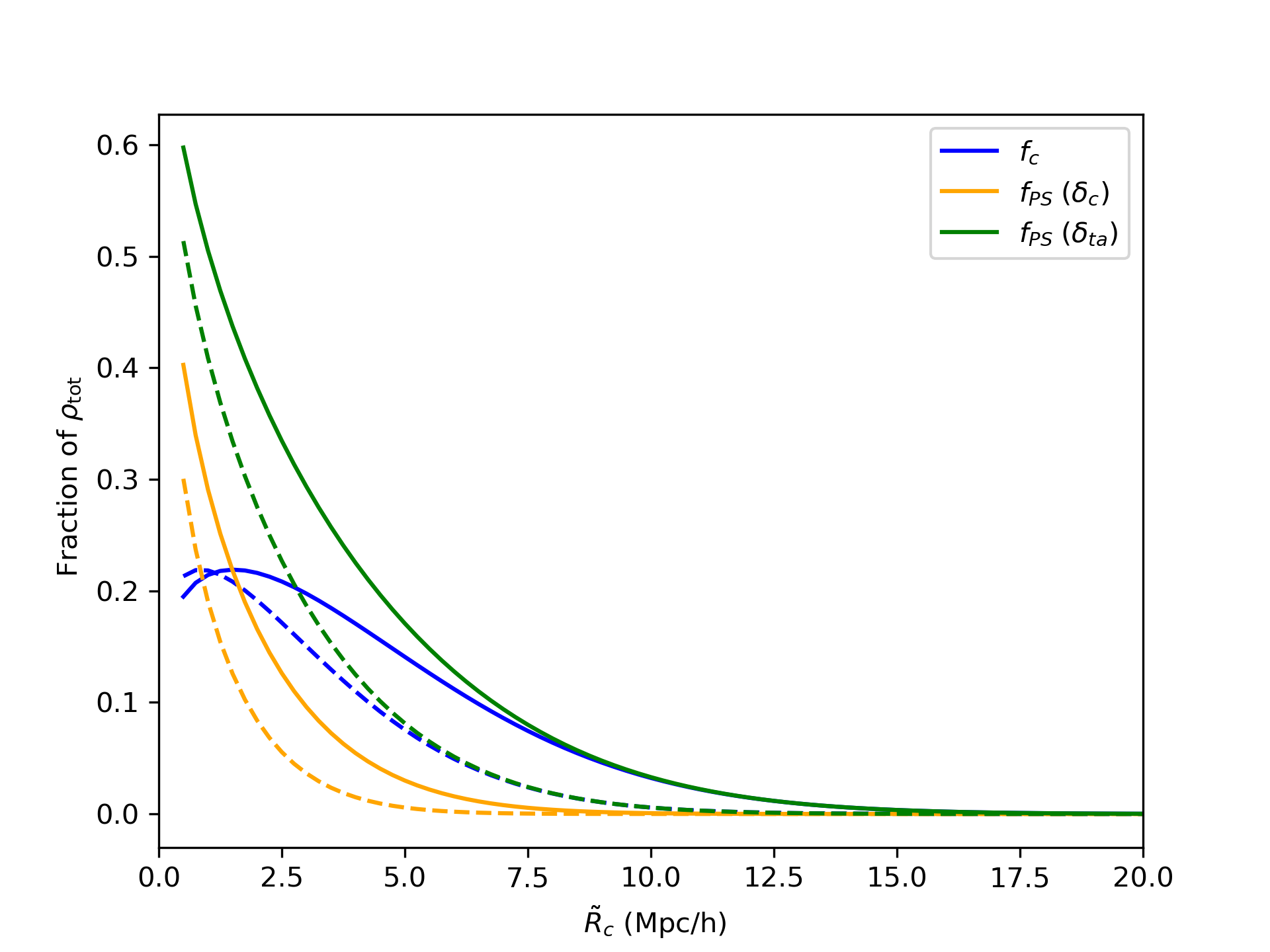
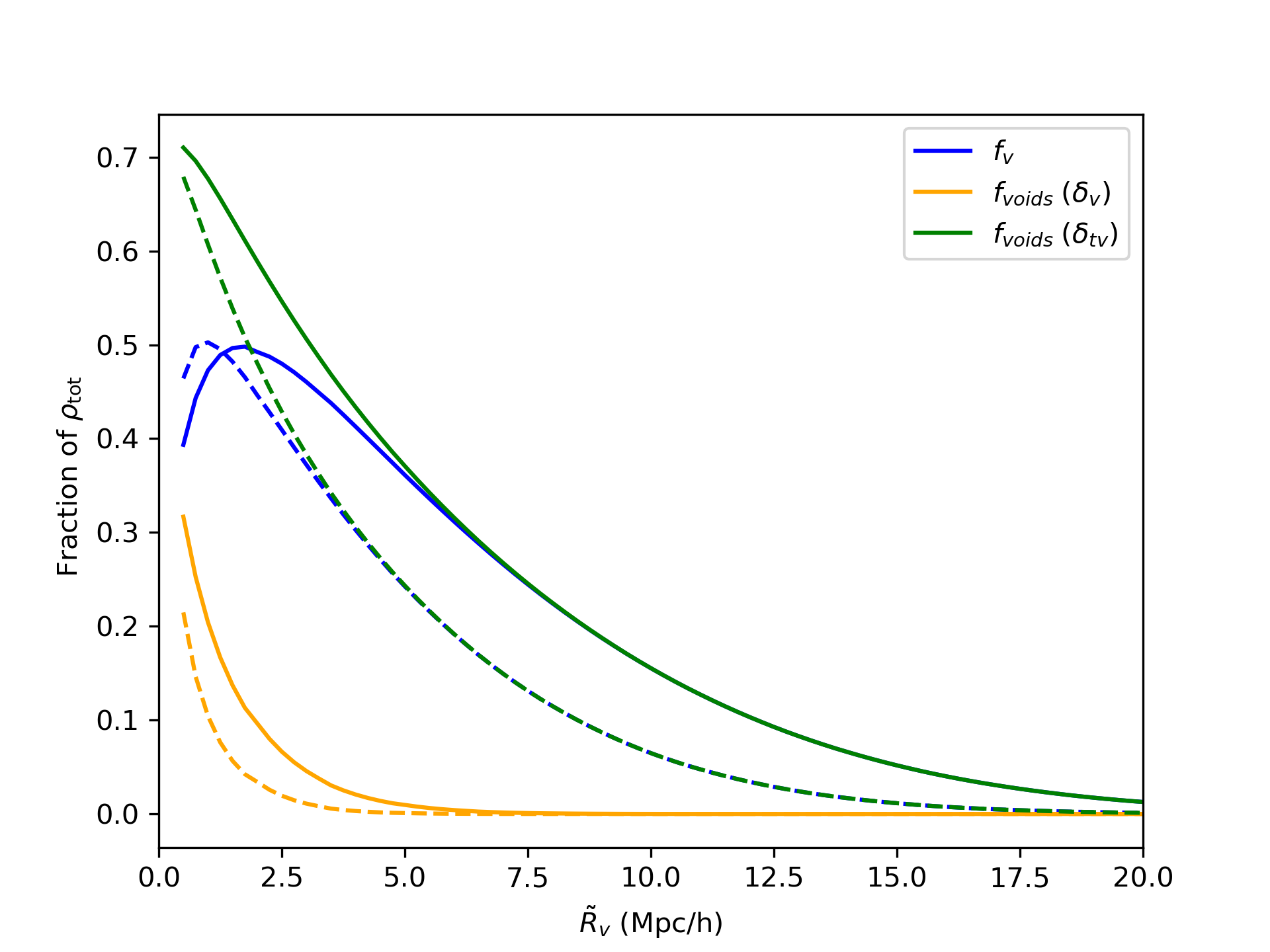
Figure 1: The fraction of non-linear but non-virialized collapsing $f_{\rm{c}}$ (left) and expanding (right) regions $f_{\rm{v}}$ as a function of their minimum radii (blue), together with the fraction of non-linear (green) and virialized (orange) objects, as predicted by Eqs. (10) and (11). Solid lines are computed at $z=0$ and dashed lines at $z=0.5$.

Using the above definitions, we formulate the following ansatz for the energy densities entering Eq. (1)

$$\rho_{\rm{d}}=\rho_{\rm{tot}}\left(1-f_{\rm{v}}-f_{\rm{c}}\right)\;,\quad\rho_{\rm{c}}=\rho_{\rm{tot}}f_{\rm{c}}\;,\quad\rho_{\rm{v}}=\rho_{\rm{tot}}f_{\rm{v}}\;.$$ (12)

II.2 The source terms $C(t)$ and $V(t)$

Given the abundances in Eq. (12), the background dynamics of model is fully specified by the coupling functions $C\left(t\right)$, $V\left(t\right)$ and the EoS parameters $w_{\rm{c}}$ and $w_{\rm{v}}$. The former appear as source terms in the continuity equations, and can be derived from the ansatz of Eq. (12) together with Eqs. (2) and (4). It is convenient to combine both in a single interacting term $Q\left(t\right)\equiv C\left(t\right)+V\left(t\right)$ given by

$${Q}=\left[\dot{f}_{\rm c}+\dot{f}_{\rm v}+3Hw_{\rm{tot}}\left(1-f_{\rm v}-f_{\rm c}\right)\right]\rho_{\rm{tot}}\;.$$ (13)

II.3 Spherical collapse ansatz for $w_{\rm{tot}}$

Our next assumption is that $\rho_{\rm{tot}}$ can be written as

$$c^{2}\rho_{\rm{tot}}=c^{2}\left(\rho_{\rm{dust}}+\rho_{\rm{nl}}\right)\equiv\frac{M_{\rm{dust}}c^{2}+M_{\rm{nl}}c^{2}+\sum_{i}E_{i}^{\;\rm{nl}}}{V}\;,$$ (14)

where we have defined the total masses contained in dust and non-linear structures $M_{\rm{dust}}$ and $M_{\rm{nl}}$, and the internal energies of the latter $E_{i}^{\rm{nl}}$.

Following the spirit of the PS formalism, we compute $E_{i}$ using the spherical collapse model. In virtue of the Birkhoff’s theorem, each spherical region evolves independently and is described by a spatially curved FLRW metric. Following Weinberg [54], the curvature $K_{i}$ associated to a spherical region of initial radius $R(t_{0})$, density perturbation $\delta(t_{0})$ and total mass $M_{i}$ is given by

$$c^{2}K_{i}=\frac{10}{3}M_{i}G\frac{\delta(t_{0})}{R(t_{0})}\;,$$ (15)

to which we associate an internal energy

$$E_{i}=-\frac{3}{8\pi G}\frac{c^{4}K_{i}}{R^{2}}\frac{V_{i}}{R^{2}_{i}}=-\frac{5}{3}M_{i}c^{2}\delta(t)\frac{R_{i}(t)}{\bar{R}(t)}\;,$$ (16)

where $V_{i}$ is the volume of the sphere and $\bar{R}(t)$ the radius that it would have if it was expanding with the background. The spherical collapse model predicts that

$$\frac{R_{i}(t)}{\bar{R}(t)}=\begin{cases}\left[\frac{9}{2}\frac{\left(\theta-\sin{\theta}\right)^{2}}{\left(1-\cos{\theta}\right)^{3}}\right]^{-\frac{1}{3}}\;\;\rm{if}\;\delta>0\;,\\ \left[\frac{9}{2}\frac{\left(\sinh{\theta}-\theta\right)^{2}}{\left(\cosh{\theta}-1\right)^{3}}\right]^{-\frac{1}{3}}\;\rm{if}\;\delta<0\;,\end{cases}$$ (17)

where $t$ and $\theta$ are related by $t(\theta)\propto(\theta-\sin{\theta})$ or $(\sinh{\theta}-\theta)$ for overdense and underdense regions respectively.

Loosely speaking, our definition of internal energy Eq. (16) implies that Eq. (14) becomes the average of the expansion rates of the background and of the non-linearly expanding or contracting spherical regions.

To proceed further, we have to suitably define the terms $M_{\rm{nl}}$, $M_{\rm{dust}}$ (and their sum $M_{\rm{tot}}$) appearing in Eq. (14). A sensible choice is

$$M_{\rm{nl}}\equiv\sum_{i}M_{i}\;,\qquad M_{i}=\frac{4\pi}{3}\rho_{\rm{tot}}R^{3}_{i}\;,$$ (18)

where we have defined the mass $M_{i}$ contained in each spherical region as the amount of total density $\rho_{\rm{tot}}$ within their volume. An important remark is in order: since $\rho_{\rm{tot}}$ is not pressureless, the mass in these objects is non-conserved, $\dot{M}_{i}\neq 0$. Following the PS formalism we can convert the sum into an integral

$$\frac{M_{\rm{nl}}}{V}\equiv\int_{\tilde{R}_{c}}^{\infty}dR\;\frac{df_{c}}{dR}\frac{M_{i}}{V_{i}}+\int_{\tilde{R}_{v}}^{\infty}dR\;\frac{df_{v}}{dR}\frac{M_{i}}{V_{i}}=\rho_{\rm{tot}}\left(f_{v}+f_{c}\right)\;,$$ (19)

where the phenomenological parameters $\tilde{R}_{c}$ and $\tilde{R}_{v}$ fix the minimum scale of collapsing and expanding regions contributing to backreaction effects. Notice that the above implies that the total mass in dust should be identified with

$$\frac{M_{\rm{dust}}}{V}\equiv\rho_{\rm{tot}}-\frac{M_{\rm{nl}}}{V}-\frac{\sum_{i}E_{i}}{Vc^{2}}\;.$$ (20)

In a similar fashion, the sum of the internal energies becomes

$$\begin{split}\sum_{i}&\frac{E_{i}}{V}=\int_{\tilde{R}_{c}}^{\infty}dR\left[\frac{dn_{\rm{{PS}}}(\delta_{c})}{dR}E_{i}\left(\delta_{c}\right)-\frac{dn_{\rm{{PS}}}(\delta_{ta})}{dR}E_{i}\left(\delta_{ta}\right)\right]\\ \;&+\int_{\tilde{R}_{v}}^{\infty}dR\left[\frac{dn_{\rm{{voids}}}(\delta_{v})}{dR}E_{i}\left(\delta_{v}\right)-\frac{dn_{\rm{{voids}}}(\delta_{tv})}{dR}E_{i}\left(\delta_{tv}\right)\right]\;,\end{split}$$ (21)

where $dn_{\rm{PS}}/dR$ and $dn_{\rm{voids}}/dR$ are the differential number densities of collapsing and expanding regions of radius $R$.

The time derivative of Eq. (14) is

$$\frac{\dot{\rho}_{\rm{tot}}}{\rho_{\rm{tot}}}=\frac{\dot{M}_{\rm{tot}}}{M_{\rm{tot}}}-\frac{\dot{V}}{V}+\frac{\left(\frac{\sum_{i}\dot{E}_{i}}{M_{\rm{tot}}}-\frac{\sum_{i}E_{i}}{M_{\rm{tot}}}\frac{\dot{M}_{\rm{tot}}}{M_{\rm{tot}}}\right)}{1+\frac{\sum_{i}E_{i}}{M_{\rm{tot}}}}\;,$$ (22)

from which, assuming that the total mass in the Universe $M_{\rm{tot}}$ is conserved, we can compute the equation of state parameter of the fluid $w_{\rm{tot}}$ using Eq. (5)

$$w_{\rm{tot}}=-\frac{1}{3H\rho_{\rm{tot}}}\frac{\sum_{i}\dot{E}_{i}}{V}\;.$$ (23)

Notice that for $E_{i}=0$ we have $\frac{M_{\rm{nl}}}{M_{\rm{dust}}}=\frac{\rho_{\rm{nl}}}{\rho_{\rm{dust}}}$ and $w_{\rm{tot}}=0$, in agreement with the fact that if $\rho_{\rm{nl}}$ has no internal energy, then there is no difference between the total energy density in rest mass and $\rho_{\rm{tot}}c^{2}$.

A direct consequence of Eqs. (12) and (13) is that the fraction of energy density contained in the non linear structures at a given redshift depends on their minimum scales $R_{v}$, $R_{c}$, and that the equation of state parameter of the total matter fluid depends non-trivially on the abundances of the non-linear species and their time evolution. Notice that the cosmological principle makes it unlikely to have strong density perturbations on large scales, and therefore $f_{\rm v}$ and $f_{\rm c}$ decay exponentially for large values of $R_{i}$, thus recovering the standard $\Lambda$CDM model in this limit.

II.4 Impact of the effective fluid on the growth of perturbations

Eqs. (1)-(4) effectively describe an interacting DM-DE model with $\rho_{\rm{DE}}=\Lambda+\rho_{\rm{c}}+\rho_{\rm{v}}$. Since $\rho_{\rm{c}}$ and $\rho_{\rm{v}}$ and are a purely phenomenological description of the impact of the clustering of dust on the background evolution, and have no physical meaning at a fluid-element level, we assume that (just like $\Lambda$) they do not cluster. Including the interaction term, the perturbation equations for the dust fluid in the Newtonian gauge and the sub-horizon limit become [55]:

$$\dot{\delta}+\theta=\frac{Q}{\rho_{\rm tot}}\left(\delta-\frac{\delta Q}{Q}\right)\,,$$ (24)

$$\dot{\theta}+H\theta+\Delta\phi=0\,,$$ (25)

where $\delta$ is the density contrast, $\theta$ is the divergence of the spatial 3-velocity, $\phi$ is the gravitational potential and $\delta Q$ the perturbation of the coupling term. As it is customary, we also neglect perturbations of the Hubble rate in the sub-horizon limit [56]. Linearizing Eq. (13) around the background evolution and neglecting perturbations of the term within the square brackets, one obtains $\delta Q\approx Q\delta$. Under these hypotheses, we obtain

$$\ddot{\delta}+2H\dot{\delta}-4\pi G\rho_{\rm{d}}\delta=0\;.$$ (26)

It is important to note that, although Eq. (26) retains the same form as in the $\Lambda$CDM model, the evolution of perturbations is now influenced by the quantities $H$ and $\rho_{\rm{d}}=\rho_{\rm{tot}}\left(1-f_{\rm{v}}-f_{\rm{c}}\right)$. We conclude that, in order to understand the behaviour of the model, we need to solve numerically the system of Eqs. (1),(5) and (26) under the hypotheses $\eqref{ansatz1}$, (14), (18) and (19).

III Numerical analysis

Eqs. (1),(5) predict the same expansion history as a $\Lambda$CDM cosmology until relatively low-redshift. We numerically integrate them together with Eq. (26) using the Boltzmann solver CLASS [57] to obtain the initial conditions at redshift $z_{i}=20$, and assume that the transfer function is unchanged. For illustrative purposes, unless otherwise stated, all our plots are obtained by fixing the initial conditions for the Eqs. (1),(5) and (26) at $z_{i}$ to the flat $\Lambda$CDM cosmology best fit (TT,TE,EE+lowE) from Planck 2018 [1].

III.1 Phenomenology

Different choices of $\tilde{R}_{c}$ and $\tilde{R}_{v}$ result in a quite rich phenomenology. Intuitively, $\rho_{c}$ and $\rho_{v}$ should have opposite impact on the behaviour of $\rho_{\rm{tot}}$ due to their opposite contribution to the sign of $\sum_{i}E_{i}$. This expectation is confirmed by Fig. 2, which shows the behaviour of $w_{\rm{tot}}$ for a few choices of the parameters $\tilde{R}_{c}$, $\tilde{R}_{v}$ such that only one between $\rho_{c}$ and $\rho_{v}$ is non-negligible. Voids generally contribute to an effective negative pressure $w_{\rm{tot}}<0$, and collapsing regions to a positive one $w_{\rm{tot}}>0$. This might not occur at low redshifts, since for small values of $\tilde{R}_{c}$ and $\tilde{R}_{v}$ the conversion of non-linearities into virialized objects leads to a sign switch of $\dot{f}_{i}$ and $w_{\rm{tot}}$. The behaviour for general combinations of $\tilde{R}_{c}$ and $\tilde{R}_{v}$, as shown in Fig. 3, permits oscillations in the sign of $w_{\rm{tot}}$.

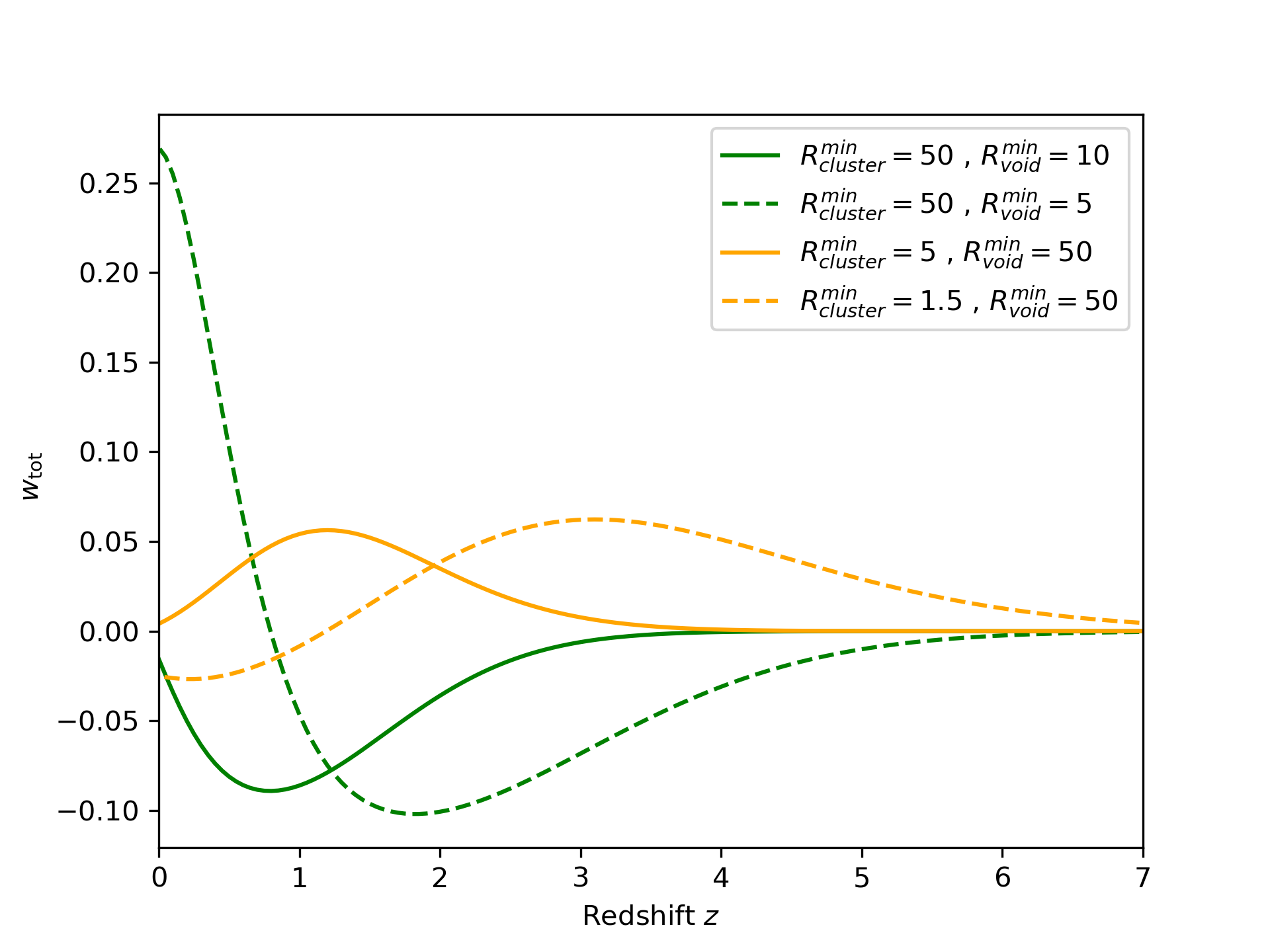
Figure 2: The equation of state parameter of the total matter fluid for different values of $\tilde{R}_{c}$ and $\tilde{R}_{v}$, chosen in such a way that only one specie contributes to the backreaction effects. We see that for sufficiently small $\tilde{R}_{i}$, the conversion of these regions into virialized objects at low redshift lead to a switch in the sign of $w_{\rm{tot}}$.

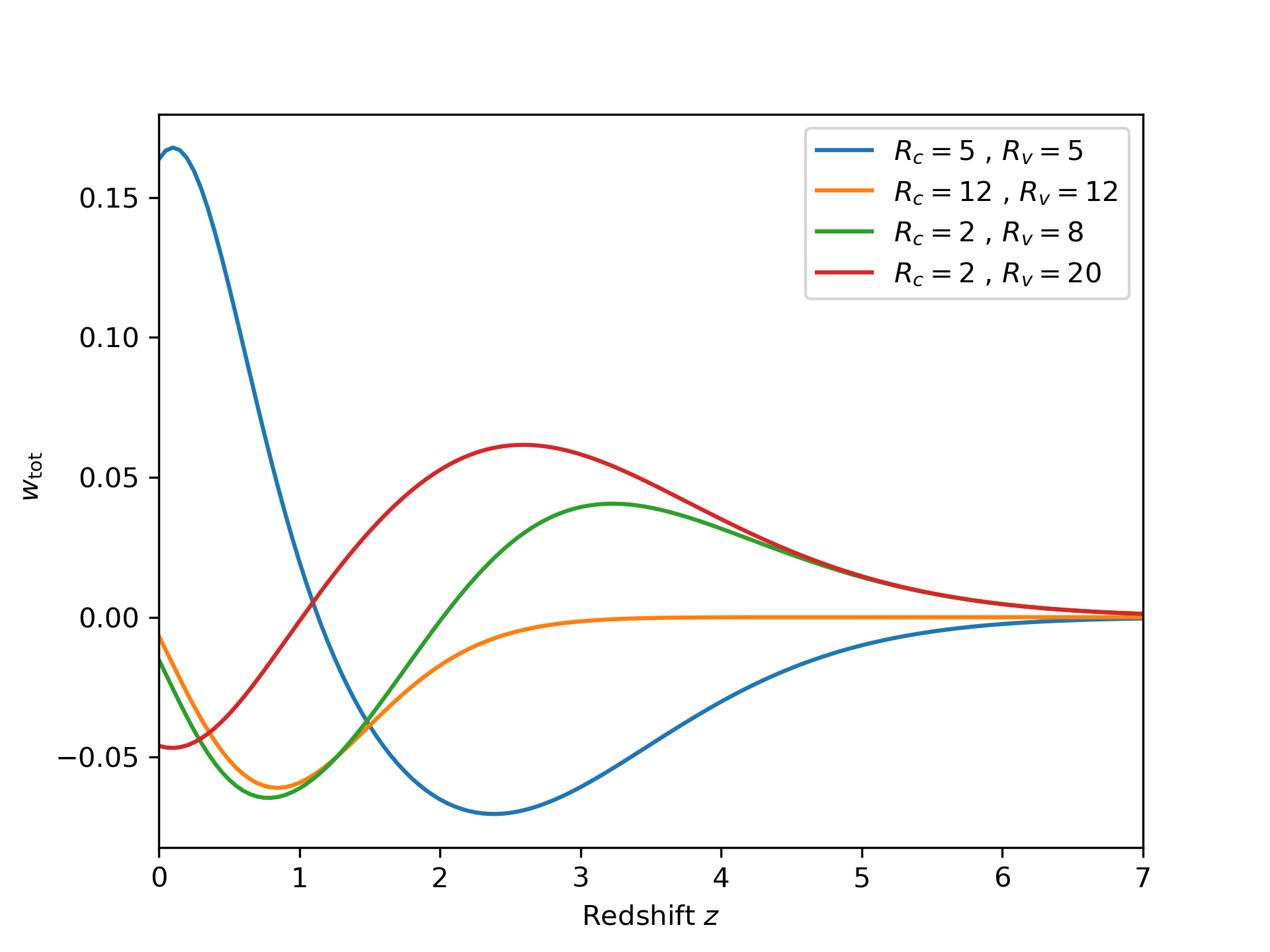
Figure 3: The equation of state parameter of the total matter fluid for a few illustrative choices of $R_{c}$ and $R_{v}$. The model allows for oscillations in $w_{\rm{tot}}$ depending non-trivially on the relative abundance of collapsing and expanding regions at different redshifts.

III.2 Fit to DESY5 SN Ia and growth data

Due to its relevance for the recently suggested evidence for dynamical dark energy [47, 46], we fit the free parameters of the model $\tilde{R}_{\rm{c}}$, $\tilde{R}_{\rm{v}}$ using the latest catalogue of SN Ia from the Dark Energy Survey supernova program (DESY5). We also separately use a sample of uncorrelated measurements of $f\sigma_{8}$ from the latest Sloan Digital Sky Survey Baryon Oscillation Spectroscopic Survey data release (SDSS IV) [58] and peculiar velocity measurements from 6df and SDSS [59, 60]. To assess whether the modified evolution of the matter fluid can alleviate the mismatch between early and late times Universe probes, we fix the initial conditions at redshift $z=20$ to the best fit values for a flat $\Lambda$CDM cosmology from Planck 2018 [1]. For the SN Ia we use the Cobaya [61, 62] MCMC sampler, and for the growth measurements we use the emcee [63].. We impose flat log priors $0<\log{\tilde{R}_{i}}<1.5$. The lower bound is chosen in such a way that we only consider backreaction effects from objects with typical scales larger than $\tilde{R}_{i}\geq 1$ Mpc/h. The upper bound is somewhat arbitrary, but such that deviations from the standard $\Lambda$CDM expansion history and growth of perturbations are negligible (i.e. below $<0.1\%$ percent level). Extending the prior range to higher values of $\tilde{R}_{i}$ has negligible impact on the best fit values.

Fig. 4 shows our exploration of the 2-dimensional parameter space $\tilde{R}_{\rm{c}},\tilde{R}_{\rm{v}}$. The two dataset are quite complementary, with SNe Ia constraining $\tilde{R}_{v}$ and $f\sigma_{8}$ measurements constraining $\tilde{R}_{c}$. Table 1 shows a comparison between the $\chi^{2}$ values obtained for the best fit from Planck $\Lambda$CDM and our model. Fig. 5 compares the Planck 2018 best fit $\Lambda$CDM evolution of $f\sigma_{8}$ and our model’s best fit.

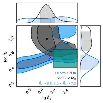
Figure 4: Constraints on the free parameters $\tilde{R}_{c},\tilde{R}_{v}$ for DESY5 SnIa (blue) and $f\sigma_{8}$ measurements from RDS and Peculiar velocities [58, 59, 60]. We see that the datasets are quite complementary, with the former being sensitive mostly to $\tilde{R}_{v}$ and the latter to $\tilde{R}_{c}$. The green box indicates a region of parameter space that could potentially alleviate at the same time the $H_{0}$ and $\sigma_{8}$ tensions (see Fig. 6).

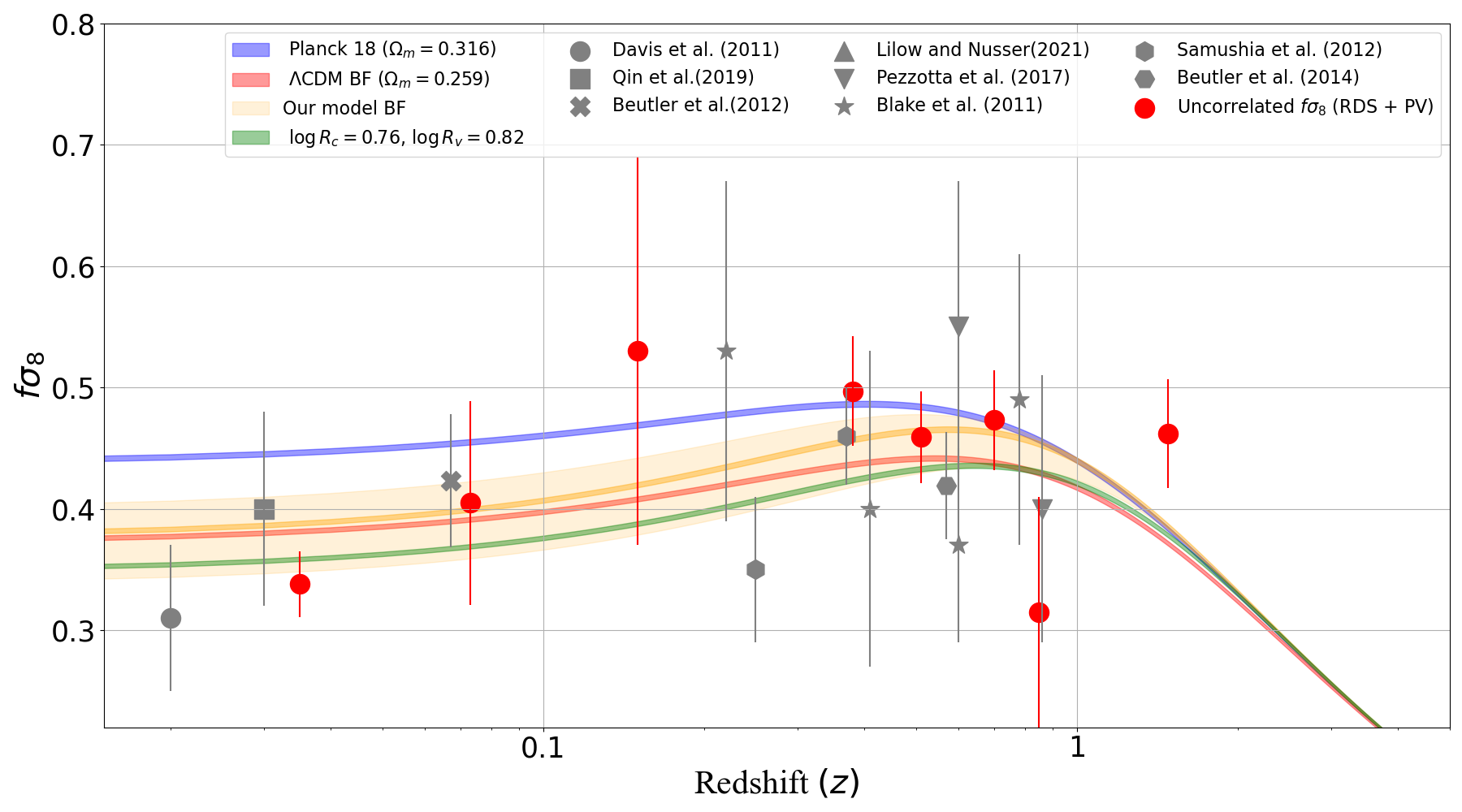
Figure 5: Predictions for the evolution of $f\sigma_{8}$ from Planck 2018 (blue), $\Lambda$CDM best fit (red), our model’s best fit (orange) and with $\tilde{R}_{\rm{v}}$ fixed to the DESY5 peak (green). Red dots indicate the uncorrelated $f\sigma_{8}$ measurements used for the fit [58, 60, 59] and the grey points a collection of correlated measurements from the recent literature [64, 65, 66, 67, 68, 69, 70, 71].

We stress that these results are illustrative, and a more rigorous analysis should consider both datasets together with CMB data, leaving free to vary the initial conditions on $\Omega_{m}$, $\Omega_{\Lambda}$. On the other hand, our simple exercise shows the healthy phenomenology of the model and its potential to address a few challenges of the standard model.

Table 1: The results of our MCMC parameter exploration of DESY5 and uncorrelated $f\sigma_{8}$ measurements

	$\chi^{2}$			Parameters
	PL18	$\Lambda$CDM	Our model	log $\tilde{R}_{\rm c}$	log $\tilde{R}_{\rm v}$
DESY5 SN (1735${}^{{\dagger}}\ d.o.f$)	1653.88	1649.88	1648.22	$0.83^{+0.43}_{-0.58}$	$0.66^{+0.15}_{-0.16}$
RSD + PV (8 $d.o.f$)	21.9	11.7	11.4	$0.75^{+0.19}_{-0.15}$	$1.15^{+0.24}_{-0.22}$

^† The low $\chi^{2}/$d.o.f is due to the treatment of likely contaminants in the DESY5 sample which have had their uncertainties inflated. As a result, the effective number of data points is approximated by $\sum P_{\mathrm{B}(\mathrm{Ia})}=1735$ rather than the total number of data points, 1829.

III.3 Impact on cosmological tensions

Fig. 6 shows the variations of $H_{0}$ and $\sigma_{8}$ with respect to the best fit Planck 2018 $\Lambda$CDM cosmology as a function of $\tilde{R}_{c}$ and $\tilde{R}_{v}$. Since we assume that $\rho_{\rm{c}}$ and $\rho_{\rm{v}}$ do not cluster, the value of $\sigma_{8}$ is generally lower than in $\Lambda$CDM. Interestingly, there is a region of the parameter space predicting both a higher $H_{0}$ and a lower $\sigma_{8}$, potentially alleviating both tensions at the same time.

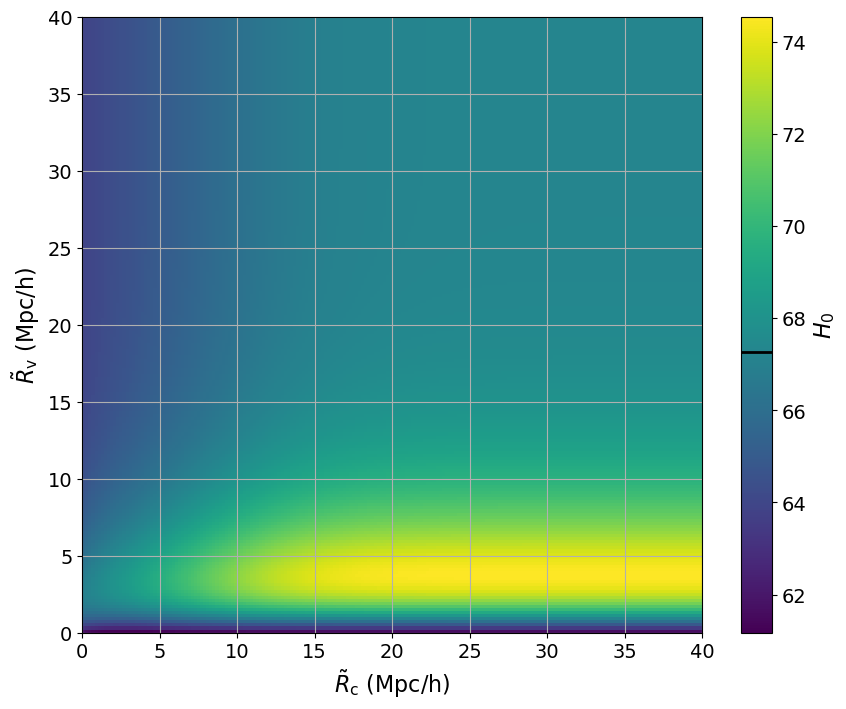
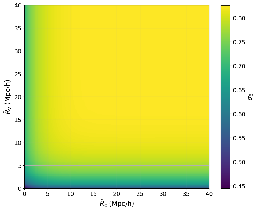
Figure 6: Variations in the value of the cosmological parameters $H_{0}$ (left) and $\sigma_{8}(z=0)$ (right) with respect to the reference $\Lambda$CDM cosmology from the Planck 2018 best fit. Interestingly, there is a region of the parameter space (around $\tilde{R}_{c}>8$ and $2.5<\tilde{R}_{v}<7.5$ Mpc/h) that could potentially alleviate both tensions at the same time. In the $H_{0}$ panel, the black line on the color bar denotes the $\Lambda$CDM inferred value from the initial conditions fixed at $z=20$. The corresponding one in the $\sigma_{8}$ panel is at the top of the color bar.

In Fig. 7 we show the fractional change in the expansion history $H(z)$, $\sigma_{8}$ and the total matter density $\Omega_{m}$ for the best fit parameters $\tilde{R}_{c},\tilde{R}_{v}$ from Table 1. We also plot the evolution of the different energy density contributions entering in the modified Friedmann equation (1). Notice that for the chosen best fit values, the most abundant specie in the Universe at low redshift is the effective void fluid $\rho_{v}$.

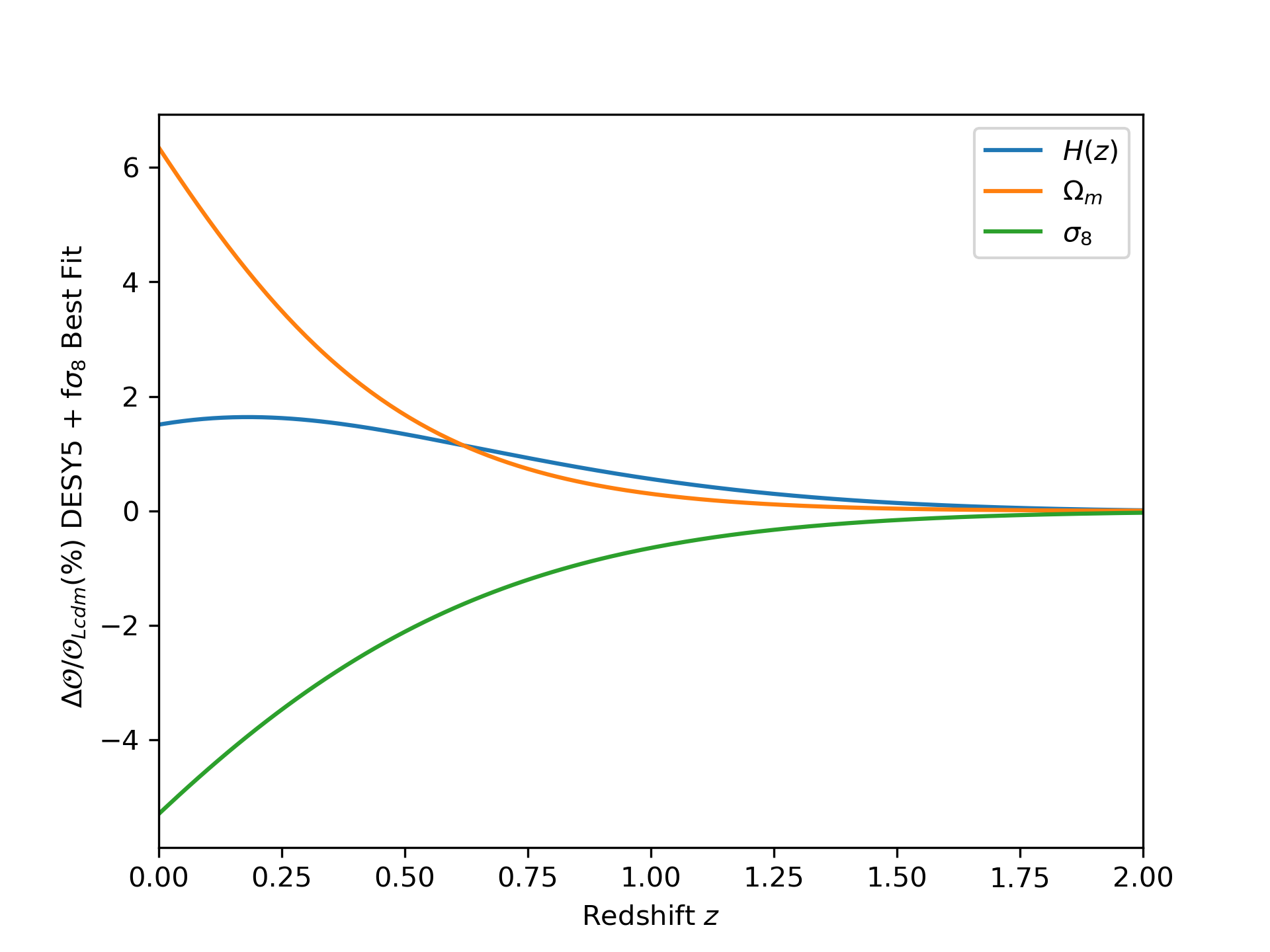
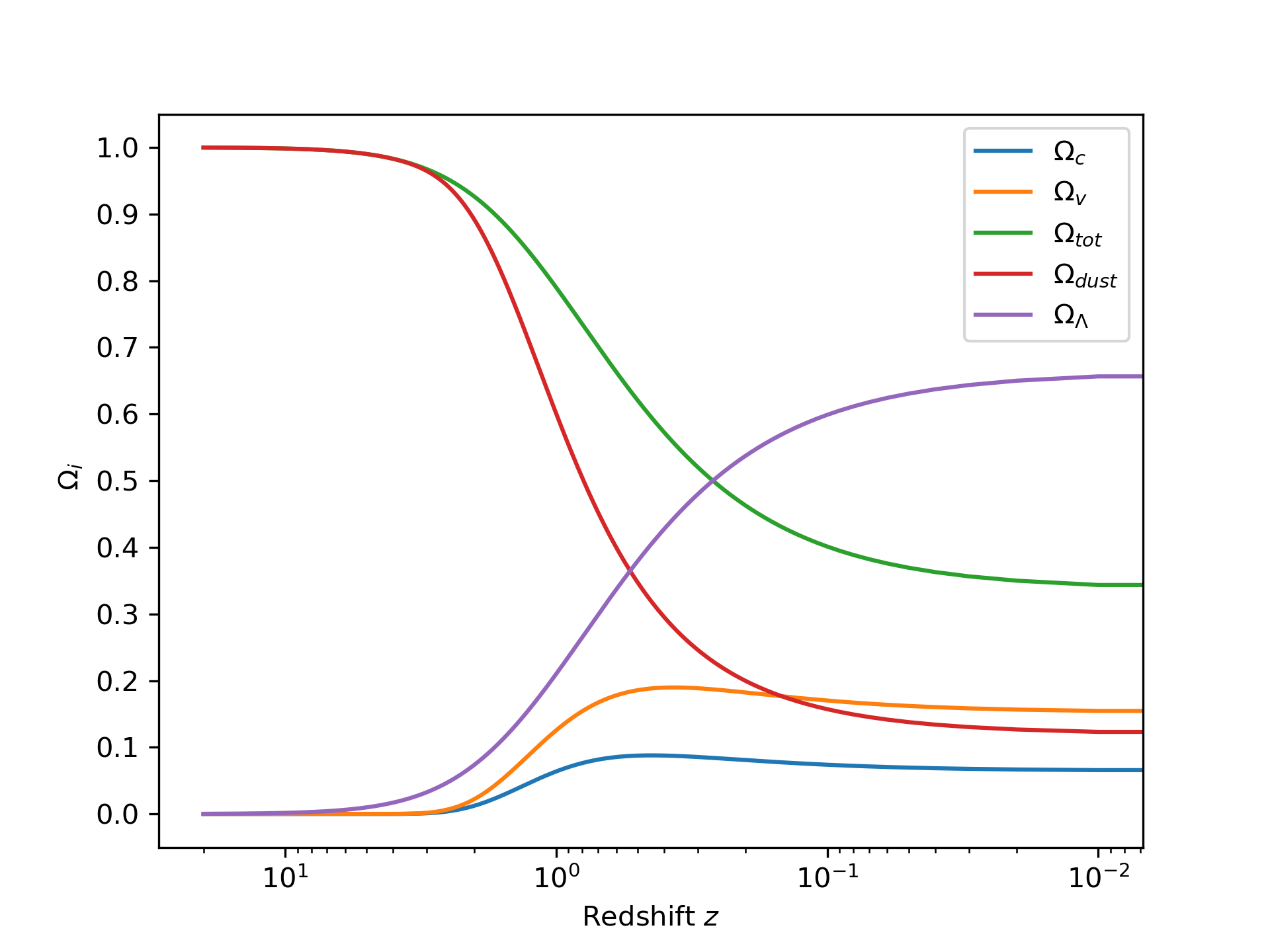
Figure 7: Left: Comparison between the cosmological behaviour of our model for the best fit parameters from Table 1 and the fiducial Planck 2018 flat $\Lambda$CDM cosmology. Right: The contributions of the various fluids entering the Friedmann equation as a function of time for the best fit model of Table 1.

IV Discussion

This letter proposes a new phenomenological description of the cosmological backreaction from matter inhomogeneities inspired by models of interacting DM-DE. We introduce a coupling between the matter non-linearities and the “dust” at the background level, describing the conversion of matter fluctuations into large scale structures. We make use of the Press Schechter formalism to quantify the number of non-linearly evolving regions in the Universe that have not virialized yet. Following the spirit of the PS ansatz, we treat them as if they were spherical, and evolving independently in virtue of Birkhoff theorem. It is worth stressing that our proposal is not a Newtonian backreaction model. Indeed, as shown in Eqs. (7), the Buchertian averaged spatial curvature ${}^{3}\mathcal{R}$ is in general non-vanishing.

Similarly to other backreaction proposals [29], our model depends on a somewhat arbitrary choice of averaging scales. Common sense suggests that sufficiently small regions should have no impact on the background evolution of the Universe. This simple argument is backed up by several investigations in the literature [41, 43, 38, 73], which have shown that backreaction effects from virialized objects in a Newtonian framework are completely negligible. For this reason, we focus our attention to non-virialized regions with linear scales $\geq 1\;\rm{Mpc/h}$, but leave otherwise free the additional parameters of the model, $\tilde{R}_{c}$ and $\tilde{R}_{v}$, determining the minimum size of the regions considered relevant for backreaction effects.

As shown in Fig. 3, different combinations of $\tilde{R}_{i}$ result in a quite rich phenomenology. Broadly speaking, the model features a different expansion history with respect to a vanilla $\Lambda$CDM at relatively low redshift, depending on the relative abundance of collapsing and expanding non-linear regions. Note that the non-linear effective fluid is, by its own nature, a transient phenomena, since the non-linear objects will eventually virialize (i.e. undergo shell-crossing) and effectively become dust once again. If the minimum size of the regions is sufficiently small, the decay becomes efficient before present day, leading to an interesting phenomenology. Fig. 3 shows that smaller values of $\tilde{R}_{i}$ lead to a switch in the sign of the equation of state parameter $w_{\rm{tot}}$ at $z\ll 1$. This is explained by the sign switch of $C(t)+V(t)$ in Eq. (13) occurring for decaying $f_{v}$ and $f_{c}$.

The recent indications for dynamical dark energy [47, 46] occurs when simultaneously combining SnIa, BAO and CMB information. In a nutshell, the disagreement between matter density predictions from high- and low-redshift probes points towards a preference for dynamical dark energy, which can reconcile the data sets thanks to its additional free parameters. However, a similar phenomenology is also naturally achieved in our model. As shown in Table 1, our model’s best fit to the DESY5 SnIa alone improves the fit over the best fit Planck $\Lambda$CDM by $\Delta\chi^{2}\sim-6$, and is comparable to the $\Lambda$CDM best fit to the SnIa alone ($\Omega_{m}=0.352\pm 0.017$ with $\chi^{2}/\mathrm{d.o.f}=1649/1734$), while maintaining an early-times matter density fixed by construction to the Planck value.

Summarising, this work proposes an innovative two-parameters extension of the $\Lambda$CDM. Our model is equivalent to an interacting DM-DE scenario, and aims to describe backreaction effects from the cosmic web. The resulting phenomenology can potentially address a few major challenges of the concordance model and provide insightful clues to the “fitting problem” in Cosmology [74].

V Acknowledgments

It is a pleasure to thank Timothy Clifton, Tamara Davis, Asta Heinesen, Cullan Howlett, Valerio Marra, Oliver Piattella, Khaled Said and Sunny Vagnozzi for their useful comments and suggestions. LG and RC acknowledge the support of an Australian Research Council Australian Laureate Fellowship (FL180100168) funded by the Australian Government. RvM is suported by Fundação de Amparo à Pesquisa do Estado da Bahia (FAPESB) grant TO APP0039/2023.

Appendix A Press Schechter formalism

Collapsing objects

In its simplest formulation, the Press Schechter formalism assumes that the linear density contrast smoothed on spheres of radius $R$ is a Gaussian random field with variance

$$\sigma^{2}(t,R)\equiv\langle\delta^{2}\rangle=\int_{0}^{\infty}d\ln{k}\frac{k^{3}}{2\pi^{2}}P(t,k)|W(k,R)|^{2}\;,$$ (27)

where $P(k,t)$ is the linear matter power spectrum, and $W(k,R)$ is a spherical top-hat filter in Fourier space

$$W(k,R)=\frac{3}{\left(kR\right)^{3}}\left[\sin{\left(kR\right)}-kR\cos{\left(kR\right)}\right]\;.$$ (28)

It follows that the probability for a spherical volume of space to have density contrast $\delta_{X}$ is given by

$$P(\delta_{X})=\frac{1}{\sqrt{2\pi}\sigma_{R}}e^{-\frac{1}{2}\left(\frac{\delta_{X}}{\sigma_{R}}\right)^{2}}\;,$$ (29)

which can be used to predict the expected abundance of virialized objects of mass $M$ at any given time, the so-called halo mass function. The fraction of total matter contained in these objects is obtained integrating the above probability above the threshold for virialization $\delta_{c}=1.68$ predicted by the spherical collapse model[52, 53]

$$f_{\rm{PS}}\left(>\delta_{c}\right)=2\int_{\delta_{c}}^{\infty}d\delta\;P\left(\delta\right)=1-\rm{erf}\left(\frac{\delta_{c}}{\sqrt{2}\sigma_{R}}\right)\;,$$ (30)

where the factor $2$ multiplying the integral has been introduced by PS to correctly normalize the above probability, but lacked a rigorous motivation. It has been shown in Ref. [49] how this factor emerges naturally within the excursion set theory formalism to account for the cloud-in-a-cloud problem. From Eq. (30) it is possible to define the halo mass function

$$\frac{dn_{\rm{PS}}}{dM}=-\frac{df_{\rm{{PS}}}}{dM}\frac{\bar{\rho}}{M}\;,$$ (31)

giving the fraction of objects of a given mass $M(R)$ at redshift $z$.

Voids

The extension of the excursion formalism for the distribution of voids has been pioneered in Ref. [50], where it has been recognised that whereas it is possible to have smaller haloes within a virialized void region, the opposite is unphysical. Given two threshold barriers for the virialization of overdensities $\delta_{c}$ and underdensities $\delta_{v}$, the following approximation for the number density of voids as a function of their (linearly extrapolated) radius was obtained in [51]

$$\frac{df_{\rm{ln}\sigma}}{dR}=\begin{cases}\sqrt{\frac{2}{\pi}}\frac{|\delta_{v}^{\rm{lin}}|}{\sigma}e^{-\left(\frac{\delta_{v}^{\rm{lin}}}{\sqrt{2}\sigma}\right)^{2}}\quad\quad\quad\rm{for}\;\;x\leq 0.276\;,\\ 2\sum_{j=1}^{4}e^{-\frac{(j\pi x)^{2}}{2}}j\pi x^{2}\sin\left(j\pi\mathcal{D}\right)\;\;\rm{for}\;\;x>0.276\;,\end{cases}$$ (32)

where we have defined

$$\mathcal{D}=\frac{|\delta_{v}^{\rm{lin}}|}{|\delta_{v}^{\rm{lin}}|+\delta_{c}^{\rm{lin}}}\;,\qquad x=\frac{\mathcal{D}}{|\delta_{v}^{\rm{lin}}|}\sigma\;.$$ (33)

The fraction of voids with radius larger than $\tilde{R}$ is therefore easily obtained integrating the above

$$f_{\rm{voids}}\equiv\int_{\tilde{R}}^{\infty}\frac{dR}{R}\;\frac{df_{\rm{ln}\sigma}}{dR}\frac{d\ln\sigma^{-1}}{d\ln{R}}\;,$$ (34)

whereas the number density of voids of radius $R$ can be written

$$\frac{dn_{\rm{void}}}{dR}\equiv\frac{df}{d\ln\sigma}\frac{d\ln\sigma^{-1}}{d\ln R_{\rm{lin}}}\frac{d\ln{R_{\rm{lin}}}}{d\ln{R}}\frac{\bar{\rho}}{M}\;,$$ (35)

where $R_{\rm{lin}}(R)$ and its Jacobian have been included to conserve the total volume fraction in voids rather than their numbers [51].

References

- [1] N. Aghanim et al. Planck 2018 results. VI. Cosmological parameters. Astron. Astrophys., 641:A6, 2020. [Erratum: Astron.Astrophys. 652, C4 (2021)]. arXiv:1807.06209, doi:10.1051/0004-6361/201833910.
- [2] A. Jenkins, C. S. Frenk, Simon D. M. White, J. M. Colberg, S. Cole, August E. Evrard, H. M. P. Couchman, and N. Yoshida. The Mass function of dark matter halos. Mon. Not. Roy. Astron. Soc., 321:372, 2001. arXiv:astro-ph/0005260, doi:10.1046/j.1365-8711.2001.04029.x.
- [3] Romain Teyssier. Cosmological hydrodynamics with adaptive mesh refinement: a new high resolution code called RAMSES. Astron. Astrophys., 385:337–364, 2002. arXiv:astro-ph/0111367, doi:10.1051/0004-6361:20011817.
- [4] Volker Springel et al. Simulating the joint evolution of quasars, galaxies and their large-scale distribution. Nature, 435:629–636, 2005. arXiv:astro-ph/0504097, doi:10.1038/nature03597.
- [5] Mark Vogelsberger, Shy Genel, Volker Springel, Paul Torrey, Debora Sijacki, Dandan Xu, Gregory F. Snyder, Dylan Nelson, and Lars Hernquist. Introducing the Illustris Project: Simulating the coevolution of dark and visible matter in the Universe. Mon. Not. Roy. Astron. Soc., 444(2):1518–1547, 2014. arXiv:1405.2921, doi:10.1093/mnras/stu1536.
- [6] Julian Adamek, David Daverio, Ruth Durrer, and Martin Kunz. gevolution: a cosmological N-body code based on General Relativity. JCAP, 07:053, 2016. arXiv:1604.06065, doi:10.1088/1475-7516/2016/07/053.
- [7] Julian Adamek, Cristian Barrera-Hinojosa, Marco Bruni, Baojiu Li, Hayley J. Macpherson, and James B. Mertens. Numerical solutions to Einstein’s equations in a shearing-dust Universe: a code comparison. Class. Quant. Grav., 37(15):154001, 2020. arXiv:2003.08014, doi:10.1088/1361-6382/ab939b.
- [8] Hayley J. Macpherson and Asta Heinesen. Luminosity distance and anisotropic sky-sampling at low redshifts: A numerical relativity study. Phys. Rev. D, 104:023525, 2021. [Erratum: Phys.Rev.D 104, 109901 (2021)]. arXiv:2103.11918, doi:10.1103/PhysRevD.104.023525.
- [9] Spencer J. Magnall, Daniel J. Price, Paul D. Lasky, and Hayley J. Macpherson. Inhomogeneous cosmology using general relativistic smoothed particle hydrodynamics coupled to numerical relativity. Phys. Rev. D, 108(10):103534, 2023. arXiv:2307.15194, doi:10.1103/PhysRevD.108.103534.
- [10] Michael J. Williams, Hayley J. Macpherson, David L. Wiltshire, and Chris Stevens. First investigation of void statistics in numerical relativity simulations. preprint, 3 2024. arXiv:2403.15134.
- [11] Cristian Barrera-Hinojosa and Baojiu Li. GRAMSES: a new route to general relativistic -body simulations in cosmology. Part I. Methodology and code description. JCAP, 01:007, 2020. arXiv:1905.08890, doi:10.1088/1475-7516/2020/01/007.
- [12] Eduardo Quintana-Miranda, Pierluigi Monaco, and Luca Tornatore. grgadget: an N-body TreePM relativistic code for cosmological simulations. Mon. Not. Roy. Astron. Soc., 522(4):5238–5253, 2023. arXiv:2301.11854, doi:10.1093/mnras/stad1174.
- [13] Christian Sicka, Thomas Buchert, and Martin Kerscher. Back reaction in cosmological models. Lect. Notes Phys., 546:375, 2000. arXiv:astro-ph/9907137.
- [14] George F. R. Ellis and Thomas Buchert. The Universe seen at different scales. Phys. Lett. A, 347:38–46, 2005. arXiv:gr-qc/0506106, doi:10.1016/j.physleta.2005.06.087.
- [15] Valerio Marra, Edward W. Kolb, Sabino Matarrese, and Antonio Riotto. On cosmological observables in a swiss-cheese universe. Phys. Rev. D, 76:123004, 2007. arXiv:0708.3622, doi:10.1103/PhysRevD.76.123004.
- [16] Stephen R. Green and Robert M. Wald. A new framework for analyzing the effects of small scale inhomogeneities in cosmology. Phys. Rev. D, 83:084020, 2011. arXiv:1011.4920, doi:10.1103/PhysRevD.83.084020.
- [17] Thomas Buchert and Syksy Räsänen. Backreaction in late-time cosmology. Ann. Rev. Nucl. Part. Sci., 62:57–79, 2012. arXiv:1112.5335, doi:10.1146/annurev.nucl.012809.104435.
- [18] Krzysztof Bolejko. Cosmological backreaction within the Szekeres model and emergence of spatial curvature. JCAP, 06:025, 2017. arXiv:1704.02810, doi:10.1088/1475-7516/2017/06/025.
- [19] S. M. Koksbang. Another look at redshift drift and the backreaction conjecture. JCAP, 10:036, 2019. arXiv:1909.13489, doi:10.1088/1475-7516/2019/10/036.
- [20] Thomas Buchert, Pierre Mourier, and Xavier Roy. On average properties of inhomogeneous fluids in general relativity III: general fluid cosmologies. Gen. Rel. Grav., 52(3):27, 2020. arXiv:1912.04213, doi:10.1007/s10714-020-02670-6.
- [21] Akihiro Ishibashi and Robert M. Wald. Can the acceleration of our universe be explained by the effects of inhomogeneities? Class. Quant. Grav., 23:235–250, 2006. arXiv:gr-qc/0509108, doi:10.1088/0264-9381/23/1/012.
- [22] Stephen R. Green and Robert M. Wald. How well is our universe described by an FLRW model? Class. Quant. Grav., 31:234003, 2014. arXiv:1407.8084, doi:10.1088/0264-9381/31/23/234003.
- [23] Stephen R. Green and Robert M. Wald. A simple, heuristic derivation of our ‘no backreaction’ results. Class. Quant. Grav., 33(12):125027, 2016. arXiv:1601.06789, doi:10.1088/0264-9381/33/12/125027.
- [24] Hayley J. Macpherson, Daniel J. Price, and Paul D. Lasky. Einstein’s Universe: Cosmological structure formation in numerical relativity. Phys. Rev. D, 99(6):063522, 2019. arXiv:1807.01711, doi:10.1103/PhysRevD.99.063522.
- [25] Syksy Rasanen. Dark energy from backreaction. JCAP, 02:003, 2004. arXiv:astro-ph/0311257, doi:10.1088/1475-7516/2004/02/003.
- [26] Havard Alnes, Morad Amarzguioui, and Oyvind Gron. An inhomogeneous alternative to dark energy? Phys. Rev. D, 73:083519, 2006. arXiv:astro-ph/0512006, doi:10.1103/PhysRevD.73.083519.
- [27] Tirthabir Biswas, Reza Mansouri, and Alessio Notari. Nonlinear Structure Formation and Apparent Acceleration: An Investigation. JCAP, 12:017, 2007. arXiv:astro-ph/0606703, doi:10.1088/1475-7516/2007/12/017.
- [28] Thomas Buchert. Dark Energy from Structure: A Status Report. Gen. Rel. Grav., 40:467–527, 2008. arXiv:0707.2153, doi:10.1007/s10714-007-0554-8.
- [29] David L. Wiltshire. Average observational quantities in the timescape cosmology. Phys. Rev. D, 80:123512, 2009. arXiv:0909.0749, doi:10.1103/PhysRevD.80.123512.
- [30] Asta Heinesen and Thomas Buchert. Solving the curvature and Hubble parameter inconsistencies through structure formation-induced curvature. Class. Quant. Grav., 37(16):164001, 2020. [Erratum: Class.Quant.Grav. 37, 229601 (2020)]. arXiv:2002.10831, doi:10.1088/1361-6382/ab954b.
- [31] Pierre Fleury, Hélène Dupuy, and Jean-Philippe Uzan. Interpretation of the Hubble diagram in a nonhomogeneous universe. Phys. Rev. D, 87(12):123526, 2013. arXiv:1302.5308, doi:10.1103/PhysRevD.87.123526.
- [32] T. Buchert et al. Is there proof that backreaction of inhomogeneities is irrelevant in cosmology? Class. Quant. Grav., 32:215021, 2015. arXiv:1505.07800, doi:10.1088/0264-9381/32/21/215021.
- [33] Krzysztof Bolejko, M. Ahsan Nazer, and David L. Wiltshire. Differential cosmic expansion and the Hubble flow anisotropy. JCAP, 06:035, 2016. arXiv:1512.07364, doi:10.1088/1475-7516/2016/06/035.
- [34] Leonardo Giani, Cullan Howlett, Khaled Said, Tamara Davis, and Sunny Vagnozzi. An effective description of Laniakea: impact on cosmology and the local determination of the Hubble constant. JCAP, 01:071, 2024. arXiv:2311.00215, doi:10.1088/1475-7516/2024/01/071.
- [35] Theodore Anton and Timothy Clifton. Modelling the emergence of cosmic anisotropy from non-linear structures. Class. Quant. Grav., 40(14):145004, 2023. arXiv:2302.05715, doi:10.1088/1361-6382/acdbfd.
- [36] Timothy Clifton and Neil Hyatt. A Radical Solution to the Hubble Tension Problem. preprint, 4 2024. arXiv:2404.08586.
- [37] Edward W. Kolb, Valerio Marra, and Sabino Matarrese. Cosmological background solutions and cosmological backreactions. Gen. Rel. Grav., 42:1399–1412, 2010. arXiv:0901.4566, doi:10.1007/s10714-009-0913-8.
- [38] Daniel Baumann, Alberto Nicolis, Leonardo Senatore, and Matias Zaldarriaga. Cosmological Non-Linearities as an Effective Fluid. JCAP, 07:051, 2012. arXiv:1004.2488, doi:10.1088/1475-7516/2012/07/051.
- [39] John Joseph M. Carrasco, Mark P. Hertzberg, and Leonardo Senatore. The Effective Field Theory of Cosmological Large Scale Structures. JHEP, 09:082, 2012. arXiv:1206.2926, doi:10.1007/JHEP09(2012)082.
- [40] Matthew Lewandowski, Azadeh Maleknejad, and Leonardo Senatore. An effective description of dark matter and dark energy in the mildly non-linear regime. JCAP, 05:038, 2017. arXiv:1611.07966, doi:10.1088/1475-7516/2017/05/038.
- [41] Thomas Buchert and Jurgen Ehlers. Averaging inhomogeneous Newtonian cosmologies. Astron. Astrophys., 320:1–7, 1997. arXiv:astro-ph/9510056.
- [42] P. J. E. Peebles, Jean-Michel Alimi, and Andre Fuozfa. Phenomenology of the invisible universe. In AIP Conference Proceedings. AIP, 2010. URL: http://dx.doi.org/10.1063/1.3462631, doi:10.1063/1.3462631.
- [43] Valerio Marra and Alessio Notari. Observational constraints on inhomogeneous cosmological models without dark energy. Class. Quant. Grav., 28:164004, 2011. arXiv:1102.1015, doi:10.1088/0264-9381/28/16/164004.
- [44] Viraj A. A. Sanghai and Timothy Clifton. Post-Newtonian Cosmological Modelling. Phys. Rev. D, 91:103532. arXiv:1503.08747, doi:10.1103/PhysRevD.93.089903.
- [45] Elcio Abdalla et al. Cosmology intertwined: A review of the particle physics, astrophysics, and cosmology associated with the cosmological tensions and anomalies. JHEAp, 34:49–211, 2022. arXiv:2203.06142, doi:10.1016/j.jheap.2022.04.002.
- [46] T. M. C. Abbott et al. The Dark Energy Survey: Cosmology Results With ~1500 New High-redshift Type Ia Supernovae Using The Full 5-year Dataset. 1 2024. arXiv:2401.02929.
- [47] A. G. Adame et al. DESI 2024 VI: Cosmological Constraints from the Measurements of Baryon Acoustic Oscillations. 4 2024. arXiv:2404.03002.
- [48] William H. Press and Paul Schechter. Formation of galaxies and clusters of galaxies by selfsimilar gravitational condensation. Astrophys. J., 187:425–438, 1974. doi:10.1086/152650.
- [49] J. R. Bond, S. Cole, G. Efstathiou, and N. Kaiser. Excursion Set Mass Functions for Hierarchical Gaussian Fluctuations. apj, 379:440, October 1991. doi:10.1086/170520.
- [50] Ravi K. Sheth and Rien van de Weygaert. A Hierarchy of voids: Much ado about nothing. Mon. Not. Roy. Astron. Soc., 350:517, 2004. arXiv:astro-ph/0311260, doi:10.1111/j.1365-2966.2004.07661.x.
- [51] Elise Jennings, Yin Li, and Wayne Hu. The abundance of voids and the excursion set formalism. Mon. Not. Roy. Astron. Soc., 434:2167, 2013. arXiv:1304.6087, doi:10.1093/mnras/stt1169.
- [52] P. J. E. Peebles. The Gravitational Instability of the Universe. Astrophys. J. , 147:859, March 1967. doi:10.1086/149077.
- [53] James E. Gunn and III Gott, J. Richard. On the Infall of Matter Into Clusters of Galaxies and Some Effects on Their Evolution. Astrophys. J. , 176:1, August 1972. doi:10.1086/151605.
- [54] Steven Weinberg. Cosmology. Oxford University Press, 2008.
- [55] Laura Lopez Honorez, Beth A. Reid, Olga Mena, Licia Verde, and Raul Jimenez. Coupled dark matter-dark energy in light of near universe observations. jcap, 2010(9):029, September 2010. arXiv:1006.0877, doi:10.1088/1475-7516/2010/09/029.
- [56] R. von Marttens, L. Casarini, D. F. Mota, and W. Zimdahl. Cosmological constraints on parametrized interacting dark energy. Phys. Dark Univ., 23:100248, 2019. arXiv:1807.11380, doi:10.1016/j.dark.2018.10.007.
- [57] Julien Lesgourgues. The Cosmic Linear Anisotropy Solving System (CLASS) I: Overview. arXiv e-prints, page arXiv:1104.2932, April 2011. arXiv:1104.2932, doi:10.48550/arXiv.1104.2932.
- [58] Shadab Alam et al. Completed SDSS-IV extended Baryon Oscillation Spectroscopic Survey: Cosmological implications from two decades of spectroscopic surveys at the Apache Point Observatory. Phys. Rev. D, 103(8):083533, 2021. arXiv:2007.08991, doi:10.1103/PhysRevD.103.083533.
- [59] Khaled Said, Matthew Colless, Christina Magoulas, John R. Lucey, and Michael J. Hudson. Joint analysis of 6dFGS and SDSS peculiar velocities for the growth rate of cosmic structure and tests of gravity. Mon. Not. Roy. Astron. Soc., 497(1):1275–1293, 2020. arXiv:2007.04993, doi:10.1093/mnras/staa2032.
- [60] Yan Lai, Cullan Howlett, and Tamara M. Davis. Using peculiar velocity surveys to constrain the growth rate of structure with the wide-angle effect. Mon. Not. Roy. Astron. Soc., 518(2):1840–1858, 2022. arXiv:2209.04166, doi:10.1093/mnras/stac3252.
- [61] Jesús Torrado and Antony Lewis. Cobaya: Bayesian analysis in cosmology, October 2019. arXiv:1910.019.
- [62] Jesús Torrado and Antony Lewis. Cobaya: code for bayesian analysis of hierarchical physical models. jcap, 2021(05):057, May 2021. URL: http://dx.doi.org/10.1088/1475-7516/2021/05/057, doi:10.1088/1475-7516/2021/05/057.
- [63] Daniel Foreman-Mackey, David W. Hogg, Dustin Lang, and Jonathan Goodman. emcee: The MCMC Hammer. pasp, 125(925):306, March 2013. arXiv:1202.3665, doi:10.1086/670067.
- [64] Marc Davis, Adi Nusser, Karen Masters, Christopher Springob, John P. Huchra, and Gerard Lemson. Local Gravity versus Local Velocity: Solutions for and nonlinear bias. Mon. Not. Roy. Astron. Soc., 413:2906, 2011. arXiv:1011.3114, doi:10.1111/j.1365-2966.2011.18362.x.
- [65] Fei Qin, Cullan Howlett, and Lister Staveley-Smith. The redshift-space momentum power spectrum – II. Measuring the growth rate from the combined 2MTF and 6dFGSv surveys. Mon. Not. Roy. Astron. Soc., 487(4):5235–5247, 2019. arXiv:1906.02874, doi:10.1093/mnras/stz1576.
- [66] Florian Beutler et al. The clustering of galaxies in the SDSS-III Baryon Oscillation Spectroscopic Survey: Testing gravity with redshift-space distortions using the power spectrum multipoles. Mon. Not. Roy. Astron. Soc., 443(2):1065–1089, 2014. arXiv:1312.4611, doi:10.1093/mnras/stu1051.
- [67] Robert Lilow and Adi Nusser. Constrained realizations of 2MRS density and peculiar velocity fields: growth rate and local flow. Mon. Not. Roy. Astron. Soc., 507(2):1557–1581, 2021. arXiv:2102.07291, doi:10.1093/mnras/stab2009.
- [68] A. Pezzotta et al. The VIMOS Public Extragalactic Redshift Survey (VIPERS): The growth of structure at from redshift-space distortions in the clustering of the PDR-2 final sample. Astron. Astrophys., 604:A33, 2017. arXiv:1612.05645, doi:10.1051/0004-6361/201630295.
- [69] Chris Blake, Sarah Brough, Matthew Colless, Carlos Contreras, Warrick Couch, Scott Croom, Tamara Davis, Michael J. Drinkwater, Karl Forster, David Gilbank, Mike Gladders, Karl Glazebrook, Ben Jelliffe, Russell J. Jurek, I. Hui Li, Barry Madore, D. Christopher Martin, Kevin Pimbblet, Gregory B. Poole, Michael Pracy, Rob Sharp, Emily Wisnioski, David Woods, Ted K. Wyder, and H. K. C. Yee. The WiggleZ Dark Energy Survey: the growth rate of cosmic structure since redshift z=0.9. mnras, 415(3):2876–2891, August 2011. arXiv:1104.2948, doi:10.1111/j.1365-2966.2011.18903.x.
- [70] Lado Samushia et al. The clustering of galaxies in the SDSS-III Baryon Oscillation Spectroscopic Survey: measuring growth rate and geometry with anisotropic clustering. Mon. Not. Roy. Astron. Soc., 439(4):3504–3519, 2014. arXiv:1312.4899, doi:10.1093/mnras/stu197.
- [71] Florian Beutler, Chris Blake, Matthew Colless, D. Heath Jones, Lister Staveley-Smith, Gregory B. Poole, Lachlan Campbell, Quentin Parker, Will Saunders, and Fred Watson. The 6dF Galaxy Survey: z 0 measurements of the growth rate and 8. mnras, 423(4):3430–3444, July 2012. arXiv:1204.4725, doi:10.1111/j.1365-2966.2012.21136.x.
- [72] Gábor Rácz, László Dobos, Róbert Beck, István Szapudi, and István Csabai. Concordance cosmology without dark energy. Mon. Not. Roy. Astron. Soc., 469(1):L1–L5, 2017. arXiv:1607.08797, doi:10.1093/mnrasl/slx026.
- [73] Nick Kaiser. Why there is no Newtonian backreaction. Mon. Not. Roy. Astron. Soc., 469(1):744–748, 2017. arXiv:1703.08809, doi:10.1093/mnras/stx907.
- [74] G. F. R. Ellis and W. Stoeger. The ’fitting problem’ in cosmology. Class. Quant. Grav., 4:1697–1729, 1987. doi:10.1088/0264-9381/4/6/025.
- [75] Ravi K. Sheth, H. J. Mo, and Giuseppe Tormen. Ellipsoidal collapse and an improved model for the number and spatial distribution of dark matter haloes. Mon. Not. Roy. Astron. Soc., 323:1, 2001. arXiv:astro-ph/9907024, doi:10.1046/j.1365-8711.2001.04006.x.
- [76] Christian Angrick and Matthias Bartelmann. Triaxial collapse and virialisation of dark-matter haloes. Astron. Astrophys., 518:A38, 2010. arXiv:1001.4984, doi:10.1051/0004-6361/201014147.
- [77] A. Del Popolo and Xiguo Lee. Deviations from Spherical Symmetry, Typical Parameters of the Spherical Collapse Model, and Dark Energy Cosmologies. Astron. Rep., 62(8):475–482, 2018. doi:10.1134/S1063772918080012.
- [78] A. Del Popolo. On the Influence of Angular Momentum and Dynamical Friction on Structure Formation. II. Turn-Around and Structure Mass. Astron. Rep., 65(5):343–352, 2021. doi:10.1134/S1063772921050024.
- [79] Leonardo Giani and Tamara Maree Davis. The cosmic web crystal: Ising model for large-scale structures. Int. J. Mod. Phys. D, 31(14):2242025, 2022. arXiv:2205.05235, doi:10.1142/S0218271822420251.
- [80] D. F. Mota and C. van de Bruck. On the Spherical collapse model in dark energy cosmologies. Astron. Astrophys., 421:71–81, 2004. arXiv:astro-ph/0401504, doi:10.1051/0004-6361:20041090.
- [81] F. Pace, J. C. Waizmann, and M. Bartelmann. Spherical collapse model in dark energy cosmologies. Mon. Not. Roy. Astron. Soc., 406:1865, 2010. arXiv:1005.0233, doi:10.1111/j.1365-2966.2010.16841.x.
- [82] Matthias Bartelmann, Michael Doran, and Christof Wetterich. Non-linear structure formation in cosmologies with early dark energy. Astron. Astrophys., 454:27–36, 2006. arXiv:astro-ph/0507257, doi:10.1051/0004-6361:20053922.
- [83] Sven Meyer, Francesco Pace, and Matthias Bartelmann. Relativistic virialization in the Spherical Collapse model for Einstein-de Sitter and \Lambda CDM cosmologies. Phys. Rev. D, 86:103002, 2012. arXiv:1206.0618, doi:10.1103/PhysRevD.86.103002.
- [84] Ewan R. M. Tarrant, Carsten van de Bruck, Edmund J. Copeland, and Anne M. Green. Coupled Quintessence and the Halo Mass Function. Phys. Rev. D, 85:023503, 2012. arXiv:1103.0694, doi:10.1103/PhysRevD.85.023503.
- [85] Francesco Pace, Sven Meyer, and Matthias Bartelmann. On the implementation of the spherical collapse model for dark energy models. JCAP, 10:040, 2017. arXiv:1708.02477, doi:10.1088/1475-7516/2017/10/040.