PET mapping of receptor occupancy using joint direct parametric reconstructionPubID: pubid: ©2024 IEEE. Personal use of this material is permitted. Permission from IEEE must be obtained for all other uses, in any current or future media, including reprinting/republishing this material for advertising or promotional purposes, creating new collective works, for resale or redistribution to servers or lists, or reuse of any copyrighted component of this work in other works.

Abstract

Receptor occupancy (RO) studies using PET neuroimaging play a critical role in the development of drugs targeting the central nervous system (CNS). The conventional approach to estimate drug receptor occupancy consists in estimation of binding potential changes between two PET scans (baseline and post-drug injection). This estimation is typically performed separately for each scan by first reconstructing dynamic PET scan data before fitting a kinetic model to time activity curves. This approach fails to properly model the noise in PET measurements, resulting in poor RO estimates, especially in low receptor density regions. Objective: In this work, we evaluate a novel joint direct parametric reconstruction framework to directly estimate distributions of RO and other kinetic parameters in the brain from a pair of baseline and post-drug injection dynamic PET scans. Methods: The proposed method combines the use of regularization on RO maps with alternating optimization to enable estimation of occupancy even in low binding regions. Results: Simulation results demonstrate the quantitative improvement of this method over conventional approaches in terms of accuracy and precision of occupancy. The proposed method is also evaluated in preclinical in-vivo experiments using 11C-MK-6884 and a muscarinic acetylcholine receptor 4 positive allosteric modulator drug, showing improved estimation of receptor occupancy as compared to traditional estimators. Conclusion: The proposed joint direct estimation framework improves RO estimation compared to conventional methods, especially in intermediate to low-binding regions. Significance: This work could potentially facilitate the evaluation of new drug candidates targeting the CNS.

I Introduction

The development of treatments for central nervous system (CNS) disorders is impeded by high production and evaluation costs as well as high failure rates, hindering the development of new drugs [1]. Therefore, there is a critical need for methods allowing to assess new drug candidates in vivo at very early phases of development [2]. Thanks to its unique ability to measure the distribution and concentration of numerous CNS targets in the living brain, neuroimaging with positron emission tomography (PET) is a widely used technology to screen new drug candidates, providing critical information on drug brain penetration, target engagement (i.e. occupancy) and other pharmacological effects. In particular, receptor occupancy (RO) studies using PET are now commonly used in early phases of drug development to quantify target engagement at different dose levels and to evaluate drug efficacy [3, 4].

Receptor occupancy, i.e. the proportion of receptor sites occupied by the drug, is typically measured by imaging a cohort of subjects with a pair of dynamic PET scans, one acquired at baseline and the other after administration of the drug, using either a radiolabeled version of the drug or a radioligand binding to the same target. Depending upon whether a reference region is available or not for the radioligand at hand, different methods can be used to estimate receptor occupancy. For tracers for which no reference region exists, occupancy is typically estimated using the Lassen plot [5, 6]. The Lassen plot is a graphical method by which differences between baseline and post-drug total volumes of distribution ($V_{T}$) are plotted against baseline $V_{T}$ values across multiple brain regions, allowing the estimation of a unique occupancy value for the whole brain by linear regression analysis. When a reference region is available for the radiotracer, which is the focus of the present study, specific binding can be estimated for each scan and an image of RO can be produced by measuring relative decreases in binding potential in each voxel between baseline and post-drug scans. Estimation of RO is typically achieved by first reconstructing the dynamic PET data for each scan separately, fitting a kinetic model to the reconstructed time activity curves and calculating RO [7, 8].

Kinetic modeling using such two-step approaches (also called indirect methods) [7, 8, 9] results in kinetic parameter estimates with large variance and potentially large bias, due to the high noise level in dynamic PET reconstructions and the level of smoothing that is often applied to PET images prior to model fitting in order to mitigate for the noise effects. Poor estimation performance can in part be explained by the failure to properly model data noise during the fitting step, in which least squares fitting is typically used but is not well suited for the noise present in dynamic PET reconstructions.

To improve the estimation of kinetic parameters, numerous direct reconstruction approaches have been proposed. Direct methods formulate an end-to-end objective function relating PET measurements to kinetic parameters directly [10]. When the kinetic model is linear (e.g. Patlak model [11]), it can be integrated in the forward PET model and parametric images can be estimated using the traditional maximum likelihood expectation maximization (ML-EM) algorithm. In the general case, optimization transfer can be used to accelerate convergence and allow the use of arbitrary kinetic models, linear or nonlinear [12, 13, 14]. Among these approaches, the nested EM method has been extensively studied in the literature [15, 16] and combined with other techniques to allow joint parametric reconstruction and motion estimation [17], partial volume correction [18] or regularization with anatomical information [19]. Alternative solvers have also been proposed, such as preconditioned conjugate gradient [20, 21, 22], nested iterative coordinate descent [12] or the alternating direction method of multipliers (ADMM) [23]. However, these methods only estimate kinetic parameters from a single PET study, therefore requiring a post-processing step to calculate RO.

In this work, we reformulate the direct reconstruction problem into a joint and direct problem that not only estimates kinetic parameters for each scan (baseline and post-drug) but also receptor occupancy, which is dependent on both scans. The joint-direct objective function is minimized using the ADMM framework [24] and integrates a prior on the kinetic parameter maps. This prior is composed of a variance penalty applied on the receptor occupancy map, exploiting the fact that receptor occupancy is relatively uniform throughout the brain [5] but allowing for spatial variations [25], and a conventional smoothness anatomical prior [26] applied to other model parameters. This work elaborates on the preliminary simulation [27] and in-vivo [28] results previously presented. Here, we report a full characterization of the proposed method in terms of bias-variance trade-off as well as application to in-vivo occupancy scans. Note that joint reconstruction priors have been proposed for longitudinal PET studies [29, 30], however they targeted dynamic but non-parametric PET reconstruction problems and modeled the correlation between longitudinal scans, whereas the current work exploits the uniformity of the receptor occupancy map, a kinetic parameter which links the baseline and post-drug scans. We evaluate the proposed method both on simulation phantoms and in-vivo nonhuman primate data using [¹¹C]MK-6884 [31, 32], a muscarinic acetylcholine receptor 4 (M4) ligand and CVL-231, an M4 positive allosteric modulator currently under development.

The rest of the paper is organized as follows. Section II describes the proposed reconstruction framework, the evaluation and implementation details. Section III describes the numerical simulation and the in-vivo results, and section IV discusses perspectives offered by the proposed method.

Fig. 1: NHP phantom used for numerical evaluation. (a) Regions of the phantom obtained from the NMT brain atlas, (b) ratio between target $C_{T}$ and reference region $C_{R}$ time activity curves for striatum and temporal lobe regions for baseline and “post-drug” scans (RO=0.66).

II Methods

II-A Conventional approaches for receptor occupancy estimation

Receptor occupancy is typically estimated from two dynamic PET studies: a baseline and a post-drug injection scan showing the blocking effect of the drug. Conventional “indirect” estimation is performed following three steps.

II-A1 Image reconstruction

Conventional estimation methods first perform dynamic image reconstruction from the PET projection measurements using the following objective function:

$$x^{(i)*}=\arg\max_{x}\mathcal{L}(y^{(i)}|x)-\Psi(x),$$ (1)

where $x^{(i)*}$ is the reconstructed dynamic PET image for scan $i\in\left\{B,D\right\}$ (for (B)aseline and post-(D)rug scans respectively), $y^{(i)}$ denotes the dynamic PET projection data for scan $i$, $\mathcal{L}$ denotes the Poisson log-likelihood function and $\Psi$ is an optional prior term. The forward model can be expressed as:

$$\bar{y}^{(i)}=A^{(i)}\,x^{(i)}+r^{(i)}+s^{(i)}$$ (2)

where $\bar{y}^{(i)}$ represents expected PET measurements for image $x^{(i)}$, $A^{(i)}$ is the system matrix including geometrical effects, subject motion, attenuation coefficients and detector normalization factors, and $r^{(i)}$, $s^{(i)}$ are the randoms and scatter estimates. Equation (1) can be solved using ordered-subset expectation-maximization (OSEM) [33] or block sequential regularized expectation maximization (BSREM) if a prior is included in the cost function [34].

II-A2 Kinetic modeling

Reconstructed PET images are then used to estimate kinetic parameters using an appropriate kinetic model [35]. In this work, we used the simplified reference tissue model (SRTM) [36] to model time activity curves (TAC), however the method can be generalized to other reference region-based kinetic models (see section IV for details). Kinetic modeling can be performed either regionally or pixel-wise, which is the focus of this work. Under the SRTM, the instantaneous concentration in a target region $T$, $C_{T}^{(i)}(t)$ in a single pixel for the $i$-th scan can be expressed as:

$$C_{T}^{(i)}(t) = R_{1}^{(i)}C_{R}^{(i)}(t)+\left(k_{2}^{(i)}-\frac{k_{2}^{(i)}R_{1}^{(i)}}{1+\mathrm{BP}_{ND}^{(i)}}\right)$$ (3)

$$\quad\cdot\,C_{R}^{(i)}(t)\ast\exp\left(-\frac{k_{2}^{(i)}}{1+\mathrm{BP}_{ND}^{(i)}}t\right),$$

where $C_{R}^{(i)}$ is the TAC in the reference region for scan $i$, $R_{1}^{(i)}$ is the ratio of radioligand plasma-to-tissue transport rates in target and reference regions, $k_{2}^{(i)}$ is the clearance rate, $\mathrm{BP}_{ND}^{(i)}$ is the binding potential with respect to the non-displaceable radioligand uptake [37] and $\ast$ denotes the convolution operator. The set of kinetic parameter maps is denoted by $\theta^{(i)}=[\mathrm{BP}_{ND}^{(i)},k_{2}^{(i)},R_{1}^{(i)}]$ and the model-predicted time-dependent activity concentration is expressed as $C^{(i)}(\theta^{(i)})$. $\theta^{(i)}$ is typically estimated from reconstructed dynamic PET images $x^{(i)}$ by solving a weighted least-squares problem:

$$\theta^{(i)*}=\arg\min_{\theta}\frac{1}{2}\left\|x^{(i)}-\Gamma C^{(i)}(\theta)\right\|_{W}^{2},$$ (4)

where $\Gamma$ is an operator accounting for kinetic model integration over time frames and radioactive decay and $W$ is a diagonal weighting matrix formed based on the number PET counts and frame duration as used in [38]. This fitting step can be performed independently for each pixel using different approaches [39], such as the Levenberg-Marquardt algorithm, possibly using annealing or basis functions [38]. We focus here on the basis function approach, which decouples the linear and nonlinear components of the kinetic model and solves a simpler quadratic optimization problem with linear operators for a grid of bases holding the nonlinear component.

II-A3 Calculation of receptor occupancy and data analysis

The final step consists in combining the kinetic parameters estimated for each scan to calculate the receptor occupancy $\mathrm{RO}$, defined as the relative decrease in $\mathrm{BP}_{ND}$ between scans:

$$\mathrm{RO}=1-\frac{\mathrm{BP}_{ND}^{(D)}}{\mathrm{BP}_{ND}^{(B)}}.$$ (5)

In receptor occupancy studies, RO is typically estimated from pairs of scans for multiple injected drug concentrations and subjects. $\mathrm{RO}$ estimates are then plotted against drug concentration and a Hill model is fitted to the data [40]:

$$\mathrm{RO}(c)=\frac{E_{\mathrm{max}}}{1+\frac{ED_{50}}{c}},$$ (6)

where $E_{\mathrm{max}}$ is the maximum drug occupancy, $ED_{50}$ is the drug dose resulting in a 50% occupancy and $c$ is the dose. In this work, we focus on the estimation of $ED_{50}$ and $E_{\mathrm{max}}$ is known and assumed to be 100%.

II-B Proposed algorithm for receptor occupancy estimation

The proposed method estimates RO directly from the PET projection measurements and jointly from baseline and post-drug scans. The estimation is driven by an objective function connecting kinetic parameters to raw PET data:

$$\theta^{(i)*}=\arg\min_{\theta}-\mathcal{L}(y^{(i)}|\theta)+\Phi(\theta),$$ (7)

where $\mathcal{L}$ is a Poisson log-likelihood function, $\Phi$ is a penalty applied to kinetic parameter maps and the imaging model is:

$$\bar{y}^{(i)}= A^{(i)}\,\Gamma\,C^{(i)}(\theta^{(i)})+r^{(i)}+s^{(i)},$$ (8)

where $C^{(i)}$ is the kinetic model operator calculating time activity curves from kinetic parameters. We combine direct parametric reconstruction with joint estimation of baseline and post-drug scans to allow estimation of receptor occupancy directly from projection measurements. In this framework, the objective function can be expressed jointly for both scans:

$$\theta^{*}=\arg\min_{\theta}-\mathcal{L}(y|\theta)+R(\theta),$$ (9)

where $y=[y^{(B)},y^{(D)}]^{\top}$ denotes the concatenation of PET data from both scans, $\theta$ is the set of joint kinetic parameters, given by $\theta=[\mathrm{BP}_{ND}^{(B)},k_{2}^{(B)},R_{1}^{(B)},\mathrm{RO},k_{2}^{(D)},R_{1}^{(D)}]^{\top}$ and $R$ is a penalty applied on $\theta$ described below. The corresponding imaging model is given by:

$$\bar{y}= A\,\Gamma\,C(\theta)+r+s,$$ (10)

where $\bar{y}=[\bar{y}^{(B)},\bar{y}^{(D)}]^{\top}]$, $A$ is the concatenation of the baseline and post-drug system matrices, $r=[r^{(B)},r^{(D)}]^{\top}$ and $s=[s^{(B)},s^{(D)}]^{\top}$. The kinetic model operator $C$ is such that $C(\theta)=[C^{(B)}(\theta^{(B)}),C^{(D)}(\theta^{(D)})]^{\top}$.

The penalty $R$ used in this work is specifically designed to penalize large variations in receptor occupancy throughout the brain, exploiting the fact that drug receptor occupancy can be assumed to be relatively uniform in the brain [5]. Other parameters of the joint kinetic model are regularized using anatomical information obtained from an MRI scan. The penalty function is defined as:

$$R(\theta) = \beta_{BP}R_{B}\left(\mathrm{BP}_{ND}^{(B)}\right)+\beta_{k_{2}}R_{B}\left(k_{2}^{(B)}\right)$$ (11)

$$+\beta_{R_{1}}R_{B}\left(R_{1}^{(B)}\right)+\beta_{\mathrm{RO}}R_{V}\left(\mathrm{RO}\right)$$

$$+\beta_{k_{2}}R_{B}\left(k_{2}^{(D)}\right)+\beta_{R_{1}}R_{B}\left(R_{1}^{(D)}\right),$$

where $R_{V}(\mathrm{RO})$ is the variance of the receptor occupancy map in the brain and $R_{B}$ is a Bowsher regularizer [26] applied on kinetic parameter maps $\mathrm{BP}_{ND}^{(B)}$, $k_{2}^{(B)}$, $R_{1}^{(B)}$, $k_{2}^{(D)}$ and $R_{1}^{(D)}$. To reduce the number of parameters to select, $\beta_{k_{2}}$ and $\beta_{R_{1}}$ are defined as scaled versions of $\beta_{BP}$ with fixed scales (based on typical intensity levels for each kinetic parameter). Therefore the proposed method depends on two parameters: $\beta_{\mathrm{RO}}$, controlling the variance penalty strength on the $\mathrm{RO}$ map and $\beta_{BP}$, controlling the strength of the Bowsher penalty on the other kinetic parameters.

We propose to use a nested ADMM framework [24] to solve (9) in order to simplify the optimization procedure by decomposing it into manageable subproblems. Accordingly, the objective function (9) is transformed into a constrained optimization problem:

$$\theta^{*},x^{*}=\argmin_{\theta,x} {-\mathcal{L}}(y|x)+R(\theta)$$ (12)

$$\text{s.t. }C(\theta)=\Gamma^{-1}x.$$

Within the ADMM framework, (12) is solved by alternating between the three following updates:

$$x^{(n+1)} =\arg\min_{x}-\mathcal{L}(y|x)+\frac{\rho}{2}\,L_{1}(\theta^{(n)},x,\eta^{(n)})$$ (13)

$$\theta^{(n+1)} =\arg\min_{\theta}R(\theta)+\frac{\rho}{2}\,L_{1}(\theta,x^{(n+1)},\eta^{(n)})$$ (14)

$$\eta^{(n+1)} =\eta^{(n)}+C(\theta^{(n+1)})-\Gamma^{-1}x^{(n+1)}$$ (15)

where $L_{1}(\theta,x,\eta)=\left\|C(\theta)-\Gamma^{-1}x+\eta\right\|_{W}^{2}$ completes the scaled form of the augmented Lagrangian term, $\rho$ is a scalar controlling the strength of ADMM constraint term in (12) and $\eta$ is an auxiliary ADMM variable. Equation (15) is a trivial parameter update step. Equation (13) is a penalized image reconstruction problem with a quadratic penalty, which can be solved using the BSREM algorithm [34].

Equation (14) describes a penalized kinetic model fitting, likewise solved using the ADMM algorithm, resulting in the following constrained problem:

$$\theta^{*},\gamma^{*}=\argmin_{\theta,\gamma} \,R(\theta)+\frac{\rho}{2}\,L_{1}(\gamma,x^{(n+1)},\eta^{(n)})$$ (16)

$$\text{s.t. }h(\theta)=h(\gamma).$$

$h$ is a transform from joint kinetic parameter maps ($\theta$) to kinetic parameters for each scan, i.e. if $\theta=[\mathrm{BP}_{ND}^{(B)},k_{2}^{(B)},R_{1}^{(B)},\mathrm{RO},k_{2}^{(D)},R_{1}^{(D)}]^{\top}$, then $h(\theta)$ is given by $h(\theta)=[\mathrm{BP}_{ND}^{(B)},k_{2}^{(B)},R_{1}^{(B)},\mathrm{BP}_{ND}^{(B)}\,(1-\mathrm{RO}),k_{2}^{(D)},R_{1}^{(D)}]^{\top}$. The ADMM updates to solve (16) are:

$$\theta^{(p+1)} =\arg\min_{\theta} R(\theta)+\frac{\mu}{2}L_{2}(\theta,\gamma^{(p)},\nu^{(p)})$$ (17)

$$\gamma^{(p+1)} =\arg\min_{\gamma} \frac{\rho}{2}\,L_{1}(\gamma,x^{(n+1)},\eta^{(n)})$$ (18)

$$+\frac{\mu}{2}L_{2}(\theta^{(p+1)},\gamma,\nu^{(p)})$$

$$\nu^{(p+1)} =\nu^{(p)}+ \theta^{(p+1)}-\gamma^{(p+1)},$$ (19)

where $L_{2}(\theta,\gamma,\nu)=\left\|h(\theta)-h(\gamma)+\nu\right\|_{\Lambda}^{2}$ completes the scaled form of the augmented Lagrangian, $\mu$ is the ADMM relaxation parameter and $\nu$ is an ADMM auxiliary variable. $\Lambda$ is a weight used to equalize the contribution of the different kinetic parameters in the augmented Lagrangian term (based on typical value of each kinetic parameter). Equation (17) resembles an image denoising problem and is solved using the nonlinear conjugate gradient algorithm with a Newton-Raphson line search. Finally, equation (18) describes a penalized kinetic fitting problem that can be parallelized over image pixels. It is solved using a modified version of the basis function method described in [38], further described in Supplemental Material S.1.

II-C Implementation details

This section describes techniques used to improve the performance of the proposed algorithm. In order to reduce the computational requirements, the proposed method was applied slice by slice using the single slice rebinning (SSRB) algorithm [41]. Extension to fully three-dimensional reconstruction is straight-forward. The geometrical component of the PET system matrix was implemented using Siddon’s ray tracing [42, 43]. Due to the nonlinear nature of the forward model, initialization of the reconstruction algorithm is critical. In this work, the ADMM algorithm was initialized by the result of conventional indirect estimation: OSEM followed by a 4 mm Gaussian filter [44] and SRTM fitting.

Parameter selection is critical to the performance of Bayesian reconstruction algorithms. The proposed method requires the selection of a few parameters, namely the regularization strengths ($\beta_{BP}$, $\beta_{RO}$, etc. in (11)) as well as ADMM parameters $\rho$ and $\mu$, which control the weight of the augmented Lagrangian penalty term [24]. Here, they were selected by balancing the cost terms in the ADMM subproblems and by inspecting the convergence behavior of each ADMM subproblem (this was performed on a single noise realization later excluded from the phantom evaluation). As described in Section II-B, the $\beta$ regularization parameters were grouped such that the only parameters to select were $\beta_{BP}$ and $\beta_{RO}$. The resulting set of parameters used for images shown in Fig. 6 is summarized in Supplemental Material Table S.4.

In practice, direct reconstruction methods can be degraded by background structures (e.g. skull, neck) present in the field of view that may not adhere to the underlying kinetic model as well as by outliers in PET reconstructed images and kinetic modeling. In this work, the background activity issue for in-vivo data was addressed by only estimating kinetic parameters in the brain region. Dynamic activity values from the skull and other background structures were estimated from an initial OSEM reconstruction and added to the synthesized brain TACs at each iteration. Outliers in indirect estimation methods were handled by clipping kinetic parameter maps to a fixed range. While infrequent for direct methods, pixel updates outside of the same range were omitted to prevent extreme values from appearing in intermediate dynamic PET images.

II-D Numerical simulation phantom

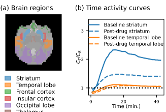
A numerical phantom was used to quantitatively evaluate the proposed method. The numerical phantom was constructed from the non-human primate (NHP) NIH macaque template (NMT) [45, 46], which was used to generate a brain atlas for PET comprised of 13 regions. Kinetic parameters were assigned to each region of the phantom based on SRTM analysis of in-vivo NHP [¹¹C]MK-6884 PET scans. Noiseless dynamic PET images were then synthesized with the SRTM model using the gray matter cerebellum as reference region [32]. To mimic an occupancy study, changes in $\mathrm{BP}_{ND}$ were introduced between the baseline and post-drug scan, corresponding to a receptor occupancy $\mathrm{RO}$ following the Hill model in (6). Two simulations were used: one where the $\mathrm{RO}$ map was chosen to be uniform across brain regions and one where the $\mathrm{RO}$ map varies in a brain region. Brain regions of the atlas as well as representative time activity curves are shown in Fig. 1.

Dynamic PET projections were then obtained by forward-projecting the noise-free dynamic images mimicking the geometry of a Discovery MI PET/CT scanner (GE Healthcare). Poisson deviates were applied to the obtained PET sinograms to approach the noise level in a typical in-vivo NHP scan.

The proposed method was evaluated via bias-variance analysis. The proposed joint direct parametric reconstruction (‘JDPR’) was compared to standard indirect methods: indirect parametric reconstruction (‘IPR’) consisting in OSEM reconstruction of dynamic PET images followed by SRTM fitting using basis functions [38] and OSEM reconstruction of dynamic PET images with post-reconstruction Gaussian smoothing followed by SRTM fitting (‘IPRs’). Additionally the proposed method was compared to a method representative of existing direct parametric reconstruction methods (‘DPR’), i.e., replacing the joint penalty on receptor occupancy ($\beta_{RO}=0$ in (11)) by Bowsher regularization of post-drug binding potential. DPR was applied to each scan separately, before estimating RO. For this analysis, pixel-wise bias and standard deviation were calculated using:

$$\mathrm{bias} =\frac{1}{K}\sum_{k=1}^{K}\theta^{(k)}-\hat{\theta}$$ (20)

$$\mathrm{std} =\frac{1}{K-1}\sum_{k=1}^{K}(\theta^{(k)}-\bar{\theta})^{2},$$ (21)

where $K$ is the number of noise realizations, $\theta^{(k)}$ is a set of reconstructed kinetic parameter maps for noise realization $k$, $\hat{\theta}$ is the set of ground truth kinetic parameter maps and $\bar{\theta}=\frac{1}{K}\sum_{k=1}^{K}\theta^{(k)}$. In order to avoid extreme, physiologically implausible values for estimated kinetic parameters that may severely impact bias and variance estimates, reconstructed kinetic parameter maps were first clipped. Bias-variance curves were obtained for each method by varying reconstruction parameters: for IPR, the reconstruction parameter was the number of iterations; for IPRs, the Gaussian filter full width at half maximum (FWHM); for DPR, the regularizer strength $\beta_{BP}$ was varied to obtain the curve; finally, for the proposed method (JDPR), the regularizer strength $\beta_{BP}$ and $\beta_{RO}$ were used to obtain the bias-variance curve.

II-E In-vivo studies

The proposed method was applied to data acquired in two non-human primates (with weights ranging from 12.2 kg to 13.4 kg and from 15.1 kg to 17.7 kg across studies) using [¹¹C]MK-6884, a muscarinic acetylcholine receptor 4 (M4) ligand and CVL-231, an M4 positive allosteric modulator under development. All acquisitions were performed on a GE PET/CT Discovery MI scanner. The study protocol, described in detail in [9], included two dynamic PET scans: one at baseline and the other under a blocking condition with intravenous administration of CVL-231 by bolus-plus-infusion (loading dose of 0.8 mg/kg given 10 min before radiotracer followed by constant infusion of varying concentration–0.25, 0.5, 1, 1.7 and 3.4 mg/kg–for a 90 minute administration protocol). Dynamic studies were truncated to 45 minutes. In total, 7 pairs of scans were performed at different CVL-231 concentrations. Baseline and post-drug studies were performed with the same field of view and subject position, therefore registration between scans was not required. In the absence of ground truth, the proposed method was compared in terms of agreement with baseline methods in the striatum, a region with a higher M4 receptor density and therefore higher signal-to-noise ratio.

III Results

Fig. 2: Bias/standard deviation plots for baseline $\mathrm{BP}_{ND}$ estimation averaged in the striatum (top) and temporal lobe (bottom) regions. Each plot was obtained by varying a reconstruction parameter for each method (varying the iteration number for IPR, the post-reconstruction Gaussian filter width for IPRs, $\beta_{BP}$ for DPR and JDPR). The vertical orange dashed line indicates the reference reconstruction setting for the IPRs method (1.5 mm FWHM filter) used for the bias/standard deviation maps shown in Fig. 3. The star markers for each method indicate the selected parameter best approaching the reference reconstruction setting in the striatum.

Fig. 3: Bias (top) and standard deviation (bottom) maps for $\mathrm{BP}_{ND}$ estimation for the different methods. Reconstruction settings for each method are indicated by stars in Fig. 2.

Fig. 4: Bias/standard deviation plots for RO estimation averaged in, from left to right, the striatum, insular cortex, temporal lobe and whole brain. The true parameter value is indicated in the title. Each plot was obtained by varying a reconstruction parameter for each method (varying the iteration number for IPR, the post-reconstruction Gaussian filter width for IPRs, $\beta_{BP}$ for DPR and $\beta_{RO}$ for JDPR). The vertical orange dashed line indicates the reference reconstruction setting for the IPRs method (4 mm FWHM filter). The star markers, for each method the selected parameter best approaching the reference reconstruction setting in the striatum.

Fig. 5: Bias (top) and standard deviation (bottom) maps for RO estimation for different reconstruction methods with settings indicated by stars in Fig. 4.

Fig. 6: Baseline binding potential (top) and receptor occupancy maps for a single noise realization and settings indicated by stars in Fig. 4. Values are clipped to the intensity range displayed in the color bar (pixels with out-of-range low values are in black, high values are in dark red).

Fig. 7: Binding potential (top) and receptor occupancy maps for a single noise realization with spatially varying receptor occupancy, and settings indicated by stars in Fig. S.3.2. Values are clipped to the intensity range displayed in the color bar (pixels with out-of-range low values are in black, high values are in dark red).

Fig. 8: Estimated receptor occupancy for each method (crosses) as a function of simulated drug concentration compared to ground truth Hill curve used for the simulation. The shaded region shows the 20%-80% percentiles of the fitted Hill curve over 50 noise realizations, in each region, excluding outliers. The proposed method best approaches the ground-truth curve, especially in low binding regions. Note that the envelope region is omitted for IPR, IPRs and DPR outside of the striatum, where these methods yield unreliable RO estimates.

III-A Simulation phantom

The phantom described in Section II-D was used to compare the different reconstruction methods. For this evaluation, the receptor occupancy was fixed to 66% (following (6) with $E_{max}=1$, $\frac{ED_{50}}{c}=\frac{1}{2}$) in the whole brain and 50 noise realizations were reconstructed. The proposed joint direct method was compared to conventional parametric estimation: (1) IPR with 12 OSEM subsets, varying the number of iterations, (2) IPRs with a fixed number of iterations and subsets varying Gaussian filter FWHMs and (3) DPR varying $\beta_{\mathrm{BP}_{ND}}$. Both the direct and proposed joint-direct methods used a Huber spatial prior [47]. Methods were compared in the striatum (a high-binding region for this particular tracer), the temporal lobe (a low binding region) and the whole brain.

Fig. 9: Kinetic parameter images for the NHP [¹¹C]MK-6884 occupancy study at different drug concentrations. For each concentration, the baseline, post-drug BP (overlaid on the MR image), and the RO map are shown for each method: (top) IPR, (middle row) IPRs with 4 mm Gaussian filter and (bottom) proposed JDPR method. For all concentrations, the proposed method results in improved RO estimates, especially in low binding regions.

The bias/standard deviation plots for baseline $\mathrm{BP}_{ND}$ estimation are shown in Fig. 2. The curves were obtained by varying reconstruction parameters controlling the bias/standard deviation trade-off, i.e., varying the iteration number for IPR (from 1 to 9 iterations), the post-reconstruction Gaussian filter width for IPRs (from 1 to 7 mm), $\beta_{BP}$ for DPR and JDPR (from $\beta_{BP}=1$ to $\beta_{BP}=500$). The curves demonstrate the improvement of both DPR and proposed JDPR over indirect estimation methods. As expected, in the striatum as well as in low binding regions, the proposed and direct methods both achieved consistently low bias, as well as lower standard deviation at a given bias level than the conventional methods. The proposed method, as well as direct reconstruction, were able to match this low bias while reducing standard deviation three-fold compared to the reference reconstruction indicated by the vertical orange dotted line. In this study, the reference reconstruction setting was selected arbitrarily to result in low bias in the striatum, using a Gaussian filter with FWHM 1.5 mm. Bias and variance maps shown on Fig. 3 illustrate the dramatic improvement both in bias and standard deviation as compared to conventional indirect methods.

Fig. 4 presents bias and standard deviation plots of $\mathrm{RO}$ estimates when varying reconstruction parameters for each method. The curves were obtained by varying reconstruction parameters controlling the bias/standard deviation trade-off, i.e., varying the iteration number for IPR, the post-reconstruction Gaussian filter width for IPRs, $\beta_{BP}$ (from $\beta_{BP}=1$ to $\beta_{BP}=100$) for DPR and $\beta_{\mathrm{RO}}$ (from $\beta_{\mathrm{RO}}=500$ to $\beta_{\mathrm{RO}}=10000$) for JDPR. In the striatum, the proposed method approached the performance of the conventional approach used to estimate receptor occupancy, i.e. OSEM reconstruction followed by Gaussian filtering (FWHM = 4 mm) and SRTM fitting (indicated by the vertical orange dashed line in the figure). The proposed method offered a reduction in standard deviation for equal bias for $\mathrm{RO}$ estimates compared to the conventional methods (40% reduction over IPRs for the operating points marked by a star). Direct reconstruction likewise achieved a low bias and low standard deviation in the striatum. The improvement afforded by JDPR was much more pronounced in brain regions with intermediate to lower receptor densities, where IPR, IPRs and DPR methods introduced a large bias (over 20% for indirect methods) with high variance, whereas the proposed method resulted in low bias and variance, consistent with results obtained in the striatum. Corresponding bias and variance maps for the reconstruction settings marked by a star in Fig. 4 are shown in Fig. 5, while Fig. 6 presents representative examples of $\mathrm{BP}_{ND}$ and RO images for a single noise realization. They confirm the improvement offered by the proposed method, which matched the low bias observed in the reference reconstruction (IPRs) while dramatically reducing the bias in other regions. A similar reduction was observed on the standard deviation map, confirming that the proposed method can yield more accurate and robust estimates. Figure 6 also shows improved $\mathrm{BP}_{ND}$ estimation for the DPR and JDPR methods. This is a result of the direct estimation approach, which improves the precision of $\mathrm{BP}_{ND}$ estimates. An example of ADMM cost evolution over iterations is shown in Supplemental Material Fig. S.2.

The proposed method penalizes variance in the receptor occupancy map, based on the commonly used assumption that blocking drug effects are mostly uniform across the brain. In order to evaluate the performance of the proposed algorithm when this assumption is not valid, a numerical simulation was carried out with a nonuniform receptor occupancy map, set at 60% in striatum and 50% in the rest of the brain.

Representative results for a single noise realization shown in Fig. 7 demonstrate the ability of JDPR to capture spatial variations in receptor occupancy. Bias-variance analysis reported in Supplemental Material (Figs. S.3.2 and S.3.1) shows that the proposed method achieved a similar level of bias and variance as for the uniform RO case.

Finally, numerical simulations were performed for different drug concentration–and thus occupancy–levels. The simulated receptor occupancy followed the Hill equation in (6). Fifty noise realizations were simulated for each concentration level. RO values were averaged in each region for each method, and for each noise realization, the Hill equation was fitted to the regional RO estimates plotted as function of the simulated concentration level. The receptor occupancy values estimated by each method are shown, along with the Hill curve fits, in Fig. 8. The shaded curve envelopes correspond to the 20%-80% percentiles across noise realizations. A summary of the RO estimation performance, measured in term of bias and standard deviation is reported in Supplemental Material Table S.5. In the striatum, all methods resulted in good RO estimation, the proposed method yielding the lowest variance, at the expense of a slight loss of accuracy (around 5%). In other regions, typically with lower binding and thus SNR, conventional methods failed to capture the shape of the Hill curve owing to large errors in RO estimation (the confidence intervals in Fig. 8 were omitted for the IPR, IPRs and DPR in non-striatal regions since the fitted RO values are severely biased, preventing direct comparison with JDPR). By contrast, the proposed method consistently estimated RO for all concentrations with high accuracy and low variance, with a slight error increase for high receptor occupancy in low binding regions. This is confirmed by the high R-squared values ($>$ 90%) reported in Supplemental Material Table S.5.

III-B In-vivo experiments

Fig. 10: Estimated RO values and fitted Hill curve for in-vivo data in different brain regions. Dashed vertical lines indicate the estimated $ED_{50}$. While all methods result in estimated RO values in agreement with the logistic Hill curve in the striatum, only the proposed method achieves a similar performance in other brain regions.

The proposed method was evaluated on the in-vivo data described in Section II-E. Representative kinetic parameter maps are shown in Fig. 9. In this study, $\beta_{BP}$ was selected such that the proposed joint direct reconstruction matches the bias level of the $\mathrm{BP}_{ND}$ parameter achieved by the conventional indirect method in the striatum. $\beta_{RO}$ was selected to match the RO bias of the conventional indirect method in the striatum. The proposed method resulted in improved RO estimation, especially in low binding regions. The estimation of baseline $\mathrm{BP}_{ND}$ was also improved, achieving a contrast recovery in the striatum similar to the IPR method with a reduced noise level. The reduction in variance also translated into improved fitting of the Hill curve (6) (Fig. 10). While no ground truth RO was available for in-vivo data, the proposed method resulted in RO estimates matching with the logistic curve, suggesting that the estimated values are consistent with the model. Additionally, the $ED_{50}$ estimate for JDPR in all brain regions was consistent with that obtained in the striatum, enabling estimation of RO from the whole brain, which, we hypothesize, will give more power to receptor occupancy studies.

IV Discussions

The proposed joint-direct reconstruction framework relies on the minimization of an objective function linking PET projection measurements to kinetic parameter maps and including a joint prior on the baseline and post-drug scans. This formulation achieves two objectives: (1) bias control in estimation of kinetic parameters thanks to the log-likelihood term and (2) application of a variance penalty on receptor occupancy distribution (resulting from the assumption of uniform drug exposure in the brain). This enables accurate and precise estimation of RO in regions with lower receptor density from all the brain regions. From Fig. 4, it is worth noting that, in the striatum, both IPRs and DPR could achieve ideal RO estimation with near zero bias and standard deviation. This is a consequence of the RO calculation where biases in $\mathrm{BP}_{ND}$ estimates from baseline and post-drug scans cancel each other (which explains the shape of the curve where reduction in variance is accompanied by reduction in bias, contrary to the more usual trend seen, e.g. in Fig. 2). In this work, the parameter for IPRs used as reference was selected to achieve a reasonable balance between RO and BP bias.

Since the variance penalty is implemented as a soft constraint, the proposed method can relax the hypothesis of uniform receptor occupancy [25] as shown in Fig. 7 and Supplemental Material Figs. S.3.2 and S.3.1. Therefore, the proposed method is able to exploit RO uniformity when relevant but still provide the benefits of direct parametric mapping and joint RO estimation when the uniform RO constraint is relaxed. This could happen, for instance, in cases where the radiotracer binds to more targets than the drug under investigation.

While the reported evaluations performed on simulations and in-vivo data did not include motion in the measurements, incorporation of rigid motion is straightforward in the proposed estimation framework. It only requires the addition of a rigid deformation operator in the forward model (2), resulting in increased computational cost, but otherwise no change to the estimation framework, which, we expect, will enable scanning over multiple days, without need for sedation.

One limitation of the evaluation is the tracer used for the study. [¹¹C]MK-6884 is characterized by high binding in the striatum, low binding in most other regions of the brain and few regions with intermediate level of binding. In future work, the proposed method will be applied to other tracers and drug candidates to evaluate its performance with different tracer distributions. The simulation results give an indication of the performance of proposed method in regions with intermediate levels of binding. As shown in Fig. 4, the insular cortex region was assigned an intermediate $\mathrm{BP}_{ND}$ value ($BP=0.315$), and bias/standard deviation curves show the improvement offered by JDPR over conventional methods. The proposed method may offer diminishing benefits for tracers with high binding in the whole brain. In this case, the method may still be beneficial for low count data.

Another limitation is the number of hyperparamaters to select, namely the regularization strengths and ADMM auxiliary variables. In practice, the regularization parameters are coupled based on the expected dynamic ranges as described in Section II-C and selected by targetting a fixed ratio between log-likelihood and regularization. ADMM parameters ($\rho$ and $\mu$) are selected from a single iteration to minimize the cost of the corresponding subproblems.

V Conclusion

This paper proposes a joint direct reconstruction for receptor occupancy estimation from baseline and post-drug PET scans. The proposed method combines direct parametric estimation with a prior on the receptor occupancy map estimated from both scans. Validation on numerical simulations demonstrated improved the bias variance trade-off compared to traditional indirect as well as non-joint direct methods, especially in regions with low receptor densities which are often excluded from occupancy analyses due to the poor estimation performance. The proposed method was successfully applied to in-vivo MK-6884 data to characterize the relationship between drug concentration and receptor occupancy. The reduction in estimation variance achieved with the proposed method could be used to reduce the sample size required for occupancy studies and/or decrease radiation exposure in study subjects for tracers with low and intermediate binding regions.

Supplemental material

S.1 Penalized kinetic fitting using basis functions

This section describes the method used to minimize (18). The problem is reformulated into the following generic form:

$$\gamma^{*}=\arg\min_{\gamma}\frac{\rho}{2}\left\|z-C(\gamma)\right\|_{W}^{2}+\frac{\mu}{2}\left\|\zeta-h(\gamma)\right\|_{\Lambda}^{2},$$ (S.1.1)

where $z$ is the concatenation of the dynamic PET images for baseline and post-drug scans and $\zeta$ is the set of kinetic parameters: $\zeta=[\zeta_{\mathrm{BP}_{ND}^{(B)}},\zeta_{k_{2}^{(B)}},\zeta_{R_{1}^{(B)}},\zeta_{\mathrm{BP}_{ND}^{(D)}},\zeta_{k_{2}^{(D)}},\zeta_{R_{1}^{(D)}}]$.

The problem in (S.1.1) is modified to enable the use of the basis function technique described in [38]. The strategy consists in extracting the nonlinear components of the operators in quadratic terms into basis functions and express the overall optimization problem as a sum of quadratic terms with linear operators for each basis function. The kinetic operator $C(\gamma)$ can be reformulated as in [38], taking into a account the two scans, resulting in:

$$C(\gamma) = \left[\begin{matrix}E_{\kappa^{(B)}}&F_{\kappa^{(B)}}&0&0\\ 0&0&E_{\kappa^{(D)}}&F_{\kappa^{(D)}}\end{matrix}\right]\,$$ [ k 2 (B) R 1 (B) k 2 (D) R 1 (D) ] (S.1.2)

$$\triangleq \mathcal{C}_{\kappa}\,$$ ~ γ ,

where $\tilde{\gamma}=[k_{2}^{(B)},R_{1}^{(B)},k_{2}^{(D)},R_{1}^{(D)}]$ and the basis functions are expressed as $E_{\kappa}=C_{R}(t)\ast\exp\left(-\kappa t\right)$ and $F_{\kappa}=C_{R}-\kappa\,E_{\kappa}$ with $\kappa=\frac{k_{2}}{1+\mathrm{BP}_{ND}}$. Basis functions are precalculated for pairs of $\kappa=(\kappa^{(B)},\kappa^{(D)})$ values.

The second quadratic term can be reformulated as:

$$\zeta-h(\gamma) = \left[\begin{matrix}\zeta_{\mathrm{BP}_{ND}^{(B)}}+1\\ \zeta_{k_{2}^{(B)}}\\ \zeta_{R_{1}^{(B)}}\\ \zeta_{\mathrm{BP}_{ND}^{(D)}}+1\\ \zeta_{k_{2}^{(D)}}\\ \zeta_{R_{1}^{(D)}}\end{matrix}\right]$$ - [ 1 κ (B) 0 0 0 1 0 0 0 0 1 0 0 0 0 1 κ (D) 0 0 0 1 0 0 0 0 1 ] [ k 2 (B) R 1 (B) k 2 (D) R 1 (D) ] (S.1.3)

$$\triangleq \tilde{\zeta}$$ - H_κ ~ γ ,

where we used $\mathrm{BP}_{ND}=\frac{k_{2}}{\kappa}-1$.

The transformed objective function is:

$$\tilde{\gamma}_{\kappa}^{*}=\arg\min_{\gamma}\frac{\rho}{2}\left\|z-\mathcal{C}_{\kappa}\,\tilde{\gamma}\right\|_{W}^{2}+\frac{\mu}{2}\left\|\tilde{\zeta}-H_{\kappa}\,\tilde{\gamma}\right\|_{\Lambda}^{2},$$ (S.1.4)

which can now be solved analytically:

$$\tilde{\gamma}_{\kappa}^{*}=\left(\rho C_{\kappa}^{\top}WC_{\kappa}+\mu H_{\kappa}^{\top}\Lambda H_{\kappa}\right)^{-1}\left(\rho C_{\kappa}^{\top}Wz+\mu H_{\kappa}^{\top}\Lambda\tilde{\zeta}\right).$$ (S.1.5)

After calculating $\tilde{\gamma}_{\kappa}^{*}$ for a grid of $(\kappa^{(B)},\kappa^{(D)})$ pairs, the final step of the optimization procedure consists in finding the pair resulting in the smallest cost in (S.1.4) and use the corresponding $\tilde{\gamma}_{\kappa}^{*}$ to assign the $k_{2}$ and $R_{1}$ kinetic parameters, thus solving (S.1.1).

S.2 ADMM convergence

Fig. S.2: ADMM cost as function of iterations for single noise realization with parameters used in Fig. 6. Parametric maps ($\mathrm{BP}_{ND}$ and RO) are shown for the initial estimate and final iteration.

S.3 Simulation with varying receptor occupancy

This section reports the results of the numerical simulation performed assuming a spatially varying receptor occupancy. Figure S.3.1 shows bias and standard deviation maps for different methods and Fig. S.3.2 shows the bias/standard deviation plots for varying reconstruction parameters.

Fig. S.3.1: Bias/standard deviation maps for images indicated by stars in Fig S.3.2.

Fig. S.3.2: Bias/standard deviation plots for RO estimation averaged in the striatum (left), temporal lobe (middle) and whole brain (right) regions for the base of a nonuniform RO distribution (RO = 0.6 in the striatum and 0.5 in the rest of the brain). The vertical orange dashed line indicates the reference reconstruction setting for the IPRs method (4 mm FWHM filter). The star markers, for each method the selected parameter best approaching the reference reconstruction setting.

S.4 Reconstruction parameters

TABLE S.4: Reconstruction parameters for JDPR method: for simulations, parameters used to obtain results indicated by a star in Fig. 4; for in-vivo reconstruction: parameters used to obtain results in Fig. 9 (1 mg/kg).

Parameter	Simulation	In-vivo
$\beta_{0}$	10	0.01
$\beta_{RO}$	1000	1
$\rho$	5	1
$\mu$	100	1
Outer ADMM iterations (Eqs. 13, 14, 15)	15	8
Inner ADMM iterations (Eqs. 17, 18, 19)	6	6
CG iterations (Eq. 17)	4	4
BSREM iterations	4	4
BSREM subsets	12	12

S.5 Bias variance of RO estimates over concentration (simulation)

TABLE S.5: Bias/standard deviation of RO estimates in Hill curve in Fig. 8 for different regions. Each cell shows the bias / standard deviation in percent of the true RO value. The last columns reports the R-squared of the fit, averaged over noise realizations.

Region	Method	Concentration (mg/mL)					R-squared
		10.0 (RO=2%)	100.0 (RO=16.7%)	1000.0 (RO=66.7%)	10000.0 (RO=95.2%)	100000.0 (RO=99.5%)
Striatum	IPR	65.5 / 362.0	20.0 / 38.9	-0.1 / 5.8	-0.4 / 4.9	-0.6 / 4.7	0.981
	IPRs	2.5 / 383.8	12.4 / 36.0	0.1 / 9.3	-0.6 / 9.9	0.1 / 6.8	0.963
	DPR	-114.3 / 242.7	-4.3 / 23.7	-0.7 / 4.9	-0.7 / 3.8	-1.4 / 3.2	0.993
	JDPR	-85.4 / 343.8	-1.4 / 33.6	-5.8 / 7.9	-5.1 / 6.8	-5.5 / 6.4	0.972
Temporal lobe	IPR	3303.0 / 523.8	298.7 / 61.5	-0.4 / 14.1	-28.6 / 11.0	-33.3 / 8.3	-32.952
	IPRs	1118.6 / 1142.9	80.4 / 104.1	-42.0 / 31.6	-63.4 / 19.1	-57.6 / 21.3	-3.524
	DPR	2046.3 / 707.6	186.6 / 87.5	-26.5 / 23.9	-42.1 / 15.9	-44.7 / 16.6	-9.668
	JDPR	-150.7 / 447.7	-7.8 / 49.1	-12.4 / 12.7	-12.4 / 12.2	-11.8 / 9.3	0.901
Whole brain	IPR	2575.5 / 206.9	233.0 / 24.6	-4.4 / 4.9	-29.7 / 3.8	-32.1 / 3.4	-24.525
	IPRs	715.2 / 662.2	31.3 / 69.3	-36.2 / 16.5	-46.9 / 11.9	-45.7 / 11.4	-1.872
	DPR	1817.4 / 556.3	156.6 / 76.7	-23.2 / 21.6	-38.3 / 14.3	-37.7 / 13.2	-7.678
	JDPR	-146.1 / 434.8	-7.4 / 47.5	-11.7 / 12.4	-11.9 / 11.5	-11.2 / 9.0	0.91

References

- [1] J. A. DiMasi, R. W. Hansen, and H. G. Grabowski, “The price of innovation: new estimates of drug development costs,” Journal of Health Economics, vol. 22, no. 2, pp. 151–185, 2003.
- [2] D. F. Wong, J. Tauscher, and G. Grunder, “The role of imaging in proof of concept for CNS drug discovery and development,” Neuropsychopharmacology, vol. 34, no. 1, pp. 187–203, 2009.
- [3] C.-M. Lee and L. Farde, “Using positron emission tomography to facilitate CNS drug development,” Trends in Pharmacological Sciences, vol. 27, no. 6, pp. 310–316, 2006.
- [4] J. Khodaii et al., “Relative Strengths of Three Linearizations of Receptor Availability: Saturation, Inhibition, and Occupancy Plots,” Journal of Nuclear Medicine, vol. 63, no. 2, pp. 294–301, 2022.
- [5] V. J. Cunningham et al., “Measuring drug occupancy in the absence of a reference region: the Lassen plot re-visited,” Journal of Cerebral Blood Flow and Metabolism, vol. 30, no. 1, pp. 46–50, 2010.
- [6] N. A. Lassen et al., “Benzodiazepine receptor quantification in vivo in humans using [11C]flumazenil and PET: application of the steady-state principle,” Journal of Cerebral Blood Flow and Metabolism, vol. 15, no. 1, pp. 152–165, 1995.
- [7] M. Naganawa et al., “Receptor Occupancy of the kappa-Opioid Antagonist LY2456302 Measured with Positron Emission Tomography and the Novel Radiotracer 11C-LY2795050,” The Journal of Pharmacology and Experimental Therapeutics, vol. 356, no. 2, pp. 260–266, 2016.
- [8] M. Naganawa et al., “Quantitative PET Imaging in Drug Development: Estimation of Target Occupancy,” Bulletin of Mathematical Biology, vol. 81, no. 9, pp. 3508–3541, 2019.
- [9] V. Belov et al., “PET imaging of M4 muscarinic acetylcholine receptors in rhesus macaques using [11C]MK-6884: Quantification with kinetic modeling and receptor occupancy by CVL-231 (emraclidine), a novel positive allosteric modulator,” Journal of Cerebral Flow and Metabolism, vol. 44, no. 8, pp. 1329–1342, 2024.
- [10] F. A. Kotasidis, C. Tsoumpas, and A. Rahmim, “Advanced kinetic modelling strategies: towards adoption in clinical PET imaging,” Clinical and Translational Imaging, vol. 2, no. 3, pp. 219–237, 2014.
- [11] G. I. Angelis et al., “Convergence optimization of parametric MLEM reconstruction for estimation of Patlak plot parameters,” Computerized Medical Imaging and Graphics, vol. 35, no. 5, pp. 407–416, 2011.
- [12] M. E. Kamasak et al., “Direct reconstruction of kinetic parameter images from dynamic PET data,” IEEE Transactions on Medical Imaging, vol. 24, no. 5, pp. 636–650, 2005.
- [13] G. Wang and J. Qi, “Acceleration of the direct reconstruction of linear parametric images using nested algorithms,” Physics in Medicine and Biology, vol. 55, no. 5, pp. 1505–1517, 2010.
- [14] G. Wang and J. Qi, “An optimization transfer algorithm for nonlinear parametric image reconstruction from dynamic PET data,” IEEE Transactions on Medical Imaging, vol. 31, no. 10, pp. 1977–1988, 2012.
- [15] G. Wang and J. Qi, “Direct estimation of kinetic parametric images for dynamic PET,” Theranostics, vol. 3, no. 10, pp. 802–815, 2013.
- [16] N. A. Karakatsanis et al., “Whole-body direct 4D parametric PET imaging employing nested generalized Patlak expectation-maximization reconstruction,” Physics in Medicine and Biology, vol. 61, no. 15, pp. 5456–5485, 2016.
- [17] J. Jiao et al., “Direct Parametric Reconstruction With Joint Motion Estimation/Correction for Dynamic Brain PET Data,” IEEE Transactions on Medical Imaging, vol. 36, no. 1, pp. 203–213, 2017.
- [18] K. Gong et al., “Direct Patlak Reconstruction From Dynamic PET Data Using the Kernel Method With MRI Information Based on Structural Similarity,” IEEE Transactions on Medical Imaging, vol. 37, no. 4, pp. 955–965, 2018.
- [19] R. Loeb, N. Navab, and S. I. Ziegler, “Direct Parametric Reconstruction Using Anatomical Regularization for Simultaneous PET/MRI Data,” IEEE Transactions on Medical Imaging, vol. 34, no. 11, pp. 2233–2247, 2015.
- [20] Y. Rakvongthai et al., “Direct reconstruction of cardiac PET kinetic parametric images using a preconditioned conjugate gradient approach,” Medical Physics, vol. 40, no. 10, p. 102501, 2013.
- [21] Y. Petibon et al., “Direct parametric reconstruction in dynamic PET myocardial perfusion imaging: in vivo studies,” Physics in Medicine and Biology, vol. 62, no. 9, pp. 3539–3565, 2017.
- [22] Y. Petibon et al., “PET imaging of neurotransmission using direct parametric reconstruction,” NeuroImage, vol. 221, p. 117154, 2020.
- [23] K. Gong et al., “Nonlinear PET parametric image reconstruction with MRI information using kernel method,” in SPIE Medical Imaging, vol. 101321G, 2017.
- [24] S. Boyd et al., “Distributed Optimization and Statistical Learning via the Alternating Direction Method of Multipliers,” Foundations and Trends in Machine Learning, vol. 3, no. 1, pp. 1–122, 2011.
- [25] B. de Laat and E. D. Morris, “A local-neighborhood Lassen plot filter for creating occupancy and non-displaceable binding images,” Journal of Cerebral Blood Flow and Metabolism, vol. 41, no. 6, pp. 1379–1389, 2021.
- [26] K. Vunckx et al., “Evaluation of three MRI-based anatomical priors for quantitative PET brain imaging,” IEEE Transactions on Medical Imaging, vol. 31, no. 3, pp. 599–612, 2012.
- [27] T. Marin et al., “Joint direct parametric reconstruction for PET receptor occupancy mapping,” in IEEE Nuclear Science Symposium, 2020.
- [28] T. Marin et al., “PET mapping of receptor occupancy using joint direct parametric reconstruction: in-vivo studies,” in Society of Nuclear Medicine & Molecular Imaging Conference, vol. 63, no. supplement 2, 2022.
- [29] S. Ellis and A. J. Reader, “Simultaneous maximum a posteriori longitudinal PET image reconstruction,” Physics in Medicine and Biology, vol. 62, no. 17, pp. 6963–6979, 2017.
- [30] S. Ellis and A. J. Reader, “Penalized maximum likelihood simultaneous longitudinal PET image reconstruction with difference-image priors,” Medical Physics, vol. 45, no. 7, pp. 3001–3018, 2018.
- [31] S. Duvvuri et al., “Evaluation of M4 Muscarinic Receptor Occupancy by CVL-231 Using [11C] MK-6884 PET in Nonhuman Primates,” Neuropsychopharmacology, vol. 46, no. 1, p. 342, 2021.
- [32] W. Li et al., “The PET tracer [(11)C]MK-6884 quantifies M4 muscarinic receptor in rhesus monkeys and patients with Alzheimer’s disease,” Science Translational Medicine, vol. 14, no. 627, p. eabg3684, 2022.
- [33] H. M. Hudson and R. S. Larkin, “Accelerated image reconstruction using ordered subsets of projection data,” IEEE Transactions on Medical Imaging, vol. 13, no. 4, pp. 601–609, 1994.
- [34] S. Ahn and J. A. Fessler, “Globally convergent image reconstruction for emission tomography using relaxed ordered subsets algorithms,” IEEE Transactions on Medical Imaging, vol. 22, no. 5, pp. 613–626, 2003.
- [35] R. N. Gunn, S. R. Gunn, and V. J. Cunningham, “Positron emission tomography compartmental models,” Journal of Cerebral Blood Flow and Metabolism, vol. 21, no. 6, pp. 635–652, 2001.
- [36] A. A. Lammertsma and S. P. Hume, “Simplified reference tissue model for PET receptor studies,” NeuroImage, vol. 4, no. 3 Pt 1, pp. 153–158, 1996.
- [37] R. B. Innis et al., “Consensus nomenclature for in vivo imaging of reversibly binding radioligands,” Journal of Cerebral Blood Flow and Metabolism, vol. 27, no. 9, pp. 1533–1539, 2007.
- [38] R. N. Gunn et al., “Parametric imaging of ligand-receptor binding in PET using a simplified reference region model,” NeuroImage, vol. 6, no. 4, pp. 279–287, 1997.
- [39] M. Yaqub et al., “Optimization algorithms and weighting factors for analysis of dynamic PET studies,” Physics in Medicine and Biology, vol. 51, no. 17, pp. 4217–4232, 2006.
- [40] J. MacDougall, Analysis of Dose–Response Studies-Emax Model. New York, NY: Springer New York, 2006, pp. 127–145.
- [41] M. Defrise et al., “Exact and approximate rebinning algorithms for 3-D PET data,” IEEE Transactions on Medical Imaging, vol. 16, no. 2, pp. 145–158, 1997.
- [42] R. L. Siddon, “Fast calculation of the exact radiological path for a three-dimensional CT array,” Medical Physics, vol. 12, no. 2, pp. 252–255, 1985.
- [43] F. Jacobs et al., “A Fast Algorithm to Calculate the Exact Radiological Path through a Pixel or Voxel Space,” Journal of Computing and Information Technology, vol. 6, no. 1, pp. 89–94, 1998.
- [44] M. Germino and R. E. Carson, “Cardiac-gated parametric images from (82) Rb PET from dynamic frames and direct 4D reconstruction,” Medical Physics, vol. 45, no. 2, pp. 639–654, 2018.
- [45] B. Jung et al., “A comprehensive macaque fMRI pipeline and hierarchical atlas,” NeuroImage, vol. 235, p. 117997, 2021.
- [46] J. Seidlitz et al., “A population MRI brain template and analysis tools for the macaque,” NeuroImage, vol. 170, pp. 121–131, 2018.
- [47] D. F. Yu and J. A. Fessler, “Edge-preserving tomographic reconstruction with nonlocal regularization,” IEEE Transactions on Medical Imaging, vol. 21, no. 2, pp. 159–173, 2002.