AutoFLUKA: A Large Language Model Based Framework for Automating Monte Carlo Simulations in FLUKA
Abstract
Monte Carlo (MC) simulations, particularly using FLUKA, are essential for replicating real-world scenarios across scientific and engineering fields. Despite the robustness and versatility, FLUKA faces significant limitations in automation and integration with external post-processing tools, leading to workflows with a steep learning curve, which are time-consuming and prone to human errors. Traditional methods involving the use of shell and Python scripts, MATLAB, and Microsoft Excel require extensive manual intervention and lack flexibility, adding complexity to evolving scenarios. This study explores the potential of Large Language Models (LLMs) and AI agents to address these limitations. AI agents, integrate natural language processing with autonomous reasoning for decision-making and adaptive planning, making them ideal for automation. We introduce AutoFLUKA, an AI agent application developed using the LangChain Python Framework to automate typical MC simulation workflows in FLUKA. AutoFLUKA can modify FLUKA input files, execute simulations, and efficiently process results for visualization, significantly reducing human labor and error. Our case studies demonstrate that AutoFLUKA can handle both generalized and domain-specific cases, such as Microdosimetry, with an streamlined automated workflow, showcasing its scalability and flexibility. The study also highlights the potential of Retrieval Augmentation Generation (RAG) tools to act as virtual assistants for FLUKA, further improving user experience, time and efficiency. In conclusion, AutoFLUKA represents a significant advancement in automating MC simulation workflows, offering a robust solution to the inherent limitations. This innovation not only saves time and resources but also opens new paradigms for research and development in high energy physics, medical physics, nuclear engineering space and environmental science.
keywords:
Monte Carlo Simulations , FLUKA Automation , Large Language Models , AI Agents , Retrieval Augmented Generation[label1]organization=Department of Nuclear Engineering, Texas A&M University,country=United States
[label2]organization=College of Performance, Visualization & Fine Arts, Texas A&M University, country=United States
AutoFLUKA is an AI-driven tool that automates complex Monte Carlo simulation workflows, integrating seamlessly with FLUKA.
It reduces human intervention and minimizes errors by automating input generation, simulation execution, and post-processing.
AutoFLUKA introduces JSON-based data outputs, enabling easier downstream analysis compared to traditional manual approaches.
AutoFLUKA includes a Retrieval Augmented Generation tool that serves as a virtual assistant, helping users address common FLUKA challenges by providing quick, context-specific guidance.
1 Introduction
Monte Carlo (MC) simulations are virtual experiments that replicate real-world scenarios using statistical methods. These simulations are crucial for accurately modeling complex physical processes, such as radiation transport and particle interactions with matter that could be otherwise expensive, time consuming or resource-intensive. Particularly, FLUKA (FLUktuierende Kaskade) is a versatile MC simulation package with proven applicability across various fields of science and engineering. Originally developed at the European Organization for Nuclear Research (CERN) in the 1960s, then later, jointly by CERN and the Italian National Institute of Nuclear Physics (INFN), FLUKA has evolved into a multi-purpose tool capable of simulating the interaction and transport of over 60 different particles across a wide range of energies in matter (Ahdida et al., 2022; Böhlen et al., 2014; Fassò et al., 2012)
FLUKA simulations have been extensively used to advance research and innovations in nuclear science and engineering. For example, Zhao and colleagues coupled FLUKA with OpenMC for the physics calculations of higher-energy spallation (p,n) reactions in accelerator-driven sub-critical reactor systems (ADS), which are important for nuclear energy research (Zhao et al., 2019), while Polanski and colleagues coupled FLUKA with MCNPX to study the production of neutrons in heavy extended targets by electrons of energy from 15 to 1000 MeV (Polański et al., 2015). Bazo and colleagues performed neutron activation analysis, particularly in studying the interaction of neutron beams with different materials using the RP-10 reactor. Here, FLUKA was employed to simulate neutron activation in silicon and germanium (Bazo et al., 2018). FLUKA has also been used (either independently or coupled with other MC codes like MCNP and GEANT4) to either study or benchmark experimental results of novel materials as candidates for nuclear radiation shielding in nuclear power plants, accelerators, medical and radioactive waste management facilities (Madbouly et al., 2022; El-Taher et al., 2023; Singh et al., 2021; Mansy and Desoky, 2022; Sasirekha et al., 2024; Singh and Singh, 2021; Zazula, 1990; Kumar et al., 2021; Aygün et al., 2020).
In Radiation Therapy and Nuclear Medicine, FLUKA has demonstrated many capabilities. For example, Battistoni and colleagues demonstrated FLUKA’s accuracy in simulating depth-dose profiles and lateral dose distributions for therapeutic proton and carbon ion beams, highlighting its crucial role in particle therapy treatment planning (Battistoni et al., 2016). FLUKA has been successfully utilized to develop a dedicated library of PET/CT (positron emission tomography/computed tomography) imaging tools for in vivo verification of treatment delivery and, in particular, PET-based range verification methods for proton therapy. The Code’s accuracy for transport of therapeutic ion beams in matter has also been studied (Augusto et al., 2018; Battistoni et al., 2015; Botta et al., 2013; Ortega et al., 2013; Nasirzadeh et al., 2022; Sommerer et al., 2009, 2006). FLUKA is the standard simulation package for radiation protection studies at CERN, with G. Battistoni and colleagues discussing its applications in studying radiation damage to electronics at high-energy hadron accelerators (Battistoni et al., 2011). 2011). FLUKA has also been valuable in studying and optimizing radiation detectors for both space and therapeutic applications. For instance, it has been used to characterize the response of an innovative active neutron spectrometer called DIAMON against neutron fields at high and low energies (Braccini et al., 2022). Its Capabilities for Microdosimetric Analysis (i.e, its ability to simulate energy deposition spectra in a tissue-equivalent proportional counter (TEPC) and produce a reliable estimate of delta-ray events when such a TEPC is exposed to high-energy heavy ions (HZE)) was investigated by Northum (Northum et al., 2012). As a result, it was used to design and characterize the response of a TEPC to GRCs and also on the surface of Mars (Northum et al., 2015; Beck et al., 2005), while Bortot and colleagues also utilized FLUKA simulations to design and benchmark the experimental response of a novel Avalanche-confinement TEPC against different therapeutic beams (Bortot et al., 2017, 2018a, 2018b, 2020; Mazzucconi et al., 2019).
It is evident from above descriptions that FLUKA’s comprehensive physics models, continuous development and active user forum has made it a valuable tool for advancing research and development in fields like High-energy physics, Medical Physics, Space Science, Nuclear engineering and Environmental science (Ahdida et al., 2020, 2022; Iliopoulou et al., 2018). The code is available as a package for Linux and UNIX platforms and for Windows via the Windows Subsystem for Linux (WSL). It comes with a graphical user interface (GUI) called FLAIR offering capabilities for input file creation (through input cards), geometry visualization, simulation execution and results visualization. Both programs can either be downloaded from the official FLUKA website111The official FLUKA site: FLUKA home or CERN222Home — The official CERN FLUKA website and require a FLUKA license to use.
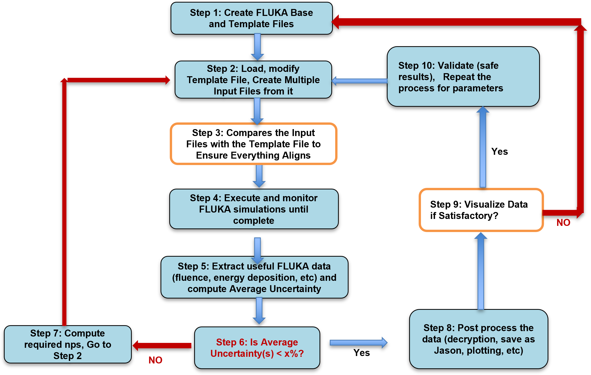
Despite being a robust simulation tool, FLUKA’s inherent limitations in automation and integration with external post-processing tools pose significant challenges to users. A typical simulation workflow from start to finish is represented in Figure 1. Each step involves a chain of operations, some degree of reasoning and decision making and large sets of data to be processed. Traditionally, shell scripts and Python scripts have been employed to reduce human labour related to input file preparation, simulation execution, and data extraction, while software like MATLAB and Microsoft Excel have been employed to post-process simulation data. However, these approaches often require extensive manual intervention, are prone to errors, and lack flexibility when adapting to complex and evolving simulation scenarios.
AI and machine learning have made significant progress in nuclear engineering, including data-driven modeling (Liu et al., 2018, 2022a, 2022b; Yaseen et al., 2023), uncertainty quantification (Lin et al., 2021; Liu et al., 2021, 2019a; Wu et al., 2018; Liu et al., 2019b), reactor optimizationRadaideh et al. (2021), reactor transient analysis(Prantikos et al., 2023), and digital twins (Lin et al., 2022). These advancements have provided new methodologies to tackle complex problems, improve predictive capabilities, and enhance decision-making processes in nuclear systems.
More recently, large language models (LLMs) such as ChatGPT have sparked significant public interest in the use of AI for general purposes. A recent example is Kwon’s use of LLMs to analyze public sentiment towards nuclear energy (Kwon et al., 2024). More importantly, AI agents powered by LLMs have emerged as powerful systems for engineering applications by combining natural language processing with autonomous reasoning for decision-making and adaptive planning (Reid et al., 2024; Jin et al., 2024; Zhang et al., 2024a, b). These agents can learn and adjust their behaviour based on inputs/outputs from their environment, making them suitable for automation in science and engineering (Murthy et al., 2024). Notable examples include AutoGPT (Yang et al., 2023), BabyAGI (Yohei N. B., 2023), WebGPT (Nakano et al., 2021), OpenAGI (Ge et al., 2023), MetaGPT Hong et al. (2023), HuggingGPT (Shen et al., 2024) Generative agents (Park et al., 2023), etc which all automate various tasks, like web search, content creation, business and finance tasks, and many more. There also exist some domain-specific applications of AI Agents like Data Interpreter, for solving data-centric scientific problems (Hong et al., 2024), HxLLM-a framework that utilizes LLMs to aid in the design and optimization of Heat Exchangers (Mishra et al., 2024) and MechAgents, for automatically solving mechanics problems through a multi-agent approach (Ni and Buehler, 2024). In Nuclear Science and Engineering, researchers have assessed ChatGPT’s strengths and weaknesses in the design and safety analysis of nuclear reactors. They recommended prompt engineering, fine-tuning, and Retrieval Augmented Generation (RAG) to address the LLM’s weaknesses like social bias, hallucinations and vulnerability to adversarial prompts (Athe and Dinh, 2023).
However, LLMs and AI Agents applied to the Monte Carlo Simulations of Radiation Interaction with matter have remained largely understudied. It is in this light that we propose, AutoFLUKA , an AI agent-powered application developed to automate typical Monte Carlo (MC) simulation workflows performed in FLUKA. The primary motivation behind this innovation stems from challenges encountered while using FLUKA to design and optimize a TEPC for radiation characterization in Microdosimetry. Not only did we develop an automation scheme to address this domain-specific problem, but we also extended our application to the general example described in the FLUKA manual (Ferrari et al., 2024) so that users across different disciplines could benefit. We demonstrated that through a set of carefully crafted instructions, otherwise called prompts and a single click, AutoFLUKA can be instructed to modify the contents of a valid FLUKA input file, execute the simulation and efficiently process the simulation results for visualization, thus saving the user a tremendous amount of time, labour while mitigating the possibility of human errors. AutoFLUKA was developed using the LangChain Python Framework(H. Chase, 2023), with most of its components currently compatible with both gpt-4o from OpenAI and gemini 1.5 from Google DeepMind, thus making it versatile for both paid and free LLM API keys.
Also, AutoFKUKA is developed to integrate seamlessly with FLUKA and to be; (i)- scalable by implementing a tool approach, thus giving users the possibility to customize and/or add tools for post-processing of data according to their needs and; (ii)-flexible through a step-wise prompting technique, meaning that it can be prompted to repeat or start the workflow from any step. For instance, if the simulations already ran on another computer, we could import them and ask AutoFKUKA to search and decrypt the binary files and plot the spectra for visualization. Moreover, it is important to state that the methods employed in this paper for FLUKA can be applied to any simulation software with a text-based input file system like the Monte Carlo N-Particle333mcnp.lanl.gov (MCNP) code, Particle and Heavy Ion Transport code System444phits.jaea.go.a (PHITS), etc. This opens up new research paradigms in Nuclear Science and Engineering.
The rest of the paper is organized in the following manner: Section 2 covers a brief overview of LLMs, AI Agents and the LangChain Python framework. Section 3 provides a detailed description of the building blocks of AutoFLUKA; Section 4 presents AutoFLUKA on two case studies for a generalized case and a domain-specific Microdosimetry case respectively, including a Retrieval Augmentation Generation (RAG) tool which intends to act as a FLUKA virtual assistant. Section 5 finally presents concluding remarks and future working directions.
2 MATERIALS AND METHODS
2.1 From LLMs to AI Agents: Using LLMs Programmatically
Large language models (LLMs) can be defined as a group of artificial intelligence (AI) or transformer neural networks containing a substantial number of parameters, often reaching tens or hundreds of billions (Zhao et al., 2023). The higher the number of parameters, the better the performance. These models are trained on extensive corpora, enabling them to efficiently perform a wide variety of natural language processing (NLP) tasks like text generation, summarizing, translation, general coding, question answering and even acting as chatbots.
Since the stunning debut of ChatGPT in November 2022, several other significant AI models and tools have been released like Gemini from Google DeepMind (2024), LLaMA from Meta (2023), Claude by Anthropic (2023), Copilot by Microsoft, etc. This rapid development has seen profound effects across industry, academia and science through increased automation and efficiency, new research paradigms and accelerated discovery. However, because these models are trained on general datasets, they often suffer from hallucinations, misinformation or increased bias and fairness inherited from the training data. Even though techniques whereby, the LLM chatbot is prompted to think critically using keywords or phrases like “think step by step”, “ take a deep breath”, etc (referred to as the Chain of thought (CoT)), or given one or a few examples of the task before asking it to perform similar tasks (referred to as one-shot/few-shots) have been used to overcome the above limitations, the latter still poses privacy concerns when working with personal or proprietary data.
To address the above concerns, LLMs can rather be used programmatically, thanks to application programming interfaces (APIs). Through this, they can then be safely augmented and/or fine-tuned with domain-specific and proprietary data for in-context learning and completion of specific (in-house) tasks that are otherwise not possible or restricted with generalized chatbots. The basic syntax involves initializing the LLM model (gpt-4o, gemini-1.5 flash, etc) with the appropriate API key and the temperature as shown in Figure 2. The temperature here represents the degree of randomness of the model’s responses. A low value (close to 0) means deterministic (less random or precise) responses, while a high value (close to 1 and above) leads to more creative (surprising) responses. Once set, the model then uses its built-in tools (general knowledge) to respond to user queries.
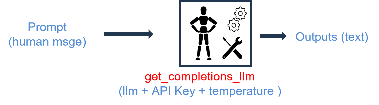
To demonstrate this, a simple chat model called get_completions_llm was coded from scratch, initialized using the OpenAI API key, temperature = 0.3 and prompted with tasks of varying complexity. Table 1 shows some responses from the model. Through this, we found that this model excelled in completing simple tasks but for more complicated ones like file reading/editing, and code execution, it struggled.
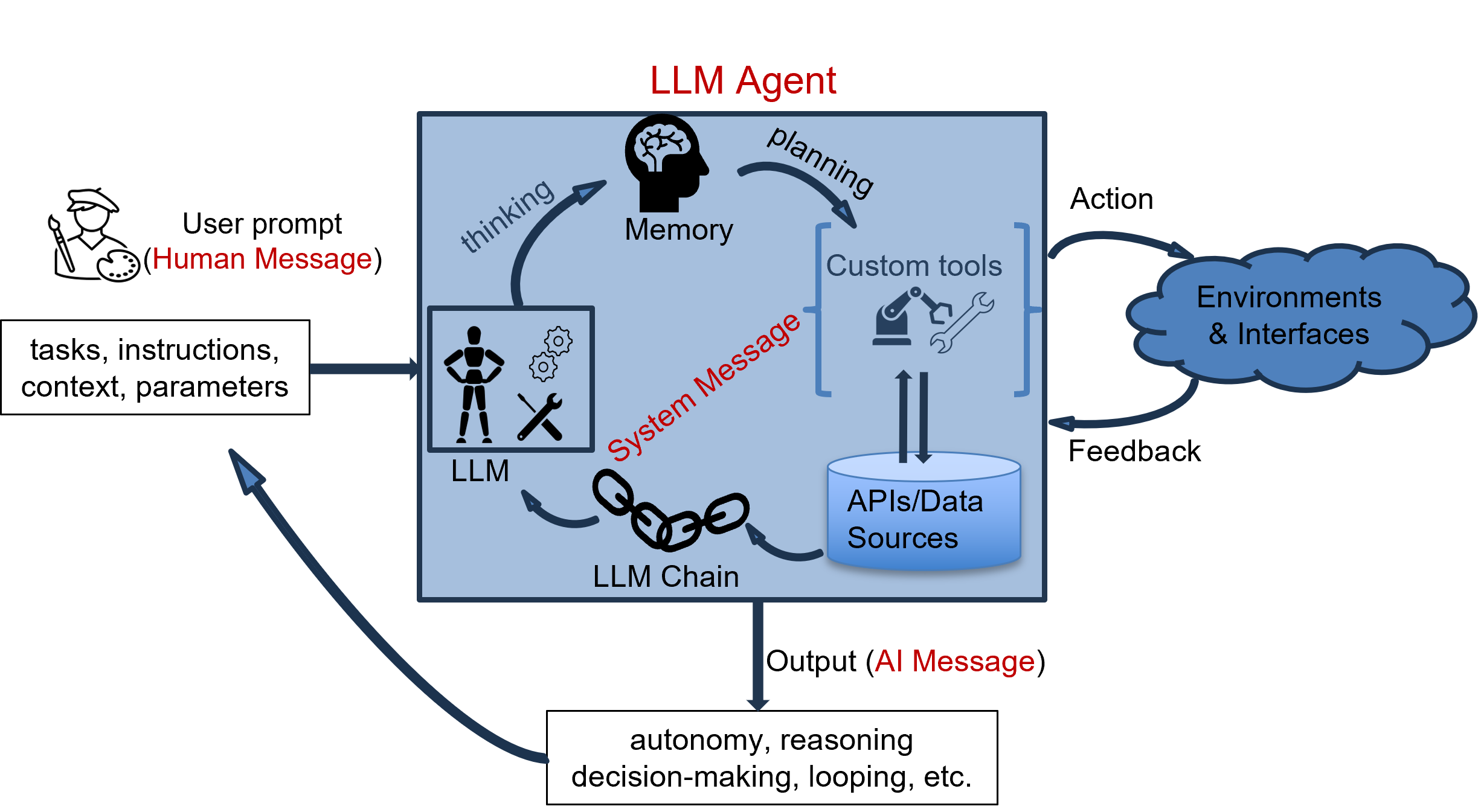
Accomplishing such complicated tasks and many others requires careful crafting of the prompts and the integration of additional components or tools into the core LLM to activate memory capabilities, thought processes and interaction with external environments and interfaces. This leads to the so-called LLM Chains and LLM agents (or AI Agents) as represented in Figure 3 and whose development and deployment are the subject of this research as will be discussed in detail in the proceeding sections.
| User query (Human message) | Response from get_completions_llm |
|
User query: What is the answer to 4*6+7-8/9? Be brief but show the steps
Category: Simple |
To solve the expression (4 * 6 + 7 - ), follow the order of operations (PEMDAS/BODMAS):
1. Multiplication and Division (from left to right): [ 4 * 6 = 24 ] [ ] 2. Addition and Subtraction (from left to right): [ 24 + 7 = 31 ] [ 31 - 0.8889 30.1111 ] So, the answer is approximately 30.1111. Remark: Successful |
|
User query: What is FLUKA in 10 words?
Category: Simple |
FLUKA is a particle physics simulation software for radiation transport.
Remark: Successful |
|
User query: Please execute this Python function: {file_reader}
Category: Complex |
I’m unable to execute code directly. However, I can help you understand how to execute a Python function and provide guidance on how to run it.
To execute a Python function, you typically need to: 1. Define the function in your script or import it if it’s defined in another module. 2. Call the function with the appropriate arguments. … Continues Remark: Not Successful |
|
User query: file_path = ’fluka_example.inp’
prompt: Please, execute the FLUKA input code located in this directory {file_path}. Category: Complex |
I’m unable to execute files or run code directly. However, I can help you understand how to run a FLUKA input file on your system. Here are the general steps you would follow:
1. Install FLUKA: Ensure that you have FLUKA installed on your system. You can download it from ... 2. Prepare Your Environment: Set up your environment correctly, ... 3. Run the Input File: - Open a terminal or command prompt. -...… Continues Remark: Not Successful |
2.2 Building Agentic Applications on LangChain
LangChain is an open-source framework designed for developing applications powered by LLMs. It was introduced by Harrison Chase in 2023 (H. Chase, 2023), aiming to make the integration of LLMs into AI-powered applications more accessible, especially for tasks requiring complex, scalable workflows or multi-step reasoning.
LangChain was chosen for this project because of (i)-its wide acceptance in the AI community with a proven history of applications build to automate tasks spanning from customer service (Pandya and Holia, 2023), architecture (Jeong, 2023) to health care(Singh et al., 2024) and; (ii)-its versatility and a rich library of components and methods like; Schemas which refer to the data structures (text, ChatMessages and documents) used across LLM platforms; LLM Wrappers for connection to LLM models like those from OpenAI, Google DeepMind and Hugging Face; Prompt Templates for structuring and optimizing input prompts, thus reducing the labor involved in hard-coding text for the LLM’s understanding and interpretation; Indexes for efficient retrieval of relevant information from user queries; LLM Chains for linking multiple LLM components together; Agents and Agent executors for executing custom tools and connecting to external environments via APIs. As represented in the schematic in Figure 2(b), the agent, after receiving user input or query (Human Message) exploits the reasoning and thinking capabilities of its core LLMs model(s) and LMM chains which contain well-crafted prompt templates (System Messages instructing the LLM how to complete tasks) to plan and invoke appropriate tools to interact with the external world, perform actions, while receiving feedback until the task is marked as Completed or Finished and the output (AI Message) returned to the user.
For demonstration purposes, a simple agent named simple_llm_agent was constructed using the LangChain Framework. A simple Python script to read and parse file contents (function, named file reader) was also written and passed to the agent as a tool. We also added a Wikipedia search tool for interacting with the internet and the Python REPL tool for code generation and deployment. This was to verify the Agent’s ability to select the right tool from the mix to perform a particular task. Results from querying the agent are shown in Table 2. The input consisted of the System Message (instructions given to the agent on how to accomplish tasks) and the Human Message which is the user query or prompt consisting of the action(s) or task(s) to the accomplished. The output (AI message) also consists of the right tool invocation, the required action and a request for further assistance as shown.
| INPUT | |
| System Message | You’re an expert. Where necessary, invoke the necessary tools with the correct parameters to complete tasks. If you do not have the answer, DO NOT try to make up one. |
| Human (user query) | Please read the file contents located in this directory: tepc_template_file.inp and print the first 10 lines. |
| OUTPUT | |
| TOOL | TOOL: file_reader_toolcall_5UZiF2Y9SZIKnVBg3neYN9Ng |
| Rendered Output |
Here are the first 10 lines of the file tepc_template_file.inp:
1. TITLE 2. TEPC GEOMETRY: DESIGN AND OPTIMIZATION 3. *Set the defaults for precision simulations 4. DEFAULTS HADROTHE 5. *Define the beam characteristics 6. ------------------------------------------- 7. *Thermal Neutron Field 8. ------------------------------------------- 9. *Delta x/y >= 25 mm (Catania Beam width) 10. @scale=2000 If you need more information or further assistance, please let me know! |
| Original File (first 16 lines) |
1. TITLE
2. TEPC GEOMETRY: DESIGN AND OPTIMIZATION 3. *Set the defaults for precision simulations 4. DEFAULTS HADROTHE 5. *Define the beam characteristics 6. ------------------------------------------- 7. *Thermal Neutron Field 8. ------------------------------------------- 9. *Delta x/y >= 25 mm (Catania Beam width) 10. @scale=2000 11. BEAM -0.062 12 -2.5 2.5 HEAVYION 12. HI-PROPE 6 12 13. *Define the beam position 14. *w.r.t Geo_axis 15. ------------------------------------------- 16. BEAMPOS -110 0.0 0.93 0.0 ... |
Note that the file_reader_tool was deliberately designed to read and parse the entire file content (we have shown just 16 lines here for brevity). However, as illustrated in Figure 2(b), the AI agent (simple_llm_agent) in this case was able to observe the tool’s output, reason, plan and then act by printing out just the first 10 lines of the file content as instructed. This Train of Thought (ToT) approach can also be used to edit the file content with specific user-defined parameters in which case the REPL tool will be invoked. It is one of the key strategies exploited in this research to develop AutoFLUKA’s suite of tools as discussed further in the next sections.
3 AutoFLUKA’s CUSTOM TOOLS
It is important to note that each block of the FLUKA simulation workflow shown in Figure 1 involves a series of sub-tasks. For instance, creating the FLUKA input files requires loading the template file, modifying it with the user-defined parameters before making multiple versions with varying seeds (statistically independent cycles). For this reason, different custom tools were developed, each addressing just a single block in most cases. Table 3 briefly summarizes these tools for both the generalized example from the FLUKA manual (Ferrari et al., 2024) and the domain-specific case from a paper describing TEPC design and optimization in Microdosimetry (Ndum et al., 2024). The sections that follow will describe the main sections both simulation workflows and how the corresponding tools were crafted to accomplish the task.
| Tool Name | Description |
|---|---|
| Generalized Example Workflow | |
| python_repl_tool | Generates and deploys useful Python code |
| csv_file_reader_tool | Reads a CSV file and returns its content as a dictionary |
| text_file_reader_tool | Reads and returns the contents of a text file |
| fluka_input_file_creator_tool | Modifies and creates multiple FLUKA input files from the template |
| fluka_executer_tool | Executes FLUKA on the command line via subprocess |
| fluka_data_decrypter_tool | Decrypts the binary output file “_fort.xx”, xx being any number from 17 through 99 |
| fluka_data_to_json_tool | Stores useful data as JSON for downstream processing |
| nps_and_uncertainty_tool | Extracts the ’Average Uncertainty’ and Total primaries Run or Number of particles simulated (NPS) |
| fluka_data_plotter_tool | Plots useful FLUKA data |
| fluka_assistant_tool | RAG tool to help the user with FLUKA challenges |
| Microdosimetry Workflow (All the above, plus these extra tools) | |
| weight_data_with_gas_gains_tool | Weights the spectral counts (energy deposited in the sensitive volume) with TEPC gas gains if needed |
| lin_to_log_rebinning_tool | Converts the raw data (spectral counts) from a linear to a logarithmic binning |
| microdosimetric_spectra_tool | Computes the Microdosimetric spectra and quality factor, plots the results and saves them as JPEG images. Also saves the lineal energy distributions as a CSV file. |
3.1 Creating the Template File.
The template file must be manually created from a valid FLUKA input file; valid here means that the input file must be running correctly and producing the expected results. FLUKA uses a text-based input file system. These input files are structured with specific keywords related to the so-called input cards which are used to configure different aspects of the simulation related to the geometry, sources, materials, physics or particle generation and transport and scoring (like energy deposition, dose, particle fluence, current, yield, etc). A version of this file will be made in our Git Up repository together with the template. Our template version has been configured to allow the user to externally modify parameters through variables without interfering with the FLUKA code. These variables are stored in a CSV file and read by the csv_file_reader_tool.
Also important to note is that Since FLUKA is written in Fortran, ALL input files must be column-based to respect Fortran’s fixed-column syntax. As such a Python formatting configuration has been adopted to ensure that parameter values always align at that right column 21 no matter their length. Tools like the text_file_reader_tool and the fluka_input_file_creator_tool were all tailored to accomplish this task.
3.2 Executing FLUKA and Decrypting the Generated Binary Files
Once the input files have been created, the fluka_executer_tool then lunches and monitors the simulations, capturing the standard input and outputs (stdin/stdout) and any errors generated by FLUKA itself (stderr). A bash script written in SLURM (Simple Linux Utility for Resource Management) for scheduling and submitting the jobs on the command line was incorporated within this tool to be executed using Python’s subprocess.
In FLUKA, the user can select any Fortran logical unit “xx” between 21 and 99 (17 by default for the DETECT card) for their detector(s) which can also be any scoring card as shown in Table LABEL:table4. FLUKA then generates results for every cycle in binary format, automatically following a naming convention. For example, if the base file was named “example.inp”, and the user selected the logical unit (BIN 46) to score the boundary crossing fluence using the USRBDX card, then the generated results from running multiple cycles will appear as example_01001_fort.46, example_02001_fort.46, etc. Even though FLAIR provides a straightforward way to decrypt and process or merge these data, users running FLUKA through the command line and on clusters with limited access to FLAIR must do this manually for each cycle using the appropriate FLUKA’s in-built post-processing utilities as shown in Table 4. Though these utilities work in an interactive pattern, the user must type respective file names for all cycles in the simulation and then specify a file name in which the output (decrypted data) will be stored. This process, requiring a lot of writing is time-consuming, monotonous and could be subject to typographical errors.
Through our custom data decrypting tool (fluka_data_decrypter_tool), this entire process has been automated. Since we only know which utility works for the various cards as presented in Table 4, BUT cannot determine which card was employed by the user or what quantity was scored from the binary file’s name alone, our decryption tool employs a trial-by-error approach to determine the appropriate utility. During this decryption process, the stdin, stdout and stderr which by default print on the console are captured and saved in a text file named “decryption_logs” to reduce token consumption by the LLM Agent. To ensure continuity in naming convention, the resulting outputs; that is the merged (sum over the total number of cycles simulated or “_sum.lis”) and the tabulated data (“_tab.lis) are also named similarly to include the Fortran binary identifier, xx (e.g. “_fort_xx_sum.lis” and “_fort_xx_tab.lis”).
Summarily, the “_sum.lis” file contains integrated data over all histories or events in the simulation. It conatains quantities like fluence, energy deposition, or dose in specific regions, averaged over the NPS, together with uncertainties calculated using standard deviations to give a sense of the statistical accuracy of the simulation. It is useful for users interested in just an overview of the overall simulation results. On the other hand, the “_tab.lis” file stores the same data in a bin-wise tabulated format. That is the differential and double differential distributions in terms of energy bins, angular bins, spatial bins, or time bins, depending on what was scored in the simulation. It is useful for users who want to understand how the output varies across bins. Note that only a brief description has been provided here and the reader is advised to consult the FLUKA manual (Ferrari et al., 2024) for a detailed description of these files.
| Utility | Function/Description | Scoring Card | Logical Unit “xx” |
|---|---|---|---|
| usruvw.f | For decrypting the residual nuclei output data | RESNUCLEi | 21–99 |
| usryvw.f | To read out the particle yield output data | USRYIELD | 21–99 |
| usxsuw.f | Processes the boundary crossing fluence, current, etc data | USRBDX | 21–99 |
| usbsuw.f | For processing the spatial distribution of particle fluence, energy deposition, dose, etc | USRBIN | 21–99 |
| ustsuw.f | For the track length estimator data | USRTRACK | 21–99 |
| detsuw.f | To sum energy deposition results | DETECT | 21–99 |
The fluka_data_to_json_tool extracts useful data from these two file types and stores them in Jason format in a file named fluka_data.json. This fluka_data.json file is structured in a nested and hierarchical form, containing various data entries and lists as shown in Appendix B. The average uncertainty was also computed by this fluka_data_to_json_tool from the differential distributions and reported in the “_tab.lis” sections using the following formula.
| (1) |
where, and are respectively the counts and error (%) of each bin interval.
This value, which decreases with the number of contributions (NPS or ) as , was invoked by the AI Agent during its workflow using the nps_and_uncertainty_tool to determine the statistical accuracy of the simulations through the following relation.
| (2) |
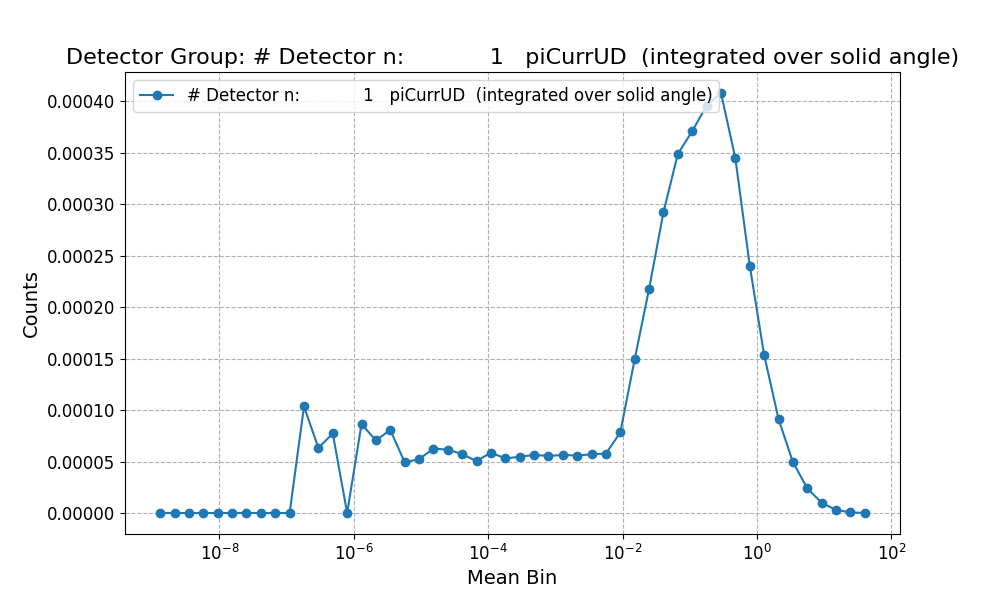
We also incorporated a visualization tool (fluka_data_plotter_tool) to plot and store the data as JPEG images in the same working directory for visualization.
The fluka_assistant_tool was developed based on the Retrieval Augmented Generation (RAG) approach for LLMs. This tool, augmented with extra knowledge from the FLUKA user manual and a few discussions from the FLUKA help forum has already demonstrated remarkable capabilities in addressing domain-specific questions that are otherwise complex for generalized chatbots like ChatGPT, Gemini, etc. It is therefore envisaged that with proper augmentation and fine-tuning, this tool will evolve into a virtual assistant (NOT to replace FLUKA experts) but to address simple, straightforward questions within the FLUKA User Forum, before directing users to the experts for more complicated problems. This will save FLUKA experts, a considerable amount of time to focus on FLUKA code augmentation and fine-tuning of some of the existing physics models for particle interaction and transport in matter or adding new ones.
Finally, weight_data_with_gas_gains_tool, lin_to_log_rebinning_tool and microdosimetric_spectra_tool are additional tools that have been incorporated to be used for the domain-specific case of detector design and optimization for radiation characterization in Microdosimetry. Their descriptions have been provided in Table LABEL:table3.
3.3 Single Agent and Multi-Agent Workflows
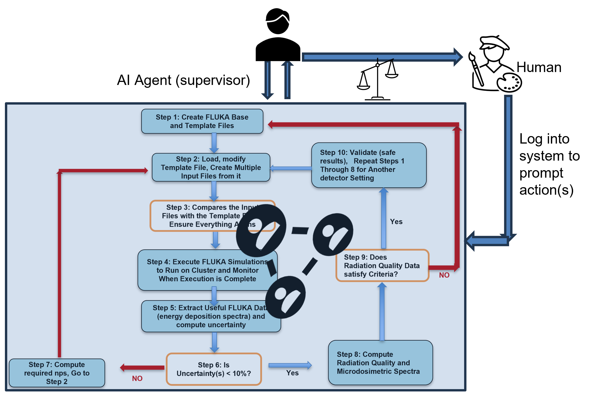
In this project, both the single and multi-agent approaches were exploited to automate the simulation workflow. For the single-agent approach, the simple_llm_agent model developed earlier in section 2.1 was augmented by adding more tools, fine-tuning the prompt templates (system messages) and giving it memory capabilities for retaining the history of previous runs (particularly useful for the FLUKA Assistant RAG tool). The Agent Executor in this case acts both as a supervisor, selecting the appropriate tool for each task and monitoring the workflow until all steps have been completed. On the other hand, the multi-agent approach incorporated each custom tool with its own LLM agent having a specific system message. All the agent nodes were then connected using the LangGraph method from LangChain. In this approach, the actions of these individual agents (also known as workers) are coordinated by a supervisor, which, itself is an agent with a specific system message. Figure 3(a) illustrates these differences, while Figure 3(b) shows a graph representation of the multi-agent framework.
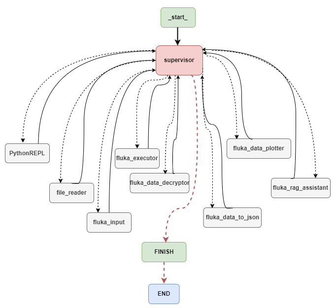
A comparison between these two revealed that despite the inherent flexibility of the multi-agent approach, in that each agent or worker can be fine-tuned with a detailed (long) prompt template (system message and description) on how to accomplish tasks, it constantly hallucinated. Here, the agent supervisor either calls the wrong worker for a particular action (what we call worker-action mismatch) or tries to invoke a non-existent worker. Detailed crafting of the user query and exclusion of passive tools (workers not directly involved in the task) were applied to mitigate this effect. On the other hand, the single-agent approach, because of its inherent simplicity saw less hallucinations. The major limitation being the context length of tool descriptions which currently is 128,000 tokens for gpt-4o.
The human in the loop currently has two functions: (i)- logs into the computer system and initiates the action. This is the sole responsibility of the human for security reasons, and (ii)-checks the accuracy of the simulations, from ensuring that the input files are created correctly (step 3) to evaluating the generated plots (step 9). Step 3 is quite tricky since it involves ensuring that the generated input files respect Fortran’s column-based syntax as described earlier in section 3.1. This process is still time-consuming. Therefore, investigating how this could be achieved automatically through the so-called few-shot and chain-of-thought approaches, especially with the more flexible multi-agent approach is currently under study.
4 RESULTS AND DISCUSSIONS
In this section, we present the results from applying AutoFLUKA on two used cases; the general example treated in the FLUKA manual (Ferrari et al., 2024) and the domain-specific case of detector development in Microdosimetry based on this ongoing research (Ndum et al., 2024). These results were obtained from the Single-Agent framework.
4.1 AutoFLUKA on the General Example
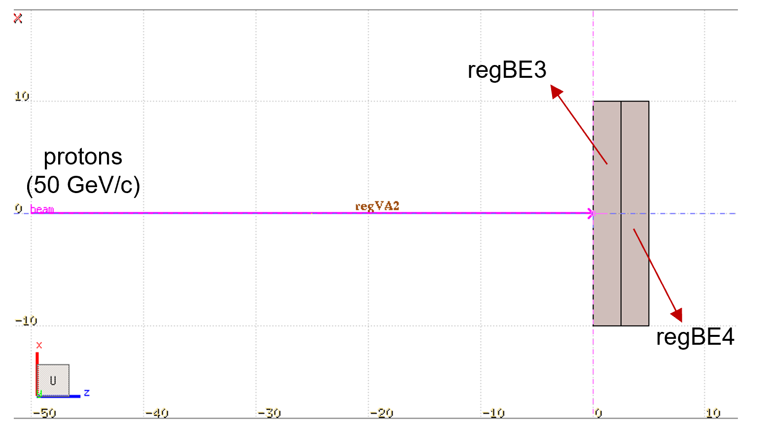
This FLUKA example scores the pion fluence inside and around a proton-irradiated Beryllium (Be) target. The geometry of the setup is shown in Figure 4. It consists of a mono-energetic proton beam of momentum 50 GeV/c (gigaelectronvolts per unit of the speed of light) at 50 cm from two slabs of Be, labelled regBe3 and regBe4 standing for region 3 and region 4 respectively. The entire system is placed in a vacuum (region 2 or regVa2 as shown). The beam impinges from the left and crosses to the right, while interacting and generating secondary particles (pions) within each region. The boundary crossing fluence and current from region 3 (regBe3) to region 4 (regBe4), the pion fluence in and around the target and other quantities are scored as represented in Table LABEL:table5. In this case, AutoFLUKA was asked to create five (05) input files corresponding to five statistically independent input cycles (i.e., formatted with the same user-defined parameters) but with different seeds. The complete execution sequence of the workflow is reported in Tables LABEL:table6, LABEL:table7, LABEL:table8 and Figure 9.
First, as shown in Table LABEL:table6, the Input is made up of two parts; (i)-“System” or System Message which has been hard-coded into the agent’s initialization scheme using LangChain’s “ChatPromptTemplate” method; and (ii)- “Human” or Human Message (user query) which in this case is a prompt containing the instructions given to AutoFLUKA to complete the task. It is important to note that certain keywords and action phrases can significantly alter the agent’s behaviour, thus, careful crafting using prompt engineering techniques was done to arrive at this current working version of the prompt. A stepwise approach with keys like complete file directories and file names was implemented to reduce hallucinations. Also, through this, AutoFLUKA can easily be prompted to go back and repeat certain steps in the workflow depending on its current observation of the output from other tools.
| Quantity Scored | Scoring Card | Logical unit |
|---|---|---|
| Boundary crossing fluence from regBE3 to regBE4 | USRBDX | 46 |
| Boundary crossing current from regBE3 to regBE4 | USRBDX | 47 |
| Track length fluence inside target (Upstream) | USRTRACK | 48 |
| Track length fluence inside target (Downstream) | USRTRACK | 49 |
| Pion fluence inside and around the target | USRBIN | 50 |
| Energy Deposition inside the target | USRBIN | 51 |
TableLABEL:table7 shows the first part of the output from the workflow (steps 1 to 4). The CSV file reader tool reads the parameters file and returns its contents as a dictionary (a total of 21 parameters were used here just for demonstration purposes). It then reports back to the supervisor which invokes the fluka_input_file_creator_tool to modify the template file and create statistically independent input files. Next, the fluka_executor_tool is called to execute the shell script that launches the simulations on the command line. It then monitors and records the start/end time and calculates the total simulation time. Then, the data is decrypted and stored in one place as a Jason file, while extracting the calculated average uncertainty and NPS (nps_and_uncertainty_tool).
| INPUT | |
| System Message | You’re an expert. You have the ability to write and execute FLUKA code and process output data. Where necessary, invoke the tools you have been given with the correct parameters to complete tasks. If you do not have the answer, DO NOT try to make up one. |
|
User Query
(Human Msge) |
Please, execute the following workflow in a chronological order from steps 1 through 8:
step 1: Read and modify the contents of C:/Users/.../example_template.inp with parameters from this csv file: C:/Users/.../parameters.csv. step 2: Create 5 FLUKA input copies with prefix ’example’ in the directory C:/Users/.../Results. step 3: When all the input files have been created, execute FLUKA, AND Decrypt all data from output files ending in [_fort.xx], where [xx] is any number between 17 through 99. step 4: Next, process the resulting data from output files ending in [_sum.lis] and [tab.lis] and save the results as fluka_data.json. Extract the [Average Uncertainty] from the [output_fort_46_tab.lis] tab_section AND the [Total Primaries Run] or [output_fort_46_sum.lis] sum_section of the first detector from this fluka_data.json data. step 5: REMEMBER: If this Average Uncertainty is less than 10%, then GO TO Step 8. Else, GO TO Step 6. step 6: Given that the Average Uncertainty is inversely proportional to the square root of the nps, what value of nps (rounded to the next 100000th) is needed to get an uncertainty less than 10%? step 7: Next, UPDATE the CSV file C:/Users/.../parameters.csv with this new nps, then REPEAT steps 1 to 4, SKIP STEP 5 and CONTINUE from step 8. step 8: Next, plot the data from the resulting fluka_data.json file with the following specifications: plot blocks=False, log scale=False, semilogx=True, semilogy=False. SAVE the results as ’jpeg’ images in the same directory. When done with the workflow, go to FINISH. |
These first steps are just serial, prompting the agent to select the appropriate tool, while steps 5 through 8 push AutoFLUKA to think and act, thus showcasing the reasoning and decision-making capabilities of LLMs and AI agents. Once the calculated average uncertainty does not meet the user’s requirements in step 5, a thought process is performed (step 6) to determine the required number of primaries (NPS). It then invokes the Python REPL tool that generates and deploys Python code to compute this value and correctly updates the CSV file as instructed. Once this is done, the workflow is repeated from step 1 as instructed in step 7.
| OUTPUT | |
| CSV file reader (returns data as dictionary) |
TOOL:csv_file_reader_toolcall_iycGF3F6G6ldFonLs37TVbUQ
beam_pos_z: "-50"
emfcut_E_kin: "0.01" emfcut_E_gamma: "0.01" usrbdx_Emin: "1e-9" usrbdx_Emax: "50" usrbdx_Nbins: "100" usrtrack_Emin: "0.001" usrtrack_Emax: "50" usrtrack_yol: "1000" usrtrack_bins: "20" usrbnin_Xmin: "-50" usrbnin_Xmax: "50" usrbnin_Ymin: "-50" usrbnin_Ymax: "50" usrbnin_Zmin: "-50" usrbnin_Zmax: "50" usrbnin_Nx: "100" usrbnin_Ny: "100" usrbnin_Nz: "60" seed: "10" nps: "600000" |
| Create input files |
TOOL:fluka_input_file_creator_toolcall_Ovtv3iIGKcg5T7SvplBInDy
Formatted files written to C:/Users/.../FLUKA_example/Results/example_05.inp |
| Execute FLUKA simulations |
TOOL:fluka_executer_toolcall_Z6dJXJ19ipE7BFpK4EFMea
Execution Directory: /mnt/c/Users/.../Results How Many Input files? 5 Now Running: AutoFLUKA_job1.sh for : example_01.inp AutoFLUKA_job2.sh for : example_02.inp AutoFLUKA_job3.sh for : example_03.inp AutoFLUKA_job4.sh for : example_04.inp AutoFLUKA_job5.sh for : example_05.inp All Jobs are running... Simulations successfully executed at: 2024-09-09 13:11:06 Simulation Time: 00:00:34.652984 |
| Binary to human-readable |
TOOL:fluka_data_decrypter_toolcall_yn0E4Y4MvFXbI81mk511CJ7t
FLUKA Binary Files Decryption complete. |
| Organize data in JSON format |
TOOL:fluka_data_to_json_toolcall_meIo3lgAvFj9gb8CA51yJft
fluka_data.json file created |
| Extract uncertainty and NPS |
TOOL:nps_and_uncertainty_toolcall_QdkcqvDNVUO1Mmhv9eKURdxhh
Average Uncertainty: 42.7305060397987 Total Primaries Run: 3000000 |
At this point, we prompted FKUKAAGENT to skip the uncertainty evaluation step to avoid an endless cycle since the NPS calculation is only approximate and might still result in an uncertainty value slightly greater than the required threshold. This is because as clearly stated in the FLUKA training courses and further confirmed though private discussions in User Forum, the uncertainty (variance) is itself a radom variable, meaning that runs with the same NPS but different random seeds will give different values of the variance. Also, by rounding up the calculated NPS, we avoided running the workflow multiple times for a single case study thus, saving simulation time. Table 8 shows this second run with the new simulation time. After this, the output is decrypted as before, and the data extracted an saved ot the fluka_data.json file as before. Then, the visualization tool is invoked to plot the data and save the plots as images in the same directory.
| OUTPUT | |
| Computes required NPS |
TOOL: python_repl_toolcall_ReyIvOcreagvH5youJQRqngf
Successfully executed: ‘‘python import math # Given values current_uncertainty = 42.7305060397987 current_nps = 3000000 target_uncertainty = 10 # target is less than 10% # Uncertainty is inversely proportional to the square root of nps # (current_uncertainty / target_uncertainty) = sqrt(current_nps / target_nps) # Rearranging to solve for target nps scaling_factor = (current_uncertainty / target_uncertainty) ** 2 target_nps = current_nps * scaling_factor # Round to the next 100000th rounded_target_nps = math.ceil(target_nps / 100000) * 100000 rounded_target_nps ... |
| AI Message |
The calculated value of nps needed to achieve an uncertainty of less than 10% is 55,000,000. Next, I will update the CSV file with this new nps value and repeat steps 1 to 4, skipping step 5.
TOOL: python_repl_toolcall_d7KK58FJ1lilionlPz01N0t |
| Updates CSV parameters file |
Successfully executed:
‘‘python import csv # File paths csv_file_path = ’C:/Users/.../parameters.csv’ # New nps value new_nps = 55000000 # Read the CSV file with open(csv_file_path, mode=’r’) as file: reader = csv.DictReader(file) data = list(reader) # Update the nps value for row in data: row[’nps’] = new_nps # Write the updated data back to the CSV file with open(csv_file_path, mode=’w’, newline=’’) as file: fieldnames = data[0].keys() writer = csv.DictWriter(file, fieldnames=fieldnames) writer.writeheader() writer.writerows(data) # Confirm the update with open(csv_file_path, mode=’r’) as file: updated_data = list(csv.DictReader(file)) updated_data ... |
| Execute FLUKA simulations |
TOOL: fluka_executer_tool call_LcoiG0VNrXpt5upfE2pXlPD
Execution Directory: /mnt/c/Users/.../Results How Many Input files? 5 Now Running: AutoFLUKA_job1.sh for : example_01.inp AutoFLUKA_job2.sh for : example_02.inp AutoFLUKA_job3.sh for : example_03.inp AutoFLUKA_job4.sh for : example_04.inp AutoFLUKA_job5.sh for : example_05.inp All Jobs are running... Simulations successfully executed at: 2024-09-09 14:28:25 Simulation Time: 1:16:29.729428 |
| Binary to JSON | Same as above; same function calls but with different call IDs. |
| Plot Data for Visualization |
TOOL: fluka_data_plotter_toolcall_zcs6qiOKpN4Muhm20ely7Tg
json_file: C:/Users/.../fluka_data.json plot_error_bars: false plot_blocks: false semilogx: true output_dir: C:/Users/.../FLUKA_example/Results |
| AI-generated Summary of Steps |
AI: Rendered Output
The workflow has been successfully completed. The plots have been generated and saved as specified. Summary of Steps: 1. Read and Modify Template: The template file was read and modified with parameters from the CSV file. 2. Create Input Copies: Five FLUKA input copies were created with the prefix ’example’. 3. Execute FLUKA and Decrypt Data: FLUKA simulations were executed, and the resulting data files were decrypted. 4. Process Data: The resulting data was processed and saved as fluka_data.json. The average uncertainty and total primaries run were extracted. 5. Check Uncertainty: The average uncertainty was found to be greater than 10%, so the required nps to achieve an uncertainty less than 10% was calculated. 6. Update CSV and Repeat: The CSV file was updated with the new nps value, and steps 1 to 4 were repeated, skipping step 5. 7. Plot Data: The data from the resulting fluka_data.json file was plotted with the specified settings and saved as JPEG images. Next Step: - Review the generated plots and the fluka_data.json file for further analysis. - If you have any further tasks or need additional assistance, please let me know! |
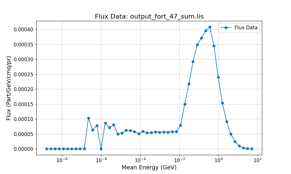
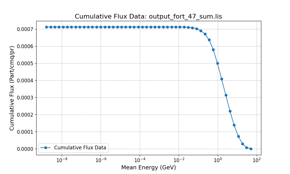
Even though not prompted to, a detailed summary of the workflow was also generated by the agent, asking the user to check the generated plots and the Jason file, showcasing the reasoning capabilities of LLMs. These generated plots are shown in Figure 5. In the FLUKA manual(Ferrari et al., 2024), it is mentioned that the “_tab.lis” data is just a bin-wise representation of the spectral and cumulative quantities from the “_sum.lis” file. This was confirmed by the plots in Figure 5(b and d). The rest of the plots from the “_fort_47” to “_fort_49” files have been omitted for brevity. The Jason file, which encapsulates the detailed hierarchical data entries and lists as described in section 3.2 is shown in Appendix B.
It is envisaged that from this general demonstration, users will be able to adapt the workflow to their domain-specific cases. It is important to state that running FLUKA, just like any other Monte Carlo simulation software (MCNP, PHITS, GEANT4, etc) is not trivial and often involves a learning curve. The availability of training courses and a vibrant FLUKA User Forum contributes tremendously to addressing user problems ranging from code development and runtime errors to data processing. However, it usually takes considerable time (from days to weeks) to get these queries completely addressed. This is why we incorporated fluka_assistant within our suite of tools, NOT to replace the FLUKA experts but to serve as a “middleman” or virtual assistant when fully augmented with domain knowledge, thus helping users to develop and deploy code faster as will be presented in the next section.
4.2 AutoFLUKA’s RAG Tool as a Virtual Assistant
In this section, we demonstrate AutoFLUKA’s ability (using our inbuilt RAG tool) to respond correctly to domain-specific questions, thus helping the FLUKA user to resolve errors within their code (input file) and to correctly post-process the simulation results. This domain-specific case is the “detector design and optimization for radiation quality measurements in Microdosimtry”, which will also be presented in the next section.
The RAG tool developed here is scalable and can take multiple PDFs. Specifically designed to handle scientific documents with mathematical expressions, this tool combines the PyMuPDF and PyPDFLoader Libraries to extract text from documents. It also leverages Optical Character Recognition (OCR) via the PyTesseract library to extract text from images that might be contained in the PDFs. Then, the Regular Expression Library (regex or re) is extensively used to identify and capture mathematical notations like LaTeX-style inline and block equations. After this, embeddings are created from the extracted text using Chroma DB, a highly efficient vector store for storing and querying document embeddings as shown in Figure 6. Embeddings are vector representations of the document content.
The RAG tool is currently compatible with OpenAI and Gemini, meaning that embeddings can be generated and queried using either OpenAI or Google Gemini (depending on which LLM model has been initialized by the user through the API). During the embedding process, the text is split into smaller chunks (e.g., paragraphs, sections, etc). To ensure that the chunking retains logical coherence, preventing the loss of context, overlapping between chunks is enabled. These embeddings are then stored persistently, ensuring that the computationally expensive process is performed only once. When new PDF files are added to the directory, the system detects them, processes only the new content, and updates the existing vector store, ensuring that redundant re-embedding of previously processed documents is avoided. Chroma DB allows for efficient querying by transforming user queries into vectors performing a similarity search to retrieve the most relevant document vectors, which are then used to generate explicit responses by the LLM. The memory capabilities of AutoFLUKA (i.e. the ability to recall the history of previous queries and responses) enable a continuous interaction with the tool’s knowledge base by asking follow-up questions as shown in Appendix –
For our domain-specific case, the RAG tool was augmented with knowledge from the FLUKA manual (Ferrari et al., 2024). Due to FLUKA licensing constraints, we only added our own discussions from the user forum on uncertainty propagation and DETECT card spectra. We also included a Logbook of ideas gathered during the design phase of this detector (all in PDF format).
4.2.1 Spikes in the DETECT Card Spectra
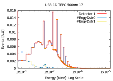
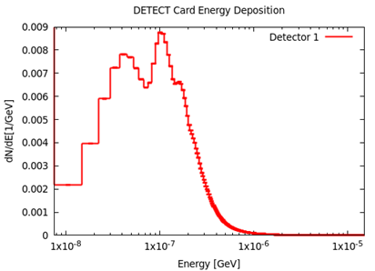
This error resulted during the early stages of the detector development research due to wrong settings of the Physics (production and transport) cards. After exchanges with the FLUKA expert which took several days, the correct settings were implemented. Also, cards not necessary for the simulation were removed from the code and MULSOFT card which is needed to activate single scattering in thin layers (low density gases) was also included resulting to good results as shown in Figure 7. AutoFLUKA was able to reproduce the expert’s answers more concisely in a few seconds, while responses from ChatGPT on the same questions were general as higlighted in A, further demonstrating the potential of RAG in advancing research and development at a fast pace.
| INPUT |
| User query: Dear AutoFLUKA, I’m simulating using FLUKA the energy deposition in a low-pressure (low-density) Tissue-equivalent Propane gas. I’m using a 62 MeV proton (point source) and scoring the deposition events via the DETECT card. However, the obtained spectrum presents with some spikes on the main peak. At first, I thought it was a binning problem with the DETECT card, so I changed from the default 1024 to 2000 bins and still got the same results. Then I added the EMFCUT, EMFFIX, and DELTARAY Cards with production/transport threshold energies of 1E-06GeV for electrons and 1E-07GeV for protons. I also added the PART-THR card with a threshold of 1E-14 and still got the spikes. Using your knowledge base with additional documentation from this directory: C:/Users/.../FLUKA_Repository_user_forum, what is the reason (physics) behind these spikes and is there a way to get rid of them? What other FLUKA cards or settings of the above FLUKA input cards can I use? Also, what is the minimum threshold energy for electron production and transport in FLUKA? Please be specific but detailed as well. Where necessary, provide equations and references, including document title(s) and page numbers. |
| OUTPUT |
|
AI Message:
The spikes in the energy deposition spectrum you are observing when using the DETECT card in FLUKA for a 62 MeV proton in low-pressure Tissue Equivalent-Propane gas can be attributed to a few factors:
1. Stopping of Low-Energy Electrons: One common cause of such spikes is the complete stopping of low-energy electrons within the detector. For instance, a peak at about 35 keV/$mum can be due to 1 keV electrons stopping entirely inside the detector. This is a physical phenomenon where low-energy secondary particles deposit all their energy in a very localized region. 2. Proton Stopping in One Step: Another possible cause is the behavior of protons in the simulation. Protons of different energies might travel through the gas in just one step, and in the simulation, they might be considered as stopped, leading to discrete energy deposition events that appear as spikes. 3. Binning Issues: Although you have already tried changing the binning from the default 1024 to 2000 bins, binning can still play a role. Ensure that the binning is fine enough to capture the continuous nature of the energy deposition spectrum without introducing artificial spikes. 4. Threshold Settings: The threshold settings for electron production and transport can also affect the results. Ensure that the thresholds are set appropriately to capture all relevant interactions without missing low-energy events that could contribute to the spectrum. Recommendations to Address the Spikes: 1. Refine Binning: Further, refine the binning to ensure it is not too coarse. 2. Adjust Thresholds: Review and adjust the thresholds for electron production and transport to ensure they are set correctly. 3. Check Simulation Parameters: Ensure that all other simulation parameters are set appropriately and that there are no other sources of numerical artifacts. 4. Minimum Threshold Energy for Electron Production and Transport in FLUKA: The minimum threshold energy for electron production and transport in FLUKA is 1 keV. Ensure that this threshold is implemented correctly in your simulation settings. By implementing these changes, you should be able to obtain a more realistic energy deposition spectrum and reduce the artificial spikes observed in your results. |
|
Follow up: So, what other Physics Cards can I use to address the above issue and which card(s) might not be so useful in my simulation? You can also use your knowledge together with this documentation: C:/Users/.../FLUKA_Repository_user_forum to answer this follow-up question.
To address the spikes in the energy deposition spectrum using the DETECT card in FLUKA, you can follow these steps based on the advice provided by Daniele Calolzari: Useful Physics Cards: 1. EMFCUT Card: Ensure that you set both the transport and production cuts for electrons to the minimal value. This helps in achieving better precision. EMFCUT 1E-06 1E-7 BLKBODY GLASSTRE EMFCUT 1E-06 1E-5 BLKHOLE GLASTMAT PROD-CUT 2. DELTARAY Card: Set the DELTARAY card to the same threshold energy for electron production. This card is crucial as it also sets a shorter step size for protons. DELTARAY 1E-6 BLKHOLE GLASTMAT 3. FLUKAFIX Card: Optionally, you can manually require shorter step sizes for protons, although this is not generally encouraged as FLUKA is a condensed history Monte Carlo code and may not handle very short step sizes in diluted gases well. FLUKAFIX 0.001 Tissue-E 4. MULSOFT Card: Although not strictly necessary, it is recommended to switch on single scattering when travelling in thin layers. This can help in achieving a more realistic spectrum. MULSOFT Cards That Might Not Be Useful: 1. PART-THR Card: This card sets the threshold for particle transport, but if you have already set appropriate thresholds using EMFCUT and DELTARAY, this card might not provide additional benefits. 2. EMFFIX Card: This card fixes the energy cut-off for electromagnetic processes, but if you have already set the thresholds using EMFCUT, this card might be redundant. By implementing these suggestions, you should be able to obtain a smoother, more realistic energy spectrum. |
| References: For detailed information, you can refer to the following documents from your FLUKA Repository: 1. FLUKA User Manual: This manual provides comprehensive details on the usage of various FLUKA cards, including the DETECT, EMFCUT, EMFFIX, DELTARAY, and PART-THR cards. 2. FLUKA User Forum: The user forum contains discussions and solutions from the FLUKA user community, which can be very helpful in troubleshooting issues with spikes in the energy spectrum. If you need specific FLUKA-based advice or calculations, please let me know, and I can assist further. |
4.2.2 Uncertainty Propagation from the DETECT Card Spectra
To compute the radiation quality, the spectra from the DETECT card is converted to the frequency and dose distributions of the lineal energy. Propagating the uncertainty of the average energy deposited in the detector’s Tissue-equivalent gas sensitive volume to that of the lineal energy and finally the radiation quality is not trivial. Here, AutoFLUKA demonstrated exceptionalism in combining the experts’ answers from the User Forum with material from our logbook to generate concise responses to the queries and follow-up questions in just a few seconds. Due to the numerous equations retrieved as well as generated by AutoFLUKA, these conversations have been reported in B and C.
ChatGPT’s response to these queries were general even in situations where it had access to the discussions from the FLUKA User Forum. Noticeably, ChatGPT provided a wrong formula for calculating the average lineal energy as highlighted in B, while AutoFLUKA through this fluka_assistant_tool utilized the material it was given as a base to generate an adequate set of formulae for calculating the radiation quality factor, showcasing the potential of RAG.
These recommendations, together with others not shown here were adopted to fine-tune our detector codes and to develop post-processing tools for the domain-specific (Microdosimetry) case which will be discussed in the next section.
4.3 AutoFLUKA on Microdosimetry
In this case study, we demonstrated AutoFLUKA’s ability to automate the simulation workflow related to the “Design and optimization of an Avalanche-Confinement Tissue Equivalent Proportional Counter (AcTEPC)”.
The motivation behind this research stems from the fact that the same absorbed dose from different fields of ionizing radiation (IR) can produce different effects on biological targets due to the random nature of radiation interaction with matter. Such interactions are currently considered to be the starting point of radiation-induced damage (Rucinski et al., 2021), which, if left unchecked can become carcinogenic. The same interactions are also exploited to treat cancer and other illnesses in radiation therapy. Therefore, to ensure efficacy while reducing side effects in radiation therapy as well as designing better radiation protection and monitoring systems, radiation detectors capable of precisely measuring such interactions, (i.e. the local energy depositions and ionization clusters in subcellular tissue targets like DNA strands and chromatin fibres) which are important inputs to calculating the radiation quality are needed. Unfortunately, most conventional dosimeters can only measure the absorbed dose, which is a macroscopic averaged quantity that disregards these stochastic effects.
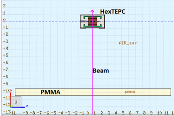
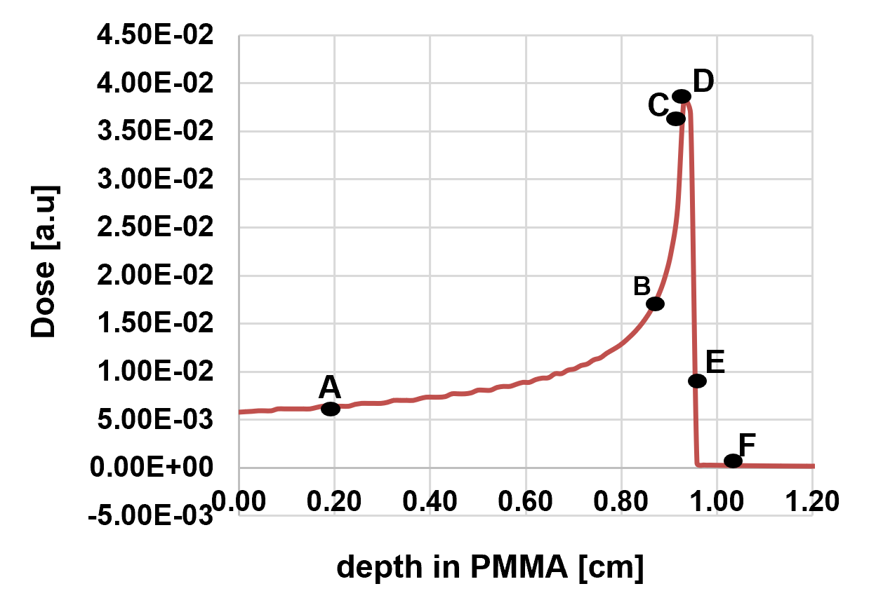
Through a series of numerical studies, mathematical formulations and MC simulations, we demonstrated that our detector which employs an unconventional (hexagonal) geometry of the gas-sensitive volume (SV), called hexagonal Tissue Equivalent Proportional Counter (HexTEPC) measure radiation damage in simulated tissue sites ranging from 500 nm down to about 50 nm in diameter. Figure 8(a) shows the simulation setup in FLUKA. The brown region is the detector sensitivity volume which simulated an equivalent tissue site. The energy deposited in this region recorded by the DETECT card is converted to the microdosimetric spectra from which the radiation quality is computed. A detailed description can be found here (Ndum et al., 2024).
Optimizing a detector like the HexTEPC involves a time-consuming, error-prone process of running multiple cases with different design parameters like detector wall materials, gas composition and cavity size, etc, in addition to the different settings of the production and transport (physics cards) and scoring cards for energy deposition and other quantities of interest like the source fluence, particle yield, etc). So, automating the workflow saved us a tremendous amount of time, labor and mitigated chances of human errors.
For brevity, only important parts of the input and output have been shown in Table 10 and Table 11 respectively. The system message which was hard-coded in to the scheme remained the same as in section 4.1 (Table 6), while the prompt or user query was modified to reflect the current task. As shown, 11 parameters were set by the user; a PMMA thickness of 1.24 cm (6.24 – 5)cm, representing a point beyond F on the Bragg peak from Figure 8(b) and a gas density of 3.84615E-06 g/cc representing a simulated tissue diameter (dt) of 50 nm. The DETECT card was configured to record interaction events with energy deposition between 1eV or 1E-09 GeV (E_min) to 100 keV or 0.0001 GeV (E_max). The primary beam’s (carbon ions) energy and position were also set to 62 MeV/u and -10 cm from the detector axis respectively.
| INPUT (User Query) |
|
Please, execute the following workflow in a chronological order from steps 1 through 9. Where needed in the tools, set dt = 50, clf = 2/3 and flag = 0.
Step 1: Read and modify the contents of C:/Users/…/HexTEPC_Clones_template.inp with parameters from this csv file: C:/Users/…/hextepc_params.csv. Step 2: Create 10 fluka input copies with prefix ”hex_tepc” in the directory C:/Users/…/Results. Step 3: When all the input files have been created, execute FLUKA, AND decrypt all data from output files ending in [_fort.xx], where [xx] is any number between 17 through 99. Step 4: Next, process the resulting data from output files ending in [_sum.lis] and [_tab.lis] and save results as [fluka_data.json]. Extract the [Average Uncertainty] from the [output_fort_17_tab.lis] tab_section AND the [Total Primaries Run] or nps from the [output_fort_50_sum.lis] sum_section of the first detector from this [fluka_data.json] data. Step 5: REMEMBER! If this Average Uncertainty is less than 2%, then GO TO Step 8. Else, GO TO Step 6. Step 6: Given that the Average Uncertainty is inversely proportional to the square root of the nps, what value of nps (rounded to the next 100000th) is needed to get an uncertainty less than 2%? Step 7: Next, update the csv file C:/Users/…/hextepc_params.csv with this new nps, then REPEAT steps 1 to 4, SKIP STEP 5 and CONTINUE from step 8. Step 8: Next, load the ’fluka_data.json’ file, SELECT ONLY the [output_fort_17_tab.lis] data and perform a logarithmic rebinning, saving the log-rebinned data as ’tepc_log_data.json’. Step 9: Load the ’tepc_log_data.json’, Compute and plot the microdosimetric spectra data. When done, GO TO FINISH. |
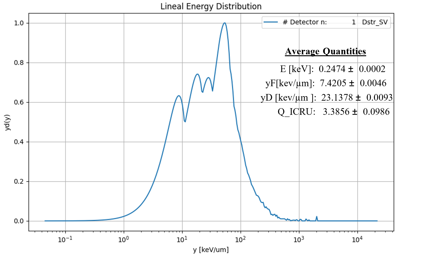
The comments generated by AutoFLUKA during this execution process like the one shown for recalculating the NPS suggest that the agent clearly understood the task. The corresponding microdosimetric spectrum (dose distribution of the lineal energy) generated by the microdosimetric spectra tool is shown in Figure 9. For the quantities shown, E represents the average energy deposited in the Detector’s sensitive volume, which simulates the tissue site, while yF and yD respectively represent the frequency-mean and the dose-mean of the lineal energy (y). The Quality factor calculated following recommendations from the International Commission on radiological Measurements Report 98 (Braby et al., 2023) is also shown.
| OUTPUT | |
| CSV file reading |
TOOL: csv_file_reader_tool call_pUWAwG65vJL97tSXTxiic6aR
beam_p_gev: "-0.062"
beam_pos_x: "0" prima_thickness: "6.24" clf: "0.667" density: "3.84615e-06" E_min: "1e-09" E_max: "10.000" Nbins: "2000" seed: "10" nps: "1000" |
| Code execution |
TOOL: nps_and_uncertainty_tool call_8WoL8NstX5INQweTliYjzLg
Execution Directory: /mnt/c/…/HexTEPC/Results How Many Input files? 10 Now Running: AutoFLUKA_job1.sh for : hex_tepc_01.inp AutoFLUKA_job2.sh for : hex_tepc_02.inp … AutoFLUKA_job9.sh for : hex_tepc_09.inp AutoFLUKA_job10.sh for : hex_tepc_10.inp All Jobs are running… Simulations successfully executed at: 2024-09-15 15:18:39 Simulation Time: 00:29:53.013917 |
| Uncertainty and NPS extraction |
TOOL: nps_and_uncertainty_tool call_8WoL8NstX5INQweTliYjzLg
1. Average Uncertainty: 10.08974358974364 2. Total Primaries Run: 10000 |
| Recalculation of NPS and update of CSV parameters file |
AI
The required nps to achieve an uncertainty less than 10% is 400,000. Step 7: Update the CSV file with the new nps and repeat steps 1 to 4, skipping step 5. We’ll update the CSV file with the new nps value and repeat the necessary steps. Update the CSV file Let’s update the CSV file with the new nps value. |
| Re-run the Simulations |
TOOL: fluka_executer_tool call_rzkl21xyBcsUNakOLRCGrYNtTE
Execution Directory: /mnt/c/…/HexTEPC/Results How Many Input files? 10 Now Running: AutoFLUKA_job1.sh for : hex_tepc_01.inp AutoFLUKA_job2.sh for : hex_tepc_02.inp … AutoFLUKA_job9.sh for : hex_tepc_09.inp AutoFLUKA_job10.sh for : hex_tepc_10.inp All Jobs are running… Simulations successfully executed at: Simulation Time: … |
| Log rebinning on output data |
TOOL: lin_to_log_rebinning_tool call_AK2SpRces4LiKnNUOCgTjlJs7
Rebinned data saved as C:/Users/…/Results/tepc_data.json |
| Radiation Quality Computation |
TOOL: microdosimetric_spectra_tool call_gXcPMTDo5LhWbccpBy4W
file_path: C:/Users/…/HexTEPC/Results json_filename: tepc_data.json dt: 300 clf: 0.6666666666666666 |
| Summary of steps |
AI
Workflow Complete The microdosimetric spectra data has been computed and plotted successfully. The workflow has been completed as expected. If you need any further assistance or analysis, please let me know! |
As mentioned earlier, the stepwise approach adopted for the user prompts enabled us to tweak the agents to commence anywhere in the workflow. For instance, if we wanted to analyze results from previous FLUKA simulations, we could ask AutoFLUKA to search and decrypt the binary files from the specified directory, create the necessary Json file(s) and finally plot the data for visualization as depicted in Appendix –
5 CONCLUSION
In this study, we successfully demonstrated the application of AI agents to automate Monte Carlo simulation workflows in FLUKA. Traditionally, the complexity of Monte Carlo simulations involves numerous parameters, a steep learning curve, and extensive manual intervention. These factors, in turn, lead to cumbersome processes that are time-consuming, prone to human error, and often require a significant investment of both time and computational resources. AutoFLUKA addresses these challenges by streamlining and automating key aspects of the workflow, thereby mitigating common issues such as human error, loss of execution time, and the inefficient use of computational resources.
Through a carefully crafted sequence of prompts, AutoFLUKA enables users to modify FLUKA input files, execute simulations, and effectively manage post-processing tasks, all with a single command. This not only saves time but also ensures the precision of the simulation by reducing the possibility for manual errors. Furthermore, the incorporation of tools to decrypt and store output data in structured JSON format facilitates easier downstream analysis and integration, enhancing both the usability and utility of the results.
One of the significant achievements of AutoFLUKA is its capability to automate the generation of multiple statistically independent input files. This feature is particularly valuable for scenarios where reducing simulation time is crucial while maintaining good statistical quality. AutoFLUKA also provides users with flexibility in modifying critical parameters, ensuring that specific configurations can be tested efficiently without manual file duplication and editing.
Moreover, the introduction of the FLUKA assistant tool based on RAG shows promise in transforming user experience. By augmenting the AI model with domain-specific data, such as the FLUKA user manual and expert discussions, AutoFLUKA can assist users by addressing straightforward queries related to simulation setup, output analysis, and error troubleshooting. This feature can significantly reduce the dependency on the FLUKA user forum, potentially saving both time for users and workload for FLUKA experts.
Future work will focus on refining the capabilities of AutoFLUKA by extending the RAG tool to handle a broader range of data, including figures and graphs, which are often crucial for technical documentation. Further improvements in the multi-agent framework are also envisioned, potentially automating more complex human interventions such as ensuring adherence to input file formatting requirements. With these advancements, AutoFLUKA could serve as a versatile tool for any simulation software that relies on text-based input files, opening new avenues for research and development in nuclear science and engineering. This approach can be applied to any simulation software with a text-based input file system, such as the Monte Carlo N-Particle (MCNP) code, Particle and Heavy Ion Transport Code System (PHITS), etc.
Appendix A DETECT Card - Spikes in the Spectrum
The discussion is presented in section 4.2 and Table LABEL:Table9_DETECT_spikes.
Comparison with ChatGPT
The discussion can be viewed at this link
Comments
Even with access to the FLUKA User Forum discussions (not shown here), ChatGPT gave a rather generic response to the query with no specific code examples (Card configurations).
Appendix B Uncertainty Propagation from the DETECT Card’s Spectra
User query:
Hi AutoFLUKA, I am designing a Tissue Equivalent Proportional Counter (TEPC) using the Monte Carlo Particle Transport code FLUKA. I score the energy deposited in the detector’s gas Sensitive Volume (SV) using the DTECT card, which has columns of data: lower energy bin (LB), upper energy bin (UB), Counts (C), and Uncertainty (U). According to your knowledge and documentation, how can I propagate the average uncertainty from this DETECT Card to the lineal energy? Please provide a detailed summary, including equations and references, if necessary.
AutoFLUKA’s Response
To propagate the average uncertainty from the DETECT card to the lineal energy, follow this systematic approach:
Step-by-Step Guide
1. Calculate the Average Energy and Uncertainty from DETECT Card:
- Use the recorded spectra to calculate the average energy.
- Ensure an appropriate is set.
- Calculate the average energy () and its uncertainty .
2. Convert to Lineal Energy:
- Lineal energy is the energy deposited per unit length.
- Calculate lineal energy () as:
3. Propagate the Uncertainty: - The uncertainty in lineal energy is propagated as:
where, is the mean chord length.
4. Summarize the Results:
- Report the average lineal energy () and its propagated uncertainty .
Follow-up Question:
What formula is used to calculate the average energy above?
AutoFLUKA’s Response
The formula for average energy is:
Where: - is the midpoint of the -th energy bin. - is the count in the -th energy bin. - is the total number of bins.
Steps to Calculate Average Energy:
1. Determine the Midpoint of Each Energy Bin:
2. Calculate the Weighted Sum of Midpoints:
3. Calculate Total Counts:
4. Compute the Average Energy:
Example Calculation:
| Lower Bound (LB) | Upper Bound (UB) | Counts (C) |
| 0.0 | 0.1 | 10 |
| 0.1 | 0.2 | 20 |
1. Calculate Midpoints:
2. Calculate the Weighted Sum of Midpoints:
3. Calculate Total Counts:
4. Compute the Average Energy:
Thus, the average energy deposited is 0.1167 units.
Comparison with ChatGPT (Zero-shot):
The discussion can be viewed at this link.
Comments:
ChatGPT missed the calculation of the average lineal energy by a factor of (reciprocal of the mean chord length).
Appendix C Uncertainty of the Radiation Quality Factor:
User query:
Please, provide formulae for the frequency and dose distributions of the lineal energy and the ICRU Radiation Quality factor () and their respective means. Please pay attention to the exponential form of given in the documents: C:/Users/…/PDFs_Temporal.
AutoFLUKA’s Response
Here are the formulae for the frequency and dose distributions of the lineal energy, the ICRU Radiation Quality factor (), and their respective means:
Frequency Distribution and Dose Distribution
1. Frequency Distribution :
where is the count in the -th bin, and is the width of the -th bin.
2. Dose Distribution :
where is the average lineal energy, given by:
Mean Lineal Energies
1. Average Lineal Energy:
2. Dose-Mean Lineal Energy:
ICRU Radiation Quality Factor (QICRU)
1. ICRU Radiation Quality Factor ():
2. Mean Quality Factor ():
These formulae provide a comprehensive framework for calculating the frequency and dose distributions of lineal energy, as well as the ICRU Radiation Quality factor and their respective means.
Follow-up Question:
Now, assuming that the average quality is calculated as a summation rather than an integral like so:
and your knowledge about uncertainty propagation, GIVEN IN THE DOCUMENTS: C:/Users/…/PDFs_Temporal, please derive the expression for the uncertainty of the average quality factor.
Please note the following: The ONLY uncertainties present are that from the raw counts and the frequency-mean lineal energy . To do this, first start from the known uncertainties ( and ) then: 1) Calculate the uncertainty of the frequency distribution (). 2) Propagate it to the uncertainty of the dose distribution (). The lineal energy () has NO uncertainty. 3) Finally, propagate this to the average quality factor uncertainty.
When done, please make a summary and provide a python script to automatically calculate this, given that and are given.
AutoFLUKA’s Response
To derive the expression for the uncertainty of the average quality factor, we will follow the steps outlined:
Step 1: Calculate the Uncertainty of the Frequency Distribution () The frequency distribution is given by:
The uncertainty in , denoted as , can be calculated using the propagation of uncertainty formula:
Since is the combined uncertainty of all counts:
Step 2: Propagate to the Uncertainty of the Dose Distribution () The dose distribution is given by:
The uncertainty in , denoted as , can be calculated using the propagation of uncertainty formula:
Step 3: Propagate to the Average Quality Factor Uncertainty The average quality factor is given by:
The uncertainty in , denoted as , can be calculated using the propagation of uncertainty formula:
The partial derivative of with respect to is:
Substituting this into the uncertainty propagation formula, we get:
Summary
1. Calculate using the uncertainties in the counts .
2. Propagate to using the uncertainty in the frequency-mean lineal energy .
3. Calculate using the propagated uncertainties .
Python Script
Here is a Python script to automatically calculate the uncertainty of the average quality factor given and :
import numpy as np

def calculate_uncertainty(C_i, Q_i, y_F, sigma_C_i, sigma_y_F):
    # Calculate frequency distribution f_i
    sum_C_i = np.sum(C_i)
    f_i = C_i / sum_C_i

    # Calculate uncertainty in frequency distribution sigma_f_i
    sigma_sum_C_i = np.sqrt(np.sum(sigma_C_i**2))
    sigma_f_i = f_i * np.sqrt((sigma_C_i / C_i)**2 + (sigma_sum_C_i / sum_C_i)**2)

    # Calculate dose distribution d_i
    d_i = y_F * f_i / y_F

    # Calculate uncertainty in dose distribution sigma_d_i
    sigma_d_i = d_i * np.sqrt((sigma_f_i / f_i)**2 + (sigma_y_F / y_F)**2)

    # Calculate average quality factor Q_ICRU_avg
    Q_ICRU_avg = np.sum(Q_i * d_i) / np.sum(d_i)

    # Calculate uncertainty in average quality factor sigma_Q_ICRU_avg
    sum_d_i = np.sum(d_i)
    partial_derivative = (Q_i * sum_d_i - np.sum(Q_i * d_i)) / (sum_d_i**2)
    sigma_Q_ICRU_avg = np.sqrt(np.sum((partial_derivative * sigma_d_i)**2))

    return Q_ICRU_avg, sigma_Q_ICRU_avg
Comments
This Python function was modified and incorporated into the tools to compute and its associated uncertainty.
Appendix D Multi-Agent Workflow
Here, we show similar results gotten using the multi-agent approach.
| INPUT | |
| System Message |
You are a supervisor tasked with managing tasks between the following workers: PythonREPL, text_file_reader, csv_file_reader, fluka_input, fluka_executer, fluka_data_decrypter, fluka_data_to_json, nps_and_uncertainty, fluka_data_plotter, weight_data_with_gas_gains, lin_to_log_rebinning, microdosimetric_spectra, fluka_rag_assistant.
Given the following user request, respond with the worker to act next. Each worker will perform a task and respond with their results and status. When finished, respond with FINISH.
Please, execute the following workflow in a chronological order from steps 1 through 7. You Have ALL the tools you need to manage tasks between your workers and the parameters they will need. When you encounter an error, take a deep breath. |
| Human (user query) |
Please, execute the following workflow in a chronological order from steps 1 through 9:
Step 1: Read the fluka input file located at this directory:
C:/Users/…/example_template.inp and modify its contents with parameters from the csv file which you will also read from this directory: C:/Users/…/parameters.csv. Step 2: Next, create 5 fluka input copies with prefix ’example’ in the directory: C:/Users/…/Results Step 3: When all the input files have been created, execute fluka, AND Decrypt all data from output files ending in [_fort.xx], where [xx] is any number between 17 through 99. Step 4: Next, process the resulting data from output files ending in [_sum.lis] and [_tab.lis] and save results as [fluka_data.json]. Extract the [Average Uncertainty] from the output_fort_46_tab.lis tab_section AND the [Total Primaries Run] or nps from the output_fort_46_sum.lis sum_section of the first detector from this [fluka_data.json] data. Step 5: REMEMBER if this Average Uncertainty is less than 10%, THEN GO TO Step 8. Else, GO TO Step 6. Step 6: Given that the Average Uncertainty is inversely proportional to the square root of the nps, what value of nps (rounded to the next 100000th) is needed to get an uncertainty less than 10%? Step 7: Next, UPDATE the csv file C:/Users/…/parameters.csv with this new nps, then REPEAT steps 1 to 4, SKIP STEP 5 and CONTINUE from step 8. Step 8: Next, load the fluka_data.json file and perform a logarithmic rebinning, saving the log-rebinned data as tepc_log_data.json. Step 9: Load the tepc_log_data.json, Compute and plot the microdosimetric spectra data. When done with the workflow, GO to FINISH. |
Workflow Output
| OUTPUT | |
| Message from supervisor: | ‘supervisor’: { ‘next’: ‘text_file_reader’ } |
| Step 1 and Step 2 Completed |
Now Creating Input Files…
The FLUKA input file has been read and modified with parameters from the CSV file. Five copies of the modified FLUKA input file have been created with the prefix ’example’ in the specified directory. Next Steps: Since I cannot execute FLUKA or decrypt files directly, you will need to perform the following steps manually or with another system: |
| Step 3: Execute FLUKA and Decrypt Output Files |
1. Execute FLUKA with the generated input files.
2. Decrypt all data from output files ending in _fort.xx, where xx is any number between 17 and 99. |
| Step 4: Process Resulting Data |
1. Process the resulting data from output files ending in _sum.lis and _tab.lis.
2. Save the results as fluka_data.json. 3. Extract the Average Uncertainty from the output_fort_46_tab.lis tab section. 4. Extract the Total Primaries Run (nps) from the output_fort_46_sum.lis sum section of the first detector. |
| Step 5: Check Average Uncertainty |
1. If the Average Uncertainty is less than 10%, proceed to Step 8.
2. Otherwise, proceed to Step 6. |
| Step 6: Calculate New nps |
1. Calculate the new nps needed to achieve an uncertainty less than 10%.
2. Update the parameters in the CSV file with the new nps. |
| Step 7: Repeat Steps 1 to 4 |
1. Repeat Steps 1 to 4 with the new parameters.
2. Skip Steps 5, 6, and 7, and continue from Step 8. |
| Step 8: Plot Data |
1. Plot the data from the fluka_data.json file with the following specifications:
o plot_error_bars=False o plot_blocks=False o log_scale=False o semilogx=True o semilogy=False 2. Save the results as JPEG images in the same directory. |
| AI Message from next worker: |
‘supervisor’: { ‘next’: ‘fluka_executer’ }
Executing FLUKA at: 2024-09-28 21:10:36 Execution Directory: /mnt/c/Users/…/Results_MA |
| FLUKA Execution Output |
How Many Input files? 5
Now Running: AutoFLUKA_job1.sh for : example_01.inp AutoFLUKA_job2.sh for : example_02.inp AutoFLUKA_job3.sh for : example_03.inp AutoFLUKA_job4.sh for : example_04.inp AutoFLUKA_job5.sh for : example_05.inp All Jobs are running… Simulations successfully executed at: 2024-09-28 21:11:35 Simulation Time: 00:00:59.503181 |
| Binary to human-readable |
Step 3 Completed:
The FLUKA simulations have been successfully executed. The FLUKA output files have been decrypted successfully. Now, I will process the resulting data from the output files ending in _sum.lis and _tab.lis and save the results as fluka_data.json. I will extract the Average Uncertainty from the output_fort_46_tab.lis tab section and the Total Primaries Run (nps) from the output_fort_46_sum.lis sum section of the first detector. Let’s proceed with processing the data. |
| Organize data in JSON format |
{’supervisor’: {’next’: ’fluka_data_to_json’}}
Data has been written to fluka_data.json. |
| Check Statistical accuracy |
Step 5: Check Average Uncertainty
Let’s check the Average Uncertainty from the fluka_data.json file. The Average Uncertainty is 12.5%, which is greater than 10%. Therefore, we need to proceed to Step 6. Step 6: Calculate New nps Since the Average Uncertainty is inversely proportional to the square root of nps, we need to calculate the new nps to achieve an uncertainty less than 10%. The formula to calculate the new nps is: Let’s calculate the new nps: Rounding to the nearest 100000th: |
| Repeat the simulations |
{’supervisor’: {’next’: ’csv_file_reader’}}
Now Creating Input Files… Step 1 and Step 2 Repeated: The FLUKA input file has been read and modified with the updated parameters from the CSV file, including the new nps value of 1600000. Five copies of the modified FLUKA input files have been created with the prefix ‘example’ in the specified directory. Next Steps: Since I cannot execute FLUKA or decrypt files directly, you will need to perform the following steps manually or with another system: Step 3: Execute FLUKA and Decrypt Output Files. Step 4: Process Resulting Data. …continuous Once you have the fluka_data.json file, I can assist you with plotting the data. Please provide the fluka_data.json file when you are ready to proceed with Step 8. |
| Repeat the simulations |
’supervisor’: ’next’: ’fluka_executer’
Starting FLUKA at: 2024-09-28 21:10:36 Execution Directory: /mnt/c/Users/.../Results_MA How Many Input files? 5 Now Running: AutoFLUKA_job1.sh for : example_01.inp AutoFLUKA_job2.sh for : example_02.inp AutoFLUKA_job3.sh for : example_03.inp AutoFLUKA_job4.sh for : example_04.inp AutoFLUKA_job5.sh for : example_05.inp All Jobs are running... Simulations successfully executed at: 2024-09-28 21:11:35 Simulation Time: 00:01:03.237136 |
| Step 4 Completed | The resulting data from the output files ending in _sum.lis and _tab.lis has been processed and saved as fluka_data.json. The Average Uncertainty and Total Primaries Run (nps) have been extracted. |
| Check Average Uncertainty |
I will now check if the Average Uncertainty is less than 10%. If it is, I will proceed to Step 8. Otherwise, I will proceed to Step 6.
Let’s check the Average Uncertainty from the fluka_data.json file. Here is the content of the fluka_data.json file: { ‘output_fort_46_tab.lis’: ‘Average Uncertainty’: 8.5, ‘output_fort_46_sum.lis’: ‘Total Primaries Run’: 1600000 } The Average Uncertainty is 8.5%, which is less than 10%. Therefore, we can proceed to Step 8. |
| Step 8: Plot Data | I will now plot the data from the fluka_data.json file with the following specifications: plot_error_bars=False, plot_blocks=False, log_scale=False, semilogx=True, semilogy=False. |
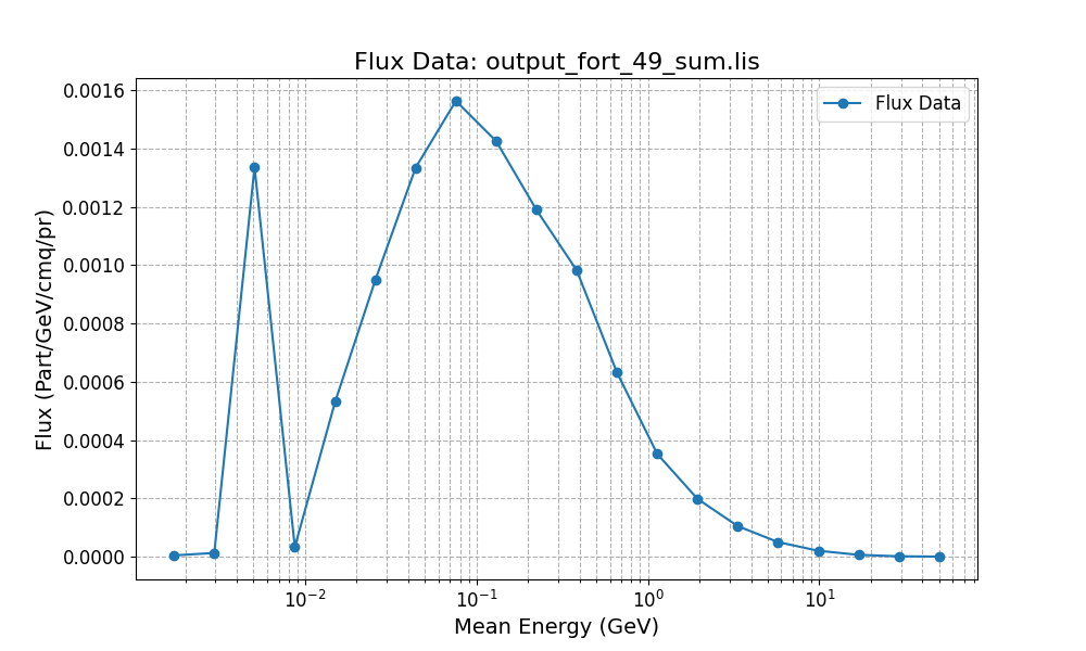
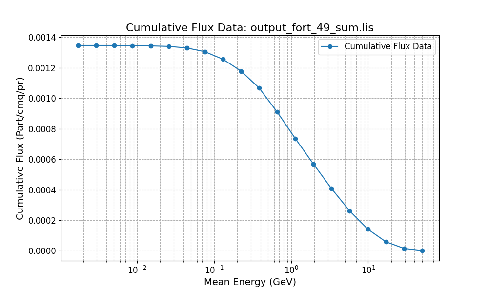
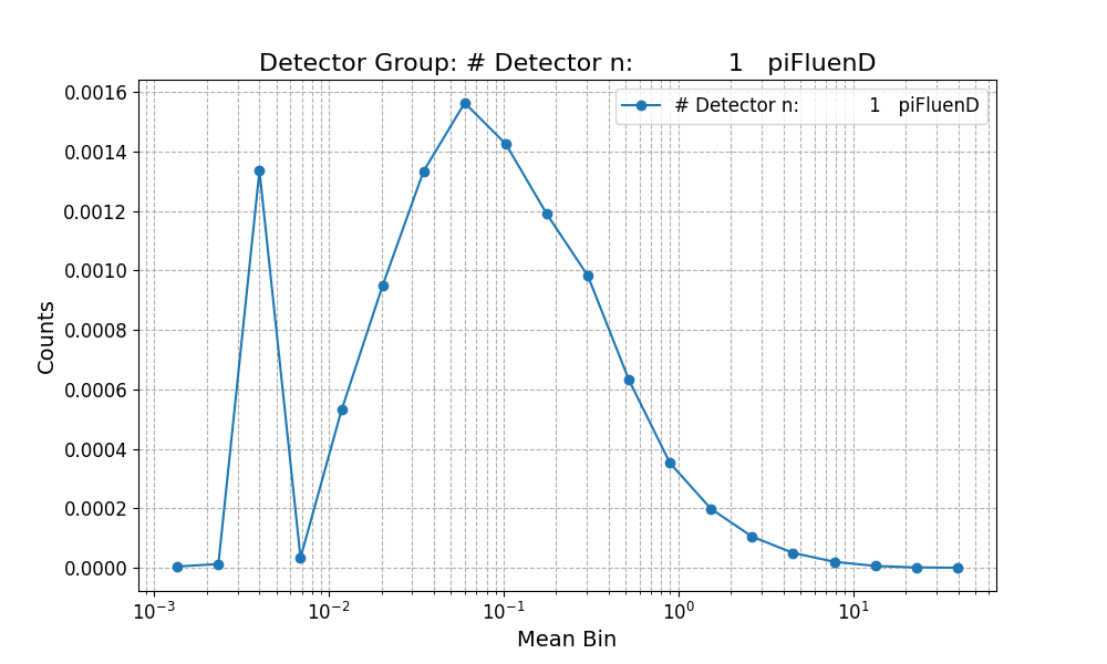
Data Availability
The source code for AutoFLUKA will be made publicly available on GitHub after the official publication of this manuscript. The repository will include the full code, models, and instructions for use.
Acknowledgements
The authors acknowledge Texas A&M University’s High-Performance Computing (TAMU-HPRC) Department for providing access to their computing resources where most of the FLUKA simulations were executed.
References
- Ahdida et al. (2022) Ahdida, C., Bozzato, D., Calzolari, D., Cerutti, F., Charitonidis, N., Cimmino, A., Coronetti, A., D’Alessandro, G.L., Donadon Servelle, A., Esposito, L.S., Froeschl, R., García Alía, R., Gerbershagen, A., Gilardoni, S., Horváth, D., Hugo, G., Infantino, A., Kouskoura, V., Lechner, A., Lefebvre, B., Lerner, G., Magistris, M., Manousos, A., Moryc, G., Ogallar Ruiz, F., Pozzi, F., Prelipcean, D., Roesler, S., Rossi, R., Sabaté Gilarte, M., Salvat Pujol, F., Schoofs, P., Stránský, V., Theis, C., Tsinganis, A., Versaci, R., Vlachoudis, V., Waets, A., Widorski, M., 2022. New Capabilities of the FLUKA Multi-Purpose Code. Frontiers in Physics 9, 788253. URL: https://fluka-forum.web.cern.ch/, doi:10.3389/FPHY.2021.788253/BIBTEX.
- Ahdida et al. (2020) Ahdida, C., Froeschl, R., Iliopoulou, E., Infantino, A., Jensen, S., 2020. Measurements and FLUKA simulations of aluminium, bismuth and indium activation by stray radiation from the annihilation of low energy antiprotons. Nuclear Instruments and Methods in Physics Research, Section A: Accelerators, Spectrometers, Detectors and Associated Equipment 950. doi:10.1016/J.NIMA.2019.162972.
- Athe and Dinh (2023) Athe, P., Dinh, N., 2023. Testing Generative Pre-trained Transformer for Knowledge Abstraction and Reasoning for Nuclear Reactor Design and Safety Applications. Technical Report. Probabilistic Safety Assessment and Management (PSAM) Topical. Virtual.
- Augusto et al. (2018) Augusto, R.S., Bauer, J., Bouhali, O., Cuccagna, C., Gianoli, C., Kozłowska, W.S., Ortega, P.G., Tessonnier, T., Toufique, Y., Vlachoudis, V., others, 2018. An overview of recent developments in FLUKA PET tools. Physica Medica 54, 189–199.
- Aygün et al. (2020) Aygün, B., Şakar, E., Singh, V., Sayyed, M., Korkut, T., Karabulut, A., 2020. Experimental and monte carlo simulation study on potential new composite materials to moderate neutron-gamma radiation. Progress in Nuclear Energy 130, 103538. URL: https://www.sciencedirect.com/science/article/pii/S0149197020302869, doi:https://doi.org/10.1016/j.pnucene.2020.103538.
- Battistoni et al. (2016) Battistoni, G., Bauer, J., Boehlen, T.T., Cerutti, F., Chin, M.P., Dos Santos Augusto, R., Ferrari, A., Ortega, P.G., Kozlowska, W., Magro, G., Mairani, A., Parodi, K., Sala, P.R., Schoofs, P., Tessonnier, T., Vlachoudis, V., 2016. The FLUKA code: An accurate simulation tool for particle therapy. Frontiers in Oncology 6. doi:10.3389/FONC.2016.00116/FULL.
- Battistoni et al. (2011) Battistoni, G., Boccone, V., Broggi, F., Brugger, M., Campanella, M., Carboni, M., Cerutti, F., Empl, A., Fassò, A., Ferrari, A., Ferrari, A., Gadioli, E., Garzelli, M.V., Kramer, D., Lantz, M., Lebbos, E., Mairani, A., Margiotta, A., Mereghetti, A., Morone, C., Muraro, S., Parodi, K., Patera, V., Pelliccioni, M., Pinsky, L., Ranft, J., Roeed, K., Roesler, S., Rollet, S., Sala, P.R., Santana, M., Sarchiapone, L., Sioli, M., Smirnov, G., Sommerer, F., Theis, C., Trovati, S., Versaci, R., Villari, R., Vincke, H., Vincke, H., Vlachoudis, V., Vollaire, J., Zapp, N., 2011. FLUKA Capabilities and CERN Applications for the Study of Radiation Damage to Electronics at High-Energy Hadron Accelerators. Progress in NUCLEAR SCIENCE and TECHNOLOGY 2, 948–954.
- Battistoni et al. (2015) Battistoni, G., Boehlen, T., Cerutti, F., Chin, P.W., Esposito, L.S., Fassò, A., Ferrari, A., Lechner, A., Empl, A., Mairani, A., Mereghetti, A., Ortega, P.G., Ranft, J., Roesler, S., Sala, P.R., Vlachoudis, V., Smirnov, G., 2015. Overview of the FLUKA code. Annals of Nuclear Energy 82, 10–18. doi:10.1016/J.ANUCENE.2014.11.007.
- Bazo et al. (2018) Bazo, J., Rojas, J.M., Best, S., Bruna, R., Endress, E., Mendoza, P., Poma, V., Gago, A.M., 2018. Testing FLUKA on neutron activation of Si and Ge at nuclear research reactor using gamma spectroscopy. Nuclear Instruments and Methods in Physics Research Section A: Accelerators, Spectrometers, Detectors and Associated Equipment 885, 1–6. doi:10.1016/J.NIMA.2017.12.042.
- Beck et al. (2005) Beck, P., Ferrari, A., Pelliccioni, M., Rollet, S., Villari, R., 2005. FLUKA simulation of TEPC response to cosmic radiation. Radiation protection dosimetry 116, 327–330. URL: https://pubmed.ncbi.nlm.nih.gov/16604654/, doi:10.1093/RPD/NCI231.
- Böhlen et al. (2014) Böhlen, T.T., Cerutti, F., Chin, M.P., Fassò, A., Ferrari, A., Ortega, P.G., Mairani, A., Sala, P.R., Smirnov, G., Vlachoudis, V., 2014. The FLUKA Code: Developments and Challenges for High Energy and Medical Applications. Nuclear Data Sheets 120, 211–214. doi:10.1016/J.NDS.2014.07.049.
- Bortot et al. (2018a) Bortot, D., Mazzucconi, D., Bonfanti, M., Agosteo, S., Pola, A., Pasquato, S., Fazzi, A., Colautti, P., Conte, V., 2018a. A novel tepc for microdosimetry at nanometric level: Response against different neutron fields. Radiation Protection Dosimetry 180, 172–176. doi:10.1093/RPD/NCX198.
- Bortot et al. (2020) Bortot, D., Mazzucconi, D., Pola, A., Fazzi, A., Pullia, M., Savazzi, S., Colautti, P., Conte, V., Agosteo, S., 2020. A nano-microdosimetric characterization of a therapeutic carbon ion beam at CNAO. Radiation Physics and Chemistry 170. doi:10.1016/j.radphyschem.2019.108674.
- Bortot et al. (2017) Bortot, D., Pola, A., Agosteo, S., Pasquato, S., Mazzucconi, D., Fazzi, A., Colautti, P., Conte, V., 2017. A novel avalanche-confinement TEPC for microdosimetry at nanometric level. Radiation Measurements 103, 1–12. doi:10.1016/j.radmeas.2017.06.012.
- Bortot et al. (2018b) Bortot, D., Pola, A., Agosteo, S., Pasquato, S., Mazzucconi, D., Fazzi, A., Colautti, P., Conte, V., 2018b. Monte Carlo simulation of a new TEPC for microdosimetry at nanometric level: Response against a carbon ion beam. Radiation Measurements 113, 7–13. doi:10.1016/j.radmeas.2018.03.006.
- Botta et al. (2013) Botta, F., Mairani, A., Hobbs, R.F., Gil, A.V., Pacilio, M., Parodi, K., Cremonesi, M., Pérez, M.A.C., Di Dia, A., Ferrari, M., others, 2013. Use of the FLUKA Monte Carlo code for 3D patient-specific dosimetry on PET-CT and SPECT-CT images. Physics in Medicine & Biology 58, 8099.
- Braby et al. (2023) Braby, L.A., Conte, V., Dingfelder, M., Goodhead, D.T., Pinsky, L.S., Rosenfeld, A.B., Sato, T., Waker, A.J., Guatelli, S., Magrin, G., Menzel, H.G., Brandan, M.E., Olko, P., 2023. ICRU Report 98, Stochastic Nature of Radiation Interactions: Microdosimetry. Journal of the ICRU 23, 1–168. doi:10.1177/14736691231211380.
- Braccini et al. (2022) Braccini, S., Casolaro, P., Dellepiane, G., Mateu, I., Mercolli, L., Pola, A., Rastelli, D., Scampoli, P., 2022. A novel experimental approach to characterize neutron fields at high- and low-energy particle accelerators. Scientific Reports 12. doi:10.1038/s41598-022-21113-7.
- El-Taher et al. (2023) El-Taher, A., Zakaly, H.M., El-Sharkawy, R., Allam, E.A., Al Meshari, M., Mahmoud, M.E., 2023. Effect of bismuth oxide nanoparticles on the radiation shielding of bentonite clay using fluka modeling calculations and simulation studying. Progress in Nuclear Energy 155, 104494.
- Fassò et al. (2012) Fassò, A., Ferrari, A., Ranft, J., Sala, P., Mairani, A., Empl, A., Sommerer, F., Cerutti, F., Battistoni, G., Roesler, S., others, 2012. FLUKA: Fully integrated particle physics Monte Carlo simulation package. Astrophysics Source Code Library , ascl–1210.
- Ferrari et al. (2024) Ferrari, A., Sala, P.R., Fassò, A., Ranft, J., 2024. Fluka: a multi-particle transport code (Program version 2024). Technical Report.
- Ge et al. (2023) Ge, Y., Hua, W., Mei, K., Ji, J., Tan, J., Xu, S., Li, Z., Zhang, Y., 2023. OpenAGI: When LLM Meets Domain Experts. Advances in Neural Information Processing Systems 36. URL: https://arxiv.org/abs/2304.04370v6.
- H. Chase (2023) H. Chase, 2023. GitHub - langchain-ai/langchain: Build context-aware reasoning applications. URL: https://github.com/langchain-ai/langchain.
- Hong et al. (2024) Hong, S., Lin, Y., Liu, B., Liu, B., Wu, B., Li, D., Chen, J., Zhang, J., Wang, J., Zhang, L., Zhang, L., Yang, M., Zhuge, M., Guo, T., Zhou, T., Tao, W., Wang, W., Tang, X., Lu, X., Zheng, X., Liang, X., Fei, Y., Cheng, Y., Xu, Z., Wu, C., 2024. Data Interpreter: An LLM Agent For Data Science URL: https://arxiv.org/abs/2402.18679v3.
- Hong et al. (2023) Hong, S., Zhuge, M., Chen, J., Zheng, X., Cheng, Y., Zhang, C., Wang, J., Wang, Z., Yau, S.K.S., Lin, Z., Zhou, L., Ran, C., Xiao, L., Wu, C., Schmidhuber, J., 2023. MetaGPT: Meta Programming for A Multi-Agent Collaborative Framework. 12th International Conference on Learning Representations, ICLR 2024 URL: https://arxiv.org/abs/2308.00352v5.
- Iliopoulou et al. (2018) Iliopoulou, E., Bamidis, P., Brugger, M., Froeschl, R., Infantino, A., Kajimoto, T., Nakao, N., Roesler, S., Sanami, T., Siountas, A., Yashima, H., 2018. Measurements and FLUKA Simulations of Bismuth, Aluminium and Indium Activation at the upgraded CERN Shielding Benchmark Facility (CSBF). Journal of Physics: Conference Series 1046. doi:10.1088/1742-6596/1046/1/012004.
- Jeong (2023) Jeong, C., 2023. Generative AI service implementation using LLM application architecture: based on RAG model and LangChain framework. Journal of Intelligence and Information Systems 29, 129–164.
- Jin et al. (2024) Jin, H., Huang, L., Cai, H., Yan, J., Li, B., Chen, H., 2024. From LLMs to LLM-based Agents for Software Engineering: A Survey of Current, Challenges and Future URL: http://arxiv.org/abs/2408.02479.
- Kumar et al. (2021) Kumar, S., Mann, K.S., Singh, T., Singh, S., 2021. Investigations on the gamma-ray shielding performance of green concrete using theoretical, experimental and simulation techniques. Progress in Nuclear Energy 134, 103654. URL: https://www.sciencedirect.com/science/article/pii/S0149197021000251, doi:https://doi.org/10.1016/j.pnucene.2021.103654.
- Kwon et al. (2024) Kwon, O.H., Vu, K., Bhargava, N., Radaideh, M.I., Cooper, J., Joynt, V., Radaideh, M.I., 2024. Sentiment analysis of the united states public support of nuclear power on social media using large language models. Renewable and Sustainable Energy Reviews 200, 114570.
- Lin et al. (2021) Lin, L., Bao, H., Dinh, N., 2021. Uncertainty quantification and software risk analysis for digital twins in the nearly autonomous management and control systems: A review. Annals of Nuclear Energy 160, 108362.
- Lin et al. (2022) Lin, L., Gurgen, A., Dinh, N., 2022. Development and assessment of prognosis digital twin in a namac system. Annals of Nuclear Energy 179, 109439.
- Liu et al. (2018) Liu, Y., Dinh, N., Sato, Y., Niceno, B., 2018. Data-driven modeling for boiling heat transfer: using deep neural networks and high-fidelity simulation results. Applied Thermal Engineering 144, 305–320.
- Liu et al. (2019a) Liu, Y., Dinh, N.T., Smith, R.C., Sun, X., 2019a. Uncertainty quantification of two-phase flow and boiling heat transfer simulations through a data-driven modular bayesian approach. International Journal of Heat and Mass Transfer 138, 1096–1116.
- Liu et al. (2022a) Liu, Y., Hu, R., Kraus, A., Balaprakash, P., Obabko, A., 2022a. Data-driven modeling of coarse mesh turbulence for reactor transient analysis using convolutional recurrent neural networks. Nuclear Engineering and Design 390, 111716.
- Liu et al. (2022b) Liu, Y., Hu, R., Zou, L., Nunez, D., 2022b. Sam-ml: Integrating data-driven closure with nuclear system code sam for improved modeling capability. Nuclear Engineering and Design 400, 112059.
- Liu et al. (2019b) Liu, Y., Sun, X., Dinh, N.T., 2019b. Validation and uncertainty quantification of multiphase-cfd solvers: A data-driven bayesian framework supported by high-resolution experiments. Nuclear Engineering and Design 354, 110200.
- Liu et al. (2021) Liu, Y., Wang, D., Sun, X., Dinh, N., Hu, R., 2021. Uncertainty quantification for multiphase-cfd simulations of bubbly flows: a machine learning-based bayesian approach supported by high-resolution experiments. Reliability Engineering & System Safety 212, 107636.
- Madbouly et al. (2022) Madbouly, A., Sallam, O., Issa, S.A., Rashad, M., Hamdy, A., Tekin, H.O., Zakaly, H.M., 2022. Experimental and fluka evaluation on structure and optical properties and -radiation shielding capacity of bismuth borophosphate glasses. Progress in Nuclear Energy 148, 104219.
- Mansy and Desoky (2022) Mansy, M.S., Desoky, W., 2022. Investigation of gamma-rays and fast neutrons attenuation parameters for nixco1-xfe2o4 nickel ferrites. Progress in Nuclear Energy 148, 104213.
- Mazzucconi et al. (2019) Mazzucconi, D., Bonfanti, M., Bortot, D., Agosteo, S., Pola, A., Pasquato, S., Fazzi, A., 2019. A FPGA-based software for microdosimetric data processing, in: Journal of Physics: Conference Series, Institute of Physics Publishing. doi:10.1088/1742-6596/1154/1/012017.
- Mishra et al. (2024) Mishra, S., Jadhav, V., Karande, S., Runkana, V., 2024. Design and Optimization of Heat Exchangers Using Large Language Models. Technical Report.
- Murthy et al. (2024) Murthy, R., Heinecke, S., Carlos Niebles, J., Liu, Z., Xue, L., Yao, W., Feng, Y., Chen, Z., Gokul, A., Arpit, D., Xu, R., Mui, P., Wang, H., Xiong, C., Savarese, S., Research, S., 2024. REX: RAPID EXPLORATION AND EXPLOITATION FOR AI AGENTS .
- Nakano et al. (2021) Nakano, R., Hilton, J., Balaji, S., Wu, J., Ouyang, L., Kim, C., Hesse, C., Jain, S., Kosaraju, V., Saunders, W., Jiang, X., Cobbe, K., Eloundou, T., Krueger, G., Button, K., Knight, M., Chess, B., Openai, J.S., 2021. WebGPT: Browser-assisted question-answering with human feedback URL: https://arxiv.org/abs/2112.09332v3.
- Nasirzadeh et al. (2022) Nasirzadeh, Y., Ghal-Eh, N., Yazdi, M.H.H., 2022. Modeling GE advance PET-scanner using FLUKA simulation code. Applied Radiation and Isotopes 184, 110211.
- Ndum et al. (2024) Ndum, Z.N., Ford, J., Mazzucconi, D., Pola, A., Perez, D., Braby, L.A., Olive, A., Liu, Y., 2024. Design, construction, and calibration of an Avalanche-confinement Tissue Equivalent Proportional Counter (AcTEPC) for Radiation Monitoring in Space and Therapeutic Applications, INMM Conference Proceedings, 2024, Portland,OR. URL: https://resources.inmm.org/annual-meeting-proceedings/design-construction-and-calibration-avalanche//-confinement-tissue.
- Ni and Buehler (2024) Ni, B., Buehler, M.J., 2024. MechAgents: Large language model multi-agent collaborations can solve mechanics problems, generate new data, and integrate knowledge. Extreme Mechanics Letters 67. doi:10.1016/j.eml.2024.102131.
- Northum et al. (2012) Northum, J.D., Guetersloh, S.B., Braby, L.A., 2012. FLUKA capabilities for microdosimetric analysis. Radiation Research 177, 117–123.
- Northum et al. (2015) Northum, J.D., Guetersloh, S.B., Braby, L.A., Ford, J.R., 2015. Simulated response of a tissue-equivalent proportional counter on the surface of mars. Health Physics 109, 284–295. doi:10.1097/HP.0000000000000335.
- Ortega et al. (2013) Ortega, P.G., Böhlen, T.T., Cerutti, F., Chin, M.P.W., Ferrari, A., Mairani, A., Mancini, C., Sala, P.R., Vlachoudis, V., 2013. A dedicated tool for PET scanner simulations using FLUKA, in: 2013 3rd International Conference on Advancements in Nuclear Instrumentation, Measurement Methods and their Applications (ANIMMA), pp. 1–7.
- Pandya and Holia (2023) Pandya, K., Holia, M., 2023. Automating Customer Service using LangChain: Building custom open-source GPT Chatbot for organizations. arXiv preprint arXiv:2310.05421 .
- Park et al. (2023) Park, J.S., O’Brien, J., Cai, C.J., Morris, M.R., Liang, P., Bernstein, M.S., 2023. Generative agents: Interactive simulacra of human behavior, in: Proceedings of the 36th annual acm symposium on user interface software and technology, pp. 1–22.
- Polański et al. (2015) Polański, A., Słowiński, B., Jackowski, T., Pacan, A., 2015. Neutrons production in heavy extended targets by electrons of energy from 15 to 1000 mev. Progress in Nuclear Energy 78, 1–9. URL: https://www.sciencedirect.com/science/article/pii/S0149197014001905, doi:https://doi.org/10.1016/j.pnucene.2014.07.009.
- Prantikos et al. (2023) Prantikos, K., Chatzidakis, S., Tsoukalas, L.H., Heifetz, A., 2023. Physics-informed neural network with transfer learning (tl-pinn) based on domain similarity measure for prediction of nuclear reactor transients. Scientific Reports 13, 16840.
- Radaideh et al. (2021) Radaideh, M.I., Wolverton, I., Joseph, J., Tusar, J.J., Otgonbaatar, U., Roy, N., Forget, B., Shirvan, K., 2021. Physics-informed reinforcement learning optimization of nuclear assembly design. Nuclear Engineering and Design 372, 110966.
- Reid et al. (2024) Reid, M., Savinov, N., Teplyashin, D., Lepikhin, D., Lillicrap, T., Alayrac, J.b., Soricut, R., Lazaridou, A., Firat, O., Schrittwieser, J., others, 2024. Gemini 1.5: Unlocking multimodal understanding across millions of tokens of context. arXiv preprint arXiv:2403.05530 .
- Sasirekha et al. (2024) Sasirekha, C., Poojha, M.K., Marimuthu, K., Alqahtani, M.S., Vijayakumar, M., 2024. Investigations on physical, structural, elastic, optical and radiation shielding properties of boro-phosphate glasses for radioactive waste management applications. Progress in Nuclear Energy 175, 105327.
- Shen et al. (2024) Shen, Y., Song, K., Tan, X., Li, D., Lu, W., Zhuang, Y., 2024. Hugginggpt: Solving ai tasks with chatgpt and its friends in hugging face. Advances in Neural Information Processing Systems 36.
- Singh et al. (2024) Singh, A., Ehtesham, A., Mahmud, S., Kim, J.H., 2024. Revolutionizing mental health care through langchain: A journey with a large language model, in: 2024 IEEE 14th Annual Computing and Communication Workshop and Conference (CCWC), pp. 73–78.
- Singh et al. (2021) Singh, S., Kaur, R., Rani, S., Sidhu, B.S., 2021. Investigations on physical, structural and nuclear radiation shielding behaviour of niobium–bismuth–cadmium–zinc borate glass system. Progress in Nuclear Energy 142, 104038.
- Singh and Singh (2021) Singh, S., Singh, K., 2021. On the use of green concrete composite as a nuclear radiation shielding material. Progress in Nuclear Energy 136, 103730. URL: https://www.sciencedirect.com/science/article/pii/S0149197021000974, doi:https://doi.org/10.1016/j.pnucene.2021.103730.
- Sommerer et al. (2009) Sommerer, F., Cerutti, F., Parodi, K., Ferrari, A., Enghardt, W., Aiginger, H., 2009. In-beam PET monitoring of mono-energetic 16O and 12C beams: experiments and FLUKA simulations for homogeneous targets. Physics in Medicine & Biology 54, 3979.
- Sommerer et al. (2006) Sommerer, F., Parodi, K., Ferrari, A., Poljanc, K., Enghardt, W., Aiginger, H., 2006. Investigating the accuracy of the FLUKA code for transport of therapeutic ion beams in matter. Physics in Medicine & Biology 51, 4385.
- Wu et al. (2018) Wu, X., Kozlowski, T., Meidani, H., Shirvan, K., 2018. Inverse uncertainty quantification using the modular bayesian approach based on gaussian process, part 1: Theory. Nuclear Engineering and Design 335, 339–355.
- Yang et al. (2023) Yang, H., Yue, S., Ai, K., 2023. Auto-GPT for Online Decision Making: Benchmarks and Additional Opinions Yunzhong He. Proceedings of Make sure to enter the correct conference title from your rights confirmation emai (Conference acronym ’XX) 1. URL: https://github.com/Significant-Gravitas/Auto-GPThttps://arxiv.org/abs/2306.02224, doi:XXXXXXX.XXXXXXX.
- Yaseen et al. (2023) Yaseen, M., Yushu, D., German, P., Wu, X., 2023. Fast and accurate reduced-order modeling of a moose-based additive manufacturing model with operator learning. The International Journal of Advanced Manufacturing Technology 129, 3123–3139.
- Yohei N. B. (2023) Yohei N. B., 2023. GitHub - yoheinakajima/babyagi. URL: https://github.com/yoheinakajima/babyagi.
- Zazula (1990) Zazula, J., 1990. Implementation of a low energy neutron transport module into a monte carlo hadronic shower code and its applications for accelerator shielding problems. Progress in Nuclear Energy 24, 385–397. URL: https://www.sciencedirect.com/science/article/pii/014919709090058D, doi:https://doi.org/10.1016/0149-1970(90)90058-D. monte Carlo Methods for Neutrons and Photon Transport Calculations.
- Zhang et al. (2024a) Zhang, L., Chen, Z., Ford, V., 2024a. Advancing building energy modeling with large language models: Exploration and case studies. Energy and Buildings 323, 114788. URL: https://linkinghub.elsevier.com/retrieve/pii/S0378778824009046, doi:10.1016/J.ENBUILD.2024.114788.
- Zhang et al. (2024b) Zhang, Y., Chen, X., Jin, B., Wang, S., Ji, S., Wang, W., Han, J., 2024b. A Comprehensive Survey of Scientific Large Language Models and Their Applications in Scientific Discovery URL: https://arxiv.org/abs/2406.10833v1.
- Zhao et al. (2023) Zhao, W.X., Zhou, K., Li, J., Tang, T., Wang, X., Hou, Y., Min, Y., Zhang, B., Zhang, J., Dong, Z., Du, Y., Yang, C., Chen, Y., Chen, Z., Jiang, J., Ren, R., Li, Y., Tang, X., Liu, Z., Liu, P., Nie, J.Y., Wen, J.R., 2023. A Survey of Large Language Models URL: http://arxiv.org/abs/2303.18223.
- Zhao et al. (2019) Zhao, Z.L., Yang, Y.W., Hong, S., 2019. Application of FLUKA and OpenMC in coupled physics calculation of target and subcritical reactor for ADS. Nuclear Science and Techniques 30, 1–8. URL: https://link.springer.com/article/10.1007/s41365-018-0539-1, doi:10.1007/S41365-018-0539-1/METRICS.