Risk Premia in the Bitcoin Market

Abstract

Based on options and realized returns we analyze risk premia in the Bitcoin market through the lens of the Pricing Kernel (PK). We identify that: 1) The projected PK into Bitcoin returns is W-shaped and steep in the negative returns region; 2) Negative Bitcoin returns account for 33% of the total Bitcoin index premium (BP) in contrast to 70% of S&P500 equity premium explained by negative returns. Applying a novel clustering algorithm to the collection of estimated Bitcoin risk-neutral densities, we find that risk premia vary over time as a function of two distinct market volatility regimes. In the low-volatility regime, the PK projection is steeper for negative returns and has a more pronounced W-shape than the unconditional one, implying particularly high BP for both extreme positive and negative returns and a high Variance Risk Premium (VRP). In high-volatility states, the BP attributable to positive and negative returns is more balanced and VRP is lower. Overall, Bitcoin investors are more worried about variance and downside risk in low volatility states.

Keywords: Risk Premium, Pricing Kernel, Cryptocurrency, Density Clustering, Nonparametric Estimation

JEL classification: G12, G13, C14, C38

1 Introduction

The cryptocurrency market is central to the digital economy, encompassing thousands of cryptocurrencies, hundreds of exchanges, and billions of U.S. dollars in global market capitalization. As this market grows, financial derivatives on cryptocurrencies and crypto-traded funds are becoming increasingly popular. Similar to traditional assets, crypto derivatives can provide valuable information about risk premia, which reflect the compensation demanded by market participants for taking on risk. While the literature extensively covers risk premia for traditional assets, particularly equities, a thorough analysis of these premia in the cryptocurrency market remains absent. Aiming to fill this gap, this paper is the first to analyze bitcoin risk premia using option data, focusing on the bitcoin return premium (BP) and variance risk premium (VRP).

We characterize Bitcoin risk premium properties through the lens of the Pricing Kernel (PK). First, we built a reliable joint dataset of Bitcoin returns and options to document several important stylized facts of unconditional bitcoin risk premia. Second, we propose a new two-stage methodology to identify modes of variation of Bitcoin risk-premium depending on market conditions. On the first stage, we construct a time-series sequence of physical and risk-neutral probability measures, implying a time-series sequence of PKs that allows us to directly assess risk premium dynamic properties. Then, adopting a novel functional clustering method we group risk-neutral measures identifying two relevant volatility regimes and their corresponding conditional measures of risk premia (BP and VRP).

Bitcoin is the first decentralized and most widely adopted digital currency, with a market capitalization of $1.3 trillion. It facilitates peer-to-peer transactions on a digital platform, supported by Bitcoin blockchain technology, which uses cryptography—hence the term "crypto." This paper focuses on bitcoin as a digital asset. Unlike equities, bitcoin does not pay dividends, but its value reflects net transactional benefits on the platform ([14]). Determining its fair value is challenging, given its reliance on blockchain technology and its ecosystem. Additionally, bitcoin’s price appears disconnected from traditional macro-finance markets. These features attract a range of investors, from safe-haven seekers to speculators, driving price fluctuations. While earlier studies explored bitcoin price drivers to assess risk premia ([50]), we focus on risk premia implied by European options prices and returns. Our empirical analysis uses Bitcoin Index (BTC) option data from Deribit, the largest cryptocurrency derivatives exchange.

Employing nonparametric statistical techniques on options data and return time series allows us to identify patterns in the BTC market and compare them with traditional financial assets. We start by calculating unconditional measures of risk premia based on BTC returns only. For a one-month horizon, we find that the BTC return premium averages 66% per annum, significantly higher than traditional investments in currencies, commodities, and stocks. Moreover, the annualized BTC VRP is much higher than that of traditional assets, averaging between 7 and 14%, compared to a 2% VRP for the S&P500 ([16]). Despite the BTC volatility is more than twice that of traditional assets like S&P500, BTC’s annualized Sharpe Ratio (SR) of 0.84 is substantially higher than S&P500’s.

While unconditional measures of risk premia can be estimated from BTC returns alone, their characterization across return states requires a richer dataset, which options provide. Using the risk premium decomposition method of [12], we find that large positive returns (20% to 60%) contribute 47% of the BTC premium, compared to less than one-third for the S&P 500. [45] report an "inverse leverage effect" for bitcoin, similar to commodities, which may explain these findings. [60] also show that most jumps in the bitcoin market are positive, contrasting with the belief that jumps signal price crashes. Furthermore, [4] document symmetric or upward-sloping implied volatility due to significant upward movements in BTC options. Overall these results are compatible with high prices for Out-of-the-Money (OTM) calls that directly contribute to an increase of risk premium in the positive BTC returns region.

We analyze risk premia across different states by examining the prices of Arrow-Debreu securities per unit of real probability per state, derived directly from the pricing kernel (PK), which we estimate nonparametrically ([47, 1, 59]). Similar to the S&P 500 index, the BTC empirical PK exhibits a U-shape, a characteristic usually linked to a high variance risk premium (VRP) and negative returns for out-of-the-money (OTM) calls ([21], [9], [28]). For BTC returns ranging from 20% to 60%, which account for approximately 50% of the index risk premium, we find an average price of risk of 0.62, contrasting with an average price of risk of 1.00 for positive S&P 500 returns ([12]). For returns between -60% and -20% account for 33% of the Bitcoin premium (BP) with an average price of risk of 1.33, significantly lower than the 2.63 found for the S&P 500. Overall, we conclude that BTC investors pay a lower premium per return state than S&P500 investors to be protected against either downside or upside risk.

A natural follow-up question is whether risk premia change with market conditions. To explore this, we propose a clustering approach to identify distinct market regimes based solely on option prices. Given their forward-looking nature, options are more sensitive to market changes, making them ideal for capturing these conditions. Using a distance-based clustering method (see [55]), we group time-varying risk-neutral density (RND) functions derived from option prices. The goal is to cluster RNDs so that those in the same group reflect similar investor behavior under similar market regimes. We identify two clusters: one representing a high-volatility (HV) regime and the other, low-volatility (LV).

In the high-volatility regime, the contribution of large positive and negative returns to the BP is roughly the same, around 40%, in line with standard preference models. The price of risk is higher than the unconditional estimates for large positive returns and lower for negative returns, indicating that when volatility is high calls are on average more expensive and puts less expensive than their corresponding unconditional average prices. In addition, VRP is lower in this regime, suggesting that investors are less concerned with variance risk. On the other hand, under the low-volatility regime, returns for out-of-the-money (OTM) call options are often positive, indicating that investors take leveraged bets to exploit the upward potential of the BTC market. At the same time, the deep out-of-the-money calls are negative on average, consistent with investors paying a premium to protect themselves against volatility risk. The VRP is higher in this regime, indicating that BTC investors are more concerned with variance risk during the LV regime, which is intriguing. The PK is still U-shaped, but the market price of risk of large negative returns is higher compared to the HV estimates. This suggests that losses are more painful for investors during periods of low volatility, which is consistent with the findings of [63] for S&P 500. For the positive returns during the LV regime, the lower price of risk leads to cheaper call options with strikes between 20% to 60%, leading to gain opportunities for long-call investors. Indeed, our estimates for the BP are slightly higher in this regime compared to the HV. A plausible interpretation for this is that BTC investors increase their risk appetite when benchmarking their performance relative to the index, prompting investors to buy call options to take advantage of the index’s upward potential (see [38]).

This paper is structured as follows. We start with a brief literature review in the next subsection. Section 2 provides a detailed overview of the data. Sections 3 and 4 introduce the theoretical framework and the estimation methodology, followed by Section 5, which highlights the main findings. Section 6 provides a thorough summary of the findings and implications of this article, and offers recommendations for future research.

1.1 Related literature

In this article, we empirically document stylized features of risk premia in the BTC market by employing methods commonly used for traditional assets. We estimate unconditional risk premia implied by options data and returns, decompose them based on return states, and introduce a statistical method to track how risk premia vary with market conditions. Our work connects with three main strands of literature.

The first strand analyzes risk premia in cryptocurrencies using BTC options and returns. While studies on cryptocurrency indexes are on a more developed stage, research on digital currency derivatives remains in its infancy, with limited exploration of cryptocurrency options risk premia. We contribute to this literature by documenting the existence and variation, over returns states and market regimes, of BP and VRP in the BTC market. Our unconditional BP estimates align with those reported by [35] and [73], who use returns data on BTC with the early-adoption phase (before 2014) excluded. [26] show that Bitcoin’s pricing kernel is decoupled from the consumption kernel, with minimal impact from real-economy shocks, like the Covid-19 crisis. In a similar setup, [74] explore pricing kernel term structures, while [45] study co-jumps between price and volatility and their impact in Bitcoin option prices. [20] propose an equilibrium model with diffusive and jump risks that lead to sizable risk premiums that increase with strike and decrease in maturity.

The second strand of literature focuses on the decomposition of risk premia on return states. The price of risk is naturally expressed as a function of returns through the projected PK, and plenty of studies characterize projected PK using options and returns data. Most of these studies focus on the equity market; see references below. However, the literature on the decomposition of EP on return states is relatively sparse and mostly limited to equity premia. We contribute to this literature by documenting the unconditional patterns of BP function and PK. Our paper follows closely [12] for the unconditional EP decomposition using nonparametric techniques. Using the same methodology, [6] study the EP implied by Zero Days to Expiration (0DTE) options. A parametric approach is proposed by [24] to decompose return and higher order risk premia on regions of down, up, and moderate market returns.

The third strand of literature relates to the conditional estimation of options implied risk premia, pricing kernel risk, and return premium decomposition. Most of the early work prespecifies the conditioning variables to investigate the main features of the conditional estimates. Among these, variance is the most used variable to explain the monotonicities in the pricing kernel of S&P 500 index. For instance, [17] propose a Heston-type model that leads to a U-shaped PK when the variance risk premium is positive. Their approach is similar to [28], who propose an augmented [43] model that nests a U-shaped PK in the presence of a positive variance premium parameter. [22] find that PK increases in market volatility, which can explain the shape of the PK. [66] find that PK decreases in the market index return when conditioned by the market variance, while the unconditional estimates of the PK may appear U-shaped when the relationship between returns and variance is positive. In contrast, [63] claims that volatility evolves independently of the pricing kernel. [48] investigate the shape of the unconditional PK during a high and low VIX regime and find that once the information is consistently conditioned, the PK is always nonincreasing. [38] analyze the shape of the German DAX index PK in relation to the VRP as a proxy of market uncertainty and report a humped-shaped PK during low uncertainty and a U-shaped PK during high uncertainty. In comparison, we have LV and high VRP for BTC, which implies that BTC investors increase their risk appetite during high uncertainty. Other studies suggest that the shape of the pricing kernel varies across different economic conditions by linking them to the macro-finance and market-specific variables. [59] find that the slope of the PK is positively correlated with indicators of recession, such as widening of credit spreads, and negatively correlated with indicators of expansion. [37] find that PK hump is more pronounced when the economic indicators suggest an expanding economy, while it shrinks in recessions. In contrast to these studies, we propose a statistical approach that relies on distance-based clustering to identify relevant market regimes for the BTC market. This allows us to characterize risk premia in two main regimes by impolitely using information from the entire market. We find that variance (both RV and BVIX) is an important variable for characterizing the drivers of the clusters; we name them HV and LV regimes. We also acknowledge that factors other than volatility drive the underlying data process. Indeed, BP and VRP have different patterns, as do the shape of BP and PK functions. Our novel contribution to the existing literature lies in applying established clustering statistical techniques within the context of financial data analysis. This approach applies to any liquid options market and does not require the pre-specification of conditioning variables.

2 Data

The data contains cash-settled European-style options traded on the Deribit exchange and daily BTC prices, available via the Blockchain Research Center (BRC). Daily USD denominated BTC prices are collected from January 2014 to December 2022. Deribit calculates BTC prices as a weighted average across eleven major cryptocurrency exchanges Bitcoins are divisible, such that the quantity traded can be expressed in decimals ([60]), and are traded around the clock on several exchanges.

We use daily options transaction data spanning from July 2017 to December 2022. The raw data includes timestamp, order type (call or put), volume, instrument price, strike price, spot (price of the underlying), implied volatility, and transaction type (buy or sell). Each contract has a lot size of 1 $\mathrm{BTC}$. All prices and instruments are denominated in U.S. Dollars. Following [18], we implement some filtering to mitigate potential errors in the raw data. A notable distinction in our paper is the nature of transaction data, which provides a single option price per transaction rather than separate bid and ask prices. Further, we exclude option observations where i) option price is under 10 USD, indicative of deep out-of-the-money and illiquid options; ii) transactions are non-unique, iii) implied volatility is missing or non-positive, iv) no-arbitrage conditions are violated. Moreover, we exclude the days with fewer than 100 transactions. Consequently, our dataset comprises 1301 days, including 7,832,590 transactions.

We define time-to-maturity $\tau$ measured in days for each option contract. The moneyness of a contract is $m=K/S$, where $K$ is the strike price, and $S$ denotes the current BTC price. From Deribit (via BRC), we obtain the daily BTC settlement prices calculated as the average of the underlying BTC index over the last 30 minutes before settlement time (8 am UTC) for the corresponding maturity date. The trading fees are 0.03% of the underlying or 0.0003 BTC per option contract, capped at 12.5% of the contract’s value.

Setting a good proxy for BTC’s risk-free interest rate and cost-of-carry is challenging. There are no BTC bonds traded on the market. Although BTC futures could be used to estimate the cost-of-carry rate of holding BTC security, the market frictions on unregulated exchanges such as Deribit can lead to unreliable proxies. BTC does not pay dividends, but implicit costs originate in low liquidity, leading to stale futures prices and jumps in the index, counterparty risk, and transaction costs that would need to be accurately evaluated as they also vary over time. Therefore, we set the interest rate to zero. This assumption is in line with the practice of Deribit exchanges. For short-term contracts, this assumption is innocuous. We use the first moment of the BTC returns under the risk-neutral measure for the cost-of-carry rate.

The summary statistic presented in Table 2 highlights the essential option characteristics, including time-to-maturity (TTM), moneyness, and implied volatility (IV) from Deribit. Similar to [67], we find that the range of moneyness in the Bitcoin options market is significantly wider than that of traditional options markets, which can be attributed to the highly volatile nature of BTC. The average BTC IV level of 0.82 basis points is much higher than the average S&P 500 IV level of 18% as in [5, 42] Furthermore, options with shorter tenors are more frequently traded than those with longer tenors.

Before 2020, the average daily transaction volume was approximately 646 contracts; after 2020, this number increased to 3,721 contracts, which is almost a 476% increment. A similar trend for average daily transactions is observed in SPX options, albeit the increase is only around 20 %, from 921,948 contracts before 2020 to 1,109,514 contracts after 2020. More information about the data can be found in Appendix A.1. We display the average daily BTC option transactions per month for SPX options and BTC options in Figure A3 in the Appendix.

Summary statistics of BTC options Call Put TTM Moneyness IV TTM Moneyness IV Mean 29.27 1.21 0.82 24.57 0.91 0.89 Median 9 1.06 0.77 8 0.94 0.82 Std. Dev. 49.95 0.55 0.29 44.08 0.19 0.37 Min 1 0.08 0.05 1 0.07 0.1 Max 372 17.71 5 372 15.67 5 The table gives a summary statistic of the filtered BTC call and put options traded daily from July 1, 2017, to December 17, 2022. It showcases the option characteristics, such as the time to maturity (TTM), moneyness, and the implied volatility (IV) from Deribit. The number of transactions for call options amounts to 3,940,541 and 3,468,020 for put options. Consequently, our dataset comprises 1,301 days that include a total of 7,832,590 BTC option transactions, with a daily average transaction volume of 3,721 options contracts.

3 Theoretical Framework

Let the price process of the Bitcoin index be a nonnegative semimartingale with continuously distributed marginals $S_{t}$ under the physical measure $\mathbb{P}$, equipped with a filtration $\mathcal{F}_{t}$. In what follows, we focus on unconditional distributions of the $\tau$-days ahead returns $R=(S_{t+\tau}-S_{t})/S_{t}$.

The arbitrage-free assumption implies the existence of an equivalent measure $\mathbb{Q}$ (to $\mathbb{P}$) identified with a risk-neutral pricing rule. Under such a measure, discounted prices have the martingale property, such that the returns satisfy $\mathbb{E}_{\mathbb{Q}}(R)=R^{f}$, with $R^{f}$ being the (average) risk-free rate. Furthermore, we assume that the probability measures $\mathbb{P}$ and $\mathbb{Q}$ are differentiable with respect to the returns. Then, for each value $r$ of the returns $p(r)=\frac{\partial\mathbb{P}(r)}{\partial r}$ and $q(r)=\frac{\partial\mathbb{Q}(r)}{\partial r}$, with $q(r)$ being the risk-neutral density and $p(r)$ being the physical density.

3.1 Equity Premium Decomposition

One way to gain insights into the pricing of risk and the risk behavior of investors is to analyze the equity premium. Under no-arbitrage, it holds that the unconditional bitcoin return premium, that we denote as BP, is

$$\textrm{BP}\coloneqq\mu_{\mathbb{P}}-\mu_{\mathbb{Q}}=\int_{-1}^{\infty}x\{p(x)-q(x)\}dx,$$ (1)

where $\mu_{\mathbb{P}}=\mathbb{E}_{\mathbb{P}}(R)$ and $\mu_{\mathbb{Q}}=\mathbb{E}_{\mathbb{Q}}(R)$. We utilize a novel method proposed by [12], originally used to analyze the S&P 500 market, to investigate the decomposition of BP in different returns states, such that

$$\textrm{BP}(r)=\frac{\int_{-1}^{r}x\{p(x)-q(x)\}dx}{\textrm{BP}}.$$ (2)

For ease of interpretation, we use a standardization by the equity premium that guarantees that the $\textrm{BP}(r)$ function approaches zero for returns in the far left tail and one for returns in the far right tail. Note that the $\textrm{BP}(r)$ function is not restricted to be monotonically increasing. Equation (1) indicates that BP increases when the physical density exceeds the risk-neutral density for negative return states, and the risk-neutral density is greater than the physical density for positive return states. Consequently, the $\textrm{BP}(r)$ function can take intermediary values larger than one and smaller than zero.

The no-arbitrage assumption is also equivalent to the existence of a positive random variable $\pi$, called a stochastic discount factor (SDF), such that $\mathbb{E}_{\mathbb{P}}(R\pi)=R^{f}$. We refer to the projection of the SDF $\pi$ on the set of Bitcoin returns as the pricing kernel function $\textrm{PK}\left(r\right)=\mathbb{E}\left[\pi|R=r\right]$ with $\mathbb{E}[\textrm{PK}\left(R\right)]=1$. The pricing kernel is the Radon-Nykodim derivative of the risk-neutral measure with respect to the physical measure. Given the assumption that the two measures admit probability density functions, the pricing kernel can be computed as the ratio of two densities for $p(r)\neq 0$

$$\textrm{PK}(r)=\frac{\partial\mathbb{Q}}{\partial\mathbb{P}}(r)=\frac{q(r)}{p(r)}.$$ (3)

To help us characterize risk pricing in more complex markets with dynamic stochastic variance and jumps, we employ the variance risk premium (VRP):

$$\textrm{VRP}\coloneqq\sigma^{2}_{\mathbb{Q}}-\sigma^{2}_{\mathbb{P}},$$ (4)

where $\sigma^{2}_{\mathbb{Q}}=\mathrm{Var}_{\mathbb{Q}}(R)$ and $\sigma^{2}_{\mathbb{P}}=\mathrm{Var}_{\mathbb{P}}(R)$. A positive VRP indicates that variance buyers are willing to pay a premium to hedge away upward movements in the index return variance. At the same time, a negative VRP signifies that the buyers request a positive amount to participate in a stochastic volatility market. The VRP in Equation (4) is defined differently than the BP in that a premium is paid to avoid the variance risk of the asset, hence the resulting sign inversion for the moments under the two measures. Note that neither the Black-Scholes model nor the conventional consumption-based model with constant relative-risk aversion (CRRA) preferences can generate a non-zero variance premium (e.g., [31]).

The shapes of the $\textrm{BP}(r)$ and $\textrm{PK}(r)$ functions are intimately related and contain information about the entire distribution of returns. Both functions can provide direct information about the VRP. A connection between the $\textrm{PK}(r)$, the shape of the $\textrm{BP}(r)$, and the prices of risk focusing on the negative returns are provided by [12]. Further, [6] document the link between the $\textrm{PK}(r)$ and $\textrm{BP}(r)$ for positive returns. They emphasize how a U-shaped PK induces a non-monotonic pattern in $\textrm{BP}(r)$, i.e., a hump with a decaying region necessarily in the range of positive returns. Specifically, an increasing PK with values larger than one for positive returns is compatible with locally decreasing BP, which signals a positive VRP. We additionally highlight how the shape of a PK function with priced (and not priced) variance risk affects the shape of the BP function. The presence of VRP affects the shape of the pricing kernel in a non-trivial way. For the region of negative returns, VRP leads to a steeper negative slope $\textrm{PK}(r)$, while for the region of positive returns, the slope increases and may even become positive, potentially leading to a (locally) increasing $\textrm{PK}(r)$. For this reason, in practice, a U-shaped PK with a monotonically increasing region for positive returns above a given threshold is often documented in connection to a high VRP.

3.2 Density Clustering

Previous studies on the equity premium (EP) and variance risk premium (VRP) have largely focused on unconditional analysis. This work introduces a nonparametric, data-driven approach for conditional analysis, uncovering time-varying patterns in the pricing kernel, Bitcoin premium, and VRP. We utilize a sequence of risk-neutral densities to capture expectations and identify similar market regimes. Our objective is to group these densities into homogeneous clusters, where densities within a cluster are more similar to each other than to those in different clusters. The process involves three steps: (1) applying a log-based transformation to the densities, (2) computing the Euclidean distance matrix of the transformed densities, and (3) using hierarchical clustering to identify distinct clusters.

A straightforward way to cluster densities is to focus only on a specific time-to-maturity $\tau$, ignoring others—what we refer to as the univariate approach. While simple to implement, this method faces a key drawback: Bitcoin data is inherently noisy, causing instabilities in the clustering results. This limitation naturally leads to a more robust clustering of the densities, which we call the multivariate approach. Assuming the risk-neutral density is estimable across a continuum of strikes at time t, viewing these densities as a composition allows us to capture a more nuanced representation of investors’ future expectations. Alternatively, this can be seen as utilizing the entire implied volatility (IV) curve rather than a single IV function for a given $\tau$. The multivariate approach outperforms the univariate one by incorporating information across both the moneyness and expiry dimensions, leading to more reliable clustering results.

Because a density function satisfies the constraints $\int f(x)dx=1$ and $f\geq 0$, densities are not situated within a vector space. Consequently, traditional functional data analysis methods based on Hilbert space are not applicable [56]. An isomorphic mapping of the density from the separable Hilbert space to the standard $L^{2}$ space is required to perform standard statistical operations. Different transformations are possible, such as taking the natural logarithm. As outlined in [52] and [32], a straightforward isomorphism that has shown better results in practice is the centered-log-ratio (CLR) transformation. The transformation is applied to the RND function and is defined as

$$\text{clr}\{q(r)\}=\log\left\{\frac{q(r)}{\mu_{G}}\right\},$$ (5)

with the geometric mean of the risk-neutral density function $\mu_{G}=\exp\left[\mathbb{E}\{\log(q(r))\}\right]$. The transformation is performed separately for each $\tau$.

In the second step, we compute the $L^{2}$ distance, following [55], between all pairs of transformed densities indexed by $i$ and $j$. The distance is defined as:

$$D(i,j)=\sqrt{\int_{\tau}\int_{r}\left[\text{clr}\left\{q_{i}(r,\tau)\right\}-\text{clr}\left\{q_{j}(r,\tau)\right\}\right]^{2}drd\tau}\ \ \ \ \text{for all}\ i,j,$$

where $i=1,\ldots,T$ and $j=1,\ldots,T$. Building upon the resulting Euclidean distance matrix, the risk-neutral densities are grouped into homogeneous clusters, where homogeneity is measured by the symmetric distance measure of the transformed densities. In case of $D(i,j)\approx D(i^{{}^{\prime}},j^{{}^{\prime}})$, it follows that $q_{i}(r,\tau)\approx q_{j}(r,\tau)$ for all $r$ and $\tau$.

We apply the agglomerative hierarchical clustering method with the ward linkage on the calculated Euclidean distance matrix [72]. The Ward method, which minimizes the overall within-cluster variance, has the advantage of producing well-balanced clusters. MOreover, the obtained clusters are also robust with respect to the choice of linkage (complete, single or average). More details on the agglomerative clustering method are given in Chapter 14 in [40].

4 Estimation Procedure

To unify the various methods in existing research that combine option prices, underlying asset prices, and investment decision data, we employ flexible estimation procedures. All our estimators are semi-parametric or nonparametric. This approach enables us to better understand the underlying phenomena without imposing rigid models.

4.1 Physical Density

The physical density is estimated using the empirical probability density function (PDF) of returns. Robustness checks with kernel density estimation show results largely consistent with those from the empirical PDF.

First, the empirical PDF is estimated as a histogram of the full sample of overlapping returns, denoted as simple returns $r_{t}=S_{t}/S_{t-\tau}-1$, where $S_{t}$ is the daily BTC price for $t=\tau+1,\ldots,T$. Following [12], we smooth the empirical PDF between the 10th and 90th return percentile using a 10th-order polynomial. For the tail regions, the Generalized Extreme Value (GEV) distribution is employed, analogous to the technique outlined in Section 4.2. Thus,

$$\hat{f}(r)=\left\{\begin{array}[]{ll}\hat{f}^{GEV}_{l}(r),&r\leq r_{0.1},\\ \hat{f}_{poly}\{\hat{f}_{hist}(r)\},&r_{0.1}<r<r_{0.9},\\ \hat{f}^{GEV}_{r}(r),&r\geq r_{0.9},\end{array}\right.$$ (6)

where $\hat{f}$ is the estimation projection from the full sample overlapping returns to the physical density, $\hat{f}^{GEV}_{l}(r)$ and $\hat{f}^{GEV}_{r}(r)$ are the left and right tails estimated by the GEV distribution, respectively. The histogram estimate is denoted as $\hat{f}_{hist}$ and its smoothed version is denoted as $\hat{f}_{poly}$. The 10th and 90th percentiles are denoted as $r_{0.1}$ and $r_{0.9}$, respectively. Using the full sample overlapping returns $r_{OA}=\{r_{t}\}$ as input, the unconditional overall physical density is estimated as $\hat{p}(r)=\hat{f}(r_{OA})$.

We refer to conditional and cluster-specific $\mathbb{P}$ density, interchangebly. For each cluster, the conditional $\mathbb{P}$ density is estimated using rescaled returns. Specifically, the rescaled returns are obtained from the full sample overlapping returns according to the volatility levels in each cluster and standardized by the unconditional volatility, as denoted by

$$r_{t,i}=\frac{\widehat{\sigma}_{\text{RV},i}}{\widehat{\sigma}_{\text{RV}}}r_{t},\text{ for cluster }i=HV,LV.$$ (7)

The cluster-specific $\mathbb{P}$ density is thus estimated separately using the rescaled returns $r_{i}=\{r_{t,i}\}$, i.e., $\hat{p}_{HV}(r_{HV})=\hat{f}(r_{HV})$ and $\hat{p}_{LV}(r_{LV})=\hat{f}(r_{LV})$.

Equation (7) is based on the realized variance (RV) to make estimates in the two clusters comparable. The average RV for cluster $i$ is denoted as $\widehat{\sigma}_{\text{RV},i}^{2}=\frac{1}{|C_{i}|}\sum_{t\in C_{i}}\text{RV}_{t}$ and $\widehat{\sigma}_{\text{RV}}^{2}=\frac{1}{|C_{HV}+C_{LV}|}\sum_{t\in C_{HV}+C_{LV}}\text{RV}_{t}$ represents the average overall RV. Each cluster is represented as a set of dates $C_{i}=\{t|t\in\text{Cluster }i\}$ for $i=HV,LV$, which we obtain by our clustering methodology. Finally, the annualized RV on day $t$ is calculated as the sum of squared log returns over the past $\tau$ days,

$$\text{RV}_{t}=\frac{365}{\tau}\sum_{l=1}^{\tau}r_{d,t-l}^{2},\quad r_{d,t}=\log{S_{t}/S_{t-1}}.$$

An alternative way to rescale is to use the second moment of the kernel density estimated per cluster, divided by the second moment of the overall kernel density. We have conducted robustness investigations for this method, and the estimated densities are not significantly different. Results can be provided on request.

4.2 Procedure for the Risk Neutral Density

The estimation of the risk-neutral density consists of several carefully designed steps, described below.

Interpolation of the Implied Volatility
To estimate the risk-neutral density from options, we concentrate on options transactions with maturities ranging from 3 to 60 days and moneyness between 0.5 and 2. We exclude options with shorter or longer maturities and those with a wider range of moneyness due to excessive noise and insufficient liquidity. For each date and maturity, we employ the local polynomial estimator on the discretely observed IVs, as detailed by [58], to estimate a smooth IV curve. This ’pre-smoothing’ approach improves the parameter calibration of the SVI model. The smoothed IVs are subsequently used for estimation of the parametric Stochastic Volatility Inspired (SVI) model proposed by [36]. The SVI model facilitates the interpolation of additional IV curves across different dates and maturities and, in principle, also allows for extrapolation of IV over a broader moneyness range. In addition to the baseline model, we follow [12] and assume the linearity of the parameters in $\tau$. The implied variance is given by

$$\omega(r,\tau)=a(\tau)+b(\tau)\left[\rho(\tau)\left\{r-m(\tau)\right\}+\sqrt{\left\{r-m(\tau)\right\}^{2}+\sigma(\tau)^{2}}\right],$$ (8)

where $r$ denotes the log-moneyness, $\tau$ represents the time-to-maturity and $a(\tau),b(\tau),\rho(\tau),m(\tau)$ and $\sigma(\tau)$ are parameters that need to be estimated. Similarly to Gatheral (2004), to enforce no-arbitrage we impose the constraints that $b(\tau)>0$, $1-\left|\rho(\tau)\right|>0$, $a(\tau)+b(\tau)\cdot\sigma(\tau)\sqrt{1-\rho(\tau)^{2}}>0$ and $\sigma(\tau)>0$. Further details about the interpolation are provided in Appendix A.3, and the interpolated IV surface is shown in Figure A5. As a result of our interpolation scheme, we obtain 547 days of monthly ($\tau=27$) IVs, with an average $R^{2}$ of $0.98$.

The interpolated IV curves are then projected into risk-neutral density by the Black-Scholes model via

$$q(K)=e^{r_{f}\tau}\frac{\partial^{2}C}{\partial K^{2}},$$

where $C$ is the call option price derived from the Black-Scholes model, $K$ is the strike price, and $r_{f}$ is the risk-free rate, which we assume to be $r_{f}=0$. Through a change of variable, to be consistent with physical density, the RND is represented as a function of returns $r=K/S-1$,

$$q(r)=\frac{q(K)}{\partial r/\partial K}=S\frac{\partial^{2}C}{\partial K^{2}}.$$ (9)

Finally, for each day $t$, we estimate the time-varying RND using Equation (9), denoted by $\hat{q}_{t}(r)=\{q(r)|\sigma=\omega_{t}(r,\tau),\ S=S_{t},\tau=27/365\}$. The resulting RND estimate is a composition of nonparametric pre-smoothing of the discrete IV observations and a parametric interpolation of these pre-smoothed IVs.

Averaging the RND
Let us define the average estimated risk-neutral density for the overall sample as

$$\hat{q}(r)=\frac{1}{T}\sum_{t=1}^{T}\hat{q}_{t}(r),$$ (10)

where $\hat{q}_{t}(r)$ is an estimator at time $t$. The average estimated conditional risk-neutral density for the clusters is given as

$$\hat{q}_{i}(r)=\frac{1}{|C_{i}|}\sum_{t\in C_{i}}\hat{q}_{t}(r)\ \ \ \text{for}\ \ \ i=HV,LV.$$ (11)

To enhance the reliability of the extreme parts of the risk-neutral densities, we fit the tails using the GEV distribution as detailed by [34], which is outlined in Remark 1.

Remark 1.

The tails of the risk-neutral densities are estimated using the generalized extreme value (GEV) distribution following [34]. The GEV distribution function is defined by

$$F_{GEV}(x)=\exp\left\{-\left(1+\xi\frac{x-a}{b}\right)^{-\frac{1}{\xi}}\right\}.$$ (12)

It requires estimating three parameters for both the left and right tails. We focus on two specific points for each tail, considering the Cumulative distribution Function (CDF) and Probability Density Function (PDF). The synthetic GEV tails at these points are optimized by minimizing the discrepancy between the empirical risk-neutral density and the synthetic tails, considering the congruence of both CDF and PDF. Additionally, we ensure that the first moment of the risk-neutral density with synthetic tails corresponds to the risk-free rate, assuming that this rate is zero. A carefully worked out procedure description is given in A.4.

4.3 Pricing Kernel, Bitcoin Premium and the Variance Risk Premium

In this section, we introduce the estimation of the major objectives of our work, the pricing kernel, the Bitcoin premium, and the variance risk premium. As our focus is not on the inference of these quantities, we do not derive confidence intervals and confidence bands. For consistency results on confidence bands of the pricing kernel, see [39].

Pricing Kernel
The pricing kernel is estimated following Equation (3). However, it is of interest to obtain a single pricing kernel, referring to the whole sample instead of one for each day. For this reason, we use the average risk-neutral density $\hat{q}(r)$ as defined in Equation (10). The physical density is estimated by $\hat{p}(r)$, on the full sample overlapping returns. Thus, we obtain the pricing kernel by plug-in as

$$\widehat{\textrm{PK}}(r)=\frac{\partial\mathbb{Q}}{\partial\mathbb{P}}(r)=\frac{\hat{q}(r)}{\hat{p}(r)},$$ (13)

where the estimates $\hat{q}(r)$ and $\hat{p}(r)$ is explained in Section 4.2 and 4.1, respectively. Further, the pricing kernel conditional on the clusters is estimated as

$$\widehat{\textrm{PK}}_{i}(r_{i})=\frac{\hat{q}_{i}(r_{i})}{\hat{p}_{i}(r_{i})}\ \ \ \text{for}\ \ \ i=HV,LV,$$ (14)

where $\hat{p}_{i}(r_{i})$ is the estimated physical density on the rescaled returns $r_{i}$ as defined in (7).

Bitcoin Premium
The unconditional equity premium, which we denote as Bitcoin Premium (BP) is estimated by plug-in of the risk-neutral and physical estimates

$$\widehat{\textrm{BP}}=\widehat{\mu}_{\mathbb{P}}-\widehat{\mu}_{\mathbb{Q}}=\frac{365}{\tau}\int_{-1}^{\infty}x\{\hat{p}(x)-\hat{q}(x)\}dx,$$ (15)

with the decomposed BP estimated as

$$\widehat{\textrm{BP}}(r)=\frac{\frac{365}{\tau}\int_{-1}^{r}x\{\hat{p}(x)-\hat{q}(x)\}dx}{\widehat{\textrm{BP}}}.$$ (16)

The first annualized empirical moments under the $\mathbb{Q}$ and $\mathbb{P}$ measures are given by $\widehat{\mu}_{\mathbb{Q}}=\frac{365}{\tau}\int_{-1}^{\infty}x\hat{q}(x)dx$ and $\widehat{\mu}_{\mathbb{P}}=\frac{365}{\tau}\int_{-1}^{\infty}x\hat{p}(x)dx$, respectively. Since the empirical first moment of the estimated risk-neutral density $\widehat{\mu}_{\mathbb{Q}}$ might deviate from zero, for comparison, $\widehat{\textrm{BP}}$ can also be calculated based on $\widehat{\mu}_{\mathbb{Q}}=0$.

The conditional BP for both clusters is defined as

$$\widehat{\textrm{BP}}_{i}=\widehat{\mu}_{\mathbb{P},i}-\widehat{\mu}_{\mathbb{Q},i}=\frac{365}{\tau}\int_{-1}^{\infty}x\{\hat{p}_{i}(x)-\hat{q}_{i}(x)\}dx\ \ \ \text{for}\ \ \ i=HV,LV,$$ (17)

with the decomposed BP defined as

$$\widehat{\textrm{BP}}_{i}(r)=\frac{\frac{365}{\tau}\int_{-1}^{r}x\{\hat{p}_{i}(x)-\hat{q}_{i}(x)\}dx}{\widehat{\textrm{BP}}_{i}},$$ (18)

where $\hat{p}_{i}(r_{i})$ is the estimated physical density on the rescaled returns defined in Equation (7).

Variance Risk Premium
Estimating the variance risk premium is one of the main interests in this work. Recall that the variance risk premium is defined as the annualized $\mathbb{Q}$-variance minus the annualized $\mathbb{P}$-variance,

$$\widehat{\operatorname{VRP}}=\widehat{\sigma}^{2}_{\mathbb{Q}}-\widehat{\sigma}^{2}_{\mathbb{P}},$$ (19)

where $\widehat{\sigma}^{2}_{\mathbb{Q}}$ is an estimator for $\mathrm{Var}_{\mathbb{Q}}(R)$ and $\widehat{\sigma}^{2}_{\mathbb{P}}$ is an estimator for $\mathrm{Var}_{\mathbb{P}}(R)$. Hereby, the empirical $\mathbb{Q}$-variance $\widehat{\sigma}^{2}_{\mathbb{Q}}\in\{\widehat{\sigma}^{2}_{q},\hat{\sigma}^{2}_{BVIX}\}$ is based on either the risk-neutral density or the BVIX. Let us define the (average) annualized $\mathbb{Q}$-variance based on risk-neutral density as

$$\widehat{\sigma}^{2}_{q}=\frac{365}{\tau}\int_{-1}^{\infty}\left\{x-\int_{-1}^{\infty}z\hat{q}(z)dz\right\}^{2}\hat{q}(x)dx,$$ (20)

where $\int_{-1}^{\infty}z\hat{q}(z)dz$ is the (non-annualized) first empirical moment of the average $\mathbb{Q}$ density over $\tau$.

Moreover, a daily Bitcoin Volatility Index (BVIX) is constructed, similar to the VIX methodology but based on BTC options. The BVIX reflects a market-specific reflection Bitcoin volatility directly captured from options, and no extrapolation is used to obtain the BVIX. As an alternative measure of $\mathbb{Q}$-variance, the average of the squared BVIX is derived by $\widehat{\sigma}^{2}_{BVIX}=\frac{1}{|C_{HV}+C_{LV}|}\sum_{t\in C_{HV}+C_{LV}}\text{BVIX}_{t}^{2}$. Details on the calculation of BVIX are provided in Appendix A.2.

The $\mathbb{P}$-variance $\widehat{\sigma}^{2}_{\mathbb{P}}\in\{\widehat{\sigma}_{p}^{2},\widehat{\sigma}_{\text{RV}}^{2}\}$ is either the second moment of the $\mathbb{P}$ density estimated by the empirical PDF of full sample overlapping returns, or the average realized variance $\widehat{\sigma}_{\text{RV}}^{2}=\frac{1}{|C_{HV}+C_{LV}|}\sum_{t\in C_{HV}+C_{LV}}\text{RV}_{t}$. The density-based $\mathbb{P}$-variance is obtained by integrating the squared deviation of returns from their means over the physical densities

$$\widehat{\sigma}_{p}^{2}=\frac{365}{\tau}\int_{-1}^{\infty}\left\{x-\int_{-1}^{\infty}z\hat{p}(z)dz\right\}^{2}\hat{p}(x)dx.$$ (21)

Note that both $\textrm{RV}_{t}$ and $\widehat{\sigma}_{p}^{2}$ represent annualized physical variance. While RV is time-varying, $\widehat{\sigma}_{p}^{2}$ remains constant within each cluster over time. An alternative way to estimate the variance risk premium is via a zero beta strategy as in [48] and applied to the BTC market by [75].

The conditional VRP for both clusters is defined as

$$\widehat{\operatorname{VRP}}_{i}=\widehat{\sigma}^{2}_{\mathbb{Q},i}-\widehat{\sigma}^{2}_{\mathbb{P},i}\ \ \ \text{for}\ \ \ i=HV,LV,$$ (22)

with $\widehat{\sigma}^{2}_{\mathbb{Q},i}\in\{\widehat{\sigma}^{2}_{q_{i}},\widehat{\sigma}^{2}_{BVIX_{i}}\}$ and $\widehat{\sigma}^{2}_{\mathbb{P},i}\in\{\widehat{\sigma}^{2}_{p_{i}},\widehat{\sigma}_{\text{RV}_{i}}^{2}\}$. The cluster-specific annualized variance under the $\mathbb{Q}$ measure is estimated as

$$\widehat{\sigma}^{2}_{q_{i}}=\frac{365}{\tau}\int_{-1}^{\infty}\left\{x-\int_{-1}^{\infty}z\hat{q}_{i}(z)dz\right\}^{2}\hat{q}_{i}(x)dx,$$ (23)

and the BVIX based annualized $\mathbb{Q}$-variance is

$$\widehat{\sigma}^{2}_{BVIX_{i}}=\frac{1}{|C_{i}|}\sum_{t\in C_{i}}\text{BVIX}_{t}^{2}.$$ (24)

The conditional annualized $\mathbb{P}$-variance $\widehat{\sigma}^{2}_{\mathbb{P},i}$ is estimated based on conditional physical density

$$\widehat{\sigma}_{p_{i}}^{2}=\frac{365}{\tau}\int_{-1}^{\infty}\left\{x-\int_{-1}^{\infty}z\hat{p_{i}}(z)dz\right\}^{2}\hat{p_{i}}(x)dx,$$ (25)

or conditional RV

$$\widehat{\sigma}^{2}_{\textrm{RV}_{i}}=\frac{1}{|C_{i}|}\sum_{t\in C_{i}}\textrm{RV}_{t}^{2}.$$ (26)

Remark 2.

Following earlier studies, this work relies on option-based volatility as a proxy for $\mathbb{Q}$-volatility. We calculate the daily index values for different tenors - the BVIX. Our methodology for constructing the BVIX utilizes intraday option data on BTC. It is based on fair pricing of variance swaps employed by the CBOE to compute the Volatility Index (VIX), a measure of the stock market’s expectation of volatility based on S&P 500 index options. As a supplement, the square root of the risk-neutral variance is used, which integrates the squared deviation of returns from the mean over the risk-neutral density for a specified maturity. Both BVIX and density-based $\mathbb{Q}$-volatility are annualized for consistency.

To determine the $\mathbb{Q}$-volatility based on the $\mathbb{Q}$-density in each cluster, we compute the average risk-neutral densities for dates within each cluster. Likewise, the $\mathbb{Q}$-volatility based on BVIX in each cluster is calculated as the conditional mean of BVIX values for dates associated with each cluster. For the overall $\mathbb{Q}$-volatility, we take the average of both the risk-neutral densities and BVIX values, considering all dates encompassed by the two clusters.

4.4 Data-dependent Clustering of Risk Neutral Densities

After the unconditional estimation of the BP, PK, and VRP, a more refined analysis is of interest. The risk-neutral density contains information about beliefs of the market about the future as well as their risk preferences. We believe that the preferences and future beliefs of BTC investors change over time. Thus, tools from functional data analysis are applied to separate the densities across time in a sound way. This enables the investigation of BP, PK, and VRP within two homogeneous regimes. In a well-studied index such as the S&P 500, a separation of the past observations can be conducted by comparing the VIX to a threshold, e.g. the median VIX value [48]. In principle, we could use a similar approach using our calculated BVIX measure. However, the risk-neutral densities include more information than a market volatility index, resulting in a more nuanced analysis. We first estimate the risk-neutral density $q(r)$ as described in Section 4.2 and take the CLR transformation of Equation 5. For the multivariate clustering approach introduced in Section 3.2, only the dates are selected, at which all four time-to-maturities of interest are observed, that is $\tau=5,9,14$, and $27$

Further, the choice of clusters is underlined by visualizing the risk-neutral densities and the distance matrix in a low-dimensional graph. The first two principal components of the distance matrix are illustrated in Figure 7(a). Second, the Uniform Manifold Approximation and Projection (UMAP) technique [54] is applied, which absorbs non-linear dependencies between the risk-neutral densities. It is elaborated in more detail in Appendix A.6. By marking the reduced-form quantities with the respective cluster, the robustness of the clustering results is confirmed. The UMAP results are illustrated in Figure 7(b). As the low dimensional structure of the risk-neutral densities as well as the distance matrix indicates, selecting two clusters is indeed a reasonable choice.

The proposed classification is based on the endogenous variation of risk measures. To enhance the interpretability of the resulting clusters, we run a logistic regression of the cluster labels on the first four moments of the risk-neutral densities at each day. The regression results are included in Table B.1. As expected, the coefficients of the moments are highly significant. In particular, a higher variance increases the probability of being in the high-volatility cluster. On the contrary, a higher mean, skewness, and kurtosis are associated with a higher probability of being in the low volatility cluster. It shows that the variance explains most of the variation in the clusters with an $R^{2}$ measure of $69\%$, compared to the other moments. Even if we run a multiple regression on all moments jointly, it barely increases the explained variation in the clusters. This association gives us reason to refer to the first cluster as the high volatility (HV) cluster. In analogy, the second cluster is referred to as the low volatility (LV) cluster.

5 Empirical Results

Our research focuses on a 27-day investment horizon. Table 5 summarizes our main results for the unconditional and conditional BP and VRP estimates. The BP for BTC is significantly higher than that of traditional investment assets such as currencies, commodities, and stocks, averaging around 66% per year. The unconditional annualized implied and realized variances, proxied by squared BVIX (or the second moment of the $\mathbb{Q}$ density) and RV, are also high: 0.71 (0.63) and 0.57, respectively. The corresponding variance risk premium is 0.14 (0.07), much higher than that of the S&P 500 index—approximately 2%, according to [16]. We further analyze estimates across market regimes to verify if the VRP remains positive and stable, as observed in the full sample. Our results show that risk-neutral and physical variances vary across clusters. Specifically, the HV cluster describes a highly volatile market, identifiable by high second moments of BTC returns, where the monthly annualized variances are 0.88 (0.80) for the risk-neutral and 0.76 for the physical measure, respectively.

Risk Premia Panel A: Bitcoin Premium Based on $\mathbb{Q}$ density Based on $R^{f}=0$ Overall HV LV Overall HV LV $\widehat{\operatorname{BP}}$ 0.66 0.73 0.55 0.67 0.69 0.62 $\widehat{\mu}_{\mathbb{P}}$ 0.67 0.69 0.62 0.67 0.69 0.62 $\widehat{\mu}_{\mathbb{Q}}$ 0.01 -0.03 0.07 0 0 0 Panel B: Bitcoin Variance Risk Premium Based on $\mathbb{Q}$ density Based on BVIX Overall HV LV Overall HV LV $\widehat{\operatorname{VRP}}$ 0.07 0.04 0.10[] 0.14 0.12 0.17 $\widehat{\sigma}^{2}_{\mathbb{Q}}$ 0.63 0.80[***] 0.43[***] 0.71 0.88[***] 0.50[***] $\widehat{\sigma}^{2}_{\mathbb{P}}$ 0.57 0.76[***] 0.33[***] 0.57 0.76[***] 0.33[***] Days 505 278 227 482 271 211 Panel A: Estimates of the unconditional BP and conditional $\textrm{BP}_{i}$. Panel B: Estimates of the unconditional VRP and conditional $\textrm{VRP}_{i}$. Unconditional estimates are referred to as ’Overall’, and the conditional ones are cluster-specific for $i\in\{\text{HV},\text{LV}\}$. $\mu_{\mathbb{P}}$ is estimated as the first moment of $\mathbb{P}$ density, $\mathrm{Var}_{\mathbb{P}}(R)$ as the sample mean of realized variances. For $\mu_{\mathbb{Q}}$ and $\mathrm{Var}_{\mathbb{Q}}(R)$, we illustrated two estimation approaches. All the estimates are annualized. We use ANOVA to test if the conditional estimates are different than the unconditional ones ($H_{0}:$ no difference), with $1\%(^{***})$, $5\%(^{**})$ and $10\%(^{*})$ denoting significance level.

In contrast, the LV cluster describes a less volatile market, identifiable by relatively smaller variance proxies, with a risk-neutral variance of 0.50 (0.43) and physical variance of 0.33. The variances under the two measures in both market regimes are quite different and introduce a substantial VRP. Surprisingly, the low volatility cluster is characterized by a higher VRP of 0.17 (0.10) compared to the high volatility cluster of 0.12 (0.04), suggesting a potential disconnect between variance and VRP. Comparative analysis of $\widehat{\sigma}^{2}_{\mathbb{Q}}$ reveals that $\text{BVIX}^{2}$ consistently exceeds the second moment of $\mathbb{Q}$ density by approximately 8%, both in unconditional and conditional cases.

The plots in Figure B4 show the BP and VRP estimates over time. We observe a temporal clustering of observations, probably due to the volatility clustering present in the data. There is a slight tendency for the BP to decline over time, while the VRP is slightly increasing over time. Further, we look closer into the components of the VRP. The time series of $\text{BVIX}^{2}$ and RV in Figure B5 (b) indicate a tendency of positive comovement, with $\text{BVIX}^{2}$ generally exceeding RV, apart from a period between Mar 15, 2020 and April 8, 2020 when RV significantly surpassed $\text{BVIX}^{2}$ and VRP takes values below -2 as marked in Figure B4 (b).

Figure 1: First column includes estimated BP for overall (black), HV cluster (blue) and the LV cluster (red). Second column includes estimated PK, physical and risk-neutral density for overall (black), HV cluster (blue) and the LV cluster (red). The shaded areas mark the returns range [-0.6, -0.2] and [0.2, 0.6]. First row. For the overall sample, the shaded areas contribute 33.97% and 48.35% to the overall BP, respectively. Second row. For the HV regime, the shaded area contributes 41.50% and 38.66% to the BP. Third row. The shaded areas of the LV cluster contribute 24.08% and 62.17% to the BP.

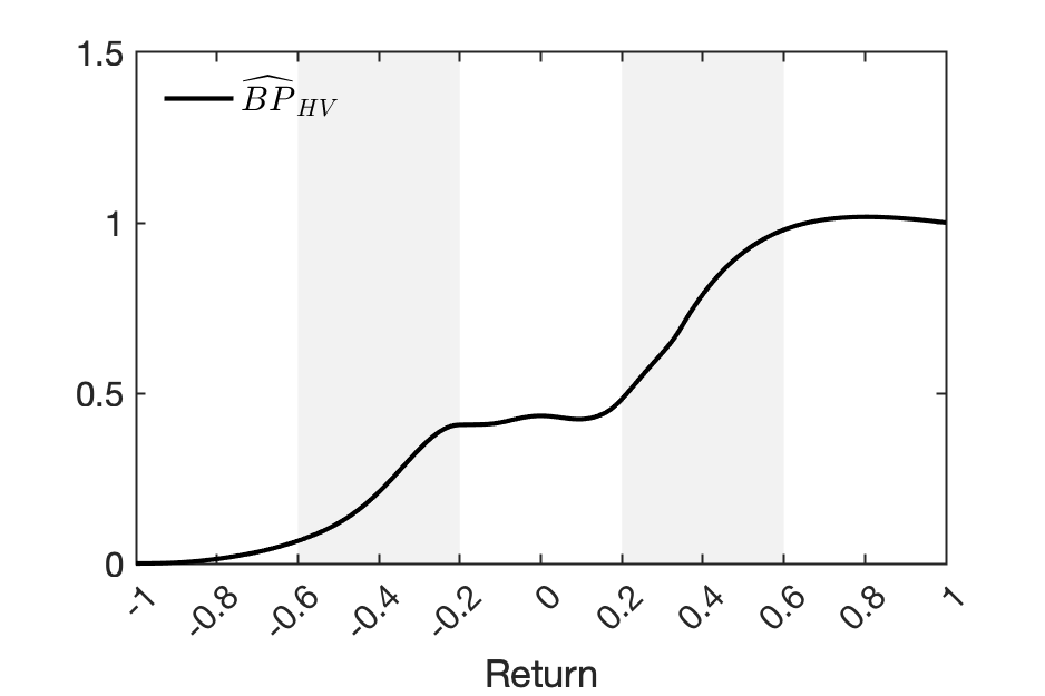
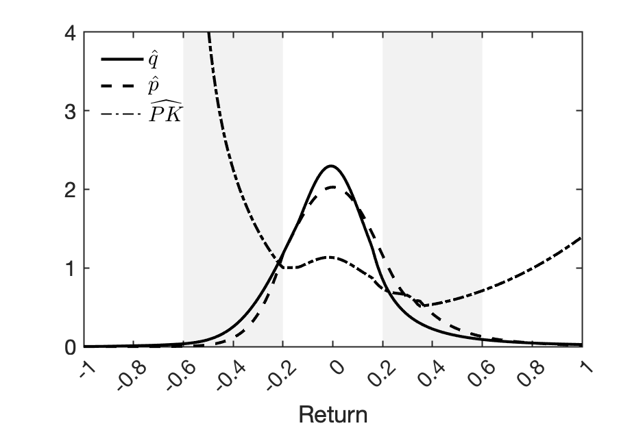
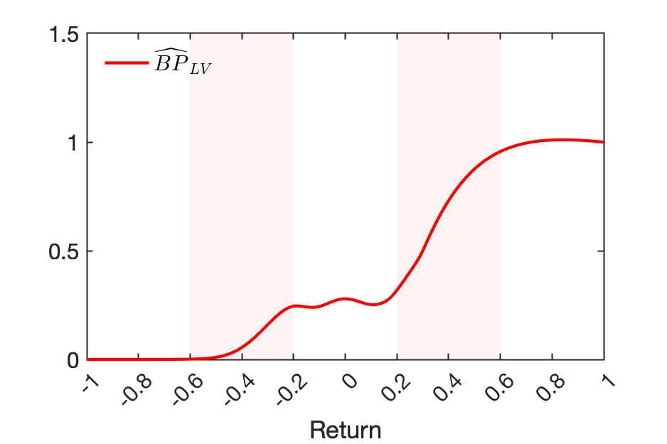
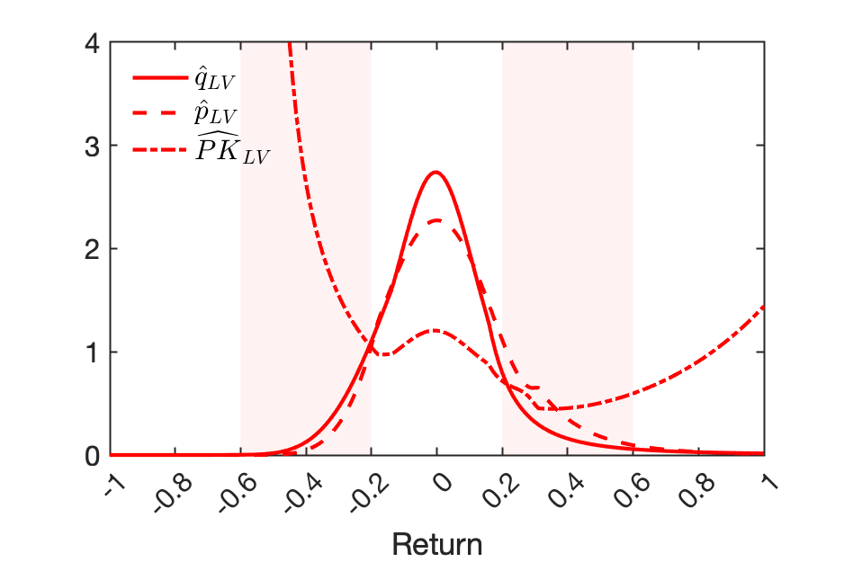
For the unconditional BP and PK estimates in Figure 1, we find that negative monthly returns between -60% and -20% and positive returns ranging from 20% - 60% account for 33.97% and 48.35%, respectively, to the Bitcoin premium. These features are interesting because they suggest that in the Bitcoin market, most of the contribution to the Bitcoin premium can be attributed to positive returns. The low contribution of the negative returns contrasts with the first moment premium for S&P 500 where (monthly) S&P 500 returns between -30% and -10% account for two-thirds of the equity premium reported by [12]. Next, we look closer into these functions across market regimes.

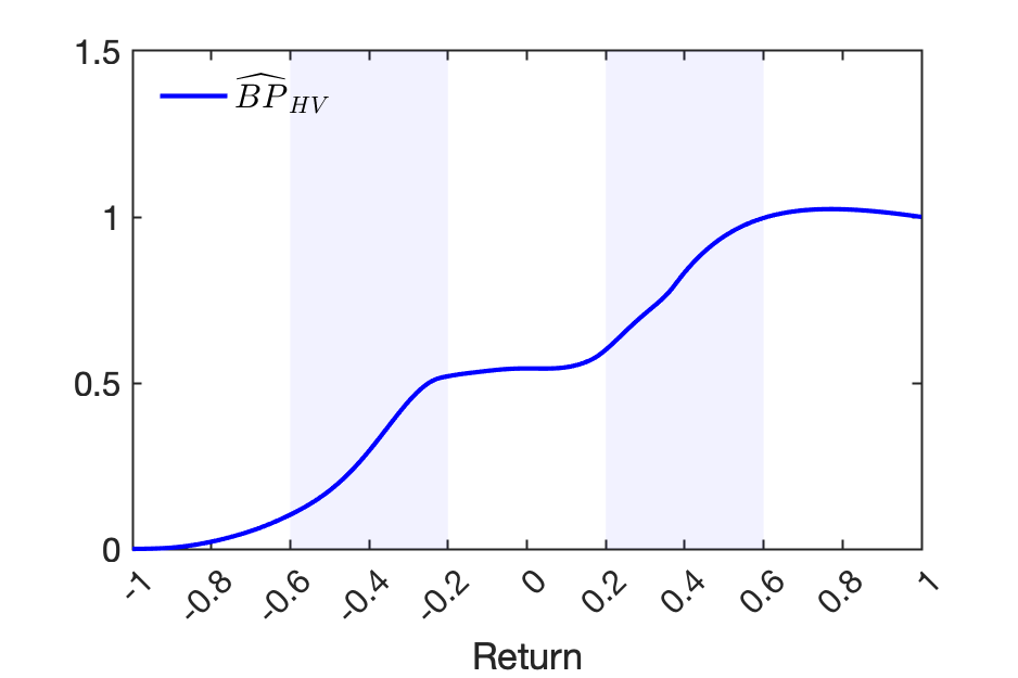
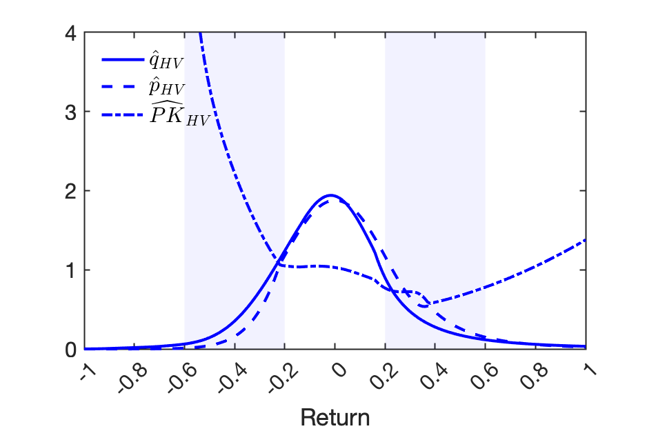
Figure 1 displays the BP function and the PK function for the two clusters, revealing several noteworthy characteristics. Notably, the shape of the HV cluster is more akin to the unconditional BP(x). But there are also some important differences. First, the high negative returns have a stronger impact on the BP(x), i.e., states of returns between -80% to -50% account for around 15% of the BP, indicating that investors are concerned about rare disasters. Secondly, the significance of positive returns is much reduced, with returns ranging from 20% to 60% contributing only 38.66% to the BP. The pricing kernel slope exhibits similarity in both the unconditional and high volatility regimes. There is a slight increment in the pricing kernel slope in the region of positive returns. The LV cluster, characterized by low volatility, exhibits a steeper increase in the region of positive returns. We identify a novel pattern of returns ranging from 20% to 60% that exhibits a significant 62.17% positive contribution to the BP. The negative returns from -60% to -20% only contribute 19.87% to the BP. The PK in LV regime, as well as in the unconditional and HV regime, consistently exhibits a U-shaped pattern. Across all three cases, the portion of PK being above 1 for returns above 0.6 corresponds to a slightly declining BP(x). Figure B2 offers an intuitive comparison of the PKs. Notbaly, the PK’s slope for negative returns is steeper in the LV cluster, suggesting a higher level of risk averson.

To better understand the relationship between BP and PK, we calculate the price of risk as the ratio of the average $\mathbb{Q}$ density to the $\mathbb{P}$ density, $\mathbb{E}_{\mathbb{Q}}(r)/\mathbb{E}_{\mathbb{P}}(r)$. Table 5 presents the BP contribution, physical probability, and price of risk for the intervals [-0.6, -0.2] and [0.2, 0.6], similar to Table 1 in [12]. For negative states, the price of risk for BTC is approximately 1.48, which is lower than the 2.63 for the S&P 500 as reported by [12], but comparable to levels found in [19], [10], [11], and [71].

Characteristics of BP, $\mathbb{Q}$ and $\mathbb{P}$ in influential states Negative states Positive states BP(-0.2)-BP(-0.6) $\int_{-0.6}^{-0.2}p(r)dr$ $\frac{\int_{-0.6}^{-0.2}q(r)dr}{\int_{-0.6}^{-0.2}p(r)dr}$ BP(0.2)-BP(0.6) $\int_{0.2}^{0.6}p(r)dr$ $\frac{\int_{0.2}^{0.6}q(r)dr}{\int_{0.2}^{0.6}p(r)dr}$ Overall 0.34 0.09 1.48 0.48 0.18 0.62 HV 0.42 0.11 1.53 0.39 0.19 0.69 LV 0.24 0.07 1.44 0.62 0.16 0.54 BP(-0.2)-BP(-0.6) and BP(0.2)-BP(0.6) are BP contributions on the intervals. $\int p(r)dr$ is the physical probability on such states and $\frac{\int q(r)dr}{\int p(r)dr}$ is the corresponding price of risk.

5.1 Discussion

The calibration of long-run risks and habit models to the S&P 500 index data in [12] suggests a symmetric contribution to the BP of positive and negative returns (each captures approximately 50% of the BP). However, the range of returns relevant for explaining the BP is confined to a tight interval of [-20%,  20%] monthly returns. These patterns suggest that the mean slope of the BP in both regions is approximately the same. In the case of BTC, this work shows that the positive returns contributing to the BP encompass a narrower range, in contrast to the negative returns that are more widely distributed. Simply put, the $\textrm{BP}(x)$ over the positive returns exhibit a higher slope, whereas it has a lower slope over the negative returns. This disparity implies that the long-term risks and habit models tend to overlook a crucial aspect of the crash. [71] combines the long-run risks and disaster mechanisms, but her model yields a too large contribution of the extreme events to the BP. This suggests that a different mechanism may be required to link the two models to explain the BTC market if one wants to build on long-run risk and habit models.

Relying on fully nonparametric estimates, we document an increase in risk aversion in the Bitcoin market in less volatile markets, as evidenced by a steeper slope of the pricing kernel over negative returns. This finding is consistent with [63] that negative returns are substantially more painful to investors in periods of low volatility. It is important to note, however, that while [63] employ a parametric specification of the pricing kernel, we use a fully nonparametric approach and still obtain the same results. Additionally, their study focuses on the negative returns side, whereas we examine the pricing kernel across the entire range of returns.

Our results align with those of [63] in terms of the direction of change of the PK slope as a function of volatility. However, our methodological approach is fundamentally different. Their approach involves selecting an exogenous variable to proxy for index volatility. They then perform a maximum likelihood estimation of a parametrically specified pricing kernel, which depends on the ex-ante chosen volatile. In contrast, our approach is fully nonparametric and does not involve the pre-selection of a conditioning variable. We interpret the clusters by investigating their drivers and find volatility to be instrumental. However, we acknowledge that the explanatory power of volatility in this regard is limited, as there may be other market forces at play. Therefore, our approach is more general. It is reassuring that two disparate methodological frameworks using different datasets lead to the same stylized facts. Our research corroborates the relationship between PK slopes (concavity) and volatility in both the S&P 500 index and the Bitcoin market.

6 Conclusion

This work uses marginal projections of the Pricing Kernel on the space of Bitcoin index returns to study Bitcoin risk premium properties. The Bitcoin index first moment premium and volatility risk premium are estimated from joint options and returns data over the most extensive period available. A Bitcoin Premium decomposition is applied as a function of returns. We also propose a new functional clustering method applied to a sequence of time-series of Bitcoin risk-neutral measures that allows us to obtain conditional measures for Bitcoin first moment and variance risk premia. Overall we find that, Bitcoin first moment, Variance risk Premia and premium for positive returns are all much larger than the corresponding measures for traditional assets like S&P500. Our findings for the Bitcoin BP decomposition can not be reconciled with any traditional macro-finance model, including habits ([19]), long-run risks model ([10]), rare disaster ([11]), and disappointment aversion ([62]).

[appendices] [appendices]l1

Appendices

Appendix A Main Appendix

A.1 Further Data Analysis

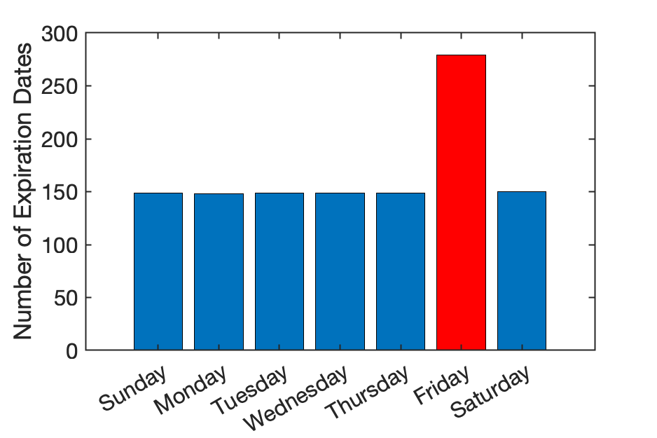
Two types of BTC options are traded on Deribit: those with shorter tenors that expire daily at 08:00 UTC and those with longer tenors that expire on Fridays at 08:00 UTC. Figure A1 presents the weekly distribution of expiration dates in our dataset for both types of options. Specifically, options with a TTM of two days or less expire on every day of the week, including Friday, while options with a TTM exceeding two days only expire on Fridays.

(a)

(b)

Figure A1: The weekly distribution of expiration dates in our dataset for (a) options with TTM of 2 days or less, and (b) options with TTM exceeding two days. The distribution spans from Sunday to Saturday, describing the frequency of option maturities across different days of the week.

(a)

(b)

Figure A2: The distribution of expiration dates across our dataset, for (a) all options, showcasing a range with the maximum TTM reaching up to 372 days; and (b) a subset of options with TTM no more than 64 days, providing an insight of the distribution patterns associated with shorter tenors.

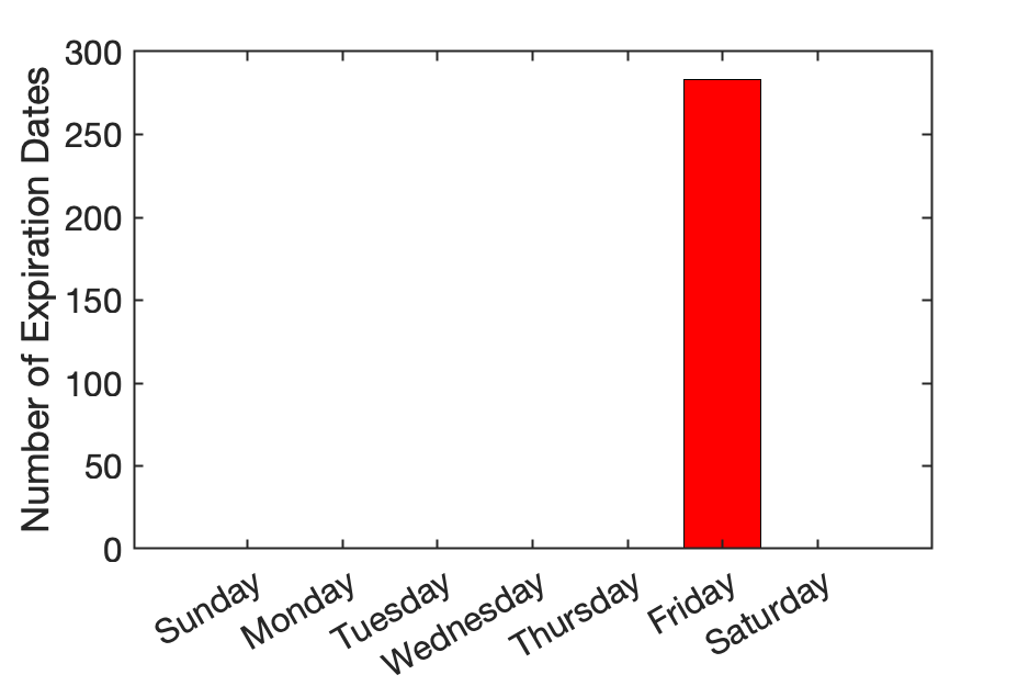
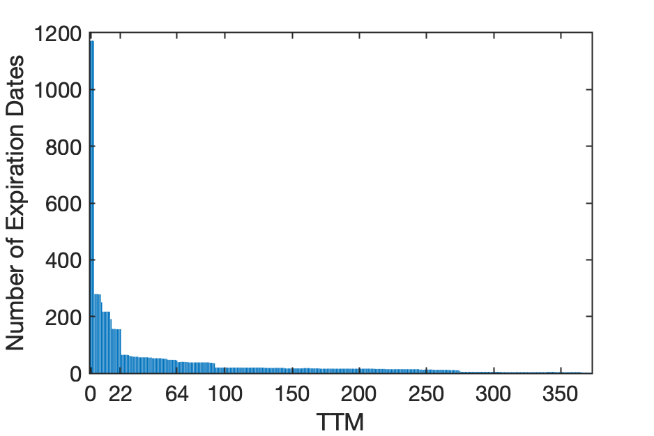
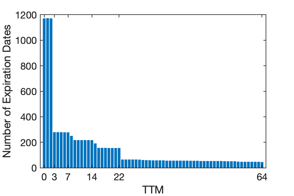
Additionally, it is important to note that options with varying TTMs might have distinct expiration dates. As the TTM diminishes to 0 for a given option, its expiration date remains constant. Figure A2 illustrates our dataset’s observed expiration dates for different TTMs. Options with TTMs shorter than three days exhibit a significantly higher number of expiration dates, corroborating that these options expire daily in contrast to others expire only on Fridays. Consequently, the variety of expiration dates tends to decrease as the TTM lengthens. For options with longer maturity, there is a noticeable scarcity in the number of expiration dates, indicating a lower trading volume. Figure A3 illustrates the average daily BTC option transactions per month.

Figure A3: Average daily BTC option transaction per month

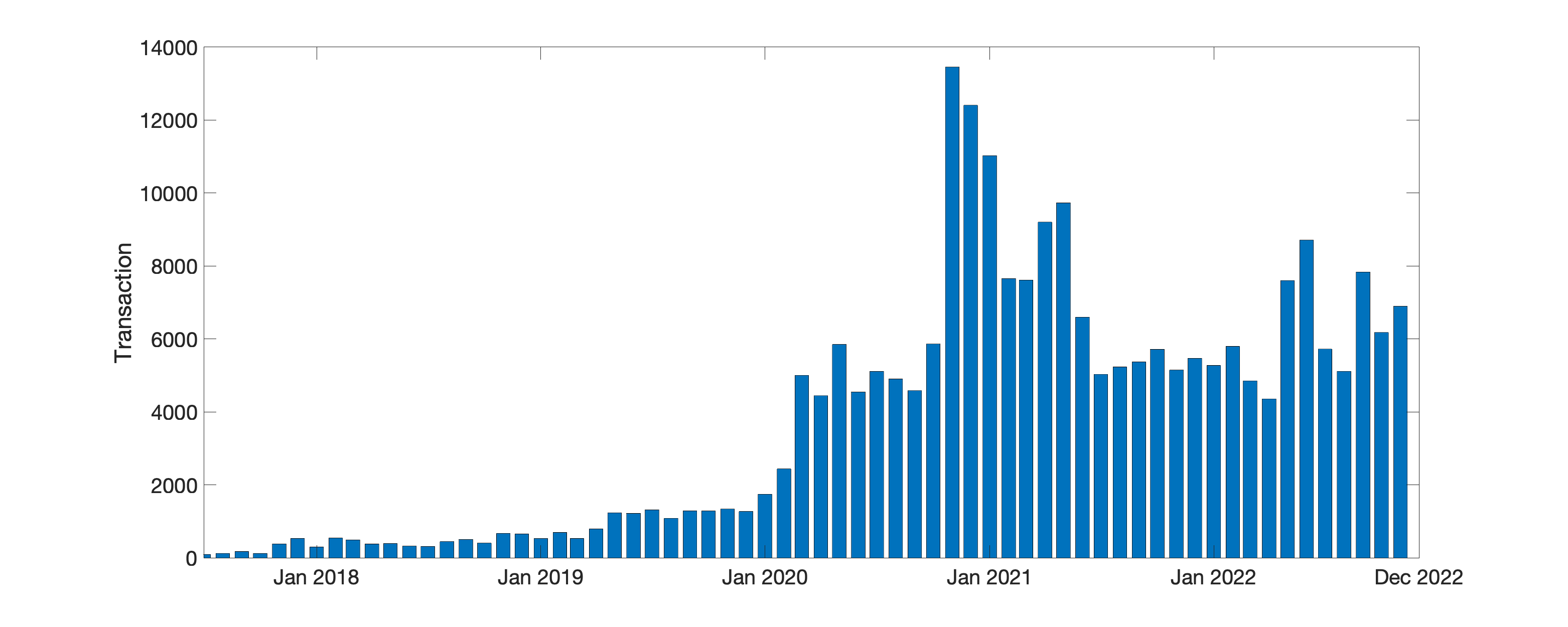Table A.1 gives an overview of the average implied volatility on different batches. We notice for both call and put options, IV initially decreases as moneyness increases and then rises past ATM, representing a "volatility smile" commonly seen in the traditional security markets. Furthermore, options with shorter maturity, particularly those deep OTM and deep ITM, tend to exhibit higher levels of IV. Notably, put options generally display higher IV compared to call options.

Implied volatility of BTC options [in level] Call options Moneyness (0, 9] [10, 26] [27, 33] >33 Average $(0,0.9)$ 1.31 1.05 0.92 0.92 1.07 $[0.9,0.97)$ 0.88 0.79 0.77 0.80 0.82 $[0.97,1.03]$ 0.70 0.73 0.73 0.78 0.81 $(1.03,1.1]$ 0.79 0.73 0.73 0.76 0.86 $>1.1$ 1.04 0.90 0.87 0.88 0.92 Average 0.81 0.82 0.83 0.86 0.82 Put options Moneyness (0, 9] [10, 26] [27, 33] >33 Average $(0,0.9)$ 1.25 1.03 0.97 0.94 1.05 $[0.9,0.97)$ 0.87 0.77 0.75 0.80 0.80 $[0.97,1.03]$ 0.70 0.74 0.74 0.80 0.78 $(1.03,1.1]$ 0.88 0.79 0.76 0.80 1.00 $>1.1$ 1.69 1.17 0.89 0.93 1.19 Average 0.89 0.90 0.88 0.90 0.89 This table presents the average implied volatility for the BTC option over moneyness and maturity. The columns are categorized based on the time to maturity in days. The IVs are calculated and listed by Deribit.

Table A.1 presents the transaction patterns of call and put options, classified into different moneyness and maturity groups. The results reveal that OTM options are predominant for both call and put options, accounting for more than 60% of the total, with deep OTM options making up more than 35%. In contrast, in-the-money (ITM) options constitute less than 10%, with deep ITM options accounting for less than 4%. Regarding the term structure, more than half of the options have maturities of less than 10 days, with a slightly higher proportion of put options (54.43%) compared to call options (51.12%). Moreover, call options with maturities of more than 33 days constitute 24.05%, whereas put options with maturities of more than 33 days account for 20.10%.

Summary statistics on transaction contracts of BTC options [in %] Call options Moneyness (0, 9] [10, 26] [27, 33] >33 Subtotal $(0,0.9)$ 0.99 0.55 0.19 1.42 3.15 $[0.9,0.97)$ 2.99 0.85 0.19 0.86 4.89 $[0.97,1.03]$ 22.50 3.93 0.53 1.77 28.74 $(1.03,1.1]$ 16.67 5.00 0.70 2.29 24.65 $>1.1$ 7.97 10.48 2.41 17.71 38.57 Total 51.12 20.81 4.02 24.05 100.00 Put options $(0,0.9)$ 10.38 10.53 2.11 12.83 35.84 $[0.9,0.97)$ 18.44 5.41 0.72 2.64 27.22 $[0.97,1.03]$ 22.54 4.16 0.49 1.97 29.16 $(1.03,1.1]$ 2.10 0.90 0.17 1.07 4.25 $>1.1$ 0.97 0.80 0.17 1.59 3.53 Total 54.43 21.80 3.66 20.10 100.00 This table presents the proportion of traded BTC option contracts over moneyness and maturity. The sample covers transactions between July 1, 2017 and December 17, 2022. The columns are categorized based on the time to maturity in days. The transactions are measured as the number of traded contracts.

Table A.1 provides summary statistics on option transaction quantity in BTC units, given that each option is denominated in BTC. The distribution of transaction quantity closely mirrors that of transaction contracts, with an even greater proportion of out-of-the-money options. Table A.1 presents the summary statistics on option transaction volume in USD, calculated as the traded quantity multiplied by the BTC price in USD. Options with longer maturities and in-the-money options typically possess higher values, resulting in over half of the total value being attributed to long-maturity options. Additionally, the OTM value portion is lower than transaction and volume due to their lower values.

Summary statistics on BTC option quantity [in %] Call options Moneyness (0, 9] [10, 26] [27, 33] >33 Subtotal $(0.00,0.90)$ 0.46 0.37 0.11 0.90 1.85 $[0.90,0.97)$ 1.55 0.63 0.18 0.66 3.03 $[0.97,1.03]$ 17.21 3.71 0.51 1.53 22.94 $(1.03,1.10]$ 16.14 6.17 0.82 2.30 25.43 $>1.1$ 8.84 13.10 3.45 21.37 46.75 Total 44.19 23.98 5.07 26.75 100.00 Put options $(0.00,0.90)$ 13.21 13.35 2.83 13.87 43.26 $[0.90,0.97)$ 17.83 6.73 0.85 2.48 27.89 $[0.97,1.03]$ 18.12 4.14 0.53 1.52 24.31 $(1.03,1.10]$ 1.11 0.57 0.11 0.70 2.49 $>1.1$ 0.47 0.56 0.08 0.94 2.05 Total 50.74 25.35 4.40 19.51 100.00 This table presents the proportion of quantity [in %] of the BTC option data over moneyness and maturity. The data spans from July 1, 2017, to December 17, 2022. The columns are categorized based on the time to maturity in days. The quantity is measured in terms of the number of BTC units.

Summary statistics on BTC option transaction volume valued in USD [in %] Call options Moneyness (0, 9] [10, 26] [27, 33] >33 Subtotal $(0.00,0.90)$ 2.01 2.72 0.56 9.15 14.45 $[0.90,0.97)$ 2.38 1.74 0.58 3.09 7.79 $[0.97,1.03]$ 8.53 6.11 1.07 5.04 20.74 $(1.03,1.10]$ 4.52 6.02 1.21 6.17 17.92 $>1.1$ 1.30 6.21 2.20 29.39 39.10 Total 44.19 22.81 5.61 52.84 100.00 Put options Moneyness (0, 9] [10, 26] [27, 33] >33 Subtotal $(0.00,0.90)$  5.37 5.37 1.50 16.69 25.40 $[0.90,0.97)$  6.30 6.30 1.14 6.98 19.79 $[0.97,1.03]$  9.85 6.32 1.00 5.59 22.76 $(1.03,1.10]$  2.08 1.52 0.33 3.59 7.53 $>1.1$  2.88 3.46 0.69 17.48 24.51 Total 22.01 22.98 4.67 50.34 100.00 This table presents summary statistics for the volume of BTC options. The volume is measured in USD, i.e., volume = quantity $\times$ BTC price (USD) summed in each category. The data spans from July 1, 2017, to December 17, 2022. The columns are categorized based on the time to maturity in days. Within each moneyness and maturity category, the entries provide the volume proportions in percentage.

A.2 Estimation of the BVIX

The BVIX is calculated using the BTC transaction data as described in Section 2. We calculate the variances $\sigma_{1}^{2}$ and $\sigma_{2}^{2}$ by closely following the original VIX methodology of CBOE and interpolate the time-weighted average as

$$\operatorname{BVIX}_{\tau}=100\times\sqrt{\left\{N_{T_{1}}\sigma_{1}^{2}\left[\frac{N_{T_{2}}-\frac{\tau}{365}}{N_{T_{2}}-N_{T_{1}}}\right]+N_{T_{2}}\sigma_{2}^{2}\left[\frac{\frac{\tau}{365}-N_{T_{1}}}{N_{T_{2}}-N_{T_{1}}}\right]\right\}\times\frac{365}{\tau}},$$ (27)

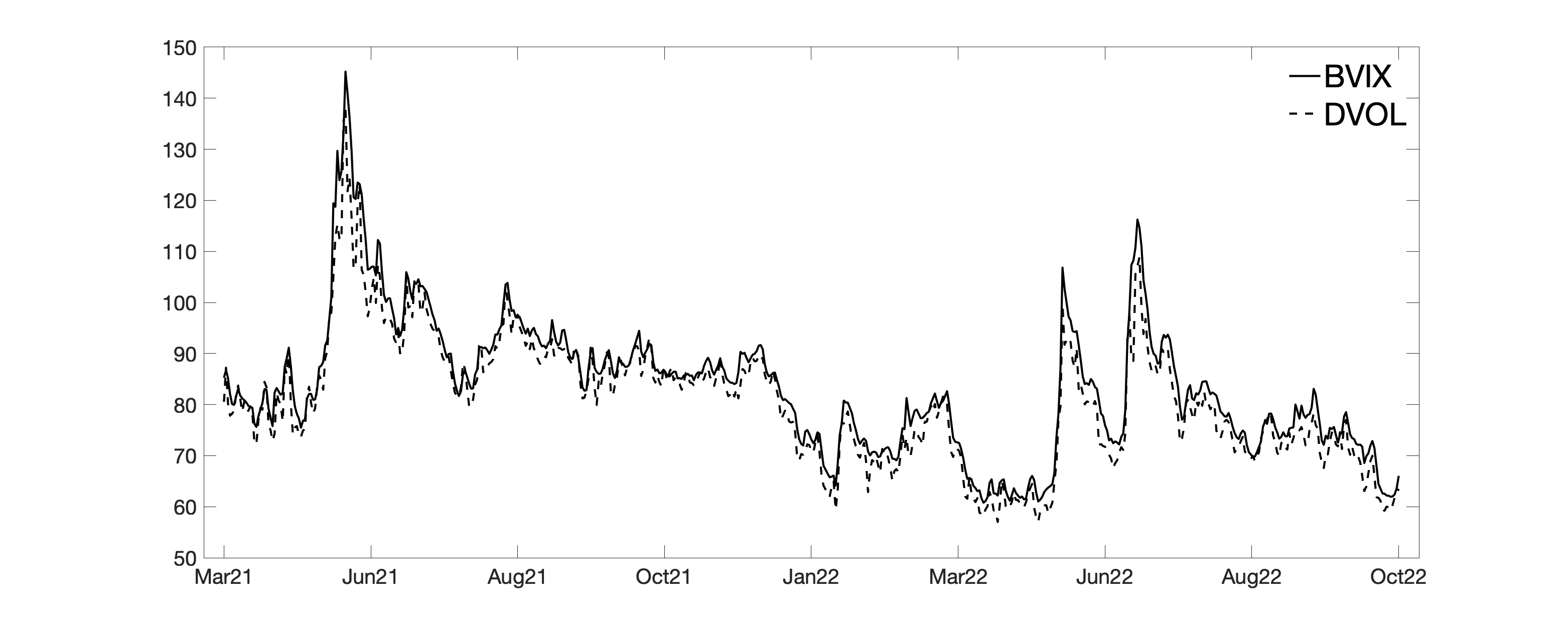
where $N_{T_{1}}=\frac{T_{1}}{365}$ and $N_{T_{2}}=\frac{T_{2}}{365}$ is the time to settlement (in years) of the near and next-term options, respectively. A comparison of the BVIX to the Dvol index by Deribit is conducted in Figure A4. As we see, both indices are closely related.

Figure A4: BVIX vs. Deribit Dvol Index

A.3 Interpolation of the IV Surface

The SVI model is widely popularized due to its parametric specification as well as good performance in the interpolation of IVs. Additionally assuming linearity in $\tau$ allows a more flexible representation of the implied volatility surface, providing a better fit to data by allowing each parameter to exhibit its term structure.

We are using the IV of each transaction given by the Deribit exchange, as described in Section 2. After applying local polynomial estimation, we obtain a smooth curve of IV for a given day as a function of moneyness. The parameters are linear functions of $\tau$ and capture various characteristics of the volatility smile such as its level, slope, and curvature. More specifically, the parameters are denoted as $a(\tau)=\alpha_{0}+\alpha_{1}\cdot\tau,\ b(\tau)=\beta_{0}+\beta_{1}\cdot\tau,\ \rho(\tau)=\rho_{0}+\rho_{1}\cdot\tau,\ m(\tau)=m_{0}+m_{1}\cdot\tau$ and $\sigma(\tau)=\sigma_{0}+\sigma_{1}\cdot\tau$. The parameter vector $\theta=[\alpha_{0},\beta_{0},\rho_{0},m_{0},\sigma_{0},\alpha_{1},\beta_{1},\rho_{1},m_{1},\sigma_{1}]$ is estimated by minimizing the root mean squared error (RMSE)

$$\hat{\theta}_{t}=\underset{\theta}{\arg\min}\sqrt{\frac{1}{N_{t}}\sum_{i=1}^{N_{t}}\left\{\omega_{t,i}-\omega\left(r_{t,i},\tau_{t,i};\theta\right)\right\}^{2}},$$

where $\omega_{t,i}$ is the (squared) observed IV and $\omega\left(r_{t,i},\tau_{t,i};\theta\right)$ is the implied variance as defined in Equation 8 for day $t$ and corresponding transaction $i$.

Figure A5: First row: Average IV surface interpolated by SVI for the HV cluster (left) and LV cluster (right). The black curve within each panel is the IV for TTM 27 days. Second row: Risk-neutral densities for the HV (left) and LV (right) cluster. The solid curve is the average risk-neutral density for the respective cluster.

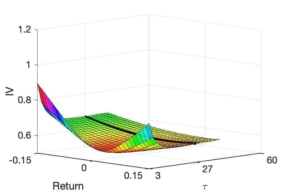
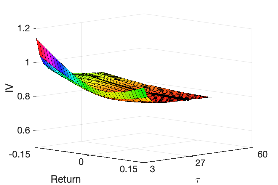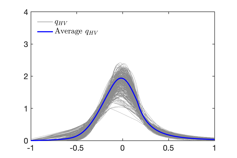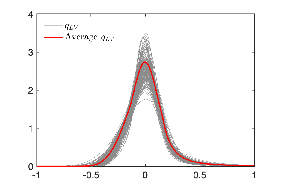A.4 Estimation of Parametric Tails

Inspired by [34], we use the Generalized Extrem Value (GEV) distribution to fit the tails of the risk-neutral density. Acknowledging the fact that transaction limits truncate the density at both lower and upper extremes, we address the concern that this truncation neglects trading at deeply in-the-money and deeply out-of-the-money options. To rectify this, our objective is to construct a density with extended tails that captures these extreme areas. It covers the full return support and satisfies essential moment conditions. For example, the integration of the density has to equal to one and the first moment of the density has to align with the assumed risk-free rate.

We use the GEV distribution to fit both, the left and the right tail. However, we deviate from [34] in two aspects due to the special nature of the BTC data, the target points selection and the moment conditions.

In order to fit the GEV distribution, [34] fixes so-called target points. Hereby, the author initially fixes the 0.02, 0.05, 0.95, and 0.98 quantiles of the cumulative distribution function $F(x)$ for the tail estimation, i.e. $r_{1}=F^{-1}_{r}(0.02)$, $r_{2}=F^{-1}_{r}(0.05)$ for the left tail and $r_{3}=F^{-1}_{r}(0.05)$, $r_{4}=F^{-1}_{r}(0.98)$ for the right tail. However, BTC option data has peculiar characteristics and often lacks adequate extremity coverage. Thus, we select two target points per tail that are closest to 0.02 and 0.05 for the left tail, and 0.95 and 0.98 for the right tail. This procedure ensures data representativeness within the constraints of the available information.

The second deviation lies in the moment constraints. We enforce the synthetic densities to ensure that the integral over each density is equal one. In addition, we align the first moment of the risk-neutral density with the risk-free rate $R^{f}$.

First, let us defined the target points on the left tail as $r_{1},r_{2}$,

$$\left\{\begin{aligned} &r_{1}=\mathbb{Q}^{-1}\left(0.02\right),r_{2}=\mathbb{Q}^{-1}(0.05),&&\text{if}\;\min\mathbb{Q}<0.02,\\ &r_{1}=\mathbb{Q}^{-1}\left(\min\mathbb{Q}\right),r_{2}=\mathbb{Q}^{-1}\left(\min\mathbb{Q}+0.03\right),&&\text{if}\;\min\mathbb{Q}\geq 0.02,\end{aligned}\right.$$

and the target points on the right tail as $r_{3},r_{4}$,

$$\left\{\begin{aligned} &r_{3}=\mathbb{Q}^{-1}(0.95),r_{4}=\mathbb{Q}^{-1}\left(0.98\right),&&\text{if}\;\max\mathbb{Q}>0.98,\\ &r_{3}=\mathbb{Q}^{-1}\left(\max\mathbb{Q}-0.03\right),r_{4}=\mathbb{Q}^{-1}\left(\max\mathbb{Q}\right),&&\text{if}\;\max\mathbb{Q}\leq 0.98.\end{aligned}\right.$$

For a given risk-neutral density $q_{t}(R)=q(R)$, the parameters of the GEV distribution for both tails, i.e. $\theta=(\xi_{l},a_{l},b_{l},\xi_{r},a_{r},b_{r})$, are estimated by solving the following minimization problem

$$\hat{\theta}=\arg\min_{\theta} \sum_{i=1}^{2}\left\|q(r_{i})-f_{GEV}(r_{i};\xi_{l},a_{l},b_{l})\right\|^{2}+\left\|q(r_{1})-F_{GEV}(r_{1};\xi_{l},a_{l},b_{l})\right\|^{2}$$

$$+\sum_{i=3}^{4}\left\|q(r_{i})-f_{GEV}(r_{i};\xi_{r},a_{r},b_{r})\right\|^{2}+\left\|q(r_{1})-F_{GEV}(r_{1};\xi_{r},a_{r},b_{r})\right\|^{2}$$

$$s.t. \left\{\begin{aligned} &q(r_{1})=f_{GEV}(r_{1};\xi_{l},a_{l},b_{l})\\ &q(r_{1})=F_{GEV}(r_{1};\xi_{l},a_{l},b_{l})\\ &q(r_{4})=f_{GEV}(r_{4};\xi_{r},a_{r},b_{r})\\ &q(r_{4})=F_{GEV}(r_{4};\xi_{r},a_{r},b_{r})\\ &\int_{-\infty}^{r_{1}}f_{GEV}(r;\xi_{l},a_{l},b_{l})dr+\int_{r_{1}}^{r_{4}}q(r)dr+\int_{r_{4}}^{\infty}f_{GEV}(r;\xi_{r},a_{r},b_{r})dr=R_{f}\times\frac{\tau}{365},\\ \end{aligned}\right.$$

where $R_{f}$ is risk-free rate, and $\tau$ is time to maturity.

A.5 Bitcoin Premium

Figure A6: BP across different number of bins (NB) using empirical PDF for the $\mathbb{P}$ density with TTM 27 days.

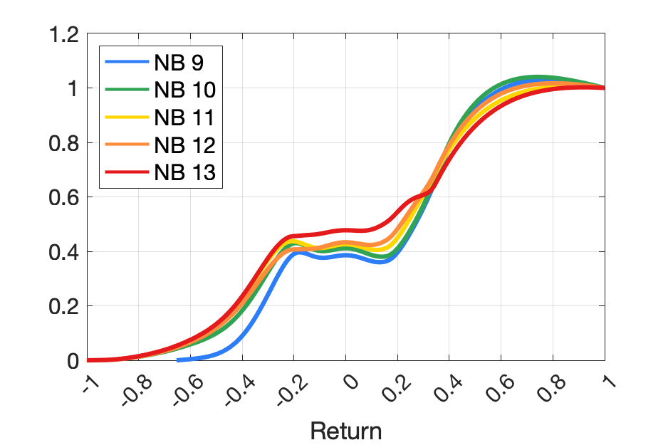
In the estimation of empirical PDF, as $\mathbb{P}$ density, the selection of the smoothing parameter, i.e. the number of equally distant bins, can influence the shape of $\mathbb{P}$. Consequently, this affects the shape of BP. To demonstrate the robustness of BP across various smoothing parameters, Figure A6 shows the robustness of BP with different number of bins (NB). In the main text of the paper, we use NB of 11. Despite variations in NB, the basic shape of BP remains relatively consistent.

A.6 Dimensionality Reduction and Clusters

The UMAP (Uniform Manifold Approximation and Projection) is a nonlinear dimensionality reduction technique, recently proposed by [54]. It builds a topological representation of the high dimensional data set and then minimizes the following cross entropy loss function

$$\sum_{e\in E}w_{h}(e)\log\left(\frac{w_{h}(e)}{w_{l}(e)}\right)+\left(1-w_{h}(e)\right)\log\left(\frac{1-w_{h}(e)}{1-w_{l}(e)}\right),$$ (28)

where $w_{h}(e)$ is the weight of the 1-simplex $e$ in the high dimensional case and $w_{l}(e)$ is the weight of $e$ in the low dimensional case. The set of all possible 1-simplices is represented as $E$. It has been designed to preserve the local as well as the global structure of the data. The result is illustrated in Figure 7(b). Further, we illustrate the first two principal components of the distance matrix in Figure 7(a).

(a)

(b)

Figure A7: (a) First two principal components of the Euclidean distance matrix of risk-neutral densities. (b) Three dimensional UMAP of risk-neutral densities. Blue is the HV cluster and red is the LV cluster. Both figures refer to the multivariate risk-neutral density composition.

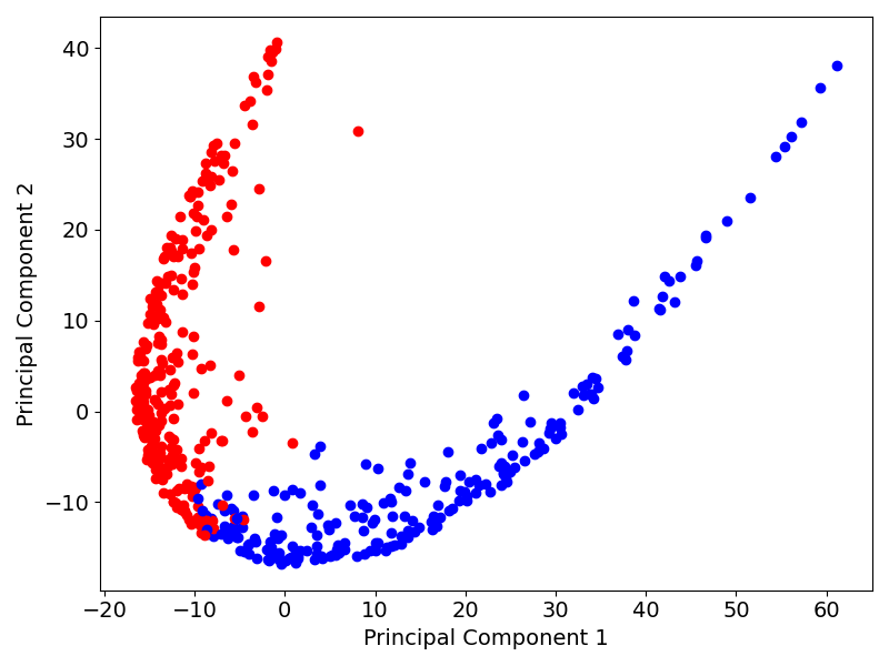
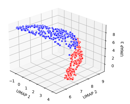
Appendix B Miscellaneous

This appendix includes miscellaneous results to support our empirical arguments, especially providing further robustness checks. It can also be seen as a starting point for further research.

B.1 Further Cluster Analysis

Figure B1 provides another way to view $\mathbb{Q}$-density in HV and LV clusters for different time-to-maturity. This figure indicates that the clusters are consistent for different TTMs and underlines the multivariate clustering approach.

Table B.1 shows the average realized returns (RR) and future returns (FR) on the clustering dates, where returns are simple returns. This indicates that the LV cluster has higher RR, and the HV cluster has higher FR. Table B.1 displays the logistic regression of the clusters on BP, BVIX, and VRP. It reveals that BP calculated by realized return minus risk-free rate can not explain the cluster variation. BVIX shows substantial explainable power, accounting for nearly half of the cluster variance. VRP calculated by $q$ variance minus realized variance is not significant. The coefficients indicate that a higher BVIX index is associated with a higher probability of HV cluster, i.e., the high volatility cluster. Table B.1 displays the logistic regression examining the relationship between the clusters and the first four moments of risk-neutral density. The variance explains 69% of the variation in clusters on its own. When combined, all four moments together account for 70% of the cluster variation. Table B1 presents the logistic regression of clusters with single factors using time-to-maturity 27 days. The dependent variable is the cluster label, while the independent variables include realized returns (RR), realized variance (RV), BVIX, $\mathbb{Q}$ variance, VRP(calculated either by BVIX or RV), jumps (including negative and positive jumps) and sentiment index. Significant factors include RR, RV, BVIX, $\mathbb{Q}$ variance, and negative and positive jumps separately. Only RV, BVIX, and $\mathbb{Q}$ variance have good explanation power. Figure B2 compares the Bitcoin premium and pricing kernel for overall (OA), high-volatility cluster (HV) and low-volatility cluster (LV). Figure B3 displays the distribution of daily average BTC option transactions, categorized by clusters and also differentiated into call and put options. This visual illustration confirms that most transactions are OTM for both call and put options, aligning with the summary statistics of transactions we showed in Table A.1. Regarding the clustering aspect, the figure indicates that cluster 0 typically experiences higher daily average transactions than cluster 1.

Figure B1: Risk-neutral densities term structures viewed from the side. From the first row to the fourth row, the time to maturity is 5, 9, 14, and 27 days, respectively. The HV cluster is colored in blue and the LV cluster is colored in red.

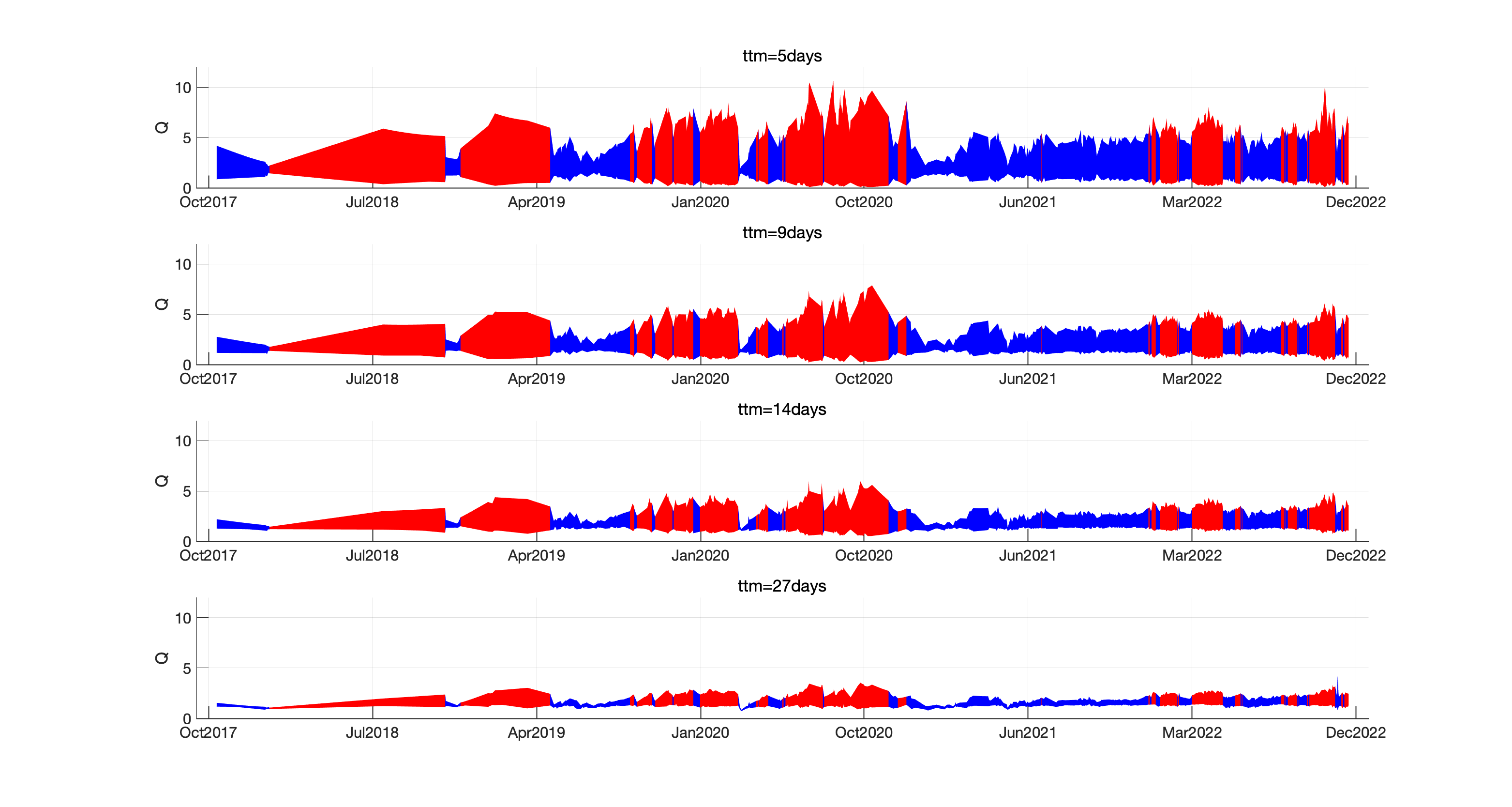Average realized returns (RR) and future returns (FR) on the clustering dates Overall HV LV RR (%) 5.64 0.41 12.05 FR (%) 10.27 53.83 -43.09 Num 505 278 227 On each date, we calculate the 27-day realized return (RR) and future return (FR). We report the average RR and FR for each cluster. In comparison, the average 27-day return from Jan 1, 2014 to Dec 31, 2022 is 67.93%, and the average 27-day return from Jan 1, 2015 to Dec 31, 2022 is 53.34%. RR and FR are annualized simple returns.

Logistic Regression of Clusters on BP, BVIX, and VRP (1) (2) (3) (4) (5) Constant -0.20[**] -1.21[***] -0.25[***] -1.21[***] -0.25[***] (0.09) (0.18) (0.09) (0.18) (0.09) BP 0.12 -0.25 0.11[***] (0.09) (0.18) (0.10) BVIX -3.75[***] -5.37 (0.33) (0.34) VRP 0.15 0.12 (0.11) (0.11) R2 0.00 0.49 0.00 0.50 0.01 Adj. R2 -0.00 0.45 0.00 0.49 0.00 $T_{HV}$ 278 271 271 271 271 $T_{LV}$ 227 211 211 211 211 $T$ 505 482 482 482 482 This table displays the logistic regression of the clusters on BP, BVIX, and VRP. The dependent variable is the cluster label. The independent variables are BP, BVIX, and VRP. The number of observations in the HV cluster, LV cluster, and the overall sample is denoted as $T_{HV}$, $T_{LV}$ and $T$, respectively. It reveals that BP calculated by realized return minus risk-free rate can not explain the cluster variation. BVIX shows substantial explainable power, accounting for nearly half of the cluster variance. VRP calculated by $q$ variance minus realized variance is not significant. The coefficients indicate that a higher BVIX index is associated with a higher probability of HV cluster, i.e., the high volatility cluster.

Logistic Regression of clusters on first four moments (1) (2) (3) (4) (5) Constant -0.43*** -2.50*** -0.46*** -0.18 -2.19*** (0.11) (0.33) (0.11) (0.15) (0.65) Mean 1.55*** 0.30 (0.21) (0.40) Variance -7.70*** -6.28*** (0.80) (1.78) Skewness 1.85*** -0.04 (0.20) (0.74) Kurtosis 3.93*** 1.04 (0.36) (1.50) R2 0.14 0.69 0.24 0.60 0.70 This table displays the logistic regression examining the relationship between the clusters and the first four moments of risk-neutral density. The dependent variable is the cluster label, and the independent variables include annualized mean, annualized variance, skewness, and excess kurtosis of risk-neutral density. All four moments are standardized. The number of observations in the high-volatility (HV) cluster, low-volatility (LV) cluster, and the overall sample is $T_{HV}=278$, $T_{LV}=227$ and $T=505$, respectively. The variance explains 69% of the variation in clusters on its own. When combined, all four moments together account for 70% of the cluster variation.

Table B1: Logistic regression of clusters, with single factors TTM=27

	(1)	(2)	(3)	(4)	(5)	(6)	(7)	(8)	(9)	(10)
Constant	-0.20**	-1.08***	-1.22***	-2.50***	-0.25***	-0.25***	-0.20**	-0.24***	-0.23**	-0.20***
	(0.09)	(0.17)	(0.181)	(0.33)	(0.09)	(0.09)	(0.09)	(0.09)	(0.09)	(0.09)
RR	0.15*
	(0.09)
RV		-3.90***
		(0.41)
BVIX			-3.75***
			(0.33)
$\mathbb{Q}$ variance				-7.70***
VRP(BVIX)					0.15
					(0.11)
VRP(RV)						0.15
						(0.11)
Jump							0.07
							(0.45)
Jump(-)								0.60***
								(0.18)
Jump(+)									-0.48***
									(0.16)
Sentix										0.02
										(0.09)
R2	0.00	0.28	0.49	0.69	0.00	0.00	0.00	0.02	0.02	0.00
Num. Cluster 0	278	271	271	278	271	271	278	278	278	278
Num. Cluster 1	227	211	211	227	211	211	227	227	227	227
Num. Total	505	482	482	505	482	482	505	505	505	505

(a)

(b)

Figure B2: (a) BP during high volatility (HV) regime in blue, during low volatility (LV) regime in red, and during both clusters overall (OA) in black. (b) PK during the high volatility (HV) regime in blue, during the low volatility (LV) regime in red, and during both clusters overall (OA) in black. The cluster-specific estimates utilize cluster-specific empirical densities: $q_{i}$ density is estimated as the average of daily estimated densities belonging to the respective cluster; $p_{i}$ density is estimated by rescaled (by the cluster-specific empirical volatility) empirical PDF of the full sample overlapping returns, for $i\in\{\text{HV},\text{LV}\}$.

Figure B3: Daily average transaction distribution for different clusters and for call and put, respectively.

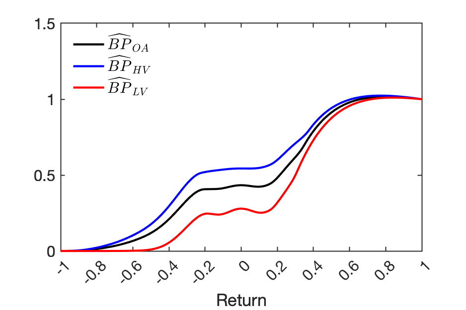
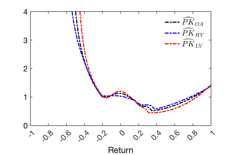
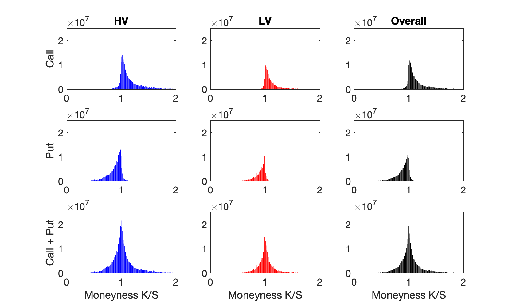
B.2 Time-varying BP and VRP

(a)

(b)

Figure B4: Lower bounds of BP and estimates of VRP over time. (a) The calculation of lower bounds follows the methodologies of [53] and [23], but is based on our estimated risk-neutral density $\hat{q}_{t}$. Parameters are estimated using a two-step nonlinear least squares method, with the gross return set to 1 to align with the BTC risk-free rate. The average lower bounds calculated using the three methods are 60.85%, 65.32%, and 68.05%, respectively. (b) $\textrm{VRP}_{t}$ is calculated as the difference between $\text{BVIX}_{t}^{2}$ and $\textrm{RV}_{t}$, consistent with the VRP presented on the right of Table 5 Panel B. $\textrm{VRP}_{t}$ estimates less than -2 are excluded, and the corresponding days are highlighted with shaded areas. Trends are illustrated using linear and LOESS (locally estimated scatterplot smoothing) fits in black and blue, respectively, with 95% confidence intervals estimated from 10,000 bootstrap samples.

(a)

(b)

Figure B5: BTC index, $\text{BVIX}^{2}$ and RV over time. Generally, $\text{BVIX}^{2}_{t}$ remains above $\textrm{RV}_{t}$, except for the dramatical period between Mar 15, 2020 and April 8, 2020 when RV approached 500% as BTC index surprisingly fell from $10,000 to $5,000 and rebounded within nearly two month.

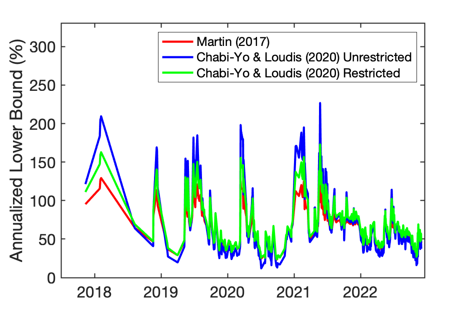
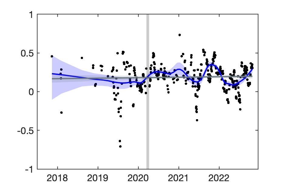
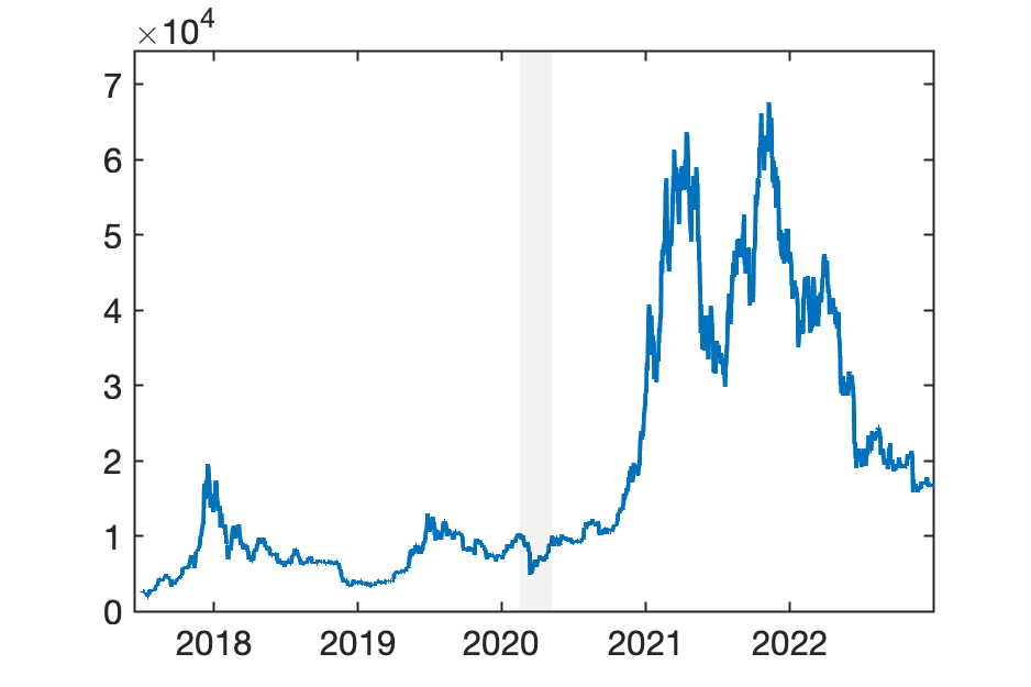
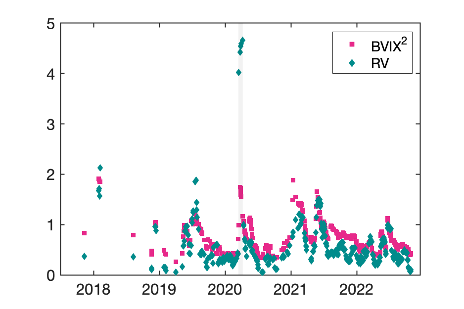
B.3 Robustness: VRP

In the above Section 5, we show VRP over time in Figure B4, employing $\mathbb{Q}$-variance based on the squared BVIX and $\mathbb{P}$-variance based on the realized variance. To provide more comprehensive VRPs, we provide alternatives of $\mathbb{Q}$-variance and $\mathbb{P}$-variance. For the robustness check of $\mathbb{P}$-variance, we use the second moment of $\mathbb{P}$ density estimated by empirical PDF and present VRP in Table B.3. Figure B6 presents two measures of VRP over time; the left is based on the empirical risk-neutral variance, and the right is based on BVIX.

(a)

(b)

Figure B6: VRP over time. In a) VRP is calculated by the second moment of empirical risk-neutral density minus RV. In b) VRP is calculated by BVIX minus RV.

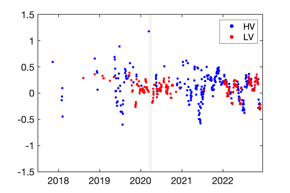
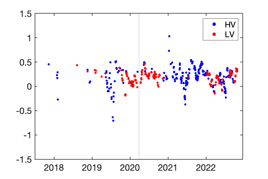
Robustness check: Risk Premia Based on $\mathbb{Q}$ density Based on BVIX Overall HV LV Overall HV LV $\mathrm{Var}_{\mathbb{Q}}(R)$ 0.63 0.80[***] 0.43[***] 0.71 0.88[***] 0.50[***] $\mathrm{Var}_{\mathbb{P}}(R)$ 0.68 0.71 0.32 0.68 0.71 0.32 VRP -0.04 0.09[***] 0.11[***] 0.04 0.16[***] 0.18[***] Observations 505 278 227 482 271 211 $\mathrm{Var}_{\mathbb{P}}(R)$ is $\sigma_{p}^{2}$.

B.4 Cost of Carry

Figure B7 shows the cost of carry, calculated using BTC futures data from [49], compared with the first moment of our estimated $\mathbb{Q}$ density.

Figure B7: Cost of carry, calculated using BTC futures data from [49], compared with the first moment of our estimated $\mathbb{Q}$ density

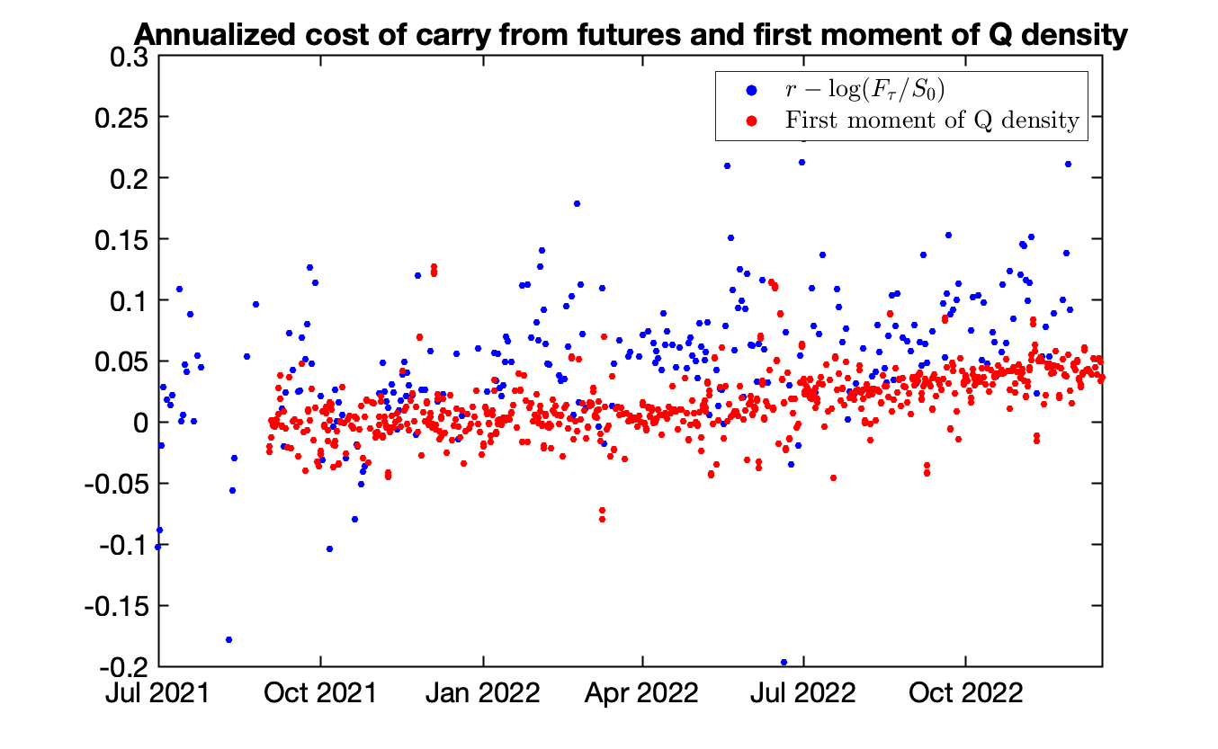
B.5 Further discussion about BP

Table B.5 show characteristics of BP, $\mathbb{Q}$ and $\mathbb{P}$ in influential states, similar to the Table 1 in [12] paper, and Table B.5 provide another measure of risk price.

Characteristics of BP, $\mathbb{Q}$ and $\mathbb{P}$ in influential states Panel A: Separate cluster analysis BP Negative states Positive states BP(-0.2)-BP(-0.6) $\int_{-0.6}^{-0.2}p(r)dr$ $\frac{\int_{-0.6}^{-0.2}q(r)dr}{\int_{-0.6}^{-0.2}p(r)dr}$ BP(0.2)-BP(0.6) $\int_{0.2}^{0.6}p(r)dr$ $\frac{\int_{0.2}^{0.6}q(r)dr}{\int_{0.2}^{0.6}p(r)dr}$ Overall 0.34 0.09 1.48 0.48 0.178 0.62 HV 0.42 0.11 1.53 0.39 0.19 0.69 LV 0.24 0.07 1.44 0.62 0.16 0.54 Panel B: Decomposition cluster analysis BP Negative states Positive states BP(-0.2)-BP(-0.6) $\int_{-0.6}^{-0.2}p(r)dr$ $\frac{\int_{-0.6}^{-0.2}q(r)dr}{\int_{-0.6}^{-0.2}p(r)dr}$ BP(0.2)-BP(0.6) $\int_{0.2}^{0.6}p(r)dr$ $\frac{\int_{0.2}^{0.6}q(r)dr}{\int_{0.2}^{0.6}p(r)dr}$ Overall 0.34 0.09 1.48 0.48 0.18 0.62 HV 0.25 0.11 1.53 0.24 0.19 0.69 LV 0.09 0.07 1.44 0.24 0.16 0.54

Characteristics of BP and PK integration in influential states Panel A: Separate cluster analysis BP Negative states Positive states BP(-0.2)-BP(-0.6) $|\int_{-0.6}^{-0.2}\log(\textrm{PK}(r))dr|$ BP(0.2)-BP(0.6) $|\int_{0.2}^{0.6}\log(\textrm{PK}(r))dr|$ Overall 0.34 0.38 0.48 0.19 HV 0.42 0.33 0.39 0.15 LV 0.24 0.68 0.62 0.26 Panel B: Decomposition cluster analysis BP Negative states Positive states BP(-0.2)-BP(-0.6) $|\int_{-0.6}^{-0.2}\log(\textrm{PK}(r))dr|$ BP(0.2)-BP(0.6) $|\int_{0.2}^{0.6}\log(\textrm{PK}(r))dr|$ Overall 0.34 0.38 0.48 0.19 HV 0.25 0.33 0.24 0.15 LV 0.09 0.68 0.24 0.26

B.6 Bitcoin comparison with Equity, Bond, and Commodity Markets

Table B.6 presents the correlation matrix among Bitcoin, S&P 500, Russel 2000, US Bond, and Global Commodity indices. This indicates that BTC has no significant correlation between equity and bond markets but is more correlated with commodity markets.

Table B.6 and B.6 compare the Sharpe Ratio of BTC with equity, bond, and commodity markets. Both tables show Sharpe Ratios calculated by simple returns and log returns. Since BTC returns are asymmetric with high volatility, simple and log returns show different SRs. From simple returns, the SR of BTC is higher than that of other markets, while from log returns, it is around the same level as that of S&P 500 markets.

Correlation matrix BTC S&P 500 Russel 2000 US Bond Global Commodity BTC -0.02 -0.01 0.00 0.06[***] S&P 500 0.88[***] -0.22[***] 0.32[***] Russel 2000 -0.20[***] 0.33[***] US Bond -0.17[***] Global Commodity For equity markets, we use S&P 500 and Russel 2000 indices. For the bond market, we utilize the S&P US Treasury Bond Index. For Global commodities, we use the S&P GSCI Index. Correlation is performed using a t-test ($H_{0}:$ no correlation). The t-statistic is calculated as $t=\frac{corr\sqrt{n-2}}{\sqrt{1-corr^{2}}}$, where $corr$ represents the correlation coefficient and $n$ is the sample size. Significance levels are denoted by $1\%(^{***})$, $5\%(^{**})$ and $10\%(^{*})$. These time series are from June 6, 2014 to December 31, 2023.

Sharpe Ratio (monthly and annual) Panel A: log returns Monthly Annual $\hat{\mu}$ (%) $\hat{\sigma}$ (%) $\widehat{SR}$ $T\hat{\mu}$ (%) $\sqrt{T}\hat{\sigma}$ (%) $\sqrt{T}\widehat{SR}$ Obs. BTC 2.89 21.83 0.13 34.68 75.61 0.46 108 S&P 500 0.68 4.41 0.15 8.14 15.28 0.53 108 Russel 2000 0.39 5.81 0.07 4.64 20.12 0.23 108 US Bond 0.05 1.10 0.05 0.61 3.80 0.16 103 US Commodity -0.06 7.06 -0.01 -0.73 24.45 -0.03 103 Panel B: simple returns Monthly Annual $\hat{\mu}$ (%) $\hat{\sigma}$ (%) $\widehat{SR}$ $T\hat{\mu}$ (%) $\sqrt{T}\hat{\sigma}$ (%) $\sqrt{T}\widehat{SR}$ Obs. BTC 5.40 23.33 0.23 64.81 80.82 0.80 108 S&P 500 0.78 4.40 0.18 9.32 15.23 0.61 108 Russel 2000 0.55 5.73 0.10 6.63 19.86 0.33 108 US Bond 0.06 1.10 0.05 0.68 3.80 0.18 103 US Commodity 0.18 6.83 0.03 2.16 23.67 0.09 103 Sharpe Ratio: $SR=(\mu-R_{f})/\sigma=(E_{P}(R)-R_{f})/\sqrt{Var_{P}(R)}$. We use $\hat{\mu}=\frac{1}{T}\sum_{t=1}^{T}R_{t}$, $\hat{\sigma}=\sqrt{\frac{1}{T}\sum_{t=1}^{T}(R_{t}-\hat{\mu})^{2}}$ to estimate Sharpe Ratio, $\widehat{SR}=(\hat{\mu}-R_{f})/\hat{\sigma}$. $R_{t}$ are monthly log returns in Panel A and simple returns in Panel B. Risk-free rate $R_{f}=0$. Annualized Sharpe Ratio $\sqrt{T}\widehat{SR}$, with $T$-observations annually, $T=12$ for all. These time series are from January 1, 2014 to December 31, 2022, consistent with the BTC daily prices we used in this paper. For BTC, the annualized simple return $T\hat{\mu}$ (0.64) and volatility $\sqrt{T}\hat{\sigma}$ (0.81) are consistent with the unconditional return $\widehat{\mu}_{\mathbb{P}}$ (0.67) and variance $\widehat{\sigma}^{2}_{\mathbb{P}}$ (0.57) in Table 5, the minor difference might come from the bandwidth we use to calculate $P$-density. US Bond and US Commodity are represented by the S&P US Treasury Bond Index and S&P GSCI Index, respectively, which have been freely available only since 2014-06-01, so they have fewer observations. The Sharpe Ratio calculation refers to [51]. Compared to [25], they get a BTC SR of 0.6.

Sharpe Ratio (daily and annual) Panel A: log returns Daily Annual $\hat{\mu}$ (%) $\hat{\sigma}$ (%) $\widehat{SR}$ $T\hat{\mu}$ (%) $\sqrt{T}\hat{\sigma}$ (%) $\sqrt{T}\widehat{SR}$ Obs. BTC 0.09 4.01 0.02 34.67 76.66 0.45 3287 S&P 500 0.03 1.15 0.03 8.23 18.25 0.45 2266 Russel 2000 0.02 1.45 0.01 4.74 22.96 0.21 2266 US Bond 0.00 0.25 0.01 0.61 3.91 0.16 2157 US Commodity -0.00 1.48 -0.00 -0.73 23.50 -0.03 2165 Panel B: simple returns Daily Annual $\hat{\mu}$ (%) $\hat{\sigma}$ (%) $\widehat{SR}$ $T\hat{\mu}$ (%) $\sqrt{T}\hat{\sigma}$ (%) $\sqrt{T}\widehat{SR}$ Obs. BTC 0.17 3.98 0.04 63.87 76.12 0.84 3287 S&P 500 0.04 1.15 0.03 9.89 18.18 0.54 2266 Russel 2000 0.03 1.44 0.02 7.36 22.82 0.32 2266 US Bond 0.00 0.25 0.01 0.69 3.91 0.18 2157 US Commodity 0.01 1.47 0.01 2.02 23.37 0.09 2165 Sharpe Ratio: $SR=(\mu-R_{f})/\sigma=(E_{P}(R)-R_{f})/\sqrt{Var_{P}(R)}$. We use $\hat{\mu}=\frac{1}{T}\sum_{t=1}^{T}R_{t}$, $\hat{\sigma}=\sqrt{\frac{1}{T}\sum_{t=1}^{T}(R_{t}-\hat{\mu})^{2}}$ to estimate Sharpe Ratio, $\widehat{SR}=(\hat{\mu}-R_{f})/\hat{\sigma}$. $R_{t}$ are daily log returns in Panel A and simple returns in Panel B. Risk-free rate $R_{f}=0$. Annualized Sharpe Ratio $\sqrt{T}\widehat{SR}$, with $T$-observations annually. Here, we take $T=365$ for BTC and $T=252$ for other indices because BTC is traded 24/7 with more observations. These time series are from January 1, 2014 to December 31, 2022, consistent with the BTC daily prices we used in this paper. For BTC, the annualized simple return $T\hat{\mu}$ (0.64) and volatility $\sqrt{T}\hat{\sigma}$ (0.76) are consistent with the unconditional return $\widehat{\mu}_{\mathbb{P}}$ (0.67) and variance $\widehat{\sigma}^{2}_{\mathbb{P}}$ (0.57) in Table 5, the minor difference might come from the bandwidth we use to calculate $P$-density. US Bond and US Commodity are represented by the S&P US Treasury Bond Index and S&P GSCI Index, respectively, which have been freely available only since 2014-06-01, so they have fewer observations. The Sharpe Ratio calculation refers to [51]. S&P 500 Sharpe Ratio by log return is consistent with [53], which reports around 0.5. Compared to [25], they get a BTC SR of 0.6.

B.7 Related literature on EP, VRP, and BTC options

Table B.7 summarizes empirical results from literature about stock equity premium and Bitcoin premium. Notably, [24] decomposed EP into bad, moderate, and good states by moneyness. They find that the average contribution in bad states is about 20% of EP, while in crisis, this number increases to 60%. In a stable period, the central state contributes 80%. They claim they also decompose higher moments of VRP in online supplements. Another point to notice is that [73] defines Bitcoin Premium as excess returns of BTC returns minus stock returns. Further, table B.7 reports results on the literature of equity VRP and Bitcoin VRP. [16] and the best model of [13] have similar tendency, as shown in [27].

Stock Equity premium and Bitcoin premium Panel A: Stock Equity premium Time [42] 0 - 8.32% 1996 - 2019 [68] 8.64% 1996 - 2021 [24] 8.72% 1996 - 2019 Panel B: BTC BTC premium Time [25] 48.12% Feb 2018 - Sep 2020 [35] 80% 2018 - 2020 [73] 273.6% Apr 2010 - Feb 2023 52.68% Dec 2013 - Feb 2023 75% May 2017 - Feb 2023

Stock and Bitcoin Variance Risk premium Panel A: Stock VRP Time Definition [8] (-) Jan 1, 1988 - Dec 31, 1995 reg. coef. b/w DH gains and vega [21] -2.74% Jan 1996 - Feb 2003 $\mathbb{P}-\mathbb{Q}$ [16] 18.30$\%^{2}$ monthly 1990 - 2007 $\mathbb{Q}-\mathbb{P}$ [69] -0.4015$\%^{2}$ daily 1990 - 2002 $\mathbb{P}-\mathbb{Q}$ [13] (+) Jan 2, 1990 - Oct 1, 2010 $\mathbb{Q}-\mathbb{P}$ [77] (+) 1990 - 2015 $\mathbb{Q}-\mathbb{P}$ [57] 17% Jan 1990 - Sep 2015 $\mathbb{Q}-\mathbb{P}$ [42] -6.06% - 0 1996 - 2019 $\lambda v_{t}$ [68] 1.56% 1996 - 2021 $\mathbb{Q}-\mathbb{P}$ Panel B: BTC VRP Time Definition [3] mostly (-) Mar 2019 - Mar 2020 $\mathbb{P}-\mathbb{Q}$ In [16], the VRP of S&P 500 index is reported as 18.30$\%^{2}$, so the annualized VRP is approximately $18.30\%^{2}\times 12=219.6\%^{2}$ or $2.196\%$. In [69], the VRP is reported as -0.4015 in variance unit ($\%^{2}$), therefore the annualized VRP is $-0.4015\%^{2}\times 252=101.178\%^{2}$ or $1.012\%$.

References

- [1] Yacine Aït-Sahalia and Andrew W Lo “Nonparametric risk management and implied risk aversion” In Journal of Econometrics 94.1, 2000, pp. 9–51
- [2] Carol Alexander, Ding Chen and Arben Imeraj “Crypto quanto and inverse options” In Mathematical Finance 33.4 Wiley, 2023, pp. 1005–1043
- [3] Carol Alexander and Arben Imeraj “The Bitcoin VIX and Its Variance Risk Premium” In The Journal of Alternative Investments PAGEANT MEDIA LTD, 2021
- [4] Carol Alexander and Arben Imeraj “Delta hedging bitcoin options with a smile” In Quantitative Finance Informa UK Limited, 2023, pp. 1–19
- [5] Caio Almeida, Jianqing Fan, Gustavo Freire and Francesca Tang “Can a Machine Correct Option Pricing Models?” In Journal of Business & Economic Statistics Taylor & Francis, 2022, pp. 1–14
- [6] Caio Almeida, Gustavo Freire and Rodrigo Hizmeri “0DTE Asset Pricing” In Available at SSRN, 2024
- [7] Susan Athey, Ivo Parashkevov, Vishnu Sarukkai and Jing Xia “Bitcoin Pricing, Adoption, and Usage: Theory and Evidence” In Social Science Research Network, 2016
- [8] Gurdip Bakshi and Nikunj Kapadia “Delta-Hedged Gains and the Negative Market Volatility Risk Premium” In The Review of Financial Studies 16.2 Narnia, 2003, pp. 527–566
- [9] Gurdip Bakshi, Dilip Madan and George Panayotov “Returns of claims on the upside and the viability of U-shaped pricing kernels” In Journal of Financial Economics 97.1, 2010, pp. 130–154
- [10] Ravi Bansal and Amir Yaron “Risks for the Long Run: A Potential Resolution of Asset Pricing Puzzles” In The Journal of Finance 59.4 John Wiley & Sons, Ltd, 2004, pp. 1481–1509
- [11] Robert J Barro “Rare Disasters, Asset Prices, and Welfare Costs” In The American Economic Review 99.1, 2009, pp. 243–264
- [12] Tyler Beason and David Schreindorfer “Dissecting the Equity Premium” In The Journal of Political Economy 130.8 The University of Chicago Press, 2022, pp. 2203–2222
- [13] Geert Bekaert and Marie Hoerova “The VIX, the variance premium and stock market volatility” In Journal of Econometrics 183.2, 2014, pp. 181–192
- [14] Bruno Biais, Christophe Bisière, Matthieu Bouvard, Catherine Casamatta and Albert J Menkveld “Equilibrium bitcoin pricing” In The Journal of Finance 78.2 Wiley, 2023, pp. 967–1014
- [15] Daniele Bianchi “Cryptocurrencies As an Asset Class? An Empirical Assessment” In The Journal of Alternative Investments 23.2, 2020, pp. 162–179
- [16] Tim Bollerslev, George Tauchen and Hao Zhou “Expected Stock Returns and Variance Risk Premia” In The Review of Financial Studies 22.11 Narnia, 2009, pp. 4463–4492
- [17] Nicole Branger, Christian Schlag and Sonia Zaharia “An equilibrium foundation for the Heston stochastic volatility model and U-shaped pricing kernels”, 2011
- [18] Matthias Büchner and Bryan Kelly “A factor model for option returns” In Journal of Financial Economics 143.3, 2022, pp. 1140–1161
- [19] John Y Campbell and John H Cochrane “By Force of Habit: A Consumption-Based Explanation of Aggregate Stock Market Behavior” In The Journal of Political Economy 107.2 The University of Chicago Press, 1999, pp. 205–251
- [20] Melanie Cao and Batur Celik “Valuation of bitcoin options” In Journal of Futures Markets 41.7 Wiley, 2021, pp. 1007–1026
- [21] Peter Carr and Liuren Wu “Variance Risk Premiums” In The Review of Financial Studies 22.3 Oxford Academic, 2009, pp. 1311–1341
- [22] Fousseni Chabi-Yo “Pricing Kernels with Stochastic Skewness and Volatility Risk” In Management Science 58.3 INFORMS, 2012, pp. 624–640
- [23] Fousseni Chabi-Yo and Johnathan Loudis “The conditional expected market return” In Journal of Financial Economics 137.3 Elsevier BV, 2020, pp. 752–786
- [24] Fousseni Chabi-Yo and Johnathan A Loudis “A decomposition of conditional risk premia and implications for representative agent models” In Management Science INFORMS, 2023
- [25] Cathy Yi-hsuan Chen and Dmitri Vinogradov “Coins With Benefits: On Existence, Pricing Kernel and Risk Premium of Cryptocurrencies”, 2021
- [26] Wei Chen, Huilin Xu, Lifen Jia and Ying Gao “Machine learning model for Bitcoin exchange rate prediction using economic and technology determinants” In International Journal of Forecasting 37.1 Elsevier BV, 2021, pp. 28–43
- [27] Ing-Haw Cheng “The VIX Premium” In The Review of Financial Studies 32.1 [Oxford University Press, The Society for Financial Studies], 2019, pp. 180–227
- [28] Peter Christoffersen, Steven Heston and Kris Jacobs “Capturing option anomalies with a variance-dependent pricing kernel” In The Review of Financial Studies 26.8 Oxford University Press, 2013, pp. 1963–2006
- [29] Lin William Cong, Ye Li and Neng Wang “Tokenomics: Dynamic adoption and valuation” In The Review of Financial Studies 34.3 Oxford University Press (OUP), 2021, pp. 1105–1155
- [30] Ian Dew-Becker, Stefano Giglio and Bryan Kelly “Hedging macroeconomic and financial uncertainty and volatility” In Journal of Financial Economics 142.1, 2021, pp. 23–45
- [31] Itamar Drechsler “Uncertainty, time-varying fear, and asset prices” In The Journal of Finance 68.5 Wiley, 2013, pp. 1843–1889
- [32] Matthias Eckardt, Jorge Mateu and Sonja Greven “Generalised functional additive mixed models with compositional covariates for areal Covid-19 incidence curves” In arXiv preprint arXiv:2201.08362, 2022
- [33] Guanhao Feng and Jingyu He “Factor investing: A Bayesian hierarchical approach” In Journal of Econometrics 230.1, 2022, pp. 183–200
- [34] Stephen Figlewski “Estimating the implied risk neutral density” VolatilityTime Series Econometrics: Essay in Honor of Robert F. Engle …, 2008
- [35] Sean Foley, Simeng Li, Hamish Malloch and Jiri Svec “What is the expected return on Bitcoin? Extracting the term structure of returns from options prices” In Economics letters 210, 2022, pp. 110196
- [36] Jim Gatheral “A parsimonious arbitrage-free implied volatility parameterization with application to the valuation of volatility derivatives” In Presentation at Global Derivatives, 2004
- [37] Maria Grith, Wolfgang Härdle and Juhyun Park “Shape Invariant Modeling of Pricing Kernels and Risk Aversion” In Journal of Financial Econometrics 11.2 Oxford Academic, 2013, pp. 370–399
- [38] Maria Grith, Wolfgang K Härdle and Volker Krätschmer “Reference-Dependent Preferences and the Empirical Pricing Kernel Puzzle” In Review of Finance 21.1 Oxford Academic, 2017, pp. 269–298
- [39] Wolfgang Karl Härdle, Yarema Okhrin and Weining Wang “Uniform Confidence Bands for Pricing Kernels” In Journal of Financial Econometrics 13.2, 2015, pp. 376–413
- [40] Trevor Hastie, Robert Tibshirani, Jerome H Friedman and Jerome H Friedman “The elements of statistical learning: data mining, inference, and prediction” Springer, 2009
- [41] Nikolaus Hautsch, Christoph Scheuch and Stefan Voigt “Building trust takes time: limits to arbitrage for blockchain-based assets” In Review of Finance, 2015
- [42] Steven L Heston, Kris Jacobs and Hyung Joo Kim “The pricing kernel in options” Divisions of Research & StatisticsMonetary Affairs, Federal Reserve Board, 2023
- [43] Steven L Heston and Saikat Nandi “A Closed-Form GARCH Option Valuation Model” In The Review of Financial Studies 13.3 Oxford Academic, 2000, pp. 585–625
- [44] Franz J Hinzen, Kose John and Fahad Saleh “Bitcoin’s limited adoption problem” In Journal of Financial Economics 144.2 Elsevier BV, 2022, pp. 347–369
- [45] Ai Jun Hou, Weining Wang, Cathy YH Chen and Wolfgang Karl Härdle “Pricing cryptocurrency options” In Journal of Financial Econometrics 18.2 Oxford University Press, 2020, pp. 250–279
- [46] Roni Israelov and Bryan T Kelly “Forecasting the distribution of option returns” In Available at SSRN 3033242, 2017
- [47] Jens Carsten Jackwerth “Recovering Risk Aversion from Option Prices and Realized Returns” In The Review of Financial Studies 13.2 Oxford Academic, 2000, pp. 433–451
- [48] Matthew Linn, Sophie Shive and Tyler Shumway “Pricing Kernel Monotonicity and Conditional Information” In The Review of Financial Studies 31.2, 2018, pp. 493–531
- [49] Francis Liu, Artur Sepp and Natalie Packham “On Crypto Traders’ Preferences towards Jumps”, 2023
- [50] Yukun Liu and Aleh Tsyvinski “Risks and Returns of Cryptocurrency” In The Review of Financial Studies 34.6 Oxford Academic, 2021, pp. 2689–2727
- [51] Andrew W. Lo “The Statistics of Sharpe Ratios” In Financial Analysts Journal 58.4, 2002, pp. 36–52
- [52] Jitka Machalova, Karel Hron and Gianna Serafina Monti “Preprocessing of centred logratio transformed density functions using smoothing splines” In Journal of Applied Statistics 43.8 Taylor & Francis, 2016, pp. 1419–1435
- [53] Ian Martin “What is the Expected Return on the Market?” In The Quarterly Journal of Economics 132.1 Oxford Academic, 2017, pp. 367–433
- [54] Leland McInnes, John Healy, Nathaniel Saul and Lukas Großberger “UMAP: Uniform Manifold Approximation and Projection” In Journal of Open Source Software 3.29, 2018, pp. 861
- [55] Jie Peng and Hans-Georg Müller “Distance-based clustering of sparsely observed stochastic processes, with applications to online auctions” In The Annals of Applied Statistics 2.3, 2008, pp. 1056–1077
- [56] Alexander Petersen and Hans-Georg Müller “Functional data analysis for density functions by transformation to a Hilbert space” In Annals of Statistics, 2016
- [57] Jeroen VK Rombouts, Lars Stentoft and Francesco Violante “Dynamics of variance risk premia: A new model for disentangling the price of risk” In Journal of Econometrics 217.2 Elsevier, 2020, pp. 312–334
- [58] Cameron Rookley “Fully Exploiting the Information Content of Intra Day Option Quotes: Applications in Option Pricing and Risk Management”, 1997
- [59] Joshua V Rosenberg and Robert F Engle “Empirical pricing kernels” In Journal of Financial Economics 64.3, 2002, pp. 341–372
- [60] Olivier Scaillet, Adrien Treccani and Christopher Trevisan “High-frequency jump analysis of the bitcoin market” In Journal of Financial Econometrics 18.2 Oxford University Press, 2020, pp. 209–232
- [61] Linda Schilling and Harald Uhlig “Some simple bitcoin economics” In Journal of Monetary Economics 106 Elsevier BV, 2019, pp. 16–26
- [62] David Schreindorfer “Macroeconomic Tail Risks and Asset Prices” In The Review of Financial Studies 33.8 Oxford Academic, 2020, pp. 3541–3582
- [63] David Schreindorfer and Tobias Sichert “Volatility and the pricing kernel” In Swedish House of Finance Research Paper, 2023
- [64] Michael Sockin and Wei Xiong “A model of cryptocurrencies” In Management Science 69.11 Institute for Operations Researchthe Management Sciences (INFORMS), 2023, pp. 6684–6707
- [65] Michael Sockin and Wei Xiong “Decentralization through tokenization” In The Journal of Finance 78.1 Wiley, 2023, pp. 247–299
- [66] Zhaogang Song and Dacheng Xiu “A tale of two option markets: Pricing kernels and volatility risk” In Journal of Econometrics 190.1, 2016, pp. 176–196
- [67] Huei-Wen Teng and Wolfgang K Härdle “Financial analytics of inverse BTC options in a stochastic volatility world” In Available at SSRN 4238213, 2022
- [68] Paul C Tetlock “The Implied Equity Premium”, 2023
- [69] Viktor Todorov “Variance Risk-Premium Dynamics: The Role of Jumps” In The Review of Financial Studies 23.1 Society for Financial Studies, 2010, pp. 345–383
- [70] Harald Uhlig “On Digital Currencies”, 2024
- [71] Jessica A Wachter “Can time-varying risk of rare disasters explain aggregate stock market volatility?” In The Journal of Finance 68.3 Wiley, 2013, pp. 987–1035
- [72] Joe H Ward Jr “Hierarchical grouping to optimize an objective function” In Journal of the American Statistical Association 58.301 Taylor & Francis, 1963, pp. 236–244
- [73] Matthew S Wilson “The Bitcoin premium: A persistent puzzle” In The B E Journal of Macroeconomics 24.1 Walter de Gruyter GmbH, 2024, pp. 135–148
- [74] Julian Winkel and Wolfgang Karl Härdle “Pricing Kernels and Risk Premia implied in Bitcoin Options” In Risks 11.5 Multidisciplinary Digital Publishing Institute, 2023, pp. 85
- [75] Julian Winkel and Wolfgang Karl Härdle “Volatility Premia of Digital Assets”, 2023
- [76] Julian Winkel and Wolfgang Karl Härdle “Empirical Option Returns and the Risk-Free Rate in Crypto Asset Markets”, 2024
- [77] Hao Zhou “Variance risk premia, asset predictability puzzles, and macroeconomic uncertainty” In Annual Review of Financial Economics 10.1 Annual Reviews, 2018, pp. 481–497
[appendices] \printcontents[appendices]l1