Simulating and investigating various dynamic aspects of $\rm{H}_{2}\rm{O}$-related hydrogen bond model

Abstract

A simple $\rm{H}_{2}\rm{O}$-related hydrogen bond model, modified from the Jaynes–Cummings model, is proposed and its various dynamic aspects are investigated theoretically. In this model, the formation and breaking processes of hydrogen bond are accompanied by the creation and annihilation of the thermal phonon of the medium. A number of simplifying assumptions about the dynamics of the molecules involved are used. Rotating wave approximation is applied under consideration of the strong-coupling condition. Dissipative dynamics under the Markovian approximation is obtained through solving the quantum master equation — Lindbladian. The probabilities of reaction channels involving hydrogen bond depending on the parameters of the external environment, are obtained. Differences between unitary and dissipative evolutions are disciussed. Consideration is given to the effect of all kinds of potential interactions and dissipations on evolution. Consideration is also given to the reverse processes (inflows) of dissipations. The results show that the magnitude changes of the interactions and dissipations have slight effect on the formation of hydrogen bond, but the variation of the reverse processes of dissipations significantly affect the formation of hydrogen bond. According to the findings, the dynamics of $\rm{H}_{2}\rm{O}$-related hydrogen bond model can be controlled by selectively choosing system parameters. The results will be used as a basis to extend the research to more complex chemical and biological model in the future.

I Introduction

Complex quantum system modeling is one of the most important directions in computational mathematics today, especially in the computational fields involving polymer chemistry and macromolecular biology [1, 2, 3]. A computer chemistry simulator with predictive power requires an entirely quantum treatment; its creation poses a serious challenge to computational mathematics due to the exponentially growing complexity of calculations — curse of dimensionality [4, 5]. The dynamics of chemical transformations, in contrast to the molecular dynamics of ready-made molecules, requires the involvement of an electromagnetic field, which further aggravates the problem of complexity. The most important type of chemical transformations is the formation and disintegration of hydrogen bonds between molecules, which are responsible for the formation and disintegration of macromolecules. Such bonds are formed by a proton tunneling between two conventional potential wells between two molecules. The discovery of hydrogen bonds is attributed to T.S. Moore and T.F. Winmill [6], and the description of hydrogen bonding in water was first described in 1920 [7]. Hydrogen bonds are much weaker than covalent bonds (in a water ($\rm{H}_{2}\rm{O}$)₂ dimer, the energy of a hydrogen bond is only an order of magnitude higher than the thermal energy at room temperature, while for a covalent bond in an $\rm{OH}$ molecule the energy is 200 times greater) and therefore their formation and decay are easily controlled by external influences, for example, temperature serves as a mechanism for the transformation of macromolecules. Such transformations occur, for example, during the synthesis of DNA, the double helix of which is connected precisely by these bonds. Hydrogen bonds in water are responsible for its extreme heat capacity; their short lifetime — about $10^{-11}$ seconds [8], determines the flexibility of water clusters and their good interaction with donor molecules [9]. In recent years, hydrogen bonds have become one of the main objects of research into quantum processes related to biology. Decoherence in hydrogen bonds was considered in [10]. The entangled spin states that arise in them are in [11]. A more chemical consideration of the hydrogen bonds that arise in the $\alpha$-helix of proteins participating in the protein machinery of living organisms is presented in [12]. Hybrid bonds in liquids, including proton tunneling, as well as in water clusters, were studied in [13, 14]. The possibility of using proton tunneling to recognize molecules was also explored in [15]. The chemical role of hydrogen bonding in enzymes was studied in [16].

Consideration of this type of bond involves many elements. In our work, a highly simplified model of hydrogen bond that can be easily scaled to complex molecular systems to make their simulation possible on modern computers, is proposed. A key contribution of this paper is the cavity quantum electrodynamics (QED) models [17, 18, 19, 20, 21], which are easy to implement in the laboratory and offers a unique scientific paradigm for studying light–matter interaction. The cavity QED model includes the Jaynes–Cummings model (JCM) [22] and the Tavis–Cummings model (TCM) [23] as well as their generalizations [24]. Many studies have been conducted recently in the field of these models, including those on quantum gates [25, 26], quantum many-body phenomena [27], entropy [28], quantum discord [29], dark states [30, 31, 32, 33, 34, 35, 36, 37], phase transitions [38, 39], etc [40, 41, 42, 43, 44, 45, 46, 47]. As a basis, the generally accepted JCM is introduced and modified appropriately so that the presence of a hydrogen bond will play the role of the ground state of (conditional) atoms, and its absence will play the role of the excited states of the atoms. The optical cavity will correspond to the region where the emitted phonon can be again absorbed by the molecular structure with the destruction of the resulting hydrogen bond.

This paper is organized as follows. The $\rm{H}_{2}\rm{O}$-related hydrogen bond model is proposed in Sec. II. After introducing the physico-biological mechanisms of the target model in Sec. II.1, its Hilbert space and Hamiltonian is constructed in Sec. II.2 and quantum master equation (QME) is introduced in Sec. II.3. The numerical method is introduced in Sec. III. The results of our numerical simulations is presented in Sec. IV, including comparison between unitary and dissipative evolutions in Sec. IV.1, and the effects of interactions, dissipations and reverse processes (inflows) of dissipations on the evolution in Secs. IV.2$\sim$ IV.4. Besides, the effect of external impulses on evolution is shown in Sec. IV.5. Some brief comments on our results in Sec. V close out the paper. Some technical details are included in Appendices A and B.

II Hydrogen bond model

The hydrogen bond dynamics in media as a dynamics of polariton of the group of real particles — two molecules and quasiparticles (photons and phonons), is represented. Strictly speaking, the quantum state of polariton has the form $\lambda_{photon}|photon\rangle+\lambda_{phonon}|phonon\rangle+\lambda_{particles}|particles\rangle$. This is hardly possible to deal with this form, because any interacton: photon-phonon, phonon-atoms, photon-atoms represents nontrivial task. Thus, the initial photon can transform to a few phonons. So it is accepted to call the polariton of phonons if there is no explicit photons in advance. This terminology is followed and the system in the framework of Jaynes–Cummings scheme is presented with Hamiltonian $a^{{\dagger}}\sigma+a\sigma^{{\dagger}}+a^{{\dagger}}a+\sigma^{{\dagger}}\sigma$, where the field operator $a$ relates to our conditional phonon, and operator $\sigma$ — to real particles.

The weakness of the hydrogen bond causes its strong dependence on external conditions, in particular, on the ambient temperature. The temperature itself can be conventionally represented as a graph of the average number of thermal phonons versus their frequency. In [48], the temperature effect on atoms within the Jaynes–Cummings model was represented as terms of the Hamiltonian of the form

$$g(a^{\dagger}+a)\sigma^{\dagger}\sigma$$ (1)

where $a$ is the annihilation operator of the phonon of the selected mode, $\sigma$ is the relaxation operator of the atom. This approach is extremely computationally expensive, since it requires explicit inclusion of phonons in the basic states of the model, which immediately causes a huge increase in the required memory and does not allow scaling the model to multi-molecular structures to study new collective effects. In addition, the case of atomic excitations is very different from Eq. (1), because their energy is several orders of magnitude greater than the energy of a single phonon, so that a term of the form Eq. (1) corresponds only to dephasing, but not to direct interaction of phonons with matter.

The decoherence is described caused by the influence of the medium using the QME with a decoherence factor in the form of phonon annihilation. This approach is simpler and more efficient than an independent a-priori introduction of decoherence with a Gaussian factor in [10], and also allows for simple scaling.

Interest is only given to the frequency that most strongly affects the hydrogen bond. This influence can be represented as a term in the Hamiltonian of the form

$$H_{int}=g_{hb}(a_{phn}^{{\dagger}}\sigma_{hb}+a_{phn}\sigma_{hb}^{\dagger})$$ (2)

where $\sigma_{hb}$ is the operator of hydrogen bond formation accompanied by phonon emission, and $a_{phn}$ is the operator of phonon absorption leading to bond decay. Direct inclusion of such a term in the Hamiltonian is also unacceptable for us, since explicit phonons again arise in the basic states. An approximation in the form of the average number of phonons $n_{av}$ at the resonance frequency sensitive to hydrogen bonding is applied; since the operators of phonon annihilation and creation are proportional to the square root of their number $\sqrt{n}$, $H_{int}$ is replaced with the operator

$$H^{\prime}_{int}=g_{0}\sqrt{n_{av}}(\sigma_{hb}^{\dagger}+\sigma_{hb})$$ (3)

Then the basic state will not contain an explicit number of phonons and the model is able to be scaled to complex molecular systems.

How to relate $n_{av}$ to the temperature of the environment of interacting molecules? The thermally stable state of the phonon field inside the cavity will is introduced and has the following form

$${\cal G}\left(T\right)=c\sum\limits_{n=0}^{\infty}e^{\frac{-\hbar\omega n}{KT}}|n\rangle\langle n|$$ (4)

where $hbar$ is reduced Planck constant, $\omega$ is phononic mode, $n$ is phonon number, $T$ is the cavity temperature at a given frequency mode $\omega$, $K$ is the Boltzmann constant, $c$ is normalization factor. $\gamma_{in}$ and $\gamma_{out}$, which are the intensities of the inflow and dissipation of phonons into and out of a notional cavity around the molecules, are proposed to form a geometric progression with the denominator [49]

$$\mu=\frac{\gamma^{in}}{\gamma^{out}}=e^{\frac{-\hbar\omega}{KT}}$$ (5)

where $\gamma^{in}$ refers to the overall spontaneous inflow rate, $\gamma^{out}$ refers to the overall spontaneous emission rate. A stable temperature occurs only when $\gamma_{in}<\gamma_{out}$. Knowing these coefficients, or knowing the temperature $T$ directly, $n_{av}$ is obtained. In practice, the coefficients are found only by optimizing them using neural networks based on the experimental results. The temperature at a fixed photonic mode is determined in a similar way. Photonic modes relate to transformations of electron states, and phononic modes relate to proton oscillations. Their energy is approximately 2 orders of magnitude less.

II.1 The target model

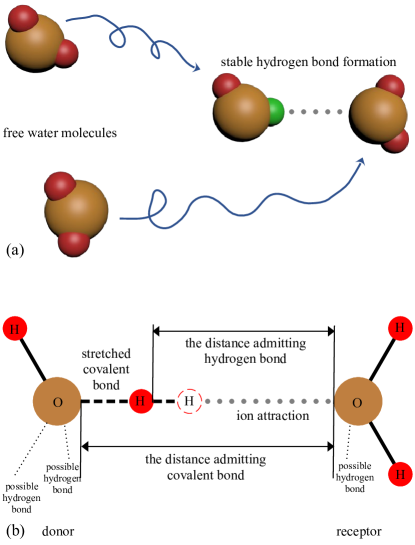
Figure 1: (online color) Hydrogen bond formation mechanism. Scale model of two $\rm{H}_{2}\rm{O}$ molecules is shown in panel (a). Mechanism of ion attraction between hydrogen and oxygen atoms is shown in the form of a Ball–and–stick model in panel (b). Brown circles (balls) represent oxygen atom, red circles (balls) represent hydrogen atom (proton) in excited state, black solid lines stand for covalent bond and gray dotted lines represent ion attraction; especially, black dashed line indicate stretched covalent bond and green ball in panel (a) represent a proton in ground state.

Interaction between two water molecules causes micro-oscillation of the hydrogen atom in one of water molecules, it allows hydrogen bonds to form between water molecules, but this process does not break covalent bond. The hydrogen bond formation mechanism is as shown in Fig. 1. In panel (a), when two $\rm{H}_{2}\rm{O}$ molecules that are moving freely are far apart, hydrogen bond cannot form between the molecules. However, when the molecules move closer together, the hydrogen atom of one molecule and the oxygen atom of another molecule attract each other and stable hydrogen bond is obtained. In panel (b), the oxygen atom (proton) of one molecule “donor” is attracted by the oxygen atom of another molecule “receptor” to produce the tunneling effect. The proton tunneling in the normal state does not destroy the covalent bond between proton and its parent molecule, but only deforms it. In the case without considering of electrons, the effect of some stretching of the covalent bond on the hydrogen bond formation is ignored, and it is considered as a normal state with a covalent bond to avoid cluttering the target model. In the model with electrons, this difference is no longer ignored. Theoretically, in addition to 2 covalent bonds, for the oxygen atom, there are actually 2 more hydrogen bonds with protons from neighboring molecules. The oxygen atom and its covalent and hydrogen bonds form a tetrahedron.

A hydrogen bond between water molecules occurs when they approach each other at a distance $|0\rangle_{dist}$, allowing one of the protons, covalently bonded to the parent molecule, to tunnel between it and another neighbouring molecule, while maintaining the existing covalent bond. The qubit $|d\rangle_{dist}$ describing the relative position of proton in the system, is introduced, and $d\in\{-1,0,1,2\}$. $dist=2$ means that the molecules are separated by a large distance, at which the formation of a hydrogen bond is impossible in principle. The state $dist=1$ means that the molecules are approaching each other at a critical distance, and although it does not allow the creation of a hydrogen bond, it allows the molecules to tunnel to the state $dist=0$, where the bond becomes possible. The state $dist=-1$ means the presence of a stable hydrogen bond, here it is an irreversible process. The influence of temperature on formation of hydrogen bond is investigated, because change of temperature will cause inflow of phonon. Thence, in this situation this process becomes reversible, that means the breaking of hydrogen bonds becomes possible.

A term of the Hamiltonian of the form $H_{i}Cond(A)$ with the condition operator $Cond(A)$ means that if the Hamiltonian $H_{i}$ has the form

$$H_{i}=H_{i}^{basis}+H_{i}^{cogerence}$$ (6)

where $H_{i}^{basis}$ is diagonal in the standard basis, and $H_{i}^{cogerence}$ is not diagonal in this basis, then the term $H_{i}^{basis}$ is added to the total Hamiltonian in any case, and $H_{i}^{cogerence}$ is added only if the condition $A$ is satisfied. This remark about the conditional Hamiltonian will be valid for further models as well. This method achieves equality of rest energies for all terms of the general Hamiltonian. So the condition operator $Cond$ means only the inclusion of coherent terms in the Hamiltonian. For example, the proton (and, subsequently, the electron) jumps only if $d=0$, that is, when the molecules are close. But in this case, the stationary energy of both the proton and the electron is always present in the Hamiltonian; only at a large distance between the molecules is it as if “frozen”, and does not lead to a change in the state of the proton (and, subsequently, the electron), and as soon as the molecules are close, the motions of these particles begin. The standard basis thus turns out to be distinguished from all others. In this work, a single hydrogen bond between a pair of water molecules, which will be extended to more hydrogen bonds using Eq. (6) in the future, is considered.

Hydrogen bonding is a fundamental interaction in chemistry and biology, playing a crucial role in the structure and function of a wide range of molecules, from water and small organic compounds to large biomolecules like DNA and proteins. Although there is no exact universal value for the time of hydrogen bond formation, it can be assumed that it can be in the range from femtoseconds to picoseconds, that is, from $10^{-15}$ to $10^{-12}$ seconds. This is due to the fact that the formation of hydrogen bonds involves the reorganization of electron clouds — a very fast quantum mechanical process. Time scale measurements of hydrogen bond dynamics can be performed using ultrafast spectroscopy techniques [50, 51, 52].

II.2 States and Hamiltonian

In Sec. II.1, the hydrogen bond model of a pair of $\rm{H}_{2}\rm{O}$ molecules is proposed, and the basic state is represented by the following form

$$|d\rangle_{dist}|p\rangle_{prot}|n\rangle_{phn}$$ (7)

where the first qubit $|d\rangle_{dist}$ is the relative position of two water molecules, which is detailed defined in Sec. II.1; the second quantum bit $|p\rangle_{prot}$ is the state corresponding to the proton, $p=0$ — proton is in the ground state $|\Phi_{0}^{pr}\rangle$ and $p=1$ — proton is in the excited state $|\Phi_{1}^{pr}\rangle$; the third qubit $|n\rangle_{phn}$ is the number of thermal phonon corresponding to the hydrogen bond. Here a special case of our model, where at most one phonon is pumped into the system (at this time, $n_{av}=1$), is proposed. When a hydrogen bond is formed, a phonon is emitted. When a hydrogen bond is broken, the phonon is absorbed.

According to Eq. (7), when $n_{av}=1$, the Hilbert space of the $\rm{H}_{2}\rm{O}$-related hydrogen bond model will consist of the following 7 basic states, which are shown in Tab. 1. And the Ball-and-stick forms of these states are shown in Fig. 2.

Qubit	Description
$|2\rangle|1\rangle|0\rangle$	Broken state
$|1\rangle|1\rangle|0\rangle$	Critical state
$|0\rangle|1\rangle|0\rangle$	Stretched and excited state
$|0\rangle|0\rangle|1\rangle$	Stretched and ground state with a phonon
$|0\rangle|0\rangle|0\rangle$	Stretched and ground state without a phonon
$|-1\rangle|0\rangle|1\rangle$	Stable state with a phonon
$|-1\rangle|0\rangle|0\rangle$	Stable state without a phonon

Table 1: Quantum states involving in evolution. The evolution involves a total of 7 states. For convenience, the following modifiers is used to define different states: “broken” means hydrogen bond is broken and two molecules are free; “critical” means the critical point of hydrogen bond formation and breaking is obtained; “stretched” means the proton of donor moves toward receptor due to the ion attraction and covalent bond is stretched; “excited” means proton state is excited; “ground” means proton state is ground; “stable” means hydrogen bond is stable. Especially, when the state is stable, it must also be stretched and ground. Besides states $|-1\rangle|0\rangle|1\rangle$ and $|-1\rangle|0\rangle|0\rangle$, the rest states can all defined as “unstable”. In addition, there are two cases for the ground state: with/without a phonon.

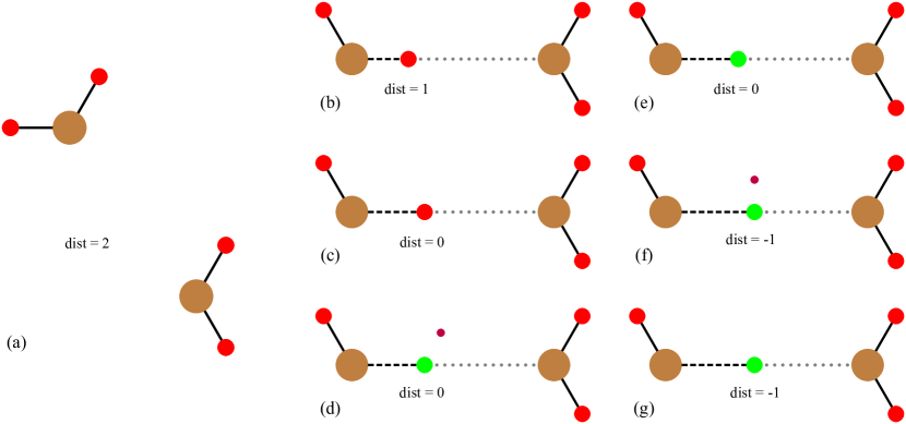
Figure 2: (online color) Quantum states involved in evolution. (a) $\sim$ (g) correspond to seven states for $\rm{H}_{2}\rm{O}$-related hydrogen bond model: $|2\rangle|1\rangle|0\rangle,\ |1\rangle|1\rangle|0\rangle,\ |0\rangle|1\rangle|0\rangle,\ |0\rangle|0\rangle|1\rangle,\ |0\rangle|0\rangle|0\rangle,\ |-1\rangle|0\rangle|1\rangle,\ |-1\rangle|0\rangle|0\rangle$. Here brown, red, green and purple circles represent oxygen atom, proton with excited state, proton with ground state and thermal phonon, respectively; solid and dashed black lines stand for ordinary and stretched covalent bond, respectively; ion attraction is denoted by gray dotted lines.

$H_{hyd}$ is represented by the Hamiltonian of a system of two water molecules connected by hydrogen bond and has the following form

$$H_{hyd}=H_{dist}Cond(p=1)+H_{prot}Cond(d=0)$$ (8)

where $H_{dist}$ describes proton tunneling energy and $H_{prot}$ describes Hamiltonian for transitions. $Cond(p=1)$ and $Cond(d=0)$ are conditional operators. The rotating wave approximation (RWA) is particularly useful in systems where the interactions are resonant or nearly resonant [53]. RWA is taken into account and the Hamiltonians is described in following form

• $H_{dist}$ is defined as follows

  $$H_{dist}=\hbar\omega_{dist}\sigma^{{\dagger}}_{dist}\sigma_{dist}+g_{dist}\left(\sigma^{{\dagger}}_{dist}+\sigma_{dist}\right)$$ (9)

  where $\omega_{dist}$ is frequency for tunneling of phonons; $g_{dist}$, which is located on the non-diagonal line of the Hamiltonian, is the strength for tunneling of proton. And definitions of operators $\sigma_{dist}$ and $\sigma^{{\dagger}}_{dist}$ are as follows

  $$\sigma_{dist}|1\rangle_{dist} =|0\rangle_{dist}$$ (10)

  $$\sigma_{dist}^{{\dagger}}|0\rangle_{dist} =|1\rangle_{dist}$$

• $H_{prot}$ is defined as follows

  $$H_{prot} =\hbar\omega_{phn}a^{{\dagger}}_{phn}a_{phn}+\hbar\omega_{prot}\sigma^{{\dagger}}_{prot}\sigma_{prot}$$ (11)

  $$+g_{prot}\left(a_{phn}\sigma^{{\dagger}}_{prot}+a^{{\dagger}}_{phn}\sigma_{prot}\right)$$

  where $\omega_{phn}$ is phononic mode, $\omega_{prot}$ is mode for transitions of proton, and $\omega_{phn}=\omega_{prot}$; $g_{prot}$ is the strength for transitions of proton. And definitions of operators $a^{{\dagger}}_{phn}\sigma_{prot}$ and $a_{phn}\sigma_{prot}^{{\dagger}}$ are as follows

  $$a^{{\dagger}}_{phn}\sigma_{prot}|1\rangle_{prot}|0\rangle_{phn} =|0\rangle_{prot}|1\rangle_{phn}$$ (12)

  $$a_{phn}\sigma_{prot}^{{\dagger}}|0\rangle_{prot}|1\rangle_{phn} =|1\rangle_{prot}|0\rangle_{phn}$$

The complete quantum system ultimately constructed by the total Hamiltonian $H_{hyd}$ can be intuitively represented in the form of a network, which is shown in Fig. 3. Interactions, dissipations and inflows between states can be intuitively seen in this figure, and the energy wandering of the whole system is determined clearly.

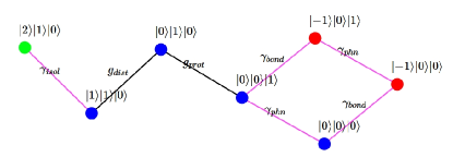
Figure 3: (online color) Network of quantum states and energy wandering. The quantum system consists of several states, between which there are some potential interactions, dissipations and inflows. In this figure, the dots represent the states and the edges — interactions, dissipations and inflows. Red dots stand for the states corresponding to the formation of stable hydrogen bond; green dot represents the state corresponding to the case that hydrogen bond is broken and two molecules are free; blue dots represent the states corresponding to unstable hydrogen bond. Black edges stand for the interactions ($g_{dist}$ and $g_{prot}$); purple edges represent the dissipations and inflows. In particular, $\gamma_{isol}$ includes both dissipation $\gamma_{isol}^{out}$ from state $|1\rangle|1\rangle|0\rangle$ to state $|2\rangle|1\rangle|0\rangle$ and inflow $\gamma_{isol}^{in}$ from state $|2\rangle|1\rangle|0\rangle$ to state $|1\rangle|1\rangle|0\rangle$.

II.3 Quantum master equation

The influence of temperature on the formation of a hydrogen bond requires the use of a QME and the introduction of one decoherence factor related to the qubit $|n\rangle_{phn}$ of the basic state

$$A_{phn}|1\rangle_{phn}=|0\rangle_{phn}$$ (13)

$$A_{phn}^{{\dagger}}|0\rangle_{phn}=|1\rangle_{phn}$$

where $\gamma_{phn}$ is the dissipation intensity for the escape of phonons from cavity to external environment. Similarly, the introduction of two quasi-decoherence factors, which are similar to the form of $A_{phn},\ A_{phn}^{{\dagger}}$ and related to the qubit $|d\rangle_{dist}$ of the basic state, is as follows

$$A_{bond}|0\rangle_{dist}=|-1\rangle_{dist}$$ (14)

$$A_{bond}^{{\dagger}}|-1\rangle_{dist}=|0\rangle_{dist}$$

$$A_{isol}|1\rangle_{dist} =|2\rangle_{dist}$$ (15)

$$A_{isol}^{{\dagger}}|2\rangle_{dist} =|1\rangle_{dist}$$

where $\gamma_{bond}$ is the dissipation intensity for the micromotions of molecules that must calm down to form a bond, and $\gamma_{isol}$ is the dissipation intensity for the macromotions of molecules in the medium. And

The QME, which is also called Lindbladian, is used to describe the time-dependent evolution of the density matrix of an open quantum system, which allow us to obtain the dependence of the probability of hydrogen bond formation on temperature. It can be seen as a natural result of the coupling between the system and the environment under the lowest-order perturbation and Markov approximation

$$i\hbar\dot{\rho}=[H,\rho]+i\mathcal{L}(\rho)$$ (16)

where $\mathcal{L}=L^{in}+L^{out}$. $L^{in}$ describes the inflow process and $L^{out}$ describes the dissipation process. And

$$L^{in}(\rho)=\gamma^{in}\left(A^{\dagger}\rho A-\frac{1}{2}\left(AA^{\dagger}\rho+\rho AA^{\dagger}\right)\right)$$ (17)

$$L^{out}(\rho)=\gamma^{out}\left(A\rho A^{\dagger}-\frac{1}{2}\left(A^{\dagger}A\rho+\rho A^{\dagger}A\right)\right)$$ (18)

where $A$ and $A^{\dagger}$ can be replaced by $A_{bond},\ A_{isol},\ A_{phn},\ A_{bond}^{\dagger},\ A_{isol}^{\dagger}$ and $A_{phn}^{\dagger}$. The full form of the operator $\mathcal{L}$ with consideration of all types of inflows and dissipations is shown in Appx. A.

III Numerical method

To solve the QME, various numerical methods such as the Euler method. The iteration consists of three steps. The first step is to calculate the unitary evolution of the density matrix

$$\widetilde{\rho}(t+\Delta t)=e^{\frac{-iH\Delta t}{\hbar}}\rho(t)e^{\frac{iH\Delta t}{\hbar}}.$$ (19)

where $\Delta t$ is the iteration time step and the second step is to apply the Lindblad superoperator (17) and (18) to the density matrix $\rho(t+\Delta t)$ at this moment

$$\rho(t+\Delta t)=\widetilde{\rho}(t+\Delta t)+\frac{1}{\hbar}\mathcal{L}(\widetilde{\rho}(t+\Delta t))\Delta t.$$ (20)

The third step is to scale the density matrix to maintain its positive definite, Hermitian matrix, unit trace and other properties.

In addition to the Euler method, there is also the more accurate Runge-Kutta method. For quantum systems with particularly large states, the Monte Carlo wave function method [54] or the pure state vector method [55] can achieve higher computational efficiency. The $\rm{H}_{2}\rm{O}$-related hydrogen bond model contains a total of 7 states, so using the Euler method makes it easier for us to study the effects of various interactions and dissipations on evolution.

When solving the QME using the Euler method, The order of magnitude of the time step $\Delta t$ usually depends on the unit of the system’s Hamiltonian and the units of other related parameters. In optical Cavity QED experiments with high finesse optical resonators [56] or microwave resonators [57], the time step is determined by the measurement time, which is around 1 $\mu s$. However, for a single hydrogen bond, the time step reference measurement time of 1 $\mu s$ is not appropriate. Therefore, the characteristic time scale $\tau$ of the simulated dissipative quantum system is adopted, which can be estimated from the system energy and the reduced Planck constant

$$\tau=\frac{\hbar}{E}$$ (21)

where $E$ is the energy of the quantum system and the intensity factor $\gamma$ is usually smaller than $E$. When implementing the Euler method numerically, the time step $\Delta t$ should be significantly smaller than the characteristic time scale.

The energy of a single hydrogen bond $E_{H-bond}$ can be estimated from the average energy of hydrogen bonds in water and Avogadro’s constant, which is approximately $0.217655\ eV$. Using joule as the energy unit may cause machine error due to too small parameters, so $eV$ is used as the energy unit. And the characteristic time scale $\tau$ is about $3.175316\times 10^{-15}\ s$. The detailed calculation process is shown in Appx. B.

IV Simulations and results

For convenience, the Hilbert space is divided into two subspaces: stable hydrogen bond subspace and unstable hydrogen bond subspace. Stable subspace includes states $|-1\rangle|0\rangle|1\rangle$ and $|-1\rangle|0\rangle|0\rangle$, and unstable subspace includes the rest. The stable subspace can be defined as follows

$$|\rm{O}\cdots\rm{H}\rangle=c^{\prime}|-1\rangle|0\rangle|1\rangle+c^{\prime\prime}|-1\rangle|0\rangle|0\rangle$$ (22)

where $c^{\prime},\ c^{\prime\prime}$ are the normalization factors.

The physical determination of the time of hydrogen bond formation involves a combination of experimental techniques such as ultrafast infrared spectroscopy [51], which determines the time between $0.5ps$ and $1ps$ ($10^{-12}s$). Therefore, in all simulations, two reference parameters are proposed: $g=2\times 10^{-3}\rm{eV},\ \gamma=5\times 10^{-3}\rm{eV}$. All interaction strengths $g_{dist}$ and $g_{prot}$ below are expressed in terms of reference parameter $g$ and all dissipation intensities $\gamma_{isol}^{out}$, $\gamma_{bond}^{out}$ and $\gamma_{phn}^{out}$ below are expressed in terms of reference parameter $\gamma$. Especially, inflow intensities $\gamma_{isol}^{in}$, $\gamma_{bond}^{in}$ and $\gamma_{phn}^{in}$ are not used directly in simulations, but ratios $\mu_{isol}$, $\mu_{bond}$ and $\mu_{phn}$ (inflow intensity divided by dissipation intensity), defined in Eq. (5), are used instead. Except for the above mentioned parameters which will change during the simulation, the remaining parameters are all fixed. Especially, $\hbar\omega_{prot}+\hbar\omega_{dist}=E_{H-bond}$, $\Delta t=0.01\tau$.

Various dynamic aspects of $\rm{H}_{2}\rm{O}$-related hydrogen bond model are shown as below five subsections.

IV.1 Comparison between unitary and dissipative evolutions

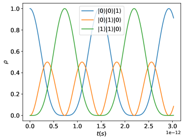
Figure 4: (online color) The unitary evolution. The initial state is $|0\rangle|0\rangle|1\rangle$. $g_{prot}=g_{dist}=g$ and $\gamma_{isol}^{out}=\gamma_{bond}^{out}=\gamma_{phn}^{out}=0$.

Firstly, in closed system without the dissipation intensities, the unitary evolution with only three basic states ($|0\rangle|0\rangle|1\rangle$, $|0\rangle|1\rangle|0\rangle$ and $|1\rangle|1\rangle|0\rangle$) is obtained. The unitary evolution considering only the interaction between particles and fields is calculated by the Schrödinger equation.

$$i\hbar\dot{\rho}=[H,\rho]=H\rho-\rho H$$ (23)

For the unitary evolution, the calculation method only needs to adopt the Eq. (19). The initial state is $|0\rangle|0\rangle|1\rangle$ — stretched and ground state with a phonon. The unitary evolution, considering $g_{prot}=g_{dist}=g$, is shown in Fig. 4. The three obtained curves, representing the states $|0\rangle|0\rangle|1\rangle$, $|0\rangle|1\rangle|0\rangle$ and $|1\rangle|1\rangle|0\rangle$, oscillate periodically.

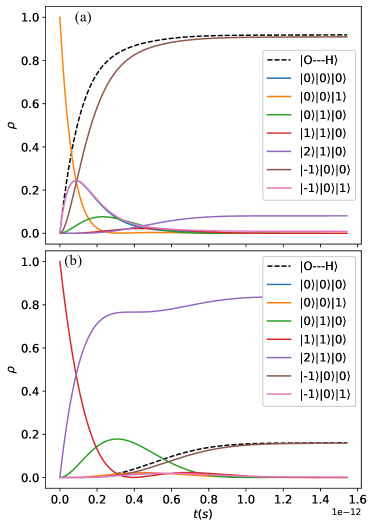
Figure 5: (online color) The dissipative evolution. $g_{prot}=g_{dist}=g$ and $\gamma_{isol}^{out}=\gamma_{bond}^{out}=\gamma_{phn}^{out}=\gamma$. In panel (a), the initial state is $|0\rangle|0\rangle|1\rangle$; in panel (b), the initial state is $|1\rangle|1\rangle|0\rangle$. The black dashed curve corresponds to the stable hydrogen bond: the probability of $|\rm{O}\cdots\rm{H}\rangle$ is the sum of probabilities of $|-1\rangle|0\rangle|1\rangle$ and $|-1\rangle|0\rangle|0\rangle$.

Dissipation intensities are taken into consideration to calculate the dissipative evolution of an open system with thermal phonon entering and exiting. The QME is numerically calculated using Eq. (20). In addition to initial state $|0\rangle|0\rangle|1\rangle$, the initial state $|1\rangle|1\rangle|0\rangle$ — critical state, is also considered. Critical state means the critical point of hydrogen bond breaking is reached. Comparison between these two initial states is carried out in Fig. 5. As shown in both panels, the periodic oscillations disappear, replaced by dissipations. The time of hydrogen bond formation is about $1\rm{ps}$ ($10^{-12}s$) before the probability reaches a stable level. In panel (a), the system tends to form a stable hydrogen bond when the initial state is $|0\rangle|0\rangle|1\rangle$. On the contrary, in panel (b), the system tends to break the hydrogen bond when the initial state is $|1\rangle|1\rangle|0\rangle$. This is because the state $|0\rangle|0\rangle|1\rangle$ is stretched and ground, and the proton of donor at this time is at lower energy lever. Thus, it is more inclined to form a stable hydrogen bond. The state $|1\rangle|1\rangle|0\rangle$ means that the critical point of hydrogen bond formation and breaking is obtained, and the hydrogen bond breaks more easily to release two free water molecules.

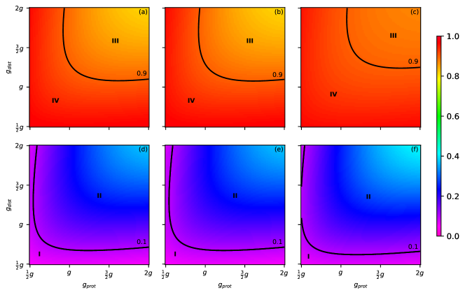
Figure 6: (online color) Effect of different interactions strengths $g_{dist}$ and $g_{prot}$ on the hydrogen bond formation. The first row of panels is the dissipative evolution result of the initial state $|0\rangle|0\rangle|1\rangle$. The second row of panels is the dissipative evolution result of the initial state $|1\rangle|1\rangle|0\rangle$. The values of $g_{dist}$, $g_{prot}$ range from $0.5g$ to $2g$ and the intensities of all dissipations are fixed: $\gamma_{isol}^{out}=\gamma_{bond}^{out}=\gamma_{phn}^{out}=\gamma$. The first column corresponds to the case that $\mu_{isol}=\mu_{bond}=\mu_{phn}=0$; the second column corresponds to the case that $\mu_{isol}=\mu_{bond}=0,\ \mu_{phn}=0.01$; the third column corresponds to the case that $\mu_{isol}=\mu_{bond}=\mu_{phn}=0.01$. The color of the heat map represents the probability of stable hydrogen bond formation (the probability of $|\rm{O}\cdots\rm{H}\rangle$ when system reaches a stable point after a long time). Regions I, II, III, and IV are the regions of probability within $[0,\ 0.1),\ [0.1,\ 0.5),\ [0.5,\ 0.9)$ and $[0.9,\ 1]$, respectively. These definitions of regions I$\sim$IV are also apply to Figs. 7 and 8.

IV.2 The effect of interactions on evolution

Result of Fig. 6 is shown as heat maps, where the color dots represent the probability of stable hydrogen bond formation at $t\to\infty$. Here $\infty$ is obtained, when the system tends to stabilize and probabilities of states approach constant values. In the next subsections, results of Figs. 7, 8 and 11 are also represented as heat maps at $t\to\infty$.

The effect of interaction strengths $g_{dist}$ and $g_{prot}$ on the evolution and the hydrogen bond formation is obtained in Fig. 6, where the values of $g_{dist}$, $g_{prot}$ range from $0.5g$ to $2g$. All dissipation intensities are fixed: $\gamma_{isol}^{out}=\gamma_{bond}^{out}=\gamma_{phn}^{out}=\gamma$. Under different initial states, the dissipative evolution will eventually reach probabilistic stability after long-term evolution.

In the first row of Fig. 6, when the initial state is $|0\rangle|0\rangle|1\rangle$, result is found that the larger interaction strengths $g_{dist}$ and $g_{prot}$, the lower the probability of forming stable hydrogen bond. However, in the second row, when initial state is $|1\rangle|1\rangle|0\rangle$, the opposite result is found. In summary, in the case of $|0\rangle|0\rangle|1\rangle$, the interaction strengths have the negative effect on the formation of stable hydrogen bond — hindering the hydrogen bond formation; in the case of $|1\rangle|1\rangle|0\rangle$, the interaction strengths have the positive effect on the formation of stable hydrogen bond — promoting the hydrogen bond formation. Besides, when the initial state is $|0\rangle|0\rangle|1\rangle$, the probabilities on the heat maps are all on the range of $[0.5,\ 1]$; When the initial state is $|1\rangle|1\rangle|0\rangle$, the probabilities on the heat maps are all on the range of $[0,\ 0.5)$.

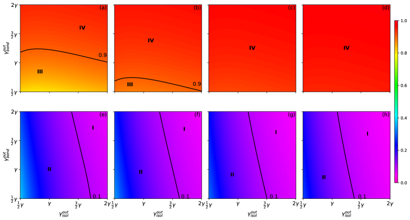
Figure 7: (online colar) Effect of different dissipations intensities $\gamma_{isol}^{out}$, $\gamma_{bond}^{out}$ and $\gamma_{phn}^{out}$ on the hydrogen bond formation. $g_{prot}=g_{dist}=g$. The first row of panels is the result of the initial state $|0\rangle|0\rangle|1\rangle$. The second row of panels is the result of the initial state $|1\rangle|1\rangle|0\rangle$. The values of $\gamma_{isol}^{out}$, $\gamma_{bond}^{out}$ range from $0.5\gamma$ to $2\gamma$ and the values of $\gamma_{phn}^{out}$ from the first column to the fourth column correspond to $\frac{1}{2}\gamma,\ \gamma,\ \frac{3}{2}\gamma$ and $2\gamma$, respectively. The definitions of regions II, III and IV are all defined in Fig. 6.

In this section, the effects of the inflows intensities $\gamma_{phn}^{in}$, $\gamma_{bond}^{in}$ and $\gamma_{isol}^{in}$ are investigated. The first column corresponds to the case that inflows are prohibited: $\mu_{isol}=\mu_{bond}=\mu_{phn}=0$, that is to say, $\gamma_{isol}^{in}=\gamma_{bond}^{in}=\gamma_{phn}^{in}=0$. The second column corresponds to the case that only phonon inflow is permitted: $\mu_{isol}=\mu_{bond}=0,\ \mu_{phn}=0.01$. The third column corresponds to the case that all inflows are permitted: $\mu_{isol}=\mu_{bond}=\mu_{phn}=0.01$. Comparing the second and the third columns with the first column, result is found that the addition of weak inflows actually promotes the formation of hydrogen bond, regardless of whether the initial state is $|0\rangle|0\rangle|1\rangle$ or $|1\rangle|1\rangle|0\rangle$. For easy observation, we use the dividing lines. In the first row from panel (a) to panel (c), it is easy to find that the solid dividing line representing the probability of $0.9$ is shifted to the upper right. At the same time, the area of region III of probability with $[0.5,\ 0.9)$ decreases and the area of region IV of probability with $[0.9,\ 1]$ increases. This means the weak inflows promotes the hydrogen bond formation when initial state is $|0\rangle|0\rangle|1\rangle$. Similarly, in the second row from panel (d) to panel (f), the solid dividing line representing the probability of $0.1$ is shifted to the lower left. At the same time, the area of region I of probability with $[0,\ 0.1)$ decreases and the area of region II of probability with $[0.1,\ 0.5]$ increases. This means the weak inflows also promotes the hydrogen bond formation when initial state is $|1\rangle|1\rangle|0\rangle$.

In addition to the above results, the effect of different interactions strengths on the time required for the system to reach stable is also obtained: the smaller interactions strengths, the more time required to reach stable. When $g_{dist}=g_{prot}=0.5g$ system requires the most time to reach stable.

IV.3 The effects of dissipations on evolution

The effects of dissipations on evolution are studied. The parameters being studied are $\gamma_{bond}^{out},\ \gamma_{phn}^{phn},\ \gamma_{isol}^{out}$. All interactions strengths are fixed: $g_{dist}=g_{dist}=g$. The values of $\gamma_{isol}^{out}$ and $\gamma_{bond}^{out}$ range from $0.5\gamma$ to $2\gamma$. The values of $\gamma_{phn}^{out}$ from the first column to the fourth column correspond to $0.5\gamma,\ \gamma,\ 1.5\gamma$ and $2\gamma$, respectively. Under different initial states, the dissipative evolution will also eventually reach probabilistic stability after long-term evolution.

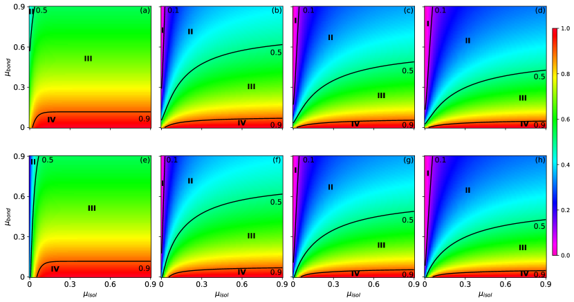
Figure 8: (online colar) Effect of different inflows intensities $\mu_{isol}$, $\mu_{bond}$ and $\mu_{phn}$ on the hydrogen bond formation. $g_{prot}=g_{dist}=g$, $\gamma_{isol}^{out}=\gamma_{bond}^{out}=\gamma_{phn}^{out}=\gamma$. The first row of panels is the result of the initial state $|0\rangle|0\rangle|1\rangle$. The second row of panels is the result of the initial state $|1\rangle|1\rangle|0\rangle$. The values of $\mu_{isol}$, $\mu_{bond}$ range from $0$ to $0.9$ and the values of $\mu_{phn}$ from the first column to the fourth column correspond to $0,\ 0.3,\ 0.6$ and $0.9$, respectively. The definitions of regions I, II, III and IV are all shown in Fig. 6.

In the first row of Fig. 7, when the initial state is $|0\rangle|0\rangle|1\rangle$, result is found that the larger dissipations intensities $\gamma_{isol}^{out}$ and $\gamma_{bond}^{out}$, the larger the probability of forming stable hydrogen bond. However, in the second row, when initial state is $|1\rangle|1\rangle|0\rangle$, the opposite result is found. In the first row from panel (a) to panel (d), it is easy to find that the solid dividing line representing the probability of $0.9$ is shifted from top to bottom until it disappears. At the same time, the area of region III of probability with $[0.5,\ 0.9)$ decreases to $0$ and the area of region IV of probability with $[0.9,\ 1]$ increases to $1$. This means the intensity $\gamma_{phn}^{out}$ promotes the hydrogen bond formation when initial state is $|0\rangle|0\rangle|1\rangle$. Similarly, in the second row from panel (e) to panel (h), the solid dividing line representing the probability of $0.1$ is shifted from right to left. At the same time, the area of region I of probability with $[0,\ 0.1)$ increases and the area of region II of probability with $[0.1,\ 0.5]$ decreases. This means intensity $\gamma_{phn}^{out}$ hinders the hydrogen bond formation when initial state is $|1\rangle|1\rangle|0\rangle$. In summary, in the case of $|0\rangle|0\rangle|1\rangle$, the all dissipations intensities have the positive effect on the formation of stable hydrogen bond; in the case of $|1\rangle|1\rangle|0\rangle$, the dissipations intensities have the negative effect on the formation of stable hydrogen bond. Similar to the Fig. 6, when the initial state is $|0\rangle|0\rangle|1\rangle$, the probabilities on the heat maps are all on the range of $[0.5,\ 1]$; When the initial state is $|1\rangle|1\rangle|0\rangle$, the probabilities on the heat maps are all on the range of $[0,\ 0.5)$.

IV.4 The effects of inflows on evolution

Temperature is also an important factor, it will cause inflows of phonons. According to Eq. (5), $\mu_{bond},\ \mu_{isol}$ and $\mu_{phn}$ are described as follows

$$\mu_{isol} =\frac{\gamma_{isol}^{in}}{\gamma_{isol}^{out}}=e^{\frac{-\hbar\omega_{isol}}{KT_{isol}}}$$ (24a)

$$\mu_{bond} =\frac{\gamma_{bond}^{in}}{\gamma_{bond}^{out}}=e^{\frac{-\hbar\omega_{bond}}{KT_{bond}}}$$ (24b)

$$\mu_{phn} =\frac{\gamma_{phn}^{in}}{\gamma_{phn}^{out}}=e^{\frac{-\hbar\omega_{phn}}{KT_{phn}}}$$ (24c)

where $\omega_{isol}=\omega_{bond}=\omega_{phn}$, $\mu_{isol}<1,\ \mu_{bond}<1,\ \mu_{phn}<1$. When $\gamma_{isol}^{out}=\gamma_{bond}^{out}=\gamma_{phn}^{out}=\gamma$, $\mu_{bond},\ \mu_{isol}$ and $\mu_{phn}$ are positively correlated with inflows intensities $\gamma_{isol}^{in}$, $\gamma_{bond}^{in}$ and $\gamma_{phn}^{in}$, respectively; they are also positively correlated with temperature $T_{isol}$, $T_{bond}$ and $T_{phn}$, respectively. For the convenience of research, $\mu_{isol}$, $\mu_{bond}$ and $\mu_{phn}$ can be used to study the effects of inflows or temperatures on evolution.

According to the result in Fig. 8, no matter the initial state is $|0\rangle|0\rangle|1\rangle$ or $|1\rangle|1\rangle|0\rangle$, the larger $\mu_{isol}$ and the smaller $\mu_{bond}$, the larger the probability of forming stable hydrogen bond. This means $\mu_{isol}$ promotes the hydrogen bond formation, but $\mu_{bond}$ hinders the hydrogen bond formation. In the first row from panel (a) to panel (d), it is easy to find that all three solid dividing lines representing the probability of $0.1$, $0.5$ and $0.9$ respectively are shifted from left to right. At the same time, the area of region I of probability with $[0,\ 0.1)$ and the area of region II of probability with $[0.1,\ 0.5)$ both increases, the area of region III of probability with $[0.5,\ 0.9]$ and the area of region IV of probability with $[0.9,\ 1]$ both decreases. This means the $\mu_{phn}$ hinders the hydrogen bond formation no matter the initial state is $|0\rangle|0\rangle|1\rangle$ or $|1\rangle|1\rangle|0\rangle$. In summary, the $\mu_{isol}$ has the positive effect on the formation of stable hydrogen bond; however, the $\mu_{bond}$ and $\mu_{phn}$ have the negative effect on it. Different to the Figs. 6 and 7, the probabilities on the heat maps are all on the range of $[0,\ 1]$.

IV.5 The effects of external impulses on evolution

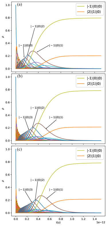
Figure 9: (online color) Effect of external impulses of phonons on the hydrogen bond formation. $g_{dist}=g_{prot}=g$, $\gamma_{isol}^{out}=\gamma_{bond}^{out}=\gamma_{ph}^{out}=\gamma$, $\mu_{isol}=\mu_{bond}=0$, $\mu_{phn}=0.01$. The number of phonons varies in different panels: 10 in panel (a), 20 in (b), 30 in (c).

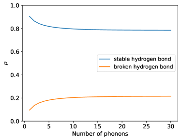
Figure 10: (online color) Effect of number of phonons on the hydrogen bond formation. $g_{dist}=g_{prot}=g$, $\gamma_{isol}^{out}=\gamma_{bond}^{out}=\gamma_{ph}^{out}=\gamma$, $\mu_{isol}=\mu_{bond}=0$, $\mu_{phn}=0.01$. The number of phonons is within $[1,\ 30]$.

As mentioned before, the micro-oscillation of protons will affect the stability of hydrogen bonds. Therefore, in this section, the phonon energy to enhance the effect of this micro-oscillation is strengthened and the changes in the probability of stable hydrogen bond formation is observed. In order to incorporate the effect of external impulses on proton tunneling into the model, the initial number of phonons is changed (in order to reduce interference factors, the inflows intensities $\gamma_{isol}^{in}$ and $\gamma_{bond}^{in}$ is not considered at this time).

By analyzing Fig. 9, result is found that when the number of phonons is large, changing the number of phonons in the initial state (external momentum) has little effect on the probability of hydrogen bond stability. Even when the number of phonons increases to 30, the probability of a stable hydrogen bond in this model remains stable at around 0.8. When the number of a specific type of phonon is large enough, the expected bond length of the hydrogen bond will tend to a stable value, and the stability of hydrogen bonds decreases slightly. This rule not only appears in the O-H$\cdots$O system, but also in the N-H$\cdots$O system [58]. Therefore, the number of phonons in a smaller range is next controlled.

In Fig. 10, the stability of hydrogen bonds increases with the increase of the number of phonons. When the number of phonons increases, the probability of a stable hydrogen bond increases, while the probability of a broken hydrogen bond decreases, and both tend to a stable value.

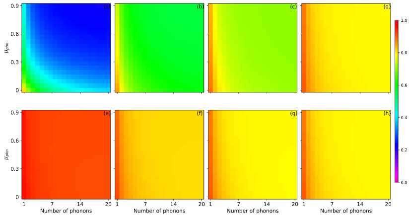
Figure 11: (online color) Effect of the initial phonon number and phonon inflow on the hydrogen bond formation. $g_{dist}=g_{prot}=g$. The initial state is $|0\rangle|0\rangle|N_{phn}\rangle$. In the first row, $\gamma_{isol}^{out}=\gamma_{phn}^{out}$ is fixed, while $\gamma_{bond}^{out}$ is varied in the four panels: $\gamma_{bond}^{out}$ = 0.1 in panel (a), $\gamma_{bond}^{out}$ = 0.4 in panel (b), $\gamma_{bond}^{out}$ = 0.7 in panel (c), $\gamma_{bond}^{out}$ = 1 in panel (d). In the second row, $\gamma_{bond}^{out}=\gamma_{phn}^{out}$ is fixed, while $\gamma_{isol}^{out}$ is varied in the four panels: $\gamma_{isol}^{out}$ = 0.1 in panel (e), $\gamma_{isol}^{out}$ = 0.4 in panel (f), $\gamma_{isol}^{out}$ = 0.7 in panel (g), $\gamma_{isol}^{out}$ = 1 in panel (h).

In Fig.11 the effect of external impulse and phononic temperature on the probability of stable hydrogen bond formation is obtained. From the horizontal axis, as the external impulse (the number of phonons in the initial state) increases, the hydrogen bond stability decreases. From the vertical axis, the same conclusion applies to the phononic temperature $\mu_{ph}$. Their increase will make the micro-oscillations of proton more intense, thereby reducing the stability of hydrogen bonds.

From the four panels (a),(b),(c),(d) in the first row, as $\gamma_{bond}^{out}$ increases, the temperature of the heat map increases, indicating that it is positively correlated with the stability of hydrogen bonds. In addition, by comparing the columns of these four pictures, the increase in $\gamma_{bond}^{out}$ also reduces the effect of $\mu_{phn}$ on the probability of stable hydrogen bond formation, making the temperature of the heat map gradually approach inversely proportional to the number of phonons. From the four panels in the second row, as $\gamma_{isol}^{out}$ increases, the temperature of the heat map decreases, indicating that it is negatively correlated with the stability of hydrogen bonds. By comparing panel (e) with panels (f), (g), and (h), when $\gamma_{isol}^{out}$ is small enough, the temperature of the heat map hardly changes with the increase in the number of phonons, indicating that the probability of stable hydrogen bonds is high.

V Concluding discussion and future work

In this paper, the various dynamic aspects of $\rm{H}_{2}\rm{O}$-related hydrogen bond model are investigated. And the results show the nontrivial dependence of the hydrogen bond formation on the parameters. Some analytical results of it are derived as follows

• In Sec. IV.1, the periodical oscillations of closed system are obtained. Once the dissipations of the non-ideal system is introduced, the oscillations disappear and two final results are obtained: the formation of stable hydrogen bond or the complete breaking of hydrogen bond. Different initial states lead to different results: the system tends to form a stable hydrogen bond when the initial state is $|0\rangle|0\rangle|1\rangle$; the system tends to break the hydrogen bond when the initial state is $|1\rangle|1\rangle|0\rangle$.

• In Sec. IV.2, the effect of interactions on evolution is studied. When the initial state is $|0\rangle|0\rangle|1\rangle$, the larger the interaction strengths, the harder to form a hydrogen bond. On the contrary, when the initial state is $|1\rangle|1\rangle|0\rangle$, the larger the interaction strengths, the easier to form a hydrogen bond.

• In Sec. IV.3, the effect of dissipations on the hydrogen bond formation is studied. When the initial state is $|0\rangle|0\rangle|1\rangle$, the probability of stable hydrogen bond formation is negatively correlated with $\gamma_{isol}^{out}$ and positively correlated with $\gamma_{bond}^{out}$; when the initial state is $|1\rangle|1\rangle|0\rangle$, the probability of stable hydrogen bond formation is negatively correlated with both $\gamma_{isol}^{out}$ and $\gamma_{bond}^{out}$.

• In Sec. IV.4, the effect of inflows on the hydrogen bond formation is studied. Regardless of whether the initial state is $|0\rangle|0\rangle|1\rangle$ or $|1\rangle|1\rangle|0\rangle$, the probability of stable hydrogen bond formation is positively correlated with $\mu_{isol}$ and negatively correlated with $\mu_{bond}$.

• In Sec. IV.5, the effect of external impulses on the hydrogen bond formation is obtained. The more free phonons flow in from the outside, the lower the probability of stable hydrogen bonds forming, and as the number of phonons increases, the probability approaches a critical value.

The results show that the evolution and hydrogen bond formation can be controlled by selectively choosing system parameters. Although we only studied the dynamic aspects of simple hydrogen bond model, the results we found will be used as a basis to extend the research to more complex chemical and biological model in the future.

Appendix A Quantum master equation for the target model

The QME has the following form

$$i\hbar\dot{\rho}=[H,\rho]+i\mathcal{L}(\rho)$$ (25)

where $\mathcal{L}=L^{in}+L^{out}$. And

$$L^{in}(\rho)=\gamma_{bond}^{in}\left(A_{bond}^{\dagger}\rho A_{bond}-\frac{1}{2}\left(A_{bond}A_{bond}^{\dagger}\rho+\rho A_{bond}A_{bond}^{\dagger}\right)\right)$$ (26)

$$+\gamma_{isol}^{in}\left(A_{isol}^{\dagger}\rho A_{isol}-\frac{1}{2}\left(A_{isol}A_{isol}^{\dagger}\rho+\rho A_{isol}A_{isol}^{\dagger}\right)\right)+\gamma_{phn}^{in}\left(A_{phn}^{\dagger}\rho A_{phn}-\frac{1}{2}\left(A_{phnl}A_{phn}^{\dagger}\rho+\rho A_{phn}A_{phn}^{\dagger}\right)\right)$$

$$L^{out}(\rho)=\gamma_{bond}^{out}\left(A_{bond}\rho A_{bond}^{\dagger}-\frac{1}{2}\left(A_{bond}^{\dagger}A_{bond}\rho+\rho A_{bond}^{\dagger}A_{bond}\right)\right)$$ (27)

$$+\gamma_{isol}^{out}\left(A_{isol}\rho A_{isol}^{\dagger}-\frac{1}{2}\left(A_{isol}^{\dagger}A_{isol}\rho+\rho A_{isol}^{\dagger}A_{isol}\right)\right)+\gamma_{phn}^{out}\left(A_{phn}\rho A_{phn}^{\dagger}-\frac{1}{2}\left(A_{phn}^{\dagger}A_{phn}\rho+\rho A_{phn}^{\dagger}A_{phn}\right)\right)$$

where $\gamma_{bond}^{in}=\mu_{bond}\gamma_{bond}^{out},\ \gamma_{isol}^{in}=\mu_{isol}\gamma_{isol}^{out},\ \gamma_{phn}^{in}=\mu_{phn}\gamma_{phn}^{out}$. Here $\mu_{bond}<1,\ \mu_{isol}<1,\ \mu_{phn}<1$, thus $\gamma_{bond}^{in}<\gamma_{bond}^{out},\ \gamma_{isol}^{in}<\gamma_{isol}^{out},\ \gamma_{phn}^{in}<\gamma_{phn}^{out}$.

Appendix B Estimation of physical quantities

The average energy of hydrogen bonds in water is $21\ kJ/mol$. To convert this energy to the energy of a single hydrogen bond, estimate it by using Avogadro’s constant ($N_{A}$), the number of particles per mole of substance, which is approximately ($6.022\times 10^{23}$). Through calculation, it can be estimated that the energy of a single hydrogen bond

$$E_{H-bond} =\frac{E_{bond}}{N_{A}}$$ (28)

$$=\frac{21\times 10^{3}\ \text{[J/mol}]}{6.022\times 10^{23}\text{[molecules/mol]}}$$

$$\approx 3.32\times 10^{-20}\ [J]=0.217655\ \text{[eV]}$$

Substituting into Eq. (21) and calculating, the characteristic time scale is got as follows

$$\tau=\frac{\hbar}{E}=\frac{\hbar\times N_{A}}{E_{H-bond}}=\frac{1.0545718\times 10^{-34}\ [J\cdot s]\times 6.022\times 10^{23}\text{[molecules/mol}]}{21\times 10^{3}\ \text{[J/mol]}}\approx 3.175316\times 10^{-15}\ [s]$$ (29)

References

- McArdle et al. [2020] S. McArdle, S. Endo, A. Aspuru-Guzik, S. C. Benjamin, and X. Yuan, Quantum computational chemistry, Rev. Mod. Phys. 92, 015003 (2020).
- Baiardi et al. [2023] A. Baiardi, M. Christandl, and M. Reiher, Quantum computing for molecular biology, ChemBioChem 24, e202300120 (2023).
- Albuquerque et al. [2021] E. Albuquerque, U. Fulco, E. Caetano, and V. Freire, Quantum Chemistry Simulation of Biological Molecules (Cambridge University Press, 2021).
- Bellman [1957] R. E. Bellman, Dynamic Programming (Princeton University Press, 1957).
- Bellman [1961] R. E. Bellman, Adaptive control processes: a guided tour (Princeton University Press, 1961).
- Moore and Winmill [1912] T. S. Moore and T. F. Winmill, CLXXVII.—the state of amines in aqueous solution, J. Chem. Soc., Trans. 101, 1635 (1912).
- Latimer and Rodebush [1920] W. M. Latimer and W. H. Rodebush, Polarity and ionization from the standpoint of the lewis theory of valence., Journal of the American Chemical Society 42, 1419 (1920).
- Dillon [2012] P. F. Dillon, Biophysics: A Physiological Approach (Cambridge University Press, 2012).
- Stahl and Jencks [1986] N. Stahl and W. P. Jencks, Hydrogen bonding between solutes in aqueous solution, Journal of the American Chemical Society 108, 4196 (1986).
- Gustin et al. [2023] I. Gustin, C. W. Kim, D. W. McCamant, and I. Franco, Mapping electronic decoherence pathways in molecules, Proceedings of the National Academy of Sciences 120, e2309987120 (2023).
- He et al. [2022] Y. He, N. Li, I. E. Castelli, R. Li, Y. Zhang, X. Zhang, C. Li, B. Wang, S. Gao, L. Peng, S. Hou, Z. Shen, J.-T. Lü, K. Wu, P. Hedegård, and Y. Wang, Observation of biradical spin coupling through hydrogen bonds, Phys. Rev. Lett. 128, 236401 (2022).
- Georgiev and Glazebrook [2022] D. D. Georgiev and J. F. Glazebrook, Thermal stability of solitons in protein -helices, Chaos, Solitons & Fractals 155, 111644 (2022).
- Di Liberto et al. [2018] G. Di Liberto, R. Conte, and M. Ceotto, “Divide-and-conquer” semiclassical molecular dynamics: An application to water clusters, The Journal of Chemical Physics 148, 104302 (2018).
- Yamada and Tada [2020] M. G. Yamada and Y. Tada, Quantum valence bond ice theory for proton-driven quantum spin-dipole liquids, Phys. Rev. Res. 2, 043077 (2020).
- Pusuluk et al. [2018a] O. Pusuluk, G. Torun, and C. Deliduman, Quantum entanglement shared in hydrogen bonds and its usage as a resource in molecular recognition, Modern Physics Letters B 32, 1850308 (2018a).
- Pusuluk et al. [2018b] O. Pusuluk, T. Farrow, C. Deliduman, K. Burnett, and V. Vedral, Proton tunnelling in hydrogen bonds and its implications in an induced-fit model of enzyme catalysis, Proceedings of the Royal Society A: Mathematical, Physical and Engineering Sciences 474, 20180037 (2018b).
- Rabi [1936] I. I. Rabi, On the process of space quantization, Phys. Rev. 49, 324 (1936).
- Rabi [1937] I. I. Rabi, Space quantization in a gyrating magnetic field, Phys. Rev. 51, 652 (1937).
- Dicke [1954] R. H. Dicke, Coherence in spontaneous radiation processes, Phys. Rev. 93, 99 (1954).
- Hopfield [1958] J. J. Hopfield, Theory of the contribution of excitons to the complex dielectric constant of crystals, Phys. Rev. 112, 1555 (1958).
- Casanova et al. [2010] J. Casanova, G. Romero, I. Lizuain, J. J. García-Ripoll, and E. Solano, Deep strong coupling regime of the jaynes-cummings model, Phys. Rev. Lett. 105, 263603 (2010).
- Jaynes and Cummings [1963] E. T. Jaynes and F. W. Cummings, Comparison of quantum and semiclassical radiation theories with application to the beam maser, Proceedings of the IEEE 51, 89 (1963).
- Tavis and Cummings [1968] M. Tavis and F. W. Cummings, Exact solution for an -molecule—radiation-field Hamiltonian, Phys. Rev. 170, 379 (1968).
- Angelakis et al. [2007] D. G. Angelakis, M. F. Santos, and S. Bose, Photon-blockade-induced mott transitions and spin models in coupled cavity arrays, Phys. Rev. A 76, 031805 (2007).
- Ozhigov [2020] Y. Ozhigov, Quantum gates on asynchronous atomic excitations, Quantum Electron. 50, 10.1070/QEL17320 (2020).
- Düll et al. [2021] R. Düll, A. Kulagin, L. Lee, Y. Ozhigov, H. Miao, and K. Zheng, Quality of control in the Tavis–Cummings–Hubbard model, Computational Mathematics and Modeling 32, 75 (2021).
- Smith et al. [2021] K. C. Smith, A. Bhattacharya, and D. J. Masiello, Exact -body representation of the Jaynes–Cummings interaction in the dressed basis: Insight into many-body phenomena with light, Phys. Rev. A 104, 013707 (2021).
- Miao [2024] H.-h. Miao, Investigating entropic dynamics of multiqubit cavity qed system, Advanced Quantum Technologies , 2400246 (2024).
- hui Miao and Li [2024] H. hui Miao and W. Li, Entanglement and quantum discord in the cavity QED model (2024).
- Lee et al. [1999] E. S. Lee, C. Geckeler, J. Heurich, A. Gupta, K.-I. Cheong, S. Secrest, and P. Meystre, Dark states of dressed bose-einstein condensates, Phys. Rev. A 60, 4006 (1999).
- Kok et al. [2002] P. Kok, K. Nemoto, and W. J. Munro, Properties of multi-partite dark states (2002).
- André et al. [2002] A. André, L.-M. Duan, and M. D. Lukin, Coherent atom interactions mediated by dark-state polaritons, Phys Rev Lett 88, 243602 (2002).
- Pöltl et al. [2012] C. Pöltl, C. Emary, and T. Brandes, Spin entangled two-particle dark state in quantum transport through coupled quantum dots, Physical Review B 87 (2012).
- Tanamoto et al. [2012] T. Tanamoto, K. Ono, and F. Nori, Steady-state solution for dark states using a three-level system in coupled quantum dots, Japanese Journal of Applied Physics 51, 02BJ07 (2012).
- Hansom et al. [2014] J. Hansom, C. H. H. Schulte, C. Le Gall, C. Matthiesen, E. Clarke, M. Hugues, J. M. Taylor, and M. Atatüre, Environment-assisted quantum control of a solid-state spin via coherent dark states, Nature Physics 10, 725 (2014).
- Kozyrev and Volovich [2016] S. V. Kozyrev and I. V. Volovich, Dark states in quantum photosynthesis (2016).
- Kulagin and Ozhigov [2020] A. V. Kulagin and Y. I. Ozhigov, Optical selection of dark states of multilevel atomic ensembles, Computational Mathematics and Modeling 31, 431 (2020).
- Prasad and Martin [2018] S. Prasad and A. Martin, Effective three-body interactions in Jaynes–Cummings–Hubbard systems, Sci Rep 8, 16253 (2018).
- Wei et al. [2021] H. Wei, J. Zhang, S. Greschner, T. C. Scott, and W. Zhang, Quantum monte carlo study of superradiant supersolid of light in the extended Jaynes–Cummings–Hubbard model, Phys. Rev. B 103, 184501 (2021).
- Guo et al. [2019] L. Guo, S. Greschner, S. Zhu, and W. Zhang, Supersolid and pair correlations of the extended Jaynes–Cummings–Hubbard model on triangular lattices, Phys. Rev. A 100, 033614 (2019).
- Victorova et al. [2020] N. Victorova, A. Kulagin, and Y. Ozhigov, Quasi-classical description of the “quantum bottleneck” effect for thermal relaxation of an atom in a resonator, Comput Math Model 31, 1 (2020).
- Kulagin and Ozhigov [2022] A. Kulagin and Y. Ozhigov, Realization of grover search algorithm on the optical cavities, Lobachevskii J Math 43, 864 (2022).
- Afanasyev et al. [2022] V. Afanasyev, R. Chen, Y. Ozhigov, and J. You, Collapse of dark states in Tavis–Cummings model, Comput Math Model 33, 273 (2022).
- Ozhigov and Pluzhnikov [2022] Y. Ozhigov and I. Pluzhnikov, Superimposition and antagonism in chain synthesis using entangled biphotonic control, Comput Math Model 33, 24 (2022).
- Chen et al. [2022] R. Chen, Y. I. Ozhigov, and J. C. You, Qualitative model of the hydrogen peroxide positive ion in a heat bath, Comput Math Model 33, 408 (2022).
- Li et al. [2024] W. Li, H.-h. Miao, and Y. I. Ozhigov, Supercomputer model of finite-dimensional quantum electrodynamics applications, Lobachevskii Journal of Mathematics 45, 3097 (2024).
- Miao and Ozhigov [2024] H.-h. Miao and Y. I. Ozhigov, Distributed computing quantum unitary evolution, Lobachevskii Journal of Mathematics 45, 3121 (2024).
- Huelga and Plenio [2013] S. Huelga and M. Plenio, Vibrations, quanta and biology, Contemporary Physics 54, 181 (2013), https://doi.org/10.1080/00405000.2013.829687 .
- Kulagin et al. [2019] A. V. Kulagin, V. Y. Ladunov, Y. I. Ozhigov, N. A. Skovoroda, and N. B. Victorova, Homogeneous atomic ensembles and single-mode field: review of simulation results, in International Conference on Micro- and Nano-Electronics 2018, Vol. 11022, edited by V. F. Lukichev and K. V. Rudenko, International Society for Optics and Photonics (SPIE, 2019) p. 110222C.
- Fecko et al. [2003] C. J. Fecko, J. D. Eaves, J. J. Loparo, A. Tokmakoff, and P. L. Geissler, Ultrafast hydrogen-bond dynamics in the infrared spectroscopy of water, Science 301, 1698 (2003), https://www.science.org/doi/pdf/10.1126/science.1087251 .
- Lawrence and Skinner [2003] C. Lawrence and J. Skinner, Ultrafast infrared spectroscopy probes hydrogen-bonding dynamics in liquid water, Chemical Physics Letters 369, 472 (2003).
- Møller et al. [2004] K. B. Møller, R. Rey, and J. T. Hynes, Hydrogen bond dynamics in water and ultrafast infrared spectroscopy: A theoretical study, The Journal of Physical Chemistry A 108, 1275 (2004), https://doi.org/10.1021/jp035935r .
- Wu and Yang [2007] Y. Wu and X. Yang, Strong-coupling theory of periodically driven two-level systems, Phys. Rev. Lett. 98, 013601 (2007).
- Dum et al. [1992] R. Dum, P. Zoller, and H. Ritsch, Monte carlo simulation of the atomic master equation for spontaneous emission, Phys. Rev. A 45, 4879 (1992).
- Ozhigov and You [2023] Y. I. Ozhigov and J. C. You, Description of the non-markovian dynamics of atoms in terms of a pure state, Comput Math Model 34, 75 (2023).
- Hennrich et al. [2000] M. Hennrich, T. Legero, A. Kuhn, and G. Rempe, Vacuum-stimulated raman scattering based on adiabatic passage in a high-finesse optical cavity, Phys. Rev. Lett. 85, 4872 (2000).
- Raimond et al. [2001] J. M. Raimond, M. Brune, and S. Haroche, Manipulating quantum entanglement with atoms and photons in a cavity, Rev. Mod. Phys. 73, 565 (2001).
- Fontaine-Vive et al. [2006] F. Fontaine-Vive, M. R. Johnson, G. J. Kearley, J. A. Cowan, and J. A. Howard, Phonon driven proton transfer in crystals with short strong hydrogen bonds, The Journal of Chemical Physics http://dx.doi.org/10.1063/1.2206774 (2006).