Controlled diffusion processes in an adiabatic model of a bouncing ball

Abstract

This study explores the integration of a diffusion control parameter into the chaotic dynamics of a modified bouncing ball model. By extending beyond simple elastic collisions, the model introduces elements that affect the diffusive behavior of kinetic energy, offering insights into the interplay between deterministic chaos and stochastic diffusion. The research reinterprets the bouncing ball’s interactions with the surface as short-distance collisions that mimic random thermal fluctuations of particles. This refined model reveals complex dynamics, highlighting the synergistic effects between chaos and diffusion in shaping the evolution of the system.

I Introduction

Diffusion processes constitute a fundamental and ubiquitous phenomenon in a wide range of scientific disciplines, playing a central role in understanding the transport and spreading of matter, energy, and information. Rooted in statistical physics and stochastic processes, the concept of diffusion emerged from early observations of random particle motion in fluids during the early 19th century. Since then, the study of diffusion has evolved into a sophisticated and interdisciplinary field with applications spanning physics, chemistry, biology, engineering, economics, sociology, and beyond (Cussler, 2009; Saxton, 2001; Geisel et al., 1985; Szymanski and Weiss, 2009; Crank, 1981).

From a mathematical standpoint, diffusion processes are characterized by well-defined diffusion equations, such as the classic Fick’s laws of diffusion, the heat equation, and the stochastic differential equations employed in stochastic processes (Zwanzig, 2001). These equations offer a quantitative framework to model and analyze the evolution of diffusing species in a myriad of contexts, ranging from the diffusion of chemical substances in a liquid medium to the diffusion of innovations in social networks.

The study of diffusion processes has yielded profound insights and far-reaching applications. In physics, diffusion phenomena are central to understanding the behavior of gases, liquids, and solids, as well as critical to the understanding of mass and energy transport in diverse systems (Cussler, 2009). In chemistry, diffusion plays a pivotal role in chemical reactions, diffusion-limited processes, and the dynamics of biological systems at the molecular level (Atkins, 2018). Moreover, in biology, diffusion is instrumental in understanding cellular transport processes, nerve impulse propagation, and the movement of molecules across cellular membranes (Alberts et al., 2007).

Building upon the scenarios previously described, this study integrates a control parameter of diffusion processes into the chaotic dynamics of a modified bouncing ball model. This refined extension goes beyond simple collisions, introducing elements that influence the diffusive behavior in kinetic energy. By examining the interplay between deterministic chaos and diffusion, we aim to elucidate the synergistic effects that shape the evolution of the bouncing ball system. This study investigates diffusive processes within a modified bouncer model, wherein the elastic collisions of the bouncing ball with the surface are reinterpreted as short-distance interactions designed to emulate the random thermal fluctuations of particles. The combination of deterministic chaos and stochastic diffusion leads to rich dynamics where the interplay between these two mechanisms can be observed.

This paper is structured as follows: Sec. II introduces the model and outlines the mapping details. Sec. III explores the different types of diffusive processes observed in the problem, as well as the transitions between them. In Sec. IV, we analyze the correlation between the phase space and the distinct diffusive behaviors of the particle. Finally, Sec. V presents the conclusions and discusses future perspectives.

II The model

In the current study, analogous to Boltzmann’s approach to understand Maxwell distribution (Pathria, 2022), we examine particles moving under the influence of a gravitational field, but we incorporate inelastic collisions with the ground. In this context, "inelastic" denotes that a particle can either lose or gain kinetic energy due to the thermal fluctuations of the ground.

At the molecular level, the interaction of a molecule with a surface is understood as a short-range repulsive interaction between dipoles present on both the surface and the molecule itself (Huang, 1987). This interaction results in a variation in the particle’s velocity, which can be described by the following mapping:

$$v_{n+1}=\gamma_{n+1}v_{n},$$ (1)

where $n$ represents the $n$-th collision and the variable $v_{i}$ will consistently denote the speed immediately following the $i$-th collision. The $\gamma_{n+1}$ factor, which controls the energy exchange between the particle and the floor during the $(n+1)$-th collision, is modeled as

$$\gamma_{n+1}=\gamma\left[1+\frac{\zeta\sin(\omega t_{n+1})}{v_{n}^{z}}\right].$$ (2)

The term involving the sine function represents the thermal fluctuation with frequency $\omega$ at time $t_{n+1}=t_{n}+\delta t_{n,n+1}$, where $t_{n}$ is the instant of the $n$-th collision and $\delta t_{n,n+1}$ is defined as the travel time the particle spends between the $n$-th collision and the $(n+1)$-th collision. The term $v_{n}^{z}$ will be referred to as the adiabatic factor, as the contribution of thermal fluctuation diminishes with increasing velocity. The exponent $z$ has an additional impact on this connection. As we shall see in the numerical simulations, tiny modifications in the $z$ parameter result in significant changes in system behavior. The factor $\zeta$ denotes the amplitude or intensity of the thermal fluctuation. If $\zeta=0$, the parameter $\gamma_{n}$ reduces to a constant value $\gamma$. Considering this case, the constant $\gamma$ determines the nature of the collision: when $\gamma=1$, the collision is elastic, preserving kinetic energy; conversely, when $\gamma=0$, the collision results in the complete dissipation of kinetic energy. In general case, any value between 0 and 1 is allowed. This article exclusively examined the scenario where $\gamma$ is equal to 1.

To utilize Eq (1), it is necessary to calculate the time $t_{n+1}$ based on the velocity $v_{n}$ and the time $t_{n}$. Given that the particle moves under the influence of a gravitational field $g$, the time interval between two successive collisions with the ground is equal to twice the time taken during the ascent, which can be readily determined by

$$t_{n+1}-t_{n}=\delta t_{n,n+1}=\frac{2v_{n}}{g}.$$ (3)

By defining the dimensionless variables

$$\phi_{n}=\omega t_{n+1}\textrm{ and }V_{n}=\frac{\omega}{2g}v_{n},$$

we find

$$\begin{split}V_{n+1}&=\gamma\left[V_{n}+K_{n}(V_{n},\bar{\zeta},z)\sin(\phi_{n})\right]\\ \phi_{n+1}&=\phi_{n}+V_{n+1}\end{split},$$ (4)

where we have defined the function

$$K_{n}(V_{n},\bar{\zeta},z)=\bar{\zeta}\frac{2^{z}}{V_{n}^{z-1}}$$ (5)

and also the parameter $\bar{\zeta}=\zeta\,(\omega/g)^{z}$. Eqs (4) are very similar to the Chirikov-Taylor map (Chirikov, 1979) or, as it is better known, standard map. A new reparameterization of the variables ($\phi_{n}\rightarrow\phi_{n+1}$and $V_{n}\rightarrow 2V_{n}$ ) leads the system to be equivalent to a simplified version of the Fermi-Ulam model used by Lieberman and Lichtenberg (Lichtenberg and Lieberman, 1992) to ease computational simulations, often referred to in the literature as the simplified bouncer model (Livorati et al., 2012). When $\gamma=1$ and $z=1$, the system reduces to the standard map model. In the iterative process, if the particle acquires a negative velocity, it is considered absorbed by the surface. Subsequently, the particle is re-injected with the same positive velocity. Another observation that can already be made is that when the value of $z<1$, the exponent $z-1$ becomes negative, causing the factor $V_{n}^{z-1}$ to move to the numerator. Consequently, if the speed $V_{n}$ is small, the tendency is for the speed values to decrease with each new iteration.

III Diffusion process

In the context of the bouncer model, researchers investigate various aspects such as the scaling properties of Fermi acceleration, the effects of dissipative forces, and the statistical properties of chaotic orbits (Chastaing et al., 2015; Liang and Lan, 2010; Boscolo et al., 2023). It is primarily used to study Fermi acceleration (Fermi, 1949), where a particle can gain energy through repeated collisions with a moving boundary.

In the present model, it is possible to use an analytical argument to predict the unlimited diffusion of energy through the Fermi acceleration mechanism. Let us consider an ensemble of particles with initially low velocities, which means an ensemble characterized by a low temperature, but sufficiently high to neglect quantum effects. By squaring the first equation in mapping (4), we obtain

$$V_{n+1}^{2} = \gamma^{2}V_{n}^{2}+2\gamma^{2}K_{n}\sin(\phi_{n}+2V_{n})$$

$$+\gamma^{2}K_{n}^{2}\sin^{2}(\phi_{n}+2V_{n}).$$

Making an ensemble average over $\phi\in[0,2\pi]$, we obtain

$$\left\langle V_{n+1}^{2}\right\rangle=\gamma^{2}\left\langle V_{n}^{2}\right\rangle+\frac{1}{2}\gamma^{2}\left\langle K_{n}^{2}\right\rangle.$$

For a sufficiently large $n$, we can express the relationship as follows:

$$\frac{\partial\left\langle V_{n}^{2}\right\rangle}{\partial n} \simeq \frac{\left\langle V_{n+1}^{2}\right\rangle-\left\langle V_{n}^{2}\right\rangle}{(n+1)-n}$$

$$= \left(\gamma^{2}-1\right)\left\langle V_{n}^{2}\right\rangle+\frac{1}{2^{1-z}}\gamma^{2}\bar{\zeta}^{2}\left\langle V_{n}^{2-2z}\right\rangle.$$

To advance further, let us assume a Gaussian form for the distribution, with an anomalous diffusion (Cecconi et al., 2022; Boscolo et al., 2023). Under this assumption, we can set (see Appendix A) $\left\langle V_{n}^{2-2z}\right\rangle\thickapprox\alpha\left\langle V_{n}^{2}\right\rangle^{1-z}$ leading to a differential equation in $\left\langle V_{n}^{2}\right\rangle$. The solution to this equation can then be expressed as

$$\left\langle V_{n}^{2}\right\rangle=\left\{V_{0}^{2z}e^{z(\gamma^{2}-1)n}+\frac{\alpha\gamma^{2}\bar{\zeta}^{2}}{2^{1-z}(\gamma^{2}-1)}\left[e^{z(\gamma^{2}-1)n}-1\right]\right\}^{\nicefrac{{1}}{{z}}}.$$

Assuming that the collisions are approximately elastic, we can take the limit as $\gamma$ approaches 1 by expanding $e^{z(\gamma^{2}-1)n}\approx 1+z(\gamma^{2}-1)n$. Additionally, we introduce the $\beta$ function as

$$\beta(z,\bar{\zeta})=\left(2^{z-1}z\right)\bar{\zeta}^{2}\alpha=\frac{z}{\sqrt{\pi}}\bar{\zeta}^{2}\varGamma\left(\frac{3}{2}-z\right).$$ (6)

So the root mean square ($rms$) velocity, defined by $V_{rms}^{(z)}=\sqrt{\left\langle V_{n}^{2}\right\rangle}$, is expressed as

$$V_{rms}^{(z)}=\left\{V_{0}^{2z}+\beta\,n\right\}^{\nicefrac{{1}}{{2z}}}\sim\beta^{\nicefrac{{1}}{{2z}}}\sqrt[2z]{n}.$$ (7)

The result (7) suggests that the diffusion behavior in the system is dependent on the value of the parameter $z$. Specifically, when $z=1$, the system exhibits normal diffusion. However, for $z<1$, the system displays superdiffusive behavior, while for $z>1$, subdiffusive behavior is observed. In this context, normal diffusion corresponds to the fact that the mean square velocity (MSV) is linearly proportional to n. Superdiffusion is characterized by an MSV that increases faster than linearly with time, indicative of long-range correlations or persistent motion within the system. Conversely, subdiffusion is marked by an MSV that grows slower than linearly with time, often arising from stability regions or hindrance effects. Thus, the adiabatic parameter $z$ serves as a critical control mechanism that dictates the transition between subdiffusive, diffusive, and superdiffusive states in the energy dynamics of the system.

Therefore, understanding the role of the adiabatic parameter $z$ is essential for predicting and controlling the diffusive properties of the system. This parameter effectively modulates the rate and nature of energy transfer within the system, influencing the overall dynamic behavior and allowing for precise manipulation of diffusion processes.

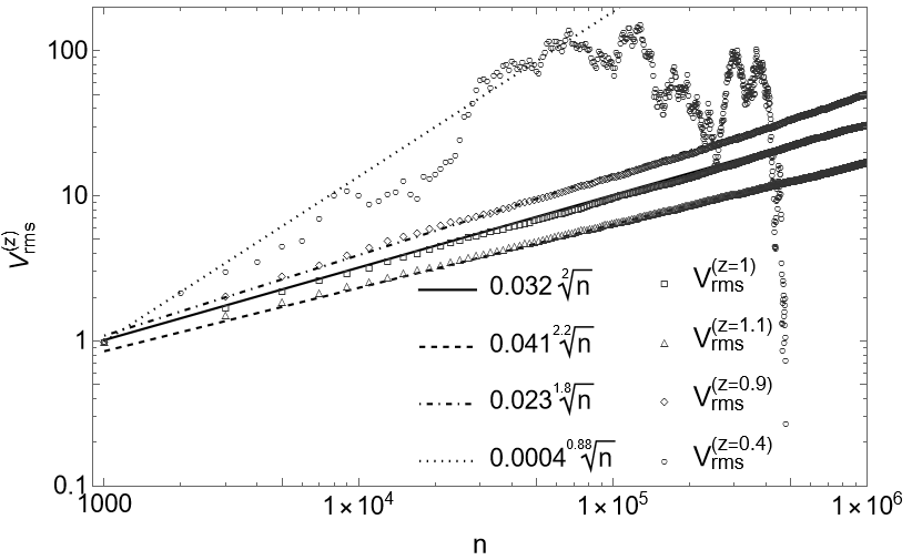
Figure 1: Vrms plots for 4 different values of $z$, considering an ensemble of $10^{4}$ initial conditions varying $\phi$ in the interval $[0,2\pi]$ and evolving $10^{6}$ iterations. For a better comparison between the graphs, a normalization was introduced such that $V_{rms}^{(z)}(1000)=1$ for any $z$ value. This normalization facilitates a more effective comparison of the $V_{rms}^{(z)}$ behaviors across different diffusive regimes. The iterations are conducted using $\gamma=1$,$\bar{\zeta}=5$, $z=1.1,\,1.0,\,0.9$, and $0.4$. The solid, dashed, dot-dashed and dotted lines represent the theoretical results represented by Eq (7).

To substantiate this behavior, we conducted numerical simulations with $n=10^{6}$ iterations and $10^{4}$ different initial conditions, for four different values of the parameter $z$: specifically, $z=1$, $z=1.1$, $z=0.9$, and $z=0.4$. According to Eq. (7), the anticipated results are as follows: for $z=1$, the result is$\sqrt[2z]{n}=n^{1/2}$; for $z=1.1$, the result is $\sqrt[2z]{n}=n^{1/2.2}$; for $z=0.9$, the result is $\sqrt[2z]{n}=n^{1/1.8}$; and for$z=0.4$, the result is $\sqrt[2z]{n}=n^{1/0.8}$. The numerical results obtained using Map (4), with the values of the $\gamma$ and $\bar{\zeta}$ parameters set to 1 and 5, respectively, are illustrated in Figure 1, alongside the power functions that fit the data. The number of iterations ($n=10^{6}$ ) ensures that the simulations capture the long-term behavior of the system, thereby providing a comprehensive understanding of the diffusion processes. Additionally, using $10^{4}$ different initial conditions allows us to account for variability and ensures that the results are not dependent on any specific starting point, thereby enhancing the robustness and generalizability of our findings. The numerical findings corroborate the theoretical results for the initial three cases, $z=1,\,1.1$ and $0.9$. However, for $z=0.4$, $V_{rms}^{(z)}$ initially exhibits diffusive behavior, approximately aligning with the theoretically predicted result. Yet, for larger iteration values $(n>10^{5})$, $V_{rms}^{(z)}$ abruptly approaches zero, indicating a dissipative process.

To elucidate this final outcome, Figure 2 presents a graph depicting $V_{rms}^{(z)}$ at the $10^{6}$th iteration, which we shall hereafter refer to as $V_{rms-\infty}^{(z)}$, as a function of $z$.

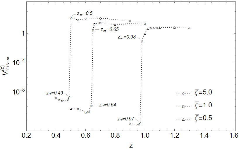
Figure 2: Graphs illustrating transition regions between the frozen phase and the diffusive phase for three distinct values of zeta. The critical values of z at which these transitions occur are emphasized.

It is clearly observed that, for a given $\bar{\zeta}$, there exists a critical value for $z$, below which $V_{rms-\infty}^{(z)}$ tends towards zero ($V_{rms-\infty}^{(z)}<10^{-8}$). This behavior can be interpreted as a "freezing" of the particle system, where the particles lose their dynamic motion and the system reaches a static state. In the notation used in the graph, $z_{\infty}$ represents the smallest value of $z$ that still permits diffusive processes. Conversely, $z_{0}$ represents the threshold value at which the system transitions into the frozen phase. The critical value $z_{\infty}$ serves as a point distinguishing between diffusive behavior and the frozen phase, thereby providing significant insight into the underlying dynamics of the system. The graph illustrates the range of $z$ values within which freezing occurs. For instance, when $\bar{\zeta}=5$, the value of $z$ that still permits diffusive states is $z_{\infty}=0.50$. If this value is decreased to $z_{0}=0.49$, the system transitions to the frozen state. Thus, a mere change of 0.01 in the $z$ value significantly alters the system’s behavior. For $\bar{\zeta}=0.3$, the limiting value of $z_{\infty}$ for the occurrence of diffusive states approaches 1.

These results can be further explored by developing a phase diagram that clarifies the relationship between the system’s behavior and the parameters $\bar{\zeta}$ and $z$. This process entails generating a grid of discrete points, with $\bar{\zeta}$ values ranging from 0.2 to 5 and $z$ values extending from 0.2 to 1.2. For each unique pair $(\bar{\zeta},z)$ within this grid, we compute the $V_{rms}^{(z)}$. Inspired by Eq. (1), we model the growth of $V_{\text{rms}}$ as a power-law function of $n$ (the number of iterations), expressed as $V_{\text{rms}}=an^{b}$. The resultant $V_{rms}^{(z)}$ values are subsequently categorized according to the exponent $b$, which provides insight into the diffusion behavior of the system. Specifically, for $b<0.49$, the system is classified as exhibiting subdiffusive behavior, indicating slower-than-normal diffusion. In the range $0.49<b<0.51$, the system demonstrates standard diffusive characteristics, where the diffusion process is characterized by a linear relationship with time. Conversely, for $b>0.51$, the system is classified as superdiffusive, suggesting a diffusion process that occurs at a rate faster than that of standard diffusion.

These classifications and their corresponding behaviors are illustrated in the accompanying Figure 3, which visually represents the varying diffusion regimes as a function of the parameters $\zeta$ and $z$.

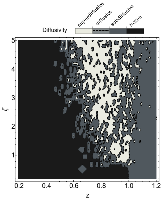
Figure 3: Phase diagram categorized by the power-law relationship $V_{\text{rms}}=an^{b}$. For $b<0.49$, the process is identified as subdiffusive, while for $b>0.51$, it is classified as superdiffusive. The boundary between these two regimes, where $0.49<b<0.51$, corresponds to a normal diffusion process.

Given that normal diffusive behavior is confined to a narrow range of $b$ values, it is represented by dashed lines at the boundaries between subdiffusive (light region) and superdiffusive regimes (gray region). The dark region represents the frozen phase.

For a complete analysis of this phase diagram, we will examine the dimensionality of the normal diffusion boundary that separates subdiffusive from superdiffusive behavior. For this we use the Box-Counting Method, also known as the Minkowski-Bouligand Dimension (Peitgen et al., 2004), is a common technique used to estimate the fractal dimension of a set. This method involves covering the set with a grid of boxes of size $\epsilon$ and determining how the number of boxes $N(\epsilon)$ that contain part of the set scales as the box size $\epsilon$ decreases.

The dimension $D$ is defined by the scaling relation:

$$D=\lim_{\epsilon\to 0}\frac{\log N(\epsilon)}{\log(1/\epsilon)}$$

In practice, we compute $N(\epsilon)$ for several values of $\epsilon$ and estimate the slope of the log-log plot of $N(\epsilon)$ versus $1/\epsilon$. This slope corresponds to the fractal dimension $D$. For the set of points defining the normal diffusive boundary, we determine the following dimensional value: $D=1.52439$. This result suggests the fractal nature of the boundary in question.

Therefore, the adiabatic parameter $z$ plays a crucial role in determining the dynamic behavior of the system. As $z$ varies, the system can transition from superdiffusive processes to normal diffusion, and ultimately to subdiffusive processes. We observe that within any diffusive regime, there is an unlimited increase in energy, a phenomenon referred to as Fermi acceleration. Furthermore, if the z parameter falls below a certain threshold, the system undergoes a “phase transition”, resulting in a "frozen" state. This indicates a rich structural complexity influenced significantly by variations in the $z$ parameter. To gain a deeper understanding of these results, it is essential to study the stability and chaos within this system.

IV Chaotic properties

The primary objective of this section is to examine the chaotic properties of the mapping to understand the transitions between diffusion regimes and the evolution of chaos during this process. Specifically, we aim to analyze how changes in key parameters influence the system’s behavior and the structure of its phase space.

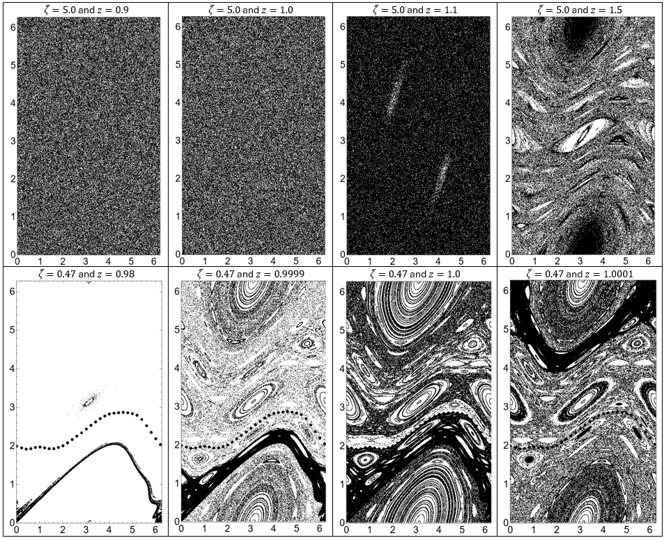
Figure 4: Phase spaces for various values of $\zeta$ and $z$. In all graphs, the x-axis corresponds to $\phi$, while the y-axis corresponds to $V$. The initial 200,000 data points are excluded to eliminate any transient states. In the first row, phase spaces corresponding to $\bar{\zeta}=5$ are shown, with $z$ varying from 0.9 to 1.5. The second row illustrates additional phase spaces for $\bar{\zeta}=0.47$, with $z$ exhibiting small variations in the range from 0.98 to 1.0001. It is important to note that the phase spaces with $z=1$ represents the established results for the standard map.

IV.1 Phase space

The phase space for map (4) is dependent on the value of the $\bar{\zeta}$ parameter as well as the adiabatic parameter $z$. Variations in these parameters result in significant changes to the phase space structure, which can provide insights into the underlying dynamics of the system. By systematically altering the $\zeta$ parameter and $z$, we can observe how the mapping transitions between different diffusion regimes, offering a deeper understanding of the interplay between order and chaos in the system. The resulting phase space structures are presented in Figure 4. The figure presents two graph lines, each characterized by a significantly different $\bar{\zeta}$ value. The first row illustrates the phase spaces for $\bar{\zeta}=5$ with $z=0.9$, $z=1.0$, $z=1.1$, and $z=1.5$. The $\bar{\zeta}$ value and corresponding $z$ values are selected to facilitate comparison with the $V_{rms}$ results depicted in Figure 1. A significant difference between the phase spaces for $z=0.9$ and $z=1.0$ is not readily observable. However, it is important to note that the former represents a superdiffusive process, while the latter corresponds to a diffusive process. The distinction between these diffusive processes will be more precisely identified by evaluating the evolution of the distance between two points in phase space through the calculation of Lyapunov coefficients. This method allows for a quantitative analysis of the system’s sensitivity to initial conditions, thereby providing deeper insight into the underlying dynamics of the diffusive and superdiffusive processes. By examining how these distances change over time, the Lyapunov coefficients serve as a critical tool in differentiating the behavior and stability of the processes in question.

Diffusive processes predominantly occur for $\zeta=5$, while "freezing" phenomena are observed in the second row for $z$ values below the threshold $z=0.98$. In the phase spaces depicted in the first row, the presence of chaos is evident, leading to superdiffusive processes for $z<1$ (e.g., $z=0.9$) and diffusive processes for $z=1$. For $z>1$, stable structures emerge within the phase space, which are expected to retard the increase in particle velocity, resulting in subdiffusive processes.

The second row presents the phase spaces for $\bar{\zeta}=0.47$ with $z=0.98$, $z=0.9999$, $z=1.0$, and $z=1.0001$. The chosen value for $\bar{\zeta}$ was inspired by the $K$ value for the standard map that still exhibits the last spanning invariant curve. In the standard map, the last spanning invariant curve is destroyed when the value of $K$ exceeds the critical value $K_{c}=0.9716\ldots$. In this scenario, local chaos, with $K<K_{c}$, transitions to global chaos when $K\geqslant K_{c}$ and the last invariant spanning curve is destroyed. In the model under consideration, the standard map is recovered when $z=1$. Therefore, in accordance with Eq.(5), we obtain a critical value for $\bar{\zeta}$:

$$\bar{\zeta}_{c}=\frac{K_{c}}{2}=0.4858...$$

By selecting $\zeta=0.47$, it is ensured that when $z=1$, the invariant spanning curve remains present in the phase space, as illustrated in the third graph of the second row in Figure 4. The sequence of black points represents the last spanning invariant curve. It should be noted that the invariant curve is, in fact, a continuous set of points, not a discrete one. This graphical representation using a discrete set is employed to illustrate where the last invariant curve would lie. In the case of the standard map, $z=1$, any initial condition placed at any point on the line will evolve along the line. However, with a variation of the $z$ value by one part in ten thousand, the invariant curve is transformed into an invariant region. In this context, the term "invariant region" refers to the phenomenon where, if any point on the original invariant curve is selected as the initial condition, this point evolves into a location within the dark regions, characterized by higher point densities, as highlighted in the graphs. Once the point reaches these regions, it becomes trapped within them, a property that was tested for up to $10^{8}$ iterations. So, in our simulations, we observed that these trajectories did not exhibit the stickiness phenomenon.

The system can be classified as a non-twist map, as it satisfies the condition where $\phi_{n}$ and $V_{n}$ are related by the equation $2^{z}\bar{\zeta}(z-1)\sin(\phi_{n})=V_{n}^{z}$, when $z\neq 1$. Consequently, we observe that

$$\frac{\partial\phi_{n+1}}{\partial V_{n}}=\gamma\left(1+(1-z)\frac{2^{z}\bar{\zeta}}{V_{n}^{z}}\sin(\phi_{n})\right)=0$$

violating the twist condition $\partial\phi_{n+1}/\partial V_{n}\neq 0$ (Reichl, 2004), which is a crucial statement for KAM’s theorem applicability to the map. So, The absence of shear (or twist) renders the system’s behavior less predictable, frequently resulting in complex dynamics, such as the formation of transport barriers, as observed in our simulations. Hence, when $z$ deviates from 1, the system undergoes a transition from a twist map to a non-twist map.

It is important to note that when $z<1$ is selected, the invariant curve is shifted to an invariant region below its original position, while for $z>1$, the corresponding invariant region is located above the initial position of the invariant curve. These observations can be seen in the phase spaces presented in the bottom row of graphs in Figure 4. The invariant curve is included in all phase spaces to facilitate the observation of these phenomena. However, it should be emphasized that in graphs where $z\neq 1$, the curve is no longer present.

When the adiabatic factor $z$ is reduced, the invariant region diminishes proportionally until reaching a threshold at $z=0.98$. For values of $z$ below this threshold, a transition to the frozen state occurs, resulting in the phase space becoming vacant.

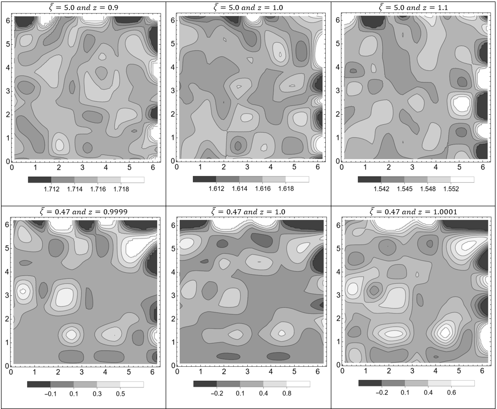
Figure 5: Variations in the values of the Lyapunov coefficients as a function of the $\bar{\zeta}$ and $z$ parameters. In all graphs, the coordinate axes depict the initial conditions. The initial phase $(\phi_{in})$ and initial velocity $(V_{in})$ are represented on the $x$-axis and $y$-axis, respectively. The grayscale bar denotes the values of the Lyapunov exponents.

IV.2 Jacobian determinant and Lyapunov coefficients

In the analysis of the dynamics of the mapping described in Eq (4), we observe that both chaotic and regular motion can coexist within the phase space (Fig. 4). This coexistence creates a scenario where there are significant variations and regions of local instability along any given chaotic trajectory. Essentially, the system does not follow a single predictable path but instead displays a complex interplay between different types of motion. The Jacobian determinant is given by

$$\det[J]=1+(1-z)\frac{\bar{\zeta}}{V_{n}^{z}}\cos\left(2V_{n}+\phi_{n}\right).$$

When $z\neq 1,$ $\det[J]$ has the possibility of being different from 1, suggesting that the system either expands or contracts the local phase space volume, indicating the presence of chaotic behavior, dissipation, or other complex dynamical phenomena.

The large variations in behavior are directly related to the system switching between distinct states of motion. Specifically, we see alternations between chaotic motion, where the system’s behavior is highly sensitive to initial conditions and appears disordered, and quasiregular motion, where the system shows more predictable, though not entirely regular patterns. This mix of behaviors within the same system introduces a layer of complexity that makes the dynamics particularly interesting and challenging to analyze.

To effectively characterize and understand these unique dynamic variations, we analyze the Lyapunov coefficients along some trajectories, which allows us to capture the intricate details of this modified standard map dynamics and better understand the interplay between the various diffusives regimes. The Lyapunov exponents for bidimensional systems are defined as (Eckmann and Ruelle, 1985)

$$\lambda_{j}=\lim_{N\rightarrow\infty}\frac{1}{N}\ln\left|\Lambda_{j}^{N}\right|$$

where $\Lambda_{j}^{N}$ are the eigenvalues of the matrix $M=\prod_{n=1}^{N}J(V_{n},\phi_{n})$ and $J$ is the Jacobian matrix evaluated over the orbit. The results are illustrated in Figure 5. In constructing this figure, the initial conditions were systematically chosen from an equally spaced grid of points, where the variables $V_{\text{in}}$ and $\phi_{\text{in}}$ were sampled within the interval $[0,2\pi]$. Subsequently, an iterative process was applied, extending over 1 million terms to ensure the accuracy and stability of the results.

In the first row of graphs, where $\zeta=5$, it is observed that as the value of $z$ increases, the average value of the Lyapunov exponents decreases. This trend indicates a transition in the system’s behavior: initially, it exhibits superdiffusive dynamics, then passes through a regime of normal diffusion, and eventually becomes subdiffusive. This observation aligns with the interpretation of Lyapunov exponents as indicators of the divergence of trajectories in phase space. A higher Lyapunov exponent corresponds to a faster rate of separation between trajectories, which is associated with a more diffusive behavior of the system.

IV.3 Transport properties

In the preceding sections, we examined the transition from a twist map to a non-twist map. Nevertheless, even after the disruption of the final invariant curve, an effective transport barrier may persist in phase space, contingent upon the system’s parameters. To account for this phenomenon, we calculate the ratio of the number of orbits that traverse the barrier to the total number of orbits, similarly to what was done in Ref. (Grime et al., 2023). Initially, we examine a set of conditions by fixing $V_{in}=1$ while varying $\phi_{in}$between 0.5 and 6.0. Through an iterative process consisting of $N=10^{5}$ steps, we determine the fraction of orbits that reach the points defined by $V_{N}$=2.6, corresponding to the maximum value attained by the last invariant spanning curve. The results are presented in Fig. 6. The bar with a grayscale represents the fraction of orbits that pass the barrier. In the black regions, this fraction of orbits is zero, that is, the system has a total barrier. It is noteworthy that when $z>1$, transmission occurs almost invariably, irrespective of the value of $\zeta$.

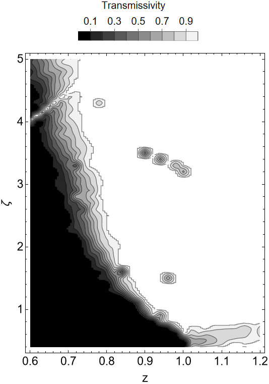
Figure 6: Transmissivity diagram. Fraction of orbits that reach or exceed the position of the maximum value reached by the last invariant spanning curve. The grayscale bar indicates the percentage of transmissivity.

This behavior can also be understood in the phase space diagrams in the second row of Figure 4, where it is apparent that the region with a higher density of points progressively shifts to higher values of $V$ as $z$ increases. This shift indicates that orbits, which were previously obstructed, encounter decreasing resistance, leading to a more extensive accessible region.

On the other hand, when $\bar{\zeta}$ assumes higher values, the system experiences an increase in chaotic dynamics, which facilitates greater transmissivity in phase space. In this context, transmissivity refers to the ability of orbits to traverse through phase space regions that might otherwise be obstructed. The increased chaos disrupts the regularity of the system, allowing orbits to pass through regions that would typically impede their progress.

The interface region, which lies between the zones of total blocking and the onset of transmissivity, exhibits fluctuations. These fluctuations are linked to variations in the local stability of the system, suggesting that small changes in stability can lead to significant differences in the behavior of orbits at this critical boundary. This behavior underscores the complex interplay between stability, chaos, and orbit dynamics within the system.

In graph of Figure 6, a clear qualitative similarity to graph of Figure 3 is observed, indicating that the overall behavior of the system remains consistent across both representations. Specifically, the freezing region in Figure 3 corresponds to the proportion of orbits that fail to overcome the established barrier. This region visually demonstrates where the system encounters resistance, leading to the trapping of orbits within a specific range of values of $\bar{\zeta}$ and $z$.

In addition to the freezing region, the other regions in graph of Figure 6 exhibit analogous behavior to those in graph of Figure 3. These regions reflect the varying capacities of the orbits to either escape or remain confined by the system’s underlying constraints.

V Conclusions and outlook

In this work, we analyzed the behavior of a boucing ball under the influence of an adiabatic parameter, which governs the energy transfer during each collision. The results demonstrate that the adiabatic parameter not only controls the energy exchange, where the particle may either gain or lose energy through an oscillatory interaction, but also fundamentally alters the structure and dynamics of the particle’s phase space.

The variation of the adiabatic parameter introduces a diverse range of dynamical regimes. For certain values, the particle can reach a "frozen" state, characterized by zero velocity ($V_{N}=0$), where the system appears to settle into a static configuration. In contrast, other regions of the parameter space lead to diffusive behaviors, with the particle exhibiting either subdiffusive or superdiffusive motion. The boundary between these diffusive regimes possesses fractal properties, reflecting the intricate, self-similar structure of phase space and indicating a sensitive dependence on initial conditions and parameter choices.

Moreover, the phase space is revealed to be mixed in nature, combining regions of regular motion with chaotic zones. This is confirmed by calculating the Lyapunov exponents, which indicate the presence of both chaotic and regular dynamics. In regions where the Lyapunov exponents are positive, the system exhibits chaotic behavior, characterized by sensitivity to initial conditions and exponential divergence of nearby trajectories. Conversely, regions with negative Lyapunov exponents suggest stable, predictable motion, marking a clear distinction between ordered and chaotic dynamics within the system. The presence of both positive and negative Lyapunov exponents underscores the mixed-phase nature of the system, with pockets of chaotic motion interspersed with stable, regular regions.

Furthermore, the variation of the adiabatic parameter induces a transition from a twist to a non-twist system. In classical twist systems, there is a systematic, predictable progression of orbits in phase space, but as the system shifts to a non-twist configuration, this order breaks down. This transition suggests the breakdown of the KAM tori and a fundamental change in the system’s topological properties, further contributing to the richness of the dynamical behavior.

Finally, we evaluated the transmissivity of the particle across the phase space. Our findings indicate that depending on the specific choice of parameters, the phase space can either be fully accessible, allowing the particle to explore the entire space, or partially accessible, where certain regions become dynamically inaccessible. This restricted access in certain parameter regimes introduces barriers in phase space, confining the motion of the particle and limiting the range of possible dynamical outcomes.

In conclusion, the interplay between the adiabatic parameter and the particle’s dynamics creates a complex and rich system, where energy exchange mechanisms, diffusive behaviors, chaotic and regular dynamics, and the twist-to-non-twist transition all contribute to a highly structured phase space. The study provides insights into how sensitive control parameters can significantly alter the global and local dynamics of a system, with implications for understanding similar phenomena in other physical systems governed by adiabatic processes.

The ongoing research aims to further develop the study by establishing a connection with thermodynamics. This is being achieved through the formal definition and analysis of the system’s entropy, which is expected to offer a physical perspective on the model. By integrating the concept of entropy, the study aims to enhance the theoretical framework and offer new insights into the behavior of the system under thermodynamic conditions.

Appendix A Anomalous Distribution

Considering the Gaussian form of normal diffusion, with an anomalous diffusion, we make a scaling hypothesis (Cecconi et al., 2022) so that we can express the anomalous distribution as

$$\Psi_{\mu}(V,n)=\sqrt{\frac{a}{\pi}}\frac{1}{n^{\mu}}\exp\left[-a\left(\frac{V}{n^{\mu}}\right)^{2}\right].$$ (8)

The associated moments are obtained as

$$\left\langle V_{n}^{2}\right\rangle = \intop_{-\infty}^{\infty}V^{2}\Psi_{\mu}(V,n)\,dV=\frac{n^{2\mu}}{2\sqrt{a^{2}}}.$$

$$\left\langle V_{n}^{2-2z}\right\rangle = \intop_{-\infty}^{\infty}V^{2-2z}\Psi_{\mu}(V,n)\,dV$$

$$= \frac{1}{\sqrt{a^{2-2z}\pi}}\varGamma\left(\frac{3-2z}{2}\right)\left(n^{2\mu}\right)^{1-z}.$$

So we can conclude that

$$\left\langle V_{n}^{2-2z}\right\rangle=\frac{2^{1-z}}{\sqrt{\pi}}\varGamma\left(\frac{3}{2}-z\right)\left\langle V_{n}^{2}\right\rangle^{1-z}.$$

Under this assumption, we can set $\left\langle V_{n}^{2-2z}\right\rangle=\alpha\left\langle V_{n}^{2}\right\rangle^{1-z}$, where $\alpha=\frac{2^{1-z}}{\sqrt{\pi}}\varGamma\left(\frac{3}{2}-z\right)$.

—————–

References

- Cussler (2009) E. L. Cussler, Diffusion (Cambridge University Press, 2009).
- Saxton (2001) M. J. Saxton, Biophysical Journal 81, 2226 (2001), ISSN 0006-3495.
- Geisel et al. (1985) T. Geisel, J. Nierwetberg, and A. Zacherl, Physical Review Letters 54, 616 (1985), ISSN 0031-9007.
- Szymanski and Weiss (2009) J. Szymanski and M. Weiss, Physical Review Letters 103, 038102 (2009), ISSN 0031-9007.
- Crank (1981) J. Crank, Diffusion in polymers (Academic Press, London [u.a.], 1981), 4th ed.
- Zwanzig (2001) R. Zwanzig, Nonequilibrium statistical mechanics (2001), URL http://search.ebscohost.com/login.aspx?direct=true&scope=site&db=nlebk&db=nlabk&AN=169150.
- Atkins (2018) P. Atkins, Atkins’ physical chemistry (Oxford University Press, Oxford, 2018), eleventh edition ed., ISBN 9780198769866.
- Alberts et al. (2007) B. Alberts, A. Johnson, J. Lewis, M. Raff, K. Roberts, and P. Walter, Molecular Biology of the Cell (W.W. Norton & Company, 2007).
- Pathria (2022) R. K. Pathria, Statistical mechanics (Academic Press, an imprint of Elsevier, London, 2022), fourth edition ed., ISBN 9780081026922, URL https://ui.adsabs.harvard.edu/abs/2022stme.book.....P.
- Huang (1987) K. Huang, Statistical Mechanics, 2nd Edition (1987), URL https://ui.adsabs.harvard.edu/abs/1987stme.book.....H.
- Chirikov (1979) B. V. Chirikov, Physics Reports 52, 263 (1979), ISSN 0370-1573.
- Lichtenberg and Lieberman (1992) A. J. Lichtenberg and M. A. Lieberman, Regular and Chaotic Dynamics (Springer New York, 1992), ISBN 9781475721843.
- Livorati et al. (2012) A. L. P. Livorati, T. Kroetz, C. P. Dettmann, I. L. Caldas, and E. D. Leonel, Physical Review E 86 (2012), ISSN 1539-3755.
- Chastaing et al. (2015) J.-Y. Chastaing, E. Bertin, and J.-C. Géminard, Am. J. Phys. 83, 518 (2015) 83, 518 (2015), ISSN 1943-2909, eprint 1405.3482.
- Liang and Lan (2010) S.-N. Liang and B. L. Lan, in Chaotic Systems (WORLD SCIENTIFIC, 2010), pp. 165–169.
- Boscolo et al. (2023) A. L. Boscolo, V. B. d. S. Junior, and L. A. Barreiro, Physical Review E 107, 045001 (2023), ISSN 2470-0053.
- Fermi (1949) E. Fermi, Physical Review 75, 1169 (1949), ISSN 0031-899X.
- Cecconi et al. (2022) F. Cecconi, G. Costantini, A. Taloni, and A. Vulpiani, Physical Review Research 4, 023192 (2022), eprint 2206.06786, URL https://ui.adsabs.harvard.edu/abs/2022PhRvR...4b3192C.
- Peitgen et al. (2004) H. Peitgen, H. Jürgens, and D. Saupe, Chaos and fractals - new frontiers of science (2. ed.) (Springer, 2004), ISBN 978-0-387-20229-7.
- Reichl (2004) L. E. Reichl, The Transition to Chaos (Springer New York, 2004), ISBN 9781475743500.
- Eckmann and Ruelle (1985) J. P. Eckmann and D. Ruelle, Reviews of Modern Physics 57, 617 (1985), ISSN 0034-6861.
- Grime et al. (2023) G. C. Grime, M. Roberto, R. L. Viana, Y. Elskens, and I. L. Caldas, Chaos, Solitons Fractals 172, 113606 (2023), ISSN 0960-0779.