Deep Equilibrium Algorithmic Reasoning

Abstract

Neural Algorithmic Reasoning (NAR) research has demonstrated that graph neural networks (GNNs) could learn to execute classical algorithms. However, most previous approaches have always used a recurrent architecture, where each iteration of the GNN matches an iteration of the algorithm. In this paper we study neurally solving algorithms from a different perspective: since the algorithm’s solution is often an equilibrium, it is possible to find the solution directly by solving an equilibrium equation. Our approach requires no information on the ground-truth number of steps of the algorithm, both during train and test time. Furthermore, the proposed method improves the performance of GNNs on executing algorithms and is a step towards speeding up existing NAR models. Our empirical evidence, leveraging algorithms from the CLRS-30 benchmark, validates that one can train a network to solve algorithmic problems by directly finding the equilibrium. We discuss the practical implementation of such models and propose regularisations to improve the performance of these equilibrium reasoners.

1 Introduction

Algorithms, while straightforward in theory, become challenging to deploy in real-world scenarios. They operate in abstract domains with very specific conditions and types of inputs, which are represented with scalars. The main hurdle is the need to “collapse” reality into a scalar every time an algorithm is used, something usually done based on intuition rather than principled science [25]. Neural Algorithmic Reasoning (NAR; 46) has been proposed to address this issue by utilising specialised neural network architectures to break this scalar bottleneck by executing algorithms in higher-dimensional space made out of arrays of numbers (vectors). The task of mapping reality into this vectorial space is delegated to automated gradient-based optimisation techniques rather than relying on human operators.

While NAR does not provide the correctness guarantees of its classical counterparts, robust performance can be achieved through alignment [55] – submodules of the model architecture correspond to easy-to-learn subparts of the algorithm (or class of). Graph Neural Networks (GNNs) have emerged as the most convenient architecture to execute all types of algorithms [29] and GNNs that align better to the target algorithm achieve better generalisation. This alignment game [50] has led to a sequence of exciting research – from aligning the architecture with iterative algorithms [42] to proving that “graph neural networks are dynamic programmers” [13], especially if their message-passing function [21] takes into account 3-node interactions.

The aforementioned papers focus on aligning the computation of the GNN with an algorithm or a specific algorithm class (e.g. dynamic programming), but ignore the properties at the time of algorithm termination. For the algorithms in the CLRS-30 algorithmic reasoning benchmark [45] once the optimal solution is found, further algorithm iterations will not change it. For example, in dynamic programming shortest-paths algorithms making additional iterations would not alter the optimality of the shortest paths’ distances found. Such a state is called an equilibrium – additional applications of a function (an algorithm’s iteration) to the state leave it unchanged.

In this paper:

1. We explore the connection between execution of algorithms and equilibrium finding through the use of Denotational semantics and Domain theory. (section 3)

2. Inspired by the above, we implement a class of deep equilibrium algorithmic reasoners (DEARs) that learn algorithms by identifying the equilibrium point of the GNN equation and propose improvements to them. (section 4)

3. Our results suggest that the above reasoners can be successfully trained. Not only does equilibrium algorithmic reasoning achieve better overall performance with less expressive (and expensive) GNNs, but is also competitive to the more expressive (and expensive) NAR models. All this is done without providing any information on the number of algorithmic steps – neither at train nor at test time. (section 5)

4. DEARs also drastically improve the inference speed – an achievement made possible by the use of optimised root-finding algorithms and by decoupling the neural model from the sequential implementation of algorithms in standard benchmark datasets. (section 5)

Related work

The main proposed application of NAR is settings where one wants to apply an algorithm, but it is impossible to represent reality with a single scalar, hence an “executor” operating in vector space and faithful to the algorithm is required [47, 50]. As NAR models are neural clones of algorithms, they need to provide correct output even for previously unobserved input sizes. Achieving robust out-of-distribution (OOD) generalisation is tricky. To this end a plethora of works have dedicated their attention to it – [42, 13, 8, 14] to name a few. Except for one concurrent work (a blog post;[53]), those works focus on improving the GNN step and many completely ignore the termination of algorithms or any properties of the last state, such as equilibrium. This work, similarly to Xhonneux et al., [53], studies neurally finding solutions to algorithms by relying on the equilibrium property. We, however, attempt to give the precise assumptions required for this approach to work. Further, we implement a more robust model than theirs, which achieves comparable or better performance to baselines. Finally, we propose modifications to improve equilibrium NARs.

2 Background

Algorithmic Reasoning

Let $A:{\mathbb{I}}_{A}\to{\mathbb{O}}_{A}$ be an algorithm, acting on some input ${\bm{x}}\in{\mathbb{I}}_{A}$, producing an output $A({\bm{x}})\in{\mathbb{O}}_{A}$ and let ${\mathbb{I}}_{A}$/${\mathbb{O}}_{A}$ be the set of possible inputs/outputs $A$ can read/return. In algorithmic reasoning, we aim to learn a function ${\mathcal{A}}:{\mathbb{I}}_{A}\to{\mathbb{O}}_{A}$, such that ${\mathcal{A}}\approx A$. Importantly, we will not be learning simply an input-output mapping, but we will aim to align to the algorithm $A$’s trajectory. The alignment is often achieved through direct supervision on the intermediate states of the algorithm. To capture the execution of $A$ on an input $x$ we can represent it as

$$\bar{{\bm{h}}}_{0}=\text{{Preproc}}({\bm{x}})$$ (1a) (1b) (1c)

where Preproc and Postproc are some simple pre- and post-processing (e.g.initialising auxiliary variables or returning the correct variable), $\bar{{\bm{h}}}_{\tau}\in{\mathbb{H}}_{A}$ is $A$’s internal (hidden) state, $A_{t}$ is a subroutine (or a set of) that is executed at each step and the number of steps depends on a boolean property being satisfied (e.g. all nodes visited). It is therefore no surprise that the encode-process-decode architecture [24] is the de-facto choice when it comes to NAR. Thus, the architecture can be neatly represented as a composition of three learnable components: ${\mathcal{A}}=g_{\mathcal{A}}\circ P\circ f_{\mathcal{A}}$, where $g_{\mathcal{A}}:{\mathbb{I}}_{A}\to{\mathbb{R}}^{d}$ and $f_{\mathcal{A}}:{\mathbb{R}}^{d}\to{\mathbb{O}}_{A}$ are the encoder and decoder function respectively (usually linear projections) and $P:{\mathbb{R}}^{d}\to{\mathbb{R}}^{d}$ is a processor that mimics the rollout (Equation 1b) of $A$. The processor often uses a message-passing GNN at its core.

CLRS-30

The CLRS-30 benchmark [45] includes 30 iconic algorithms from the Introduction to Algorithms textbook [11]. Each data instance for an algorithm $A$ is a graph annotated with features from different algorithm stages (input, output, and hint), each associated with a location (node, edge, and graph). Hints contain time series data representing the algorithm rollout and include a temporal dimension often used to infer the number of steps $\tau$. Features in CLRS-30 have various datatypes with associated losses for training. The test split, designed for assessing out-of-distribution (OOD) generalisation, comprises graphs four times larger than the training size.

Deep Equilibrium Models

Deep equilibrium models [DEQs 4] are a class of implicit neural networks [20]. The functions modelled with DEQs are of the form:

$${\bm{z}}^{*}=f_{\theta}({\bm{z}}^{*},{\bm{x}})$$ (2)

where ${\bm{x}}$ is input, $f_{\theta}$ is a function parametrised by $\theta$ (e.g. a neural network) and ${\bm{z}}^{*}$ is the output. ${\bm{z}}^{*}$ is an equilibrium point to the eventual output value of an infinite depth network where each layer’s weights are shared, i.e. $f_{\theta}^{[i]}=f_{\theta}$. By re-expressing (2) as $g_{\theta}=f_{\theta}({\bm{z}}^{*},{\bm{x}})-{\bm{z}}^{*}$ DEQs allow us to find the fixed point ${\bm{z}}^{*}$ via any black-box root-finding method [e.g. 9, 2], without the actual need to unroll the equation until convergence, allowing us to reduce steps. For backpropagation the gradient $\partial\mathcal{L}/\partial\theta$ could be calculated using the Implicit Function Theorem (cf. 4) and no intermediate state has to be stored, giving us a constant memory cost of gradient computation regardless of the number of iterations until convergence.

Expander graphs

MPNNs operate by exchanging information between adjacent nodes [21]. It has been identified that the message passing process can be hindered by a phenomenon known as oversquashing [1], which occurs when a large volume of messages are compressed into fixed-sized vectors. The importance of overcoming the negative implication posed by this phenomenon is crucial for the overall expressivity of GNNs [22], particularly in the context of long-range node interactions.

To this end, several spectral methods have been proposed to mitigate oversquashing by increasing the Cheeger constant [3, 6, 30]. A higher Cheeger constant provides a measurement that a graph is globally lacking bottlenecks. The novel approaches include graph rewiring techniques [44, 7], as well as significant independent bodies of research recognising the efficacy of expander graphs [12, 41, 6], due to their desirable properties.

Expander graphs are proven to be highly connected sparse graphs ($|E|=\mathcal{O}(|V|)$) with a low diameter [35], thus offering advantageous properties for information propagation. Consequently, this facilitates messages to be passed between any pair of nodes in a short number of hops, and as a result, alleviating oversquashing. Formally, a graph $G=(V,E)$ is defined as an expander if it satisfies certain expansion properties. One common definition involves the aforementioned Cheeger constant. In the work of Deac et al., [12], a high Cheeger constant is equivalent to a graph being bottleneck free [12, Definition 3], and that an expander has a high Cheeger constant [12, Theorem 5].

There are various methods for constructing expander graphs. We opt for the deterministic algebraic approach as in Deac et al., [12], utilising Cayley graphs. Specifically, we leverage Definition 8 and Theorem 9 of [12] to construct the Cayley graph for the special linear group $\mathrm{SL}(2,{\mathbb{Z}}_{n})$ and its generating set $S_{n}$ – see p.5 of Deac et al., [12] for details. Note, that the order of a Cayley graph for ${\mathbb{Z}}_{n}$ is $\left|V\right|=\mathcal{O}(n^{3})$. Hence, for many input graphs, a Cayley graph of the same size may not exist.

3 Denotational semantics: The denotation of a while loop statement

This aim of this section is to draw the parallel between finding equilibriums and executing an algorithm, in order to answer if and when an equilibrium NAR model can be successful. The following paragraphs introduce the mathematical tools for formalising fixed points – denotational semantics [39] and domain theory [38].

Denotational semantics

To every programming language expression $P$ denotational semantics provides an interpretation $\llbracket P\rrbracket$, which is a mathematical object (often a function), representing the behaviour of the expression to different inputs. These denotations must be: 1) abstract, i.e. independent of language and hardware, hence functions are natural choice; 2) compositional, i.e. $\llbracket P\rrbracket$ can only be defined in terms of the denotations of $P$’s subexpressions, but not $P$ itself; 3) model the computation $P$ performs. As an example, we will use the lightweight imperative programming language IMP. It consists of numbers, locations, arithmetic expressions, boolean expressions and commands. Examples of IMP are given in Appendix A – we will use blue for IMP and encourage the reader to check how we use colour in the appendix. Albeit small, the language is Turing-complete and all algorithms we experiment with can be defined in it.

Denote the set of variable locations with ${\mathbb{L}}$ – those are all variables/array elements we can ever define. A good analogy to think of is the addresses in the language C. The notation we can use to represent a program state is $[X\mapsto 1,B\mapsto-48,\dots]$ and means that the value of $X$ is 1, the value of $B$ is $-48$ and so on. In other words, program states map locations to integers, s.t. a location can be mapped only once. Hence states are functions and the set of all program states $State$ is the set of functions mapping locations to integers: given $s\in State$, $s(L)\in{\mathbb{Z}}$ is the value at the location $L$ for the state $s$. The value for location $L$ in a different $s^{\prime}\in State$, $s^{\prime}(L)$, may or may not differ. The denotation of arithmetic / boolean expressions / commands are the functions with domain $State$. These will be represented in the form of lambda abstractions, i.e. $\lambda x\in S.M$ rather than $f(x\in S)=M$, where $S$ is a set and $M$ is a function body. The codomain of the denotation depends on the type of expression: $\llbracket a\rrbracket:State\to{\mathbb{Z}}$ for arithmetic expressions, $\llbracket b\rrbracket:State\to{\mathbb{B}}$, for boolean expressions and $\llbracket c\rrbracket:State\rightharpoonup State$ for commands. Since commands transform state, they are also called state transformers. Commands’ denotations are partial functions, as expressions like while true do skip never terminate and have no denotation.

For a large portion of the above language, it is trivial and intuitive to define the denotations by structural recursion. For example:

$$\llbracket\texttt{{\color[rgb]{0.0600000000000001,0.46,1}if}}\ b\ \texttt{{\color[rgb]{0.0600000000000001,0.46,1}then}}\ c_{0}\ \texttt{{\color[rgb]{0.0600000000000001,0.46,1}else}}\ c_{1}\rrbracket=\lambda s\in State.\ \begin{cases}\llbracket c_{0}\rrbracket(s)\quad\text{if }\llbracket b\rrbracket(s)\text{ is {{\color[rgb]{0.0600000000000001,0.46,1}true}}}\\ \llbracket c_{1}\rrbracket(s)\quad\text{otherwise}\end{cases}$$

$$\llbracket\texttt{{\color[rgb]{0.0600000000000001,0.46,1}(}}c_{0}\texttt{{\color[rgb]{0.0600000000000001,0.46,1};}}c_{1}\texttt{{\color[rgb]{0.0600000000000001,0.46,1})}}\rrbracket =\lambda s\in State.\ \llbracket c_{1}\rrbracket(\llbracket c_{0}\rrbracket(s))\qquad\qquad\qquad\llbracket skip\rrbracket=\lambda s\in State.\ s$$

The only denotation that cannot be expressed recursively, is that of the while construct. Let $w=\texttt{{\color[rgb]{0.0600000000000001,0.46,1}while}}\ b\ \texttt{{\color[rgb]{0.0600000000000001,0.46,1}do}}\ c$. By program equivalence, $w=\texttt{{\color[rgb]{0.0600000000000001,0.46,1}if}}\ b\ \texttt{{\color[rgb]{0.0600000000000001,0.46,1}then}}\ \texttt{{\color[rgb]{0.0600000000000001,0.46,1}(}}c\texttt{{\color[rgb]{0.0600000000000001,0.46,1};}}w\texttt{{\color[rgb]{0.0600000000000001,0.46,1})}}\ \texttt{{\color[rgb]{0.0600000000000001,0.46,1}else skip}}$. Therefore

$${\color[rgb]{0.83984375,0.03125,0.23046875}\llbracket w\rrbracket}=\llbracket\texttt{{\color[rgb]{0.0600000000000001,0.46,1}if}}\ b\ \texttt{{\color[rgb]{0.0600000000000001,0.46,1}then}}\ \texttt{{\color[rgb]{0.0600000000000001,0.46,1}(}}c\texttt{{\color[rgb]{0.0600000000000001,0.46,1};}}w\texttt{{\color[rgb]{0.0600000000000001,0.46,1})}}\ \texttt{{\color[rgb]{0.0600000000000001,0.46,1}else skip}}\rrbracket =\lambda s\in State.\ \begin{cases}{\color[rgb]{0.83984375,0.03125,0.23046875}\llbracket w\rrbracket}\left(\llbracket c\rrbracket(s)\right)&\text{if }\llbracket b\rrbracket(s)\text{\ is {{\color[rgb]{0.0600000000000001,0.46,1}true}}}\\ s&\text{otherwise}\end{cases}$$

but this is not a valid definition, since it reuses $\llbracket w\rrbracket$ (highlighted in red above). Denotational semantics solves this problem, by defining a function $f_{b,c}:(State\rightharpoonup State)\to(State\rightharpoonup State)$ which takes one state transformer and returns another:

$$f_{b,c}=\lambda\hat{w}\in(State\rightharpoonup State).\lambda s\in State.\ \begin{cases}\hat{w}\left(c(s)\right)&\text{if }b(s)\\ s&\text{otherwise}\end{cases}$$ (3)

$\hat{w}$ is now a function variable. The denotation of $\llbracket w\rrbracket$ is the fixed point of $f_{\llbracket b\rrbracket,\llbracket c\rrbracket}$, i.e. $\llbracket w\rrbracket=f_{\llbracket b\rrbracket,\llbracket c\rrbracket}(\llbracket w\rrbracket)$. In order to find the denotation, we need to solve the fixed point. To aid the reader a full worked example of computing the denotation for a while loop construct is given in Appendix B.

Domain theory

Scott, [38] provides a framework with which we can both find and also characterise solutions for fixed point equations. Define $D$ as the domain of state transformers $(State\rightharpoonup State)$. A partial order $\sqsubseteq$ on $D$ is defined as follows: $w\sqsubseteq w^{\prime}$ iff $\forall s\in State$ if $w(s)$ is defined then $w(s)=w^{\prime}(s)$. In other words $w^{\prime}$ keeps old mappings and only defines new ones. The totally undefined partial function $\bot$ is the least element in $D$. This function contains no location to value mappings. A chain is a sequence of elements of $D$, s.t. $d_{0}\sqsubseteq d_{1}\sqsubseteq d_{2}\sqsubseteq\dots$ . The supremum of the chain, called least upper bound (lub), is denoted as $\bigsqcup_{n\geq 0}d_{n}$. There could exist different chains, but, by definition, all chains in a domain must have a lub.

A function $f:D\to D$ is monotonic iff $\forall d,d^{\prime}\in D.\ (d\sqsubseteq d^{\prime}\Rightarrow f(d)\sqsubseteq f(d^{\prime}))$. In other words, if the second state defined more mappings than the first and we apply one iteration step to both states, the state resulting from the second will still define more mappings. Monotonic functions for which $\bigsqcup_{n\geq 0}f(d_{n})=f(\bigsqcup_{n\geq 0}d_{n})$ are also called continuous. In plain language, if a function is continuous and we are provided with a chain, the lub of $f$ applied to every chain element is the same as $f$ applied to the lub of the chain. An element $d^{\prime\prime}\in D$ is defined to be pre-fixed point if $f(d^{\prime\prime})\sqsubseteq d^{\prime\prime}$ – applying $f$ does not define anything new. The fixed point $fix(f)$ of $f$ is the least pre-fixed point of $f$. By utilising antisymmetry of $\sqsubseteq$ and the two properties of $fix(f)$ (pre-fixed point and least) we can obtain $f(fix(f))=fix(f)$. By Tarski’s theorem [43], any continuous $f:D\to D$ has a least pre-fixed point. This fixed point can be found, by taking the lub of the chain of applications of f: $fix(f)=\bigsqcup_{n\geq 0}f^{n}(\bot)$. The helper function $f_{b,c}$ from Equation 3 is continuous [proof is given on p.120 of 23], therefore a direct result is that if the $\texttt{{\color[rgb]{0.0600000000000001,0.46,1}while}}\ b\ \texttt{{\color[rgb]{0.0600000000000001,0.46,1}do}}\ c$ terminates then its denotation exists and is the least fixed point of sequence of iterations (compared to picking any fixed point).

Denotational semantics and NAR

The above detour into denotational semantics has affirmed the existence of a connection between equilibrium models and algorithms (as conjectured by Xhonneux et al., [53]). Under the assumptions that:

• the algorithms always terminate – while not computable in the general case, this holds true for experiments, as we are dealing with offline algorithms with provable termination

• the algorithms we train on can be modelled as “$\texttt{{\color[rgb]{0.0600000000000001,0.46,1}while}}\ b\ \texttt{{\color[rgb]{0.0600000000000001,0.46,1}do}}\ c$” constructs within IMP

the least fixed point exists and can be found by taking the first “state” of the algorithm where future iterations on it have no effect. In Appendix C we have further annotated three algorithms from the official code of the CLRS benchmark: BFS, Floyd-Warshall, strongly connected components. Those annotations clearly show that algorithms can be rewritten in IMP regardless of their implementation size. While BFS is clearly a “$\texttt{{\color[rgb]{0.0600000000000001,0.46,1}while}}\ b\ \texttt{{\color[rgb]{0.0600000000000001,0.46,1}do}}\ c$”-type of algorithm, annotating the other two reveals that either the network may need more input features to decide termination (Floyd-Warshall; 2) or that the algorithm can be composed of several while loops where each $c$ is another while loop on its own (strongly connected components; 3). Fortunately, our approach is not doomed to fail: a single DEQ layer can model any number of “stacked” DEQ layers [32, chapter 4].

4 Deep equilibrium algorithmic reasoning

Architecture

We implement our processors/encoders/decoders following Ibarz et al., [29]. The most notable difference to their implementation is that ours uses a sparse graph representation. This requires us to assume a fully connected graph on tasks where no graph structure exists, in order to be able to give pointer predictions, and to reimplement the strongly connected components algorithm so that the output pointers are always in the edge set (this did not change the difficulty of the task).

The final node embeddings, from which the output is decoded, are the solution to the equation:

$$\begin{split}{\mathbf{H}}^{(*)}=P_{{\mathbf{U}}{\mathbf{E}}}({\mathbf{H}}^{(*)})\end{split}$$ (4)

where $P_{{\mathbf{U}}{\mathbf{E}}}({\mathbf{H}}^{(*)})=P({\mathbf{H}}^{(*)},{\mathbf{U}},{\mathbf{E}})$, ${\mathbf{U}}$/${\mathbf{E}}$ are the encoded node and edge feature matrices and $P$ is the processor function. ${\mathbf{H}}^{(t)}$ are the stacked latent states of the nodes at timestep $t$ (with ${\mathbf{H}}^{(0)}=\mathbf{0}$). The above Equation 4 matches the signature of Equation 2, and can be solved via root-finding (we employ torchdeq [19]; MIT License), as if it is $f_{\theta}$ of a DEQ. Any model using this technique will be called deep equilibrium algorithmic reasoner (DEAR) in our experiments. The default processor in the majority of our experiments is a PGN [48] with a gating mechanism as in Ibarz et al., [29], but we note that DEARs can use any kind of processor.

Finding the fixed point

The torchdeq library provides several solvers. The most basic one is fixed-point iteration, equivalent to repeating Equation 4 until convergence. However, in our very first experiments the solver needed more iterations than the algorithm we train on. We therefore opted for the Anderson solver (implements Anderson acceleration [2]) and abandoned fixed-point iteration:

$$\hat{{\mathbf{H}}}^{(t+1)}=P_{{\mathbf{U}}{\mathbf{E}}}({\mathbf{H}}^{(t)})\qquad{\mathbf{H}}^{(t+1)}=SolverStep\left(\left[{\mathbf{H}}^{(0)}\dots\mathbf{H}^{(t)}\right],\hat{{\mathbf{H}}}^{(t+1)}\right)$$

The criteria for pre-fixed point check torchdeq implements is distance-based: for a state ${\mathbf{H}}^{(t)}$ to be considered a pre-fixed point, the distance to the next state has to be under a pre-defined threshold $\delta$. We kept the criteria but modified the library to always return the least pre-fixed point (see Appendix E). This is in contrast to picking the pre-fixed point with the least distance to next state (the default option in torchdeq) and is a decision largely motivated from section 3. Due to a lack of a suitable definition for the domain of NAR trajectories, we define $\forall t.\ {\mathbf{H}}^{(t)}\sqsubseteq{\mathbf{H}}^{(t+1)}$, i.e. we pick the first state that passes the pre-fixed point check.

Globally propagating information

For problems defined on graphs it is in theory possible that the number of solver iterations needed to find equilibrium is less than the diameter of the graph. While, in practice, this is unlikely to happen we hypothesise that improving long-range interactions could improve the convergence of DEAR. For this reason, we adopt the implementation of Cayley Graph Propagation (CGP) [51]. Contrasted to Expander Graph Propagation (EGP) [12], which addresses the graph size misalignment (see section 2) by truncating the Cayley graph, CGP keeps the extra nodes as virtual nodes. The CGP model upholds the aforementioned advantageous properties of an expander graph in a more grounded manner by preserving the complete structure.

In GNNs, the benefits of augmenting a graph with virtual nodes and providing message-passing shortcuts have been observed to improve performance in various tasks [27, 26, 10]; further supported by the theoretical analysis [28]. Additionally, by retaining the complete Cayley graph structure we improve the structure-aware representations by varying the neighbourhood ranges [54].

No hint by default

We do not make any use of hints (supervising on intermediate algorithm state). First, although it may seem counterintuitive, it has been shown that a NAR model can successfully generalise, and even give better results when trained to only predict the correct output [8, 37]. Second, the fact that the solver uses the GNN exactly once per call does not imply that one step of the solver would correspond to one iteration of the algorithm, bringing uncertainty which DEAR states to match to which algorithm step. While we propose an alignment scheme (see next paragraph), which has the potential to integrate hints, we leave this for future work.

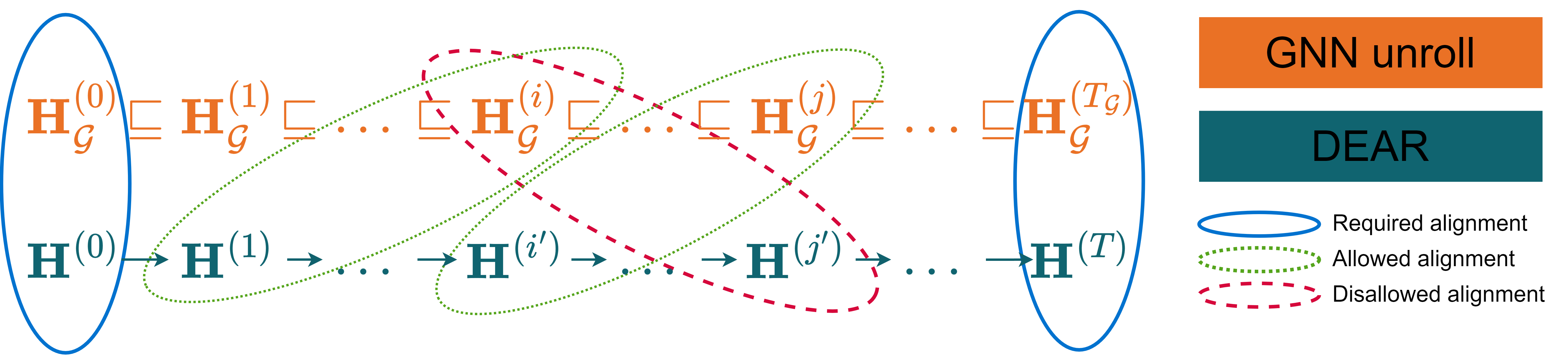
Figure 1: Proposed alignment rule: every state in the DEAR trajectory should “go forward”. Alignments to a GNN state that has already been “passed” are disallowed. First and last states must always align. We intentionally use arrows instead of $\sqsubseteq$ for DEAR, as $\sqsubseteq$ may not hold for DEAR’s trajectory.

Alignment

Our idea of alignment is visualised in Figure 1. We are given two trajectories of states, one obtained from unrolling GNN iterations as in classical NAR and another obtained from using DEAR. We would like to match DEAR to NAR, such that $\forall i\leq j,i^{\prime}\leq j^{\prime}$ if we have committed to aligning DEAR state ${\mathbf{H}}^{(i^{\prime})}$ to NAR state ${\mathbf{H}}^{(j)}_{\mathcal{G}}$, we cannot align any ${\mathbf{H}}^{(j^{\prime})}$ to ${\mathbf{H}}^{(i)}_{\mathcal{G}}$ and from the same start we would like to reach the same final state. In other words, skipping states is allowed, going back in time is not. This auxiliary supervision would also improve the monotonicity of DEARs, encouraging faster convergence. Enforcing this alignment is done by using an auxiliary loss. Choosing the $L_{2}$ norm as a distance metric, we use a dynamic programming algorithm (Appendix F) to compute the most optimal alignment (normalised by the number of solver steps, in order not to penalise longer trajectories) and supervise on that value.

Even with normalisation, the alignment sometimes had the effect of making the optimisation stuck in local minima where the number of steps to hit equilibrium was as low as 2 and the gradients were uninformative. We combated this in two ways: 1) instead of using the default layer normalisation we switched to granola [15]; 2) since $f(fix(f))=f$, we performed a random number of additional iterations [33] and take the last state. The probability of doing $s$ extra steps is $0.5^{s}$.

5 Evaluation

Setup

For each algorithm we generated $10^{5}$/100/100-sized training/validation/test datasets. Training sample sizes vary between 8 and 16 elements (uniformly randomly chosen) validation samples are of size 16. As is standard in NAR literature, we measure the test performance out-of-distribution, so our test samples are of size 64. For algorithms on graphs we generate Erdős–Rényi graphs [17] with edge probabilities $p$ uniformly sampled from the interval $[0.1,0.9]$, with increments of $0.1$, which is the data distribution our baselines [29, 8] have used. We obtained the ground truth execution trajectories and targets using the CLRS-30 implementation [45].

In our experiments the models have a latent dimensionality of 128, the batch size is 32, the learning rate is $3\times 10^{-4}$ and we use the Adam optimizer [31]. We train our algorithmic reasoners for 100 epochs, choosing the model with the lowest task validation loss (discounting any regularisation; focusing on performance only) for testing. Each task is independently learned, minimising the output loss (losses depend on the algorithm, cf. CLRS-30) plus any regularisation losses. Unless otherwise specified, DEARs employ the Anderson root-finding method from the torchdeq library and include Jacobian regularization [5], the tolerance for fixed point criteria on the forward pass is $\delta=0.1$ (and $\frac{\delta}{10}$ on the backwards) and is based on the relative $L^{2}$ norm between GNN states. Standard deviations are based on 3 seeds. If run on a single 4090 GPU one would need about 3 weeks of total compute.

Figure 2: Despite converging to slightly higher train loss our models remain stable during optimisation

Table 1: Test accuracy for different algorithms and models. Models with a diamond ($\lozenge$ or $\blacklozenge$) iterate for the correct amount of steps during train time (may differ between datapoints). Filled diamond ($\blacklozenge$) means the ground truth number of steps is also given at test time. LT stands for learnt termination – the model that uses a termination network. For DEM [53] we leave a $-$ when no results are reported and we report two results for shortest path and MST as it is unclear to us from the main text how they differentiated between the two. We do not run DEAR with CGP for array tasks as they operate on fully-connected graphs.

Algorithm	NAR◆	NAR◆ (Triplet-MPNN)	NAR◆ (LT)	DEM	DEAR (ours)	DEAR (with CGP; ours)
Weighted graphs
Bellman-F.	$97.06\%\pm 0.40$	$97.23\%\pm 0.15$	$95.39\%\pm 1.42$	$96.4\%$/$78.8\%$	$96.78\%\pm 0.43$	$94.23\%\pm 0.59$
Floyd-W.	$52.53\%\pm 0.98$	$61.86\%\pm 1.57$	$49.30\%\pm 0.53$	-	$55.75\%\pm 2.20$	$53.20\%\pm 2.45$
DSP	$94.21\%\pm 1.77$	$93.32\%\pm 1.60$	$88.30\%\pm 1.04$	-	$89.81\%\pm 0.14$	$89.49\%\pm 0.17$
MST Prim	$93.56\%\pm 0.77$	$92.01\%\pm 1.50$	$87.69\%\pm 1.17$	$82.3\%$/$75.2\%$	$88.67\%\pm 0.74$	$86.37\%\pm 0.36$
Unweighted graphs
BFS	$99.85\%\pm 0.09$	$99.69\%\pm 0.29$	$99.51\%\pm 0.06$	$53.8\%$	$98.73\%\pm 0.37$	$98.28\%\pm 0.55$
DFS	$16.89\%\pm 5.73$	$31.20\%\pm 4.02$	$29.07\%\pm 2.32$	5.0%	$40.62\%\pm 0.44$	$23.87\%\pm 2.49$
SCC	$40.70\%\pm 1.39$	$46.84\%\pm 1.70$	$39.33\%\pm 1.52$	-	$43.63\%\pm 1.19$	$38.71\%\pm 0.45$
Arrays (assumes fully-connected graph)
Search (Binary)	$94.67\%\pm 2.31$	$93.33\%\pm 2.31$	$84.33\%\pm 8.33$	-	$59.00\%\pm 12.3$	-
Minimum	$97.67\%\pm 5.73$	$96.67\%\pm 2.31$	$94.00\%\pm 2.00$	-	$97.22\%\pm 3.82$	-
Sort (Ins.)	$27.07\%\pm 10.3$	$63.67\%\pm 39.97$	$33.8\%\pm 12.04$	-	$86.93\%\pm 3.87$	-
Overall	$71.42\%$	$\mathbf{77.58\%}$	$70.07\%$	-	$75.42\%$	-

The performance metric we measure is the out-of-distribution accuracy, hence the larger test instances. The definition of accuracy varies between algorithms and is based on the specification of the algorithm itself. We refer the reader to Veličković et al., [45] and CLRS-30 for corresponding accuracy metrics definitions. The main baselines we compare against are the results reported by Xhonneux et al., [53], as no implementation is publicly available, and a NAR architecture with a PGN processor trained in the no-hint regime, as done by Bevilacqua et al., [8]. As, logically, models that are provided the ground-truth number of steps at test time will perform better, we also add as additional baselines a model that always uses 64 steps at test time and a model that has a dedicated network to decide termination [49]. In order to understand how we compare to other, architectural alignments, we also provide a comparison with a more expressive processor (Triplet-MPNN).

5.1 Results

We present results for 10 key algorithms (most of the ones used in Bevilacqua et al., [8]) in Table 1.

DEARs are reasoners

The first set of experiments aims to establish whether learning to execute algorithms by finding the least fixed point is possible. As Xhonneux et al., [53] report that their models were prone to optimisation issues, we first compared the training loss for a standard NAR model and a DEAR model with the same neural components. The plots are visualised in Figure 2. In line with the previous work, we observed that the DEAR tends to converge to a slightly higher training loss as no algorithm’s mean training loss dropped below 0.01. However, as evident in Figure 2, we found the optimisation to be overall stable, and the final train loss difference between NAR and DEAR was never greater than 0.1 – see Appendix G. We are unaware if Xhonneux et al., [53] observed the same numerical differences, but we were overall satisfied with the convergence of DEARs.

Equilibrium is a useful inductive bias

DEAR outperforms both of the above baselines achieving a 4-5% overall score increase, suggesting that aligning to the equilibrium property is a useful inductive bias. Moreover, DEAR with a PGN processor is comparable to a NAR with the more expressive Triplet-MPNN, achieving only 2% lower overall accuracy. This commendable achievement required no information about the ground-truth number of steps neither at train time nor during inference. A more detailed performance analysis follows.

On weighted graph algorithms our model performed on par with the baseline NAR no-hint model for Bellman-Ford, it outperformed the baseline on Floyd-Warshall, and scored slightly behind on the other two. On unweighted ones, it retained fairly high BFS accuracy compared to DEM and it provided better scores for DFS and Strongly Connected Components (SCC). Unfortunately, even though for this kind of algorithms we used separate edge features for the CGP, in order to distinguish CGP edges from input ones, CGP had a detrimental effect. We hypothesise that algorithms like DFS and SCC need a more advanced architecture or require different task specifications (the algorithm for SCC has a parallel “twin”; see [16]) in order to generalise OOD. On algorithms on arrays, we got a significant performance improvement in the sorting task and got almost equal scores for min finding. However, the model underperformed by a large margin on the binary search task (in red). This result was very concerning, so we investigated further – Appendix H showed that DEARs overfitted a lot on the classic representation of binary search and that when the task is designed carefully, DEARs can reach overall performance of a Triplet-MPNN NAR architecture.

Figure 3: Cayely graph propagation can help with convergence

Effects of using CGP

Despite the slightly lower accuracies, our experiments with CGP have not been futile. In Figure 3, we observe that for almost half of the algorithms CGP applies to, it had a positive effect on the loss convergence – 3/7 algorithms converged to at least half an order of magnitude lower train loss. The rest did not experience any strong negative effects of CGP. Per-algorithm plots can be found in Appendix I. We believe that the reduced accuracies are due to the nearest Cayley graph for the training sizes being unique and a size of 24 nodes. Our deterministic approach of generating a fixed Cayley graph for CGP, whose size is still distinct from test-time size leads to overfitting; what we may observe here. Future avenues of work may want to investigate this by methodically removing the Cayley graph’s edges, but still retaining the desirable expansion properties [6], or by exploring alternative novel graph wiring techniques [7]. However, the limitation of these proposed approaches in comparison to CGP is that they may require dedicated preprocessing to scale (one of the desirable criteria set by the EGP method), therefore providing an interesting line of future work.

Alignment can distill knowledge into DEARs

For evaluating our alignment we focused on the non-CGP version of DEAR and decided to pick algorithms where: 1) The baseline performs reasonably well (90+% accuracy), so as to provide good support; 2) the DEAR underperforms substantially. The algorithms to fulfil those requirements are: DAG Shortest paths, MST Prim and Binary Search.

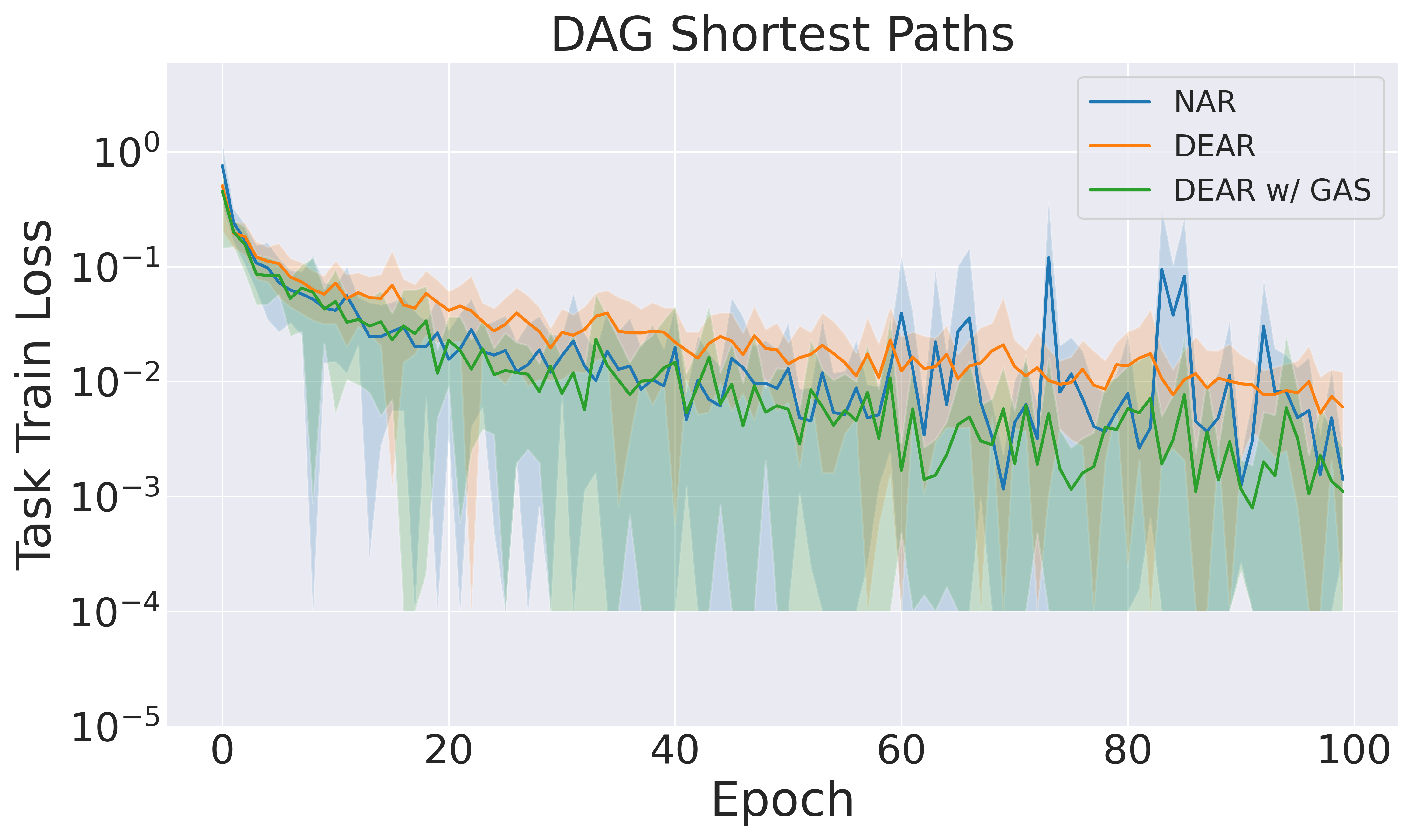
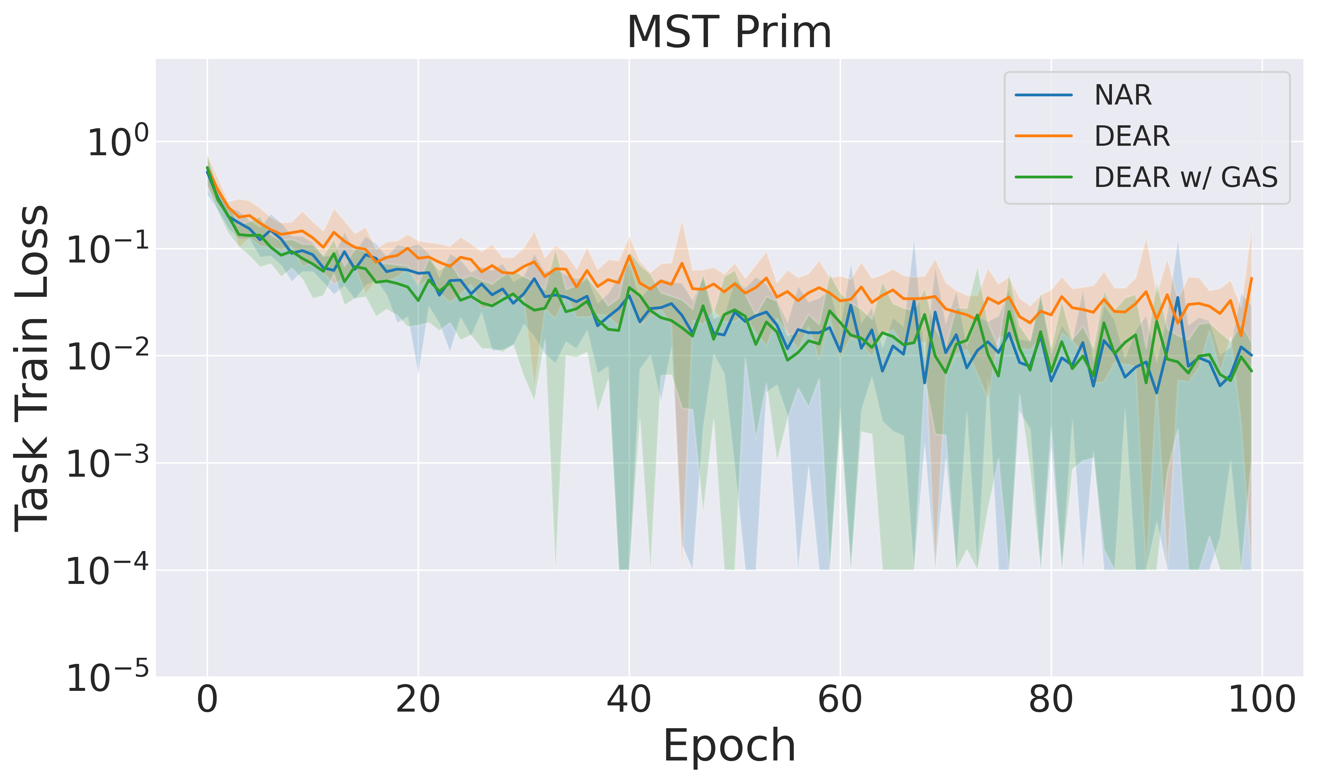
Figure 4: Alignment (with granola and stochasticity; DEAR w/ GAS) gives better convergence

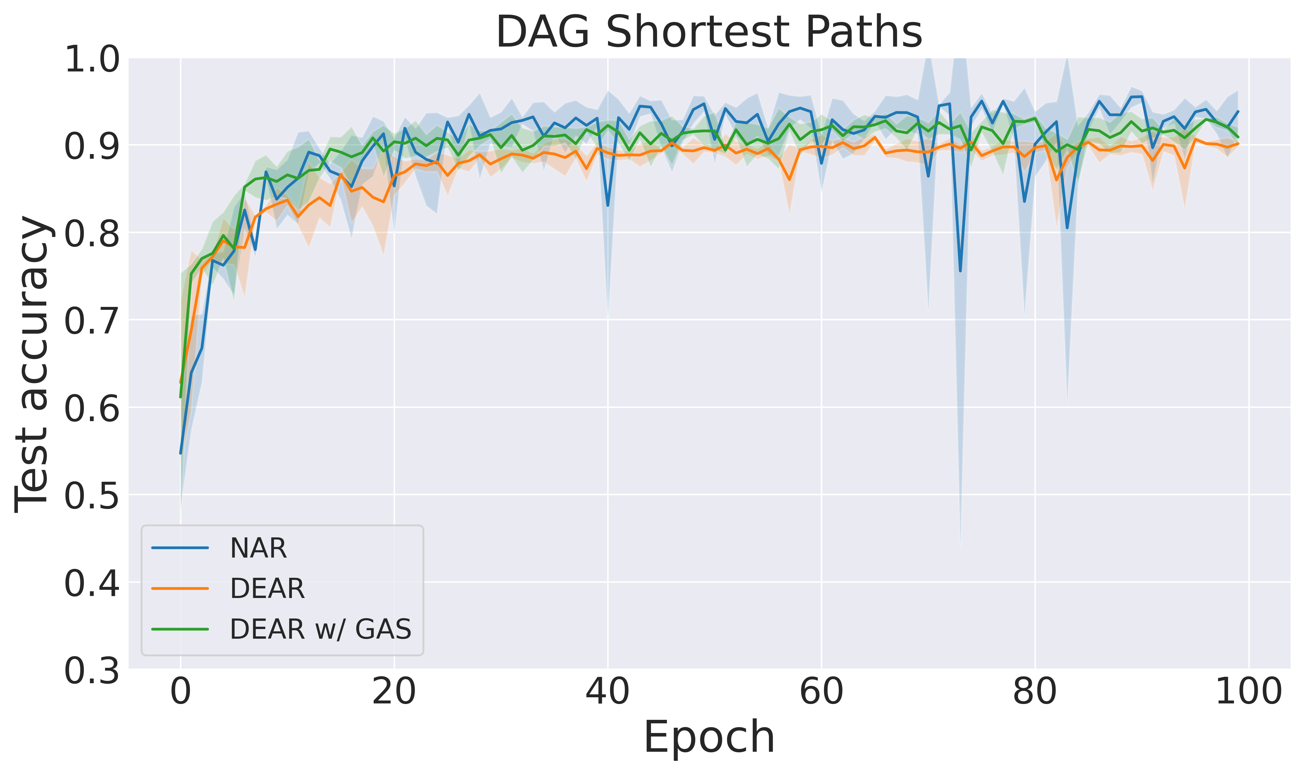
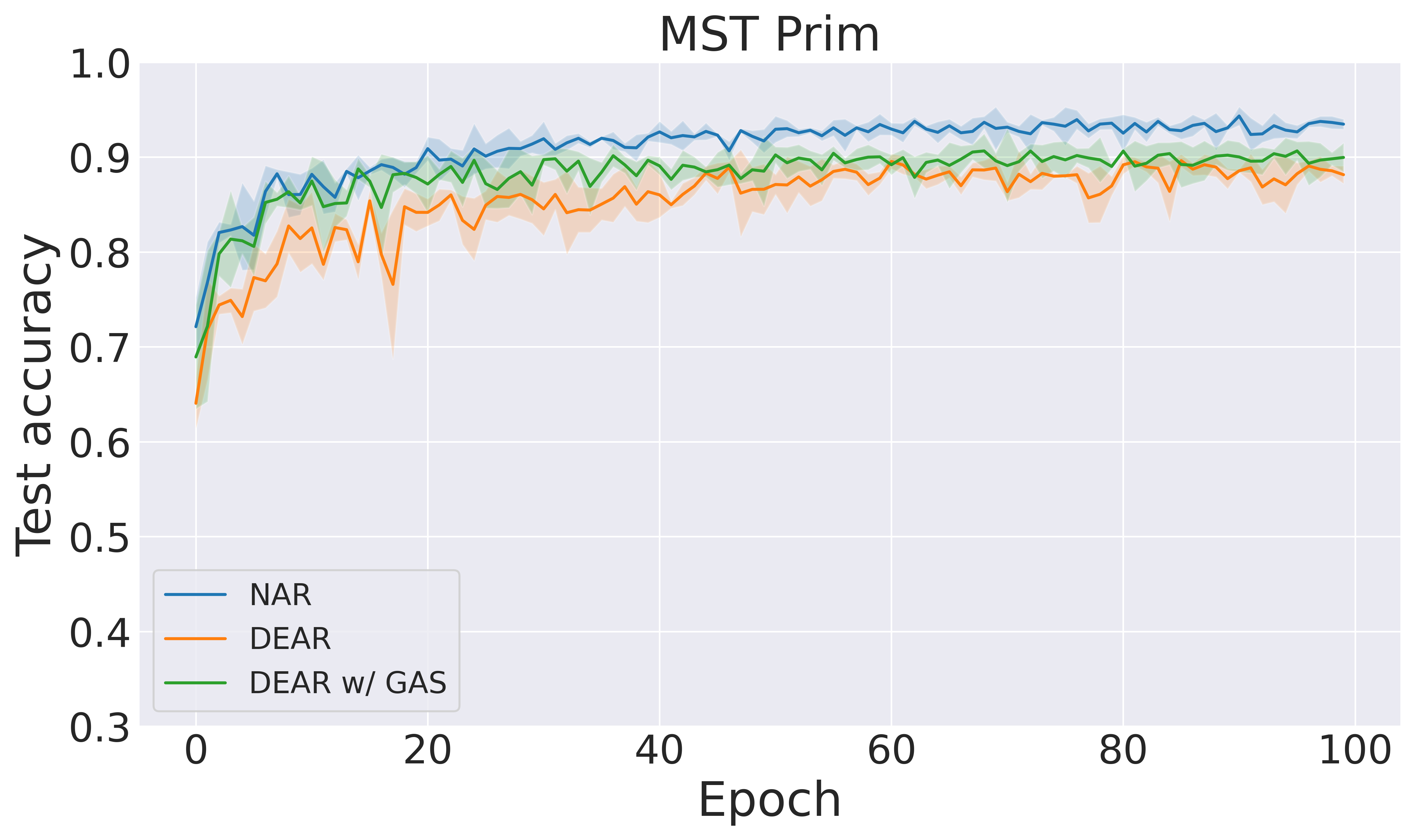
Figure 5: Alignment (DEAR w/ GAS) leads to improvements OOD

Table 2: Test accuracy with and without alignment.

	DSP	MST-Prim	Binary Search
NAR	$94.21\%\pm 1.77$	$93.56\%\pm 0.77$	$94.67\%\pm 2.31$
DEAR	$89.81\%\pm 0.14$	$88.67\%\pm 0.74$	$59.00\%\pm 12.3$
DEAR (alignment)	$89.65\%\pm 2.95$	$90.37\%\pm 1.19$	$77.33\%\pm 4.51$

Results are presented in Table 2. At first glance, the only algorithm that substantially improved was binary search, giving an almost 20% increase. The final test accuracy, however, does not represent all reality: Figure 4 shows that the task train loss (loss excluding any regularisers) for the model with alignment decreases, compared to no alignment and reaches similar levels as the one observed for the non-DEQ solution. So, is it overfitting again? We argue it is not. Figure 5 shows that the test (OOD) accuracy per epoch increases when using alignment, reaching similar accuracies to NAR for the DAG shortest path problem and improving over plain DEAR for MST-Prim, suggesting that choosing the right model using validation seed is hard in NAR [34]. Lastly, we would like to note that: 1) although granola+stochasticity does bring benefits on its own, alignment is necessary to narrow the gap to the NAR training loss (Appendix J); 2) We never reached perfect (0) alignment loss, suggesting better alignment techniques may further boost performance.

Table 3: Mean inference time in seconds per sample. Measured on an RTX 4090 GPU. Up/down arrows denote improvements/deteriorations. ${\color[rgb]{0,0.4453125,0.8125}\approx}$ is used when difference is negligible. A double symbol is used for substantial ($5\times$) differences.

	Bellman-F. ${\color[rgb]{0.83984375,0.03125,0.23046875}\uparrow}$	Floyd-W. ${\color[rgb]{0.83984375,0.03125,0.23046875}\uparrow}$	DSP ${\color[rgb]{0.33203125,0.6484375,0.109375}\downarrow}$	MST Prim ${\color[rgb]{0.33203125,0.6484375,0.109375}\downarrow}$	BFS ${\color[rgb]{0.83984375,0.03125,0.23046875}\uparrow}$	DFS ${\color[rgb]{0.33203125,0.6484375,0.109375}\downarrow\downarrow}$	SCC ${\color[rgb]{0.33203125,0.6484375,0.109375}\downarrow\downarrow}$	Search (Binary) ${\color[rgb]{0,0.4453125,0.8125}\approx}$	Minimum ${\color[rgb]{0.33203125,0.6484375,0.109375}\downarrow}$	Sort (Insertion) ${\color[rgb]{0.33203125,0.6484375,0.109375}\downarrow\downarrow}$
NAR◆	0.0118	0.0916	0.1334	0.0708	0.0094	0.2440	0.4017	0.0125	0.0684	0.5680
DEAR	0.0215	0.1102	0.0345	0.0297	0.0137	0.0478	0.0253	0.0131	0.0174	0.0260

Table 4: DEAR is architecture invariant and can also run with a Triplet-MPNN processor.

	Floyd-W.	DFS	SCC	Search (Parallel)	Sort	Overall
NAR◆	$61.86\%\pm 1.57$	$31.20\%\pm 4.02$	$\mathbf{46.84\%\pm 1.70}$	$\mathbf{93.33\%\pm 0.58}$	$63.67\%\pm 39.97$	$59.18\%$
DEAR (ours)	$\mathbf{62.29\%\pm 2.71}$	$\mathbf{42.73\%\pm 2.79}$	$45.12\%\pm 1.52$	$87.00\%\pm 5.57$	$\mathbf{82.34\%\pm 9.46}$	$\mathbf{63.90\%}$

DEARs are highly parallel

DEAR is not bound to follow sequential trajectories and GNNs are more aligned to parallel algorithms than to sequential ones [16]. As the cost for one step of DEAR (GNN iteration + solver) is at least as high as one step of an NAR model (GNN iteration only), we used the inference speed of a DEAR as a measure of how parallel the final learnt algorithm is. Results are presented in Table 3. An immediate observation is that DEAR improves inference times across almost all algorithms. The only ones that were executed slower are: 1) Bellman-Ford and BFS, which are highly parallelised in the CLRS-30 implementation, so an improvement on them was unlikely; 2) Floyd-Warshall where the difference, although present, is marginal and we account it to the added overhead from the solver; 3) Binary search, where performance was almost identical. These results suggest that although not always guaranteed (the case for searching), it is very likely that a DEAR will learn a parallel algorithm. The most substantial improvements, in line with our past observations in Engelmayer et al., [16], were on the tasks of sorting and strongly-connected components.

DEARs are foundational

Up until this point, DEAR was run with a PGN processor, which is a lightweight, yet well-performant NAR processor architecture. The last set of experiments aims to show that equilibrium reasoning is not tied to only one type of processor/architecture. It is rather a class of models/foundational model as it can natively support different types of processors. To verify this claim, we present results with DEAR using the Triplet-MPNN architecture in Table 4. As Triplet-MPNN is computationally expensive, we tested algorithms for which NAR with Triplet-MPNN improves over NAR with PGN. Results indeed confirm that we are not limited to a single type of processor with DEAR, and, as expected, the best overall performance is achieved when using DEAR with the more expressive, Triplet-MPNN, processor.

6 Conclusion

Our investigations with equilibrium models have shown that it is possible and even beneficial to merge NAR and DEQs. While our models attained very competitive performance, there are certain limitations that need to be addressed: 1) Better algorithms for alignment can help close the gap even further for Prim’s algorithm and binary search; 2) Better model selection is needed in order to know which DEARs would perform well OOD; 3) Graph rewiring techniques may be needed to prevent overfitting with CGP; 4) Algorithmic-aligned criteria for fixed-point may boost OOD generalisation for sequential algorithms. The last point is motivated by the fact that for each step, these algorithms update only a few nodes in the graph, keeping the rest untouched.

Appendix A IMP: Definitions and examples

Anything highlighted in blue below, is part of the IMP language. Subexpressions, to avoid confusion, are not coloured.

IMP consists of:

• numbers – 1, -20, 13930

• locations – AVariableName, AnotherVar, ArrayName$[$11$]$

• arithmetic expressions – (5+4)*3, but also A*55. Note how variables can be parts of arithmetic expressions.

• boolean expressions – true, false, but also X==0, 3*A<B and X==0 $\land$ 3*A<B. Note how boolean expressions can be made by using variables or using boolean logic on sub-expressions.

• commands – Commands can be one of:

  • skip, which is a no-op

  • X:=a, where X is assigned the value of arithmetic expression $a$. An example $a$ is 3*B+C

  • if $b$ then $c_{0}$ else $c_{1}$ where $b$ is a boolean expression and $c_{0}$, $c_{1}$ are commands. For example if A < B then C:=0 else C:=A-B which sets C to the difference of A and B, if it is positive

  • ($c_{0}$;$c_{1}$)

  • $\texttt{{\color[rgb]{0.0600000000000001,0.46,1}while}}\ b\ \texttt{{\color[rgb]{0.0600000000000001,0.46,1}do}}\ c$ which is a while loop repeating command $c$ as long as boolean expression $b$. A (classic) example is (Y:=1; while X > 0 do (Y:=X*Y; X:=X-1)), which finds the factorial of X and saves it in Y.

Appendix B Fixed point of a while loop – example

Below, we will denote the state as $[A\mapsto a,B\mapsto b,\dots]$. It means that the value of variable $A$ is $a$ and so on.

Consider the facorial example from above removing the explicit set of Y to 1. To find the denotation $\llbracket w\rrbracket=\llbracket$while X > 0 do (Y:=X*Y; X:=X-1)$\rrbracket$, we first define our $f_{b,c}$

$$f_{b,c}(w)([X\mapsto x,Y\mapsto y])=\begin{cases}{w}\left([X\mapsto x-1,Y\mapsto y*x]\right)&\text{if }X>0\\ [X\mapsto x,Y\mapsto y]&\text{otherwise}\end{cases}$$

The equivalent definition if we were to keep the lambdas from the original text is

$$f_{b,c}=\lambda w\in(State\rightharpoonup State).\lambda s\in State.\ \begin{cases}{w}\left([X\mapsto x-1,Y\mapsto y*x]\right)&\text{if }X>0\\ [X\mapsto x,Y\mapsto y]&\text{otherwise}\end{cases}$$

but we will work with the first definition as it is more compact.

The approximations of $f^{n}_{b,c}$ starting from $f^{0}_{b,c}=\bot$ are:

$$f^{1}_{b,c} =f_{b,c}(f^{0}_{b,c})([X\mapsto x,Y\mapsto y]) =$$

$$=f_{b,c}(\bot)([X\mapsto x,Y\mapsto y]) = \begin{cases}{\bot}\left([X\mapsto x-1,Y\mapsto y*x]\right)&\text{if }x>0\\ [X\mapsto x,Y\mapsto y]&\text{otherwise}\end{cases}$$

$$= \begin{cases}\text{undefined}&\text{if }x>0\\ [X\mapsto x,Y\mapsto y]&\text{otherwise}\end{cases}$$

$$f^{2}_{b,c} =f_{b,c}(f^{1}_{b,c})([X\mapsto x,Y\mapsto y]) = \begin{cases}{f^{1}_{b,c}}\left([X\mapsto x-1,Y\mapsto y*x]\right)&\text{if }x>0\\ [X\mapsto x,Y\mapsto y]&\text{otherwise}\end{cases}$$

$$= \begin{cases}\text{undefined}&\text{if }x-1>0\\ [X\mapsto x-1,Y\mapsto y\ast x]&\text{if }x-1=0\\ [X\mapsto x,Y\mapsto y]&\text{if }x\leq 0\end{cases}$$

$$= \begin{cases}\text{undefined}&\text{if }x>1\\ [X\mapsto 0,Y\mapsto y]&\text{if }x=1\\ [X\mapsto x,Y\mapsto y]&\text{if }x\leq 0\end{cases}$$

$$f^{3}_{b,c} =f_{b,c}(f^{2}_{b,c})([X\mapsto x,Y\mapsto y]) = \begin{cases}{f^{2}_{b,c}}\left([X\mapsto x-1,Y\mapsto y*x]\right)&\text{if }x>0\\ [X\mapsto x,Y\mapsto y]&\text{if }x\leq 0\end{cases}$$

$$= \begin{cases}\text{undefined}&\text{if }x-1>1\\ [X\mapsto 0,Y\mapsto y\ast x]&\text{if }x-1=1\\ [X\mapsto x-1,Y\mapsto y]&\text{if }x-1\leq 0\\ [X\mapsto x,Y\mapsto y]&\text{if }x\leq 0\\ \end{cases}$$

$$= \begin{cases}\text{undefined}&\text{if }x>2\\ [X\mapsto 0,Y\mapsto y\ast 2]&\text{if }x=2\\ [X\mapsto 0,Y\mapsto y]&\text{if }x=1\\ [X\mapsto x,Y\mapsto y]&\text{if }x\leq 0\\ \end{cases}$$

$$\vdots$$

which for $n$ is:

$$f^{n}_{b,c} =\begin{cases}\text{undefined}&\text{if }x\geq n\\ [X\mapsto 0,Y\mapsto y\ast(x!)]&\text{if }0<x<n\\ [X\mapsto x,Y\mapsto y]&\text{if }x\leq 0\\ \end{cases}$$

The sequence obeys $f^{0}_{b,c}\sqsubseteq f^{1}_{b,c}\sqsubseteq f^{2}_{b,c}\sqsubseteq\dots\sqsubseteq f^{n}_{b,c}\sqsubseteq\dots$ (we can see that whenever $f^{n-1}_{b,c}$ is defined it agrees with $f^{n}_{b,c}$) and $f_{b,c}$ is monotonic ($f^{k}_{b,c}\sqsubseteq f^{l}_{b,c}\implies f_{b,c}(f^{k}_{b,c})\sqsubseteq f_{b,c}(f^{l}_{b,c})$).

For a given $X=x$, $f^{x+1}_{b,c}=f^{x+2}_{b,c}=\dots$ . The fixed point is the lub of the whole sequence is therefore:

$$f^{\infty}_{b,c}=\bigsqcup_{n\geq 0}f^{n}_{b,c}(\bot)=\begin{cases}[X\mapsto 0,Y\mapsto y\ast(x!)]&\text{if }x>0\\ [X\mapsto x,Y\mapsto y]&\text{if }x\leq 0\end{cases}$$

By a similar analysis, it is not hard show that the denotation of $\llbracket\texttt{{\color[rgb]{0.0600000000000001,0.46,1}while true do skip}}\rrbracket$ will be undefined.

Appendix C Can algorithms, as implemented in CLRS-30, have an equilibrium?

In this appendix, we have copied over some algorithms implementations from CLRS-30. Additionally, we have annotated how and when they follow the $\texttt{{\color[rgb]{0.0600000000000001,0.46,1}while}}\ b\ \texttt{{\color[rgb]{0.0600000000000001,0.46,1}do}}\ c$ construct. Algorithms, that are not necessarily solved via this construct (e.g. strongly connected components) were also included, so as to showcase if this would break.

⬇

1def bfs(A: _Array, s: int) -> _Out:

2 chex.assert_rank(A, 2)

3 probes = probing.initialize(specs.SPECS[’bfs’])

4 A_pos = np.arange(A.shape[0])

5 probing.push(

6 probes,

7 specs.Stage.INPUT,

8 next_probe={

9 ’pos’: np.copy(A_pos) * 1.0 / A.shape[0],

10 ’s’: probing.mask_one(s, A.shape[0]),

11 ’A’: np.copy(A),

12 ’adj’: probing.graph(np.copy(A))

13 })

14 reach = np.zeros(A.shape[0])

15 pi = np.arange(A.shape[0])

16 reach[s] = 1

17 # Initialisation code ends here

18

19 # implemented as do-while, but do-whiles are essentially

20 # c; while b do c

21 while True:

22

23 prev_reach = np.copy(reach)

24 probing.push(

25 probes,

26 specs.Stage.HINT,

27 next_probe={

28 ’reach_h’: np.copy(prev_reach),

29 ’pi_h’: np.copy(pi)

30 })

31 # command c: update reachability.

32 for i in range(A.shape[0]):

33 for j in range(A.shape[0]):

34 if A[i, j] > 0 and prev_reach[i] == 1:

35 if pi[j] == j and j != s:

36 pi[j] = i

37 reach[j] = 1

38

39 if np.all(reach == prev_reach): # boolean condition b: has reachability vector changed

40 break

41

42 probing.push(probes, specs.Stage.OUTPUT, next_probe={’pi’: np.copy(pi)})

43 probing.finalize(probes)

44 return pi, probes

Listing 1: BFS algorithm. Clearly implemented as $\texttt{{\color[rgb]{0.0600000000000001,0.46,1}while}}\ b\ \texttt{{\color[rgb]{0.0600000000000001,0.46,1}do}}\ c$.

⬇

1# The sampler

2class FloydWarshallSampler(Sampler):

3 """Sampler for all-pairs shortest paths."""

4

5 def _sample_data(

6 self,

7 length: int,

8 p: Tuple[float, ...] = (0.5,),

9 low: float = 0., # never changed in the data generation

10 high: float = 1., # never changed in the data generation

11 ):

12 graph = self._random_er_graph( # samples random ER graph with weights in [low;high)

13 nb_nodes=length,

14 p=self._rng.choice(p),

15 directed=False,

16 acyclic=False,

17 weighted=True,

18 low=low,

19 high=high)

20 return [graph]

21

22# The implementation

23def floyd_warshall(A: _Array) -> _Out:

24 """Floyd-Warshall’s all-pairs shortest paths (Floyd, 1962)."""

25

26 chex.assert_rank(A, 2)

27 probes = probing.initialize(specs.SPECS[’floyd_warshall’])

28

29 A_pos = np.arange(A.shape[0])

30

31 probing.push(

32 probes,

33 specs.Stage.INPUT,

34 next_probe={

35 ’pos’: np.copy(A_pos) / A.shape[0],

36 ’A’: np.copy(A),

37 ’adj’: probing.graph(np.copy(A))

38 })

39

40 D = np.copy(A)

41 Pi = np.zeros((A.shape[0], A.shape[0]))

42 msk = probing.graph(np.copy(A))

43

44 for i in range(A.shape[0]):

45 for j in range(A.shape[0]):

46 Pi[i, j] = i

47

48 # Initialisation code ends here

49

50 # for loops are while loops

51 # ‘‘for k in range(N)’’ is equivalent to ‘‘k:=0; while (i<N) do (c; k:=k+1)’’

52 # NOTE #1 The NN, however, has to learn to increase the k, solely

53 # based on the ‘pos‘ input feature; having a ‘pred’ feature,

54 # (as in string algorithms) might have been more appropriate

55

56 # NOTE #2 *Since the sampler (above) only samples positive edge weights*

57 # no negative-weight cycles can exist. Hence any reruns of the inner two

58 # for loops, after k iteraitons have passed will not change matrix D.

59

60 # boolean condition b: k iterations have passed

61 # (a necessary, *but not sufficient* condition is that D remains unchanged)

62 for k in range(A.shape[0]):

63 prev_D = np.copy(D)

64 prev_msk = np.copy(msk)

65

66 probing.push(

67 probes,

68 specs.Stage.HINT,

69 next_probe={

70 ’Pi_h’: np.copy(Pi),

71 ’D’: np.copy(prev_D),

72 ’msk’: np.copy(prev_msk),

73 ’k’: probing.mask_one(k, A.shape[0])

74 })

75

76 # command c: update D for intermediate vertex k

77 for i in range(A.shape[0]):

78 for j in range(A.shape[0]):

79 if prev_msk[i, k] > 0 and prev_msk[k, j] > 0:

80 if msk[i, j] == 0 or prev_D[i, k] + prev_D[k, j] < D[i, j]:

81 D[i, j] = prev_D[i, k] + prev_D[k, j]

82 Pi[i, j] = Pi[k, j]

83 else:

84 D[i, j] = prev_D[i, j]

85 msk[i, j] = 1

86

87 probing.push(probes, specs.Stage.OUTPUT, next_probe={’Pi’: np.copy(Pi)})

88 probing.finalize(probes)

89

90 return Pi, probes

Listing 2: Floyd-Warshall algorithm and its sampler (above). Can also be viewed as $\texttt{{\color[rgb]{0.0600000000000001,0.46,1}while}}\ b\ \texttt{{\color[rgb]{0.0600000000000001,0.46,1}do}}\ c$, in CLRS-30.

⬇

1def strongly_connected_components(A: _Array) -> _Out:

2 """Kosaraju’s strongly-connected components (Aho et al., 1974)."""

3

4 chex.assert_rank(A, 2)

5 probes = probing.initialize(

6 specs.SPECS[’strongly_connected_components’])

7

8 A_pos = np.arange(A.shape[0])

9

10 probing.push(

11 probes,

12 specs.Stage.INPUT,

13 next_probe={

14 # < omitted for brevity >

15 })

16

17 scc_id = np.arange(A.shape[0])

18 color = np.zeros(A.shape[0], dtype=np.int32)

19 d = np.zeros(A.shape[0])

20 f = np.zeros(A.shape[0])

21 s_prev = np.arange(A.shape[0])

22 time = 0

23 A_t = np.transpose(A)

24

25 # Initialisation code ends here

26

27 # boolean condition b: there are unvisited (color[s]=0) vertices

28 for s in range(A.shape[0]):

29 if color[s] == 0:

30 s_last = s

31 u = s

32 v = s

33 probing.push(

34 probes,

35 specs.Stage.HINT,

36 next_probe={

37 # < omitted for brevity >

38 })

39 # command c: grey them (color=1) and recursively visit descendants

40

41 # NOTE command c is another while b’ do c’ with a stack

42 while True: # b’: stack is not empty

43 if color[u] == 0 or d[u] == 0.0:

44 time += 0.01

45 d[u] = time

46 color[u] = 1

47 probing.push(

48 probes,

49 specs.Stage.HINT,

50 next_probe={

51 # < omitted for brevity >

52 })

53 for v in range(A.shape[0]): # c’: add lowest id unvisited descendant of top-stack node to the top of the stack

54 if A[u, v] != 0:

55 if color[v] == 0:

56 color[v] = 1

57 s_prev[v] = s_last

58 s_last = v

59 probing.push(

60 probes,

61 specs.Stage.HINT,

62 next_probe={

63 # < omitted for brevity >

64 })

65 break

66

67 if s_last == u: # no descending

68 color[u] = 2

69 time += 0.01

70 f[u] = time

71

72 probing.push(

73 probes,

74 specs.Stage.HINT,

75 next_probe={

76 # < omitted for brevity >

77 })

78

79 if s_prev[u] == u: # and we are on top of the recursion

80 # although imaginary, in the implementation here,

81 # if a stack was used, it’d be empty in this if

82 # statement

83 assert s_prev[s_last] == s_last

84 break

85 pr = s_prev[s_last]

86 s_prev[s_last] = s_last

87 s_last = pr

88

89 u = s_last

90

91 color = np.zeros(A.shape[0], dtype=np.int32)

92 s_prev = np.arange(A.shape[0])

93

94 # boolean condition b’’: there are unvisited (color[s]=0) vertices

95 # (order of visiting depends on finishing time;

96 # see Introduction to algorithms, 4th edition, Chapter 20)

97 for s in np.argsort(-f):

98 if color[s] == 0:

99 s_last = s

100 u = s

101 v = s

102 probing.push(

103 probes,

104 specs.Stage.HINT,

105 next_probe={

106 # < omitted for brevity >

107 })

108 # NOTE command c is another while b’’’ do c’’’ with a stack

109 while True: # b’’’: stack is not empty

110 scc_id[u] = s

111 if color[u] == 0 or d[u] == 0.0:

112 time += 0.01

113 d[u] = time

114 color[u] = 1

115 probing.push(

116 probes,

117 specs.Stage.HINT,

118 next_probe={

119 # < omitted for brevity >

120 })

121 for v in range(A.shape[0]): # c’’’: add lowest id unvisited descendant of top-stack node to the top of the stack

122 if A_t[u, v] != 0:

123 if color[v] == 0:

124 color[v] = 1

125 s_prev[v] = s_last

126 s_last = v

127 probing.push(

128 probes,

129 specs.Stage.HINT,

130 next_probe={

131 # < omitted for brevity >

132 })

133 break

134

135 if s_last == u:

136 color[u] = 2

137 time += 0.01

138 f[u] = time

139

140 probing.push(

141 probes,

142 specs.Stage.HINT,

143 next_probe={

144 # < omitted for brevity >

145 })

146

147 if s_prev[u] == u: # same as before

148 assert s_prev[s_last] == s_last

149 break

150 pr = s_prev[s_last]

151 s_prev[s_last] = s_last

152 s_last = pr

153

154 u = s_last

155

156 probing.push(

157 probes,

158 specs.Stage.OUTPUT,

159 next_probe={’scc_id’: np.copy(scc_id)},

160 )

161 probing.finalize(probes)

162

163 return scc_id, probes

Listing 3: Kosaraju’s strongly connected components [40] algorithm. It is composed of four (two nested ones, sequenced one after the other) $\texttt{{\color[rgb]{0.0600000000000001,0.46,1}while}}\ b\ \texttt{{\color[rgb]{0.0600000000000001,0.46,1}do}}\ c$ constructs.

Appendix D Differences to Ibarz et al., [29]

Our differences are mostly required by software engineering rather than research, hence they live here. Differences are:

• Different DL framework (Pytorch [36])

• Ibarz et al., [29] use an extra nonlinearity after the GNN step. We found this to be not necessary (there are plenty of nonlinearities at the message function) for the baseline and to be making the training of DEARs less stable so we removed it.

• Sorting-based algorithms use a Sinkhorn operator to force the output to be a permutation. However, this gave very negative logits for the predictions at initialisation, leading to runs starting from a very high loss and converging to poorer minima. We fixed this by adding an off-centred leaky ReLU activation with the kink point at (-6, -6) right after the Sinkhorn operator. After conversion of logits to outputs via softmax, our change is mathematically equivalent to saying that the probability for each other node to be predecessor should not drop below $10^{-6}$.

Appendix E Picking least fixed point

For a given batch fixed point finding continues until all instances in the batch converge and at each step the solver is stepped on all instances. For a given instance, when two ${\mathbf{H}}^{(t)}$ and ${\mathbf{H}}^{(t^{\prime})}$ are under the threshold $\delta$, for some $t\leq t^{\prime}$, the torchdeq library prefers the state that has the lower distance to next state. Consequently, out the returned fixed points only one is guaranteed to be least – the one that require the most steps. This not only misaligns with domain theory, but also had the practical effect that the neural models require more iterations to converge the more we train them. Thus, we changed the library to choose the first ${\mathbf{H}}{(t)}$ that passes the fixed point criteriaq.

Appendix F Alignment algorithm

Assume we have computed pairwise distance matrices between the states and those are stored in a $T\times T_{\mathcal{G}}$ distance matrix ${\mathbf{D}}$ with elements $d_{i,j}$. Ignoring the required alignment of the last states, we focus on aligning the rest of the states. This is done via standard dynamic programming algorithm. The dynamic programming state we define is as follows: $dp_{i,j}$ is the most optimal alignment for the first $i$ DEAR states and first $j$ NAR states, with $dp_{0,j}=0$ (having leftover NAR states mean we skipped some, but we do not want to penalise that) and $dp_{i,0}=\infty$ (we want to align all DEAR states). We consider two recursive formulas, first one we use, the other we use when $T\leq T_{\mathcal{G}}$:

• when the $T>T_{\mathcal{G}}$, there are extra states. To avoid infinities we will allow for two DEAR states to align to a same state:

  $$dp_{i,j}=\min\begin{cases}dp_{i-1,j}+d_{i,j}&\text{aligning DEAR state $i$ and NAR state $j$, but allowing for}\\ &\text{previous states to align to it as well}\\ dp_{i,j-1}&\text{skipping alignment with state $j$}\end{cases}$$ (5)

• when the $T\leq T_{\mathcal{G}}$ we require that each DEAR state aligns to an unique NAR state:

  $$dp_{i,j}=\min\begin{cases}dp_{i-1,{\color[rgb]{0.55,0.14,1}j-1}}+d_{i,j}&\text{aligning DEAR state $i$ and NAR state $j$}\\ dp_{i,j-1}&\text{skipping alignment with state $j$}\end{cases}$$ (6)

  We have highlighted the difference to the above in purple.

The optimal alignment for the whole two sequence is stored in $dp_{T,T_{\mathcal{G}}}$. As both ${\mathbf{H}}^{(0)}$ and ${\mathbf{H}}^{(0)}_{\mathcal{G}}$ are concatenation of 0 vectors (due to how we initialise the latent state), their distance is always 0 and they will always align as required. To enforce alignment of the last state, we take the optimal value for the subsequences without last states $dp_{T-1,T_{\mathcal{G}}-1}$ and always (even when subsampling, see below) add the distances between the last states to the loss function.

As the above will always penalise longer DEQ trajectories, we divide $dp_{T-1,T_{\mathcal{G}}-1}$ by $T-1$ before including it in the loss function. Lastly, to allow for “intermediate” states (ones not necessarily matching a GNN state) to exist, we subsample randomly, without replacement, $T^{\prime}=\max(\lfloor\frac{T-1}{2}\rfloor,1)$ DEAR states and apply the dynamic programming algorithm with the subsampled sequence.

Appendix G Training loss: NAR vs DEAR

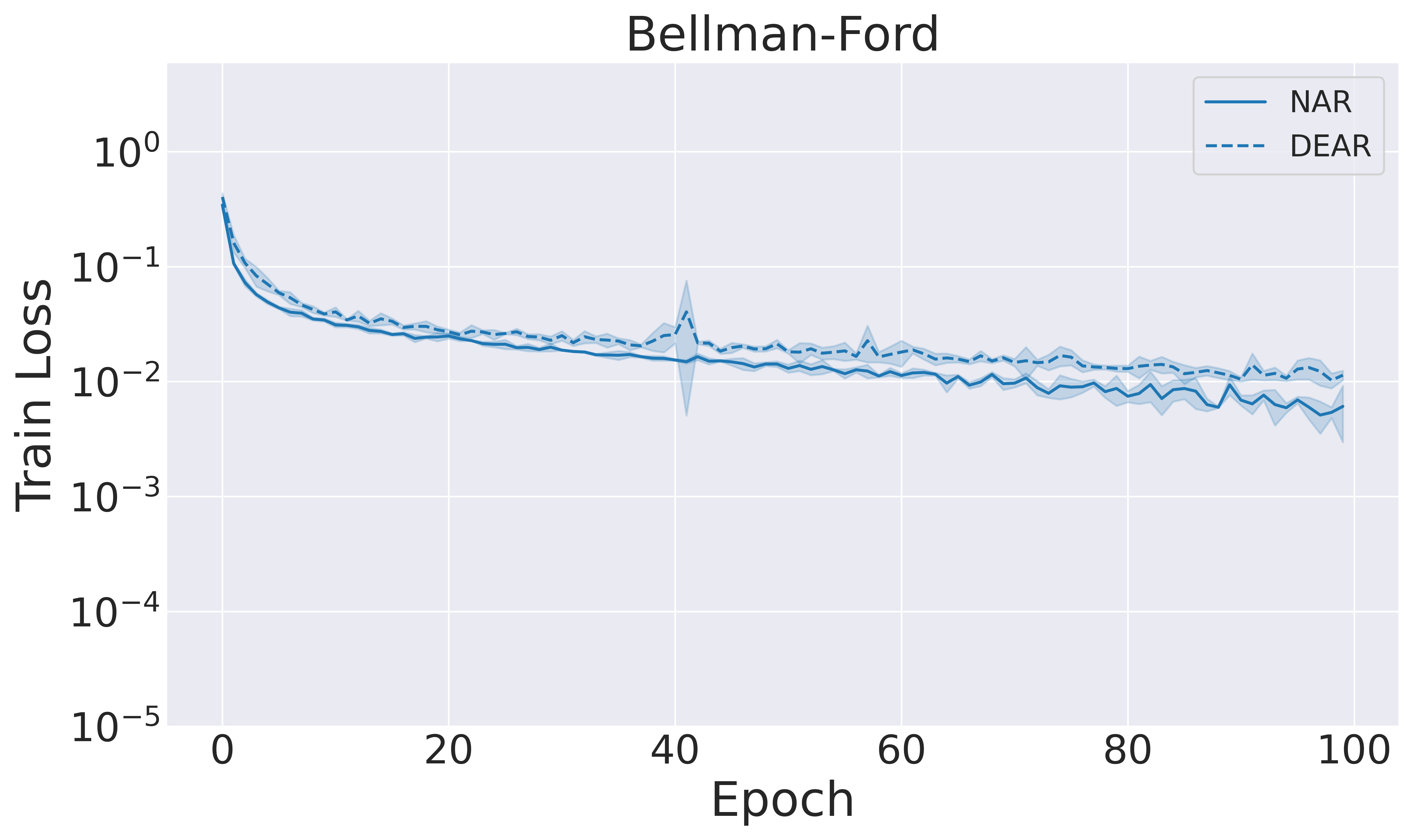
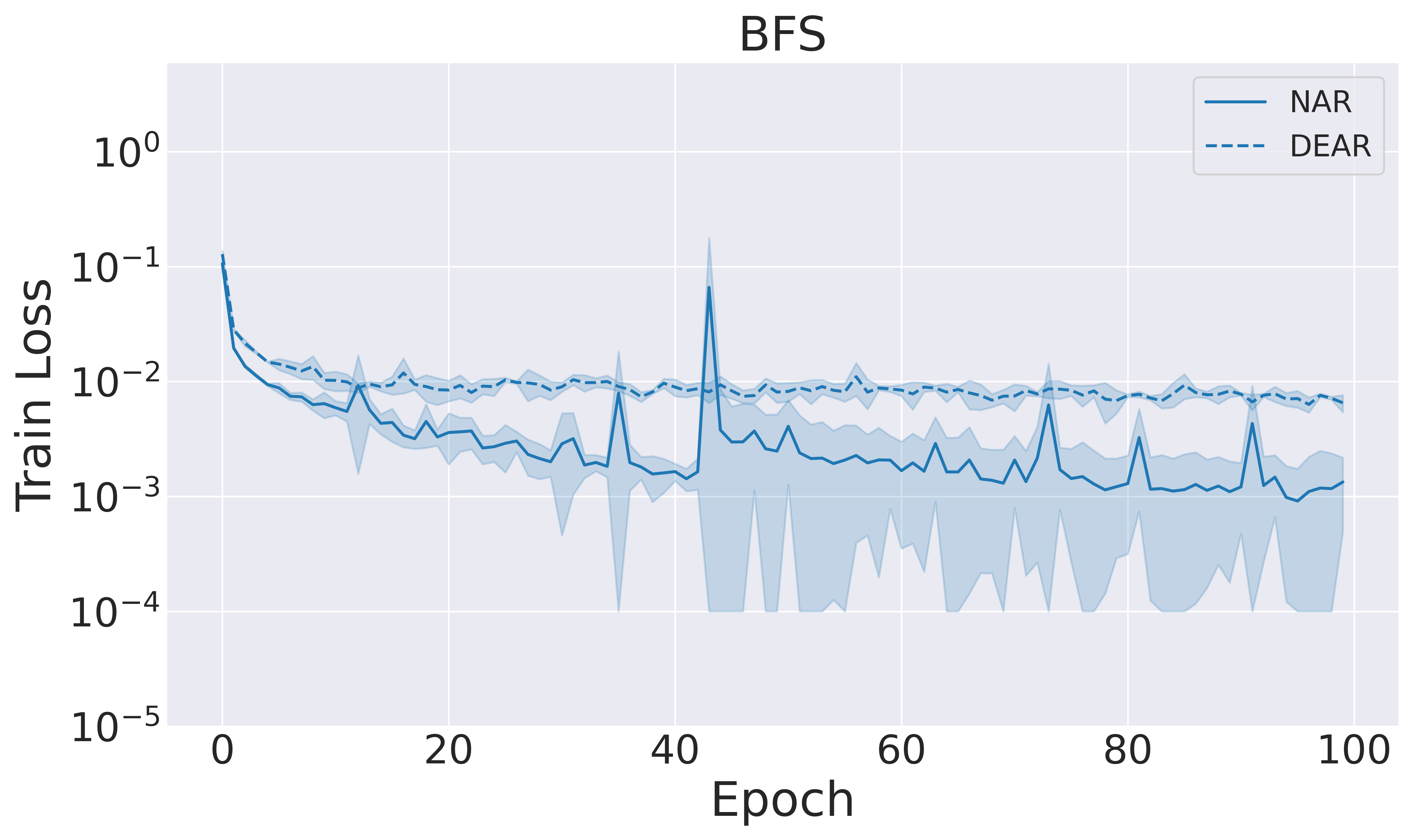
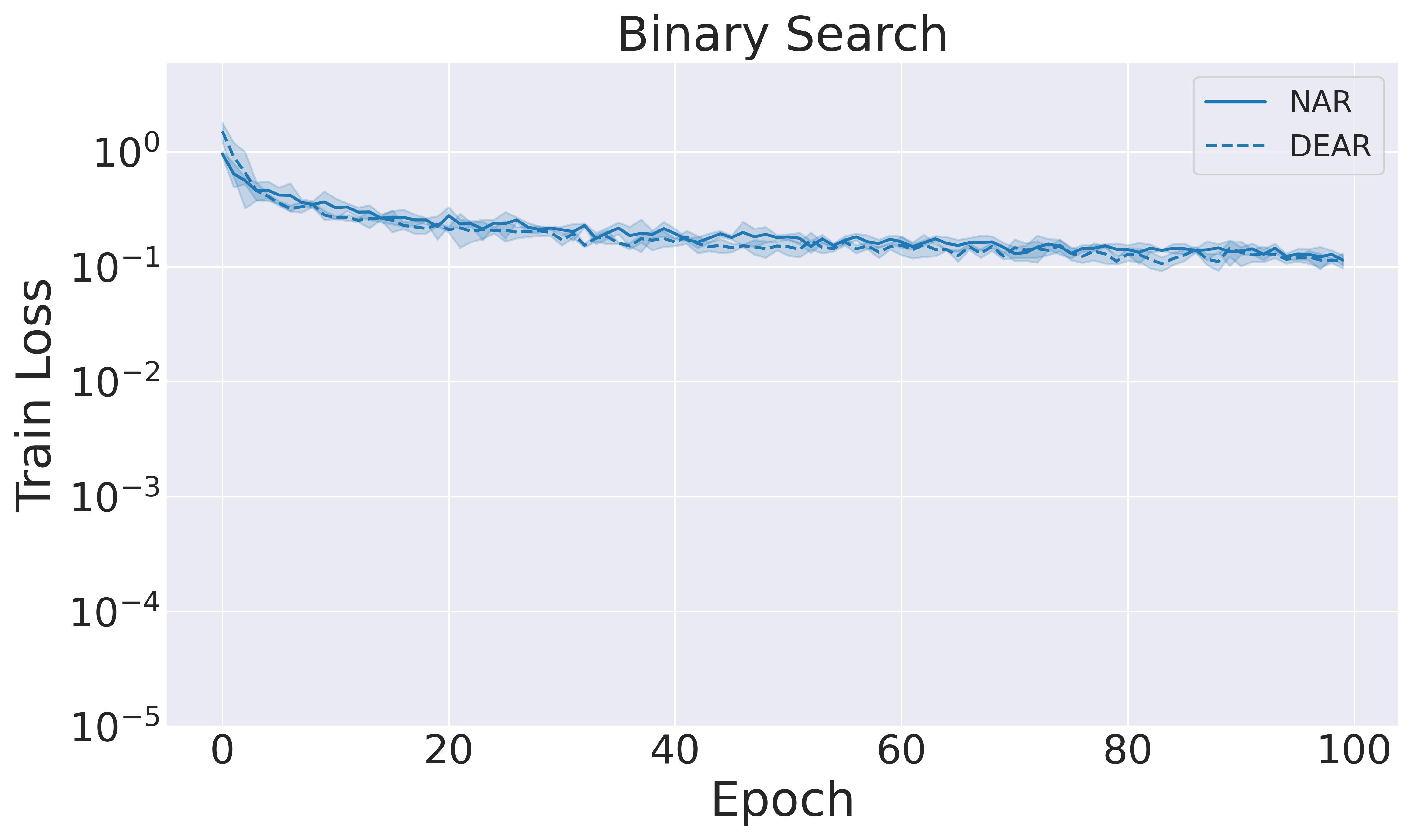
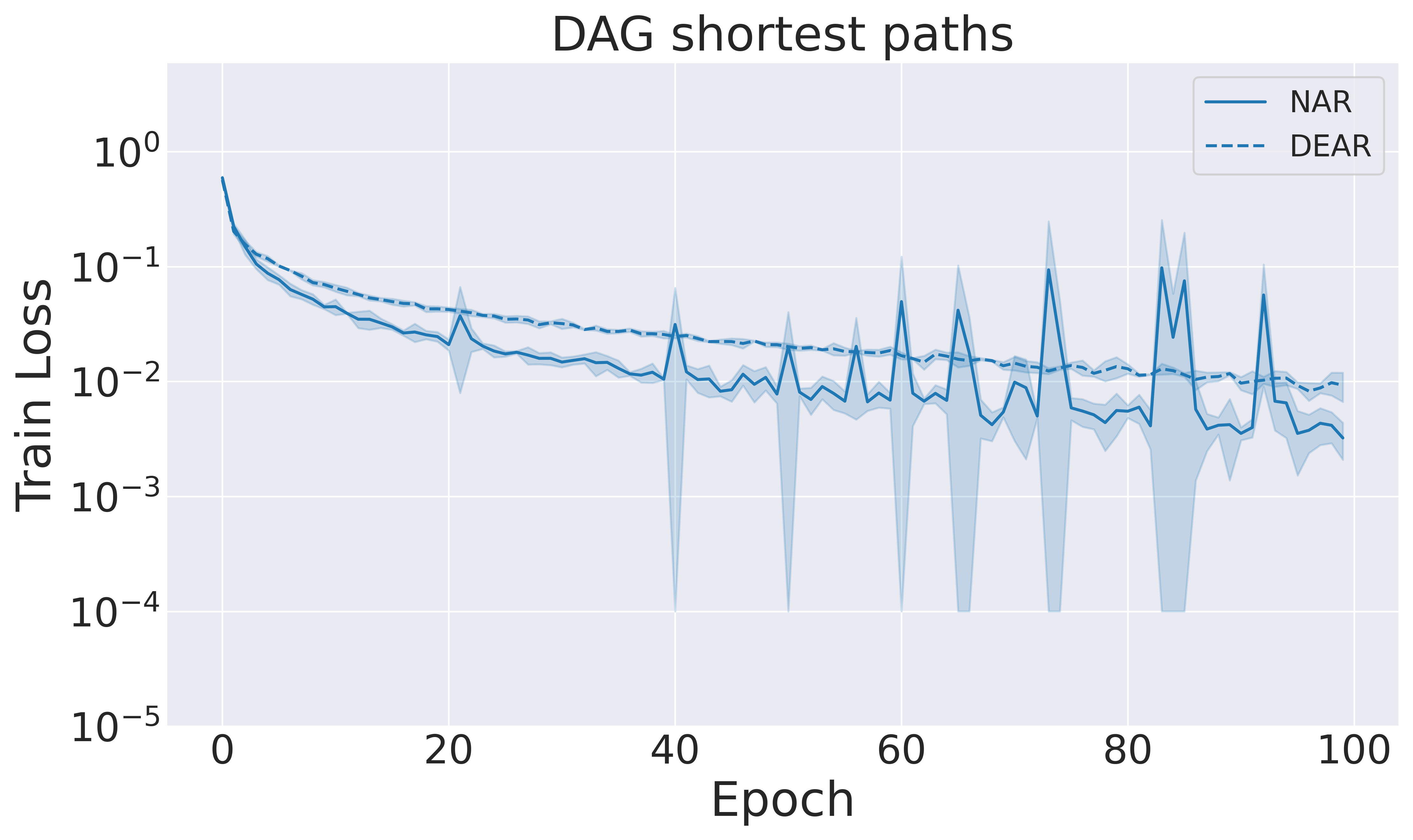
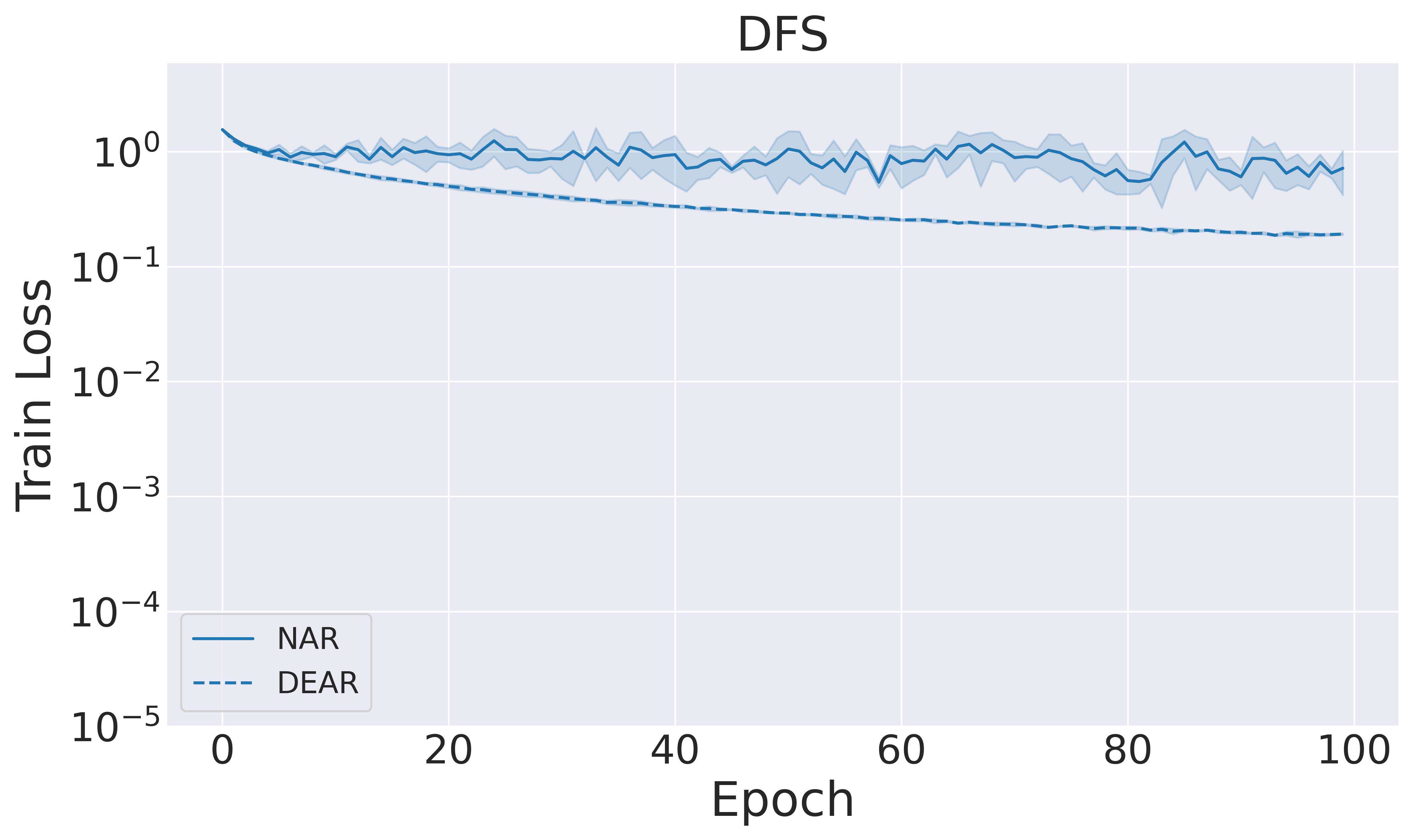
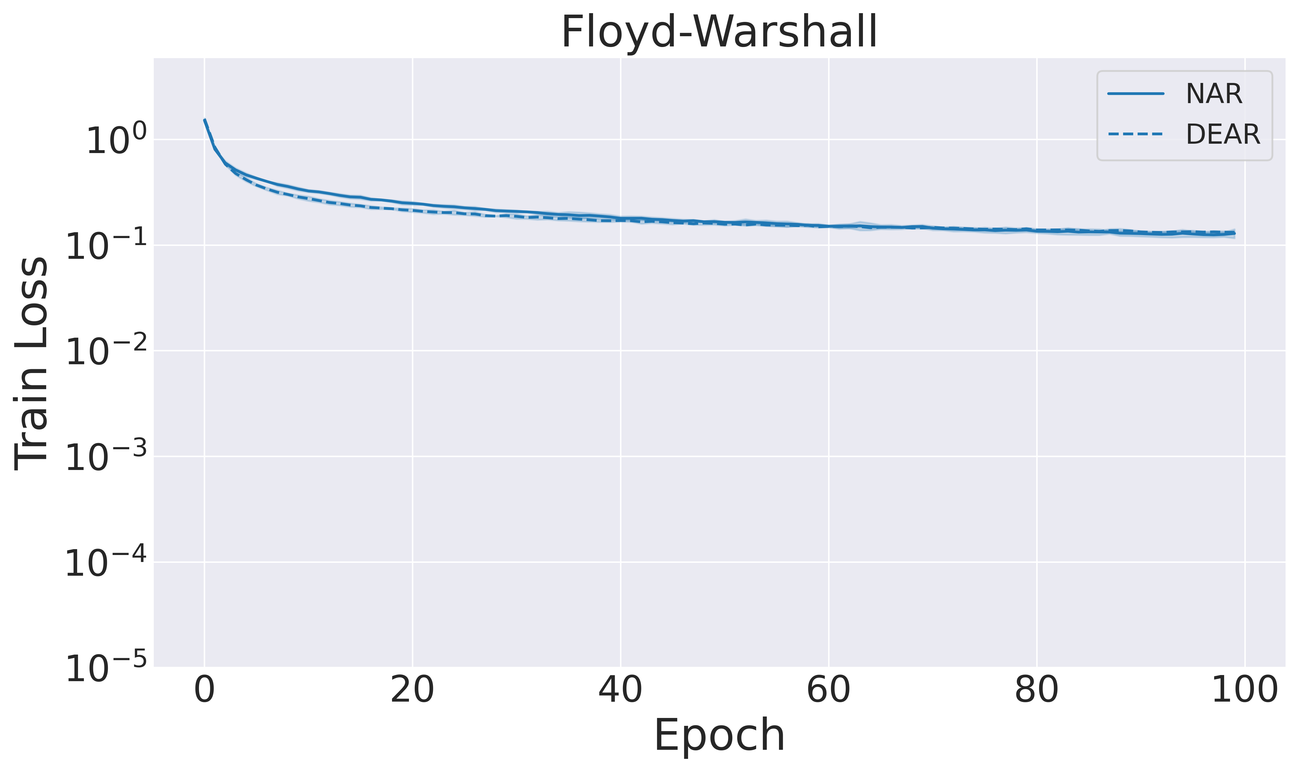
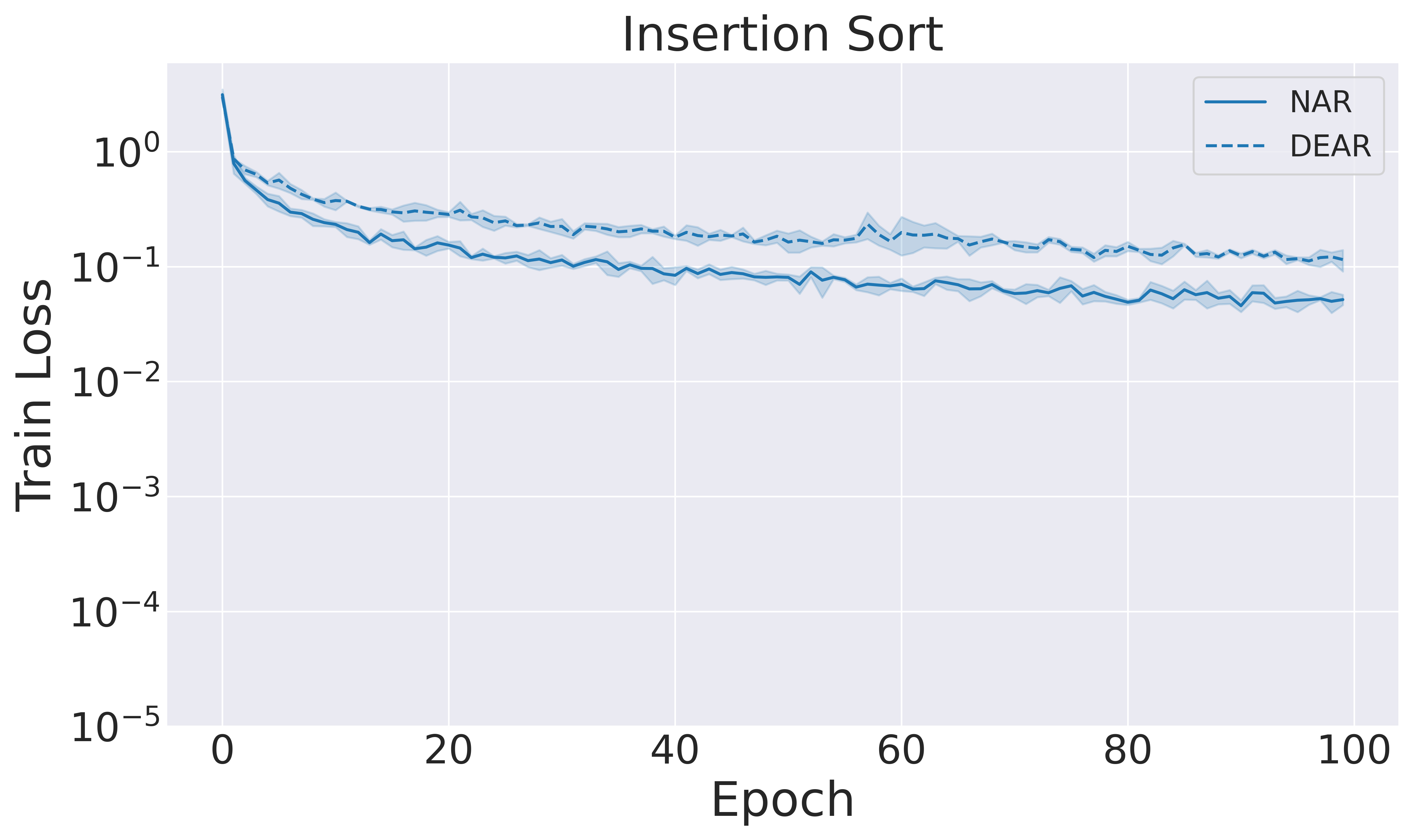
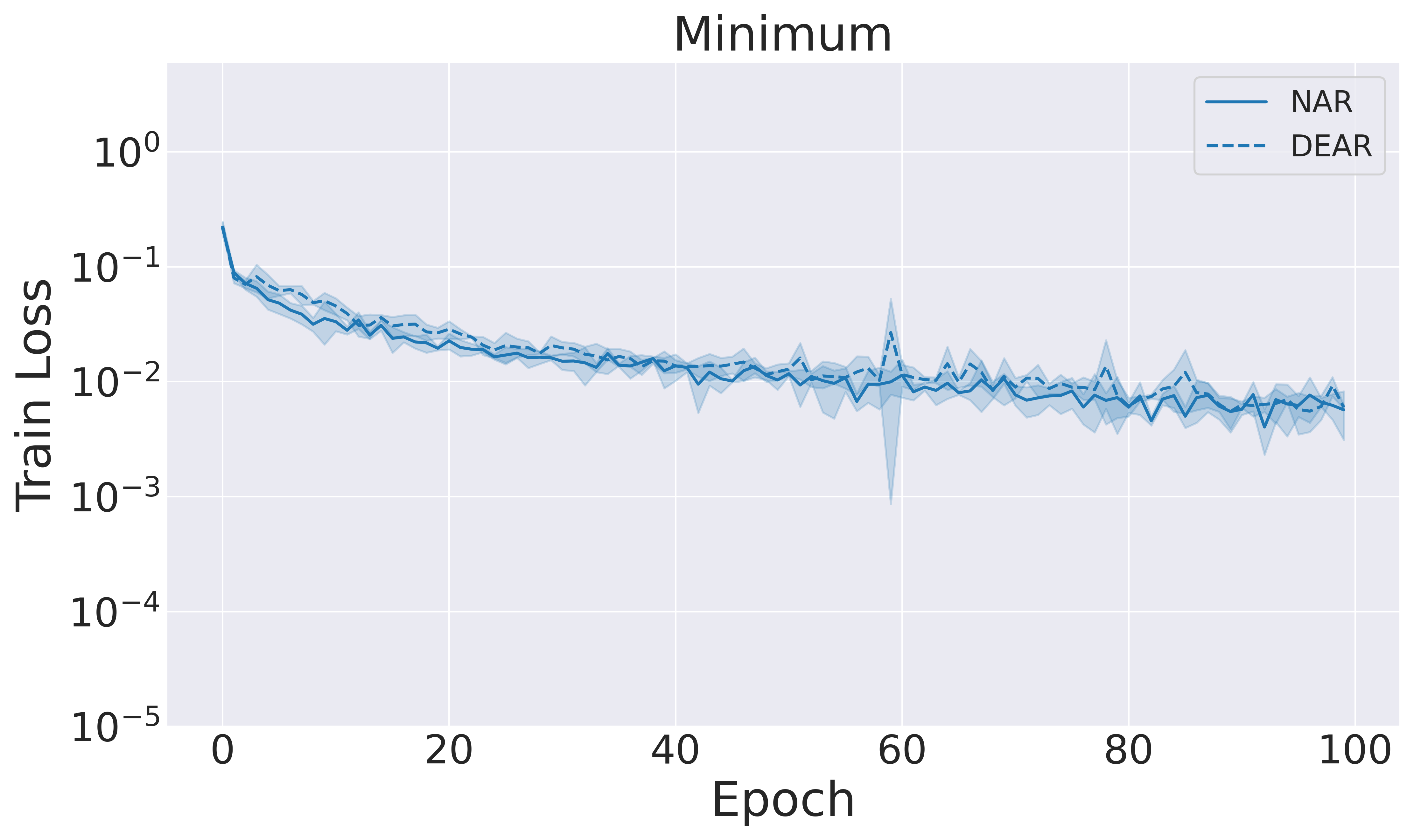
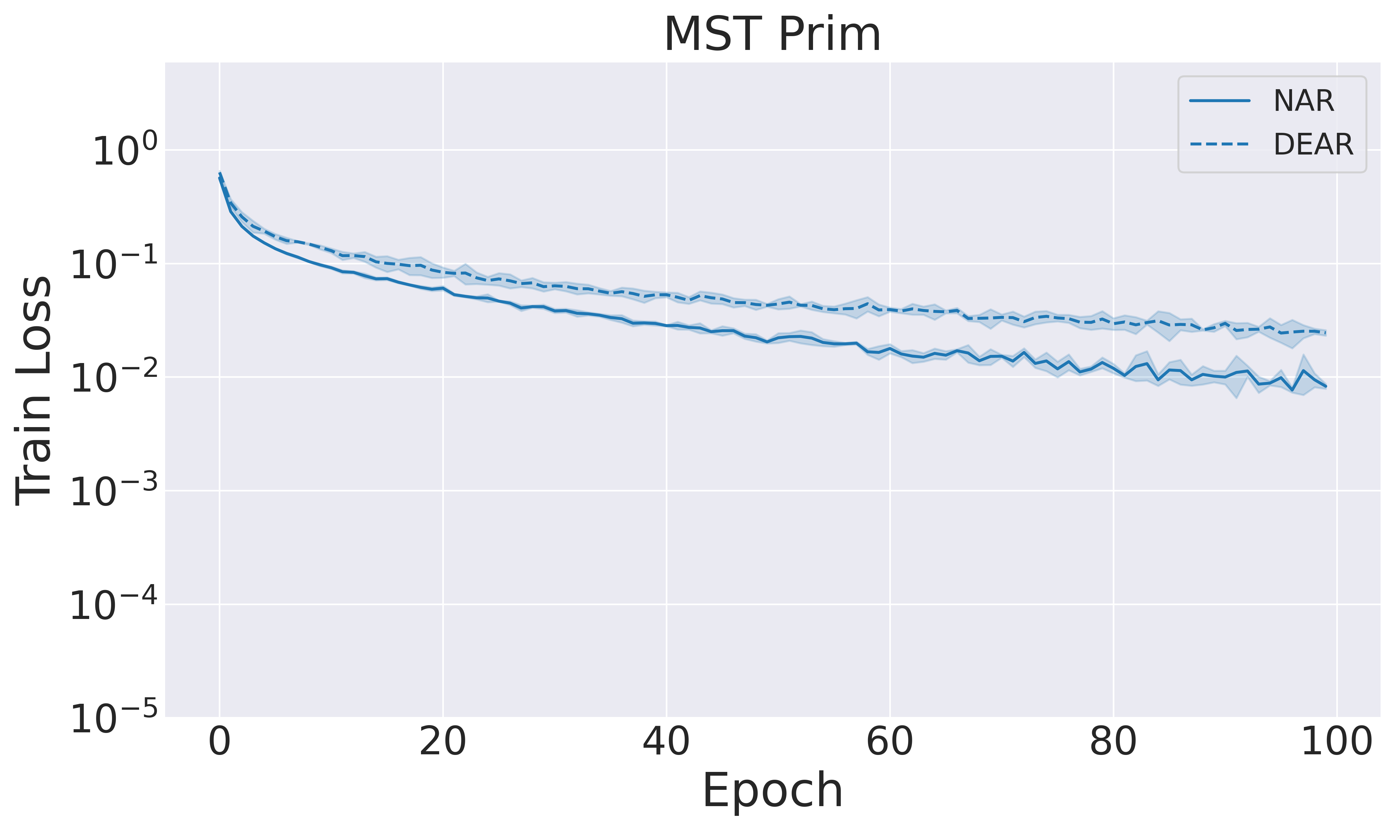
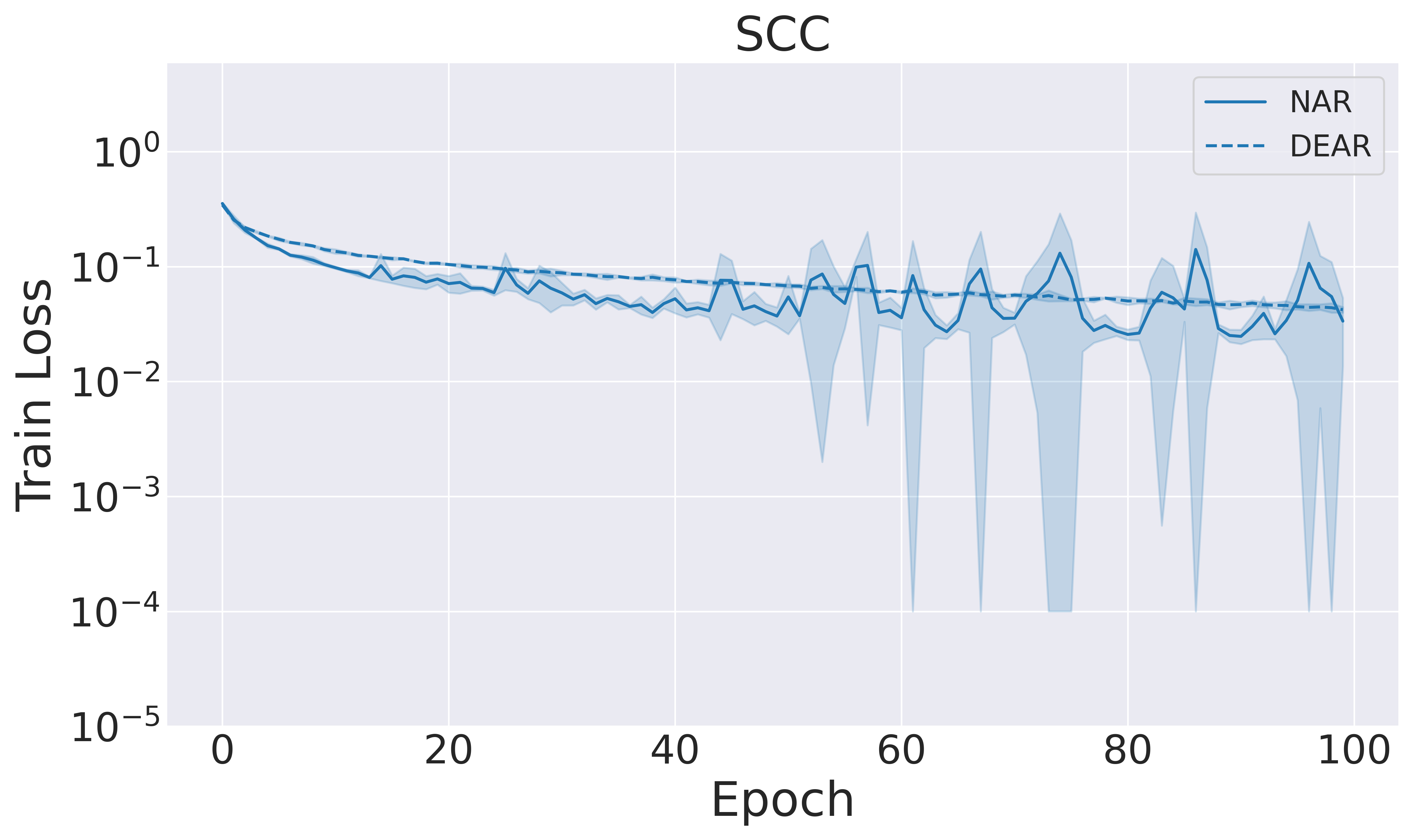
Figure 6: Side-by-side comparison of NAR vs DEAR. DEAR training loss is always within 1 order of magnitude of NAR. Note the log scale.

Appendix H Binary search anomalies

In the CLRS-30 implementation of binary search, we aim to find the place to insert the target value x in a sorted array A. Thus we need to point to the graph node that holds the smallest value in the array A, which is greater than x. However, if x>max (A), the answer is a pointer to the last value of the array, which by the convention used by CLRS-30 means we would be inserting x at the wrong place. In other words, the answer to A=[0.1, 0.2, 0.3] x=0.25 and A=[0.1, 0.2, 0.3] x=0.35 is the same – insert x to the left of 0.3. This contributed some noise, so we fixed the sampler to always give x within [0, max(A)). The other changes were to explicitly use graph & pointer instead of node & mask_one as the location & datatype of the pointer to the position in the array, also done by Engelmayer et al., [16]. Similarly to them, we also add an additional supervision signal, but at the output level rather than the hint level – teaching the models to predict which array elements are smaller than x (binary mask type).

Table 5: Fixing anomalies with CLRS-30’s binary search further increases our overall score making our approach very competitive to Triplet-MPNN. Notation taken from Table 1.

Algorithm	NAR◆	NAR◆ (Triplet-MPNN)	NAR♢ (LT)	DEAR (ours)
Search (Parallel)	$95.67\%\pm 0.58$	$93.33\%\pm 0.58$	$93.33\%\pm 3.05$	$85.67\%\pm 0.58$
New Overall	$71.52\%$	$77.58\%$	$70.97\%$	$78.38\%$

We reran the new, parallel version of search, reporting results in Table 5. Our model still falls short of the baselines, but the 26% increase in accuracy is large enough to give a slight overall advantage to DEAR over the Triplet-MPNN model. We do note, however, that the task of searching is mostly numerical (comparison between floating point numbers), resulting in DEAR overfitting a lot – recall that train accuracy was 95% even for the original (binary) search. We verified that if the training data is increased $3\times-5\times$, test accuracy becomes comparable to other models, regardless of which version is used.

Appendix I Training loss: DEAR vs DEAR w/ CGP

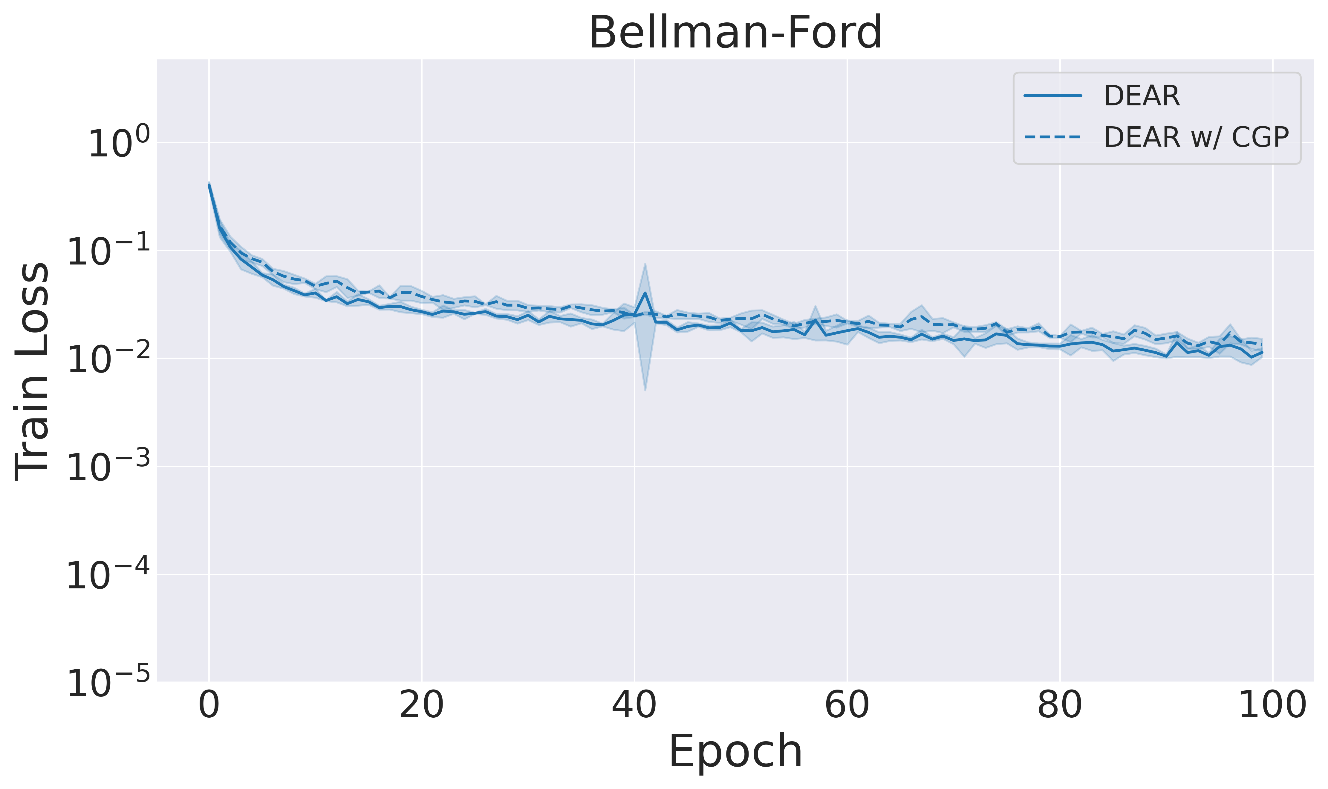
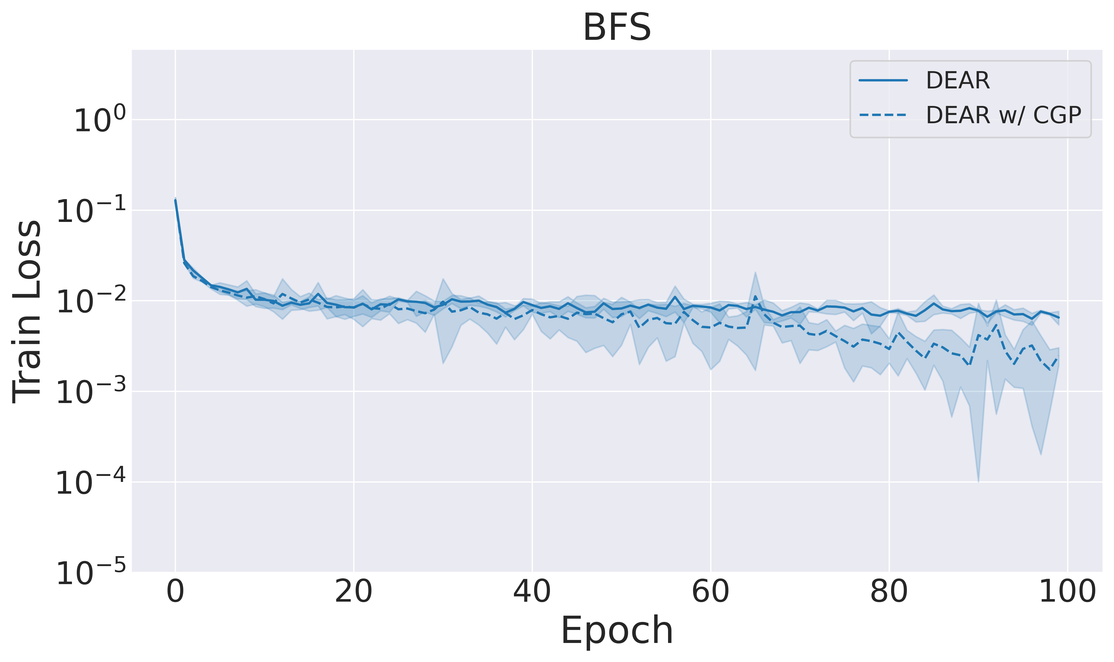
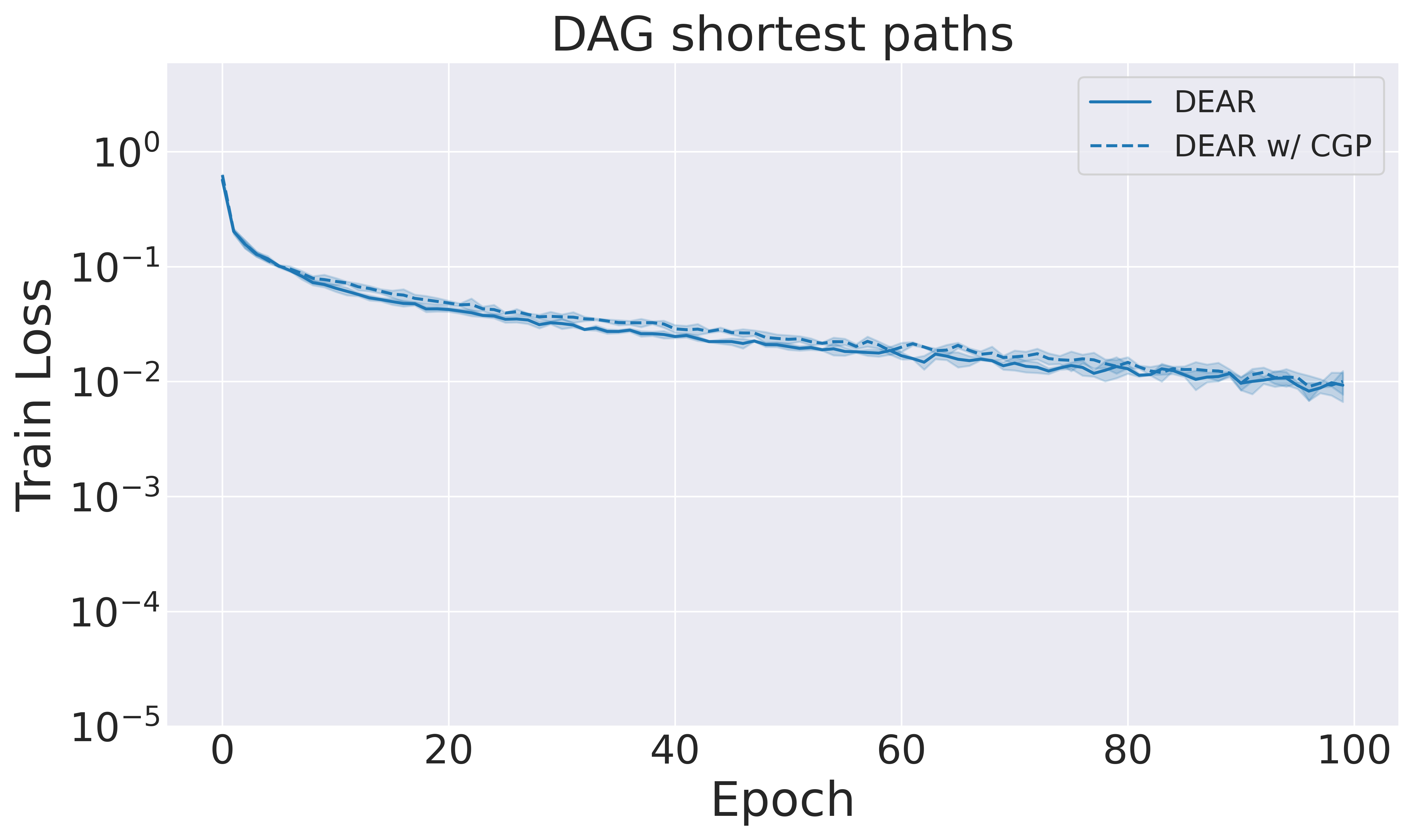
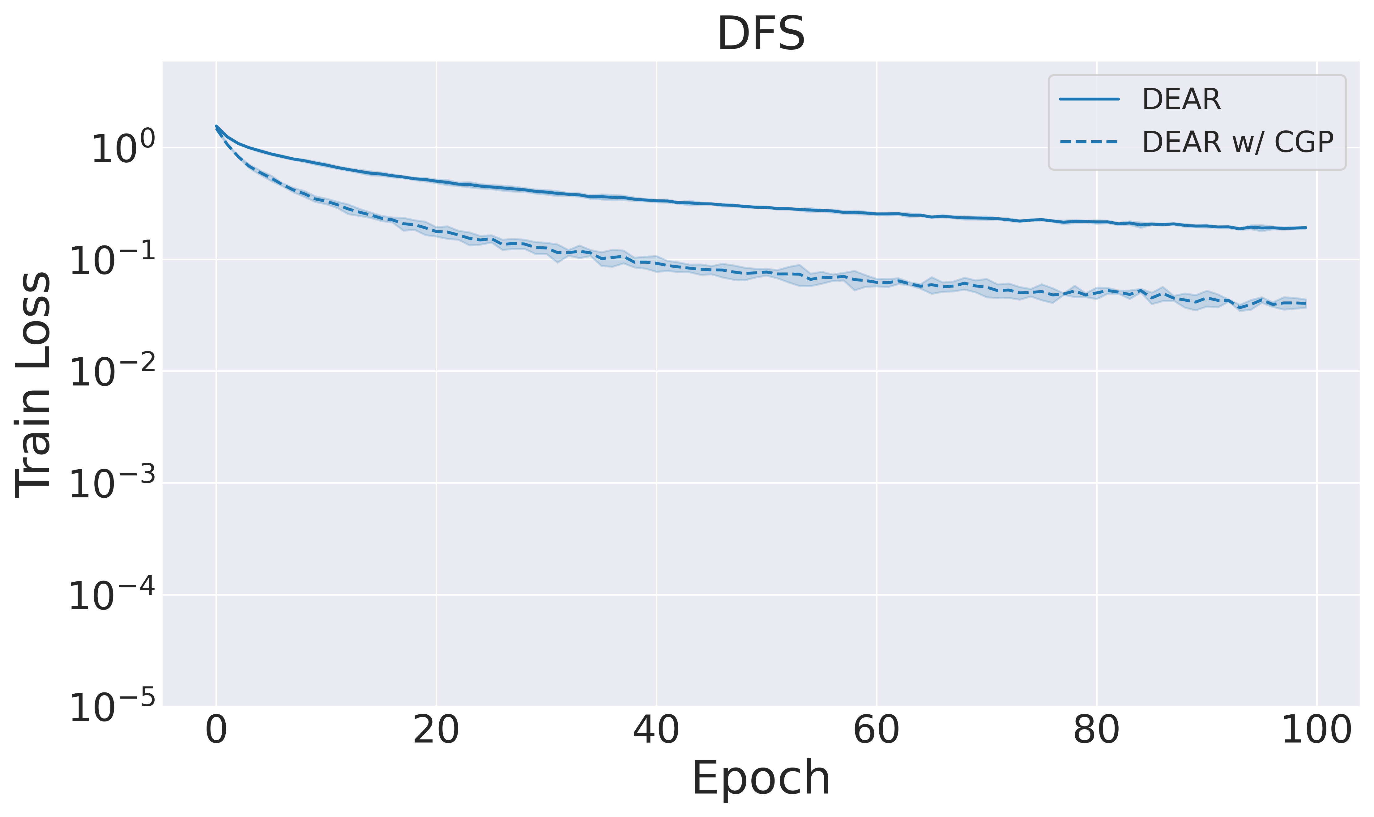
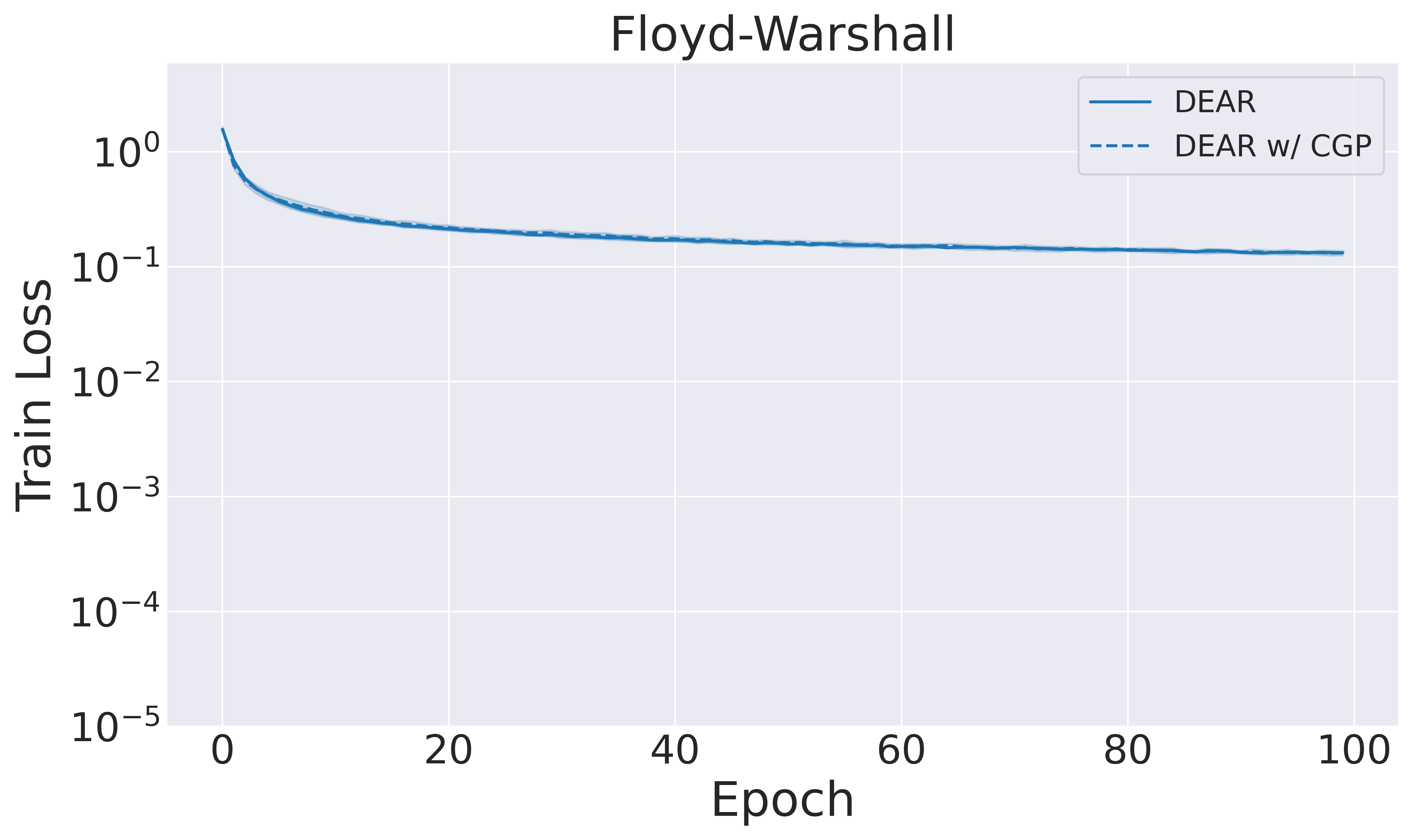
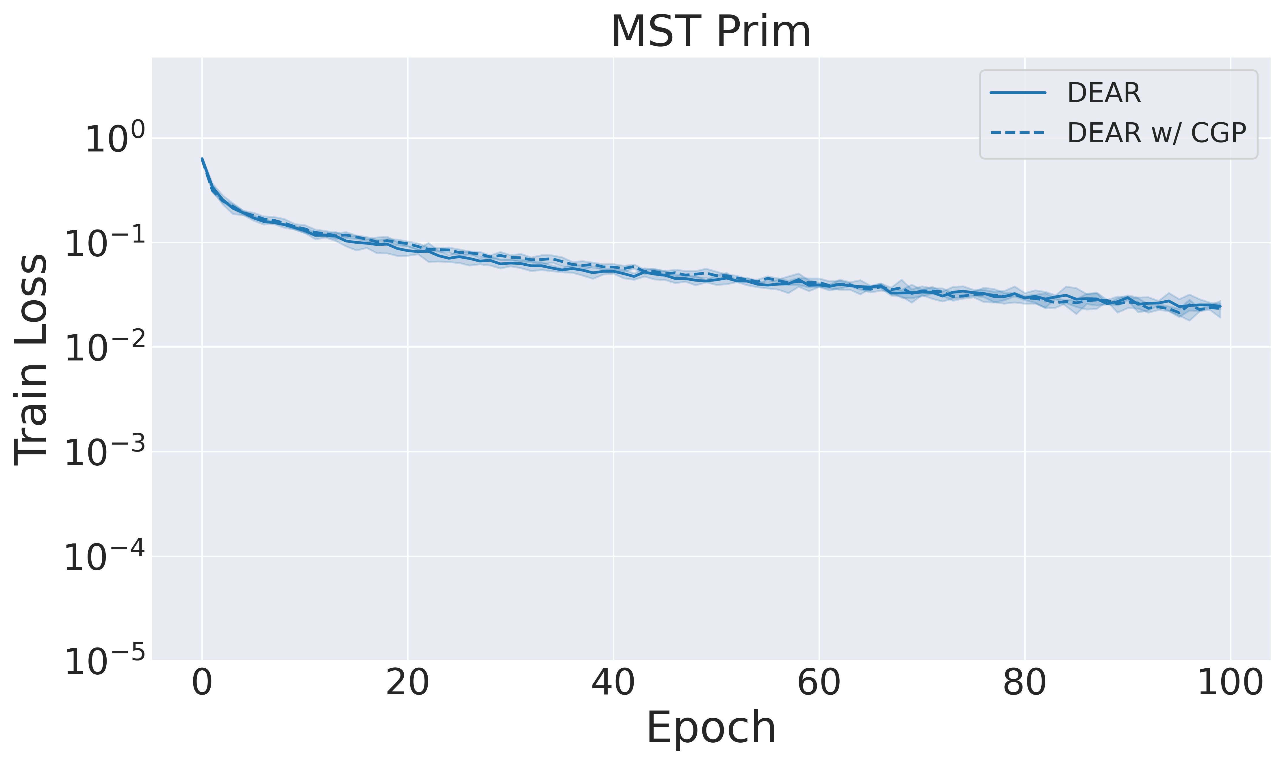
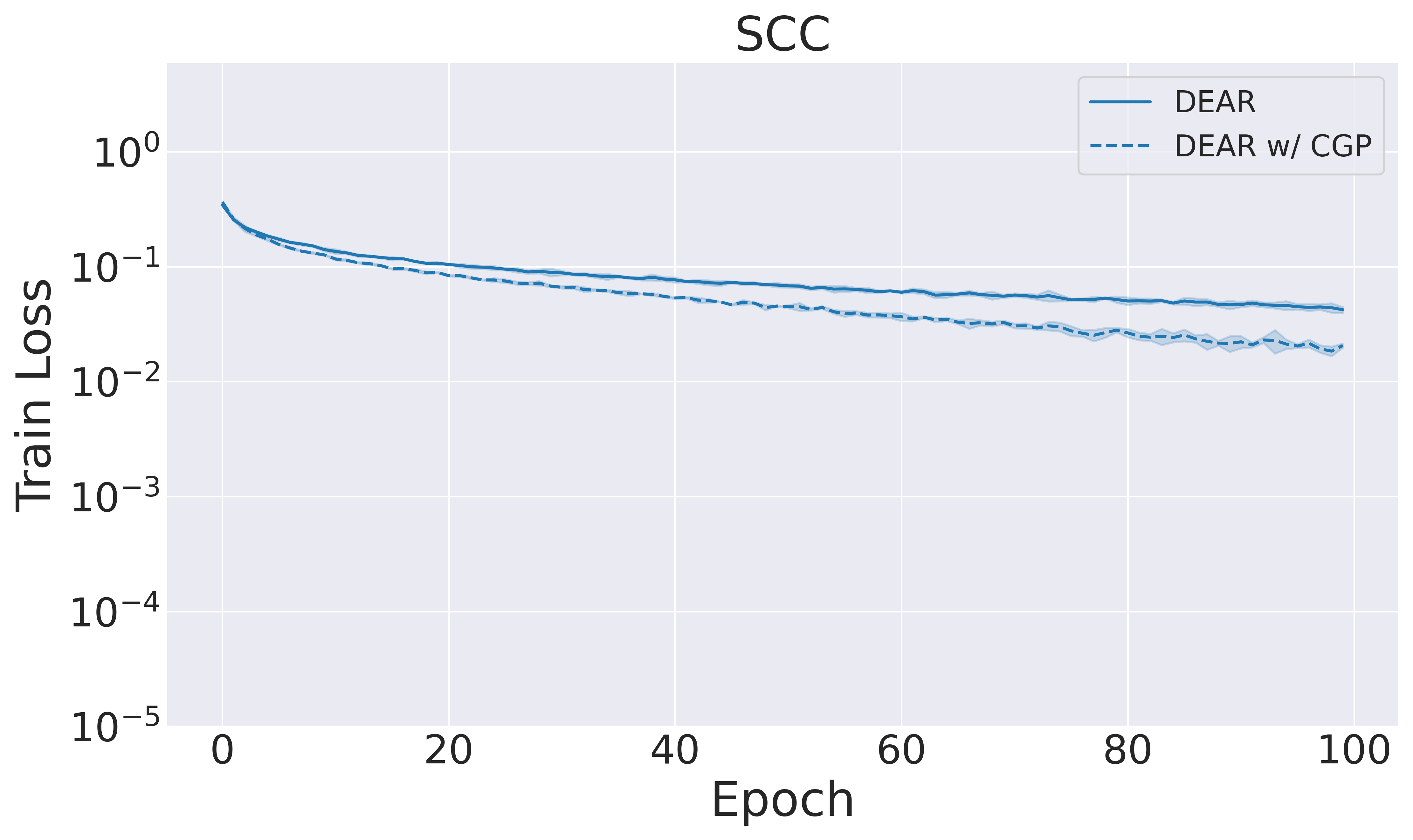
Figure 7: Effect of using Cayley Graph propagation on the train loss.

Appendix J Alignment gives closer convergence

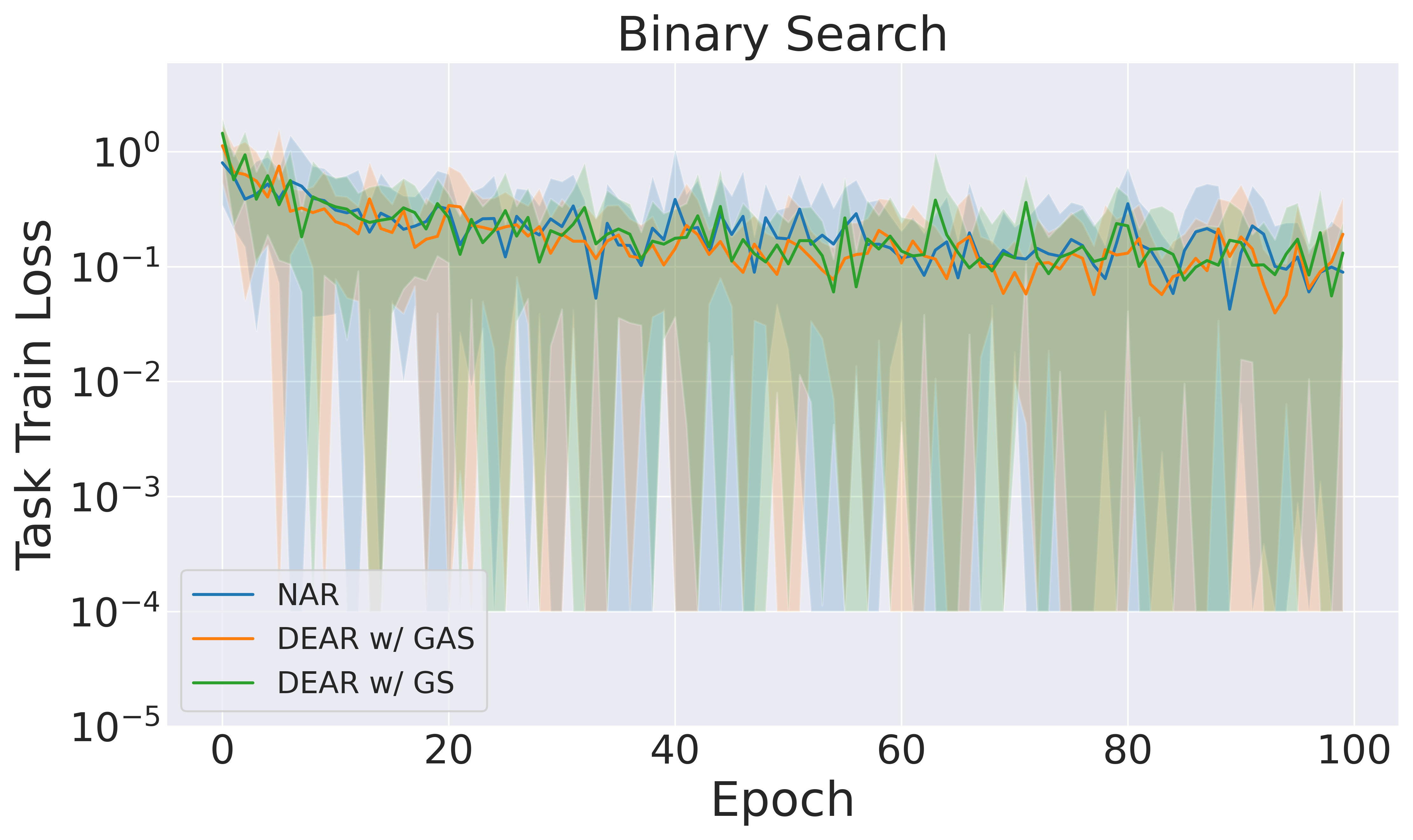
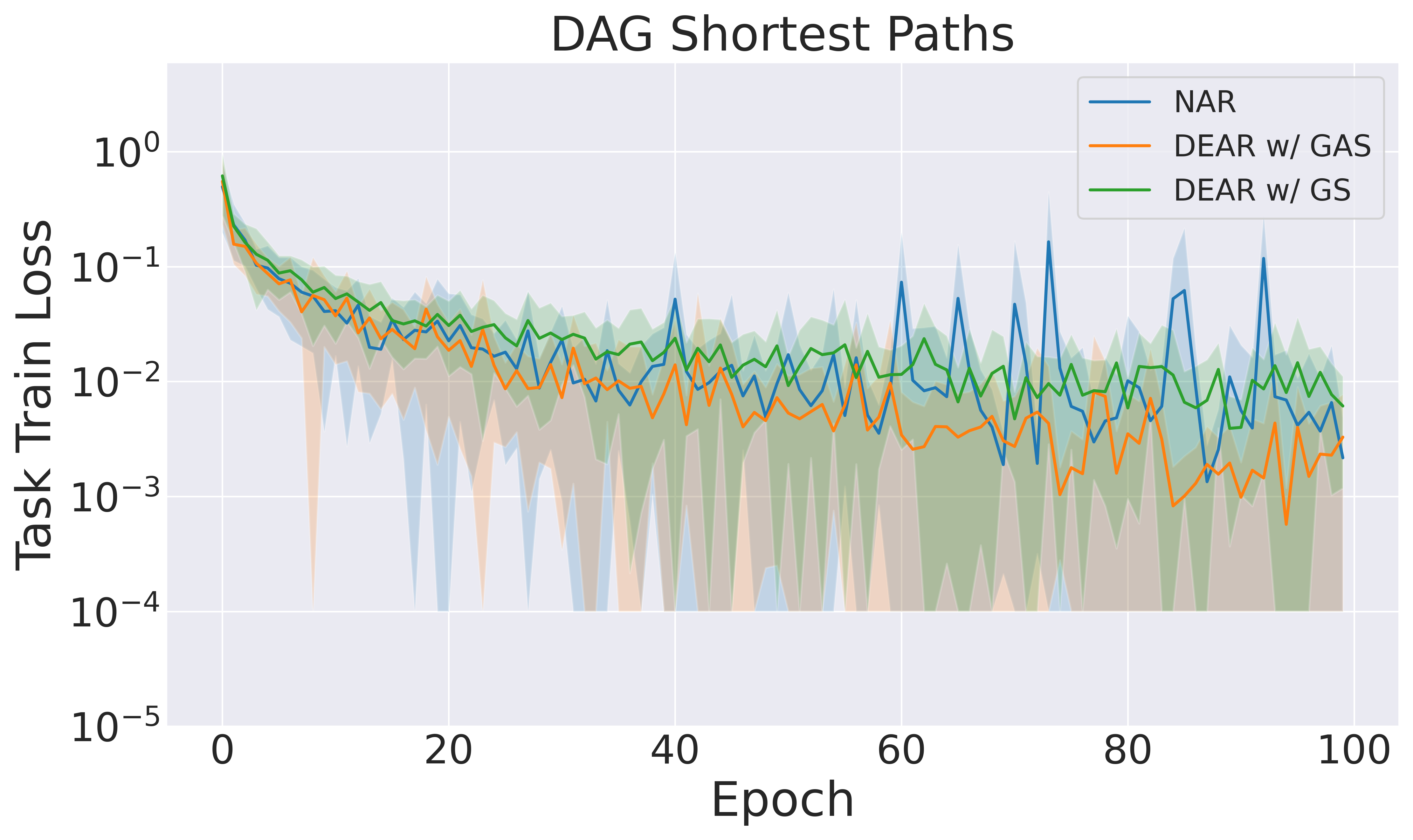
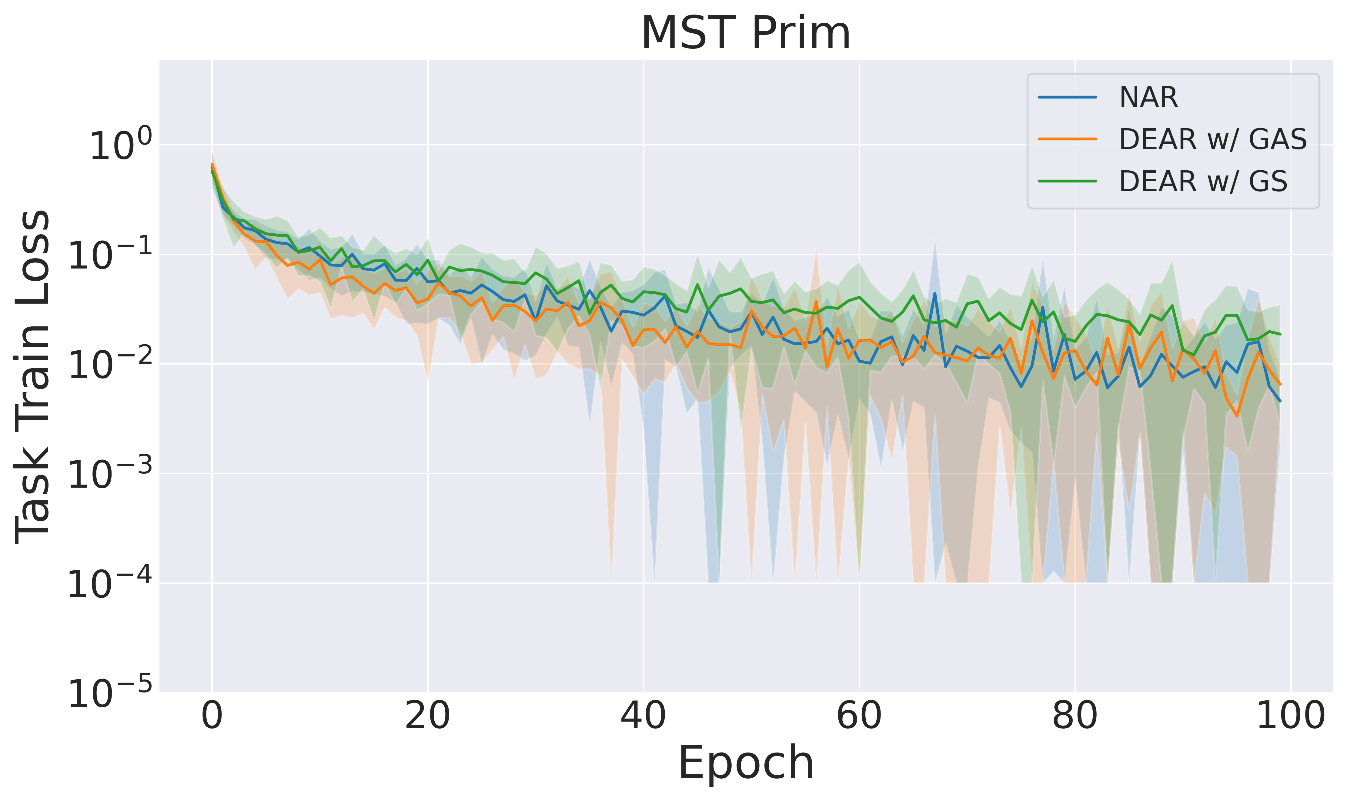
Figure 8: Alignment (orange) leads to lower task train loss compared to no aligment, but using stochasticity and GRANOLA (green).

References

- Alon and Yahav, [2020] Alon, U. and Yahav, E. (2020). On the bottleneck of graph neural networks and its practical implications. arXiv preprint arXiv:2006.05205.
- Anderson, [1965] Anderson, D. G. (1965). Iterative procedures for nonlinear integral equations. Journal of the ACM ( JACM).
- Arnaiz-Rodríguez et al., [2022] Arnaiz-Rodríguez, A., Begga, A., Escolano, F., and Oliver, N. (2022). Diffwire: Inductive graph rewiring via the Lovàsz bound. arXiv preprint arXiv:2206.07369.
- Bai et al., [2019] Bai, S., Kolter, J. Z., and Koltun, V. (2019). Deep equilibrium models. Neural Information Processing Systems.
- Bai et al., [2021] Bai, S., Koltun, V., and Kolter, J. Z. (2021). Stabilizing equilibrium models by jacobian regularization. International Conference on Machine Learning.
- Banerjee et al., [2022] Banerjee, P. K., Karhadkar, K., Wang, Y. G., Alon, U., and Montúfar, G. (2022). Oversquashing in gnns through the lens of information contraction and graph expansion. In 2022 58th Annual Allerton Conference on Communication, Control, and Computing (Allerton), pages 1–8. IEEE.
- Barbero et al., [2024] Barbero, F., Velingker, A., Saberi, A., Bronstein, M. M., and Giovanni, F. D. (2024). Locality-aware graph rewiring in GNNs. In The Twelfth International Conference on Learning Representations.
- Bevilacqua et al., [2023] Bevilacqua, B., Nikiforou, K., Ibarz, B., Bica, I., Paganini, M., Blundell, C., Mitrovic, J., and Velickovic, P. (2023). Neural algorithmic reasoning with causal regularisation. International Conference on Machine Learning, ICML 2023, 23-29 July 2023, Honolulu, Hawaii, USA, 202:2272–2288.
- Broyden, [1965] Broyden, C. G. (1965). A class of methods for solving nonlinear simultaneous equations. Mathematics of Computation, 19:577–593.
- Cai et al., [2023] Cai, C., Hy, T. S., Yu, R., and Wang, Y. (2023). On the connection between mpnn and graph transformer. In International Conference on Machine Learning, pages 3408–3430. PMLR.
- Cormen et al., [2009] Cormen, T. H., Leiserson, C. E., Rivest, R. L., and Stein, C. (2009). Introduction to Algorithms, 3rd Edition. MIT Press.
- Deac et al., [2022] Deac, A., Lackenby, M., and Veličković, P. (2022). Expander graph propagation. In Learning on Graphs Conference, pages 38–1. PMLR.
- Dudzik and Veličković, [2022] Dudzik, A. J. and Veličković, P. (2022). Graph neural networks are dynamic programmers. Advances in Neural Information Processing Systems, 35:20635–20647.
- Dudzik et al., [2024] Dudzik, A. J., von Glehn, T., Pascanu, R., and Veličković, P. (2024). Asynchronous algorithmic alignment with cocycles. In Villar, S. and Chamberlain, B., editors, Proceedings of the Second Learning on Graphs Conference, volume 231 of Proceedings of Machine Learning Research, pages 3:1–3:17. PMLR.
- Eliasof et al., [2024] Eliasof, M., Bevilacqua, B., Schönlieb, C.-B., and Maron, H. (2024). Granola: Adaptive normalization for graph neural networks. arXiv preprint arXiv: 2404.13344.
- Engelmayer et al., [2023] Engelmayer, V., Georgiev, D. G., and Veličković, P. (2023). Parallel algorithms align with neural execution. In The Second Learning on Graphs Conference.
- Erdős et al., [1960] Erdős, P., Rényi, A., et al. (1960). On the evolution of random graphs. Publ. Math. Inst. Hung. Acad. Sci, 5(1):17–60.
- Fiore, [2324] Fiore, M. (2023/24). Denotational Semantics. Lecture notes for Part II of the Computer Science Tripos. University of Cambridge.
- Geng and Kolter, [2023] Geng, Z. and Kolter, J. Z. (2023). Torchdeq: A library for deep equilibrium models. https://github.com/locuslab/torchdeq.
- Ghaoui et al., [2019] Ghaoui, L., Gu, F., Travacca, B., Askari, A., and Tsai, A. Y. (2019). Implicit deep learning. SIAM Journal on Mathematics of Data Science.
- Gilmer et al., [2017] Gilmer, J., Schoenholz, S. S., Riley, P. F., Vinyals, O., and Dahl, G. E. (2017). Neural message passing for quantum chemistry. In International conference on machine learning, pages 1263–1272. PMLR.
- Giovanni et al., [2023] Giovanni, F. D., Rusch, T. K., Bronstein, M. M., Deac, A., Lackenby, M., Mishra, S., and Veličković, P. (2023). How does over-squashing affect the power of gnns? arXiv preprint arXiv: 2306.03589.
- Gunter, [1992] Gunter, C. A. (1992). Semantics of programming languages: structures and techniques. MIT press.
- Hamrick et al., [2018] Hamrick, J. B., Allen, K. R., Bapst, V., Zhu, T., McKee, K. R., Tenenbaum, J. B., and Battaglia, P. W. (2018). Relational inductive bias for physical construction in humans and machines. arXiv preprint arXiv:1806.01203.
- Harris and Ross, [1955] Harris, T. and Ross, F. (1955). Fundamentals of a method for evaluating rail net capacities. Technical report.
- Hu et al., [2021] Hu, W., Fey, M., Ren, H., Nakata, M., Dong, Y., and Leskovec, J. (2021). Ogb-lsc: A large-scale challenge for machine learning on graphs. arXiv preprint arXiv:2103.09430.
- Hu et al., [2020] Hu, W., Fey, M., Zitnik, M., Dong, Y., Ren, H., Liu, B., Catasta, M., and Leskovec, J. (2020). Open graph benchmark: Datasets for machine learning on graphs. Advances in neural information processing systems, 33:22118–22133.
- Hwang et al., [2022] Hwang, E., Thost, V., Dasgupta, S. S., and Ma, T. (2022). An analysis of virtual nodes in graph neural networks for link prediction. In The First Learning on Graphs Conference.
- Ibarz et al., [2022] Ibarz, B., Kurin, V., Papamakarios, G., Nikiforou, K., Bennani, M., Csordás, R., Dudzik, A. J., Bosnjak, M., Vitvitskyi, A., Rubanova, Y., Deac, A., Bevilacqua, B., Ganin, Y., Blundell, C., and Velickovic, P. (2022). A generalist neural algorithmic learner. In Rieck, B. and Pascanu, R., editors, Learning on Graphs Conference, LoG 2022, 9-12 December 2022, Virtual Event, volume 198 of Proceedings of Machine Learning Research, page 2. PMLR.
- Karhadkar et al., [2022] Karhadkar, K., Banerjee, P. K., and Montúfar, G. (2022). Fosr: First-order spectral rewiring for addressing oversquashing in gnns. arXiv preprint arXiv:2210.11790.
- Kingma and Ba, [2015] Kingma, D. P. and Ba, J. (2015). Adam: A method for stochastic optimization. In Bengio, Y. and LeCun, Y., editors, 3rd International Conference on Learning Representations, ICLR 2015, San Diego, CA, USA, May 7-9, 2015, Conference Track Proceedings.
- Kolter et al., [2023] Kolter, Z., Duvenaud, D., and Johnson, M. (2023). Deep equilibrium models (deq) tutorial. https://implicit-layers-tutorial.org/deep_equilibrium_models/. Accessed: 2024-08-27.
- Liu et al., [2024] Liu, J., Hooi, B., Kawaguchi, K., Wang, Y., Dong, C., and Xiao, X. (2024). Scalable and effective implicit graph neural networks on large graphs. In The Twelfth International Conference on Learning Representations.
- Mahdavi et al., [2023] Mahdavi, S., Swersky, K., Kipf, T., Hashemi, M., Thrampoulidis, C., and Liao, R. (2023). Towards better out-of-distribution generalization of neural algorithmic reasoning tasks. Transactions on Machine Learning Research.
- Mohar, [1991] Mohar, B. (1991). Eigenvalues, diameter, and mean distance in graphs. Graphs and combinatorics, 7(1):53–64.
- Paszke et al., [2019] Paszke, A., Gross, S., Massa, F., Lerer, A., Bradbury, J., Chanan, G., Killeen, T., Lin, Z., Gimelshein, N., Antiga, L., et al. (2019). Pytorch: An imperative style, high-performance deep learning library. arXiv preprint arXiv:1912.01703.
- Rodionov and Prokhorenkova, [2023] Rodionov, G. and Prokhorenkova, L. (2023). Neural algorithmic reasoning without intermediate supervision. arXiv preprint arXiv:2306.13411.
- Scott, [1982] Scott, D. S. (1982). Domains for denotational semantics. In Automata, Languages and Programming: Ninth Colloquium Aarhus, Denmark, July 12–16, 1982 9, pages 577–610. Springer.
- Scott and Strachey, [1971] Scott, D. S. and Strachey, C. (1971). Toward a mathematical semantics for computer languages, volume 1. Oxford University Computing Laboratory, Programming Research Group Oxford.
- Sharir, [1981] Sharir, M. (1981). A strong-connectivity algorithm and its applications in data flow analysis. Computers & Mathematics with Applications, 7(1):67–72.
- Shirzad et al., [2023] Shirzad, H., Velingker, A., Venkatachalam, B., Sutherland, D. J., and Sinop, A. K. (2023). Exphormer: Sparse transformers for graphs. In International Conference on Machine Learning, pages 31613–31632. PMLR.
- Tang et al., [2020] Tang, H., Huang, Z., Gu, J., Lu, B.-L., and Su, H. (2020). Towards scale-invariant graph-related problem solving by iterative homogeneous gnns. Advances in Neural Information Processing Systems, 33.
- Tarski, [1955] Tarski, A. (1955). A lattice-theoretical fixpoint theorem and its applications.
- Topping et al., [2021] Topping, J., Di Giovanni, F., Chamberlain, B. P., Dong, X., and Bronstein, M. M. (2021). Understanding over-squashing and bottlenecks on graphs via curvature. arXiv preprint arXiv:2111.14522.
- Veličković et al., [2022] Veličković, P., Badia, A. P., Budden, D., Pascanu, R., Banino, A., Dashevskiy, M., Hadsell, R., and Blundell, C. (2022). The clrs algorithmic reasoning benchmark. In International Conference on Machine Learning, pages 22084–22102. PMLR.
- [46] Velickovic, P. and Blundell, C. (2021a). Neural algorithmic reasoning. Patterns, 2(7):100273.
- [47] Velickovic, P. and Blundell, C. (2021b). Neural algorithmic reasoning. Patterns, 2(7):100273.
- Veličković et al., [2020] Veličković, P., Buesing, L., Overlan, M., Pascanu, R., Vinyals, O., and Blundell, C. (2020). Pointer graph networks. Advances in Neural Information Processing Systems, 33:2232–2244.
- Veličković et al., [2020] Veličković, P., Ying, R., Padovano, M., Hadsell, R., and Blundell, C. (2020). Neural execution of graph algorithms. In 8th International Conference on Learning Representations, ICLR 2020, Addis Ababa, Ethiopia, April 26-30, 2020. OpenReview.net.
- Veličković, [2023] Veličković, P. (2023). Neural algorithmic reasoning. The Gradient.
- Wilson et al., [2024] Wilson, J., Bechler-Speicher, M., and Veličković, P. (2024). Cayley graph propagation. arXiv preprint arXiv:2410.03424.
- Winskel, [1993] Winskel, G. (1993). The formal semantics of programming languages: an introduction. MIT press.
- Xhonneux et al., [2024] Xhonneux, S., He, Y., Deac, A., Tang, J., and Gidel, G. (2024). Deep equilibrium models for algorithmic reasoning. In ICLR Blogposts 2024. https://iclr-blogposts.github.io/2024/blog/deqalg-reasoning/.
- Xu et al., [2018] Xu, K., Li, C., Tian, Y., Sonobe, T., Kawarabayashi, K.-i., and Jegelka, S. (2018). Representation learning on graphs with jumping knowledge networks. In International conference on machine learning, pages 5453–5462. PMLR.
- Xu et al., [2020] Xu, K., Li, J., Zhang, M., Du, S. S., ichi Kawarabayashi, K., and Jegelka, S. (2020). What can neural networks reason about? In International Conference on Learning Representations.