Asymptotic Time-Uniform Inference for Parameters in Averaged Stochastic Approximation
Abstract
We study time-uniform statistical inference for parameters in stochastic approximation (SA), which encompasses a bunch of applications in optimization and machine learning. To that end, we analyze the almost-sure convergence rates of the averaged iterates to a scaled sum of Gaussians in both linear and nonlinear SA problems. We then construct three types of asymptotic confidence sequences that are valid uniformly across all times with coverage guarantees, in an asymptotic sense that the starting time is sufficiently large. These coverage guarantees remain valid if the unknown covariance matrix is replaced by its plug-in estimator, and we conduct experiments to validate our methodology.
1 Introduction
Traditional statistical inference for parameters is based on asymptotic/non-asymptotic coverage guarantees at fixed sample sizes. Such guarantees tend to become problematic in sequential experimental design due to the issue of “peeking”, i.e., experimenters deciding whether to collect more data for further experiments after looking at current results in order to make the outcome more significant (Feller,, 1940; Anscombe,, 1954; Robbins,, 1952). Recently, there has been an emerging literature on safe anytime-valid inference (Johari et al.,, 2022; Howard et al.,, 2021; Grünwald et al.,, 2020; Shafer,, 2021; Pace and Salvan,, 2020; Ramdas et al.,, 2023) that partially solve such problems. At a high level, they utilize a supermartingale method coupled with Ville’s inequality (Ville,, 1939) to obtain time-uniform coverage guarantees for the quantities of interest, which is also equivalent to coverage guarantees for arbitrary stopping times (Ramdas et al.,, 2020):
With such guarantees, the corresponding statistical inference procedure remains valid even in the presence of peeking, since the experimenter’s decision of whether to stop conducting further experiments can always be regarded as a stopping time. This technique has been applied to a series of traditional statistical tasks including mean estimation and hypothesis tests (Darling and Robbins,, 1968; Howard et al.,, 2021; Waudby-Smith and Ramdas,, 2024; Ramdas et al.,, 2023).
This work takes a step forward to study time-uniform statistical inference in the stochastic approximation (SA) framework, which refers to a wide class of online iterative algorithms and is prevalent in modern machine learning applications such as stochastic gradient descent (SGD) and reinforcement learning (RL) due to memory and efficiency superiority over offline methods. Specifically, the SA iterates follow the recursive stochastic updates as (2.1) below. Despite recent progress on statistical inference for SA (Chen et al.,, 2020; Fang et al.,, 2018; Su and Zhu,, 2023; Lee et al.,, 2022), none of them provide time-uniform results and therefore they still suffer from the peeking issue. The goal of this paper is to provide asymptotic time-uniform coverage guarantees of the following form:
where is the averaged iterate and is the true parameter. As a direct consequence, for sequential experiments on e-commerce platforms or in clinical trials where the parameters of interest are updated iteratively, our results provide confidence sequences for the true parameter with asymptotically valid error control regardless of the data collection strategy of experimenters.
1.1 Our Contributions
Our theoretical contributions mainly lie in the following three parts.
-
(i)
We establish an almost-sure Gaussian approximation result for the averaged iterates to a scaled sum of i.i.d. Gaussians with precise convergence rates (Theorem 3.1), and provide a refined analysis on the relationship between the hyperparameters and these rates (Section 3.2) as well as the optimal rates (Section 3.3) in both linear and nonlinear cases.
-
(ii)
We devise three confidence sequence boundaries for the scaled sum of i.i.d. Gaussians and provide time-uniform coverage guarantees (Section 4.1).
-
(iii)
For practical inference, we derive the almost-sure convergence for the plug-in estimator of the unknown covariance matrix that is used in constructing confidence sequences (Section 4.2), and prove that asymptotic time-uniform coverage guarantees still hold when replacing this covariance matrix with its plug-in analogue (Section 4.3).
We perform numerical experiments in Section 5 to validate our methodology. Our idea stems from the time-uniform central limit theory proposed in Waudby-Smith et al., (2021), which highlights the necessity of “almost-sure” convergence of all quantities of interest, instead of usual “in-probability” or “in-law” ones. This requirement leads us to derive brand new convergence results mentioned above in the SA framework.
1.2 Related Work
Anytime-valid inference.
The idea of confidence sequences is initiated by Darling and Robbins, (1967), which provided a sequential estimation approach for the median. A more recent work Howard et al., (2021) gave comprehensive analysis and constructions of confidence sequences for the mean based on time-uniform concentration bounds from Howard et al., (2020). Similar techniques were adopted in Howard and Ramdas, (2022) for quantile estimation and in Waudby-Smith and Ramdas, (2024) for bounded mean estimation. Another line of research, nonparametric sequential testing, goes back to Wald, (1945). Based on the test martingale method from Shafer et al., (2011), Grünwald et al., (2020) developed a theory of safe hypothesis testing and proposed general methods for constructing tests with optimal powers. Subsequent works include Ramdas et al., (2020) for testing symmetry, Ramdas et al., (2022) for testing exchangeability, etc.
Statistical inference for stochastic approximation.
Based on the seminal work of Polyak and Juditsky, (1992), Chen et al., (2020) studied asymptotic normality of averaged iterates from SGD, and proposed the plug-in and batch-means estimators for the asymptotic covariance matrix in order to perform statistical inference on model parameters. Zhu et al., (2023) developed a fully online batch-means method which improves computation and memory efficiency over the original one in Chen et al., (2020). Fang et al., (2018) proposed an online bootstrap procedure for the estimation of confidence intervals via a number of randomly perturbed SGD iterates. Su and Zhu, (2018) designed a hierarchical incremental gradient descent method termed HiGrad that hierarchically split SGD updates into multiple threads and constructed a -based confidence interval for the parameter. Lee et al., (2022) leveraged insights from time series regression in econometrics (Abadir and Paruolo,, 1997; Kiefer et al.,, 2000) and constructed asymptotic pivotal statistics for parameter inference via random scaling, which was extended to different machine learning scenarios in Li et al., (2022); Li et al., 2023b ; Li et al., 2023a . Chen et al., 2021a ; Chen et al., 2021b ; Chen et al., (2022) studied online statistical inference in the contextual bandit settings and analyzed the performance and efficiency of weighted versions of SGD.
2 Problem Setup
We begin by introducing the problem setup. We are concerned with solving the root-finding problem , where is expressed as an expectation over the data point ; i.e., . Supposing we only have access to a sequence of i.i.d. data points , a typical stochastic approximation (SA) algorithm is given by the following -dimensional recursion:
| (2.1) |
Starting from an initializer , the iterates will converge to the unique root and possess favorable statistical properties under certain assumptions that we are about to display.
Assumption 2.1 (Lyapunov function).
There exist a differentiable function and a constant such that for all and , the following conditions hold.
-
(i)
.
-
(ii)
for some .
-
(iii)
for some .
-
(iv)
for .
-
(v)
for some .
Assumption 2.2 (Local linearity).
There exist a matrix and constants , , such that for all ,
and that for all , where denotes the -th eigenvalue.
Assumption 2.3 (Lipschitzness).
There exists a constant such that for any ,
Assumption 2.4 (Step size).
The step size is for some constant .
Assumption 2.5 (Noise).
For each , let . The martingale difference sequence satisfies the following conditions.
-
(i)
For all , almost surely for some constant .
-
(ii)
The following decomposition holds: , where
-
(a)
almost surely;
-
(b)
as , where is a symmetric and positive definite matrix;
-
(c)
as ;
-
(d)
for all large enough, almost surely, where as .
-
(a)
-
(iii)
For all , and for some constants and .
Remark 2.1.
Assumptions 2.1-2.5 are analogous to Assumptions 3.1-3.4 of Polyak and Juditsky, (1992), which are standard in the SA literature. Assumptions 2.1-2.3 are restrictions on and to ensure convergence of the SA algorithm (2.1). In Assumption 2.4 we use a standard polynomial step size schedule that satisfies the Robbins-Monro conditions (Robbins and Monro,, 1951), i.e., and . Assumption 2.5 contains conditions on the scale of noise and is essential to establishing the asymptotic behavior of the averaged iterates. The SA framework includes a bunch of examples including linear regression and logistic regression, which are studied in our experiments (Section 5).
3 Almost-Sure Gaussian Approximation
In the following Theorem 3.1, we approximate the averaged iterate by a sum of i.i.d. Gaussians in an almost-sure sense, and characterize the corresponding approximation rate. Its detailed proof is deferred to Appendix A.1.
Theorem 3.1 (Gaussian approximation).
Compared with the (functional) central limit theorems for averaged iterates in the literature (Polyak and Juditsky,, 1992; Chen et al.,, 2020, 2024; Lee et al.,, 2022, 2024; Chen et al.,, 2023; Li et al.,, 2022; Li et al., 2023b, ; Li et al., 2023a, ), our Theorem 3.1 provides an almost-sure version instead of a usual in-probability one under some mildly stronger assumptions (see Assumption 3.1 below). In addition, we precisely characterize the approximation rate when , while previous works only verify that it is of order for the sole purpose of establishing asymptotic normality.
3.1 Proof Idea of Theorem 3.1
The high-level idea of its proof is to decompose into the following five parts (Polyak and Juditsky,, 1992): denoting , , and , we have
Here, can be regarded as an approximation of . Below we discuss how the different rates contained in and appear from the above five error terms.
Put simply, is the error caused by inaccurate initialization and is of order . And is the error induced when we linearize the expected increment of an update (2.1) by . By Assumption 2.2, when is close to (which is always true when ), this linearization error will decay at a rate similar to that of , and we rigorously prove it is of order in Lemma A.1.
characterizes the approximation error of to and is of order , as also proved in Lemma A.1. Compared to the corresponding proof in Polyak and Juditsky, (1992) (see Lemma 2 and the proof of Theorem 1 therein), in order for the almost-sure convergence rate of to be faster than , we additionally need a finite -th moment condition on the noise, which we formulate as Assumption 2.5 (iii). This condition also appears in previous works (Zhu and Dong,, 2021; Lee et al.,, 2022; Li et al.,, 2022; Li et al., 2023a, ) concerning weak convergence of the scaled iterates to a Brownian motion (i.e., functional central limit theorems), and is also essential to our proof.
characterizes the error induced when we calibrate the increments of the martingale to i.i.d. random variables, sharing the same randomness and the same limiting covariance . This is easily achieved by considering the martingale . Using the averaged Lipschitzness in Assumption 2.3, again we link the convergence rate of to that of and derive a rate of in Lemma A.2.
Finally, is approximated by i.i.d. Gaussians with the same mean and covariance, using almost-sure invariance principles from Strassen, (1967); Philipp, (1986). For one-dimensional SA problems with , the approximation error is of order (Strassen,, 1967). For high-dimensional SA problems with , the error rate is slightly worsened to (Philipp,, 1986).
Combining the convergence rates of the above five parts finally yields the overall strong approximation rate for arbitrarily small .
3.2 Rate Analysis
Based on Theorem 3.1, we now perform a detailed analysis on the behavior of approximation rates. In Figure 3.1 below, we plot the negative exponents of these rates separately with respect to (which is the negative exponent of the step size as defined in Assumption 2.4) for both linear and nonlinear SA problems, resulting in several new findings.
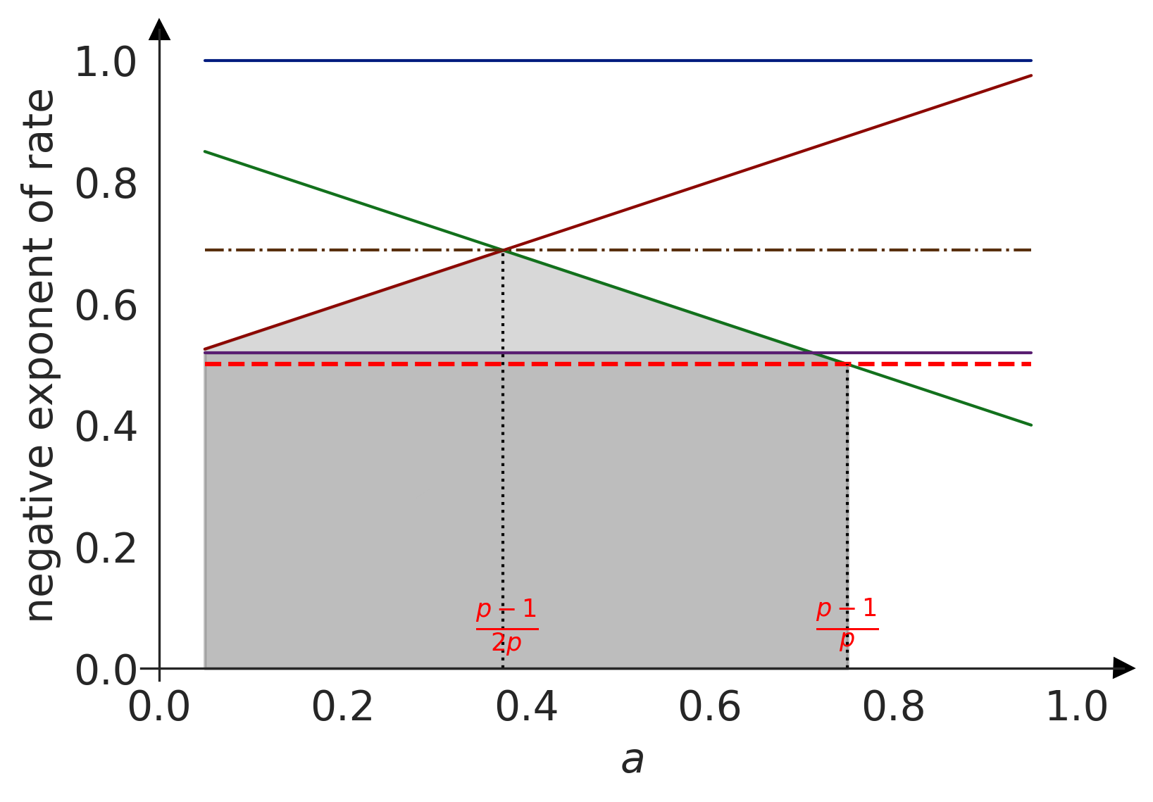
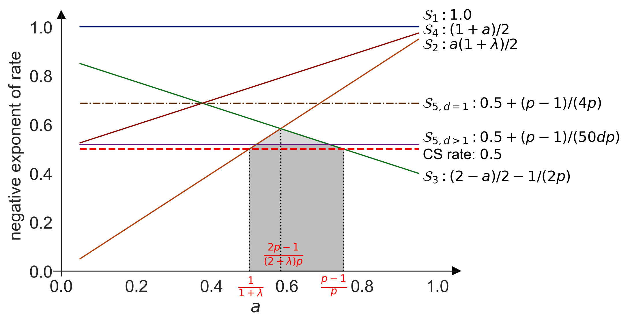
Firstly, the linearization error and the covariance calibration error decay faster for larger , while the matrix-inverse approximation error decays slower for larger . This is due to the fact that both and are controlled by the error . For large , gets very close to so the variance of the iterate dominates its bias in . Since its variance is proportional to that of the increment in (2.1), it follows that larger implies smaller and thus faster convergence of (see Lemma C.3 for details). On the other hand, purely depends on the approximation rate of to , which is unrelated to the randomness in data points . From the definition of as well as Lemma C.5, smaller will, on the contrary, impede the convergence of .
Secondly, we hope the overall approximation rate to be of order , so that the invariance principle and the law of the iterated logarithm for will also hold for . To meet this requirement, the rate of step sizes must satisfy in the linear case and in the nonlinear case, the latter of which implicitly requires . In the special case where and , the feasible range for becomes and , respectively, matching the corresponding conditions in the literature (Polyak and Juditsky,, 1992). In the sequel, we add these conditions for to pave the way for further development of time-uniform inference.
Assumption 3.1 (Rate condition).
The constants satisfy one of the following conditions:
-
(i)
(Linear SA) and .
-
(ii)
(Nonlinear SA) and .
3.3 Optimal Approximation Rates
In this section, we study the best possible approximation rate of the overall errors in Theorem 3.1. Note that stems from the existing almost-sure invariance principles (Strassen,, 1967; Philipp,, 1986) that are generally hard to improve, so we mainly focus on improving . According to Figure 3.1, for linear SA problems, the best possible approximation rate is attained at , in which case ; for nonlinear SA problems, the best possible approximation rate is attained at , in which case . In the special case where and , the optimal approximation rate becomes for the linear case and for the nonlinear case, respectively. These are brand new results that characterize the almost-sure convergence rates of the averaged iterates to a scaled sum of i.i.d. random vectors:
| (3.1) |
Corollary 3.2 (Linear SA).
4 Construction of Asymptotic Confidence Sequences
Having established the almost-sure Gaussian approximation result, it is reasonable to believe that confidence sequences for the well-behaved sum of Gaussians will also serve as confidence sequences for the averaged iterates in some asymptotic sense, since as the above two behaves quite the same except for negligible terms. In this section, we follow this idea to design such asymptotic confidence sequences for the averaged iterates, and provide suitable error guarantees for them.
4.1 Confidence Sequences for the Approximating Process
We consider three different types of confidence sequences for the mean of multivariate Gaussians, which serve as building blocks for time-uniform inference on averaged iterates. Their specific forms are displayed in Table 4.1, where we denote as the mean of -dimensional i.i.d. Gaussian random vectors with mean zero and covariance . Detailed derivation is deferred to Appendix B.
| Notation | Form | Reference |
|---|---|---|
| Howard et al., (2021) Eq. 3.4 | ||
| Howard et al., (2021) Eq. 3.7 | ||
| Whitehouse et al., (2023) Cor. 4.3 | ||
LIL boundary with union bounds, .
This bound comes from Equation 3.4 of Howard et al., (2021), which is called the law of the iterated logarithm (LIL) boundary because this boundary scales as . To accommodate the multivariate case in out settings, we use a union bound over dimensions of the standardized process , which results in a -type confidence sequence (see Appendix B.2 for details).
Gaussian mixture boundary, .
This -type bound comes from Equation 3.7 of Howard et al., (2021) and originally dates back to Robbins and Siegmund, (1970); Lai, (1976). In the formula of , is a user-specified time, and where is the lower branch of the Lambert function, i.e., the most negative real-valued solution in to . Such specific form of results in the minimal volume of the confidence region at time among all Gaussian mixture boundaries (see Appendix B.3 for details).
LIL boundary with -nets, .
This -type bound comes from Whitehouse et al., (2023) and scales as . Unlike the union bound technique used for , here is derived via the -net arguments (e.g., Chapter 5 of Wainwright, (2019)). The boundary contains a user-specified , the conditional number , and a constant . All other hyperparameters in the original form (Corollary 4.3 of Whitehouse et al., (2023)) are set to be the same as those in for ease of comparison (See Appendix B.4 for details).
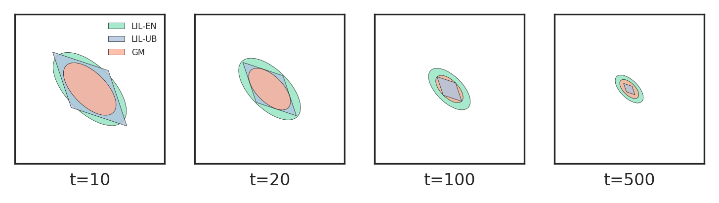
Figure 4.1 plots the above three confidence regions at different times in a 2D example. LIL-EN and GM boundaries are ellipsoids while LIL-UB boundaries are polygons. GM boundaries are generally smaller than LIL-UB boundaries when is small but larger when is large. This conforms to the rate of the former which grows faster than the rate of the latter. LIL-EN boundaries are always the largest in this illustration.
The following Proposition 4.1 formally states the time-uniform coverage property for these confidence sequences.
Proposition 4.1 (Time-Uniform Coverage for Gaussians).
Let be i.i.d. Gaussian random vectors with mean zero and covariance , and let . Then for any and any , it holds that
4.2 Almost-Sure Convergent Variance Estimator
The confidence sequences proposed in Section 4.1 all rely on the covariance , which is usually unknown a priori. Consequently, to construct practical confidence sequences for time-uniform inference, we need to design consistent estimators for in an online fashion. We mainly study the plug-in estimator (Chen et al.,, 2020), i.e., we estimate and with
and then use to approximate . Chen et al., (2020) proved convergence rates for and , but these are insufficient for proving asymptotic time-uniform coverage guarantees (Waudby-Smith et al.,, 2021). Instead, we need almost-sure convergence for these estimators, which we present below.
Assumption 4.1 (Unbiased estimate).
There exists a random function such that and for some .
Assumption 4.2 (Lipschitzness).
There exists a constant such that for any ,
4.3 Coverage Guarantees
Combining the pieces above, we arrive at the following coverage guarantee for the averaged iterates.
Theorem 4.4 (Asymptotic Time-Uniform Coverage).
As opposed to Proposition 4.1 where the coverage rate is above for time starting at the beginning, here we only have an “asymptotic” coverage rate when goes to infinity in order to compensate for the errors induced by Gaussian approximation and the plug-in error in covariance estimation. However, we show in experiments below that the coverage rate quickly becomes valid after iterations, which is just a warm start of the whole training process.
5 Experiments
In this section we run simulation experiments on two regression problems and illustrate the performance of three confidence sequences.
Linear regression.
For linear model , the loss function is , so the SGD update corresponds to (2.1) with . We assume , and generate data as and .
Logistic regression.
For logit model , the loss function is , so the SGD update corresponds to (2.1) with . We assume , and generate data as .
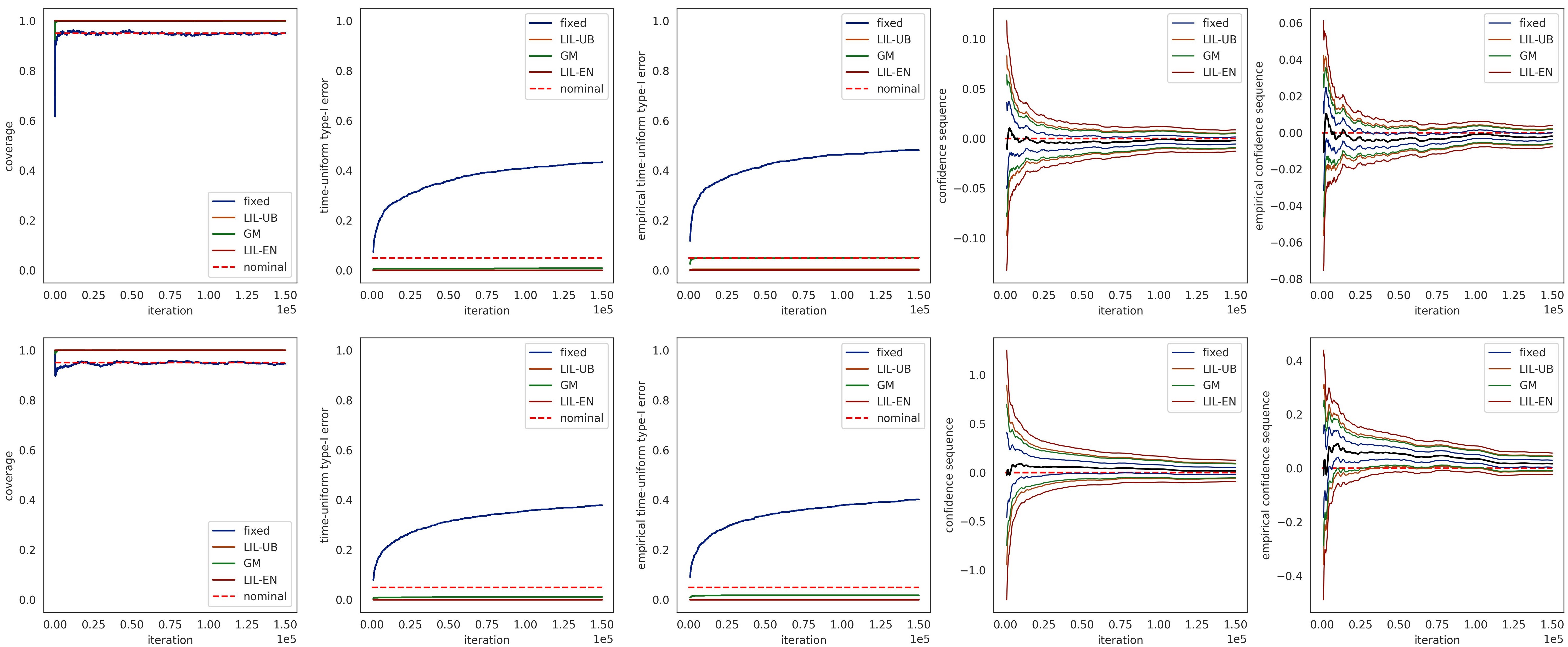
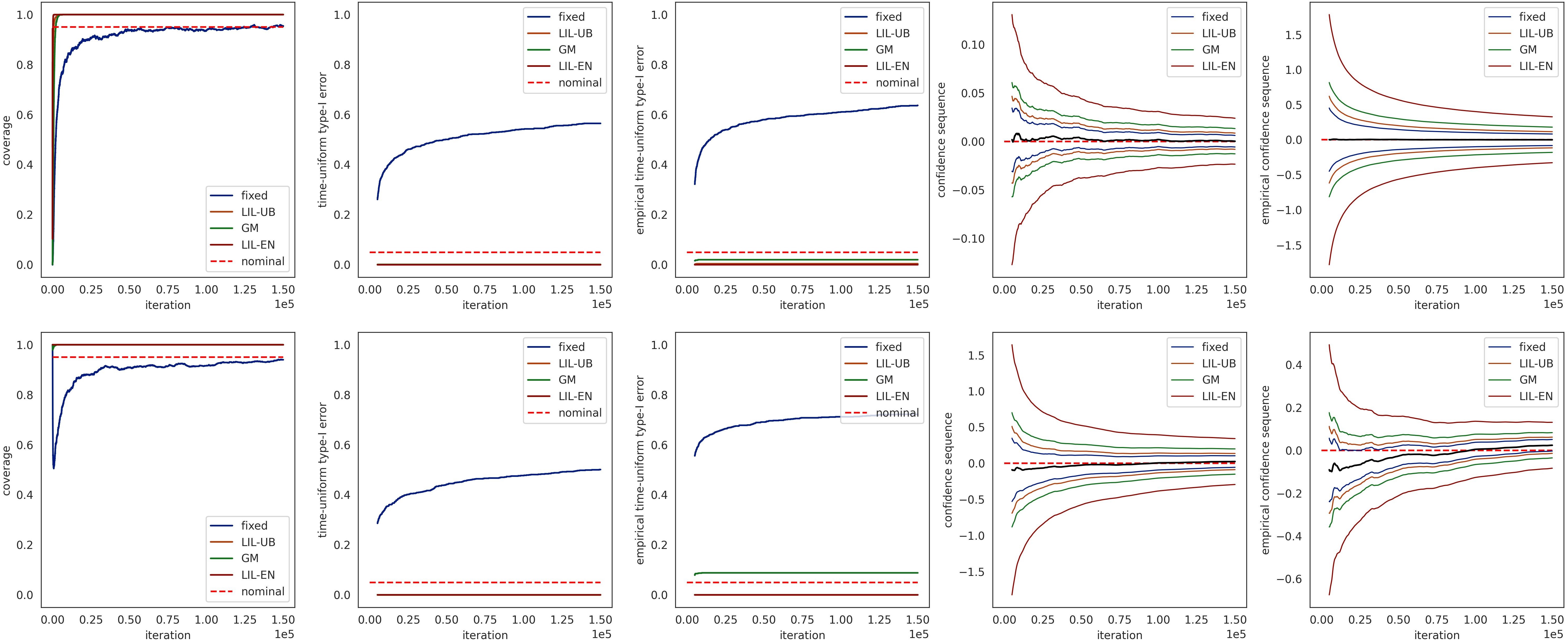
We conduct our experiment with Intel(R) Xeon(R) Gold 6132 CPU @ 2.60GHz. For each model, we perform SGD for iterations and repeat the trajectory for 1,000 times to compute coverage rates. We illustrate in Figures 5.1 and 5.2 the performance of three CSs as well as the traditional fixed-time CI when and , respectively. Specifically, we plot the fixed-time coverage rates at each iteration (Column 1), and the time-uniform coverage rates of the whole trajectory before each iteration (Column 2). To mitigate the effect of the approximation errors, we compute such time-uniform coverage rates starting from the 1,000-th iteration. We also plot the CS boundaries (Column 4), and their correspondences where the variance is replaced by its plug-in estimator (Column 3 and 5). As expected, our CSs are wider than the fixed-width one, and the latter fails to achieve the nominal time-uniform coverage rate. Comparing the boundaries of the CSs, we find the Gaussian mixture boundary (GM) is always the narrowest, achieving around two times of the fixed-time CI length. The boundary based on -nets is the widest and often achieves an extremely low coverage rate; this phenomenon is exacerbated in high dimensions. Nevertheless, all three CSs validate the asymptotic coverage guarantee.
6 Concluding Remarks
In this work we have leveraged probabilistic tools from anytime-valid inference to establish asymptotic confidence sequences for the averaged iterates from stochastic approximation algorithms. As a by-product, we have derived almost-sure convergence rates of the averaged iterates to a scaled sum of i.i.d. Gaussians, and discussed the trade-off between those rates from different causes as well as the best possible rate theoretically. We have proposed three asymptotic confidence sequences and established asymptotic type-I error control guarantees for them. Subsequent numerical experiments validate our results.
There are a few interesting directions for future work. The first is to extend our results to the martingale or Markovian noise settings so that algorithms such as bandit learning (Chen et al., 2021a, ; Chen et al., 2021b, ; Chen et al.,, 2022), policy gradient (Sutton et al.,, 1999) and actor-critic (Konda and Tsitsiklis,, 1999) can be fit into our framework. The second is to establish asymptotic confidence sequences for the last iterates (Pelletier,, 2000).
References
- Abadir and Paruolo, (1997) Abadir, K. M. and Paruolo, P. (1997). Two mixed normal densities from cointegration analysis. Econometrica: Journal of the Econometric Society, pages 671–680.
- Anscombe, (1954) Anscombe, F. J. (1954). Fixed-sample-size analysis of sequential observations. Biometrics, 10(1):89–100.
- Berning Jr, (1979) Berning Jr, J. A. (1979). On the multivariate law of the iterated logarithm. The Annals of Probability, 7(6):980–988.
- (4) Chen, H., Lu, W., and Song, R. (2021a). Statistical inference for online decision making: In a contextual bandit setting. Journal of the American Statistical Association, 116(533):240–255.
- (5) Chen, H., Lu, W., and Song, R. (2021b). Statistical inference for online decision making via stochastic gradient descent. Journal of the American Statistical Association, 116(534):708–719.
- Chen et al., (2022) Chen, X., Lai, Z., Li, H., and Zhang, Y. (2022). Online statistical inference for contextual bandits via stochastic gradient descent. arXiv preprint arXiv:2212.14883.
- Chen et al., (2024) Chen, X., Lai, Z., Li, H., and Zhang, Y. (2024). Online statistical inference for stochastic optimization via Kiefer-Wolfowitz methods. Journal of the American Statistical Association, 0(0):1–24.
- Chen et al., (2020) Chen, X., Lee, J. D., Tong, X. T., and Zhang, Y. (2020). Statistical inference for model parameters in stochastic gradient descent. The Annals of Statistics, 48(1):251–273.
- Chen et al., (2023) Chen, X., Lee, S., Liao, Y., Seo, M. H., Shin, Y., and Song, M. (2023). SGMM: Stochastic approximation to generalized method of moments. Journal of Financial Econometrics, page nbad027.
- Darling and Robbins, (1967) Darling, D. A. and Robbins, H. (1967). Confidence sequences for mean, variance, and median. Proceedings of the National Academy of Sciences, 58(1):66–68.
- Darling and Robbins, (1968) Darling, D. A. and Robbins, H. (1968). Some nonparametric sequential tests with power one. Proceedings of the National Academy of Sciences, 61(3):804–809.
- Durrett, (2019) Durrett, R. (2019). Probability: theory and examples, volume 49. Cambridge university press.
- Fang et al., (2018) Fang, Y., Xu, J., and Yang, L. (2018). Online bootstrap confidence intervals for the stochastic gradient descent estimator. Journal of Machine Learning Research.
- Feller, (1940) Feller, W. K. (1940). Statistical aspects of esp. The Journal of Parapsychology, 4(2):271.
- Grünwald et al., (2020) Grünwald, P., de Heide, R., and Koolen, W. M. (2020). Safe testing. In 2020 Information Theory and Applications Workshop (ITA), pages 1–54. IEEE.
- Hall and Heyde, (2014) Hall, P. and Heyde, C. C. (2014). Martingale limit theory and its application. Academic press.
- Howard and Ramdas, (2022) Howard, S. R. and Ramdas, A. (2022). Sequential estimation of quantiles with applications to a/b testing and best-arm identification. Bernoulli, 28(3):1704–1728.
- Howard et al., (2020) Howard, S. R., Ramdas, A., McAuliffe, J., and Sekhon, J. (2020). Time-uniform Chernoff bounds via nonnegative supermartingales. Probability Surveys, 17(none):257–317.
- Howard et al., (2021) Howard, S. R., Ramdas, A., McAuliffe, J., and Sekhon, J. (2021). Time-uniform, nonparametric, nonasymptotic confidence sequences. The Annals of Statistics, 49(2):1055–1080.
- Johari et al., (2022) Johari, R., Koomen, P., Pekelis, L., and Walsh, D. (2022). Always valid inference: Continuous monitoring of a/b tests. Operations Research, 70(3):1806–1821.
- Kiefer et al., (2000) Kiefer, N. M., Vogelsang, T. J., and Bunzel, H. (2000). Simple robust testing of regression hypotheses. Econometrica, 68(3):695–714.
- Konda and Tsitsiklis, (1999) Konda, V. and Tsitsiklis, J. (1999). Actor-critic algorithms. Advances in neural information processing systems, 12.
- Lai, (1976) Lai, T. L. (1976). Boundary crossing probabilities for sample sums and confidence sequences. The Annals of Probability, 4(2):299–312.
- Lee et al., (2022) Lee, S., Liao, Y., Seo, M. H., and Shin, Y. (2022). Fast and robust online inference with stochastic gradient descent via random scaling. In Proceedings of the AAAI Conference on Artificial Intelligence, volume 36, pages 7381–7389.
- Lee et al., (2024) Lee, S., Liao, Y., Seo, M. H., and Shin, Y. (2024). Fast inference for quantile regression with tens of millions of observations. Journal of Econometrics, page 105673.
- Li et al., (2022) Li, X., Liang, J., Chang, X., and Zhang, Z. (2022). Statistical estimation and online inference via local SGD. In Conference on Learning Theory, pages 1613–1661. PMLR.
- (27) Li, X., Liang, J., and Zhang, Z. (2023a). Online statistical inference for nonlinear stochastic approximation with Markovian data. arXiv preprint arXiv:2302.07690.
- (28) Li, X., Yang, W., Liang, J., Zhang, Z., and Jordan, M. I. (2023b). A statistical analysis of Polyak-Ruppert averaged Q-learning. In International Conference on Artificial Intelligence and Statistics, pages 2207–2261. PMLR.
- Monrad and Philipp, (1991) Monrad, D. and Philipp, W. (1991). The problem of embedding vector-valued martingales in a Gaussian process. Theory of Probability & Its Applications, 35(2):374–377.
- Morrow and Philipp, (1982) Morrow, G. and Philipp, W. (1982). An almost sure invariance principle for Hilbert space valued martingales. Transactions of the American Mathematical Society, 273(1):231–251.
- Pace and Salvan, (2020) Pace, L. and Salvan, A. (2020). Likelihood, replicability and robbins’ confidence sequences. International Statistical Review, 88(3):599–615.
- Pelletier, (2000) Pelletier, M. (2000). Asymptotic almost sure efficiency of averaged stochastic algorithms. SIAM Journal on Control and Optimization, 39(1):49–72.
- Philipp, (1986) Philipp, W. (1986). A note on the almost sure approximation of weakly dependent random variables. Monatshefte für Mathematik, 102:227–236.
- Polyak and Juditsky, (1992) Polyak, B. T. and Juditsky, A. B. (1992). Acceleration of stochastic approximation by averaging. SIAM journal on control and optimization, 30(4):838–855.
- Ramdas et al., (2023) Ramdas, A., Grünwald, P., Vovk, V., and Shafer, G. (2023). Game-theoretic statistics and safe anytime-valid inference. Statistical Science, 38(4):576–601.
- Ramdas et al., (2020) Ramdas, A., Ruf, J., Larsson, M., and Koolen, W. (2020). Admissible anytime-valid sequential inference must rely on nonnegative martingales. arXiv preprint arXiv:2009.03167.
- Ramdas et al., (2022) Ramdas, A., Ruf, J., Larsson, M., and Koolen, W. M. (2022). Testing exchangeability: Fork-convexity, supermartingales and e-processes. International Journal of Approximate Reasoning, 141:83–109.
- Robbins, (1952) Robbins, H. (1952). Some aspects of the sequential design of experiments. Bulletin of the American Mathematical Society, 58(5):527–535.
- Robbins and Monro, (1951) Robbins, H. and Monro, S. (1951). A stochastic approximation method. The annals of mathematical statistics, pages 400–407.
- Robbins and Siegmund, (1970) Robbins, H. and Siegmund, D. (1970). Boundary crossing probabilities for the wiener process and sample sums. The Annals of Mathematical Statistics, pages 1410–1429.
- Robbins and Siegmund, (1971) Robbins, H. and Siegmund, D. (1971). A convergence theorem for non negative almost supermartingales and some applications. In Optimizing methods in statistics, pages 233–257. Elsevier.
- Shafer, (2021) Shafer, G. (2021). Testing by betting: A strategy for statistical and scientific communication. Journal of the Royal Statistical Society Series A: Statistics in Society, 184(2):407–431.
- Shafer et al., (2011) Shafer, G., Shen, A., Vereshchagin, N., and Vovk, V. (2011). Test martingales, bayes factors and p-values.
- Strassen, (1967) Strassen, V. (1967). Almost sure behavior of sums of independent random variables and martingales. In Proc. Fifth Berkeley Sympos. Math. Statist. and Probability (Berkeley, Calif., 1965/66), volume 2, pages 315–343.
- Su and Zhu, (2018) Su, W. J. and Zhu, Y. (2018). Uncertainty quantification for online learning and stochastic approximation via hierarchical incremental gradient descent. arXiv preprint arXiv:1802.04876.
- Su and Zhu, (2023) Su, W. J. and Zhu, Y. (2023). HiGrad: Uncertainty quantification for online learning and stochastic approximation. Journal of Machine Learning Research, 24(124):1–53.
- Sutton et al., (1999) Sutton, R. S., McAllester, D., Singh, S., and Mansour, Y. (1999). Policy gradient methods for reinforcement learning with function approximation. Advances in neural information processing systems, 12.
- Ville, (1939) Ville, J. (1939). Étude critique de la notion de collectif. Bulletin of the American Mathematical Society, 45(11):824.
- Wainwright, (2019) Wainwright, M. J. (2019). High-dimensional statistics: A non-asymptotic viewpoint, volume 48. Cambridge university press.
- Wald, (1945) Wald, A. (1945). Sequential tests of statistical hypotheses. The Annals of Mathematical Statistics, 16(2):117–186.
- Waudby-Smith et al., (2021) Waudby-Smith, I., Arbour, D., Sinha, R., Kennedy, E. H., and Ramdas, A. (2021). Time-uniform central limit theory and asymptotic confidence sequences. arXiv preprint arXiv:2103.06476.
- Waudby-Smith and Ramdas, (2024) Waudby-Smith, I. and Ramdas, A. (2024). Estimating means of bounded random variables by betting. Journal of the Royal Statistical Society Series B: Statistical Methodology, 86(1):1–27.
- Whitehouse et al., (2023) Whitehouse, J., Wu, Z. S., and Ramdas, A. (2023). Time-uniform self-normalized concentration for vector-valued processes.
- Zhu et al., (2023) Zhu, W., Chen, X., and Wu, W. B. (2023). Online covariance matrix estimation in stochastic gradient descent. Journal of the American Statistical Association, 118(541):393–404.
- Zhu and Dong, (2021) Zhu, Y. and Dong, J. (2021). On constructing confidence region for model parameters in stochastic gradient descent via batch means. In 2021 Winter Simulation Conference (WSC), pages 1–12. IEEE.
Appendix A Proofs Related to Almost-Sure Convergence
A.1 Proof of Theorem 3.1
The proof is complete by combining Lemma A.1 and Lemma A.2 below. The proofs of Lemmas A.1 and A.2 can be found in Appendices C.1 and C.2, respectively.
At a high level, we decompose into several error terms and a well-behaved martingale term as in (C.1), where the covariances of increments in this martingale are different but converge to a fixed matrix . Such decomposition is common in the SA literature (Polyak and Juditsky,, 1992; Su and Zhu,, 2023; Zhu and Dong,, 2021; Li et al.,, 2022) and is similarly done in Lemma A.1, except that we characterize an almost-sure decomposition instead of a usual in-probability one. We also obtain specific convergence rates of all error terms, which are new to the literature to the best of our knowledge.
Lemma A.1 (Approximation of the averaged iterate process).
To further apply the almost-sure invariance principles (Strassen,, 1967; Philipp,, 1986) so as to approximate with a sum of i.i.d. Gaussians, we further calibrate the martingale term so that its increments are i.i.d. with covariance . We derive almost-sure convergence rates of errors due to such calibration as well as application of the almost-sure invariance principles in Lemma A.2.
Lemma A.2 (Strong approximation of the martingale).
Let be an arbitrarily small constant. Under Assumptions 2.1-2.5, there exists a sequence of -dimensional i.i.d. centered Gaussian random vectors with covariance on the same (potentially enriched) probability space, such that
If in addition , then the second rate on the right-hand side can be improved to .
A.2 Proof of Proposition 4.2
Convergence rate for .
We decompose into the following terms:
The first term is a mean of i.i.d. random variables, so by Theorems 2.4.1 and 2.5.12 of Durrett, (2019), if then almost surely; and by Theorem 2.5.11 of Durrett, (2019), if then almost surely.
For the second term, note that for any ,
where (a) uses Assumption 4.2, and (b) uses from Lemma C.3. Hence we have with probability one,
By Kronecker’s lemma,
and therefore .
Combining the above two terms yields the final almost-sure convergence rate of :
Convergence rate for .
The first term is again a mean of i.i.d. random variables with finite -th moment, since
In addition, by Assumption 3.1, we must have . Similar to the previous analysis for , it is easy to derive .
For the third term, note that for any ,
where (a) uses and (b) uses from Lemma C.3. Thus with probability one,
and by Kronecker’s lemma,
which immediately implies .
For the second term, by Cauchy’s inequality and the boundedness of we have . Thus, by a similar analysis for above, we can obtain .
Summing up yields the final rate of convergence for :
A.3 Proof of Proposition 4.3
Note that by Proposition 4.2, and , and consequently, is invertible for sufficiently large and . This implies both and are bounded with probability one. Therefore, we have
and
which concludes the proof.
Appendix B Proofs Related to Confidence Sequences
B.1 Proof of Proposition 4.1
B.2 LIL Boundary with Union Bounds
Proposition B.1 (LIL-UB boundary).
Let be i.i.d. Gaussian random vectors with mean zero and covariance , and let . Then for any , it holds that
Proof of Proposition B.1.
We first state a lemma on the LIL boundary for Gaussians in the one-dimensional case.
Lemma B.2.
Let be i.i.d. standard Gaussians, and let . Then for any ,
The proof of Lemma B.2 is trivial by noticing (3.4) of Howard et al., (2021) and doubling the constant 5.2 to accommodate the two-sided version of the concentration inequality.
Now we let and . Obviously, , and thus we can use a union bound to ensure that with high probability, each coordinate of is within the confidence sequence:
which concludes the proof. ∎
Note that Lemma B.2 is a special case of Theorem 1 of Howard et al., (2021) by setting the boundary shape function ( is the Riemann zeta function) with , the geometric spacing of intrinsic time , and the starting intrinsic time of a nontrivial boundary (see Section 3.1 of Howard et al., (2021) for detailed discussion). These hyperparameter choices will be reused in Appendix B.4 to facilitate fair comparison.
B.3 Gaussian Mixture Boundary
Proposition B.3 (GM boundary).
Let be i.i.d. Gaussian random vectors with mean zero and covariance , and let . Then for any positive definite matrix and any , it holds that
Proof of Proposition B.3.
Note that for any martingale , we have that is also a martingale where is any probability distribution (Howard et al.,, 2020, 2021). We use the density of a -dimensional Gaussian , to mix the following exponential martingale:
Let . Direct calculation yields
Since the above term in the last line is a nonnegative martingale, by Ville’s inequality (which we present as Lemma C.12), we have
| (B.1) |
which concludes the proof. ∎
The boundary in Proposition B.3 contains a hyperparameter . In Corollary B.4 below we optimize over to obtain a neater result.
Corollary B.4 (GM boundary).
Let be the lower branch of the Lambert function, i.e., the most negative real-valued solution in to , and let . Then for fixed , choosing in Proposition B.3 minimizes the volume of its confidence region at time , and the probabilistic guarantee becomes
Proof of Corollary B.4.
In this proof, we optimize over in Proposition B.3 to minimize the volume of the confidence region at a fixed time . Note that the confidence region at time implied by (B.1) is a -dimensional ellipsoid, so by Lemma C.13, its volume is
| (B.2) |
For notational simplicity, denote . The numerator of the last term in (B.2) can be written as
| (B.3) |
Let be the eigenvalue decomposition of where . Then the product of the last two terms in (B.3) can be written as
| (B.4) |
We claim that when is fixed, attains its maximum at . To see this, note that for any , holding constant, we have
and the equality holds if and only if . So when , we can always modify them to equal to improve the value of .
Setting ’s to be equal, (B.4) further simplifies to
| (B.5) |
The minimum of (B.5) is achieved at , where denotes the lower branch of the Lambert function, i.e., the most negative real-valued solution in to .
Now we turn back to the construction of . The optimal choice for is as discussed above. In addition, the choice of does not affect the value in (B.3), so without loss of generality we set it as . In this case, we obtain
which concludes the proof. ∎
B.4 LIL Boundary with -Nets
Proposition B.5 (LIL-EN boundary).
Let be i.i.d. Gaussian random vectors with mean zero and covariance , and let . Then for any and any , it holds that
where is the conditional number of , and
Proof of Proposition B.5.
The proof follows the same spirit of Theorem 4.1 of Whitehouse et al., (2023) with slight modification. We start from a univariate boundary result.
Lemma B.6.
Let be i.i.d. Gaussian random variables with mean zero and covariance , and let . Let be some fixed constants. Then for any , it holds that
Lemma B.6 follows from Theorem 3.1 of Whitehouse et al., (2023) by letting and where is the Riemann zeta function.
Next, we use the -net arguments to obtain a time-uniform boundary for the normalized multivariate process.
Lemma B.7.
Let be i.i.d. Gaussian random vectors with mean zero and covariance , and let . Let be some fixed constants, be the conditional number of , and be the covering number of the unit sphere. Then for any , it holds that
Proof of Lemma B.7.
Let be the corresponding minimal -cover of the unit sphere with . For any fixed , by Lemma B.6 with , and , we have
A straightforward union bound over all yields
| (B.6) |
Now we bound . Let and be the projection onto the finite set . For any ,
where the second inequality uses Lemma 7.1 of Whitehouse et al., (2023) and the definition of . Combining (B.6), we have with probability at least , for any ,
which concludes the proof. ∎
In our case, and . By Lemma 4.2 of Whitehouse et al., (2023), can be bounded by , where the constant . By letting and in Lemma B.7, which are also the same hyperparameter choices as in Appendix B.2, we derive the final boundary as
∎
B.5 Proof of Theorem 4.4
Write as where according to Table 4.1. By Theorem 3.1 and Assumption 3.1, there exists where are i.i.d. Gaussians with mean zero and covariance such that . In addition, by Proposition 4.3, . These together imply
| (B.7) |
We explicitly bound the above term by a positive decreasing random variable . Denote the events
According to (B.7), , and
| (B.8) |
Our goal is to prove that , so that the probability of events with plug-in estimators can be bounded by the probability of events with known covariances.
To proceed, we need a law of the iterated logarithm for from the following lemma.
Lemma B.8.
Let be i.i.d. Gaussian random vectors with mean zero and covariance , and let . Then for ,
Proof of Lemma B.8.
For , we use the fact that each coordinate of is a sum of standard Gaussian variables to obtain
For , we use Theorem 3 of Berning Jr, (1979), a law of the iterated logarithm in Hilbert spaces, to obtain that the limit set of is almost surely, which implies
∎
Back to the main proof, letting in Lemma B.8, there exists a positive decreasing random variable such that
On the other hand, it is clear from the definitions of three confidence sequence in Table 4.1 that there exist universal constants and such that for any and any , we have . Therefore, the limit probability in (B.8) can further bounded by
| (B.9) |
where the last inequality holds because is increasing by the definitions of and . Finally, we conclude the proof by
where holds because , follows from (B.9), holds because ’s are decreasing events, and follows from Proposition 4.1.
Appendix C Auxiliary Lemmas and Proofs
C.1 Proof of Lemma A.1
Denote , and , as well as the averaged iterates and . We decompose the recursion (2.1) as
Further denote and for any . Recurring the above equation and summing up ’s yield
This further implies
| (C.1) |
For notational simplicity, we denote the four terms in (C.1) as , , , . Note that is the noise term that contributes to the “well-behaved” randomness, so our goal is to establish the almost-sure convergence rates for the negligible terms , , . According to the discussions below, we will finally arrive at the following approximation result: for arbitrarily small ,
where the last equality holds because is arbitrary.
Almost-sure convergence of .
According to Lemma C.4, is uniformly bounded by , which implies . Since is a random variable that does not vary with time, it follows that almost surely.
Almost-sure convergence of .
According to Lemma C.4, each is uniformly bounded by , which implies . Then by the following lemma, we obtain an almost-sure convergence rate for any small constant .
Almost-sure convergence of .
We have
where the inequality above is due to Burkholder’s inequality (e.g., Theorem 2.10 of Hall and Heyde, (2014)) which we restate in Lemma C.11 for reference, and is a universal constant that depends only on . Note that is bounded since is bounded by Assumption 2.5 iii. In addition, by Lemma C.4,
According to Lemma C.5, , so we obtain
Now fix an arbitrarily small quantity and a constant , and denote more precisely as the quantity at time . By Markov’s inequality,
and since , by the Borel-Cantelli lemma, we obtain
A similar but more refined analysis can yield almost surely.
C.2 Proof of Lemma A.2
Recall that , and , so we have . Our goal is to establish an almost-sure invariance principle (ASIP) for , i.e., to prove existence of a Brownian motion on the same (potentially enriched) probability space as the data points .
In the one-dimensional case where , such an ASIP result was established by Strassen, (1967) via the famous Skorokhod embedding theorem. We present one of the main theorems in Strassen, (1967) in Lemma C.8. However, extending it to the multi-dimensional case can be difficult as Monrad and Philipp, (1991) showed that one can not embed a general -valued martingale in an -valued Gaussian process, unless additional assumptions related to the limiting behavior of the covariance matrix are required (Morrow and Philipp,, 1982; Philipp,, 1986). Although those assumptions are likely to hold since the (conditional) covariance matrix in our problem converges to almost surely, directly applying ASIPs in Morrow and Philipp, (1982); Philipp, (1986) does not leverage the specific variance structure of in our problem and may only lead to a coarse almost-sure convergence rate. Instead, here we first establish strong approximation to an -valued martingale of i.i.d. sums using the convergence property of the iterates , and then apply Lemma C.9, an ASIP theorem in Hilbert spaces, to establish strong approximation to an -valued Brownian motion.
Denote , and . Note that and are both martingales. We first prove shrinks to zero almost surely, and then apply the one-dimensional ASIP, Lemma C.8, to . The proof is finally complete by combing the two steps.
Note that
| (C.2) |
The covariance matrix of each term on the right-hand side of (C.2) is dominated by
| (C.3) |
where (a) uses Lemma C.2 and Assumption 2.3, and (b) uses Lemma C.3.
For notational simplicity, denote . (C.3) implies for any vector with , . Therefore, for arbitrarily small we have
By Theorem 2.5.6 of Durrett, (2019) 555The original theorem is stated for a sum of independent variables; however, it can be easily extended for a martingale sequence, since the main tool used for proof is Kolmogorov’s maximal inequality which is valid for martingales., with probability one it holds that
By Kronecker’s lemma, we obtain with probability one,
| (C.4) |
Next, we approximate with a Brownian motion using Lemma C.9. Taking and in Lemma C.9, we immediately have that and . Hence, we can let so that (C.10) is automatically satisfied with . Choose for an arbitrarily small so the requirements for are met. In addition, by Assumption 2.5 iii,
which verifies (C.9). Therefore, there exists a -dimensional Brownian motion in the same (potentially enriched) probability space with such that for arbitrarily small ,
| (C.5) |
Letting , we have that ’s are i.i.d. centered Gaussian with covariance . Since is chosen arbitrarily, (C.5) implies
| (C.6) |
Combining (C.4) and (C.6) concludes the proof. Note that when , with the same choice of , we can apply Lemma C.8 to obtain a slightly better convergence rate .
C.3 Proof of Lemma C.1
This proof mainly follows Part 4 in the proof of Polyak and Juditsky, (1992)’s Theorem 2. To proceed, we first need to establish the almost-sure and convergence of as follows.
Lemma C.3 (Almost-sure and convergence).
C.4 Proof of Lemma C.2
C.5 Proof of Lemma C.3
In this proof, we establish the almost-sure and convergence rates of .
Almost-sure convergence.
Recall that . Due to Assumption 2.1 iii, the increment of the function on one step of (2.1) is given by
Taking conditional expectation with respect to , and leveraging Assumption 2.5 i and Assumption 2.1 iiv, we have
| (C.7) |
Using Lemma C.7, the Robbins-Siegmund theorem (Robbins and Siegmund,, 1971), converges to a nonnegative random variable with probability one, and
| (C.8) |
If , then the left-hand side of (C.8) would be infinite with positive probability due to the fact that under Assumption 2.4, which leads to a contradiction. Therefore, we must have almost surely. The almost-sure convergence of follows from
convergence.
C.6 Other Lemmas
Lemma C.4 (Lemma 1 of Polyak and Juditsky, (1992)).
Lemma C.5 (Lemma 2 of Zhu and Dong, (2021)).
Lemma C.6 (Lemma 20 of Su and Zhu, (2023)).
Lemma C.7 (Robbins-Siegmund, Theorem 1 of Robbins and Siegmund, (1971)).
Let be nonnegative random variables that are adapted to a filtration , satisfying for all ,
and both and almost surely. Then, with probability one, converges to a nonnegative random variable , and .
Lemma C.8 (Almost-sure invariance principle, Theorem 4.4 of Strassen, (1967)).
Let be random variables such that and , where is the natural filtration. Let and , and let be a positive nondecreasing function such that as and is nonincreasing. Suppose that almost surely and
Let be the random function on obtained by interpolating at in such a way that and is constant in each (or alternatively, is linear in each ). Then there is a standard Brownian motion in the same (potentially enriched) probability space such that
Lemma C.9 (Almost-sure invariance principle in Hilbert spaces, Theorem 2 of Philipp, (1986)).
Let be a martingale difference sequence with values in a separable Hilbert space of dimension . Define the conditional covariance operator as , its trace as , the cumulative operator as , and its trace as . Let be a positive nondecreasing function such that as and is nonincreasing for some . (If the last condition should hold for all large .) Suppose that almost surely and
| (C.9) |
Moreover, suppose that there exists a covariance operator and a constant such that
| (C.10) |
where the (semi)norm on a linear operator is defined by . Then there exists a Brownian motion in the same (potentially enriched) probability space with values in and its covariance operator as such that with probability 1,
Lemma C.10 (Kronecker’s lemma).
Let be a sequence with a convergent sum . Then, for any increasing sequence such that and , it holds that
Lemma C.11 (Burkholder’s inequality).
If is a martingale and , then there exist constants and depending only on such that
Lemma C.12 (Ville’s inequality).
Let be a nonnegative supermartingale. Then for any ,
Lemma C.13 (Volume of an ellipsoid).
Let be a -dimensional ellipsoid. Then its volume is given by
Lemma C.14 (Boundary crossing probabilities).
Let denote any measure on which is finite on bounded intervals, and define functions and as