Towards Truss-Based Temporal Community Search

Abstract.

Identifying communities from temporal networks facilitates the understanding of potential dynamic relationships among entities, which has already received extensive applications. However, existing methods primarily rely on lower-order connectivity (e.g., temporal edges) to capture the structural and temporal cohesiveness of the community, often neglecting higher-order temporal connectivity, which leads to sub-optimal results. To overcome this dilemma, we propose a novel temporal community model named maximal-$\delta$-truss (MDT). This model emphasizes maximal temporal support, ensuring all edges are connected by a sequence of triangles with elegant temporal properties. To search the MDT containing the user-initiated query node $q$ (q-MDT), we first design a powerful local search framework with some effective pruning strategies. This approach aims to identify the solution from the small temporal subgraph which is expanded from $q$. To further improve the performance on large graphs, we build the temporal trussness index (TT-index) for all edges. Leveraging the TT-index allows us to efficiently search high-probability target subgraphs instead of performing a full search across the entire input graph. Empirical results on nine real-world networks and seven competitors demonstrate the superiority of our solutions in terms of efficiency, effectiveness, and scalability.

1. Introduction

Modeling the data as graphs to mine the implicit relationships among entities has become an important means of data analysis. Community mining is one of the most important tools to understand the underlying structure of the graphs. Generally, community mining can be divided into community detection (Fortunato, 2009; Lin et al., 2023; Newman, 2004; He et al., 2024; Lin et al., 2024a) and community search (Barbieri et al., 2015; Chen et al., 2020; Cui et al., 2014). The former aims to identify all communities that meet the specified constraints from the perspective of global criteria. The latter tends to find a specific community containing the user-initiated query vertex. Therefore, community search is more user-friendly, which can be applied in personalized recommendations, infectivity analysis, and so on (Fang et al., 2020).

Nowadays, community search has been receiving sustained and widespread attention, and many models have been proposed in the literature (Chang and Qin, 2019). For example, Yin et al. (Yin et al., 2017) developed local diffusion algorithms for finding clusters of nodes with the minimum motif conductance based on higher-order subgraph structures (e.g., $k$-clique). However, most research still concentrates on static graphs and ignores the rich temporal interaction information of real-world networks(Bogdanov et al., 2011; Zhu et al., 2022; Lin et al., 2024b). For instance, in social networks, people exchange messages at various times, and in collaboration networks, researchers collaborate to publish papers in different years. Therefore, the communities identified by existing static community search methods cannot adequately capture temporal relationships, resulting in suboptimal solutions in practical applications.

With growing interest in temporal graphs, there has been some exploration of community mining on temporal graphs. For example, Li et al. (Li et al., 2018) developed persistent $k$-core communities on temporal networks. Qin et al. (Qin et al., 2019) attempted to mine periodic cliques in temporal networks. Chu et al. (Chu et al., 2019) explored the bursting community by extending the static density model. Clearly, these studies capture the temporal information by extending existing lower-order community models (e.g., $k$-core), which pay more attention to the lower-order relationship of nodes and edges. In fact, people tend to focus more on the tightness of the interaction rather than the specific interaction time. For instance, in social network analysis, it was observed that the strength of relationships between users, such as the frequency of communication and the depth of engagement, holds greater significance than the exact timestamps of their interactions.

Motivated by these observations, we intend to explore methods for searching higher-order temporal community. Unlike temporal edges, each higher-order temporal connectivity pattern (a.k.a., temporal motifs (Paranjape et al., 2017)) is a small temporal subgraph. The communities identified through higher-order structures may become more specific and meaningful, but the computational complexity will also increase accordingly. Recently, Fu et al. (Fu et al., 2020) proposed the L-MEGA model to investigate the higher-order graph clustering on temporal networks, though it suffers from low efficiency (Section 5). Our study focuses on the truss model, which is a simple type of higher-order structure. While more complex motifs may yield more meaningful community structures, the associated computational overhead can be prohibitive, particularly in practical applications. Therefore, we prioritize efficiency and applicability by employing the truss model.

Given that the well-known $k$-truss model effectively captures higher-order structural cohesiveness with near-linear time complexity (Akbas and Zhao, 2017; Huang et al., 2014; Wang and Cheng, 2012), we aim to search for higher-order temporal communities based on this model. An intuitive approach to enable community search with the $k$-truss model is to convert temporal networks into static networks. Unfortunately, this transformation scales the graph to the square of its original size, resulting in prohibitively high space&time overhead for massive networks (see Section 2). In this paper, we define a novel temporal community model and propose efficient algorithms to address these challenges. Our main contributions are summarized as follows:

Novel Model. We propose a novel temporal community model named maximal-$\delta$-truss (MDT), which is based on the temporal support (i.e., the number of edges participating in temporal triangles). The MDT model can seamlessly capture both higher-order structural cohesiveness and the intensity of temporal interactions.

Efficient Algorithms. To search for the specific MDT containing the user-initiated query node, we first develop a local search method with powerful pruning strategies to identify the solution within the small temporal subgraph expanded from the query node. Then, combining the elegant properties of MDT, we construct the Temporal Trussness index (TT-index) for edges. Equipped with the TT-index, we can efficiently search for highly probable target subgraphs rather than performing a full search of the expanded subgraphs. In this way, we accelerate the search process.

Extensive Experiments. We employ nine real-world temporal networks and seven competitors to evaluate the efficiency, scalability, and effectiveness of our solutions. These results indicate that our methods are more efficient and effective than the baselines. For example, our methods can process massive temporal networks (e.g., the million-node DBLP dataset) in a few minutes, whereas some baselines cannot obtain the result within two days. Additionally, our case studies also demonstrate that our model can mine more meaningful higher-order temporal communities that the competitors cannot identify. Our source codes and datasets are available at https://anonymous.4open.science/r/MDT-2C28.

2. Preliminaries

A temporal graph $\mathcal{G}=(V,\mathcal{E},\mathcal{T})$ records all interactions and their temporal information between the nodes in $V$ through temporal edges in $\mathcal{E}$ during the time interval $\mathcal{T}$. Here, a temporal edge $e{(u,v,t)}\in\mathcal{E}$ denotes an interaction between $u$ and $v$ at time $t$. When disregarding the temporal aspect of $\mathcal{G}$, we define its static graph $\bar{\mathcal{G}}=(V,\bar{\mathcal{E}})$ where $\bar{\mathcal{E}}=\{\bar{e}{(u,v)}|\exists e{(u,v,t)}\in{\mathcal{G}}\}$. For simplicity, we also denote static edges in $\bar{\mathcal{G}}$ as $\bar{e}$. We define a function $\odot$ to covert temporal graphs (or edges) into static graphs (or edges), specifically $\odot(\mathcal{G})=\bar{\mathcal{G}}$ and $\odot(e{(u,v,t)})=e{(u,v)}$. For a temporal graph $\mathcal{G}$, given a vertex set $S\subset{V}$, we can derive its induced temporal subgraph $\mathcal{G_{S}}=(S,\mathcal{E}_{S},\mathcal{T}_{S})$ where $\mathcal{E}_{S}=\{e{(u,v,t)}|u,v\in{S},e{(u,v,t)}\in{\mathcal{E}}\}$.

Example 1.

Figure1(a) shows a temporal graph $\mathcal{G}$ with 8 nodes and 36 temporal edges, and $\mathcal{T}=[1,8]$. Figure1(b) is the static graph of $\mathcal{G}$. The temporal subgraphs induced by the vertex sets $S_{1}=\{1,2,3,4,5,7\}$ and $S_{2}=\{1,2,3,4,5\}$ are depicted in Figure1(c) and Figure1(d), respectively.

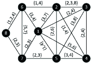
(a) Temporal graph $\mathcal{G}$

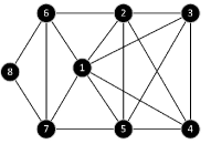
(b) Static graph $\bar{\mathcal{G}}$ of $\mathcal{G}$

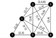
(c) Temporal subgraph $\mathcal{G}_{S_{1}}$

(d) Temporal subgraph $\mathcal{G}_{S_{2}}$

Figure 1. Temporal (sub)graph and static subgraph

Definition 1 (Temporal Triangle).

In a temporal graph $\mathcal{G}=(V,\mathcal{E},\mathcal{T})$, given three temporal edges $e_{1}(u,v,t_{1})$, $e_{2}(u,w,t_{2})$, $e_{3}(v,w,t_{3})\in\mathcal{E}$, if their static edges $\bar{e}_{1}(u,v)$, $\bar{e}_{2}(u,w)$, $\bar{e}_{3}(v,w)$ can form a triangle $\bar{\triangle}_{uvw}$, then we say $\triangle_{e_{1}e_{2}e_{3}}$ is a temporal triangle.

Similarly, the function $\odot$ converts a temporal triangle into its static counterpart, denoted as $\odot(\triangle)=\bar{\triangle}$. Let $\Delta(\triangle)=\max\{|t_{i}-t_{j}||1\leq i,j\leq 3\}$ denote the time span of $\triangle_{e_{1}e_{2}e_{3}}$ where $e_{1}$, $e_{2}$, and $e_{3}$ correspond to timestamps $t_{1}$, $t_{2}$, and $t_{3}$, respectively. Various time spans indicate different levels of interaction tightness, and individuals have varying criteria for assessing this tightness based on the time span. In a temporal graph, for a personalized parameter $\delta$ specified by users, the temporal property of a static triangle is characterized by the number of temporal triangles whose time span is no greater than $\delta$. This is expressed by the formula $N(\bar{\triangle},\delta)$=$|\{\triangle|\odot(\triangle)=\bar{\triangle},\Delta(\triangle)\leq\delta\}|$. Sometimes $N(\bar{\triangle},\delta)$ is abbreviated as $N(\bar{\triangle})$.

Definition 2 ($\delta$-Temporal Support).

Given an integer $\delta$, the $\delta$-temporal support of a static edge $\bar{e}(u,v)$ in the temporal graph $\mathcal{G}$ is denoted as $TSup_{\mathcal{G}}(\bar{e},\delta)$=$|\{\triangle_{e_{1}e_{2}e_{3}}|\exists e_{i}\in\triangle_{e_{1}e_{2}e_{3}}(i\in\{1,2,3\}),\odot(e_{i})=\bar{e},\Delta(\triangle_{e_{1}e_{2}e_{3}})\leq\delta\}|$. That is, it is the number of temporal triangles in the temporal graph $\mathcal{G}$ that involve a temporal edge $e$ satisfying $\odot(e)=\bar{e}$ and have a time span not exceeding $\delta$.

The temporal support of an edge can be rewritten as $TSup(\bar{e},\delta)=\sum_{\bar{e}\in\bar{\triangle}}N(\bar{\triangle},\delta)$. When the context is clear, we abbreviate $TSup_{\mathcal{G}}(\bar{e},\delta)$ to $TSup(\bar{e})$. It is straightforward to state the following proposition.

Proposition 1.

Given a temporal graph $\mathcal{G}$ and its subgraph $\mathcal{S}$, for any $\bar{e}\in\mathcal{S}$, we have $TSup_{\mathcal{G}}(\bar{e})\geq$ $TSup_{\mathcal{S}}(\bar{e})$.

Two triagnles $\triangle_{i}$ and $\triangle_{i+1}$ are considered connected if they share at least one common edge or vertex. Formally, this is expressed as $\triangle_{i}\cap\triangle_{i+1}\neq\emptyset$. Based on this definition, we define higher-order connectivity as follows:

Definition 3 (Higher-order Connectivity).

Given a parameter $\delta$, two triangles $\triangle_{1},\triangle_{n}$ are considered to be higher-order connected if the following two conditions are satisfied: (1) $\triangle_{1}$ and $\triangle_{n}$ can be connected by a sequence of triangles $\triangle_{1}$, …, $\triangle_{i}$, …, $\triangle_{n}$, where $n\geq 2$ and each pair of consecutive triangles $\triangle_{i}$ and $\triangle_{i+1}$ in this sequence must satisfy $\triangle_{i}\cap\triangle_{i+1}\neq\emptyset$. (2) $\forall 1\leq i\leq n$, $N(\bar{\triangle_{i}})\neq 0$.

Definition 4 ($(k,\delta)$-truss).

Given a temporal graph $\mathcal{G}$ and integers $\delta$ and $k$, a temporal subgraph $\mathcal{S}$ is called a $(k,\delta)$-truss if it satisfies the following conditions: (1) Cohesive: for every edge $\bar{e}\in\mathcal{S}$, $TSup_{\mathcal{S}}(\bar{e},\delta)\geq k$. (2) Connective: for every pair of edges $\bar{e}_{1},\bar{e}_{2}\in{\mathcal{S}}$, there exist triangles $\triangle_{x}$ and $\triangle_{y}$ such that $\bar{e}_{1}\in\triangle_{x},\bar{e}_{2}\in\triangle_{y}$, and $\triangle_{x}=\triangle_{y}$ or $\triangle_{x}$ and $\triangle_{y}$ are higher-order connected. (3) Maximal subgraph: there does not exist a subgraph $\mathcal{S}^{\prime}\subset\mathcal{G}$ such that $\mathcal{S}\subset{\mathcal{S}^{\prime}}$ and $\mathcal{S}^{\prime}$ satisfies condition (1) and (2).

Conceptually, a $(k,\delta)$-truss not only remains the cohesiveness of k-truss model, but also captures the tightness of time. Specifically, condition (1) ensures that the subgraph is densely connected under the structural constraints of the truss model, while the restriction $\delta$ on temporal triangles guarantees that the nodes are tightly connected. Condition (2) further enhances this by ensuring that all edges in $(k,\delta)$-truss are strongly connected through a series of powerful and stable triangles. Generally, a larger $k$ indicates that edges are connected through tighter temporal triangles, resulting in greater structural density and temporal compactness. Such communities are more desirable to users. Nevertheless, choosing an appropriate parameter $k$ is challenging. Small $k$ values may yield a large number of solutions, while large $k$ values might result in no matching communities. However, $k$ is closely related to the user-specified $\delta$, which helps in finding the maximal-$\delta$-truss with the maximal $k^{*}$.

Definition 5 (Maximal-$\delta$-truss, MDT).

Given a temporal graph $\mathcal{G}$ and an integer $\delta$, a temporal subgraph $\mathcal{S}$ is a maximal-$\delta$-truss of $\mathcal{G}$ if $\mathcal{S}$ is a $(k,\delta)$-truss such that $k$ is maximal, i.e. there is no other $(k^{\prime},\delta)$-truss with $k^{\prime}>k$.

Example 2.

Figure1(c) is an $(8,3)$-truss of Figure1(a), where each edge participates in at least eight temporal triangles with $\Delta(\triangle)\leq 3$. Figure1(d) is a $(12,3)$-truss. Since no other $(k,3)$-truss exists for $k>12$, Figure1(d) is the maximal-$\delta$-truss.

Users are typically more interested in communities that include the target nodes. So we aim to mine a MDT for a given query node.

Problem 1 (Maximal-$\delta$-truss mining).

For a temporal graph $\mathcal{G}$, a query node $q$, and an integer $\delta$, our objective is to find a maximal-$\delta$-truss containing $q$. This is denoted as q-MDT.

Theoretical challenges. Maximal-$\delta$-truss extends the properties of $k$-truss while maintaining the elegant properties of $k$-truss, such as $(k,\delta)$-truss $\subseteq(k-1,\delta)$-truss. Based on the idea from decompose (Huang et al., 2014), a naive global search method (GS) for the q-MDT problem is to iteratively remove the edges with the lowest temporal support. Specifically, we need to ascertain the temporal support of all edges to guide the selection process for edge deletion. According to Definition 1, a temporal triangle is a closed sequence of three temporal edges. Therefore, for a triangle $\bar{\triangle}_{uvw}=\{\bar{e}_{1}(u,v),\bar{e}_{2}(u,w),\bar{e}_{3}(v,w)\}$, we can count the number of the temporal triangle $\triangle_{e_{1}e_{2}e_{3}}$ with $\Delta(\triangle_{e_{1}e_{2}e_{3}})\leq\delta$ by checking the time span for all permutations of the temporal edges sequence. Then we compute $N(\triangle,\delta)$ for all triangles and accumulate $N(\triangle)$ to determine the temporal support for edges. Subsequently, we iteratively delete the edge $\bar{e}$ with the lowest temporal support and update the temporal support for edges sharing a triangle with $\bar{e}$. This continues until only one edge induced by $q$ remains, and then decompose returns the maximal temporal subgraph $\mathcal{S}$ with the lowest temporal support and maximal $k^{*}$. Finally, GS selects the connected components of $\mathcal{S}$ containing the query node $q$ by checking the connectivity of edges induced by $q$. This yields the final solution to our problem.

GS is not efficient since it needs to compute the temporal support for all edges in $\mathcal{G}$ and then greedily deletes the edges. Some edges may not meet the given temporal support and are irrelevant to the solution. For example, edges not connected to those induced by $q$ through a sequence of static triangles (against condition (1) in Definition 3) are not part of the solution, but GS still computes their temporal support. In addition, it is time consuming for GS as it begins its search from the entire graph. To address these inefficientcies, we propose a local search strategy in Section 3.

3. Local Search Strategy of q-MDT

One straightforward way to calculate the temporal support is to count the valid permutations of temporal edges. However, it is costly since there exist a large number of unnecessary operations. Here, we first calculate the temporal support by extracting edge timestamps and applying a sliding window technique. Subsequently, we locally explore the expanded temporal subgraph around the query node $q$ to find the solution of q-MDT.

3.1. Sliding Windows for Temporal Support

Computing $N(\triangle,\delta)$ by listing permutations of all temporal edges is expensive and unnecessary. However, if the time span of two temporal edges $e_{1}(u,v,t_{1}),e_{2}(u,w,t_{2})$ exceeds $\delta$, then any permutations that contain these two edges definitely cannot contribute to the temporal support. Inspired by this, we propose a new strategy using sliding windows to count the $\delta$-temporal triangles, as illustrated in Figure2.

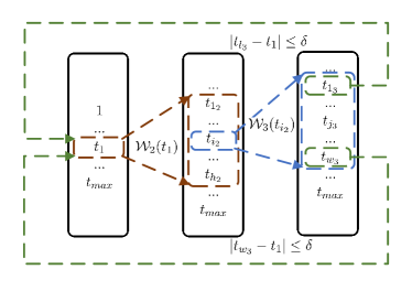
Figure 2. Sliding window for counting $N(\triangle,\delta)$

For a static triangle $\triangle=\{\bar{e}_{1},\bar{e}_{2},\bar{e}_{3}\}$, three sliding windows, each corresponding to one of the static edges, are used to count the number of temporal triangles that satisfy $\Delta(\tilde{\triangle})\leq\delta$. We first extract three timestamp lists $T(u,v)$, $T(u,w)$, $T(v,w)$ for edges in $\triangle_{uvw}$. Here, each list $T(x,y)$ contains the timestamps of all temporal edges in $\mathcal{G}=(V,\mathcal{E},\mathcal{T})$ corresponding to the static edge $(x,y)$, i.e., $T(x,y)=\{t|e(x,y,t)\in\mathcal{E}\}$. Specifically, we sort these lists in ascending order by their size and name them as $T_{1}$, $T_{2}$, $T_{3}$ respectively, such that $|T_{1}|\leq|T_{2}|\leq|T_{3}|$. For each timestamp $t_{1}$ in $T_{1}$, the algorithm maintains a window $\mathcal{W}_{2}(t_{1})={t_{1_{2}},...,t_{i_{2}},...,t_{h_{2}}}$ consisting of timestamps from $T_{2}$, such that every $t_{i_{2}}\in\mathcal{W}_{2}(t_{1})$ satisfies $|t_{1}-t_{i_{2}}|\leq{\delta}$. Similarly, $\forall t_{i_{2}}\in\mathcal{W}_{2}$, the algorithm records the window $\mathcal{W}_{3}(t_{i_{2}})=\{t_{1_{3}},...,t_{j_{3}},...,t_{w_{3}}\}$ for $T_{3}$, where $|t_{i_{2}}-t_{j_{3}}|\leq\delta$ and $|t_{1}-t_{j_{3}}|\leq\delta$ for $\forall t_{j_{3}}\in\mathcal{W}_{3}(t_{i_{2}})$.

Using sliding windows, we avoid the need to compute over the full $|T_{1}|\times|T_{2}|\times|T_{3}|$ space. Instead, for each timestamp $t_{1}$ in $T_{1}$, the number of temporal triangles with a time span not greater than $\delta$ is given by $\sum_{\begin{subarray}{c}t_{i_{2}}\in\mathcal{W}_{2}(t_{1})\end{subarray}}|\mathcal{W}_{3}(t_{i_{2}})|$. Therefore, we can quickly obtain the number of temporal triangles in $\mathcal{G}$ induced by $\triangle_{uvw}$. By accumulating $N(\triangle,\delta)$ for each triangle containing the edge $\bar{e}$, we can get the temporal support for $\bar{e}$.

3.2. Local Exploration for Candidate Subgraph

Condition (2) in Definition 4 requires that all edges in a $(k,\delta)$-truss must be connected, thus according to Definition 3, all edges must be connected by a series of triangles where $N(\triangle,\delta)\neq 0$. Consequently, if an edge cannot be connected to any edge induced by $q$ through a set of triangles, or if these triangles cannot induce a temporal triangle with a time span no greater than $\delta$, then these edges must not appear in q-MDT. Inspired by this, we locally explore the candidate temporal subgraph containing the q-MDT to avoid processing irrelevant edges.

Suppose $\mathcal{S^{*}}$ is a q-MDT, denoted as $(k^{*},\delta)$-truss. For each edge $\bar{e}\in\mathcal{S^{*}}$, we have $TSup_{\mathcal{S^{*}}}(\bar{e})\geq{k^{*}}$. If an edge $\bar{e}_{0}$ with $TSup_{\mathcal{G}}(\bar{e}_{0})<{k^{*}}$, it cannot appear in a q-MDT according to Proposition 1. Consequently, searching for a q-MDT in $\mathcal{G}$ is equivalent to searching it in the temporal subgraph $\mathcal{H}$, where each edge $\bar{e}$ satisfies $TSup_{\mathcal{G}}(\bar{e})\geq{k^{*}}$. Since $k^{*}$ is unknown, a naive approach is to calculate the temporal support for all edges induced by $q$ and choose the smallest value $k_{l}$ as the threshold to extract the subgraph where $TSup_{\mathcal{G}}(\bar{e})\geq k_{l}$. However, $k_{l}$ is usually small, sometimes even 0, leading to an overly large subgraph and high computational overhead.

We leverage the upper bound of $k^{*}$ and design a local search algorithm (LS) that performs a binary search on the temporal graph to get the expanded temporal subgraph. The key idea of LS is to find a small expanded temporal subgraph that contains the query node q, and then explore the exact solution in this subgraph. Given parameters $\delta$ and the original $k$, LS adopts a "compute-while-expanding" strategy to derive the expanded temporal subgraph $\mathcal{H}$. Initially, an edge $\bar{e}(q,v)$ induced by $q$ is selected. We then check if $TSup_{\mathcal{G}}(\bar{e}(q,v))\geq{k}$, where $k$ is an adjustable threshold. If the condition is satisfied, $\bar{e}(q,v)$ is considered as the first "expandable" edge. For each "expandable" edge $\bar{e}$, it computes the temporal support of the edges that are in the same triangle with $\bar{e}$, and picks up the new "expandable" edges for iterative expansion. The expanded temporal subgraph is obtained by iteratively expanding from the "expandable" edges $\bar{e}(q,v)$.

Proposition 2.

If an exact solution cannot be found in $\mathcal{H}$ constructed with threshold $k$, the subsequent threshold $k^{\prime}$ for the next round must be smaller than $k$, i.e. $k^{\prime}<k$.

Proposition 3.

For two temporal subgraphs $\mathcal{H}_{1}$ and $\mathcal{H}_{2}$ expanded with thresholds $k_{1}$ and $k_{2}$ respectively, if $k_{1}\leq{k_{2}}$, then $\mathcal{H}_{2}\subseteq{\mathcal{H}}_{1}$.

LS computes the temporal support of an edge only when it is accessed, thereby avoiding unnecessary computations and explorations of infeasible edges. For each expansion, the algorithm iteratively adjusts the threshold $k$ for temporal support and adds the edges whose temporal support is not less than $k$ to the expanded subgraph $\mathcal{H}$. This ensures that the expanded subgraph is neither too large nor too small. When computing the temporal support for an edge, if its current value is no less than $k$ then we can immediately stop access of the triangles it participates in. So both "compute-while-expanding" and "early stop" strategies improve the performance of exploration.

For the detailed algorithm description and pseudocode, please refer to Appendix B. Additionally, we provide an example in Appendix C.1 and analyze its complexity in Appendix D.2.

4. Fast q-MDT Search with Temporal Trussness

Compared with the baseline algorithm GS, the local exploration strategy shows better performance. LS still incurs some unnecessary visits because it needs to search some candidate subgraphs before the target communities are found. Moreover, the search space of the local method is related to the query node and the parameter $\delta$. So, it accesses a much larger search space when the graph is large or the parameter is big. In the cases, it generally leads to longer response time. One reason is that $LS$ method does not know where the possible q-MDTs are. If we know in advance the maximum value of $k$ (i.e. temporal trussness) in which each edge can participate in the $(k,\delta)$-truss, then we can search the highly possible target subgraphs instead of full search of the expanded subgrphs. By this way, we can prune much search space. Moreover, many queries may share the same parameter $\delta$. Especially it is true when the timespan of a graph is not large. Due to the above reasons, we propose a method using the temporal trussness to efficiently find solutions for q-MDT query.

4.1. Temporal Trussness (TT)

Each edge may appear in multiple triangles. However, A subgraph has several edges which have different values of $\delta$-temporal support. Here, we first define the temporal trussness of a subgraph, then define the temporal trussness of an edge.

Definition 6 (Temporal Trussness).

Given an integer $\delta$, the temporal trussness of a temporal subgraph $\mathcal{H}$ is the minimum temporal support of the edges in it, i.e. $\tau(\mathcal{S},\delta)=\min\{TSup_{\mathcal{S}}(\bar{e})|\bar{e}\in{{\mathcal{S}}}\}$. The temporal trussness of $\bar{e}\in{\mathcal{G}}$ is the maximal trussness of the temporal subgraphs that $\bar{e}$ participates in, where $\tau_{\mathcal{G}}(\bar{e},\delta)=\max\{\tau(\mathcal{S},\delta)|\bar{e}\in{\mathcal{S}},\mathcal{S}\subset{\mathcal{G}}\}$.

When it does not cause confusion, we abbreviate $\tau(\mathcal{S},\delta)$ and $\tau_{\mathcal{G}}(\bar{e},\delta)$ as $\tau(\mathcal{S})$ and $\tau(\bar{e})$, respectively.

If we want to know the temporal trussness of an edge, we first need to compute the $N(\triangle)$ of each triangle containing the edge so that we can get its temporal support and thus the temporal trussness. Suppose there are $|\triangle_{\mathcal{G}}|$ triangles in $\mathcal{G}$, we need $|\triangle_{\mathcal{G}}|\times t_{max}\times\delta^{2}$ to get $N(\triangle)$ of all triangles, so this method takes $|\triangle_{\mathcal{G}}|\times(t_{max})^{2}\times\delta^{2}$ to compute the temporal support for the edges in $\mathcal{G}$ under different $\delta$. It is very expensive if the temporal graph is large and spans a large time interval. Fortunately, although this way is a bit unsatisfactory, it still provides us with a new idea. When we set $\delta=t_{max}$ to compute the corresponding temporal support, as all temporal edges span no greater than $t_{max}$, so all the triangles in $\mathcal{G}$ satisfy that $N(\triangle)>0$ and all the temporal triangles in $\mathcal{G}$ satisfy that $\Delta(\tilde{\triangle})\leq t_{max}$. For each triangle $\triangle$ $\subset$ $\mathcal{G}$, $N(\triangle)$ is the number of the permutations of the temporal edges that lay on the edge in $\triangle$. Inspired on this observing, before introducing a novel algorithm to calculate the temporal support, we import a novel definition called $\delta$-slice which is a set of subgraphs whose time span is $\delta$.

Definition 7 ($\delta$-slice).

For a temporal graph $\mathcal{G}$ and an integer $\delta$, a $\delta$-slice is a sequence of temporal subgraphs of $\mathcal{G}$ in which the time span of each subgraph is $\delta$, denoted as $\mathcal{G}^{\delta}$=$\{\mathcal{G}_{[1,\delta+1]}$, $\mathcal{G}_{[2,\delta+2]}$, …, $\mathcal{G}_{[t_{max}-\delta,t_{max}]}\}$.

The range of $\delta$ is [$0$, $t_{max}$]. We shorten $\mathcal{G}_{[i,i+\delta]}$ to $\mathcal{G}_{i}^{\delta}$. When no misunderstanding occurs, $\mathcal{G}_{i}^{\delta}$ is further abbreviated to $\mathcal{G}_{i}$. Since the temporal graph can be decomposed into a list of temporal subgraphs, each of which starts at a specific timestamp and spans a specific interval $\delta$, we need to compute the temporal trussness of each temporal subgraph in the list. Computing the temporal trussness of all edges is time-consuming if a temporal graph has a large time span. In the following, we will discuss how to speed up the computation.

For each $\mathcal{G}_{j}$ in $\delta$-slice, it is easy to know the number of temporal triangles $N_{\mathcal{G}_{j}}(\triangle_{uvw})$=$|T_{\mathcal{G}_{j}}(u,v)|\times$ $|T_{\mathcal{G}_{j}}(u,w)|\times|T_{\mathcal{G}_{j}}(v,w)|$, where $T_{\mathcal{G}_{j}}(u,v)$ is the list of timestamps in edge $\bar{e}(u,v)$. By Definition 2, we get the following propositions and prove them in Appendix D.1.

Proposition 4.

Let $\mathcal{G}^{\delta}$ be a $\delta$-slice of $\mathcal{G}$. For a triangle $\triangle\subseteq\mathcal{G}$, its corresponding $N_{\mathcal{G}_{[i,i+\delta+1]}}(\triangle,\delta)$= $N_{\mathcal{G}_{i}^{\delta}}(\triangle,\delta)$+$N_{\mathcal{G}_{i+1}^{\delta}}(\triangle,\delta)$-$N_{\mathcal{G}_{i+1}^{\delta-1}}(\triangle,\delta-1)$.

Proposition 5.

Given a temporal graph $\mathcal{G}$ and an integer $\delta$, for a triangle $\triangle\subseteq\mathcal{G}$, its $N_{\mathcal{G}}(\triangle,\delta)=N_{\mathcal{G}}(\triangle,\delta-1)+\sum_{i=1}^{t_{max}-\delta}(\Phi_{N_{\mathcal{G}_{i}^{\delta}}(\triangle,\delta)}-\Phi_{N_{\mathcal{G}_{i+1}^{\delta-1}}(\triangle,\delta-1)})$, where $\Phi_{N_{\mathcal{G}_{i}^{\delta}}(\triangle,\delta)}=N_{\mathcal{G}_{i}^{\delta}}(\triangle,\delta)-N_{\mathcal{G}_{i}^{\delta-1}}(\triangle,\delta-1)$.

Proposition 6.

Given a temporal graph $\mathcal{G}$, an integer $\delta$ and the corresponding $\delta$-slice, $(\delta-1)$-slice, the temporal support of an edge $\bar{e}\in\mathcal{G}$ is given by: $TSup_{\mathcal{G}}(\bar{e},\delta)=TSup_{\mathcal{G}}(\bar{e},\delta-1)+\sum_{j=1}^{n}\sum_{i=1}^{t_{max}-\delta}(\Phi_{N_{\mathcal{G}_{i}^{\delta}}(\triangle_{j},\delta)}-\Phi_{N_{\mathcal{G}_{i+1}^{\delta-1}}(\triangle_{j},\delta-1)})$, where $\bar{e}\in\triangle_{j}$.

4.2. Bottom-up Incremental Computing

The temporal support of any edge under $\delta>t_{max}$ is same as that under $\delta=t_{max}$, since the time span of any two different temporal edges in $\mathcal{G}$ is not larger than $t_{max}$. So, based on previous propositions, we proposed the bottom-up algorithm (Algorithm 1) to compute the temporal support to obtain the trussness of the edges under different $\delta$. In the algorithm, we increase $\delta$ from $0$ to $t_{max}$ and incrementally compute temporal support and trussness. The algorithm includes two stages (Figure3). The trussness of each edge $\bar{e}\in\mathcal{G}$ will be saved in a list of pairs $(\delta,\tau(\bar{e}))$, such as $\{(0,\tau_{0}),...,(i,\tau_{i}),...,(t_{max},\tau_{t_{max}})\}$. Since it is a list of edge temporal trussness, we named it as TT-index.

Algorithm 1 Bottom-up Computing of Temporal Trussness

Input: A temporal graph $\mathcal{G}$

Output: The TT-index for $\mathcal{G}$

1:Initial $\Phi[\triangle]=0$;

2:for $\delta$ $\leftarrow{0}$ upto $t_{max}$ do

3:     CountAllTSup($\mathcal{G},\mathcal{H},\delta,\Phi$);

4:     decompose($\mathcal{G}$,$\delta$,TT);

5:return TT;

Algorithm 2 CountAllTSup

Input: $\mathcal{G}$, $\delta$, $\mathcal{G}^{\delta}$, $\mathcal{G}^{\delta-1}$ and $\Phi$

Output: $\forall\triangle\subseteq\mathcal{G},N_{\mathcal{G}}(\triangle,\delta),\forall\bar{e}\in\mathcal{G},TSup_{\mathcal{G}}(\bar{e},\delta)$

1:Let $\mathcal{P}[\triangle]$ record the value of $\Phi_{N_{\mathcal{G}_{1}^{\delta}}(\triangle,\delta)}$ ;

2:Initial $\Phi^{\prime}=\Phi$;

3:for $t\leftarrow{1}$ upto $t_{max}-\delta$ do

4:     for $\bar{e}(u,v)\in\mathcal{G}_{[t+\delta,t+\delta]}$ do

5:         $\mathcal{G}_{t}^{\delta}=\mathcal{G}_{t}^{\delta-1}\cup e(u,v,t)$;      

6:     for $\bar{e}(u,v)$ in $\mathcal{G}_{[t+\delta,t+\delta]}$ do

7:         for $w$ in $\mathcal{D}_{\mathcal{G}_{t}^{\delta}}(u)\cap\mathcal{D}_{\mathcal{G}_{t}^{\delta}}(v)$ do

8:              $s=|T_{\mathcal{G}_{t}^{\delta}}(u,v)|*|T_{\mathcal{G}_{t}^{\delta}}(u,w)|*|T_{\mathcal{G}_{t}^{\delta}}(v,w)|$;

9:              $\Phi[\triangle_{uvw}]+=s-N_{\mathcal{G}_{t}^{\delta-1}}(\triangle_{uvw})$;

10:              if $t=1$ then

11:                  $\mathcal{P}[\triangle_{uvw}]=\Phi[\triangle_{uvw}]$;               

12:              $N_{\mathcal{G}_{t}^{\delta}}(\triangle_{uvw})=s$;               

13:for $\triangle_{uvw}$ in $\Phi$ do

14:     if $\Phi[\triangle_{uvw}]=0$ then

15:         continue;      

16:     if TT[$\triangle_{uvw}$] has not been recorded then

17:         $\textit{TT}[\triangle_{uvw}]\leftarrow{\delta}$      

18:     $\varphi=\Phi[\triangle_{uvw}]-\Phi^{\prime}[\triangle_{uvw}]$;

19:     $N_{\mathcal{G}}(\triangle_{uvw},\delta)\leftarrow{N_{\mathcal{G}}(\triangle_{uvw},\delta-1)+\varphi}$;

20:     $TSup_{\mathcal{G}}(\bar{e}(u,v),\delta)\leftarrow{TSup_{\mathcal{G}}(\bar{e}(u,v),\delta-1)+\varphi}$;

21:     $TSup_{\mathcal{G}}(\bar{e}(u,w),\delta)\leftarrow{TSup_{\mathcal{G}}(\bar{e}(u,w),\delta-1)+\varphi}$;

22:     $TSup_{\mathcal{G}}(\bar{e}(v,w),\delta)\leftarrow{TSup_{\mathcal{G}}(\bar{e}(v,w),\delta-1)+\varphi}$;

23:     $\Phi[\triangle_{uvw}]=\Phi[\triangle_{uvw}]-\mathcal{P}[\triangle_{uvw}]$;

In the first stage (Left part of Figure3, Algorithm 2), the algorithm iteratively generates $\delta$-slice of $\mathcal{G}$ and computes the number of temporal triangles in each interval. Specifically, when the algorithm increases $\delta$ by 1, temporal subgraph $\mathcal{G}_{i}^{\delta-1}$ in $(\delta-1)$-slice will be expanded to include the edges in snapshot $\mathcal{G}_{[i+\delta,i+\delta]}$ (Line 4-5). So, the temporal subgraph $\mathcal{G}_{i}^{\delta}$ can be derived from $\mathcal{G}_{i}^{\delta-1}$. The added edges will induce new triangles and change $N(\triangle)$ of the existing triangles, as well as the $TSup(\bar{e})$ of the edges in these triangles. The algorithm computes $N_{\mathcal{G}_{i}^{\delta}}(\triangle,\delta)$ for all triangles and then updates $\Phi$ based on the increment (Lines 8-9). The increment of $N(\triangle)$ for triangles in $\mathcal{G}_{1}^{\delta}$ (denoted as $\mathcal{P}$) is saved for the next iteration (Lines 10-11). The algorithm then traverses and updates these triangles and their relevant edges. Specifically, for a triangle $\triangle$, if the increment $\Phi[\triangle]=0$, this indicates that $N(\triangle,\delta)$ remains unchanged, i.e., $N(\triangle,\delta)=N(\triangle,\delta-1)$, and thus the edges within it are unaffected (Lines 14-15). Otherwise, the algorithm updates $N(\triangle,\delta)$ for the triangles and adjusts the temporal support of the edges within those triangles (Lines 18-22). Additionally, if a triangle has an increment, it must be true that $N(\triangle)>0$. Consequently, Algorithm 2 updates the TT-index (Lines 16-17) to record the minimum value of $\delta$ at which $N(\triangle,\delta)>0$, allowing for quick determination of edge connectivity. Finally, the algorithm updates the increment to facilitate the next iteration (Line 23).

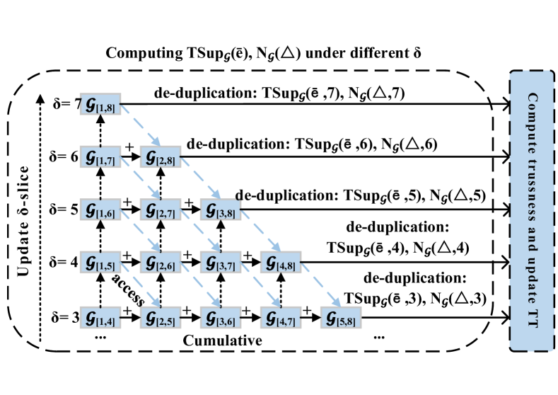
Figure 3. The construction framework of the TT-index

In the next stage (Right part of Figure3), the adapted decomposition algorithm decompose (Huang et al., 2014) computes the trussness and continually updates the TT-index (Line 4 in Algorithm 1) until all reasonable value of $\delta$ had been processed. The temporal trussness of each edge for $\delta$ is at least as large as its temporal trussness for $\delta-1$, namely $\tau(\bar{e},\delta)\geq{\tau(\bar{e},\delta-1)}$. In fact, the temporal trussness of an edge may be the same for adjacent $\delta$ values. To conserve storage, only the changed pairs are saved. Specifically, a pair $(\delta_{i},\tau_{i})$ for an edge is stored in TT if and only if there are no other pairs $(\delta_{j},\tau_{j})$ satisfy $\delta_{j}<\delta_{i}$ and $\tau_{i}\leq\tau_{j}$.

4.3. Query Processing

As previously mentioned, for a specific $\delta$, the temporal trussness of an edge $\tau(\bar{e})$ is the maximal $k$ that participates in a $(\tau(\bar{e}),\delta)$-truss. For a query node $q$, identifying the $k^{*}$ of the q-MDT becomes straightforward, as it is equal to the smallest trussness of the edges induced by $q$. TTS algorithm (Algorithm 3) outlines the strategy of using TT-index to search for q-MDT. The algorithm first queries the trussness of all edges induced by $q$ from TT and marks the max trussness as $k^{*}$ (Lines 2-8). Specifically, for a given $\delta$, to identify the trussness of edges in $\mathcal{G}$, the algorithm calls Procedure $FindIndex$ to access TT and returns a pair $(d,\tau)$, where $d\leq\delta$ and $d$ is maximal. During this process, a deque $Q$ is maintained to store the edges induced by $q$. If an edge has a trussness with $\tau<k^{*}$, it is excluded from the q-MDT, and the algorithm marks it as visited to avoid repeat checks (Lines 4-5). Otherwise, the algorithm continues to remove edges from $Q$ until no edge in $Q$ has a trussness less than $k^{*}$ (Lines 6-7). Then, the algorithm pushes the current edge into $Q$ and update $k^{*}$ accordingly (Line 8).

Algorithm 3 Searching q-MDT using Temporal Trussness (TTS)

Input: $\mathcal{G}$, $q$, $\delta$, and TT
  Output: The q-MDT solution

1:Initial $vis=\emptyset$, $Q=\emptyset$, $k^{*}=0$, $i=0$;

2:for $u$ in $\mathcal{D}_{\mathcal{G}}(q)$ do

3:     $(k,d)=FindIndex(\mathcal{G},\bar{e}(q,u),\delta)$;

4:     if $k<k^{*}$ then

5:         $vis\leftarrow{vis}\cup{\bar{e}(q,u)}$; continue;      

6:     while $!Q.empty()$ and $\tau(Q.front())<k$ do

7:         $Q.pop\_front()$; $vis\leftarrow{vis}\cup{\bar{e}(q,u)}$;      

8:     $Q.push\_front(\bar{e})$; $k^{*}=max(k^{*},k)$;

9:while $!Q.empty()$ do

10:     $\bar{e}=Q.pop\_front();Q_{s}=\emptyset$ 

11:     if $\bar{e}(q,u)$ is in $vis$ then

12:         continue;      

13:     $\mathcal{S}_{i++}=\emptyset$; $Q_{s}.push(\bar{e}(u,v))$;

14:     while $!Q_{s}.empty()$ do

15:         $\bar{e}(u,v)=Q_{s}.pop();$ $\mathcal{S}_{i}.add(\{e(u,v,t)\in{\mathcal{G}}\})$;

16:         for $w\in\mathcal{D}(u)\cap\mathcal{D}(v)$ do

17:              if $TT[\triangle_{uvw}]>\delta$ then

18:                  continue;

19:                  if $FindIndex(\bar{e}(u,w),\delta).second\geq k^{*}$ and $FindIndex(\bar{e}(v,w),\delta).second\geq k^{*}$ then

20:                       if $\bar{e}_{1}(u,w)$ is not in $vis$ then

21:                           $Q_{s}.push(\bar{e}_{1})$; $vis\leftarrow{vis\cup{\bar{e}_{1}}}$;                        

22:                       if $\bar{e}_{2}(v,w)$ is not in $vis$ then

23:                           $Q_{s}.push(\bar{e}_{2})$; $vis\leftarrow{vis\cup{\bar{e}_{2}}}$;                                                                      

24:return ${\mathcal{S}_{1},\mathcal{S}_{2},...,\mathcal{S}_{i}}$;

After getting the value of $k^{*}$, the search process starts with the edges in $Q$ induced by $q$ whose trussness are no less than $k^{*}$. For each edge $\bar{e}(u,v)\in Q$, the algorithm accesses the edges that are in the same triangle with $\bar{e}(u,v)$. For the triangle $\triangle\in\{\triangle_{uvw}|\bar{e}(u,w),\bar{e}(v,w)\in\mathcal{G}\}$, to judge whether $\triangle$ can be a bridge to connect two edges, the algorithm only needs to access the TT-index to obtain $TT[\triangle]$ (the minimal $\delta$ makes it satisfy $N(\triangle)>0$), instead of recalculating the $N(\triangle,\delta)$ of it. In more details, $TT[\triangle]>\delta$ indicates that the triangle $\triangle$ cannot satisfy condition (2) in Definition 4 under the current $\delta$, so that we cannot find the connected edges through $\triangle$ (Lines 17-18). Otherwise, the algorithm continues to judge if the edges within this triangle are valid (Line 19). According to the Definition 5, if the trussness of both $bare(u,w)$ and $bar(v,w)$ is not less than $k^{*}$, this indicates that both edges can be contained in q-MDT. In this way, we may be able to search some other edges in the final solution through these edges. Therefore, Algorithm 3 pushes them into queue $Q_{s}$ and updates their states as visited (Lines 16-20). When $Q_{s}$ is empty, the current temporal subgraph $\mathcal{S}_{i}$ is a q-MDT. And when $Q$ is empty, all qualified q-MDTs have been found and the algorithm returns. An example is provided in Appendix C.2 to illustrate the query process.

5. Experimental Evaluation

We conducted experiments on nine real-world datasets and selected seven state-of-the-art models (MAPPR, k-truss, OL, PCore, DCCS, FirmCore, L-MEGA) as benchmarks to evaluate the efficiency, effectiveness, and scalability of the proposed methods. GS adopts the global strategy with a Sliding Window procedure for q-MDT search. LS and TTS are our optimized methods which search the q-MDT with local strategy and temporal trussness index (TT-index), respectively. We set $\delta$=8 unless specified otherwise. Further details about the experimental setup are provided in Appendix E.1.

5.1. Efficiency Evaluation

Exp-1: Storage and Construction Time for Building TT. Table 1 shows the storage requirements and construction time for TT. $\textit{TT}[\bar{e}]$ and $\textit{TT}[\triangle]$ are the storage of the temporal trussness for each edge and triangle, respectively. Regarding construction time, in all datasets, our algorithm builds the TT-index within one day for all datasets. It is usually necessary to sacrifice a certain amount of space to achieve this result. For example, $\textit{TT}[\triangle]$ requires up to about five times the storage of the raw temporal graphs (LS) in the $Thiers$ dataset. However, the storage does not increase in all datasets. The size of TT[$\triangle$] is even smaller than that of the input graph in the $Rmin$, $Twitter$ and $Facebook$ datasets. This discrepancy arises due to TT[$\triangle$]’s strong dependence on both the time span and the structure of the input graphs. A longer time span results in a greater number of $\triangle$ stored in TT[$\triangle$], consequently enlarging the storage requirements. For the same reasons, $\textit{TT}[\bar{e}]$ consumes between 0.25 to 98 times the space occupied by the original temporal graphs in LS. Theoretically, on the $Rmin$ dataset, $\textit{TT}[\bar{e}]$ would take up 5579 times more space than the original graph, but in practice it is only about 98 times. This demonstrate the effectiveness of our non-domain strategy.

Table 1. Storage (in MB) and Construction Time (in Sec.)

Dataset	LS	TTS
		$\textit{TT}[\bar{e}]$	$\textit{TT}[\triangle]$	Index Time
Rmin	0.854	83.3	0.237	43174
Primary	0.348	0.885	0.810	23
Lyon	2.81	4.11	12.42	1248
Thiers	3.98	16.1	20.9	5570
Twitter	6.69	1.7	1.17	19
Facebook	7.15	16.4	1.62	1407
Enron	10	50.5	10.11	5026
Lkml	4.04	51.4	14.22	3386
DBLP	191.82	210.38	404.21	53826

Table 2. The Running Time of Temporal Methods (ms). $*$ indicates the corresponding method cannot obtain results within two days.

Dataset	OL	PCore	DCCS	FirmCore	L-MEGA	GS	LS	TTS
Rmin	47.121	769.308	*	4112.281	2.420	0.577	0.469	0.003
Primary	69.515	11.463	4.094	0.959	16.0203	0.924	0.352	0.005
Lyon	1635.670	38524.712	19.335	3.587	787.731	50.560	48.514	0.831
Thiers	2077.790	10603.183	175.428	16.084	290.311	56.754	26.501	0.379
Twitter	353.517	66.362	8.323	26.036	*	7.887	0.444	0.056
Facebook	51.213	28967.205	3796.355	2413.352	*	4.435	0.206	0.018
Enron	267.906	153909.163	491.361	2073.825	*	27.515	4.489	0.283
Lkml	3130.130	159965.765	1638.877	44.882	*	79.022	16.547	0.839
DBLP	2435.710	185.330	5236.058	8080.973	*	446.099	339.240	40.660
AVG.RANK	6	7	5	4	8	3	2	1

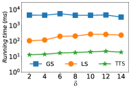
(a) Facebook (vary $\delta$)

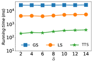
(b) Enron (vary $\delta$)

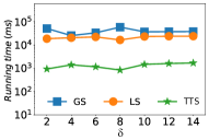
(c) Lkml (vary $\delta$)

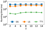
(d) DBLP (vary $\delta$)

Figure 4. Running Time of Different Methods with Varying $\delta$.

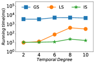
(a) Facebook (vary $d_{\mathcal{G}}(q)$)

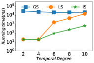
(b) Enron (vary $d_{\mathcal{G}}(q)$)

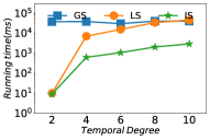
(c) Lkml (vary $d_{\mathcal{G}}(q)$)

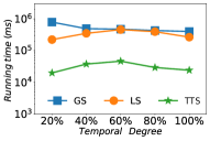
(d) DBLP (vary $d_{\mathcal{G}}(q)$)

Figure 5. Running Time with Varying Temporal Degree of Query Nodes.

Exp-2: The Running Time of Different Methods. Table 2 shows the running time of eight methods on nine datasets, where the last row displays the ranking based on the average rank. TTS and LS rank top and second, respectively. Especially, TTS takes less than one second on eight datasets and under a minute on $DBLP$. GS is slightly slower than LS due to its unnecessary calculations. FirmCore and DCCS are the fourth and fifth, respectively, because they spend much time finding the basic core model and integrating them as solutions. OL and PCore perform poorly since both require many iterations to return optimal results. L-MEGA returns the solutions on four small datasets within a reasonable time but fails to return a solution within two days for the other five datasets. This demonstrates that our optimal strategies are effective in practice.

Exp-3: Running Time of Different Methods with Varying $\delta$. In this experiment, we selected four datasets and three different search strategies to report the effect of parameter $\delta$ on the running time, as shown in Figure4. The search strategy GS always requires the longest time to return a solution across all datasets, highlighting the efficacy of the optimization strategies employed in LS. TTS has the best performance since it only executes a simple search strategy based on the TT-index, which minimizes redundant accesses. Compared to GS, TTS achieves a speedup of at least two orders of magnitude across most datasets, indicating its capability to efficiently handle a high volume of queries.

Exp-4: Running Time with Varying Temporal Degree of Query Nodes. We selected query nodes based on varying temporal degrees to analyze their impact on running time. For each dataset, nodes were sorted by ascending temporal degree and divided into five equally sized buckets. From each bucket, 100 nodes were randomly chosen as query seeds for searching the q-MDT using three methods. The results (see Fig. 5) indicate that GS is insensitive to the temporal degree of query nodes due to its nature as a global algorithm, which needs to search the entire input graph. In contrast, both LS and TTS show increased running times as the temporal degree of query nodes rises. One reason is that nodes with higher temporal degrees tend to participate in larger q-MDTs, necessitating longer search times. TTS particularly benefits in these scenarios compared to LS, as it focuses on searching a restricted set of nodes. Therefore, TTS is more practical, especially when users prioritize communities where initial nodes have extensive interactions with others.

Table 3. Effectiveness of Temporal Methods. $*$ denotes the corresponding model cannot be returned in two days.

		k-truss	MAPPR	OL	PCore	DCCS	FirmCore	L-MEGA	q-MDT
HTD	Rmin	0.00007	0.00089	0.00498	0.00176	*	0.00414	0.00021	0.01106
	Primary	0.00479	0.03768	0.13751	0.0461	0.15874	0.0221	0.0669	0.1609
	Lyon	0.02038	0.09283	0.14888	0.78574	0.09654	0.1	0.00021	0.1426
	Thiers	0.00925	0.04642	0.12805	0.09655	0.08434	0.04516	0.01963	0.13751
	Twitter	0.0008	0.001	0.34056	0.00341	0.11696	0.08879	*	0.36365
	Facebook	0.01016	0.00001	0.01508	0.15081	0.1	0.00001	*	0.07368
	Enron	0.00025	0.00685	0.01804	0.00241	0.00001	0.00418	*	0.14095
	Lkml	0.06299	0.18989	0.26226	0.13408	0.01125	0.16105	*	0.52042
	DBLP	0.39787	0.57478	0.6401	0.51182	0.22405	0.54407	*	0.80436
	AVG.RANK	7	5	2	3	4	6	8	1
HTC	Rmin	1	0.73225	0.90037	0.67877	*	0.67787	0.7211	0.57939
	Primary	0.79225	0.56849	0.97105	0.52811	0.80813	0.86898	0.54241	0.7802
	Lyon	1	0.83441	0.95451	0.90039	0.99767	0.97431	0.75084	0.91382
	Thiers	1	0.78531	0.75383	0.98391	0.9391	0.9966	0.68487	0.66646
	Twitter	0.74328	0.70028	0.96348	0.77779	0.92273	0.9314	*	0.65159
	Facebook	0.6932	0.676	0.69151	0.69329	0.25791	0	*	0.66891
	Enron	0.82007	0.68761	0.98123	0.96308	0.8645	0.89774	*	0.60762
	Lkml	0.99698	0.87261	0.99189	0.93365	0.90057	0.90263	*	0.81753
	DBLP	0.51533	0.66011	0.77391	0.81835	0.8868	0.03288	*	0.64509
	AVG.RANK	7	3	8	5	6	4	1	2

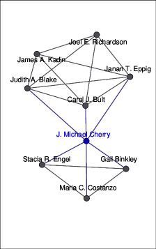
(a) PCore

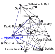
(b) OL

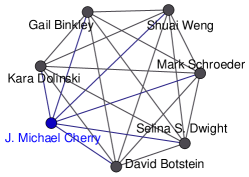
(c) Our model (q-MDT)

Figure 6. Case studies on DBLP. The blue vertex (i.e., J. Michael Cherry) is the query vertex.

5.2. Effectiveness Evaluation

Currently, there are no established metrics for assessing the attributes of higher-order temporal communities. Existing well-known metrics such as EDB (Edge Density Burstiness) (Lin et al., 2022a; Chu et al., 2019; Zhu et al., 2022) and TC (Temporal Conductance) (Zhang et al., 2022; Lin et al., 2022a; Zhu et al., 2022) focus on temporal edges and are therefore suitable for evaluating low-order temporal communities. To address this gap, we propose two new metrics, HTD and HTC, which incorporate temporal triangles instead of temporal edges. In HTD and HTC, temporal triangles must satisfy $\Delta(\triangle)\leq\delta^{*}$. Here, we let

(1) $$HTD=\sqrt[3]{\frac{|\{\triangle|\Delta(\triangle)\leq\delta^{*},\odot(\triangle)\subset\mathcal{G}_{S}\}|}{|S||S-1||S-2||T_{S}|^{3}}}$$

(2) $$HTC=\frac{|HTcut(S,V\backslash S)|}{min\{HTvol(S),HTvol(V\backslash S\}}$$

(3) $$HTcut(S,V\backslash S)=\{\triangle_{uvw}|\Delta(\triangle)\leq\delta^{*},\exists u,v,w\in S\}$$

(4) $$HTvol(S)=\{\triangle_{uvw}|u\in S,\Delta(\triangle)\leq\delta^{*}\}$$

To ensure fairness, we first compute the average gap of the temporal edges to estimate $\delta^{*}$ as proposed by Li et al. (Li et al., 2018). Subsequently, this estimate is utilized in the calculation of temporal triangles. This approach allows us to assess the density of higher-order temporal triangles effectively while preserving the integrity of experimental results. A higher value of HTD signifies a denser temporal community. HTC measures the degree distribution within the solution, where a smaller HTC indicates more intra-solution connections and fewer external ties.

Exp-5: Effectiveness of Temporal Models. For HTD metric, our model obtains the best grade on six datasets (Table 3). Following closely is OL, which defines bursting communities as clique-like subgraphs with higher triangle density. Other temporal models, such as PCore, DCCS, and FirmCore, show better performance than the static k-truss because the latter does not consider temporal information of subgraphs. In contrast, L-MEGA underperforms as it only optimizes the higher-order conductance at each timestamp. In terms of HTC metric, our model and L-MEGA exhibit similar performance on datasets where L-MEGA runs successfully. The reason is that L-MEGA optimizes its solutions based on triangle conductance (Fu et al., 2020), which is highly relevant with HTC. In contrast, MAPPR, which also utilizes triangle conductance to identify communities, performs less effectively than L-MEGA. This is because MAPPR is a completely static method, but L-MEGA uses the temporal information to optimize its solution. In general, PCore outperforms other core models such as DCCS and FirmCore due to its strong persistence correlation with $\delta^{*}$. It’s notable that the HTC of k-truss on datasets like $Rmin$, $Lyon$ and $Thiers$ reaches $1$, indicating that their solutions are indistinguishable with the other parts. This occurs because these datasets exhibit dense structures when temporal information is disregarded, and returned almost the entire graph. This experiment underscores our model’s capability to discover higher-quality communities compared to other models.

Exp-6: Case Study on DBLP. In this section, we present results for k-truss, PCore, OL, and q-MDT. Due to space limitations, we omit similar results obtained by other models. The community identified by k-truss includes over 1,000 authors spanning diverse research domains like computational biology, chemical reactions, and data mining. This community is too large to visualize effectively in a figure, which is why no visualization is provided. Notably, k-truss only captures the structural cohesiveness of temporal graphs but does not consider the temporal information. PCore returns a community with nine authors, divided into two groups connected by J. Michael Cherry (see Figure6(a)). The upper part consists of authors primarily affiliated with the Jackson Laboratory, whereas the lower group consists of individuals from Stanford University. Consequently, the community exhibits loose connections and lacks cohesion around J. Michael Cherry, resulting in a less dense structure. OL returns a community with 11 authors as shown in Fig.6(b). Compared with PCore, OL provides a more meaningful solution. However, it includes two authors, Catherine A. Ball and Midori A. Harris, who each collaborate with only one other author within this community. In fact, Catherine A. Ball shares research interests in Gene Expression Profiling and Bioinformatics with Gavin Sherlock, who frequently collaborates with J. Michael Cherry. Our model (q-MDT) identifies a community consisting of seven authors, all specializing in genetics as J. Michael Cherry (see Figure6(c)). They were colleagues of J. Michael Cherry at Stanford University from 1990 to 2013. David Botstein and J. Michael Cherry co-founded the Saccharomyces Genome Database, a significant international resource connecting genomic sequences with biological functions. This community formation is attributed to their shared research interests and enduring collaboration with J. Michael Cherry over the years. In conclusion, our model q-MDT can find more practical and meaningful communities in real-world scenarios.

Additionally, the detailed information about scalability experiments is available in AppendixE.2.

6. Conclusion

In this paper, we introduce a novel higher-order temporal community model called maximal-$\delta$-truss (MDT), in which all edges are connected by a sequence of triangles with well-defined temporal properties. The MDT model captures both the structural and temporal information of subgraphs through these temporal triangles within a constrained time span. To find a MDT around a specific query node $q$ (q-MDT), we propose a local strategy that combines an expanding algorithm to incrementally explore potential subgraphs, followed by searching q-MDT in the expanded temporal subgraph. Additionally, we develop the TT-index to expedite queries, facilitating efficient processing of large-scale graph queries. Empirical results on nine real-world networks, compared with seven competitors, demonstrate the efficiency, effectiveness, and scalability of our solutions.

Appendix A Related Work

Static Community Mining. Delving deeply into graphs to capture inside relationships among entities has attracted a great deal of researches, which propose multiple community models, including k-core (Cheng et al., 2011) (Li et al., 2015), clique (Pardalos and Xue, 1994)(Wu and Hao, 2015), and k-ECC (Li et al., 2017)(Chang et al., 2013). Subsequently, many researches, such as $k$-clique (Tsourakakis, 2015) and $\gamma$-quasi-clique (Yuan et al., 2018) extend the models in order to describe community more comprehensively. Goldberg (Goldberg, 1984) defined the densest subgraph which takes the average node degree as the metric to evaluate its structure characteristic. Andersen and Chellapilla (Andersen and Chellapilla, 2009) developed algorithms to find the densest subgraphs with two different size restriction. Han et al. (Han et al., 2016) proposed an association classification algorithm based on node centrality and the strength of structural relationships between nodes and associations. Hong et al. (Hong et al., 2022) proposed a model named GraphReformCD to find the strongly connected nodes in community. Gao et al. (Gao et al., 2020) proposed PCCD model to mine communities in sparse graphs. However, these studies focus on the lower-order community which is defined based on nodes and edges, ignoring the higher-order connectivity. Therefore, the higher-order model $k$-truss (Cohen, 2008; Huang et al., 2014) takes the triangles as basic blocks to build communities. Akbas and Zhao (Akbas and Zhao, 2017) designed an EquiTruss index to speed up the search for truss communities. Besides, Liu et al. (Liu et al., 2020) extended the truss model to directed graphs and developed a $D$-truss model. Yin et al. (Yin et al., 2017) proposed MAPPR model which combine motifs with classical approximate personalized PageRank. Unfortunately, these existing higher-order methods cannot be used directly in the temporal networks as they ignore the temporal information.

Temporal Community Mining. There are many researches extend the static models to temporal networks to capture both their structural and temporal information. For example, Li et al (Li et al., 2018) defined the persistent community in temporal networks based on $k$-core model (Cheng et al., 2011; Li et al., 2015). Zhu et al. (Zhu et al., 2018) and Hashemi et al. (Hashemi et al., 2022) search for the core-based dense subgraphs in discontinuous time layer. Yu et al (Yu et al., 2021) propose an index-based method with pruning strategies to speed up the search of historical $k$-cores. Similarly, Yang et al (Yang et al., 2016) and Lin et al (Lin et al., 2022b) combined the temporal information with the structure properties of clique to explore temporal quasi-cliques. Chu et al (Chu et al., 2019) and Rozenshtein et al (Rozenshtein et al., 2020) extended the basic concept of density to temporal networks, and proposed the corresponding algorithms to solve these NP-hard problems. Besides, Ma et al (Ma et al., 2017) proposed a series algorithms to solve the problem of finding heavy temporal subgraph in a special temporal networks where entity relationships keep fixed while the weight of edges change. Qin et al. (Qin et al., 2020) developed a novel model to explore the periodicity of the community in temporal networks. Zhang et al. (Zhang et al., 2022) adopted two different strategies, top-down and bottom-up, to search their significant community. Besides, Wang et al. (Wang et al., 2022) used HR2vec method to capture user behavior from individual users to communities and entire networks. Qin et al. (Qin et al., 2022) propose periodic community models in temporal networks, including $\sigma$-periodic $k$-core and $\sigma$ -periodic $k$-clique. Tang et al. (Tang et al., 2022) propose a ($\theta,k$)-core reliable community (CRC) model in the weighted dynamic networks. However, these explorations in temporal networks mainly focus on the low-order structure of communities. So, few studies have attempted to explore the higher-order properties of communities in temporal networks. Paranjape et al. (Paranjape et al., 2017) counted the higher-order temporal motifs to explore the structure and function of temporal networks. Wang et al. (Wang et al., 2020) provided an approximate temporal motif counting via random sampling. Porter et al. (Porter et al., 2022) also developed a fast and accurate model-based method for counting motifs in temporal networks. However these methods only count the number but not promote the community. L-MEGA (Fu et al., 2020) mines higher-order communities in time-evolving networks, starting with an query node and clustering the nodes with motif sub-structure. Unfortunately, capturing temporal information complicates the search for L-MEGA in massive temporal networks. Thus it is necessary to develop a novel model for finding higher-order communities.

Appendix B Pseudocode for Local Exploration Strategies

For clarity, we divide the local search algorithm (LS) into two parts: local exploration strategy for finding MDT (Algorithm 4) and expanding (Algorithm 5).

Algorithm 4 Local exploration strategy for finding MDT (LS)

Input: Temporal graph $\mathcal{G}$, integer $\delta$ and node $q$

Output: The q-MDT solution

1:$k_{l}=INT\_MAX,k_{h}=INT\_MIN$;

2:$k^{*}=0$, $\mathcal{S}=\emptyset$, $\mathcal{H}=\emptyset$, $Q_{1}=\emptyset$;

3:for $v$ in $\mathcal{D}(q)$ do

4:     compute $TSup_{\mathcal{G}}(\bar{e}(q,v))$ with Sliding Window;

5:     $k_{l}=min(k_{l},TSup(\bar{e}))$; $k_{h}=max(k_{h},TSup(\bar{e}))$;

6:while $k_{l}\leq{k_{h}}$ do

7:     $k_{m}=(k_{l}+k_{h})/2$;

8:     $\mathcal{B},Q_{1}$= Expanding$(\mathcal{G},\delta,Q_{1},k_{m},q)$;

9:     for $\bar{e}(u,v)\in\mathcal{B}$ do

10:         $\mathcal{H}=\mathcal{H}\cup\{e(u,v,t)|e(u,v,t)\in\mathcal{G}\}$;

11:         update $TSup_{\mathcal{H}}$ for related edges in $\mathcal{H}$;      

12:     $\mathcal{S}$, $k_{\mathcal{H}}^{*}$=decompose($\mathcal{H},q$);

13:     if $k_{\mathcal{H}}^{*}=0$ then

14:         $k_{h}=k_{m}$;      

15:     if $k_{\mathcal{H}}^{*}\neq 0$ and $k_{\mathcal{H}}^{*}<k_{m}$ then

16:         $k_{l}=k_{\mathcal{H}}^{*};k_{h}=k_{m}$;      

17:     if $k_{\mathcal{H}}^{*}\neq 0$ and $k_{\mathcal{H}}^{*}\geq k_{m}$ then

18:         check connective property from $q$ and return;      

Algorithm 4 begins by recording both the smallest $k_{l}$ and largest $k_{h}$ temporal support values (Line 5). It then selects $k_{m}=(k_{l}+k_{h})/2$ as the threshold and calls Algorithm 5 to extract an expanded subgraph $\mathcal{H}$ where all edges satisfy $TSup_{\mathcal{G}}(\bar{e})\geq k_{m}$ (Lines 7-11). After that, the algorithm calls decompose to get the current $k_{\mathcal{H}}^{*}$ of the q-MDT in $\mathcal{H}$ (Line 12). Note that $k_{\mathcal{H}}^{*}$ can indicate what Algorithm 4 will do next:

Case 1 (Lines 13-14): If $k_{\mathcal{H}}^{*}=0$, the threshold $k_{m}$ is too strict, causing the expanded temporal subgraph may be much smaller than the exact solution. The algorithm updates $k_{h}=k_{m}$ and generates a new expansion.

Case 2 (Lines 15-16): If $0<k_{\mathcal{H}}^{*}<k_{m}$, a $(k_{\mathcal{H}}^{*},\delta)$-truss can be mined on $\mathcal{H}$. According to Proposition 1, there must be a $(k^{*},\delta)$-truss in $\mathcal{G}$, where $k^{*}\geq k_{\mathcal{H}}^{*}$. However, the $(k_{\mathcal{H}}^{*},\delta)$-truss found on $\mathcal{H}$ may not be the maximal solution. Hence, the algorithm adjusts both $k_{l}=k_{\mathcal{H}}^{*}$ and $k_{h}=k_{m}$, and continues the search to get the exact solution.

Case 3 (Lines 17-18): If $k_{\mathcal{H}}^{*}\geq{k_{m}}$, the edges outside this subgraph can be safely pruned. The remaining subgraph satisfies the conditions (1) and (3) in Definition 4. The algorithm then checks the connectivity property to return the final exact q-MDT

Algorithm 5 defines one state variable for each edge. Initially, since all edges in $\mathcal{G}$ have not been visited, so Algorithm 5 marks their state as $0$. When the edge $\bar{e}$ is accessed during the expansion and can be added into $\mathcal{H}$, Algorithm 5 marks its state as $1$ ("visited"). Besides, if an edge was visited earlier but not added to $\mathcal{H}$, the algorithm set its state as -1. The algorithm also defines another queue $Q_{1}$ to track the process of expansion. For each expansion with $k$, queue $Q_{1}$ stores the edges $\bar{e}_{1}(u,w)$ that are adjacent to the "expandable" edge $\bar{e}_{0}(u,v)$, and satisfies $TSup_{\mathcal{G}}(\bar{e}_{1})<k$ and the triangle $\triangle_{uvw}$ satisfies $N(\triangle_{uvw},\delta)>0$. Especially, all expansions begin with the edges in the set $Q$ which initially consists of the valid edges induced by the query node $q$ at the first iteration and is updated to $Q_{1}$ in next round (Lines 2-5). For each edge $\bar{e}\in Q$, Algorithm 5 first checks whether it is "expandable". If the state of an edge $\bar{e}$ is 1 or -1 with $TSup_{\mathcal{G}}(\bar{e})\geq{k}$, the edge $\bar{e}$ is regarded as "expandable". For an "expandable" edge, algorithm adds it into $\mathcal{H}$ and iteratively explores the edges which are in the same triangle with it (Lines 10-22). Otherwise, algorithm adds it into the queue $Q_{1}$ to prepare for next round expansion (Lines 19-20). When the algorithm accesses two edges $\bar{e}_{1}(u,w)$ and $\bar{e}_{2}(v,w)$ through "expandable" edge $\bar{e}(u,v)$, where $N(\triangle_{uvw})>0$, $TSup_{\mathcal{G}}(\bar{e}_{1})<{k}$ or $TSup_{\mathcal{G}}(\bar{e}_{2})<{k}$, the algorithm only adds the edge with a smaller temporal support into $Q_{1}$ (Lines 14-18) in order to avoid duplicate visits.

Algorithm 5 Expanding

Input: $\mathcal{G}$, $\delta$, $Q_{1}$, $k$, $q$

Output: $\mathcal{B}$ and $Q_{1}$

1:$\mathcal{B}=\emptyset$, $Q_{1}=\emptyset$;

2:if this is the first round expansion then

3:     $Q=\{\bar{e}(q,u)|TSup(\bar{e}(q,u))\geq{k}\}$;

4:else

5:     $Q=Q_{1}$;

6:while $!Q.empty()$ do

7:     $\bar{e}(u,v)=Q.front()$;

8:     if $\bar{e}.vis=1$ or ($\bar{e}.vis=-1\&\bar{e}.TSup\geq{k}$) then

9:         $\mathcal{B}.insert(\bar{e})$;

10:         for $w$ in $\mathcal{D}(u)\cap\mathcal{D}(v)$ do

11:              if $TSup(\triangle_{uvw})=0$ then

12:                  Continue;               

13:              compute $TSup_{\mathcal{G}}(\bar{e}_{1}(u,w)),TSup_{\mathcal{G}}(\bar{e}_{2}(v,w))$

14:              if $TSup(\bar{e}_{1})<k$ or $TSup(\bar{e}_{2})<k$ then

15:                  if $TSup(\bar{e}_{1})<TSup(\bar{e}_{2})$ then

16:                       $Q_{1}.push(\bar{e}_{1});\bar{e}_{1}.vis\leftarrow{-1}$;

17:                  else

18:                       $Q_{1}.push(\bar{e}_{2});\bar{e}_{2}.vis\leftarrow{-1}$;                                 

19:              if $\bar{e}_{1}.vis=0$ then

20:                  $Q.push(\bar{e}_{1});\bar{e}_{1}.vis\leftarrow{1}$;               

21:              if $\bar{e}_{2}.vis=0$ then

22:                  $Q.push(\bar{e}_{2});\bar{e}_{2}.vis\leftarrow{1}$;                        

23:     else

24:         $Q_{1}.push(\bar{e})$;      

25:return $\mathcal{B},Q_{1}$;

Appendix C Examples

C.1. An Example of the Local Strategy

Given the $\mathcal{G}$ in Figure1(a), and set $\delta=3$. Figure7 illustrates the search process of the local strategy. Specifically, Figure7(a) and Figure7(c) show the $TSup_{\mathcal{G}}(\bar{e})$, Figure7(b) and Figure7(d) display the $TSup_{\mathcal{H}}(\bar{e})$, which are exhibited after the timestamp. As described earlier, the algorithm initializes $k_{m}=(TSup_{\mathcal{G}}(\bar{e}(1,6))+TSup_{\mathcal{G}}(\bar{e}(1,5)))/2=14$. The expanding algorithm starts with edge $\bar{e}(1,2)$ and checks the edges in triangle $\triangle_{123},\triangle_{124},\triangle_{125}$ and $\triangle_{126}$. As $TSup_{\mathcal{G}}(\bar{e}(1,5))>14$ and $TSup_{\mathcal{G}}(\bar{e}(2,5))>14$, they are added into $\mathcal{H}_{1}$ and $Q$ to continue expanding. However, the edges $\bar{e}(2,6)$, $\bar{e}(1,4)$ and $\bar{e}(1,3)$ are recorded in $Q_{1}$ to prepare for next round expansion. Iteratively updating and checking edges in $Q$ until it is empty and the expanded temporal subgraph is shown in Figure7(a). Next, the decompose procedure is called in $\mathcal{H}_{1}$, and obtain a $(4,3)$-truss in $\mathcal{H}_{1}$ (Figure7(b)). As $4<k_{m}=14$, which indicates that setting $k_{m}=14$ as a threshold is too strict, so the temporal subgraph in Figure7(b) may not be the solution. Therefore, according to the expanding strategy, the algorithm sets $k_{m}=(k_{l}+k_{h})/2=(4+14)/2=9$. Next, the second round expansion starts with the edges in $Q=\{\bar{e}(1,4),\bar{e}(1,3),\bar{e}(2,6),\bar{e}(3,5),\bar{e}(5,7)\}$, which are recorded in $Q_{1}$ at the first round , and gets the expanded subgraph $\mathcal{H}_{2}$ shown in Figure7(c). In $\mathcal{H}_{2}$, the algorithm finds a $(12,3)$-truss as the final solution, and the Algorithm 4 stops as $12\geq k_{m}$.

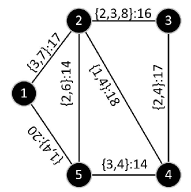
(a) $\mathcal{H}_{1}$ with $k=14$

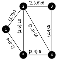
(b) $(4,3)$-truss in $\mathcal{H}_{1}$

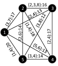
(c) $\mathcal{H}_{2}$ with $k=9$

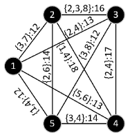
(d) $(12,3)$-truss in $\mathcal{H}_{2}$

Figure 7. The search process of local strategy for Figure1(a)

C.2. The example of TTS algorithm

Table 4 shows the temporal trussness recorded in TT-index for the triangles and edges in the temporal graph $\mathcal{G}$ (Figure1(a)). Consider temporal graph $\mathcal{G}$ in Figure 1(a), and set $\delta=3$. Algorithm 3 first accesses TT-index to obtain the temporal trussness of the edges induced by query node (e.g., node 1). So $k^{*}=\max$ $\{\tau(\bar{e}(1,2)),\tau(\bar{e}(1,3)),\tau(\bar{e}(1,4)),\tau(\bar{e}(1,5)),\tau(\bar{e}(1,6)),\tau(\bar{e}(1,7))\}=12$ and $Q$ is initialized as $\{\bar{e}(1,2),\bar{e}(1,3),\bar{e}(1,4),\bar{e}(1,5)\}$ (i.e. the solid edges in Figure8(a)). Then, for each edge (e.g., $\bar{e}(1,2)$) in $Q$, the algorithm accesses the edges that are in the same triangle with $\bar{e}(1,2)$, and then checks whether the temporal trussness of another two edges is no less than $k^{*}$. As a result, edges $\{\bar{e}(1,3),\bar{e}(2,3),\bar{e}(1,5),\bar{e}(2,5),\bar{e}(1,4),\bar{e}(2,4)\}$ are added into the solution $Q$ because of $\bar{e}(1,2)$ (Figure8(b)). Figure8(c) and Figure8(d) show the temporal subgraph searched by $\bar{e}(1,3)$ and $\bar{e}(1,4)$ step by step, respectively. Finally, this search process terminates when $Q$ is empty and returns Figure8(d) as the final solution.

Table 4. TT for $\mathcal{G}$ in Figure1(a)

$\bar{e}$	TT[e]	$\triangle$	TT[$\triangle$]
$\bar{e}(1,2)$	(1,3),(2,6),(3,12),(4,15),(5,18),(6,22),(7,24)	$\triangle_{123}$	$\delta$=1
$\bar{e}(1,3)$	(1,3),(2,6),(3,12),(4,15),(5,18),(6,22),(7,24)	$\triangle_{124}$	$\delta$=2
$\bar{e}(1,4)$	(1,2),(2,6),(3,12),(4,15),(5,18),(6,22),(7,24)	$\triangle_{125}$	$\delta$=2
$\bar{e}(1,5)$	(1,2),(2,6),(3,12),(4,15),(5,18),(6,22),(7,24)	$\triangle_{126}$	$\delta$=1
$\bar{e}(1,6)$	(1,2),(2,3),(3,5),(4,6),(5,8)	$\triangle_{134}$	$\delta$=1
$\bar{e}(1,7)$	(1,2),(2,8)	$\triangle_{135}$	$\delta$=1
$\bar{e}(2,3)$	(1,3),(2,7),(3,12),(4,15),(5,18),(6,22),(7,24)	$\triangle_{145}$	$\delta$=1
$\bar{e}(2,4)$	(1,2),(2,7),(3,12),(4,15),(5,18),(6,22),(7,24)	$\triangle_{157}$	$\delta$=1
$\bar{e}(2,5)$	(1,2),(2,7),(3,12),(4,15),(5,18),(6,22),(7,24)	$\triangle_{167}$	$\delta$=2
$\bar{e}(2,6)$	(1,2),(2,3),(3,5),(4,6),(6,8)	$\triangle_{234}$	$\delta$=1
$\bar{e}(3,4)$	(1,3),(2,7),(3,12),(4,15),(5,18),(6,22),(7,24)	$\triangle_{235}$	$\delta$=1
$\bar{e}(3,5)$	(1,3),(2,7),(3,12),(4,15),(5,18),(6,22),(7,24)	$\triangle_{245}$	$\delta$=2
$\bar{e}(4,5)$	(1,3),(2,7),(3,12),(4,15),(5,18),(6,22),(7,24)	$\triangle_{345}$	$\delta$=1
$\bar{e}(5,7)$	(1,2),(2,8)	$\triangle_{678}$	$\delta$=2
$\bar{e}(6,7)$	(2,2),(3,4),(4,7),(5,10),(6,12)
$\bar{e}(6,8)$	(2,1),(3,4),(4,7),(5,10),(6,12)
$\bar{e}(7,8)$	(2,1),(3,4),(4,7),(5,10),(6,12)

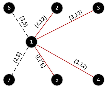
(a) Access TT to initial Q

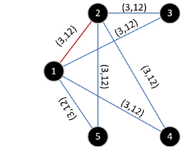
(b) Subgraph searched with $\bar{e}(1,2)$

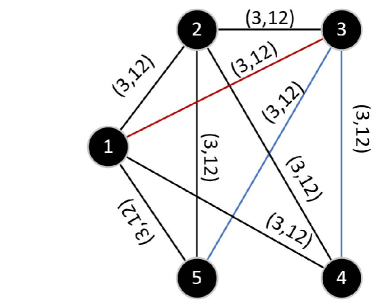
(c) Subgraph searched with $\bar{e}(1,3)$

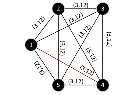
(d) q-MDT searched with $\bar{e}(1,4)$

Figure 8. The illustration of TTS algorithm

Appendix D Theorem Analysis

D.1. Proofs

Here, we provide the proofs of Proposition 4, 5, and 6 in sequence.

Proof of Proposition 4: Time interval $[i,i+\delta+1]$ can be split into two $\delta$-length time intervals: $[i,i+\delta]$, $[i+1,i+\delta+1]$ which correspond to two adjacent temporal subgraphs of $\mathcal{G}^{\delta}$. To compute the number of temporal triangles induced by $\triangle$ in $[i,i+\delta+1]$, we can compute the number of $\tilde{\triangle}$ appearing in $\mathcal{G}_{i}$ and $\mathcal{G}_{i+1}$ separately and then sum them. However, temporal subgraphs $\mathcal{G}_{i},\mathcal{G}_{i+1}\in\mathcal{G}^{\delta}$ overlap in $[i+1,i+\delta]$. So, they have an overlapping temporal subgraph $\mathcal{G}_{[i+1,i+\delta]}$, which is a temporal subgrpah in $(\delta-1)$-slice. Hence, the sum of them will count $N_{\mathcal{G}_{[i+1,i+\delta]}}(\triangle,\delta-1)$ twice. So,

(5) $$N_{\mathcal{G}_{[i,i+\delta+1]}^{\delta}}=N_{\mathcal{G}_{i}^{\delta}}(\triangle,\delta)+N_{\mathcal{G}_{i+1}^{\delta}}(\triangle,\delta)-N_{\mathcal{G}_{i+1}^{\delta-1}}(\triangle,\delta-1)$$

For brevity, let $\Phi_{N_{\mathcal{G}_{i}^{\delta}}(\triangle,\delta)}$=$N_{\mathcal{G}_{i}^{\delta}}(\triangle,\delta)$-$N_{\mathcal{G}_{i}^{\delta-1}}(\triangle,\delta-1)$. Proposition 4 shows that we can know the number of temporal triangles satisfy $\Delta(\tilde{\triangle})\leq\delta$ in next time interval by summing the number of triangles in the current time interval and the difference value between the temporal triangle numbers in corresponding subgraphs of ($\delta$-1)-slice and $\delta$-slice. So, we can extend the proposition to the entire temporal graph and compute the total number of temporal triangle satisfy $\Delta(\tilde{\triangle})\leq\delta$ in the temporal graph $\mathcal{G}$.

Proof of Proposition 5: For concise presentation, we let $N_{\mathcal{G}}$ denote $N_{\mathcal{G}}(\triangle,\delta)$. Similarly, $N_{\mathcal{G}_{i}^{\delta-1}}$ denotes $N_{\mathcal{G}_{i}^{\delta-1}}(\triangle,\delta-1)$. According to Proposition 4, $\forall\triangle\subseteq\mathcal{G}$ and an integer $\delta$, there exists an overlap between two adjacent temporal subgraphs of $\mathcal{G}^{\delta}$ when we compute $N(\triangle)$ of a triangle. So,

(6) $$N_{\mathcal{G}}(\triangle,\delta) =N_{\mathcal{G}_{[1,\delta+1]}}+N_{\mathcal{G}_{[2,\delta+2]}}-N_{\mathcal{G}_{[2,\delta+1]}}+...$$

$$+N_{\mathcal{G}_{[t_{max}-\delta,t_{max}]}}-N_{\mathcal{G}_{[t_{max}-\delta,t_{max}-1]}}$$

$$=N_{\mathcal{G}_{1}^{\delta}}+\sum_{i=2}^{t_{max}-\delta}(N_{\mathcal{G}_{i}^{\delta}}-N_{\mathcal{G}_{i}^{\delta-1}}(\triangle,\delta-1))$$

$$=N_{\mathcal{G}_{1}^{\delta}}+\sum_{i=2}^{t_{max}-\delta}\Phi_{N_{\mathcal{G}_{i}^{\delta}}(\triangle,\delta)}$$

Similarly,

(7) $$N_{\mathcal{G}}(\triangle,\delta-1) =N_{\mathcal{G}_{[1,\delta-1]}}(\triangle,\delta)+\sum_{i=2}^{t_{max}-\delta+1}(N_{\mathcal{G}_{i}^{\delta-1}}-N_{\mathcal{G}_{i}^{\delta-2}}(\triangle,\delta-2))$$

$$=N_{\mathcal{G}_{1}^{\delta-1}}+\sum_{i=2}^{t_{max}-\delta+1}\Phi_{N_{\mathcal{G}_{i}^{\delta-1}}(\triangle,\delta-1)}$$

Therefore,

(8) $$N_{\mathcal{G}}(\triangle,\delta)-N_{\mathcal{G}}(\triangle,\delta-1)=\sum_{i=1}^{t_{max}-\delta}(\Phi_{N_{\mathcal{G}_{i}^{\delta}}(\triangle,\delta)}-\Phi_{N_{\mathcal{G}_{i+1}^{\delta-1}}(\triangle,\delta-1)})~{}~{}~{}~{}~{}~{}~{}~{}~{}~{}~{}~{}$$

So, the Proposition 5 holds.

Proof of Proposition 6: After knowing $N_{\mathcal{G}}(\triangle,\delta)$ of the triangles, we can compute the temporal support of a non-temporal edge as follows.

Proof 1.

For an edge $\bar{e}\in\mathcal{G}$, the temporal support $TSup_{\mathcal{G}}(\bar{e})=\sum_{j=1..n}N_{\mathcal{G}}(\triangle_{j})$, then we have Equation 9. And then the Proposition 6 is proved.

(9) $$TSup_{\mathcal{G}}(\bar{e},\delta) =\sum_{j=1}^{n}N_{\mathcal{G}}(\triangle_{j},\delta)$$

$$=\sum_{j=1}^{n}(N_{\mathcal{G}}(\triangle_{j},\delta-1)+\sum_{i=1}^{t_{max}-\delta}(\Phi_{N_{\mathcal{G}_{i}^{\delta}}(\triangle_{j},\delta)}-\Phi_{N_{\mathcal{G}_{i+1}^{\delta-1}}(\triangle_{j},\delta-1)}))$$

$$=TSup_{\mathcal{G}}(\bar{e},\delta-1)+\sum_{j=1}^{n}\sum_{i=1}^{t_{max}-\delta}(\Phi_{N_{\mathcal{G}_{i}^{\delta}}(\triangle_{j},\delta)}-\Phi_{N_{\mathcal{G}_{i+1}^{\delta-1}}(\triangle_{j},\delta-1)})$$

D.2. Complexity Analysis

Here, we present the complexity of the previous algorithm.

Time complexity of Sliding Window: There are at most $t_{max}$ timestamps, so the window in this edge at most slides $t_{max}$ times. For each temporal edge of $e_{1}$, there are two $\delta$-windows on $e_{2}$ and $e_{3}$, which at most access the edges $\delta^{2}$ times. So, assume there exist at most $t_{max}$ timestamps in $\mathcal{G}$, the time complexity of Sliding Window is ${O}(t_{max}\delta^{2})$.

Time complexity of LS: It is obvious that for each query node, Algorithm 5 accesses at most $|{\{\bar{e}(u,v)|TSup_{{\mathcal{G}}}(\bar{e})>k^{*}\}}|$ edges to compute their temporal support. Besides, counting temporal support requires calling Sliding Window procedure for the triangles who include the edge satisfies that $TSup_{{\mathcal{G}}}(\bar{e})\geq k^{*}$. And checking connection from the decompose’s residual temporal suabgrpah requires accessing fewer edges than the expanded temporal subgraphs. So The time complexity of Algorithm 4 is $O(\sum_{\{\bar{e}(u,v)|TSup_{{\mathcal{G}}}(\bar{e})>k^{*}\}}\min(\mathcal{D}(u),\mathcal{D}(v))+$ $|\{\triangle_{\bar{e}_{1}\bar{e}_{2}\bar{e}_{2}}|TSup_{{\mathcal{G}}}\\ (\bar{e}_{i})>k^{*},1\leq i\leq 3\}|)$.

Complexity of TT-index: For each temporal subgraph $\mathcal{G}_{t}^{\delta}\in\delta$-slice, Algorithm 2 needs to update the $N_{\mathcal{G}_{t}^{\delta}}(\triangle)$ and $TSup_{\mathcal{G}_{t}^{\delta}}(\bar{e})$ for the triangles and edges influenced by the new inserted edges, respectively. Besides, accumulate the increment of the temporal support to gets the final temporal support needs to access at most all the triangles in $\mathcal{G}$. And then, employing the Algorithm decompose takes $\sum_{\bar{e}(u,v)\in\mathcal{G}}\min(\mathcal{D}(u),\mathcal{D}(v))$ time. Therefore, given $\delta$, the update operation spends $\sum_{t=0}^{t_{max}-\delta_{i}}$ $\sum_{\bar{e}(u,v)\in{G}_{[t+\delta,t+\delta]}}$ $\min(\mathcal{D}_{\mathcal{G}_{t}^{\delta}}(u),\mathcal{D}_{\mathcal{G}_{t}^{\delta}}(v))+|\triangle_{\mathcal{G}}|+\sum_{\bar{e}(u,v)\in\mathcal{G}}\min(\mathcal{D}(u),\mathcal{D}(v))$. Since $\delta$ varies from $0$ to $t_{max}$, thus the complexity for constructing TT is $O(\sum_{\delta=0}^{t_{max}}(\sum_{t=1}^{t_{max}-\delta}\sum_{\bar{e}(u,v)\in\mathcal{G}_{[t+\delta,t+\delta]}}\min(\mathcal{D}_{\mathcal{G}_{t}^{\delta}}(u),\mathcal{D}_{\mathcal{G}_{t}^{\delta}}(v))+|\triangle_{\mathcal{G}}|+\sum_{\bar{e}(u,v)\in\mathcal{G}}\min(\mathcal{D}(u),\mathcal{D}(v))))$.

Appendix E Details of Experiments

E.1. Experimental Setting

Datasets. The nine real-world datasets used in our experiments are outlined in Table 5. These datasets are sourced from four distinct domains. Specifically, Rmin, Primary, Lyon and Thiers datasets record face-to-face interactions between students and teachers at different schools (college, high school and primary school). Twitter and Facebook datasets represent popular social networks where users are vertices and interactions are edges. Enron is a dataset which consists of email communications from the Enron company. Lkml is a dataset that captures Linux kernel patchwork and related discussion recorded by the Linux kernel mailing list. DBLP documents scientific collaboration among scholars, providing a comprehensive record of co-authored publications.

Table 5. Dataset Statistics. $TS$ is the time scale of the timestamp.

Dataset	$|V|$	$|\mathcal{G}|$	$|\bar{\mathcal{G}}|$	$|T|$	$TS$
Rmin	96	76,551	2,539	5,576	Hour
Primary	242	26,351	8,317	20	Hour
Lyon	242	218,503	26,594	20	Hour
Thiers	328	352,374	43,496	50	Hour
Twitter	304,198	464,653	452,202	7	Day
Facebook	45,813	461,179	183,412	223	Week
Enron	86,978	697,956	297,456	177	Week
Lkml	26,885	328,092	159,996	98	Month
DBLP	1,729,816	12,007,380	8,546,306	72	Year

Baseline Models. MAPPR (Yin et al., 2017) and k-truss (Huang et al., 2014) are static models which capture the higher-order cohesiveness of the subgraphs in non-temporal networks. OL (Chu et al., 2019) models the dense temporal subgraphs which have the maximal burstness. PCore explores the largest temporal subgraphs that satisfy persistence constraints (Li et al., 2018). DCCS (Zhu et al., 2018) and FirmCore (Hashemi et al., 2022) extend the static core model in multilayer networks to detect the cohesive temporal subgraphs. L-MEGA (Fu et al., 2020) aims to find the communities with higher-order motif on time-evolving graphs.

Settings. All experiments were executed on a server with an Xeon 2.00GHz and 256GB memory running Ubuntu 18.04. All methods are implemented in C++.

E.2. Scalability Evaluation

In order to evaluate the scalability of our methods, we randomly extracted 20%, 40%, 60%, and 80% nodes from DBLP to generate synthetic networks. The query times on these synthetic networks are shown in Figure9. Figure9(a) shows that the running time of GS and LS increases non-linearly as the number of nodes varies, consistent with their time complexity. In contrast, the running time of TTS shows an approximately linear increase with the number of nodes. As shown in Figure9(b), the running time of GS and LS is sensitive to changes in time scale (TS) ranging from 1 year to 5 years, whereas TTS remains stable. Hence, TTS demonstrates efficient handling of large-scale temporal graphs.

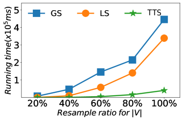
(a) Running time with varying $|V|$

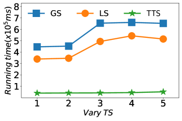
(b) Running time with varying $TS$

Figure 9. Scalability Testing

References

- (1)
- Akbas and Zhao (2017) Esra Akbas and Peixiang Zhao. 2017. Truss-based community search: a truss-equivalence based indexing approach. PVLDB 10, 11 (2017), 1298–1309.
- Andersen and Chellapilla (2009) Reid Andersen and Kumar Chellapilla. 2009. Finding dense subgraphs with size bounds. In International workshop on algorithms and models for the web-graph. 25–37.
- Barbieri et al. (2015) Nicola Barbieri, Francesco Bonchi, Edoardo Galimberti, and Francesco Gullo. 2015. Efficient and effective community search. DMKD 29, 5 (2015), 1406–1433.
- Bogdanov et al. (2011) Petko Bogdanov, Misael Mongiovì, and Ambuj K Singh. 2011. Mining heavy subgraphs in time-evolving networks. In ICDM. 81–90.
- Chang and Qin (2019) Lijun Chang and Lu Qin. 2019. Cohesive subgraph computation over large sparse graphs. In ICDE. 2068–2071.
- Chang et al. (2013) Lijun Chang, Jeffrey Xu Yu, Lu Qin, Xuemin Lin, Chengfei Liu, and Weifa Liang. 2013. Efficiently computing k-edge connected components via graph decomposition. In SIGMOD. 205–216.
- Chen et al. (2020) Lu Chen, Chengfei Liu, Rui Zhou, Jiajie Xu, Jeffrey Xu Yu, and Jianxin Li. 2020. Finding effective geo-social group for impromptu activities with diverse demands. In SIGKDD. 698–708.
- Cheng et al. (2011) James Cheng, Yiping Ke, Shumo Chu, and M. Tamer Özsu. 2011. Efficient core decomposition in massive networks. In ICDE. 51–62.
- Chu et al. (2019) Lingyang Chu, Yanyan Zhang, Yu Yang, Lanjun Wang, and Jian Pei. 2019. Online density bursting subgraph detection from temporal graphs. PVLDB 12, 13 (2019), 2353–2365.
- Cohen (2008) Jonathan Cohen. 2008. Trusses: Cohesive subgraphs for social network analysis. National security agency technical report 16, 3.1 (2008).
- Cui et al. (2014) Wanyun Cui, Yanghua Xiao, Haixun Wang, and Wei Wang. 2014. Local search of communities in large graphs. In SIGMOD. 991–1002.
- Fang et al. (2020) Yixiang Fang, Xin Huang, Lu Qin, Ying Zhang, Wenjie Zhang, Reynold Cheng, and Xuemin Lin. 2020. A survey of community search over big graphs. The VLDB Journal 29, 1 (2020), 353–392.
- Fortunato (2009) Santo Fortunato. 2009. Community detection in graphs. Physics Reports 486, 3 (2009), 75–174.
- Fu et al. (2020) Dongqi Fu, Dawei Zhou, and Jingrui He. 2020. Local Motif Clustering on Time-Evolving Graphs. In SIGKDD. 390–400.
- Gao et al. (2020) Zheng Gao, Hongsong Li, Zhuoren Jiang, and Xiaozhong Liu. 2020. Detecting User Community in Sparse Domain via Cross-Graph Pairwise Learning. In SIGIR. 139–148.
- Goldberg (1984) AV Goldberg. 1984. Finding a maximum density subgraph. Uni. California, Berkeley (1984).
- Han et al. (2016) Zhongming Han, Xusheng Tan, Yan Chen, and Dagao Duan. 2016. NCSS: An effective and efficient complex network community detection algorithm. Scientia Sinica Informationis 46, 4 (2016), 431–444.
- Hashemi et al. (2022) Farnoosh Hashemi, Ali Behrouz, and Laks V. S. Lakshmanan. 2022. FirmCore Decomposition of Multilayer Networks. In WWW. 1589–1600.
- He et al. (2024) Yue He, Longlong Lin, Pingpeng Yuan, Ronghua Li, Tao Jia, and Zeli Wang. 2024. CCSS: Towards conductance-based community search with size constraints. Expert Syst. Appl. 250 (2024), 123915.
- Hong et al. (2022) Jiwon Hong, Dong-hyuk Seo, Jeewon Ahn, and Sang-Wook Kim. 2022. GraphReformCD: Graph Reformulation for Effective Community Detection in Real-World Graphs. In WWW. 180–183.
- Huang et al. (2014) Xin Huang, Hong Cheng, Lu Qin, Wentao Tian, and Jeffrey Xu Yu. 2014. Querying k-truss community in large and dynamic graphs. In SIGMOD. 1311–1322.
- Li et al. (2015) Rong-Hua Li, Lu Qin, Jeffrey Xu Yu, and Rui Mao. 2015. Influential Community Search in Large Networks. PVLDB 8, 5 (2015), 509–520.
- Li et al. (2018) Rong-Hua Li, Jiao Su, Lu Qin, Jeffrey Xu Yu, and Qiangqiang Dai. 2018. Persistent Community Search in Temporal Networks. In ICDE. 797–808.
- Li et al. (2017) Yuan Li, Yuhai Zhao, Guoren Wang, Feida Zhu, Yubao Wu, and Shengle Shi. 2017. Effective k-vertex connected component detection in large-scale networks. In DASFAA. 404–421.
- Lin et al. (2024a) Longlong Lin, Tao Jia, Zeli Wang, Jin Zhao, and Rong-Hua Li. 2024a. PSMC: Provable and Scalable Algorithms for Motif Conductance Based Graph Clustering. CoRR abs/2406.07357 (2024).
- Lin et al. (2023) Longlong Lin, Ronghua Li, and Tao Jia. 2023. Scalable and Effective Conductance-Based Graph Clustering. In AAAI. 4471–4478.
- Lin et al. (2022a) Longlong Lin, Pingpeng Yuan, Rong-Hua Li, and Hai Jin. 2022a. Mining Diversified Top-r Lasting Cohesive Subgraphs on Temporal Networks. IEEE Trans. Big Data 8, 6 (2022), 1537–1549.
- Lin et al. (2022b) Longlong Lin, Pingpeng Yuan, Rong-Hua Li, Jifei Wang, Ling Liu, and Hai Jin. 2022b. Mining Stable Quasi-Cliques on Temporal Networks. IEEE Trans. Syst. Man Cybern. Syst. 52, 6 (2022), 3731–3745.
- Lin et al. (2024b) Longlong Lin, Pingpeng Yuan, Rong-Hua Li, Chun-Xue Zhu, Hongchao Qin, Hai Jin, and Tao Jia. 2024b. QTCS: Efficient Query-Centered Temporal Community Search. Proc. VLDB Endow. 17, 6 (2024), 1187–1199.
- Liu et al. (2020) Qing Liu, Minjun Zhao, Xin Huang, Jianliang Xu, and Yunjun Gao. 2020. Truss-based community search over large directed graphs. In SIGMOD. 2183–2197.
- Ma et al. (2017) Shuai Ma, Renjun Hu, Luoshu Wang, Xuelian Lin, and Jinpeng Huai. 2017. Fast computation of dense temporal subgraphs. In ICDE. 361–372.
- Newman (2004) Mark EJ Newman. 2004. Fast algorithm for detecting community structure in networks. Physical review E 69, 6 (2004), 066133.
- Paranjape et al. (2017) Ashwin Paranjape, Austin R. Benson, and Jure Leskovec. 2017. Motifs in Temporal Networks. In WSDM. 601–610.
- Pardalos and Xue (1994) Panos M Pardalos and Jue Xue. 1994. The maximum clique problem. Journal of global Optimization 4, 3 (1994), 301–328.
- Porter et al. (2022) Alexandra M. Porter, Baharan Mirzasoleiman, and Jure Leskovec. 2022. Analytical Models for Motifs in Temporal Networks. In Companion of The Web Conference 2022, Virtual Event / Lyon, France, April 25 - 29, 2022, Frédérique Laforest, Raphaël Troncy, Elena Simperl, Deepak Agarwal, Aristides Gionis, Ivan Herman, and Lionel Médini (Eds.). ACM, 903–909. https://doi.org/10.1145/3487553.3524669
- Qin et al. (2020) Hongchao Qin, Ronghua Li, Ye Yuan, Guoren Wang, Weihua Yang, and Lu Qin. 2020. Periodic communities mining in temporal networks: Concepts and algorithms. TKDE (2020).
- Qin et al. (2019) Hongchao Qin, Rong-Hua Li, Guoren Wang, Lu Qin, Yurong Cheng, and Ye Yuan. 2019. Mining periodic cliques in temporal networks. In ICDE. 1130–1141.
- Qin et al. (2022) Hongchao Qin, Rong-Hua Li, Ye Yuan, Guoren Wang, Weihua Yang, and Lu Qin. 2022. Periodic Communities Mining in Temporal Networks: Concepts and Algorithms. IEEE Transactions on Knowledge and Data Engineering 34, 8 (2022), 3927–3945.
- Rozenshtein et al. (2020) Polina Rozenshtein, Francesco Bonchi, Aristides Gionis, Mauro Sozio, and Nikolaj Tatti. 2020. Finding events in temporal networks: segmentation meets densest subgraph discovery. Knowledge and Information Systems 62, 4 (2020), 1611–1639.
- Tang et al. (2022) Yifu Tang, Jianxin Li, Nur Al Hasan Haldar, Ziyu Guan, Jiajie Xu, and Chengfei Liu. 2022. Reliable Community Search in Dynamic Networks. Proc. VLDB Endow. 15, 11 (2022), 2826–2838.
- Tsourakakis (2015) Charalampos E. Tsourakakis. 2015. The K-clique Densest Subgraph Problem. In WWW. 1122–1132.
- Wang and Cheng (2012) Jia Wang and James Cheng. 2012. Truss Decomposition in Massive Networks. PVLDB 5, 9 (2012), 812–823.
- Wang et al. (2020) Jingjing Wang, Yanhao Wang, Wenjun Jiang, Yuchen Li, and Kian-Lee Tan. 2020. Efficient Sampling Algorithms for Approximate Temporal Motif Counting. In CIKM. 1505–1514.
- Wang et al. (2022) Lili Wang, Chenghan Huang, Ying Lu, Weicheng Ma, Ruibo Liu, and Soroush Vosoughi. 2022. Dynamic Structural Role Node Embedding for User Modeling in Evolving Networks. ACM Trans. Inf. Syst. 40, 3 (2022), 46:1–46:21.
- Wu and Hao (2015) Qinghua Wu and Jin-Kao Hao. 2015. A review on algorithms for maximum clique problems. European Journal of Operational Research 242, 3 (2015), 693–709.
- Yang et al. (2016) Yi Yang, Da Yan, Huanhuan Wu, James Cheng, Shuigeng Zhou, and John C. S. Lui. 2016. Diversified Temporal Subgraph Pattern Mining. In SIGKDD. 1965–1974.
- Yin et al. (2017) Hao Yin, Austin R Benson, Jure Leskovec, and David F Gleich. 2017. Local higher-order graph clustering. In SIGKDD. 555–564.
- Yu et al. (2021) Michael Yu, Dong Wen, Lu Qin, Ying Zhang, Wenjie Zhang, and Xuemin Lin. 2021. On Querying Historical K-Cores. Proc. VLDB Endow. 14, 11 (2021), 2033–2045.
- Yuan et al. (2018) Long Yuan, Lu Qin, Wenjie Zhang, Lijun Chang, and Jianye Yang. 2018. Index-Based Densest Clique Percolation Community Search in Networks. IEEE Trans. Knowl. Data Eng. 30, 5 (2018), 922–935.
- Zhang et al. (2022) Yifei Zhang, Longlong Lin, Pingpeng Yuan, and Hai Jin. 2022. Significant Engagement Community Search on Temporal Networks. In DASFAA. 250–258.
- Zhu et al. (2022) Chun-Xue Zhu, Longlong Lin, Pingpeng Yuan, and Hai Jin. 2022. Discovering Cohesive Temporal Subgraphs with Temporal Density Aware Exploration. J. Comput. Sci. Technol. 37, 5 (2022), 1068–1085.
- Zhu et al. (2018) Rong Zhu, Zhaonian Zou, and Jianzhong Li. 2018. Diversified coherent core search on multi-layer graphs. In ICDE. 701–712.