Double-edged sword: the influence of tidal interaction on stellar activity in binaries

Abstract

Using the LAMOST DR7 low-resolution spectra, we carried out a systematic study of stellar chromospheric activity in both single and binary stars. We constructed a binary sample and a single-star sample, mainly using the binary belt and the main sequence in the Hertzsprung-Russell diagram, respectively. By comparing the $S$ indices between single and binary stars within each color bin, we found for K type stars, binaries exhibit enhanced activity compared to single stars, which could be attributed to the increase in spin rate caused by tidal synchronization or to the interactions of magnetic fields. Both single stars and binaries fall on a common sequence in the activity-period relation, indicating that chromospheric activities of binaries are dominated by the more active components. More intriguingly, in some color ranges, a slight decline of the $S$ index for smaller orbital period was observed for binary stars. Although the possibility of sample selection effects cannot be excluded, this may mark the first example of super-saturation (i.e., caused by reduced active regions) being detected in chromospheric activity, or provide evidence of the suppressing effect on the magnetic dynamo and stellar activities by strong tidal interaction in very close binaries. Our study suggests that tidal interaction acts as a double-edged sword in relation to stellar activities.

1 Introduction

Stellar activities are external manifestation of the induction and relaxation of magnetic fields. According to the dynamo theories, magnetic fields are generated by stellar rotation and convection. In the $\alpha$–$\Omega$ dynamo, magnetic fields primarily arise from differential rotation at the tachocline (Parker, 1955a, b; Noyes et al., 1984; Chabrier & Küker, 2006), while in the turbulent dynamo, magnetic fields result from the interaction of flow turbulence (Durney et al., 1993; Drake et al., 1996). The strength of stellar activities can be traced by X-ray and radio emissions from stellar corona, spectroscopic emission lines (e.g., Ca II H&K, H$\alpha$) from the chromosphere, and optical flares and cool spots from the photosphere, etc.

Most binaries follow the activity-period relation and the relations between different activity proxies established by single stars (Schrijver & Zwaan, 1991; Wright et al., 2011). This implies the activity properties of binaries are governed by the same physical parameters as single stars, including rotation rates, masses, and ages, which may simply be a consequence that the activities of binaries are dominated by the more active component. On the other hand, in close binaries, such as RS Canum Venaticorum (RS CVn), BY Draconis (BY Dra), W Ursae Majoris (W UMa), and Algol binary systems, tidal interaction and angular momentum transfer lead to high rotation rates and thus strong magnetic activities of the components. However, many stars in these binaries, especially RS CVn type binaries, are significantly more active than expected from their rotation rates, called overactive (Rutten, 1987). Possible magnetic interactions between the components may help explain the overactivity, with some observational evidences including extended coronal X-ray emission and the preferential emergence of flux tubes and hot spots on facing hemispheres (Hill & West, 2016).

Therefore, (close) binaries become excellent tracers of the upper limits of stellar activity and can be used to study the mechanism of super-saturation in the activity-period relation, which was explained by convective updrafts or coronal stripping. In the first scenario, nonuniform heating of the convective envelope leads to a poleward migration of active regions, reducing the filling factor of active regions on stellar surface (Vilhu, 1984; Solanki et al., 1997a, b; Stȩpień et al., 2001), while in the second scenario, the fast rotation of a star results in strong centrifugal forces stripping away the outer layers of the corona, reducing the X-ray emitting volume (Jardine & Unruh, 1999; James et al., 2000). Furthermore, binaries can also be used to study the impact of tidal forces on magnetic dynamo. For example, the tidal force may lead to a 1:1 resonant excitation of the oscillation of the $\alpha$-effect, which is capable of exciting the underlying dynamo (Stefani et al., 2016, 2019; Klevs et al., 2023), although this remains a topic of debate (De Jager & Versteegh, 2005; Nataf, 2022; Weisshaar et al., 2023). On the other hand, tidal effects on rising flux tubes can lead to the formation of clusters of flux tube eruptions at preferred longitudes (Holzwarth & Schüssler, 2003a, b). Besides, binaries exhibit scaled-up interactions that may also occur in a star-planet system, providing valuable insights into the habitability of exoplanets.

Recent ground-based and space-borne photometric sky surveys, such as ASAS-SN (Kochanek et al., 2017), ZTF (Bellm et al., 2019), WISE (Wright et al., 2010), Kepler (Borucki et al., 2010), TESS (Ricker et al., 2015), and Gaia (Gaia Collaboration et al., 2016), have provided large numbers of time-series observations of rotational modulators, offering us a great opportunity to investigate stellar magnetic activity and corresponding dynamo process in binaries (e.g., Chahal et al., 2022). In this study, we choose to utilize the spectroscopic data from the Large Sky Area Multi-Object Fiber Spectroscopic Telescope (LAMOST), together with those photometric surveys, to study the activity variation from single stars to binary systems, across a range of stellar rotation rates and temperatures (i.e., masses). This approach will enable us to understand the impact of tidal and magnetic interactions on stellar magnetic activity more comprehensively. The structure of this paper is organized as follows: Section 2 details our sample selection and data reduction process; Section 3 presents the result and discussion; followed is a short summary in Section 4.

2 Targets selection and Methods

2.1 Sample construction

LAMOST is a 4 m quasi-meridian reflecting Schmidt telescope (Cui et al., 2012; Zhao et al., 2012) designed with a wide field of view for astronomical spectroscopic survey. It is renowned for its ability to obtain more than 3000 spectra in a single exposure with a limiting magnitude as faint as $r=$ 19 mag at the low-resolution. It performs both low- and medium-resolution spectral observations with $R\sim$ 1800 and $\sim$ 7500, respectively. The low-resolution spectrum covers a wavelength range from 3690 Å to 9100 Å (Luo et al., 2015), while the medium-resolution spectrum comprises a blue band from 4950 Å to 5350 Å and a red band from 6300 Å to 6800 Å (Wang et al., 2021).

First, we used the machine-learning algorithm Uniform Manifold Approximation and Projection (McInnes & Healy, 2018) to select H$\alpha$ emission spectra from the LAMOST DR7 low-resolution database (see Sun et al., 2021, for more details). This leads to 170,383 spectra showing clear stellar activities. By a further constraint of signal-to-noise ratio (SNR) with SNR_g $>$ 20, we finally derived 18,382 spectra. Second, we excluded Young Stellar Objects (YSOs) from our sample by cross-matching the YSO catalogs from Marton et al. (2016, 2019, 2023) and Gaia Collaboration (2022). Third, we removed subgiants and giants by using the absolute magnitude of $M_{G}<4.5$ mag. In this step, we derived the distance measurements from Gaia EDR3 (Bailer-Jones et al., 2021), and removed the objects with distances larger than 5 kpc and relative parallax uncertainties larger than 0.2. In addition, the reddening $E(B-V)$ was derived from the Pan-STARRS DR1 (PS1) 3D dust map with $E(B-V)=0.884\times$ Bayestar19, the latter being a measure of extinction given by Green et al. (2019). For sources without extinction estimation from the PS1 dust map, we used the SFD dust map (Schlegel et al., 1998) with $E(B-V)=0.884\times E(B-V)_{\rm SFD}$ as a complement and only kept the sources with $E(B-V)$ $<$ 0.1.

After the final manual check of the spectra and the exclusion of bad ones, our dataset includes 7,836 individual stars with a total 8,997 spectra.

2.2 Calculation of $S$ index

We utilized LAMOST spectra to calculate the canonical $S$ index (Vaughan et al., 1978) to describe the emission in the Ca II H and K lines, which is defined as:

$$S=8\alpha\cdot\frac{H+K}{R+V}.$$ (1)

The $H$ and $K$ values represent the total fluxes within the core regions of the Ca II H&K spectral lines. These fluxes are calculated using a triangular integration function, with a Full Width at Half Maximum (FWHM) of 1.09 Å, centered specifically at wavelengths of 3968 Å and 3934 Å for H and K lines, respectively(Figure 1). The parameters $R$ and $V$ correspond to the integrated fluxes within the adjacent pseudo-continuum regions employing a rectangular integration function featuring a width of 20 Å and centered at 4001 Å and 3901 Å, respectively(Figure 1). We adopt a value of 1.8 for $\alpha$ with the LAMOST LRS data as suggested by Karoff et al. (2016).

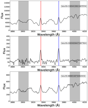
Figure 1: Examples of the LAMOST low-resolution spectra for our sample stars. The red and green lines mark the Ca K and H lines, while the shaded regions represent the spectral range for continuum estimation.

2.3 Stellar rotation periods, orbital periods, and variable types

A number of catalogs, from various photometric/spectroscopic/astrometric sky survey, have provided rotation periods of single stars and orbital periods of binaries, including Kepler (e.g., McQuillan et al., 2013, 2014; Kirk et al., 2016; Santos et al., 2019), K2 (Reinhold & Hekker, 2020), ZTF (Chen et al., 2020), ASAS-SN (e.g., Jayasinghe et al., 2019), Catalina (Drake et al., 2014), WISE (Chen et al., 2018), Gaia (Rimoldini et al., 2023), Gaia DR3 nss_two_body_orbit catalog (Gaia Collaboration et al., 2023), TESS (e.g., Howard et al., 2022; Prša et al., 2022), GCVS (Samus’ et al., 2017), OGLE (Soszyński et al., 2016), LAMOST DR7 (Wang et al., 2022), MEarth (Newton et al., 2016), and HATNet (Hartman et al., 2011). We cross-matched our sample with these catalogs, using a matching radius of 3$\arcsec$, to derive the periods, as well as their stellar variable types. For sources observed by multiple surveys, we selected the periods and variable types based on the priority sequence as mentioned above. This led to 817 rotational single stars and 788 binaries, the latter of which includes 216 eclipsing stars, 28 RS CVn stars, and 544 BY Dra stars.

3 Results and Discussions

In this section, we aim to compare the stellar activity between single and binary stars. In the Hertzsprung-Russell (HR) diagram (Figure 2), the binary belt is clearly visible at 0.75 magnitudes above the main sequence, corresponding to unresolved binaries containing two identical stars, observed with the same color but twice the luminosity of an equivalent single star (Gaia Collaboration et al., 2018). First, we performed a polynomial fitting to the main sequence and derived the equation

$$\begin{split}M_{\rm G}=&0.2339+7.0149\ (G_{\rm BP}-G_{\rm RP})\\ &-2.1773\ (G_{\rm BP}-G_{\rm RP})^{2}\\ &+0.6934\ (G_{\rm BP}-G_{\rm RP})^{3}\\ &-0.07251\ (G_{\rm BP}-G_{\rm RP})^{4}.\end{split}$$ (2)

Second, we selected a binary population and a single-star population from the sample using two slices following the trend of Equation 2. These two populations mainly correspond to the binary belt and the main sequence, respectively. The height of each slice (i.e., the brightness range for the same colour) was set to be 0.6 mag. Between the two slices, we removed a region of 0.15 magnitudes (in height) in order to enhance the distinction between them. This led to 2433 and 3637 stars in the binary and single-star slices, respectively. Although there may be binaries, consisting of a brighter and a fainter star, or triple systems randomly distributed in the HR diagram, the binary fraction in the binary slice is expected to be much higher than that in the single-star slice.

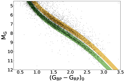
Figure 2: Hertzsprung-Russell diagram of our sample stars. The binary and single-star populations are marked with yellow and green slices, respectively.

Table 1: Stellar parameters of the sample stars.

Gaia ID	R.A.	Decl.	$S$ index	$G_{\rm BP}-G_{\rm RP}$	$M_{G}$	Flaga	Period	Database
	(deg)	(deg)		(mag)	(mag)		(day)
120001145732321536	54.24082	29.28797	0.49	1.01	5.29
219244031627479296	61.29465	35.95703	0.14	0.66	4.62
671703305656347136	116.40658	19.07022	0.96	1.56	7.37
710247613482721536	129.89198	32.86587	0.62	1.43	6.18	b
1783025848682256768	332.34528	22.97542	0.47	1.08	6.04
1894578179565911296	336.72892	30.17105	2.54	1.78	7.96		306.25534	ASAS-SN
2065940880688308480	313.83397	42.56631	0.24	0.82	5.04	s
2067307023883242240	307.39033	39.84348	0.22	1.00	5.80	s
2067556819183564928	306.04291	40.80641	0.14	0.87	4.86	s
2067663540529838592	306.00315	40.89280	0.22	1.03	5.94	s
2069756392191707392	308.15209	43.09314	0.18	1.10	5.38	b
2797676726644861952	3.19585	19.50399	0.35	0.94	5.37
3019756802483967232	92.21274	-6.57617	0.19	0.83	4.86	s
3023162715844336128	85.95600	-5.00640	0.65	1.06	5.23	b
3210609210495286016	81.55687	-4.16286	0.47	1.01	4.62		0.82689	ASAS-SN
3216541728561016704	85.02470	-2.05755	1.40	1.01	4.53		2.39601	ASAS-SN
3327243101868702336	97.99821	9.82066	0.87	1.49	7.18
3377048603487213440	94.71393	22.79092	0.15	0.96	5.05	b
3414109846220439680	77.80178	20.90110	1.64	1.83	8.01
3994816465752179968	165.76459	22.88967	1.23	1.72	6.50
…	…	…	…	…	…	…	…	…

• The flag “b” indicates the star belongs to the binary population (i.e., binary belt), while the flag “s” indicates the star belongs to the single-star population (i.e., main sequence).

This table is available in its entirety in machine-readable and Virtual Observatory (VO) forms in the online journal. A portion is shown here for guidance regarding its form and content.

3.1 Distribution of $S$ index for single stars and binaries

Given the dependence of $S$ index on stellar types (Vaughan & Preston, 1980; Mittag et al., 2013; Boro Saikia et al., 2018), a comparison of $S$ index between the two subsamples (“b” for binaries and “s” for single stars) within the same narrow colour range is necessary. Therefore, we divided each subsample into 10 bins using the colour $G_{\rm BP}-G_{\rm RP}$, ranging from 1.0 to 3.0 with a step of 0.2. Figure 3 displays the distribution of the $S$ index for the two subsamples in each colour bin, and it can be seen that in the color range of 1.0–1.8, mainly consisting of K-type stars, binaries show a higher level of S index compared to single stars. However, when $G_{\rm BP}-G_{\rm RP}>1.8$, their activity levels become indistinguishable.

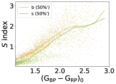
Figure 4: $S$ index versus stellar colour. Left panel: The yellow and green lines represent the median values (Column 50% in Table 2) of the $S$ indices in each colour bin for the binary and single-star samples, respectively. The yellow and green dots correspond to the $S$ indices for the binary and single-star samples. Right panel: The yellow and green lines represent the median values (Column 50%’ in Table 2) of the $S$ indices in each colour bin for the binary and single-star samples, respectively.

Table 2 provides the 50$th$ and 90$th$ percentiles for these distributions. Furthermore, to enhance clarity in the comparison, for the single-star subsample (i.e., subsample “s”), we excluded binaries classified by the catalogs in Section 2.3. Objects with radial velocity variation larger than 10 km/s were also excluded. The corresponding 50$th$ and 90$th$ percentiles of the new $S$-index distributions are flagged as 50%’ and 90%’. Figure 4 displays the relationship between $S$ index and stellar colour, showing that binaries have a higher level of $S$ index compared to single stars when the $G_{\rm BP}-G_{\rm RP}$ color is bluer than $\approx$1.5. More notably, after removing binaries from the single-star slice, the binary belt show a significantly higher level of $S$ index in the color range from 1.0 to 2.5 (Figure 4 right panel).

3.2 Distribution of rotation periods, and orbital periods

To explore the cause of the difference in the $S$-index distribution of binaries and single stars, we examined the distribution of orbital and rotation periods. In Section 2.3, we cross-matched our total sample with some variable catalogs to derive orbital periods for binaries and rotational periods for single stars. However, the binaries and single stars in these catalogs may not be perfectly aligned with the binary and main-sequence slices. This can be due to uncertainties of magnitudes or parallaxes, or misclassifications in these catalogs. To refine the sample, we further cross-matched the binary and single-star slices with the binary sample with orbital periods and the single-star sample with rotational periods. Finally, we analyzed the distribution of orbital periods from 315 binaries in the binary slice and rotational periods from 327 single stars in the main-sequence slice.

Most binaries in our sample have an orbital period less than $\approx$20 days (Figure 5), suggesting the components have been synchronized and the spin period of one or both components equals the orbital period. The period distribution shows that, in the color range of 1.0–1.8, binaries have shorter orbital periods compared to rotational periods of single stars. This helps explain the distribution of $S$ index in Figure 3. For binaries, the tidal interaction plays an important role in influencing stellar evolution through the transfer of angular momentum (de Grijs & Kamath, 2021). On the one hand, orbital synchronization in close binaries can effectively increase stellar spin rate and thus suppress the magnetic braking effect and enhance stellar activity. On the other hand, tidal distortion and magnetic interaction between the components lead to preferential emergence of flux tubes (Holzwarth & Schüssler, 2003a, b), hot spots on facing hemispheres, and extended coronal X-ray emission in RS CVn binaries (Siarkowski et al., 1996), perhaps lasting over a decade. For example, a significant increase in spot coverage was found on the hemisphere facing the white dwarf component in binaries like V426 Oph, SS Cyg, BV Cen, and AE Aqr (Hill & West, 2016).

3.3 Activity-period relation for single stars and binaries

Figure 6 shows the activity-period relation for the sample stars. In each color bin, both single stars and binaries fall on a common sequence in the relation $S$ index versus period. This indicates stellar activities of binaries are mainly governed by the more active component (Schrijver & Zwaan, 2000). For K1–K5 type stars ($G_{\rm BP}-G_{\rm RP}<1.4$), both the saturated regime (i.e., with high and constant activity levels) and the unsaturated regime (i.e., with declining activity levels and periods longer than $\approx$10 days) are observable, while for K6–M4 type stars ($G_{\rm BP}-G_{\rm RP}>1.4$), only the saturated region is evident. The saturation value varies each color bin, ranging from 0.5 ($G_{\rm BP}-G_{\rm RP}=1.0$–1.2) to 2.6 ($G_{\rm BP}-G_{\rm RP}=2.6$–2.8). This variation can be attributed to the thickening of the convective envelope as $T_{\rm eff}$ decreases, leading to a clear increase in the $S$ index.

Interestingly, in some color bins (Figure 6), especially $G_{\rm BP}-G_{\rm RP}=$ 1.2–2.2, there is a slight decline in the saturation limit for binaries with very short orbital periods. We calculated the significance with the following steps. By using the binaries with periods ranging from 0.7 to 7 days, we computed the 50th percentile as the median value and half of the (84th $-$ 16th) percentiles as the standard deviation $\sigma$. Then we calculated the difference between the leftmost black plus and the median value in each panel. We found in all color bins, the significance (i.e., the ratio of the difference to the standard deviation) is approximately 1$\sigma$. Although the significance of the declining trend may not be high, we would still like to provide a brief discussion on the potential mechanisms.

One explanation is the the decline trend is caused by reduced area of active regions, similar to the phenomenon of super-saturation (Prosser et al., 1996). The super-saturation behaviour has been only observed in the X-ray band (e.g. Wright et al., 2011), and its physical origin remains debated. Corresponding theories include decreased filling factor of coronal active regions on the stellar surface (Solanki et al., 1997b; Stȩpień et al., 2001) or reduced X-ray emitting volume due to centrifugal stripping (Jardine & Unruh, 1999; James et al., 2000). In previous studies, the lack of observed super-saturation in chromospheric emission (Cardini & Cassatella, 2007; Mamajek & Hillenbrand, 2008; Marsden et al., 2009; Jackson & Jeffries, 2010) was used to argue in favor of the coronal stripping scenario, since the scenario of the migration of active regions towards the poles could cause super-saturation in chromospheric emission as well. Although we also observe no reduction in the $S$ index for single stars, the binaries in our sample suggest evidence of possible super-saturation in chromospheric emission. Recently, Chahal et al. (2022) found a decline in the saturation value of $S_{\rm ph}$ index for BY Dra-type variables with short periods, most of which are also binaries. Although these authors explained that it was caused by bright faculae partially canceling out dark spots or by the method used to estimate the $S_{\rm ph}$ index, it is also possible that the super-saturation phenomenon is at play. In this case, the super-saturation observed in X-ray, chromospheric, and photospheric activity proxies suggests the decrease in the filling factor of active regions is more likely the mechanism for super-saturation.

Another explanation is that the strong tidal forces may suppress the magnetic activity in very close binaries. As shown in Section 3.1, binaries have enhanced activity compared to single stars due to the increase in spin rate caused by orbital synchronization. However, for very close binary, a more complex situation should be considered. For example, the differential rotation on the surface of the binaries might be suppressed by the tidal forces. Moreover, tidal interactions are expected to induce large-scale 3D shear and/or helical flows in stellar interiors that can notably perturb the stellar dynamo (Alecian et al., 2015). These processes may strongly affect the stellar dynamo and finally the reduce stellar activities.

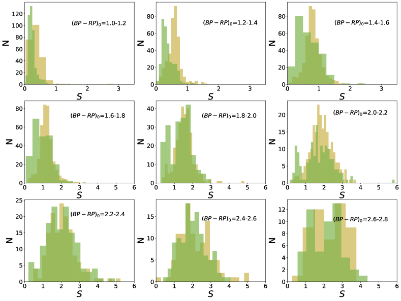
Figure 3: Distributions of the $S$ indices of the two samples in each $G_{\rm BP}-G_{\rm RP}$ bin. The yellow and green histograms represent the binary and single-star samples, respectively.

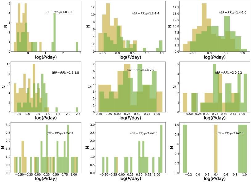
Figure 5: Distributions of rotation periods for single stars and orbital periods for binaries in each $G_{\rm BP}-G_{\rm RP}$ bin. The yellow and green histograms represent the binary and single-star samples, respectively.

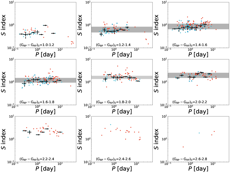
Figure 6: $S$ indices versus rotation periods for single stars (red dots) and orbital periods for binaries. The pluses represent the median $S$ index value in each period bin, and the uncertainties are calculated using the 16th and 84th percentiles. Shaded region indicates the 16th and 84th percentiles of $S$ indices for binaries with periods ranging from 0.7 to 7 days.

$G_{\rm BP}-G_{\rm RP}$	Spec. Type	Flaga	50$\%^{b}$	90$\%^{b}$	N	50$\%$’b	90$\%$’b	N’
1.0-1.2	K1-K3	b	0.35	0.58	234	0.35	0.58	234
		s	0.22	0.48	515	0.21	0.39	447
1.2-1.4	K3-K5	b	0.58	0.78	361	0.58	0.78	361
		s	0.40	0.76	447	0.31	0.63	323
1.4-1.6	K5-K6.5	b	0.80	1.13	435	0.80	1.13	435
		s	0.80	1.25	445	0.62	1.12	260
1.6-1.8	K6.5-K9	b	1.18	1.65	387	1.18	1.65	387
		s	1.08	1.72	352	0.95	1.56	225
1.8-2.0	K9-M1	b	1.53	2.10	280	1.53	2.10	280
		s	1.49	2.21	314	1.37	2.01	204
2.0-2.2	M1-M2	b	1.85	2.66	223	1.85	2.66	223
		s	1.83	2.64	236	1.66	2.66	162
2.2-2.4	M2-M2.5	b	2.00	2.95	149	2.00	2.959	149
		s	2.03	3.18	184	1.95	3.00	142
2.4-2.6	M2.5-M3.1	b	2.01	3.27	107	2.01	3.27	107
		s	2.00	3.04	144	2.00	3.07	113
2.6-2.8	M3.1-M3.5	b	2.13	3.31	51	2.13	3.31	51
		s	2.20	3.32	66	2.17	3.16	52
2.8-3.0	M3.5-M4	b	2.76	3.65	18	2.76	3.65	18
		s	2.40	3.44	28	2.38	3.27	27
total		b	0.95	2.19	2433	0.95	2.19	2433
		s	0.50	2.05	3637	0.31	1.93	2819

• The flag “b” indicates the star belongs to the binary population (i.e., binary belt), while the flag “s” indicates the star belongs to the single-star population (i.e., main sequence).

• The 50% and 90% represent the 50$th$ and 90$th$ percentiles of $S$-index distribution in each color bin, respectively.

Table 2: Distributions of the $S$ indices of the two sliced populations in each $G_{\rm BP}-G_{\rm RP}$ bin.

4 Summary

In this study, we investigated the chromospheric activities of single stars and binaries by using the low-resolution spectra from the LAMOST DR7 dataset. In total, our sample includes 7836 stars with 8997 spectra. The $S$ index was calculated using the Ca II H&K lines for each spectrum. To compare the activities between single and binary stars, we selected two subsamples following the main sequence trend in the HR diagram.

Our results show that, in the $G_{\rm BP}-G_{\rm RP}$ color range of 1.0–1.8 (i.e., mainly K-type stars), binaries tend to exhibit statistically higher levels of activity compared to single stars in the, which could be attributed to tidal synchronization or magnetic field interactions. Simultaneously, binaries do not exhibit double the $S$ index of single stars, suggesting stellar activities of binaries are predominantly governed by the more active component. In the activity-period relation, both single stars and binaries fall on a common sequence, further indicating that the chromospheric activities of binaries are dominated by the more active components.

On the other hand, within certain color ranges, the presence of a super-saturation regime (i.e., a slight decline of the $S$ index for smaller periods) is observed for binary stars. The significance of the super-saturation is not substantial (i.e., about 1$\sigma$), thus a larger sample of binaries with more accurate measurements of chromospheric indices is needed to validate this observation. If the trend is not caused by sample selection effects, this may mark the first observation of super-saturation in chromospheric activity. The super-saturation observed in X-ray, chromospheric, and photospheric activity proxies in recent studies indicates the decrease in the filling factor of active regions is more likely the mechanism for super-saturation. Another explanation for the slight decline trend is that strong tidal forces may significantly affect magnetic dynamo and reduce stellar activities in very close binaries, by suppressing the differential rotation and the convection.

The activity patterns across the HR diagram for close binary stars are more complex than those of single stars, and they are worthy of more detailed future studies, especially with larger binary samples and more accurate activity measurements.

References

- Alecian et al. (2015) Alecian, E., Neiner, C., Wade, G. A., et al. 2015, in New Windows on Massive Stars, ed. G. Meynet, C. Georgy, J. Groh, & P. Stee, Vol. 307, 330
- Bailer-Jones et al. (2021) Bailer-Jones, C. A. L., Rybizki, J., Fouesneau, M., Demleitner, M., & Andrae, R. 2021, AJ, 161, 147
- Bellm et al. (2019) Bellm, E. C., Kulkarni, S. R., Graham, M. J., et al. 2019, PASP, 131, 018002
- Boro Saikia et al. (2018) Boro Saikia, S., Marvin, C. J., Jeffers, S. V., et al. 2018, A&A, 616, A108
- Borucki et al. (2010) Borucki, W. J., Koch, D., Basri, G., et al. 2010, Science, 327, 977
- Cardini & Cassatella (2007) Cardini, D., & Cassatella, A. 2007, ApJ, 666, 393
- Chabrier & Küker (2006) Chabrier, G., & Küker, M. 2006, A&A, 446, 1027
- Chahal et al. (2022) Chahal, D., de Grijs, R., Kamath, D., & Chen, X. 2022, MNRAS, 514, 4932
- Chen et al. (2018) Chen, X., Wang, S., Deng, L., de Grijs, R., & Yang, M. 2018, ApJS, 237, 28
- Chen et al. (2020) Chen, X., Wang, S., Deng, L., et al. 2020, ApJS, 249, 18
- Cui et al. (2012) Cui, X.-Q., Zhao, Y.-H., Chu, Y.-Q., et al. 2012, Research in Astronomy and Astrophysics, 12, 1197
- de Grijs & Kamath (2021) de Grijs, R., & Kamath, D. 2021, Universe, 7, 440
- De Jager & Versteegh (2005) De Jager, C., & Versteegh, G. J. M. 2005, Sol. Phys., 229, 175
- Drake et al. (2014) Drake, A. J., Graham, M. J., Djorgovski, S. G., et al. 2014, ApJS, 213, 9
- Drake et al. (1996) Drake, J. J., Stern, R. A., Stringfellow, G., et al. 1996, ApJ, 469, 828
- Durney et al. (1993) Durney, B. R., De Young, D. S., & Roxburgh, I. W. 1993, Sol. Phys., 145, 207
- Gaia Collaboration (2022) Gaia Collaboration. 2022, VizieR Online Data Catalog, I/358
- Gaia Collaboration et al. (2016) Gaia Collaboration, Prusti, T., de Bruijne, J. H. J., et al. 2016, A&A, 595, A1
- Gaia Collaboration et al. (2018) Gaia Collaboration, Babusiaux, C., van Leeuwen, F., et al. 2018, A&A, 616, A10
- Gaia Collaboration et al. (2023) Gaia Collaboration, Arenou, F., Babusiaux, C., et al. 2023, A&A, 674, A34
- Green et al. (2019) Green, G. M., Schlafly, E., Zucker, C., Speagle, J. S., & Finkbeiner, D. 2019, ApJ, 887, 93
- Hartman et al. (2011) Hartman, J. D., Bakos, G. Á., Noyes, R. W., et al. 2011, AJ, 141, 166
- Hill & West (2016) Hill, M., & West, A. A. 2016, in American Astronomical Society Meeting Abstracts, Vol. 227, American Astronomical Society Meeting Abstracts #227, 145.12
- Holzwarth & Schüssler (2003a) Holzwarth, V., & Schüssler, M. 2003a, A&A, 405, 291
- Holzwarth & Schüssler (2003b) Holzwarth, V., & Schüssler, M. 2003b, A&A, 405, 303
- Howard et al. (2022) Howard, E. L., Davenport, J. R. A., & Covey, K. R. 2022, Research Notes of the American Astronomical Society, 6, 96
- Jackson & Jeffries (2010) Jackson, R. J., & Jeffries, R. D. 2010, MNRAS, 407, 465
- James et al. (2000) James, D. J., Jardine, M. M., Jeffries, R. D., et al. 2000, MNRAS, 318, 1217
- Jardine & Unruh (1999) Jardine, M., & Unruh, Y. C. 1999, A&A, 346, 883
- Jayasinghe et al. (2019) Jayasinghe, T., Stanek, K. Z., Kochanek, C. S., et al. 2019, MNRAS, 486, 1907
- Karoff et al. (2016) Karoff, C., Knudsen, M. F., De Cat, P., et al. 2016, Nature Communications, 7, 11058
- Kirk et al. (2016) Kirk, B., Conroy, K., Prša, A., et al. 2016, AJ, 151, 68
- Klevs et al. (2023) Klevs, M., Stefani, F., & Jouve, L. 2023, Sol. Phys., 298, 90
- Kochanek et al. (2017) Kochanek, C. S., Shappee, B. J., Stanek, K. Z., et al. 2017, PASP, 129, 104502
- Luo et al. (2015) Luo, A. L., Zhao, Y.-H., Zhao, G., et al. 2015, Research in Astronomy and Astrophysics, 15, 1095
- Mamajek & Hillenbrand (2008) Mamajek, E. E., & Hillenbrand, L. A. 2008, ApJ, 687, 1264
- Marsden et al. (2009) Marsden, S. C., Carter, B. D., & Donati, J. F. 2009, MNRAS, 399, 888
- Marton et al. (2016) Marton, G., Tóth, L. V., Paladini, R., et al. 2016, MNRAS, 458, 3479
- Marton et al. (2019) Marton, G., Ábrahám, P., Szegedi-Elek, E., et al. 2019, MNRAS, 487, 2522
- Marton et al. (2023) Marton, G., Ábrahám, P., Rimoldini, L., et al. 2023, A&A, 674, A21
- McInnes & Healy (2018) McInnes, L., & Healy, J. 2018, ArXiv, abs/1802.03426
- McQuillan et al. (2013) McQuillan, A., Aigrain, S., & Mazeh, T. 2013, MNRAS, 432, 1203
- McQuillan et al. (2014) McQuillan, A., Mazeh, T., & Aigrain, S. 2014, ApJS, 211, 24
- Mittag et al. (2013) Mittag, M., Schmitt, J. H. M. M., & Schröder, K. P. 2013, A&A, 549, A117
- Nataf (2022) Nataf, H.-C. 2022, Sol. Phys., 297, 107
- Newton et al. (2016) Newton, E. R., Irwin, J., Charbonneau, D., et al. 2016, ApJ, 821, 93
- Noyes et al. (1984) Noyes, R. W., Hartmann, L. W., Baliunas, S. L., Duncan, D. K., & Vaughan, A. H. 1984, ApJ, 279, 763
- Parker (1955a) Parker, E. N. 1955a, ApJ, 122, 293
- Parker (1955b) Parker, E. N. 1955b, ApJ, 121, 491
- Prosser et al. (1996) Prosser, C. F., Randich, S., Stauffer, J. R., Schmitt, J. H. M. M., & Simon, T. 1996, AJ, 112, 1570
- Prša et al. (2022) Prša, A., Kochoska, A., Conroy, K. E., et al. 2022, ApJS, 258, 16
- Reinhold & Hekker (2020) Reinhold, T., & Hekker, S. 2020, A&A, 635, A43
- Ricker et al. (2015) Ricker, G. R., Winn, J. N., Vanderspek, R., et al. 2015, Journal of Astronomical Telescopes, Instruments, and Systems, 1, 014003
- Rimoldini et al. (2023) Rimoldini, L., Holl, B., Gavras, P., et al. 2023, A&A, 674, A14
- Rutten (1987) Rutten, R. G. M. 1987, A&A, 177, 131
- Samus’ et al. (2017) Samus’, N. N., Kazarovets, E. V., Durlevich, O. V., Kireeva, N. N., & Pastukhova, E. N. 2017, Astronomy Reports, 61, 80
- Santos et al. (2019) Santos, A. R. G., García, R. A., Mathur, S., et al. 2019, ApJS, 244, 21
- Schlegel et al. (1998) Schlegel, D. J., Finkbeiner, D. P., & Davis, M. 1998, ApJ, 500, 525
- Schrijver & Zwaan (1991) Schrijver, C. J., & Zwaan, C. 1991, A&A, 251, 183
- Schrijver & Zwaan (2000) Schrijver, C. J., & Zwaan, C. 2000, Solar and Stellar Magnetic Activity, Cambridge Astrophysics (Cambridge University Press)
- Siarkowski et al. (1996) Siarkowski, M., Pres, P., Drake, S. A., White, N. E., & Singh, K. P. 1996, ApJ, 473, 470
- Solanki et al. (1997a) Solanki, S. K., Motamen, S., & Keppens, R. 1997a, A&A, 324, 943
- Solanki et al. (1997b) Solanki, S. K., Motamen, S., & Keppens, R. 1997b, A&A, 325, 1039
- Soszyński et al. (2016) Soszyński, I., Pawlak, M., Pietrukowicz, P., et al. 2016, Acta Astron., 66, 405
- Stȩpień et al. (2001) Stȩpień, K., Schmitt, J. H. M. M., & Voges, W. 2001, A&A, 370, 157
- Stefani et al. (2016) Stefani, F., Giesecke, A., Weber, N., & Weier, T. 2016, Sol. Phys., 291, 2197
- Stefani et al. (2019) Stefani, F., Giesecke, A., & Weier, T. 2019, Sol. Phys., 294, 60
- Sun et al. (2021) Sun, Y., Cheng, Z., Ye, S., et al. 2021, ApJS, 257, 65
- Vaughan & Preston (1980) Vaughan, A. H., & Preston, G. W. 1980, PASP, 92, 385
- Vaughan et al. (1978) Vaughan, A. H., Preston, G. W., & Wilson, O. C. 1978, PASP, 90, 267
- Vilhu (1984) Vilhu, O. 1984, A&A, 133, 117
- Wang et al. (2021) Wang, S., Zhang, H.-T., Bai, Z.-R., et al. 2021, Research in Astronomy and Astrophysics, 21, 292
- Wang et al. (2022) Wang, Y.-F., Luo, A. L., Chen, W.-P., et al. 2022, A&A, 660, A38
- Weisshaar et al. (2023) Weisshaar, E., Cameron, R. H., & Schüssler, M. 2023, A&A, 671, A87
- Wright et al. (2010) Wright, E. L., Eisenhardt, P. R. M., Mainzer, A. K., et al. 2010, AJ, 140, 1868
- Wright et al. (2011) Wright, N. J., Drake, J. J., Mamajek, E. E., & Henry, G. W. 2011, ApJ, 743, 48
- Zhao et al. (2012) Zhao, G., Zhao, Y.-H., Chu, Y.-Q., Jing, Y.-P., & Deng, L.-C. 2012, Research in Astronomy and Astrophysics, 12, 723