mleMLEMaximum Likelihood Estimate \newabbreviationgmmGMMGeneralized Method of Moments \newabbreviationcgmmCGMMContinuous Generalized Method of Moments \newabbreviationpdf_wordsPDFProbability Density Function \newabbreviationcdf_wordsCDFCumulative Distribution Function \newabbreviationmgf_wordsMGFMoment Generating Function \newabbreviationcf_wordsCFCharacteristic Function \newabbreviationcltCLTCentral Limit Theorem \newabbreviationgcltGCLTGeneralized Central Limit Theorem \newabbreviationedmEDMExponential Dispersion Model \newabbreviationcrCRCramér–Rao \newabbreviationVaRVaRValue at Risk \newabbreviationESESExpected Shortfall \newabbreviationTCETCETail Conditional Expectation \newabbreviationdyDYDevelopment Years \newabbreviationayAYAccident Years \newabbreviationclCLChain Ladder \newabbreviationpcpsPCPsPremium Calculation Principles \newabbreviationcapmCAPMCapital Asset Pricing Model \newabbreviationaptAPTArbitrage Pricing Theory \newabbreviationwipmWIPMWeighted Insurance Pricing Model \newabbreviationabrmABRMAdditive Background Risk Model
Stochastic Loss Reserving: Dependence and Estimation
Abstract Nowadays insurers have to account for potentially complex dependence between risks. In the field of loss reserving, there are many parametric and non-parametric models attempting to capture dependence between business lines. One common approach has been to use additive background risk models (ABRMs) which provide rich and interpretable dependence structures via a common shock model. Unfortunately, ABRMs are often restrictive. Models that capture necessary features may have impractical to estimate parameters. For example models without a closed-form likelihood function for lack of a probability density function (e.g. some Tweedie, Stable Distributions, etc).
We apply a modification of the continuous generalised method of moments (CGMM) of [Carrasco and Florens, 2000] which delivers comparable estimators to the MLE to loss reserving. We examine models such as the one proposed by [Avanzi et al., 2016] and a related but novel one derived from the stable family of distributions. Our CGMM method of estimation provides conventional non-Bayesian estimates in the case where MLEs are impractical.
1 Introduction
Highly regulated and vitally necessary, the loss reserve is typically the largest liability on an insurance company’s balance sheet. Proper estimation of future claims is therefore paramount for financial stability. In fact, with the introduction of regimes like Solvency II actuaries are now sometimes required not just to estimate reserves but model potential shortfalls and risks of insolvency. This makes a stochastic model of loss reserves necessary (see [Wüthrich and Merz, 2008] or [Fröhlich and Weng, 2018] and references therein). This is complicated by the fact that delays between an incurred claim and proper reporting can take some time, often years. There may also be ongoing or renewed liability at a later date for many reasons, such as legal proceedings and lengthy investigations. In the recent past, there have been several high profile examples of these kinds of “tort liabilities” such as asbestos and other environmental pollutants ([Carmean, 1995] and [Madigan and Metzner, 2003]). Newer concerns such as the health risks of engineered materials may present similar issues ([McAlea et al., 2016]). Complicating estimation even further is the potential dependence among claims between business lines. One example that could induce such a dependence may be industry-specific inflationary trends. Medical costs can often rise faster than economy-wide price levels; accident business lines especially may need to incorporate this into their reserves. Similarly, auto repair techniques may incur increased costs for both commercial and personal lines. Such a dependence can represent a potential for diversification or an increased risk to the insurer (see e.g. [De Jong, 2012]).
Given the importance of proper loss reserving it is unsurprising that there are as many forms of reserve estimation as techniques in statistics (see [Wüthrich and Merz, 2008] and references therein). In this paper we focus on the model popularized by [Merz et al., 2013] and model claims parametrically and dependence “cell-wise” across business lines. Within this framework, it is popular to model severity and dependence separately via copulas (e.g. [Zhang and Dukic, 2013]). We instead take a multivariate modelling approach as in [Avanzi et al., 2016]. The benefits and drawbacks of these two approaches (copulas vs multivariate models) are essentially the same as in traditional statistics. Copulas provide a great deal of model flexibility but at the cost of increased numbers of parameters and decreased interpretability. Multivariate models are much more parsimonious but restrict the available marginals.
In order to negotiate this trade-off we construct incremental loss models across business lines via an . ABRMs provide an easily interpretable and flexible dependence through the use of a common shock structure across business lines. The technique can be easily extended to a variety of marginal distributions leading to many possible multivariate models. By way of example, this paper makes use of the multivariate gamma and Tweedie model of, respectively, [Furman and Landsman, 2005] and [Furman and Landsman, 2010] as in [Avanzi et al., 2016] as well as introduces a particular multivariate Stable distribution. The idea of additive risk models is not new in economics and finance. The most famous examples are of course the [Fama and French, 2004] and [Ross, 2013]. More recently the potential for applications in insurance – especially enterprise risk management – has been explored (see e.g. [Furman et al., 2018] and [Zhou et al., 2018]). Other ways to introduce dependence in loss reserves are the Multiplicative Background Risk Models (MBRMs) (e.g., [Furman et al., 2021], [Asimit et al., 2016], [Semenikhine et al., 2018] and [Marri and Moutanabbir, 2022]), minimum-based background risk models (e.g., [Asimit et al., 2010] and [Pai and Ravishanker, 2020]), and background risk models that allow for multiple types of risk factors (e.g., [Su and Furman, 2017a] and [Su and Furman, 2017b]).
The main contribution of our work is not just applying ABRMs but also model estimation. Useful loss models frequently lack a closed form or computationally simple , making classical estimation difficult (e.g. compound Poisson, NIG in the Tweedie case or most non-normal stables). The small sample sizes and many parameters in reserve models naturally lead many to rely on a Bayesian analysis (see for example [Zhang and Dukic, 2013]). There have been attempts to study estimation in the multivariate Tweedie using the method of moments ([Alai et al., 2016]) but for the reasons already stated this seems inappropriate. of [Carrasco and Florens, 2000] offers a hope of success where the basic GMM may fail. Incorporating an infinite number of moment conditions makes the CGMM maximally statistically efficient. In this work we outline a novel use of the CGMM that is relatively computationally inexpensive, especially for “larger” multivariate models. By using the CGMM in conjunction with ABRMs we open up the practical application of a variety of models without the need to resort to highly uncertain Bayesian estimates.
This paper is organized as follows. In Section 2, we give a more detailed account of cell-wise loss modelling and basic estimation. A discussion of what makes a useful model and the introduction of our Tweedie and Stable ABRM examples takes place in Section 3. The CGMM and our novel approach are outlined in Section 4. Finally, some simulation results and an illustration using real data are given in Sections 5 and 6.
2 Parametric Loss-Reserving Models
In this section we briefly review parametric loss-reserving models. Let us consider the following situation. We are in the th accident year since writing a particular non-life policy. We have been able to observe incremental claims for each of 111Year losses were incurred but not necessarily paid. and . We assume that all these are individual samples from random variables that are stochastically independent. We add some necessary structure by enforcing shared parameters in a typical way (see [Wüthrich and Merz, 2008]):
| (2.1) |
where is an appropriate weight and a scale parameter. For some with a of the form , such as Tweedie, Stable, and so on, we can easily construct a for the model parameters:
| (2.2) |
In fact, for Tweedie-distributed incremental losses, estimators of the form (2.2) are numerically similar to the well-known estimators of [Mack, 1993] (see [Mack, 1991] or especially [Taylor, 2009] for more details). Notably, for a Tweedie power parameter of (the overdispersed Poisson) the correspondence is exact. For values “close” to , these estimates are very similar conditional on the scale. For example, if we consider a Gamma model of the form
| (2.3) |
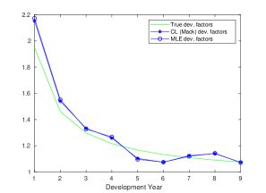
where denotes the reproductive Tweedie density (see A.2 for definitions and details), we can simulate a Gamma-distributed loss development triangle and compare the -derived development factors to those from the estimates in Figure 2.1. It can be seen that the and estimates are virtually identical and both of them are fairly good estimates for the true model.
While the Tweedie class of distributions is quite large, there are some losses for which it is inappropriate. For example, fire and automobile insurance coverage frequently exhibit heavy Pareto-style tails, suggesting an infinite or undefined variance (see [Seal, 1980]). The behaviour of such heavy-tailed distributions is qualitatively different from the typical Tweedie models near (or thin-tailed models generally). One extremely useful and well-motivated model is the Stable distribution. If we repeat our experiment from Figure 2.1 with a stable loss model we can see in Figure 2.2 how the estimates quickly break down.
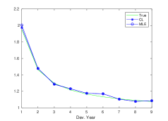
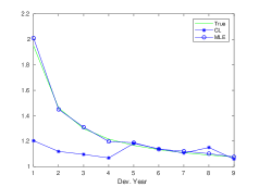
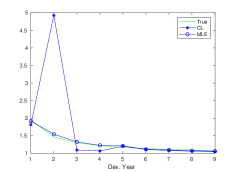
In the stable case, many draws would exhibit fairly typical behaviour (see Figure 2.2a). This is not too surprising as the CL estimates are unbiased provided the mean exists. In the typical case, the sample is mostly represented by the fairly well-behaved centre of the distribution. However, successive draws can reveal that even one or two losses reported out on the tail of the distribution can quickly contaminate the CL estimates, rendering them useless (refer to Figure 2.2b and 2.2c). It is worth pointing out that in Figure 2.2b a major loss early in the development pattern had the unexpected effect of underestimating the development factors. This may not be so obvious in a less marked example when a sample from the tail is creating similar issues. Though the examples chosen are extreme by design, it is easy to see that blind application of non-parametric estimates is ill-advised.
To fully appreciate the implications of heavy tails, we consider that in Figure 2.2c a single cell incurred about 50% of all losses in the triangle. In multiple business lines sharing systematic risk, this can be even more consequential. A single draw from a significantly heavy-tailed risk shared across a portfolio could potentially be greater than the reserve estimated in a thin-tailed model. Such counterintuitive behaviour for heavy tails cannot be ignored.
While a dramatic level of risk exists in heavy-tailed losses, there is hope of overcoming this issue. Unsurprisingly, the MLE estimates in Figure 2.2 are adequate, but this is not without major qualification. First, in order to compute the MLEs one needs a PDF. In the stable case (excepting the Normal distribution), there is no closed-form PDF with finite variance. Calculating the PDF requires the numerical inversion of the or the evaluation of a truncated infinite series to some precision. This numerical quadrature can be very expensive and in the case of multiple business lines is not practical. Additionally, the level of precision required is very high. In the MLEs we studied, we found that the scale parameter was often poorly reported. Furthermore, the method is very sensitive to the choice of initial points used in the optimization. In the case of Figure 2.2b, a few attempts had to be made before producing the results shown.
In this paper we motivate the use of stable loss models. We also extend them to the case of multiple lines of business with a stable . The ABRM has a flexible and easily interpretable dependence structure modelling cell-wise dependence with a multivariate stable distribution. In order to deal with the aforementioned estimation challenges, we make use of the of [Carrasco and Florens, 2000]. These estimates are comparable to MLEs in a more typical case with an order of magnitude fewer calculations. This is achieved by constructing estimators from the directly as opposed to reconstructing a PDF. For example, in the examples above with identical optimization parameters, the CGMM was about thirty times faster than the MLE (60 vs 2000 seconds on a standard IBM ThinkPad). We show that the CGMM makes the multivariate estimation of multiple business lines a practical reality for stable ABRMs.
3 An Additive Background Risk Model
While a single loss development triangle can be used to estimate the required loss reserve facing that line of business, an insurance company typically manages a portfolio of several lines. Given the importance of reserve estimates, dependence between reserves must be modelled. To that end, we identify a few desirable properties of any cell-wise dependent model:
-
•
Marginal flexibility: Any model must capture a large class of possible distributions.
-
•
Closure under marginal convolution: To model sub-portfolios accurately, we must be able to add incremental cells together easily.
-
•
Model confidence: Our model should exist in the limit of a set of reasonable stochastic models, as for example the Normal arises from the . This allows us to feel confident applying the model in general situations.
-
•
Simple and flexible dependence: Any dependence must be transparent and easily interpretable.
To establish our last desired property we introduce an ABRM. The assumptions behind this model are simple. For the th line of business (LoB) of a total of , we assume a cell-wise model of the form
| (3.1) |
That is, we have an independent idiosyncratic component and a “common shock” component across business lines. If we denote
then we can arrange the same cells across business lines into a vector form:
| (3.2) |
where “” denotes the outer product. In this way, we can reduce dependence to the parameters alone. In fact, we can show that for some models (e.g. Normal) this is related to the typical Pearson correlation structure.
The density of such a model can be found by integrating the univariate PDFs à la equation (2.9) in [Avanzi et al., 2016] or equation (6.1) of [Furman and Landsman, 2010]. As the PDFs may not always exist, we are more concerned with the . Letting , we compute the multivariate CF in terms of the univariate CFs:
| (3.3) | ||||
| (3.4) | ||||
| (3.5) |
where denotes the inner product. We can see how the value will control the dependence structure of the distribution. We now move on to some specific examples to illustrate why this representation may be more appropriate.
3.1 Example 1: A Multivariate Tweedie Approach
In our first example we discuss the multivariate Tweedie’s desirable properties. It satisfies the requirements of marginal flexibility and closure under marginals. As discussed, special cases of the Tweedie are the Poisson and Gamma distributions; a more exhaustive list would include the compound Gamma, Normal, and Normal Inverse Gaussian distributions. Additionally, there is a Tweedie class generated by Stable distributions. Being an exponential dispersion model, the multivariate Tweedie has many desirable properties for inference, computation, and interpretation.
We can construct the Tweedie ABRM model in the form of Eq. (3.1), as follows:
| (3.6) | ||||
| (3.7) |
where the additional model parameters are
| (3.8) | ||||
| (3.9) |
This gives us a cell-wise distribution of
| (3.10) |
For various values of the Tweedie power parameter , we lack a closed-form PDF. We can however easily construct the univariate CF via the cumulant function of the Tweedie distribution (see sections (A.1) and (A.2) for details). If , then
where is given by equation A.10.
The universality properties of the Tweedie are perhaps what makes it most applicable to insurance loss modelling. Tweedie distributions are the only EDMs that are closed under rescaling. Take any whose variance is asymptotically a function of the mean such that . This model “converges” in some sense with rescaling to a Tweedie distribution ([Jørgensen, 1987]).
Abusing notation slightly, suppose is a random variable with an exponential dispersion distribution function (A.8). Reading the following equality in the sense of distribution, if
then is Tweedie. EDMs converge under rescaling to Tweedies, in much the same way that Stable variables remain stable under addition and the limit of normalized sums. For any and , suppose (A.9); if as (resp. ), then we have
in distribution as (resp. ). Consider some hypothetical losses incurred according to an EDM with and where is the scale ($1,000’s, $1M’s etc.) as long as the variance remains constant at scale (i.e. ). In this case,
Another example would be for discrete data. Imagine that we are modelling the number of claims in some risk model with distribution , where . Then
A trivial example of this would be if claims were binomially distributed and the number of claims were aggregated or rescaled. The compound Poisson–Gamma is a Tweedie distribution (a compound distribution of two other Tweedies) that may be obtained using this mechanism, which may explain its popularity as a loss model.
3.2 Example 2: A Multivariate Stable Approach
We now consider the most “natural” model that would meet all our required criteria: the multivariate Normal distribution. As the basin of attraction in the Central Limit Theorem, it has the required closure under convolutions and an interpretable linear dependence structure. In fact, for Tweedie power parameter we recover this model.
Since we lack marginal flexibility, the symmetric nature of the Normal makes it awkward for insurance applications. We can however generalize the Normal to the Stable family of distributions. Furthermore, we can consider the class of totally skewed Stables for a more realistic application to insurance. Stables exist as the basin of attraction of sums of heavy-tailed random variables. Thus, given the data compiled by [Eaton et al., 1971] and [Embrechts et al., 2013], Stable models are a good candidate for heavy-tailed insurance portfolios, which cannot be captured by the Tweedie ARBM.
Proceeding in the same way as before,
| (3.11) | ||||
| (3.12) |
we can set
| (3.13) |
In fact we can show that for these parameter values is a true multivariate Stable vector with marginals
| (3.14) |
where the mean, if it exists, is , and we specify scale and importantly the skewness parameter . We consider the special case of maximum skewness i.e. for the rest of the paper as it is the most appropriate for loss modelling. The parameter controls the heavy-tailedness of the distribution.
A Stable model for losses could arise simply through aggregation of smaller losses. Whenever there is an incremental loss, it can be written as the sum of smaller i.i.d. losses :
| (3.15) |
Then by the Generalized Central Limit Theorem (Theorem A.1), we have that weakly where is a standardized Stable distribution:
In both the ABRMs just discussed, we often lack a closed-form PDF of the kind we had in the earlier Gamma model (Eq. (2.3)). In the Stable case, for instance, we only have a closed-form PDF for tail parameters . Unlike our simple example earlier we also have many more parameters across business lines. This further compounds our computational issues.
And yet we have shown such models are desirable. This raises the question: Is there a way of estimating reserves given the observed part of a loss triangle using only what we are guaranteed to have, for example the CF given by Eq. (3.5)? Also, what sacrifices in terms of efficiency would this imply, if any? We explore these issues in the following section.
4 Estimation via Continuous Generalized Method of Moments
4.1 Motivation
As seen in Section 2, given the cell-wise PDF of our claims it is fairly easy to construct maximum likelihood estimators for our model. Unfortunately, as pointed out in the previous section, the ABRMs can lack such a PDF for many parameter values. Indeed, this may make even simple cases (single loss triangles, not too many AY/DYs) computationally expensive. As a point of comparison, one estimation from Table 5.2 in Section 5.1 with identical optimization parameters is about thirty times faster using the continuous generalized method of moments (CGMM) objective than with the MLE objective. This is due to the fact that every evaluation of the PDF/likelihood requires a numerical quadrature of a characteristic or moment function. In multiple lines of business, this is made even worse by the need to add another quadrature for a convolution of univariate PDFs.
In such a case, it may be preferable to seek out alternatives to likelihood estimation. This is the approach adopted by [Avanzi et al., 2016] in relation to [Furman and Landsman, 2010], employing a Markov chain Monte Carlo approach to the completion of a Bayesian analysis. While experience rating can doubtless help the estimation procedure along, we would hope this is not the only recourse available, especially given the often counterintuitive hidden risks of heavy-tailed models specified as in Eq. (3.14).
The only other method of inference introduced in the multivariate Tweedie case is the method of moments (see [Alai et al., 2016]). There has also been much interest in using a method of moments-style estimator for Stable models, but with the characteristic function as a moment condition (see e.g. [Bee and Trapin, 2018] or [Koutrouvelis, 1980]). However, this is inappropriate for loss reserving due to a lack of large enough sample sizes. That said, there is a generalization we may use.
First, let us review the classical introduced by [Hansen, 1982]. The GMM has become overwhelmingly popular in econometrics. This success is in part due to the fairly arbitrary moment conditions required and the lack of distributional assumptions. The GMM can for example handle complex nonlinear regressions involving tricky economic concepts such as endogenous variables.
Unfortunately, the wide applicability of the GMM comes at the cost of statistical efficiency. Because they “throw away” the excess information of perfect specification and introduce ad hoc moment conditions, GMM estimators are widely viewed as less efficient than their more onerous MLE equivalents222There are recent optimal efficiency results (see [Ackerberg et al., 2014] for two-step semi-parametric models) but this is unsurprising as we will shortly see.. This is one reason why we should be skeptical about applying GMM methods to the small samples in loss reserving. That said, it is not hard to show that if the moment conditions are the score of the correctly specified distribution, we actually recover the MLE. To see this, we consider a sample of i.i.d. realizations from some random variable and for specify moment conditions of the form
| (4.1) |
where is a vector-valued function of some model parameters , , , and ; thus Eq. (4.1) is overdetermined333Note abuse of notation: technically we should denote by , but as a set of parameters we want to set it aside for succinctness and to avoid confusion with data and other vectors.. We can take a sample average to approximate (4.1):
| (4.2) |
For some positive definite matrix , we can define an inner product and corresponding norm and minimize the norm of Eq. (4.2) to arrive at the GMM objective function. The GMM estimates for are then444Obviously this is equivalent to , being the transpose.
| (4.3) |
The most statistically efficient matrix is , which is the inverse of the covariance matrix of our moment conditions. We can prove that such estimators exhibit asymptotic normality such that , where is the true parameter value and
| (4.4) |
Where the expectation is w.r.t. and the derivative is understood as the gradient in the case . Interestingly, this suggests that the correct moment conditions can recover the same information that was “thrown away” from the MLE. Indeed, we will see that the result of [Carrasco and Florens, 2000] formalizes just this idea to construct CGMM estimators. For now, let us consider the moment condition of form
| (4.5) |
That is, Eq. (4.5) is the score function. Obviously, will solve Eq. (4.1), while and where is the Fisher information matrix. Therefore . That is, the GMM estimators achieve the bound and are thereby as efficient as the MLEs. The intuition here is unsurprising as we are making use of the same information, namely specification, as in the MLE. In some sense, then, the GMM can be seen as more general than likelihood estimation. The CGMM in turn is a further generalization to a continuum of moment conditions.
4.2 The CGMM
Consider the specific problem of estimating models efficiently from their integral transforms, namely the aforementioned Tweedie and Stable models. In [Feuerverger and McDunnough, 1981], the authors suggested the following moment condition. For we choose a moment condition involving a CF of the form
| (4.6) |
They claimed this could be thought of as a potentially infinitely over-specified moment condition. The idea is that by sampling an increasing number of values and proceeding with the typical GMM, one could achieve the CR bound. However, they did not prove this result, nor did they take into account how to construct the proper covariance matrix in such a way as to continuously match the infinite-dimensional moment condition of Eq. (4.6).
To see why a continuous moment matching is necessary consider the resulting vector-valued function (Eq. (4.2) and covariance matrix:
where
Note that is Hermitian and positive definite, and satisfies properties that we would normally find desirable. However, one can show that the smallest eigenvalue of such a matrix will approach zero as goes to infinity. This will make operations involving and the GMM very unreliable numerically. In fact, if we were to take the limit as approaches infinity, would become unbounded and not invertible. This leaves us in need of a procedure to continuously match our -norm in (4.3) with the moment conditions.
In [Carrasco and Florens, 2000] the authors tackled these problems by inventing the CGMM. Rather than simply sampling from a continuous object as in Eq. (4.6), they reformulated the GMM in continuous terms: vectors and matrices become elements of a Hilbert space and operators, respectively. Intuitively, if we consider instead of a vector moment condition we get a function, so that , specifically a function of .
In the interest of brevity, given a function of several variables we will write integrals like so:
| (4.7) |
To avoid confusion with the discrete inner product above, the inner product for functions and is defined as
| (4.8) |
In order to give the typical notion of , we set
| (4.9) |
the space over which we will primarily be working in the CGMM. Finally, given and a kernel function we will denote the notion of a Fredholm-style operator as
| (4.10) |
By way of example to illustrate the CGMM, we again consider an i.i.d. sample , but this time define the moment condition by a function of :
| (4.11) |
so that
| (4.12) |
And rather than a matrix we define a positive-definite kernel function:
| (4.13) |
We can generalize the GMM estimators to their continuous counterparts:
| (4.14) |
While the operator and its inverse are self-adjoint, the expression is often undefined. The inverse square root of the operator has a larger domain than the simple inverse and that is why we write Eq. (4.14) as here.
Estimators of the kind defined in Eq. (4.14) can be shown to be as efficient as the MLE, achieving the CR bound. The intuition behind this is discussed in [Carrasco et al., 2014]. The GMM can recover the MLE if the moment conditions involve the score; by generalizing the GMM to Hilbert spaces we can relax this. We now only require the new moment conditions to contain the score within their linear closure. Naturally, this is true for moment conditions of form (4.12). Figure 4.1 summarizes the situation.
Evaluating the objective is equivalent to solving a Fredholm integral equation of the first kind. That is, the function can be seen as a solution to the equation
| (4.15) |
where is the integral operator with kernel given by Eq. (4.13).
In what follows, we provide a quick introduction to solving integral equations in a practical way. In general, the true inverse of an operator, namely such that , is unbounded. Solutions of Eq. (4.15) will only be defined for a dense subset of . To ensure existence everywhere, we need to weaken our notion of a solution to one that solves the least squares problem. Therefore, rather than solving , we solve
| (4.16) |
The operator is called the pseudoinverse of . This satisfies the existence problem. Unfortunately, problems of the kind (4.16) are still not well posed. Given especially that our moment conditions (4.12) are estimated from data, we need to introduce the regularized problem that is well posed:
| (4.17) |
This regularized minimization problem has a unique solution , where is the adjoint of . As , we recover (4.16). We can thus think of the regularized problem as approximating an ill-posed problem with a “nearby” well-posed one.
4.3 Loss Reserve Estimates
Let us revisit the example from Section 2 involving the Gamma losses in Figure 2.1. We will compute estimates for , and using the CGMM instead of the MLE. We define the following:
-
•
-
•
so that
-
•
-
•
where
The objective function to be used is
| (4.18) |
Evaluating the using the Nyström method and numerically optimizing (detailed in the next section), we obtain the mean expected claims shown in Table 4.1.
| Accident Year | Realized Losses | Estimated Claims (CGMM) | Estimated Claims (MLE) |
|---|---|---|---|
| 2 | 2.92 | 1.93 | 2.66 |
| 3 | 8.10 | 9.70 | 7.88 |
| 4 | 12.37 | 20.08 | 17.04 |
| 5 | 27.07 | 37.22 | 27.92 |
| 6 | 41.73 | 71.03 | 45.49 |
| 7 | 63.84 | 85.42 | 66.37 |
| 8 | 94.94 | 100.68 | 98.76 |
| 9 | 127.07 | 110.27 | 113.36 |
| 10 | 167.27 | 134.52 | 138.03 |
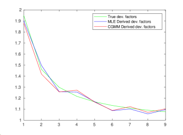
Given that for Tweedie losses with power parameter close to , we expect the CL and MLE estimates to be close, it is unsurprising that the CGMM parametric estimate for the development factors is also similar, as shown in Figure 4.2.
4.4 Numerical Considerations
Estimating the Kernel Function
In both the GMM and the CGMM, we have thus far ignored the estimation of the matrix and the kernel operator respectively. Recall they are defined as the expectation of the Kronecker product of our moment functions, which require the very quantity we are trying to estimate, namely . In the i.i.d. case, the natural choice of estimator is simply
| (4.19) |
where .
Unfortunately, in loss reserving we do not have the luxury of sizable i.i.d. samples. To address this issue, we continuously update the kernel function (defined in (4.13)) after a reasonable initial estimate (e.g. the CL estimates). This strategy is appropriate for the same reason that continuously updating in the discrete GMM case works: as [Carrasco and Florens, 2000] shows, any appropriate kernel function that produces a norm can produce a consistent estimate for . Unfortunately, this does add some computational cost.
Estimation of
The choice of regularization parameter obviously affects the estimators. If it is too large (resp. too small), the problem we are solving is too far from the original regularized problem (resp. we lose numerical stability). We direct the reader to the discussion in [Kotchoni, 2012] for possible simulation-based approaches to optimizing this parameter. In the loss-reserving setting, we find that a good “rule of thumb” is to set when the number of development years is around .
Numerical Integral Equation Solutions 1: The Nyström method
The most obvious way of evaluating (4.15) is via numerical quadrature. We introduce quadrature points555Capital here is taken to be deterministic. and corresponding weights such that
We can then represent the continuous problem of the kind (4.15) as
or more succinctly as . We then evaluate the CGMM objective (4.14) as , where .
Numerical Optimization
Consider a more general moment function of the form
| (4.20) |
Thus far, we have only discussed expressions of the kind leading to , the CF. The CGMM is not limited to such expressions. For example, given a CDF it is just as natural to choose , leading to an equivalent expression of form
| (4.21) |
A closed-form CDF is, of course, lacking in the models we are interested in, so this point may seem moot. However, we emphasize that if the linear closure of expressions of the form contains the score of our distribution, we can employ the CGMM confidently, as demonstrated by the following theorem.
Theorem 4.1 ([Carrasco et al., 2014]).
Consider the subspace of formed by the linear hull of . That is, for consider the space of random variables of the form
and their mean square limits such that
If the score , then the resulting CGMM estimator for is asymptotically as efficient as the MLE.
Thus, for example in one dimension we can use the characteristic function and approximate a limit point in by an integral as follows:
| (where the expectation is w.r.t. , i.e. ) | |||
Theoretically, there are few issues with choosing the CF. Practically speaking, however, the CF may lead to non-convex objectives that are difficult to optimize. For instance, consider the following simple situation. Given an i.i.d. sample of , where with and , and and , we can plot the surface of (4.14) as shown in Figure 4.3a. Keep in mind, we wish to find the minimum.
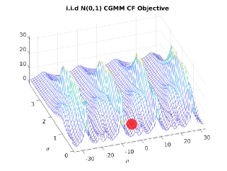
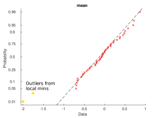
The true minimum (shown by the red dot in Figure 4.3a) is still close to , as expected. We can see however that the presence of complex-valued functions creates oscillations and periodicity. Often, numerical errors and the sheer non-convexity of the objective can lead to standard gradient descent algorithms getting “stuck” out in neighbourhoods of adjacent local minimums. This is especially true in the heavier-tailed case, where it is harder to guess the initial point to start the optimization. To see this, look for instance at the Prob-Prob plot of the sampling distribution for (generated using ()-sized Stable samples with ) in Figure 4.3b. While the distribution appears mostly Normal (which, in theory, would be the case asymptotically) we can see that these numerical issues create a few notable outliers. In [Kotchoni, 2012] the application of the CGMM to heavy-tailed Stable variates required rather large sample sizes to overcome this problem. We suspect that this issue is partly why the CGMM has not yet seen wide application.
In the loss-reserving case, the picture is more challenging. The increased dimensions of the objective and possible local minimums mean that it is a near certainty that standard algorithms will get stuck. Two similar alternative approaches to finding a global minimum that we explore are MATLAB’s built-in scatter-search and genetic algorithms. The former is used to generate the results in our Gamma example of Section 4.3. Both of these algorithms search a larger portion of the feasible space and often produce favourable results. Another useful trick is to add a penalty for solutions found too far away from a good first estimate (say, the chain-ladder parameters). These approaches often produce the true optimum. However, the reality is that the fundamental non-convexity and periodicity of the objective are too much to overcome reliably.
Ideally, we would like to find moment conditions that are not just statistically valid but also produce well-behaved objective functions. It is preferable to make use of integral transforms that produce real and (log-)convex functions such as the moment-generating function. That is,
| (4.22) |
with corresponding kernel function
| (4.23) |
where is the of . However, we run into issues showing this satisfies the conditions of Theorem 4.1. To begin with , if left unrestricted, is no longer in . Additionally, we would require , which has no real coefficients.
In light of this, we can instead perform a “Wick rotation” and recover the MGF that way. Setting , we can make use of (4.22) as long as we keep the CF form for :
| (4.24) |
Using the MGF and this new kernel, we can generate a new objective function as in Figure 4.4 from the same scenario and data used in Figure 4.3a. As we can see, the objective function is now convex and much more amenable to numerical optimization.
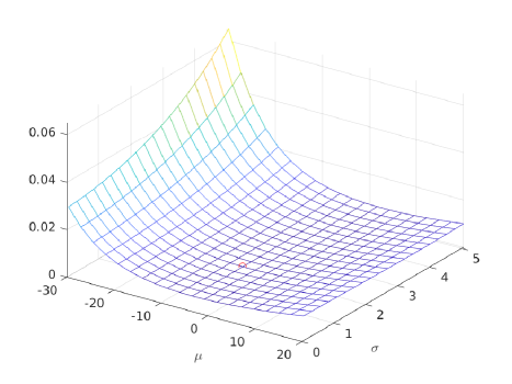
One aspect of note that will reoccur in Section 5.2 is that the objective function has little curvature around the optimum. This “flatness” becomes even more pronounced as we add dimensions to the data (or lines of business in the loss-reserving problem).
Before continuing to numerical examples, we have one additional issue to consider. To guarantee our conditions are properly bounded, we introduce a dampening function. In methods where the empirical characteristic function is used (e.g. kernel density estimation), it is well-known that some values of are unreliable. If we use the MGF instead, the same issue arises but now the actual MGF may not even be defined at some . As a remedy to both issues, dampening functions are employed to emphasize more reliable regions of over others. In our setting, this takes the form
| (4.25) |
where is a dampening function. It is easy to show that this fits well into the CGMM framework. For instance, in [Carrasco and Florens, 2000] this takes the form of a new measure and space where the CGMM results still hold true.
5 Simulation Results
5.1 Single LoB Illustration
For each of the examples discussed in this section, we simulate 50 single LoB (line of business) loss triangles with 10 accident years and 10 development years. For simplicity, we use the same parameter values as in our Gamma examples. We use (4.22) and (4.24) to construct a CGMM objective of the form (4.18). We then find the estimators via MATLAB’s fmincon function, which employs sequential quadratic programming.
Tweedie Losses: Compound Gamma and Gamma
In the univariate case, the (reproductive) MGF of the Tweedie distribution is
| (5.1) |
For some values of , the MGF cannot be defined past some positive . For example, in the (Gamma) case, we require . This may create some issues with the kernel function (recall the argument in the first term). To avoid this we choose a dampening function of the form and consider the MGF only over :
| (5.2) |
Using this formulation, we construct an objective of the form (4.18), but rather than the CF we use the MGF and a kernel of the form (4.23). Integration for is done via a simple trapezoidal scheme 666Interestingly, Newton–Coates schemes require fewer quadrature points than Gaussian quadrature. Despite having the freedom to select any , it appears the function is well-behaved enough that linear approximations are sufficiently precise.
Table 5.1 summarizes the statistics for the CGMM estimates for Tweedie power parameters and . For comparison, we include the chain ladder and MLE estimators, respectively. While the mean parameters of and are slightly biased, the advantage goes to the CGMM in the estimation of the scale. The bias is present in the Stable example as well and we will discuss why in that case. For now, it is likely safe to conclude that the CGMM and CL/MLE estimators are at least comparable.
Stable Losses
Given that Stable variables do not admit even second moments for all but , using the MGF over the CF to generate a CGMM objective in the Stable case seems misguided at first glance. Fortunately, [Eaton et al., 1971] and [Samorodnitsky, 2017] have studied the Laplace transformation of an extreme Stable distribution () and applied the Paley–Wiener theorems to conclude that for the “moment generating function” is given by
| (5.3) |
Note the fact that the resulting cumulant function is similar to the Tweedie, which formalizes the connection we hinted at earlier.
Again, for negative values of this obviously produces complex-valued arguments. Hence, once again we consider only the half-line that works for us. We also multiply by to ensure positive losses:
| (5.4) |
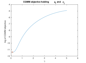
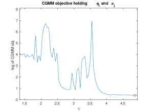
In Figure 5.1, we compare a slice of the CGMM objective using the Stable MGF with another using the CF. As one can see, the difference is quite stark. Again, while a global search may give the correct minimum, it is not difficult to see why the MGF-based moment functions give much better and more consistent performance.
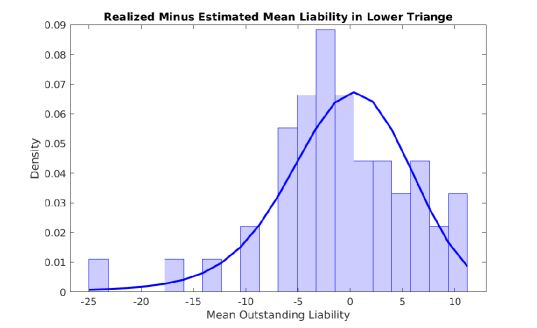
In Table 5.2, the estimates for are slightly biased. This is in turn reflected in a small underestimation of the outstanding losses in Figure 5.2. We suspect this is due to the fact that compared to the MLEs, there is an extra parameter to optimize: the previously discussed regularization parameter . We conduct a crude search by checking which values of give the best performance in a small series of simulations. A more systematic treatment could potentially offer better results and eliminate any bias. As previously mentioned, see discussion in [Kotchoni, 2012] for more on treatment of .
| CGMM | Chain Ladder | CGMM | MLE | ||||||||||
| True | Median | SD | Median | SD | True | Median | SD | Median | SD | ||||
| 5.00 | 4.71 | 0.77 | 5.12 | 1.14 | 5.00 | 4.97 | 2.40 | 4.75 | 1.08 | ||||
| 5.00 | 4.73 | 0.59 | 4.99 | 1.24 | 5.00 | 4.59 | 2.00 | 5.24 | 1.04 | ||||
| 5.00 | 4.84 | 0.76 | 5.05 | 1.17 | 5.00 | 4.35 | 1.67 | 5.12 | 1.10 | ||||
| 5.00 | 4.64 | 0.80 | 4.95 | 1.29 | 5.00 | 4.41 | 2.25 | 5.16 | 1.05 | ||||
| 5.00 | 4.60 | 0.66 | 4.77 | 1.39 | 5.00 | 4.39 | 2.38 | 4.90 | 1.23 | ||||
| 5.00 | 4.79 | 0.92 | 5.23 | 1.44 | 5.00 | 4.82 | 2.42 | 4.72 | 1.20 | ||||
| 5.00 | 4.49 | 0.80 | 4.77 | 1.44 | 5.00 | 4.88 | 2.27 | 5.18 | 1.23 | ||||
| 5.00 | 4.28 | 0.75 | 4.67 | 1.14 | 5.00 | 4.29 | 2.05 | 4.57 | 1.40 | ||||
| 5.00 | 4.29 | 0.91 | 4.69 | 1.20 | 5.00 | 4.52 | 1.75 | 4.67 | 1.42 | ||||
| 5.00 | 4.84 | 0.90 | 5.06 | 1.10 | 5.00 | 4.64 | 1.70 | 4.78 | 1.86 | ||||
| 1.00 | 1.00 | 0.00 | 1.00 | 0.00 | 1.00 | 1.00 | 0.00 | 1.00 | 0.00 | ||||
| 0.95 | 0.97 | 0.08 | 0.92 | 0.12 | 0.95 | 0.90 | 0.12 | 0.94 | 0.15 | ||||
| 0.90 | 0.88 | 0.07 | 0.87 | 0.09 | 0.90 | 0.82 | 0.14 | 0.87 | 0.18 | ||||
| 0.85 | 0.84 | 0.09 | 0.79 | 0.11 | 0.85 | 0.76 | 0.14 | 0.79 | 0.18 | ||||
| 0.80 | 0.82 | 0.09 | 0.77 | 0.11 | 0.80 | 0.74 | 0.14 | 0.77 | 0.18 | ||||
| 0.75 | 0.76 | 0.09 | 0.74 | 0.10 | 0.75 | 0.72 | 0.12 | 0.71 | 0.15 | ||||
| 0.70 | 0.72 | 0.10 | 0.70 | 0.12 | 0.70 | 0.67 | 0.14 | 0.66 | 0.16 | ||||
| 0.65 | 0.68 | 0.11 | 0.66 | 0.11 | 0.65 | 0.68 | 0.17 | 0.63 | 0.22 | ||||
| 0.60 | 0.66 | 0.12 | 0.58 | 0.13 | 0.60 | 0.63 | 0.18 | 0.59 | 0.23 | ||||
| 0.55 | 0.58 | 0.13 | 0.53 | 0.17 | 0.55 | 0.61 | 0.21 | 0.54 | 0.26 | ||||
| 0.20 | 0.22 | 0.10 | 0.08 | 0.07 | 0.20 | 0.19 | 0.11 | 0.13 | 0.03 | ||||
| True | Mean | SD | True | Mean | SD | ||||
| 5 | 4.82 | 0.30 | 1 | 1.00 | 0.00 | ||||
| 5 | 4.78 | 0.28 | 0.95 | 0.96 | 0.04 | ||||
| 5 | 4.80 | 0.26 | 0.9 | 0.92 | 0.04 | ||||
| 5 | 4.84 | 0.25 | 0.85 | 0.86 | 0.05 | ||||
| 5 | 4.83 | 0.30 | 0.8 | 0.81 | 0.05 | ||||
| 5 | 4.79 | 0.23 | 0.75 | 0.75 | 0.04 | ||||
| 5 | 4.80 | 0.28 | 0.7 | 0.70 | 0.05 | ||||
| 5 | 4.80 | 0.27 | 0.65 | 0.66 | 0.05 | ||||
| 5 | 4.84 | 0.25 | 0.6 | 0.59 | 0.06 | ||||
| 5 | 4.82 | 0.27 | 0.55 | 0.54 | 0.07 | ||||
| 0.2 | 0.18 | 0.02 |
5.2 Multiple LoB Illustration
In this section, we extend all the same methods from the single LoB to two LoBs. We simulate 50 joint triangles from a two-dimensional model of the kind specified by (3.2). To create our objective we use a moment condition of the form
For the Stable case, we once again consider evaluating using and the half-plane containing , but a practical problem immediately presents itself. As alluded to in Section 4.4, produces an objective function with little curvature around the optimum, being basically flat for much of its support. Our current workaround to produce the results in Table 5.3 is as follows. First, we make use of a change of variable to concentrate as many of the quadrature points as possible where the function has the most substantial value. Second, we multiply the corresponding objective by a large number. This guarantees that any optimizing algorithm unable to distinguish between a flat region and a very lightly curved one would not terminate prematurely. That being said, formally understanding the relationship between moment conditions and the resulting objective, along with a more systematic approach to numerical optimization, remains an avenue for future work.
The results here are not as precise as in the previous section. However, virtually all parameters are within a standard deviation. Importantly, the CGMM is able to capture the systematic parameters motivating the exercise in the first place.
It goes without saying that the results for the single LoB cases seem more accurate. One aspect of the CGMM we lament is the degree of subjectivity of choices in the methodology. For example, to guarantee that the regularization term and MSE in Eq. (4.17) are balanced (guaranteeing that we converge to the “correct” solution as ), we need to standardize the columns of . In the multiple LoB case, is rather sparse and hence very sensitive to the choice of standardization, dramatically affecting the results. This is an example of the kind of problem we encounter in the multiple LoB case that is either not present or at least not as important as in the single LoB case. Furthermore, practical results (especially vs the MLE) would still take on the order of hours or days to produce, making thorough experimentation slow. That said, we are confident that finding the proper regularization is simply a matter of trial and error.
In the next section, we apply the same method to a well-studied data set, and succeed in producing seemingly favourable results. This suggests even as a preliminary conclusion that the CGMM can compete with existing methods.
| Line 1 | Line 2 | |||||||
| Parameter | True | Median | SD | Parameter | True | Median | SD | |
| 5.00 | 4.42 | 0.35 | 4.00 | 3.78 | 0.52 | |||
| 5.00 | 4.48 | 0.46 | 4.00 | 3.68 | 0.44 | |||
| 5.00 | 4.44 | 0.35 | 4.00 | 3.80 | 0.52 | |||
| 5.00 | 4.40 | 0.39 | 4.00 | 3.94 | 0.47 | |||
| 5.00 | 4.48 | 0.60 | 4.00 | 3.89 | 0.52 | |||
| 5.00 | 4.41 | 0.47 | 4.00 | 3.89 | 0.40 | |||
| 5.00 | 4.43 | 0.40 | 4.00 | 3.85 | 0.39 | |||
| 5.00 | 4.44 | 0.39 | 4.00 | 3.98 | 0.40 | |||
| 5.00 | 4.55 | 0.63 | 4.00 | 3.92 | 0.85 | |||
| 5.00 | 4.66 | 0.31 | 4.00 | 4.02 | 0.43 | |||
| 1.00 | 1.00 | 0.00 | 1.00 | 1.00 | 0.00 | |||
| 0.93 | 1.01 | 0.08 | 0.95 | 0.96 | 0.09 | |||
| 0.87 | 0.95 | 0.07 | 0.90 | 0.92 | 0.10 | |||
| 0.80 | 0.88 | 0.07 | 0.85 | 0.85 | 0.11 | |||
| 0.73 | 0.81 | 0.08 | 0.80 | 0.81 | 0.08 | |||
| 0.67 | 0.73 | 0.06 | 0.75 | 0.76 | 0.09 | |||
| 0.60 | 0.65 | 0.05 | 0.70 | 0.69 | 0.09 | |||
| 0.53 | 0.60 | 0.08 | 0.65 | 0.65 | 0.11 | |||
| 0.47 | 0.51 | 0.06 | 0.60 | 0.56 | 0.10 | |||
| 0.40 | 0.43 | 0.17 | 0.55 | 0.54 | 0.22 | |||
| 0.20 | 0.16 | 0.10 | 0.30 | 0.15 | 0.09 | |||
| Systematic Parameters | ||||||||
| Parameter | 1.00 | Median | SD | |||||
| 0.10 | 0.17 | 0.12 | ||||||
| 0.10 | 0.12 | 0.07 | ||||||
6 Real-world Data Analysis
In this section, we use the data first used in [Zhang and Dukic, 2013] and [Avanzi et al., 2016] from the Pennsylvania National Insurance Group (Schedule P, see Table B.1 and B.2) to study multivariate and copula Tweedie-based loss models from a Bayesian perspective. We estimate every model parameter using our multivariate CGMM methodology except for the Tweedie power parameter , which we set a priori at . This is the value found in [Avanzi et al., 2016], derived from an analysis of the likelihood.
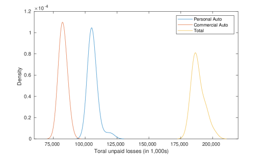
One advantage of the Bayesian methods employed in the aforementioned works is that they come equipped with a built-in uncertainty estimate for a single loss-reserve triangle. Calculating the variance of model parameters and confidence intervals is quite laborious in the CGMM. We instead opt to use the parametric bootstrap described in [Wüthrich and Merz, 2008]. To briefly summarize, we estimate the model parameters from the Schedule P data and generate new loss triangles from the results, re-estimating the parameters in this bootstrapped sample and outstanding claims. In Table 6.2, we can see the summary statistics from the bootstrapped samples, with the resulting outstanding claims reserve statistics in 6.3. We find that the results of Table 6.2 are similar to the celebrated chain ladder estimates for and . Given that the Tweedie is in some sense a parametric equivalent to these classic estimators, this is both unsurprising and also a validation of the CGMM estimates.
Table 6.1 summarizes our outstanding estimates alongside previous results using the same data set. There appear to be smaller variances in the CGMM results. A possible reason is the fact that in other methods relatively harsh uniform priors were used in a Bayesian framework; besides, the [Zhang and Dukic, 2013] results use heavier-tailed log-Normal marginals. In light of the simulation results in the previous section, we must also consider the possibility that the CGMM may be systematically underestimating the variance of outstanding claims.
| Personal | Commercial | Total | |||||||
| Model | Median | SD | Q(0.99) | Median | SD | Q(0.99) | Median | SD | Q(0.99) |
| Multivariate Tweedie (CGMM) | 104,935 | 3,750 | 121,377 | 82,038 | 2,052 | 87,715 | 187,542 | 4,786 | 201,928 |
| Multivariate Tweedie (Bayes) | 103,374 | 9,373 | 127,075 | 88,385 | 9,029 | 112,258 | 192,148 | 13,780 | 226,110 |
| Clayton Copula Tweedie (Bayes) | 103,674 | 18,742 | 166,187 | 91,067 | 15,820 | 135,924 | 194,741 | 28,376 | 283,931 |
| Gaussian Copula Tweedie (Bayes) | 107,930 | 21,502 | 172,161 | 92,773 | 17,902 | 147,734 | 200,703 | 31,333 | 295,900 |
| Personal Auto | Commercial Auto | |||||||||
| Median | SD | Q(0.05) | Q(0.95) | Median | SD | Q(0.05) | Q(0.95) | |||
| 0.2635 | 0.0071 | 0.2506 | 0.2706 | 0.1478 | 0.0142 | 0.1264 | 0.1675 | |||
| 0.2429 | 0.0067 | 0.2328 | 0.2512 | 0.1528 | 0.0107 | 0.1335 | 0.1653 | |||
| 0.2295 | 0.0058 | 0.2250 | 0.2430 | 0.1517 | 0.0148 | 0.1291 | 0.1687 | |||
| 0.2299 | 0.0082 | 0.2233 | 0.2516 | 0.1432 | 0.0180 | 0.1203 | 0.1731 | |||
| 0.2324 | 0.0062 | 0.2271 | 0.2457 | 0.1611 | 0.0200 | 0.1286 | 0.1830 | |||
| 0.2268 | 0.0108 | 0.2191 | 0.2424 | 0.1457 | 0.0138 | 0.1327 | 0.1797 | |||
| 0.2453 | 0.0042 | 0.2385 | 0.2527 | 0.1804 | 0.0105 | 0.1649 | 0.1919 | |||
| 0.2495 | 0.0042 | 0.2400 | 0.2526 | 0.1844 | 0.0084 | 0.1655 | 0.1930 | |||
| 0.2946 | 0.0068 | 0.2887 | 0.3008 | 0.1982 | 0.0054 | 0.1900 | 0.2033 | |||
| 0.2792 | 0.0018 | 0.2773 | 0.2815 | 0.2107 | 0.0025 | 0.2061 | 0.2140 | |||
| 1.0000 | 0.0000 | 1.0000 | 1.0000 | 1.0000 | 0.0000 | 1.0000 | 1.0000 | |||
| 0.9951 | 0.0044 | 0.9896 | 0.9999 | 0.9999 | 0.0023 | 0.9944 | 1.0000 | |||
| 0.5828 | 0.0045 | 0.5787 | 0.5883 | 0.8753 | 0.0036 | 0.8685 | 0.8770 | |||
| 0.3518 | 0.0100 | 0.3393 | 0.3691 | 0.7074 | 0.0044 | 0.7036 | 0.7220 | |||
| 0.1977 | 0.0139 | 0.1802 | 0.2194 | 0.4635 | 0.0075 | 0.4578 | 0.4744 | |||
| 0.0932 | 0.0100 | 0.0839 | 0.1089 | 0.1915 | 0.0111 | 0.1875 | 0.2135 | |||
| 0.0310 | 0.0038 | 0.0223 | 0.0333 | 0.1428 | 0.0045 | 0.1375 | 0.1481 | |||
| 0.0153 | 0.0045 | 0.0082 | 0.0224 | 0.0517 | 0.0048 | 0.0446 | 0.0567 | |||
| 0.0142 | 0.0043 | 0.0067 | 0.0197 | 0.0222 | 0.0026 | 0.0179 | 0.0250 | |||
| 0.0008 | 0.0193 | 0.0002 | 0.0715 | 0.0003 | 0.0018 | 0.0001 | 0.0010 | |||
| 0.0010 | 0.0001 | 0.0008 | 0.0011 | 0.0011 | 0.0001 | 0.0009 | 0.0013 | |||
| Systematic Parameters | ||||||||||
| 0.0073 | 0.0013 | 0.0054 | 0.0100 | |||||||
| 0.0027 | 0.0003 | 0.0023 | 0.0030 | |||||||
| Personal Auto | Commercial Auto | Total | ||||
|---|---|---|---|---|---|---|
| Accident Year | Mean | SD | Mean | SD | Mean | SD |
| 2 | 149.89 | 302.47 | 31.79 | 22.73 | 181.68 | 318.62 |
| 3 | 654.18 | 599.86 | 314.57 | 75.74 | 968.75 | 636.11 |
| 4 | 1,572.97 | 937.92 | 999.35 | 114.05 | 2,572.32 | 985.10 |
| 5 | 3,410.71 | 1,364.64 | 3,023.16 | 167.58 | 6,433.87 | 1,389.11 |
| 6 | 7,946.91 | 2,154.56 | 7,377.44 | 364.11 | 15,324.35 | 2,314.57 |
| 7 | 20,212.86 | 3,290.60 | 18,393.45 | 876.04 | 38,606.32 | 3,738.48 |
| 8 | 39,242.16 | 3,837.55 | 35,019.65 | 1,392.14 | 74,261.82 | 4,661.08 |
| 9 | 62,104.63 | 3,415.46 | 55,170.37 | 1,646.02 | 117,274.99 | 4,223.66 |
| 10 | 106,151.94 | 3,750.46 | 82,571.57 | 2,052.32 | 188,723.51 | 4,786.30 |
7 Conclusion
In this work, we have motivated the class of ABRMs with no closed-form PDF and proposed a novel application of the CGMM to estimate model parameters. Our methods are efficient and use moment generating functions alone. Though we primarily focus on Tweedie and Stable marginals in theory we are not limited to these distributions. We are also not bound by the form of ABRMs considered here. In the future, a more realistic model may incorporate separate scale parameters for each cell or multiple systematic components for a richer dependence structure.
We believe the results we have obtained in simulations and in an application to Schedule P data show promise for the CGMM in insurance applications. By constructing moment conditions that produce convex objective functions, we remove any need for overspecialized optimization packages or knowledge. Estimation remains generic and independent of the chosen model. That said, the art of solving ill-posed integral equations is challenging, and in the more complicated multi-LoB models further research is likely necessary.
Appendix A Distribution Background
A.1 Dispersion Models
Let and consider the Normal distribution function:
| (A.1) |
Notice that is a typical notion of distance. The Euclidian metric is a natural notion of distance over with which to describe errors; but how to extend it to , , , and so on? That is, we would like to make substitutions of form and that define new distributions such as
| (A.2) |
Bent Jørgensen used just this approach ([Jørgensen, 1987] and references therein) to create exponential dispersion models (EDMs). Naturally, will be proportional to the log-likelihood of the “” parameter (whatever that may represent). In this way, the theory of generalized linear models can be easily extended to non-Normal, non-Euclidean settings. It is not obvious, however, that for each there will be an appropriate normalization to produce a distribution. Put another way, given , can we find an that solves the following integral equation of the first kind:
| (A.3) |
In general, determining the existence and uniqueness of such a solution is hard and replete with technical issues (see Section 4.4). One strategy is to start with a solution and “invert” this to find the distribution. Consider a distribution with known cumulant function777Known as the partition function in physics and statistical mechanics. denoted by and defined as the logarithm of the MGF:
| (A.4) |
We can easily construct a distribution called the additive exponential dispersion model, given by ):
The transformation gives the reproductive exponential distribution model. Note that
| (A.6) |
and
| (A.7) |
implying that
The reproductive form of the pdf (given by ) is then
| (A.8) |
where is the negative log-likelihood888Assuming the range of is the same as the domain of ; otherwise we need to add terms. and . Having come full circle, we can regard as . Thus, maximizing likelihood is equivalent to minimizing the distance of some residual or error according to a metric determined by the partition function of the distribution – a highly elegant and useful construction! Note particularly that as long as we have a distribution and corresponding MGF we can construct a model of the kind in (A.5). Indeed, this is a very rich family of distributions found across the statistical sciences.
A.2 Tweedie Models
There is an interesting subclass of exponential dispersion models with useful properties and many well-known special cases. We begin by defining the unit variance function :
| (A.9) |
It can be shown that , uniquely determines the distribution. The Tweedie Exponential Dispersion models are characterized by the unit variance function , or equivalently as being the only EDMs closed under scale transforms. That is, if
then the EDM is Tweedie (denoted ). Notably, Tweedie models are also infinitely divisible (a concept discussed in the next appendix).
The parameter in the unit variance is called the Tweedie power parameter. Solving the ODE defining the Tweedie unit variance allows us to find the that generates the Tweedie models. Let ; then
| (A.10) |
Comparing this characterization to (A.6) and (A.7), we can easily recover a few common distributions:
-
•
is the Normal distribution,
-
•
is the Poisson distribution,
-
•
yields the Compound Poisson–Gamma distribution, and
-
•
is the Gamma distribution.
There are also some more exotic distributions: Inverse Gaussian () and some “extreme stable” distributions ( or ). It should be noted however that the latter distributions are only generated by Stable distributions and will only truly be Stable if .
Definition A.1 (Stable Random Variable, 1st definition).
A random variable is said to have a stable distribution if for , such that:
| (A.11) |
where the are independent copies of .
One can derive from this definition ([Zolotarev, 1986]) that the characteristic function for a stable variable is given by:
| (A.12) |
Denoted with . The and are the location and scale parameters, which are equal and proportional to the mean and variance, respectively, whenever they exist. Here is the tail parameter. For values of we have a Normal distribution, and for a Pareto tailed distribution with exponent . The value is a skewness parameter and if and support is either or . Finally, Stable random variables behave under addition operation much like the Normal. For and , then where:
| (A.13) | ||||
First appearing in Paul Lévy’s 1925 monograph Calcul des probabilités, Stable distributions went on to be studied by leading researchers, such as Andrey Kolmogorov and William Feller. One of the motivating problems of probability theory has been the distribution of sums of random variables. Stable random variables generalize the Normal as a basin of attraction to encompass all i.i.d. sums, not just the “nice” ones with finite variance or bounded support:
Theorem A.1.
(The generalized central limit theorem) Consider the sequence of centred and normalized sums of i.i.d RVs with Pareto tails such that:
and
Define:
and for 999In the normal case . See [Uchaikin and Zolotarev, 2011] for Cauchy case set:
and (if it exists, zero otherwise)
Then weakly where is a standardized stable distribution. i.e
While extremely useful, Stable distributions have historically been less popular than other models. This is likely due to the fact that Stable PDFs generally do not exist in closed form. There are however three notable cases where this is not true:
-
•
Normal ;
-
•
Cauchy (t with d.o.f=1) ;
-
•
Lévy .
Appendix B Misc tables
| DY | |||||||||||
|---|---|---|---|---|---|---|---|---|---|---|---|
| AY | Premium | 1 | 2 | 3 | 4 | 5 | 6 | 7 | 8 | 9 | 10 |
| 1 | 62467 | 16864 | 15508 | 9341 | 3537 | 1853 | 1184 | 500 | 308 | 338 | 50 |
| 2 | 59821 | 14528 | 17727 | 8747 | 4149 | 2252 | 715 | 325 | 261 | 255 | |
| 3 | 62968 | 14241 | 13763 | 7512 | 5207 | 2068 | 1674 | 219 | 421 | ||
| 4 | 64453 | 14765 | 14323 | 8426 | 6513 | 3144 | 1067 | 913 | |||
| 5 | 71185 | 16395 | 17038 | 9826 | 6381 | 4037 | 1839 | ||||
| 6 | 82793 | 18136 | 21582 | 13415 | 8519 | 4583 | |||||
| 7 | 100826 | 24727 | 24037 | 15181 | 7105 | ||||||
| 8 | 98358 | 24749 | 24501 | 11830 | |||||||
| 9 | 76653 | 23063 | 21035 | ||||||||
| 10 | 71326 | 20083 | |||||||||
| DY | |||||||||||
|---|---|---|---|---|---|---|---|---|---|---|---|
| AY | Premium | 1 | 2 | 3 | 4 | 5 | 6 | 7 | 8 | 9 | 10 |
| 1 | 42847 | 5407 | 9015 | 4641 | 3384 | 1695 | 1262 | 1425 | 373 | 241 | 6 |
| 2 | 38829 | 6279 | 8725 | 6172 | 4494 | 2110 | 919 | 447 | 202 | 69 | |
| 3 | 43001 | 7256 | 8667 | 4778 | 4262 | 2884 | 1427 | 889 | 493 | ||
| 4 | 41840 | 5028 | 5317 | 4697 | 3795 | 2871 | 1100 | 657 | |||
| 5 | 44525 | 5721 | 6097 | 6389 | 3802 | 4306 | 862 | ||||
| 6 | 50923 | 7413 | 9385 | 7772 | 5850 | 3383 | |||||
| 7 | 56601 | 10868 | 12337 | 7966 | 8531 | ||||||
| 8 | 54609 | 10143 | 14193 | 8070 | |||||||
| 9 | 47204 | 9596 | 12235 | ||||||||
| 10 | 42412 | 9076 | |||||||||
References
- [Ackerberg et al., 2014] Ackerberg, D., Chen, X., Hahn, J., and Liao, Z. (2014). Asymptotic efficiency of semiparametric two-step GMM. Review of Economic Studies, 81(3):919–943.
- [Alai et al., 2016] Alai, D. H., Landsman, Z., and Sherris, M. (2016). Multivariate Tweedie lifetimes: The impact of dependence. Scandinavian Actuarial Journal, 2016(8):692–712.
- [Asimit et al., 2010] Asimit, A. V., Furman, E., and Vernic, R. (2010). On a multivariate pareto distribution. Insurance: Mathematics and Economics, 46(2):308–316.
- [Asimit et al., 2016] Asimit, A. V., Vernic, R., and Zitikis, R. (2016). Background risk models and stepwise portfolio construction. Methodology and Computing in Applied Probability, 18:805–827.
- [Avanzi et al., 2016] Avanzi, B., Taylor, G., Vu, P. A., and Wong, B. (2016). Stochastic loss reserving with dependence: A flexible multivariate Tweedie approach. Insurance: Mathematics and Economics, 71:63–78.
- [Bee and Trapin, 2018] Bee, M. and Trapin, L. (2018). A characteristic function-based approach to approximate maximum likelihood estimation. Communications in Statistics: Theory and Methods, 47(13):3138–3160.
- [Carmean, 1995] Carmean, C. C. (1995). Environmental and asbestos liabilities: A growing concern for the insurance industry. Environmental Claims Journal, 8(1):131–140.
- [Carrasco et al., 2014] Carrasco, M., CIREQ, CIRANO, and Florens, J.-P. (2014). On the asymptotic efficiency of GMM. Econometric Theory, pages 372–406.
- [Carrasco and Florens, 2000] Carrasco, M. and Florens, J.-P. (2000). Generalization of GMM to a continuum of moment conditions. Econometric Theory, pages 797–834.
- [De Jong, 2012] De Jong, P. (2012). Modeling dependence between loss triangles. North American Actuarial Journal, 16(1):74–86.
- [Eaton et al., 1971] Eaton, M. L., Morris, C., and Rubin, H. (1971). On extreme stable laws and some applications. Journal of Applied Probability, 8(4):794–801.
- [Embrechts et al., 2013] Embrechts, P., Klüppelberg, C., and Mikosch, T. (2013). Modelling extremal events: For insurance and finance, volume 33. Springer Science & Business Media.
- [Fama and French, 2004] Fama, E. F. and French, K. R. (2004). The capital asset pricing model: Theory and evidence. Journal of economic perspectives, 18(3):25–46.
- [Feuerverger and McDunnough, 1981] Feuerverger, A. and McDunnough, P. (1981). On some Fourier methods for inference. Journal of the American Statistical Association, 76(374):379–387.
- [Fröhlich and Weng, 2018] Fröhlich, A. and Weng, A. (2018). Parameter uncertainty and reserve risk under Solvency II. Insurance: Mathematics and Economics, 81:130–141.
- [Furman et al., 2018] Furman, E., Kuznetsov, A., and Zitikis, R. (2018). Weighted risk capital allocations in the presence of systematic risk. Insurance: Mathematics and Economics, 79:75–81.
- [Furman et al., 2021] Furman, E., Kye, Y., and Su, J. (2021). Multiplicative background risk models: Setting a course for the idiosyncratic risk factors distributed phase-type. Insurance: Mathematics and Economics, 96:153–167.
- [Furman and Landsman, 2005] Furman, E. and Landsman, Z. (2005). Risk capital decomposition for a multivariate dependent gamma portfolio. Insurance: Mathematics and Economics, 37(3):635–649.
- [Furman and Landsman, 2010] Furman, E. and Landsman, Z. (2010). Multivariate Tweedie distributions and some related capital-at-risk analyses. Insurance: Mathematics and Economics, 46(2):351–361.
- [Hansen, 1982] Hansen, L. P. (1982). Large sample properties of generalized method of moments estimators. Econometrica: Journal of the Econometric Society, pages 1029–1054.
- [Jørgensen, 1987] Jørgensen, B. (1987). Exponential dispersion models. Journal of the Royal Statistical Society: Series B (Methodological), 49, (2):127–145.
- [Kotchoni, 2012] Kotchoni, R. (2012). Applications of the characteristic function-based continuum GMM in finance. Computational Statistics & Data Analysis, 56(11):3599–3622.
- [Koutrouvelis, 1980] Koutrouvelis, I. A. (1980). Regression-type estimation of the parameters of stable laws. Journal of the American Statistical Association, 75(372):918–928.
- [Mack, 1991] Mack, T. (1991). A simple parametric model for rating automobile insurance or estimating IBNR claims reserves. ASTIN Bulletin: The Journal of the IAA, 21(1):93–109.
- [Mack, 1993] Mack, T. (1993). Distribution-free calculation of the standard error of chain ladder reserve estimates. ASTIN Bulletin: The Journal of the IAA, 23(2):213–225.
- [Madigan and Metzner, 2003] Madigan, K. M. and Metzner, C. S. (2003). Reserving for asbestos liabilities. In CAS Forum, pages 173–212. Citeseer.
- [Marri and Moutanabbir, 2022] Marri, F. and Moutanabbir, K. (2022). Risk aggregation and capital allocation using a new generalized archimedean copula. Insurance: Mathematics and Economics, 102:75–90.
- [McAlea et al., 2016] McAlea, E. M., Mullins, M., Murphy, F., Tofail, S. A., and Carroll, A. G. (2016). Engineered nanomaterials: Risk perception, regulation and insurance. Journal of Risk Research, 19(4):444–460.
- [Merz et al., 2013] Merz, M., Wüthrich, M. V., and Hashorva, E. (2013). Dependence modelling in multivariate claims run-off triangles. Annals of Actuarial Science, 7(1):3–25.
- [Pai and Ravishanker, 2020] Pai, J. and Ravishanker, N. (2020). Livestock mortality catastrophe insurance using fatal shock process. Insurance: Mathematics and Economics, 90:58–65.
- [Ross, 2013] Ross, S. A. (2013). The arbitrage theory of capital asset pricing. In Handbook of the fundamentals of financial decision making: Part I, pages 11–30. World Scientific.
- [Samorodnitsky, 2017] Samorodnitsky, G. (2017). Stable non-Gaussian random processes: stochastic models with infinite variance. Routledge.
- [Seal, 1980] Seal, H. L. (1980). Survival probabilities based on Pareto claim distributions. ASTIN Bulletin: The Journal of the IAA, 11(1):61–71.
- [Semenikhine et al., 2018] Semenikhine, V., Furman, E., and Su, J. (2018). On a multiplicative multivariate gamma distribution with applications in insurance. Risks, 6(3):79.
- [Su and Furman, 2017a] Su, J. and Furman, E. (2017a). Multiple risk factor dependence structures: Copulas and related properties. Insurance: Mathematics and Economics, 74:109–121.
- [Su and Furman, 2017b] Su, J. and Furman, E. (2017b). Multiple risk factor dependence structures: Distributional properties. Insurance: Mathematics and Economics, 76:56–68.
- [Taylor, 2009] Taylor, G. (2009). Chain ladder for Tweedie distributed claims data. Variance, 3(1):96–104.
- [Uchaikin and Zolotarev, 2011] Uchaikin, V. V. and Zolotarev, V. M. (2011). Chance and stability: Stable distributions and their applications. Walter de Gruyter.
- [Wüthrich and Merz, 2008] Wüthrich, M. V. and Merz, M. (2008). Stochastic claims reserving methods in insurance, volume 435. John Wiley & Sons.
- [Zhang and Dukic, 2013] Zhang, Y. and Dukic, V. (2013). Predicting multivariate insurance loss payments under the Bayesian copula framework. Journal of Risk and Insurance, 80(4):891–919.
- [Zhou et al., 2018] Zhou, M., Dhaene, J., and Yao, J. (2018). An approximation method for risk aggregations and capital allocation rules based on additive risk factor models. Insurance: Mathematics and Economics, 79:92–100.
- [Zolotarev, 1986] Zolotarev, V. M. (1986). One-dimensional stable distributions, volume 65. American Mathematical Society.