Quantum imaginary time evolution and UD-MIS problem

Abstract

In this work we apply a procedure based on the quantum imaginary time evolution method to solve the unit-disk maximum independent set problem. Numerical simulations were performed for instances of 6, 8 and 10-qubits graphs. We have found that the failure probability of the procedure is relatively small and rapidly decreases with the number of shots. In addition, a theoretical upper bound for the failure probability of the procedure was obtained.

I Introduction

Obtaining the Hamiltonian ground state of a quantum system is of utmost importance for various physics problems and also for optimization problems. Quantum computing may be useful for calculating these states. Several quantum algorithms have been proposed for this purpose, including adiabatic quantum optimization [1], quantum annealing [2], and classical quantum variational algorithms such as the quantum approximate optimization algorithm (QAOA) [3] and the variational quantum eigensolver (VQE) [4, 5, 6]. Despite many advances, these algorithms also have potential drawbacks, especially in the context of near-term quantum computing architectures with limited quantum resources. For example, phase estimation is not practical without error correction, while variational quantum algorithms are limited in accuracy by a fixed ansatz and involve noisy high-dimensional classical optimizations [7].

Recently, a new approach to the quantum imaginary time evolution method (QITE) [8, 9, 10] has been proposed in [11]. This approach is based on emulating classical imaginary time evolution with measurement-assisted unitary circuits. However, unlike previous strategies, it is not a variational quantum algorithm. Some improvements of QITE algorithm have been developed for noisy intermediate-scale quantum (NISQ) hardware [12, 13, 14, 15]. QITE has found practical application in quantum chemistry on NISQ hardware [16, 17], in simulating open quantum systems [18], and recently in optimization problems such as Max-Cut and polynomial unconstrained boolean optimization (PUBO) [19, 20]. QITE seems to have an advantage over QAOA [3, 21, 22, 23, 24, 25, 26] since there is no need for classical optimization parameters, distinguishing from it. Furthermore, it does not employ ancilla qubits like VQE [5, 6].

The MaxCut and the Maximum Independent Set problems are prototypical examples of optimization problems that have received attention as candidates for quantum advantage [27, 28, 29, 30, 31, 32, 33, 34, 35, 36, 37]. The unit-disk maximum set problem (UD-MIS) is computationally challenging. It belongs to the class of NP-hard problems, which means that finding an exact solution efficiently for large instances is infeasible. Studies using quantum hardware an algorithms to tackle UD-MIS problems are being conducted [38, 39, 40, 29]. For instance, in [40] quantitative requirements on system sizes and noise levels of Rydberg atoms platforms were studied to reach quantum advantage in solving UD-MIS with a quantum annealing-based algorithm. In [29] it was compared the probability for finding the UD-MIS solution using an analog quantum annealing algorithm to the QAOA algorithm with no quantum noise.

In this work we will apply a procedure based on QITE algorithm proposed in [11] to solve UD-MIS problems. We will simulate, without noise, QITE with two non-trivial domains and apply it to several UD-MIS instances of 6, 8 and 10 qubits. We will explore the number of iterations and shots required for our probabilistic procedure to return acceptable results.

The paper is organized as follows. In section II we review the quantum imaginary-time evolution method presented in [11]. We provide some notations and definitions that will be useful later on. In Section III we describe our proposed method for solving optimization problems using QITE. In Section IV we briefly describe the UD-MIS problem and we explain how this problem can be formulated in terms of the Hamiltonian of a quantum system. In Section V we test numerically the proposed method on several intances of UD-MIS problems. In Section VI, we give some concluding remarks. For readability, auxiliary lemmas and proofs, and an explanation of numerical calculations are presented separately in Appendices A and B, respectively.

II Quantum imaginary-time evolution method

In this section we review the imaginary-time evolution (ITE) method and a quantum proposal for it [11]. The imaginary-time evolution method is a well-known approach used for obtaining the ground state of a quantum Hamiltonian. The idea is to express the ground-state $\ket{\psi}$ of the Hamiltonian as the long-time limit of the imaginary-time Schrödinger equation, that is,

$$\ket{\psi}=\lim_{t\rightarrow\infty}\ket{\psi^{ite}_{t}},~{}~{}~{}\ket{\psi^{ite}_{t}}=\frac{e^{-tH}\ket{\psi_{0}}}{||e^{-tH}\ket{\psi_{0}}||},$$ (1)

for some initial state $|\psi_{0}\rangle$, with the condition $\langle\psi_{0}|\psi\rangle\neq 0$. The parameter $t$ must be chosen such that the final state is close enough to the ground state. This parameter can also be thought of as the inverse temperature ($t=\frac{1}{k_{B}T}$, where $k_{B}$ is the Boltzmann constant and $T$ is the temperature). In this case, Eq. (1) states that the system tends to the ground state when temperature tends to zero.

In [11] it was proposed a quantum imaginary-time evolution method (QITE) that emulates Eq. (1). It consists of measurement-assisted unitary circuits, acting on suitable domains around the support of different qubits. To be more precise, start with a geometric $k$-local Hamiltonian with $m$ terms of the form:

$$H=\sum^{m}_{l=1}h[l].$$ (2)

Each term $h[l]$ acts on at most $k$ (neighboring) qubits on an underlying graph. Let us consider a Trotter decomposition of the corresponding imaginary time evolution

$$e^{-tH}=(e^{-\tau h[1]}e^{-\tau h[2]}\cdots e^{-\tau h[m]})^{n}+\mathcal{O}(\tau^{2}),~{}~{}~{}\tau=t/n,$$ (3)

acting on an initial state $\ket{\psi_{0}}$ (usually taken to be a product state). In the decomposition we have $n$ iteration of the form $e^{-\tau h[1]}e^{-\tau h[2]}\cdots e^{-\tau h[m]}$, and each $e^{-\tau h[l]}$ is a sub-step of a complete iteration step. The interval $\tau$ must be chosen such that the squared errors are negligible.

After a Trotter sub-step $e^{-\tau h[l]}$ of the iteration $j$ we have

$$|\psi^{\prime}\rangle=\frac{e^{-\tau h[l]}}{||e^{-\tau h[l]}|\psi\rangle||}|\psi\rangle.$$ (4)

The idea is to map the scaled non-unitary action $e^{-\tau h[l]}$ of the iteration $j$ on the state $\ket{\psi}$ to that of a unitary evolution $e^{-i\tau A[l,j]}$:

$$|\psi^{\prime}\rangle\approx e^{-i\tau A[l,j]}|\psi\rangle.$$ (5)

Here $A[l,j]$ is a Hermitian operator associated to the $l$-th term $h[l]$ of iteration $j$ acting on a qubit domain $D_{l,j}$ of dimension $d_{l,j}$. The domain is usually chosen around the support of $h[l]$. $A[l,j]$ can be expanded as a sum of Pauli strings acting on $D_{l,j}$,

$$A[l,j]=\sum_{I}a[l,j]_{I}\sigma_{I},~{}~{}I=i_{1}i_{2}\ldots i_{d_{l,j}},$$ (6)

with $\sigma_{I}=\sigma_{i_{1}}\otimes\cdots\otimes\sigma_{i_{d_{l,j}}}$, and $\sigma_{i_{k}}$ being a Pauli matrix with $i_{k}\in\{I,X,Y,Z\}$, and it is understood that identity matrices should be inserted in the product when appropriately.

The goal is to minimize the difference $||\ket{\psi^{\prime}}-(1-i\tau A[l,j])\ket{\psi}||^{2}$ with respect to real variations of $a[l,j]_{I}$, where $||\cdot||$ is the norm of the Hilbert space. Up to $\mathcal{O}(\tau^{2})$ errors, this difference translates into a linear problem in the coefficients $a[l,j]_{I}$:

$$\sum_{J}(S+S^{T})_{IJ}a_{J}[l,j]=-b_{I},$$ (7)

where $S_{IJ}=\langle\psi|\sigma_{I}\sigma_{J}|\psi\rangle$ and $b_{I}=-2\mbox{Im}\langle\psi|\sigma_{I}h[l]|\psi\rangle$. In order to obtain $S_{IJ}$ and $b_{I}$, we need to perform suitable measurements of the state $|\psi\rangle$. Solving the linear equation (7), we obtain the coefficients $a[l,j]$. From $a[l,j]$ we obtain the unitary evolution $e^{-i\tau A[l,j]}$ for the corresponding sub-step. Finally, iterating this process for the $m$ terms of the Hamiltonian and the $n$ iteration steps, we construct the QITE operator:

$$\mbox{Q}_{H}(\tau,n,\mathcal{D})=\prod_{j=1}^{n}\prod_{l=1}^{m}e^{-i\tau A[l,n+1-j]}.$$ (8)

Here $\mathcal{D}$ contains the information of all domains $D_{l,j}$, with $1\leq l\leq n$ and $1\leq j\leq m$. Finally, the QITE evolution is given by

$$|\psi_{0}\rangle\rightarrow\ket{\phi^{qite}_{t}}=\mbox{Q}_{H}(\tau,n,\mathcal{D})|\psi_{0}\rangle.$$ (9)

For simplicity, in the Section V we will fix all domains to be equal on each step (but not on each sub-step), that is, for each $1\leq l\leq m$, $D_{l,1}=\cdots=D_{l,n}$.

In the construction of the QITE operator we have to define for each sub-step the domain of qubits where the Pauli strings act. In [11] it is argued that as the sub-steps increase, the dimension of the domain should increase from an initial domain that involves the qubits associated to the natural support of each $h[l]$. In general, this is due to an expected increase in correlations between qubits when starting from a product state. However, it is argued that for systems with finite correlations over at most $C$ qubits bounded by $\mbox{exp}(-L/C)$, with $L$ the distance between the observables, the domain can be chosen with a width of at most $\mathcal{O}(C^{D})$ surrounding the qubits on the support of $h[l]$ ($D$ the dimension of the underlying regular lattice). They also argue that the number of measurements and classical storage at a given time step required to perform the QITE computation is bounded by $\mbox{exp}(\mathcal{O}(C^{D}))$, but it scales in a quasi-polynomial way in terms of the numbers of qubits. In practice, however, we can choose a fixed domain smaller than the one induced by $C$ by truncating the unitary updates on each step to domain dimensions that fit the computational budget. Of course, the larger the dimension the better the approximation to the ground-state. Nevertheless, this approximate QITE version remains useful as a valid heuristic. We will use this approximate version all along this work.

III Optimization method based on QITE

Let us consider a quantum system of $N$ qubits, with Hilbert space $\mathcal{H}=\mathbb{C}^{2}\otimes\cdots\otimes\mathbb{C}^{2}$, and dimension $d=2^{N}$. We consider a diagonal Hamiltonian in the computational basis $\{|i\rangle\}_{0\leq i\leq d-1}$, given by

$$H=aI+\sum_{i=0}^{N-1}b_{i}Z_{i}+\sum_{(i,i^{\prime})}^{N-1}c_{i,i^{\prime}}Z_{i}Z_{i^{\prime}},$$ (10)

with $I$ the identity operator, $Z_{i}$ the $Z$ Pauli matrix acting on the i-th qubit, and $a$, $b_{i}$, $c_{i,i^{\prime}}$ real coefficients. We denote $E_{0},\ldots,E_{d-1}$ the eigenvalues of the Hamiltonian $H$, with all the $E_{i}$ sorted in an non-decreasing way (each eigenvalue has to be considered with their respective degeneracy). We denote the corresponding eigenstates respectively as $|E_{0}\rangle,\ldots,|E_{d-1}\rangle$, where some $|E_{i}\rangle$ should be understood as belonging to the same eigenspace. Since the Hamiltonians are diagonals in the computational basis, that is, the eigenvectors of $H$ are the vectors of the computational basis, the basis $\{|E_{i}\rangle\}_{0\leq i\leq d-1}$ can be chosen such that it has the same elements of the computational basis, but in different order. In this work, the basis $\{|E_{i}\rangle\}_{0\leq i\leq d-1}$ is chosen in such a way.

The problem we want to solve is the following: Finding the lowest eigenvalue $E_{0}$ of $H$ or an eigenvalue $E_{i}$ such that $E_{i}\leq E_{0}+\delta E$, with $\delta E\geq 0$ a tolerable error.

In order to solve this problem, we propose the following probabilistic method (see Alg.1) based on QITE:

1. We start with an initial state $|\psi_{0}\rangle=\mathbf{H}^{\otimes N}|0\ldots 0\rangle$, where $\mathbf{H}^{\otimes N}$ is the Hadamard gate acting on each qubit. In terms of the eigenvectors basis of $H$, the initial state has the form $\ket{\psi_{0}}=\frac{1}{\sqrt{d}}\sum_{i=0}^{d-1}\ket{E_{i}}$.

2. Then, we apply the QITE operator up to a time $t_{max}$:

   $$|\psi_{0}\rangle\rightarrow\ket{\phi^{qite}_{t_{max}}}=\mbox{Q}_{H}(\tau,n_{max},\mathcal{D})|\psi_{0}\rangle,$$ (11)

   where $t_{max}$, $\tau$, and $\mathcal{D}$ should be chosen according to the particular problem, and $n_{max}=t_{max}/\tau$.

3. We measure $|\phi^{qite}_{t}\rangle$ $M$ times ($M$ number of shots) in the computational basis, with $M<<d$. We register the $M$ outputs $E_{i_{m}}$, with $1\leq m\leq M$.

4. Finally, with a classical computer, we choose from the $M$ outputs $E_{i_{m}}$ the one with less energy.

The general idea of the method is the following. When applying QITE operator $\mbox{Q}_{H}(\tau,n_{max},\mathcal{D})$ to the initial state $\ket{\psi_{0}}$, as $n_{max}$ grows, it is expected to obtain a superposition of eigenstates of $H$ with higher probabilities for the eigenstates with the smallest eigenvalues. In the case of Hamiltonians of the form given in Eq. (10), the Hamiltonian basis coincides with the computational basis. Therefore, when measuring in the computational basis, we obtain eigenstates of $H$, and we expect to obtain with more probability the eigenstates with lower eigenvalues. If we consider $M$ shots, the more we increase $M$, the more likely we are to get a good result, that is, a state with eigenvalue $E_{i}$ such that $E_{i}\leq E_{0}+\delta E$ with $\delta E$ a tolerable error. However, the number of shots should not increase exponentially with the number of qubits, otherwise in the fourth step of the procedure we end up in a $for$ loop with an exponential number of iterations. In Section V we will numerically show that an exponential increase in $M$ is not needed.

It should be noted that the state obtained by our method and the QITE state $|\phi^{qite}_{t}\rangle$ are not necessarily the same. While the first one is an eigenstate of $H$, obtained after a measurement, the second one, in general, is a superposition of eigenstates. When this output state is such that $E_{i}\leq E_{0}+\delta E$ with $\delta E$ a tolerable error, we will call it an acceptable state.

Since the proposed method is probabilistic, there is a failure probability associated with it, and the lower it is, the higher the chances of obtaining at least one acceptable eigenvalue of $H$ after $M$ shots. Given the QITE state at time $t$, $\ket{\phi^{qite}_{t}}$, when measuring one time ($M=1$) in the computational basis, the failure probability is the probability of obtaining an eigenvalue $E_{i}>E_{0}+\delta E$, which is given by

$$P_{F}^{qite}(t)=\sum_{E_{i}>E_{0}+\delta E}|\langle E_{i}\ket{\phi^{qite}_{t}}|^{2}.$$ (12)

When measuring $M$ times in the computational basis, the failure probability for the QITE state at time $t$ is $(P_{F}^{qite}(t))^{M}$.

In the ideal case, the QITE state at time $t$, $\ket{\phi^{qite}_{t}}$, coincides with the ITE state at time $t$, $\ket{\psi^{ite}_{t}}$, given by Eq. (1). The ITE state sometimes will be called exact state in Section V. It can be expressed in terms of the eigenvectors of the Hamiltonian as follows:

$$\ket{\psi^{ite}_{t}}=\frac{1}{\mathcal{K}}\sum_{i=0}^{d-1}e^{-tE_{i}}|E_{i}\rangle,~{}~{}~{}\mbox{with}~{}~{}~{}\mathcal{K}^{2}=\sum_{i=0}^{d-1}e^{-2tE_{i}}.$$ (13)

We can compute the failure probability for the ITE state:

$$P_{F}^{ite}(t)=\sum_{E_{i}>E_{0}+\delta E}|\langle E_{i}\ket{\psi^{ite}_{t}}|^{2}=\sum_{E_{i}>E_{0}+\delta E}\frac{e^{-2tE_{i}}}{\mathcal{K}^{2}}.$$ (14)

We are interested in an upper bound for the failure probability independent of the Hamiltonian $H$. The following theorem provides a relevant bound for the ITE failure probability.

Theorem 1 (ITE failure probability upper bound).

Let $H=\sum_{i=0}^{d-1}E_{i}\ket{E_{i}}\bra{E_{i}}$ be a Hamiltonian of a quantum system with the fundamental eigenvalue with degeneracy $g$, and $\delta E\geq 0$ a tolerance. The failure probability for $\ket{\psi^{ite}_{t}}$ satisfies the inequality

$$P_{F}^{ite}(t)\leq\frac{1}{1+g(d-g)^{-1}e^{2t\delta E}}.$$ (15)

From this result we can obtain useful relations between the parameters of the proposed method. Eq. (15) can be restated as $P_{F}^{ite}(t)\leq 1/(1+ge^{2t\delta E-N\ln{2}})$. When measuring $M$ times, this expression has an exponent $M$. Then, it is enough that the parameters satisfy $2t\delta E\gtrapprox N\ln{2}$ in order to obtain a good upper bound. This implies that time need not increase more than linearly with the number of qubits.

The ITE upper bound can be connected with the QITE upper bound. The following theorem provides a relation between the ITE failure probability and the QITE failure probability.

Theorem 2 (QITE failure probability upper bound).

Let $H=\sum_{i=0}^{d-1}E_{i}\ket{E_{i}}\bra{E_{i}}$ be a Hamiltonian of a quantum system, $\delta E\geq 0$ a tolerance, and $\ket{\psi^{ite}_{t}}$ and $\ket{\phi^{qite}_{t}}$ the corresponding ITE and QITE states at time $t$. Given $0\leq\varepsilon\leq\sqrt{2}$, if $||\ket{\psi^{ite}_{t}}-\ket{\phi^{qite}_{t}}||\leq\varepsilon$, the failure probabilities $P_{F}^{ite}(t)$ and $P_{F}^{qite}(t)$ satisfy

$$|P_{F}^{qite}(t)-P_{F}^{ite}(t)|\leq\varepsilon\sqrt{1-\frac{\varepsilon^{2}}{4}}.$$ (16)

Thm. 2 shows how the QITE failure probability is related with distance between QITE and ITE states. Motivated by this theorem we define the following quantities that will be analyzed later on:

$$\varepsilon(t)=||\ket{\psi^{ite}_{t}}-\ket{\phi^{qite}_{t}}||,$$ (17)

$$\bar{\varepsilon}(t)=||\ket{\psi^{ite}_{t_{max}}}-\ket{\chi_{t}}||,$$ (18)

where $\ket{\chi_{t}}$ could be either $\ket{\psi^{ite}_{t}}$ or $\ket{\phi^{qite}_{t}}$. The quantity $\varepsilon(t)$ tells us how much departs the QITE state from the ITE state at time $t$, and $\bar{\varepsilon}(t)$ tells how much the corresponding state at time $t$ departs from the ITE state at a final time $t_{max}$. For an iterative process, $\bar{\varepsilon}(t)$ shows how well $\ket{\chi_{t}}$ is approximating the expected solution $\ket{\psi^{ite}_{t_{max}}}$ at a certain iteration step.

$|\phi_{0}\rangle\leftarrow\mathbf{H}^{\otimes n}|0\ldots 0\rangle$ $\triangleright$ Initial state

$t\leftarrow t_{max}$$\triangleright$ $t_{max}=\tau\times n_{max}$, with $n_{max}$ iterations.

$H\leftarrow\mbox{Optimization Hamiltonian}$

$|\phi^{qite}_{t_{max}}\rangle\leftarrow\mbox{Q}_{H}(\tau,n_{max},\mathcal{D})|\phi_{0}\rangle$

$\mbox{Measure }|\phi^{qite}_{t_{max}}\rangle~{}M\mbox{ times}~{}(\mbox{computational basis}).~{}~{}\mbox{Keep each measured state:}~{}~{}|E_{i_{m}}\rangle,~{}~{}1\leq m\leq M.$$\triangleright$ $M$: Number of shots

for $m\leq M$ do

     $E_{i_{m}}\leftarrow\langle E_{i_{m}}|H|E_{i_{m}}\rangle$

     $m\leftarrow m+1$

end for

return $|E_{i_{m}}\rangle~{}\mbox{associated with lowest}~{}E_{i_{m}},~{}1\leq m\leq M.$

Algorithm 1

IV Unit-disk maximum independent set problem

In this section, we describe the unit-disk maximum independent set problem (UD-MIS), a basic graph optimization problem with many applications. We also explain how this problem can be formulated in terms of the Hamiltonian of a quantum system.

Let $G=(V,E)$ be a graph with vertex set $V$ and edge set $E$, and let $N$ be the number of vertices of the graph $G$. An independent set of $G$ is a set of mutually non-connected vertices. Let $S=(s_{1},\ldots,s_{N})$ be a bitstring of length $N$ ($s_{i}\in\{0,1\}$), and let $\mathcal{B}_{N}$ be the set of all possible bitstrings of length $N$. The size of $\mathcal{B}_{N}$ is exponential in the graph size, $|\mathcal{B}|=2^{N}$. The Hamming weight of a bitstring $S$ is given by $|S|=\sum_{i=1}^{N}s_{i}$. The maximum independent set (MIS) problem consists in determining the size of the largest possible independent set and returning an example of such a set. This problem can be formulated as the following maximization problem:

$$\max_{S\in\mathcal{B}} |S|$$ (19)

s.t. $$S\in I.S,$$

where $I.S$ (for “Independent Sets”) is the set of bitstrings $(s_{1},\ldots,s_{N})$ corresponding to independent sets of $G$. A bitstring $S=(s_{1},\ldots,s_{N})$ corresponds to an independent set if for all pair of vertices $(i,i^{\prime})$ we have $s_{i}=s_{i^{\prime}}=1\implies(i,i^{\prime})\notin E$.

The UD-MIS problem is the MIS problem restricted to unit-disk graphs. A graph is a unit-disk graph if one can associate a position in the 2D plane to every vertex such that two vertices share an edge if and only if their distance is smaller than unity.

This optimization problem can be reformulated as a quantum minimization problem that consists in finding the ground state of a Hamiltonian of a quantum system. The idea is to associate to each bitstring $S=(s_{1},\ldots,s_{N})$ a quantum state $|s_{1},\ldots,s_{N}\rangle$ of the $N$-qubit system. The associated Hamiltonian is the following:

$$H=-\sum_{i\in V}\hat{n}_{i}+u\sum_{(i,i^{\prime})\in E}\hat{n}_{i}\hat{n}_{i^{\prime}},$$ (20)

with $\hat{n}_{i}=(I-Z_{i}$)/2 and $Z_{i}$ the Pauli matrix in the $z$ direction acting on the qubit $i$, and $u$ a parameter whose value can be adjusted. Fixing $u>1$ guarantees that the ground state of $H$ will necessarily be an independent set.

The Maximum Independent Set problem, along with the MaxCut problem, are prototypical examples that have received attention as candidates for quantum advantage [27, 28, 29, 30, 31, 32, 33, 34, 35, 36, 37, 40] The unit-disk maximum set problem is computationally challenging. It belongs to the class of NP-hard problems, which means that finding an exact solution efficiently for large instances is infeasible and that any NP optimization problem can be reformulated as a UD-MIS problem with polynomial overhead [41]. Researchers have developed several heuristic algorithms to approximate this problem. The are two main strategies that can be distinguished. One base on 2-level shifting schemes [42, 43, 44, 45] and the other based on breadth-first-search schemes [46].

Here, we are going to solve it applying the optimization method based on QITE described in Section III. It should be noted that the Hamiltonian given in (20) does not depend on the actual distances of the nodes, but the links between them. This implies that correlations between nodes are affected by the links they share rather than the geometric distance between them. The QITE method is expected to work well under the assumption of finite correlation length with a geometric k-local Hamiltonian [11]. The UD-MIS graphs do not have, in general, a regular lattice shape as can be seen in Fig. 1. This means that correlation lengths may not follow an exponential decaying law between node distances in the graph. Regardless of this, we have used QITE as a valid heuristic method.

V Numerical results

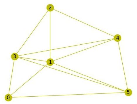
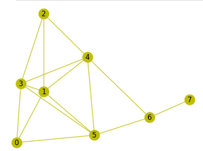
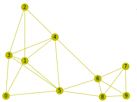
Figure 1: Examples of UD-MIS graphs consisting of 6 (a), 8 (b) and 10 (c) qubits.

In this section we apply the optimization method based on QITE (Alg. 1) described in Section III, to solve the UD-MIS problem presented in Section IV. In this section we summarize our numerical findings. We first explore several numerical quantities and analyze the failure probability for graphs of Fig. 1. Then, we test the method by sampling several random graphs. We use Hamiltonians of the form given in Eq. (20) with $u=1.35$.

V.1 Failure probability characterization

We recall from section III that the aim of our method is to obtain an acceptable state, that is, an eigenstate with eigenvalue $E_{i}$ such that $E_{i}\leq E_{0}+\delta E$, with $\delta E\geq 0$ a tolerable error. In what follows, we numerically explore several quantities for the graphs instances depicted in Fig. 1 in order to understand how the performance of the method relates to the number of iterations, the domains, and the number of shots. The Hamiltonian for these graphs are constructed according to Eq. (20). The results will be used later on when testing Alg. 1 on several instances of random graphs.

In an ideal case, that is when we choose a full domain $\mathcal{D}$ and a very small interval $\tau$, the QITE state at time $t$, $\ket{\phi^{qite}_{t}}$, should approximate very well the ITE state at time $t$, $\ket{\psi^{ite}_{t}}$. In practical cases the matching between these two states would depend on the chosen domain and the number of iterations. The difference between them can be characterize by $\varepsilon(t)$, given in Eq. (18), or by the fidelity. The closer the QITE state is to the ITE state, the closer the QITE failure probability $P_{F}^{qite}(t)$ is to the ITE failure probability $P_{F}^{ite}(t)$, and the better the results of our algorithm should be. Thm. 2 gives an upper bound for the difference between QITE and ITE failure probabilities in terms of $\varepsilon(t)$. We thus start plotting $\varepsilon(t)$ and $\bar{\varepsilon}(t)$ (Eq. (17) and (18), respectively) for the 6-qubit graph instance of Fig. 1a. In all numerical simulations we have set $\tau=0.01$, so $t_{max}$ is fixed with the number of iterations, $n_{max}$. For the 6-qubit graph instance we have used $t_{max}=10$ (i.e. $n_{max}=1000$). We have chosen two different domains: $\mathcal{D}_{A}$ and $\mathcal{D}_{B}$. $\mathcal{D}_{A}$ is chosen in such a way that each $D_{l,j}$ equals the same qubit support of $h[l]$ for all iterations $1\leq j\leq n_{max}$. $\mathcal{D}_{B}$ is chosen in a similar way to $\mathcal{D}_{A}$ except that associated domains with terms containing $Z_{i}Z_{i^{\prime}}$ are expanded to contain a 4-qubit support around the linked qubits $i$ and $i^{\prime}$ (see Appendix B for details). It should be noted that these domains imply that the evolution given by Eq. (11) produces entanglement between qubits. This differs from other proposals where QITE is applied with a linear ansatz [19, 20].

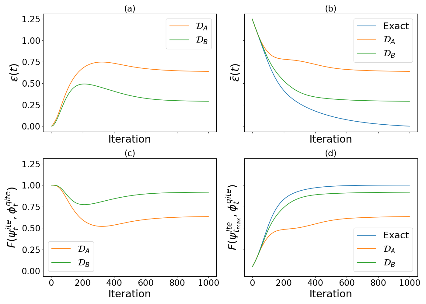
Figure 2: Error and fidelity results for the 6-qubit graph instance of Fig. 1a for different domains. (a) and (c) depict plots of $\varepsilon(t)$ (Eq. (17)) and $F(\psi^{ite}_{t},\phi^{qite}_{t})=|\langle\psi^{ite}_{t}|\phi^{qite}_{t}\rangle|^{2}$, respectively. (b) and (d) depict plots of $\bar{\varepsilon}(t)$ and fidelity $F(\psi^{ite}_{t_{max}},\phi^{qite}_{t})=|\langle\psi^{ite}_{t_{max}}|\phi^{qite}_{t}\rangle|^{2}$. The blue line corresponds to calculate the fidelity with respect to the ITE state $|\psi^{ite}_{t}\rangle$.

In Fig. 2a and 2b we plot $\varepsilon(t)$ and $\bar{\varepsilon}(t)$. Fig 2a shows that $\ket{\psi^{ite}_{t}}$ and $\ket{\phi^{qite}_{t}}$ start to depart from each other as the number iterations increases, reaching a plateau for long iterations. Lower values of $\varepsilon(t)$ indicate a good fit between both states while higher values show the contrary. If both states are almost orthogonal, this implies that $\varepsilon(t)$ is near to $\sqrt{2}$. It should be noted that for all iterations we have $\varepsilon(t)\leq\sqrt{2}$, satisfying hypothesis of Thm. 2. For a better comparison, we have plotted the fidelity between both states in Fig. 2c. Fig. 2d shows convergence of QITE state to $|\psi^{ite}_{t_{max}}\rangle$ as the domain dimension and the number of iterations increase. Regarding the chosen domains, we find that $\mathcal{D}_{B}$ performs better than $\mathcal{D}_{A}$ as expected, since $\mathcal{D}_{B}$ has a bigger domain than $\mathcal{D}_{A}$. However, this comes at the cost of needing more expectation values to obtain coefficients $a_{I}[l,j]$, and bigger linear systems to solve. From these plots we see that the low-dimensional domain $\mathcal{D}_{A}$ does not perform very well compared to $\mathcal{D}_{B}$ in matching the ITE state for large number of iterations. However, as we said in Section III, we are interested in using QITE to get a state with eigenvalue $E_{i}$ such that $E_{i}\leq E_{0}+\delta E$, with $\delta E$ a tolerable error. Moreover, we are interested in low-dimensional domains to ensure few measurements of expectation values (less coefficients $a[l,j]$ to be computed) and in few iterations to avoid deep quantum circuits. For this, we analyze in Fig. 3 and Fig. 4 how $P_{F}^{qite}(t)$ behaves as $t$ increases together with the number of shots $M$.

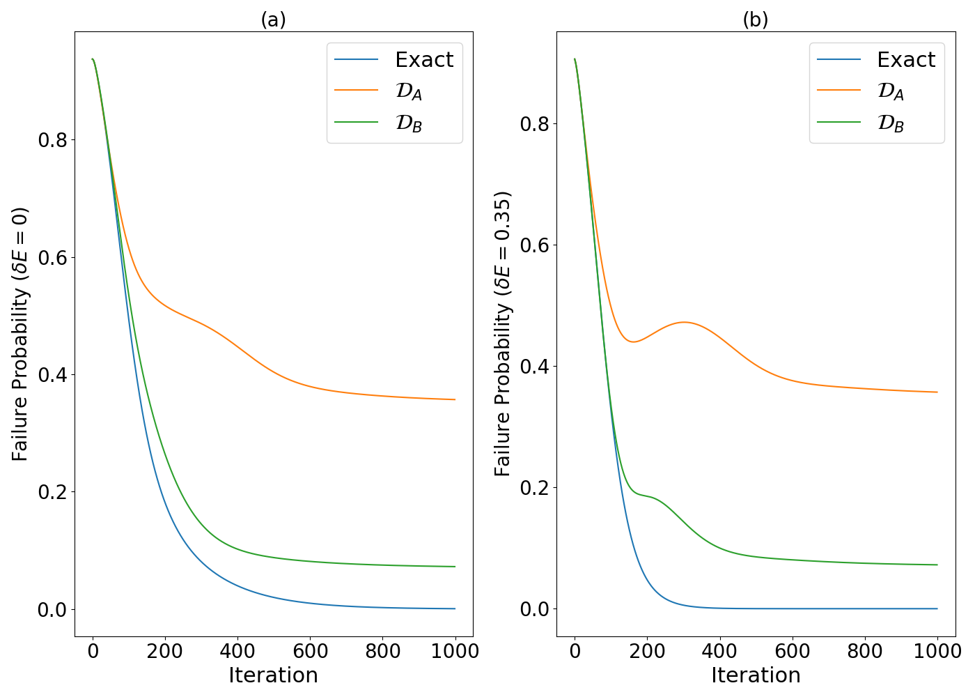
Figure 3: Failure probability for 6-qubit graph (Fig 1a). (a) $P_{F}^{ite}(t)$ (blue line) and $P_{F}^{qite}(t)$ for different domains and $\delta E=0$. (b) Similar to (a) but $\delta E=0.35$. This value represents the difference between the energy ground-state $E_{0}=-2$ and the energy of the first excited state $E_{1}=-1.65$. The degeneracy of the ground states is $g=3$ and for first excited states is $g=2$.

Figure 4: Failure probability $(P_{F}^{qite}(t))^{M}$ vs $M$ (number of shots) for 6-qubit graph for different number of iterations and domains.

In Fig. 3 we see that $P_{F}^{qite}(t)$ decreases a $t$ grows. Also, we see that $\mathcal{D}_{B}$ seems to be a much better option than $\mathcal{D}_{A}$ for getting low values of $P_{F}^{qite}(t)$. However, as stated before, even using $\mathcal{D}_{A}$ and a low number of iterations we might get good results, since we are only interested in getting acceptable states. This is what we see in Fig. 4 when the number of shots is taking into account. $(P_{F}^{qite}(t))^{M}$ decreases considerable as the number of shots increases for different domains and number of iterations. In both Fig. 3 and 4, $\delta E$ has been chosen to include not only the ground state but also first-excited states as acceptable states (since the energy gap is roughly around $0.35$, then $\delta E=0.35$). For this 6-qubit graph instance, $\delta E$ represents 17.5% of the ground state energy (see description of Fig. 3b). This implies that we are tolerating relative errors up to 17.5%. The relative error is computed as $100\times|E_{0}-E_{i}|/|E_{0}|$, with $E_{i}$ the obtained eigenvalue and $E_{0}$ the ground state energy. Fig. 4 shows, for different domains, how many iterations and number of shots are needed to get a reasonable low probability of failure for our method. It should be noted that the number of shots can be kept to be proportional to the number of qubits to obtain good results.

We have also repeated the same analysis for the 8 and 10-qubit graphs. These cases have a similar behaviour compared to the 6-qubit graph (see Appendix B.1 and B.2 for numerical results). Based on these results, for our purposes it will be sufficient to test Alg. 1 on randomly generated instances using $\mathcal{D}_{A}$ with $100$ iterations and $M$ at most equal to $2N$ ($N$ number of qubits). This is what we do in the next subsection.

V.2 Testing random samples of UD-MIS graphs

Based on the analysis of previous subsection we have tested Alg. 1 on several random UD-MIS graphs for $6$, $8$ and $10$ qubits with domain $\mathcal{D}_{A}$, $n_{max}=100$ iterations and $\tau=0.01$. We tested on approximately $400$ graphs for $6$ qubits, $150$ graphs for $8$ qubits and $10$ graphs for $10$ qubits.

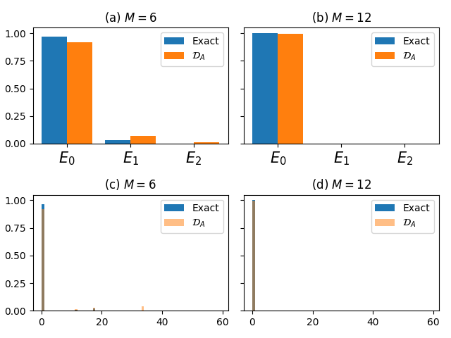
Figure 5: (a) and (b) show normalized histograms of obtained eigenvalues for 6-qubit graphs, with number of shots $M=6$ and $M=12$, respectively. (c) and (d) show normalized histograms of relative errors for $M=6$ and $M=12$ shots. The number of UD-MIS instances to make these plots was around 400.

In Fig. 5a and 5b we plotted, for $M=6$ and $M=12$ shots, the normalized histogram of obtained eigenvalues using Alg. 1 for 6-qubits graphs. In Fig. 5c and 5d we plotted, the histogram of relative errors. From Fig. 5a we conclude that even for $M=6$ shots the Alg. 1 returns acceptable results, in accordance with Fig. 4. For this random sample of 6-qubits graphs, the energy gap is roughly around $0.35$, representing at least a $15\%$ of the ground state. When the gap is small, it is more difficult to find the ground state, since there is a greater probability of obtaining lower-energy excited states. However, in this case, the relative error is small. Therefore, from an optimization point of view, all these states are expected to be acceptable states since the difference in the cost function is very small.

We have also sampled random graphs for $8$ and $10$-qubits instances and obtained similar results presented in Appendix B.1 and B.2, respectively.

VI Conclusions

In this work, we applied a method based on QITE algorithm to solve UD-MIS optimization problems. In Section II we briefly introduced the QITE algorithm presented in [11]. In Section III we described our proposed method for solving optimization problems using QITE and we provided an upper bound for the failure probability.

In Section V we tested the proposed method on UD-MIS problems. First, in Subsection V.1, we characterized the error $\varepsilon(t)$ and the failure probability for 6, 8 and 10-qubits graphs depicted in Fig. 1. We obtained that $\mathcal{D}_{B}$ performs better than $\mathcal{D}_{A}$ in matching the ITE state for large number of iterations. However, $\mathcal{D}_{A}$ performs well enough in terms of the failure probability with a lower number of iterations and it has the advantage of involving less measurements of expectation values (less coefficients $a[l,j]$ to be computed). Moreover, we observed that the failure probability decreases rapidly with the number of shots, and the tolerable error. It should be noted that the number of iterations and shots do not needed to be increased exponentially with the number of qubits.

In Subsection V.2, we tested the proposed method on approximately 400 graphs for 6 qubits, 150 graphs for 8 qubits and 10 graphs for 10 qubits. Our numerical findings show that for 100 iterations and a domain of type $\mathcal{D}_{A}$, the number of shots needed can be made proportional to the number of qubits to obtain a failure probability less than $0.1$. It is expected that larger domains will tend to do even better as suggested by Fig. 4, 8 and 12. We remark that our chosen domains imply that the evolution given by Eq. (11) produces entanglement between qubits. This has to be contrasted with other proposals where QITE is applied with a linear ansatz [19, 20]. Further analysis is needed to better characterize our method. For example, studying the scalability with the number of qubits, the effectiveness when used on real quantum computers, and the applicability to other optimization problems. Also, it would be useful to study the effects of choosing other domains.

Appendix A Auxiliary lemmas and proofs

In this appendix we present the proofs of Thms. 1 and 2 presented in Section III.

Proof of Theorem 1 (ITE failure probability upper bound):

Proof.

Let us consider the set of eigenvalues of $H$ that are greater than $E_{0}+\delta E$, that is, $\{E_{i}:E_{i}>E_{0}+\delta E\}$. We call $r$ the lower index of eigenvalues of this set.

The ITE state at time $t$ can be expressed as

$$\ket{\psi^{ite}_{t}}=\frac{1}{\mathcal{K}}\sum_{i=0}^{d-1}e^{-tE_{i}}|E_{i}\rangle,~{}~{}~{}\mbox{with}~{}~{}~{}\mathcal{K}^{2}=\sum_{i=0}^{d-1}e^{-2tE_{i}},$$ (21)

and the failure probability for this state is

$$P_{F}^{ite}(t)=\sum_{E_{i}>E_{0}+\delta E}|\langle E_{i}\ket{\psi^{ite}_{t}}|^{2}=\sum_{i=r}^{d-1}|\langle E_{i}\ket{\psi^{ite}_{t}}|^{2}.$$ (22)

Then,

$$P_{F}^{ite}(t) =\frac{\sum_{i=r}^{d-1}e^{-2tE_{i}}}{\sum_{i=0}^{d-1}e^{-2tE_{i}}}=\frac{\sum_{i=r}^{d-1}e^{-2t\delta E_{i}}}{\sum_{i=0}^{d-1}e^{-2t\delta E_{i}}}=\frac{\sum_{i=r}^{d-1}e^{-2t\delta E_{i}}}{g+\sum_{i=g}^{r-1}e^{-2t\delta E_{i}}+\sum_{i=r}^{d-1}e^{-2t\delta E_{i}}},$$ (23)

with $\delta E_{i}=E_{i}-E_{0}$.

For $i\in[g,r-1]$ we have $\delta E_{i}\leq\delta E$, this implies that

$$\frac{\sum_{i=r}^{d-1}e^{-2t\delta E_{i}}}{g+\sum_{i=g}^{r-1}e^{-2t\delta E_{i}}+\sum_{i=r}^{d-1}e^{-2t\delta E_{i}}}\leq\frac{\sum_{i=r}^{d-1}e^{-2t\delta E_{i}}}{g+(r-g)e^{-2t\delta E}+\sum_{i=r}^{d-1}e^{-2t\delta E_{i}}}.$$ (24)

For $i\in[r,d-1]$ we have $\delta E_{i}>\delta E$, then $\sum_{i=r}^{d-1}e^{-2t\delta E_{i}}\leq(d-r)e^{-2t\delta E}$. Since $f(x)=\frac{x}{A+x}$ (with $A>0$ is a monotonically increasing function, we have

$$\frac{\sum_{i=r}^{d-1}e^{-2t\delta E_{i}}}{g+(r-g)e^{-2t\delta E}+\sum_{i=r}^{d-1}e^{-2t\delta E_{i}}}\leq\frac{(d-r)e^{-2t\delta E}}{g+(r-g)e^{-2t\delta E}+(d-r)e^{-2t\delta E}}.$$ (25)

Therefore,

$$P_{F}^{ite}(t)\leq\frac{(d-r)e^{-2t\delta E}}{g+(d-g)e^{-2t\delta E}}\leq\frac{(d-g)e^{-2t\delta E}}{g+(d-g)e^{-2t\delta E}}.$$ (26)

Finally,

$$P_{F}^{ite}(t)\leq\frac{1}{1+g(d-g)^{-1}e^{2t\delta E}}.$$ (27)

∎

Lemma 1.

Let $\mathcal{H}$ be a finite Hilbert space and $\mathcal{S}_{1},\mathcal{S}_{2}\subseteq\mathcal{H}$ vector subspaces such that $\mathcal{S}_{1}\perp\mathcal{S}_{2}$ and $\mathcal{S}_{1}\oplus\mathcal{S}_{2}=H$. Let $\ket{\psi}=\ket{\psi_{1}}+\ket{\psi_{2}}$ and $\ket{\phi}=\ket{\phi_{1}}+\ket{\phi_{2}}$ be normalized vectors, such that

$$\ket{\psi_{1}}=\cos\alpha\ket{\hat{\psi}_{1}},~{}~{}~{}\ket{\psi_{2}}=\sin\alpha\ket{\hat{\psi}_{2}},~{}~{}~{}0\leq\alpha\leq\pi/2,$$ (28)

$$\ket{\phi_{1}}=\cos\beta\ket{\hat{\phi}_{1}},~{}~{}~{}\ket{\phi_{2}}=\sin\beta\ket{\hat{\phi}_{2}},~{}~{}~{}0\leq\beta\leq\pi/2.$$ (29)

with $\ket{\hat{\psi}_{1}},\ket{\hat{\phi}_{1}}\in\mathcal{S}_{1}$ and $\ket{\hat{\psi}_{2}},\ket{\hat{\phi}_{2}}\in\mathcal{S}_{2}$ normalized vectors.

Given $0\leq\varepsilon\leq\sqrt{2}$, if $||\ket{\psi}-\ket{\phi}||\leq\varepsilon$, we have $|\alpha-\beta|\leq\theta_{M},$ with $\theta_{M}=2\arcsin(\frac{\varepsilon}{2})$.

Proof.

$$\varepsilon^{2}\geq||\ket{\psi}-\ket{\phi}||^{2}=||\ket{\psi}||^{2}+||\ket{\phi}||^{2}-2\mbox{Re}\langle\psi|\phi\rangle=2-2\cos\alpha\cos\beta\,\mbox{Re}\langle\hat{\psi}_{1}|\hat{\phi}_{1}\rangle-2\sin\alpha\sin\beta\,\mbox{Re}\langle\hat{\psi}_{2}|\hat{\phi}_{2}\rangle.$$ (30)

Then,

$$1-\frac{\varepsilon^{2}}{2}\leq\cos\alpha\cos\beta\,\mbox{Re}\langle\hat{\psi}_{1}|\hat{\phi}_{1}\rangle+\sin\alpha\sin\beta\,\mbox{Re}\langle\hat{\psi}_{2}|\hat{\phi}_{2}\rangle\leq\cos\alpha\cos\beta+\sin\alpha\sin\beta=\cos|\alpha-\beta|.$$ (31)

From inequality (31), we obtain

$$|\alpha-\beta|\leq\theta_{max}=\mbox{arccos}\left(1-\frac{\varepsilon^{2}}{2}\right)=2\,\mbox{arcsin}\left(\frac{\varepsilon^{2}}{2}\right).$$ (32)

∎

Proof of Theorem 2 (QITE failure probability upper bound):

Proof.

Let us consider the set of eigenvalues of $H$ that are greater than $E_{0}+\delta E$, that is, $\{E_{i}:E_{i}>E_{0}+\delta E\}$, We call $r$ to the lower index of eigenvalues of this set, and we define two sets of eigenvectors of $H$, $S_{1}=\{\ket{E_{i}}\}_{i=0}^{r-1}$ and $S_{2}=\{\ket{E_{i}}\}_{i=r}^{d-1}$. Then, we consider the linear spanned subspaces $\mathcal{S}_{1}=\mbox{span}(S_{1})$ and $\mathcal{S}_{2}=\mbox{span}(S_{2})$. This vector subspaces satisfy $\mathcal{S}_{1}\perp\mathcal{S}_{2}$ and $\mathcal{S}_{1}\oplus\mathcal{S}_{2}=H$.

We can express $\ket{\psi^{ite}_{t}}=\ket{\psi_{1}}+\ket{\psi_{2}}$ and $\ket{\phi^{ite}_{t}}=\ket{\phi_{1}}+\ket{\phi_{2}}$, with $\ket{\psi_{1}},\ket{\phi_{1}}\in\mathcal{S}_{1}$ and $\ket{\psi_{2}},\ket{\phi_{2}}\in\mathcal{S}_{2}$. Moreover, since $\ket{\psi^{ite}_{t}}$ and $\ket{\phi^{qite}_{t}}$ are normalized vectors, we can express them as follows

$$\ket{\psi_{1}} =\cos\alpha\ket{\hat{\psi}_{1}},~{}~{}~{}\ket{\psi_{2}}=\sin\alpha\ket{\hat{\psi}_{2}},~{}~{}~{}0\leq\alpha\leq\pi/2,$$ (33)

$$\ket{\phi_{1}} =\cos\alpha\ket{\hat{\phi}_{1}},~{}~{}~{}\ket{\phi_{2}}=\sin\alpha\ket{\hat{\phi}_{2}},~{}~{}~{}0\leq\beta\leq\pi/2.$$ (34)

with $\ket{\hat{\psi}_{1}},\ket{\hat{\phi}_{1}}\in\mathcal{S}_{1}$ and $\ket{\hat{\psi}_{2}},\ket{\hat{\phi}_{2}}\in\mathcal{S}_{2}$ normalized vectors.

The failure probabilities $P_{F}^{ite}(t)$ and $P_{F}^{qite}(t)$ are given by

$$P_{F}^{ite}(t) =||\ket{\psi_{2}}||^{2}=\sin^{2}\alpha,$$ (35)

$$P_{F}^{qite}(t) =||\ket{\phi_{2}}||^{2}=\sin^{2}\beta.$$ (36)

Then, we have $|P_{F}^{qite}(t)-P_{F}^{ite}(t)|=|\sin^{2}\beta-\sin^{2}\alpha|=|\sin(\alpha+\beta)\sin(\alpha-\beta)|$. In the last step we have used a trigonometric identity. Defining $\theta=|\alpha-\beta|$, we obtain

$$|P_{F}^{qite}(t)-P_{F}^{ite}(t)|\leq\sin\theta.$$ (37)

Due to Lemma 1, we have, $\theta\leq\theta_{M}=2\arcsin(\frac{\varepsilon}{2})$, which implies $|P_{F}^{qite}(t)-P_{F}^{ite}(t)|\leq\sin\theta_{M}$. Finally, using $\sin(2\arcsin x)=2x\sqrt{1-x^{2}}$, we obtain

$$|P_{F}^{qite}(t)-P_{F}^{ite}(t)|\leq\varepsilon\sqrt{1-\frac{\varepsilon^{2}}{4}}.$$ (38)

∎

Appendix B Some remarks and extra results of Section V

In this section we briefly summarize the details of the numerical analysis. We have discretized time as $t=\tau n$ with $\tau=0.01$. When analyzing single instances of graphs we simulated up to 1000 iterations (i.e. $t_{max}=10$) and when testing several random graphs we set $n_{max}=100$. A central aspect of QITE is the chosen domain $\mathcal{D}$. Since UD-MIS graphs in general do not have a regular lattice shape, it is difficult to propose natural domains for them. Nevertheless, we have used the following recipe for the Hamiltonian (20). Single $Z_{i}$ terms are kept separated from interaction terms $Z_{i}Z_{i^{\prime}}$. And for each single $Z_{i}$ the associated $D_{l,j}$ equals exactly the support of qubit $i$ (for all $1\leq j\leq n_{max}$). For the interaction terms we have defined two different domains $\mathcal{D}_{A}$ and $\mathcal{D}_{B}$. $\mathcal{D}_{A}$ associates to each interaction term a domain with exactly the same support on which the interaction term acts on. That is, $Z_{i}Z_{i^{\prime}}$ acts non-trivially on qubits $i$ and $i^{\prime}$, so the associated domain has non-trivial support on $i$ and $i^{\prime}$. On the other hand, $\mathcal{D}_{B}$ is similar to $\mathcal{D}_{A}$ except that the domain associated to $Z_{i}Z_{i^{\prime}}$ is expanded to a total of 4 qubits containing not only $i$ and $i^{\prime}$ but other two qubits linked to $i$ and $i^{\prime}$. In this case, if $i$ and $i^{\prime}$ are linked with several nodes, we randomly choose any of those nodes (since every link in a UD-MIS graphs weighs the same). Note that Hamiltonian (20) does not depend on the distances between graph nodes, otherwise we would expect this feature to provide a natural way to build domains.

The complete domain $\mathcal{D}_{A}$ for the 6-qubit instance of Fig. 1a is:

$$\mathcal{D}_{A} =[(0),(1),(2),(3),(4),(5),$$ (39)

$$~{}~{}~{}~{}(0,1),(0,3),(0,5),$$

$$~{}~{}~{}~{}(1,2),(1,3),(1,4),(1,5),$$

$$~{}~{}~{}~{}(2,3),(2,4),$$

$$~{}~{}~{}~{}(3,4),(3,5),$$

$$~{}~{}~{}~{}(4,5)].$$

The first line of Eq. (39) are domains which are associated with each single $Z_{i}$ terms of Hamiltonian (20) and the rest of lines are the ones associated with interaction terms $Z_{i}Z_{i^{\prime}}$. It should be understood that each domain represents a complete Pauli basis for the qubits involved. The chosen $\mathcal{D}_{B}$ for the 6-qubit instance of Fig. 1a is:

$$\mathcal{D}_{B} =[(0),(1),(2),(3),(4),(5),$$ (40)

$$~{}~{}~{}~{}(0,1,3,5),(0,1,2,3),(0,1,4,5),$$

$$~{}~{}~{}~{}(1,2,4,5),(0,1,3,4),(1,2,4,5),(0,1,3,5),$$

$$~{}~{}~{}~{}(0,2,3,4),(2,3,4,5),$$

$$~{}~{}~{}~{}(0,3,4,5),(1,3,4,5),$$

$$~{}~{}~{}~{}(0,2,4,5)].$$

We say the dimension of $\mathcal{D}_{B}$ is bigger than the dimension of $\mathcal{D}_{A}$ since the first one contains bigger qubit supports associated with interaction terms. This implies measuring more expectation values per Trotter sub-step.

B.1 Results for 8-qubits graphs

In this section we present the results for random graphs of 8 qubits. As in the case of 6-qubit graphs, we obtained that $\mathcal{D}_{B}$ performs better than $\mathcal{D}_{A}$ in matching the ITE state for large number of iterations. However, $\mathcal{D}_{A}$ performs well enough in terms of the failure probability. Again, we obtained that the failure probability decreases when increasing the number of iterations, the number of shots, and the tolerable error. As in the case of 6 qubits, the number of iterations and shots do not need to be increased exponentially with the number of qubits.

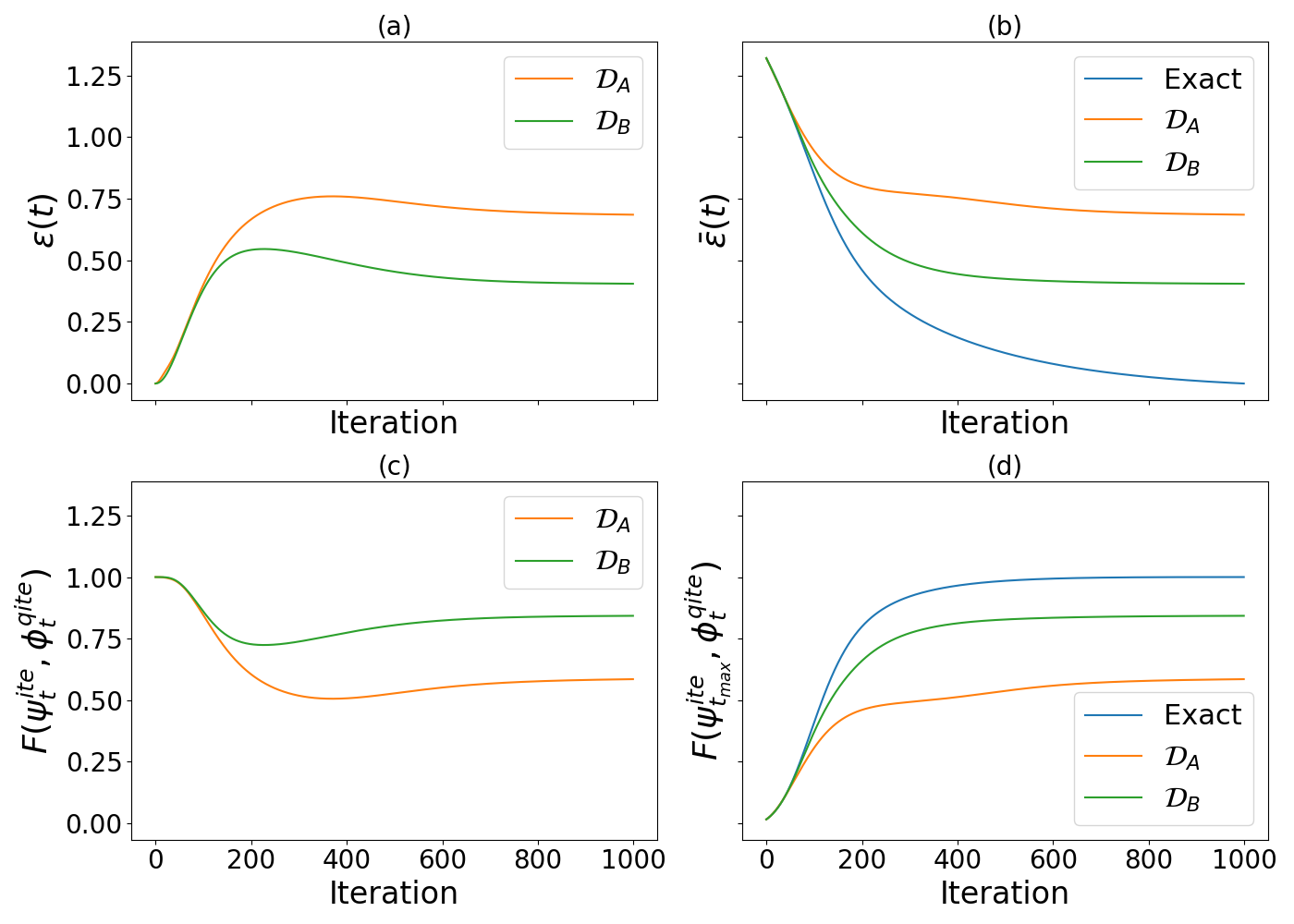
Figure 6: Error and fidelity results for the 8-qubit graph instance of Fig. 1b for different domains. (a) and (c) depict plots of $\varepsilon(t)$ (Eq. (17)) and $F(\psi^{ite}_{t},\phi^{qite}_{t})=|\langle\psi^{ite}_{t}|\phi^{qite}_{t}\rangle|^{2}$, respectively. (b) and (d) depict plots of $\bar{\varepsilon}(t)$ (Eq. (18)) and fidelity $F(\psi^{ite}_{t_{max}},\phi^{qite}_{t})=|\langle\psi^{ite}_{t_{max}}|\phi^{qite}_{t}\rangle|^{2}$. The blue line corresponds to calculate the fidelity with respect to the ITE state $|\psi^{ite}_{t}\rangle$.

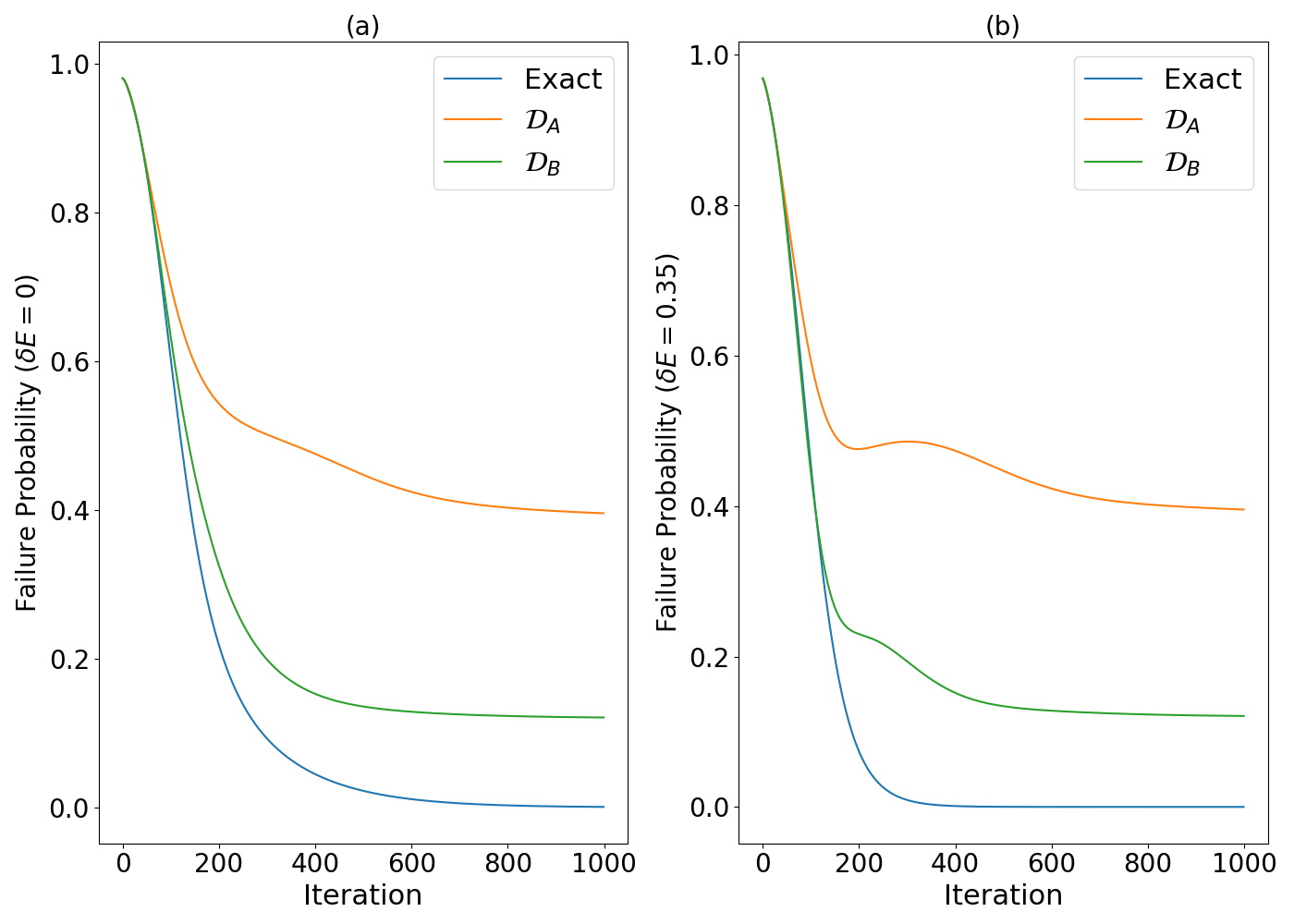
Figure 7: Failure probability for 8-qubit graph (Fig 1b). (a) $P_{F}^{ite}(t)$ (blue line) and $P_{F}^{qite}(t)$ for different domains and $\delta E=0$. (b) Similar to (a) but $\delta E=0.35$. This value represents the difference between the energy ground-state $E_{0}=-3$ and the energy of the first excited state $E_{1}=-2.65$. The degeneracy of the ground states is $g=4$ and for first excited states is $g=3$.

Figure 8: Failure probability $(P_{F}^{qite}(t))^{M}$ vs $M$ (number of shots) for 8-qubit graph for different iterations and domains.

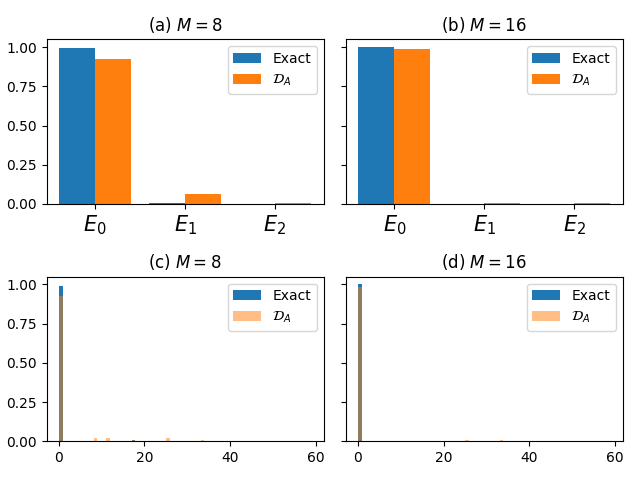
Figure 9: (a) and (b) show normalized histograms of obtained eigenvalues for 8-qubit graphs, with number of shots $M=8$ and $M=16$, respectively. (c) and (d) show normalized histograms of relative errors for $M=8$ and $M=16$ shots. The number of UD-MIS instances to make these plots was around 150.

B.2 Results for 10-qubits graphs

In this section we show the results for random graphs of 10 qubits. In this case we only consider 10 random graphs due to the numerical complexity of the calculations. As in the other cases, $\mathcal{D}_{A}$ performs well enough in terms of the failure probability, but $\mathcal{D}_{B}$ performs better than $\mathcal{D}_{A}$ in matching the ITE state for large number of iterations. Moreover, it is observed that the failure probability decreases when increasing the number of iterations, the number of shots, and the tolerable error. The number of iterations and shots do not need to be increased exponentially with the number of qubits.

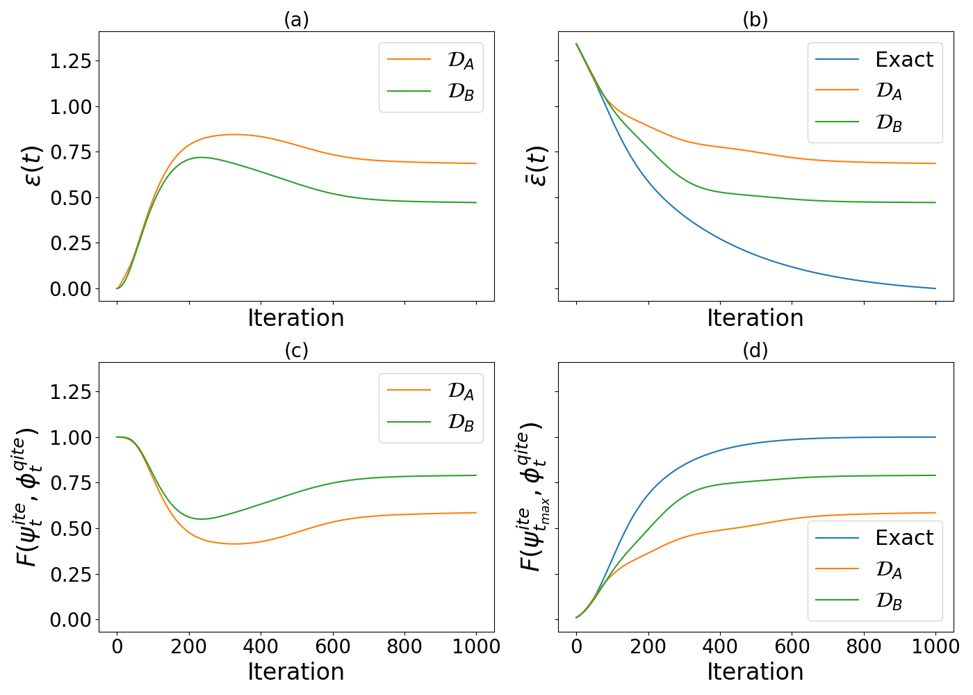
Figure 10: Error and fidelity results for the 10-qubit graph instance of Fig. 1c for different domains. (a) and (c) depict plots of $\varepsilon(t)$ (Eq. (17)) and $F(\psi^{ite}_{t},\phi^{qite}_{t})=|\langle\psi^{ite}_{t}|\phi^{qite}_{t}\rangle|^{2}$ respectively. (b) and (d) depict plots of $\bar{\varepsilon}(t)$ (Eq. (18)) and fidelity $F(\psi^{ite}_{t_{max}},\phi^{qite}_{t})=|\langle\psi^{ite}_{t_{max}}|\phi^{qite}_{t}\rangle|^{2}$. The blue line corresponds to calculate the fidelity with respect to the ITE state $|\psi^{ite}_{t}\rangle$.

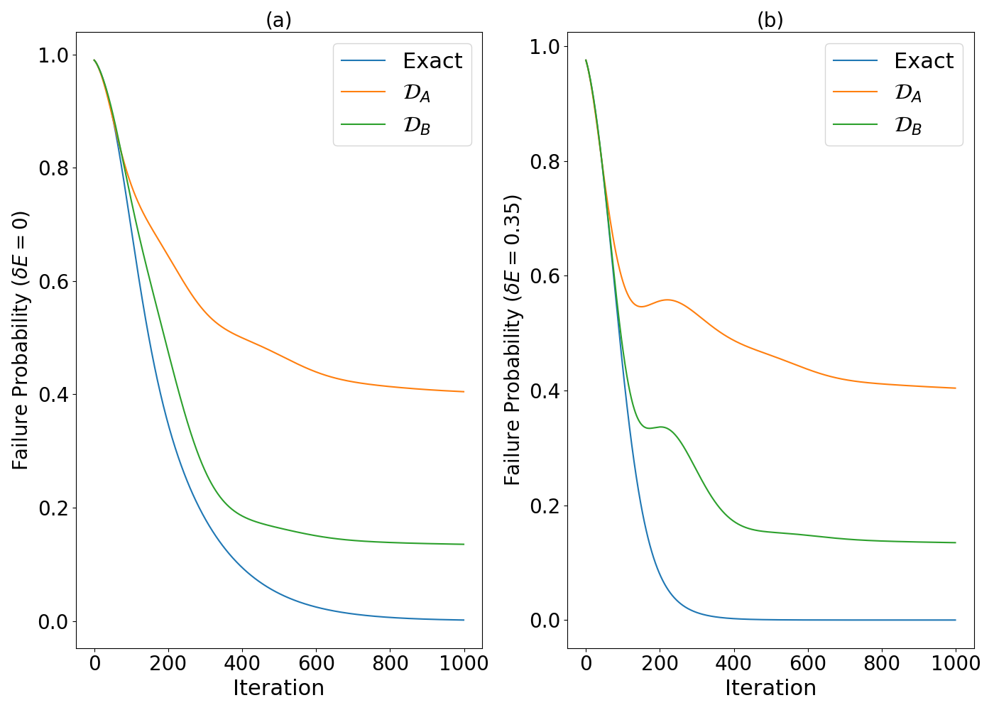
Figure 11: Failure probability for 10-qubit graph (Fig 1c). (a) $P_{F}^{ite}(t)$ (blue line) and $P_{F}^{qite}(t)$ for different domains and $\delta E=0$. (b) Similar to (a) but $\delta E=0.35$. This value represents the difference between the energy ground-state $E_{0}=-3$ and the energy of the first excited state $E_{1}=-2.65$. The degeneracy of the ground states is $g=9$ and for first excited states is $g=15$.

Figure 12: Failure probability $(P_{F}^{qite}(t))^{M}$ vs $M$ (number of shots) for 10-qubit graph for different number of iterations and domains.

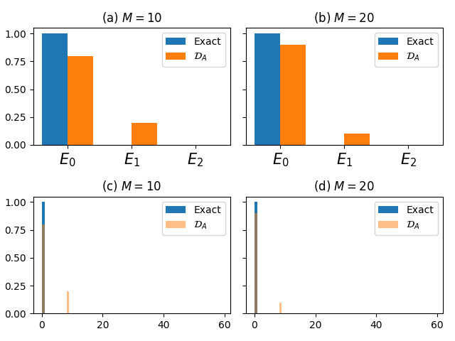
Figure 13: (a) and (b) show normalized histograms of obtained eigenvalues for 6-qubit graphs, with number of shots $M=10$ and $M=20$, respectively. (c) and (d) show normalized histograms of relative errors for $M=10$ and $M=20$ shots. The number of UD-MIS instances to make these plots was 10.

References

- [1] E. Farhi, J. Goldstone, S. Gutmann, J. Lapan, A. Lundgren, and D. Preda, “A quantum adiabatic evolution algorithm applied to random instances of an np-complete problem,” Science, vol. 292, p. 472–475, Apr. 2001.
- [2] A. Das and B. K. Chakrabarti, “Colloquium: Quantum annealing and analog quantum computation,” Reviews of Modern Physics, vol. 80, p. 1061–1081, Sept. 2008.
- [3] E. Farhi, J. Goldstone, and S. Gutmann, “A quantum approximate optimization algorithm,” 2014.
- [4] A. Peruzzo, J. McClean, P. Shadbolt, M.-H. Yung, X.-Q. Zhou, P. J. Love, A. Aspuru-Guzik, and J. L. O’Brien, “A variational eigenvalue solver on a photonic quantum processor,” Nature Communications, vol. 5, July 2014.
- [5] M. Cerezo, A. Arrasmith, R. Babbush, S. C. Benjamin, S. Endo, K. Fujii, J. R. McClean, K. Mitarai, X. Yuan, L. Cincio, and P. J. Coles, “Variational quantum algorithms,” Nature Reviews Physics, vol. 3, p. 625–644, Aug. 2021.
- [6] J. Tilly, H. Chen, S. Cao, D. Picozzi, K. Setia, Y. Li, E. Grant, L. Wossnig, I. Rungger, G. H. Booth, and J. Tennyson, “The variational quantum eigensolver: A review of methods and best practices,” Physics Reports, vol. 986, p. 1–128, Nov. 2022.
- [7] J. R. McClean, S. Boixo, V. N. Smelyanskiy, R. Babbush, and H. Neven, “Barren plateaus in quantum neural network training landscapes,” Nature Communications, vol. 9, Nov. 2018.
- [8] S. McArdle, T. Jones, S. Endo, Y. Li, S. C. Benjamin, and X. Yuan, “Variational ansatz-based quantum simulation of imaginary time evolution,” npj Quantum Information, vol. 5, Sept. 2019.
- [9] M. J. S. Beach, R. G. Melko, T. Grover, and T. H. Hsieh, “Making trotters sprint: A variational imaginary time ansatz for quantum many-body systems,” Physical Review B, vol. 100, Sept. 2019.
- [10] P. J. Love, “Cooling with imaginary time,” Nature Physics, vol. 16, p. 130–131, Feb. 2020.
- [11] M. Motta, C. Sun, A. T. K. Tan, M. J. O’Rourke, E. Ye, A. J. Minnich, F. G. S. L. Brandão, and G. K.-L. Chan, “Determining eigenstates and thermal states on a quantum computer using quantum imaginary time evolution,” Nature Physics, vol. 16, p. 205–210, Nov. 2019.
- [12] H. Nishi, T. Kosugi, and Y.-i. Matsushita, “Implementation of quantum imaginary-time evolution method on nisq devices by introducing nonlocal approximation,” npj Quantum Information, vol. 7, June 2021.
- [13] J.-L. Ville, A. Morvan, A. Hashim, R. K. Naik, M. Lu, B. Mitchell, J.-M. Kreikebaum, K. P. O’Brien, J. J. Wallman, I. Hincks, J. Emerson, E. Smith, E. Younis, C. Iancu, D. I. Santiago, and I. Siddiqi, “Leveraging randomized compiling for the quantum imaginary-time-evolution algorithm,” Physical Review Research, vol. 4, Aug. 2022.
- [14] C. Cao, Z. An, S.-Y. Hou, D. L. Zhou, and B. Zeng, “Quantum imaginary time evolution steered by reinforcement learning,” Communications Physics, vol. 5, Mar. 2022.
- [15] S.-H. Lin, R. Dilip, A. G. Green, A. Smith, and F. Pollmann, “Real- and imaginary-time evolution with compressed quantum circuits,” PRX Quantum, vol. 2, p. 010342, Mar 2021.
- [16] S. Barison, D. E. Galli, and M. Motta, “Quantum simulations of molecular systems with intrinsic atomic orbitals,” Physical Review A, vol. 106, Aug. 2022.
- [17] K. Yeter-Aydeniz, R. C. Pooser, and G. Siopsis, “Practical quantum computation of chemical and nuclear energy levels using quantum imaginary time evolution and lanczos algorithms,” npj Quantum Inf, vol. 6, p. 63, July 2020.
- [18] H. Kamakari, S.-N. Sun, M. Motta, and A. J. Minnich, “Digital quantum simulation of open quantum systems using quantum imaginary–time evolution,” PRX Quantum, vol. 3, Feb. 2022.
- [19] R. Alam, G. Siopsis, R. Herrman, J. Ostrowski, P. Lotshaw, and T. Humble, “Solving maxcut with quantum imaginary time evolution,” Quantum Inf Process, vol. 22, p. 281, Jul 2023.
- [20] N. M. Bauer, R. Alam, G. Siopsis, and J. Ostrowski, “Combinatorial optimization with quantum imaginary time evolution,” Phys. Rev. A, vol. 109, p. 052430, May 2024.
- [21] L. Zhou, S.-T. Wang, S. Choi, H. Pichler, and M. D. Lukin, “Quantum approximate optimization algorithm: Performance, mechanism, and implementation on near-term devices,” Physical Review X, vol. 10, June 2020.
- [22] J. Ostrowski, R. Herrman, T. S. Humble, and G. Siopsis, “Lower bounds on circuit depth of the quantum approximate optimization algorithm,” 2020.
- [23] R. Shaydulin, S. Hadfield, T. Hogg, and I. Safro, “Classical symmetries and the quantum approximate optimization algorithm,” Quantum Information Processing, vol. 20, Oct. 2021.
- [24] M. Medvidović and G. Carleo, “Classical variational simulation of the quantum approximate optimization algorithm,” npj Quantum Information, vol. 7, June 2021.
- [25] L. Zhu, H. L. Tang, G. S. Barron, F. A. Calderon-Vargas, N. J. Mayhall, E. Barnes, and S. E. Economou, “Adaptive quantum approximate optimization algorithm for solving combinatorial problems on a quantum computer,” Phys. Rev. Res., vol. 4, p. 033029, Jul 2022.
- [26] R. Herrman, P. C. Lotshaw, J. Ostrowski, T. S. Humble, and G. Siopsis, “Multi-angle quantum approximate optimization algorithm,” Scientific Reports, vol. 12, p. 6781, Apr 2022.
- [27] G. G. Guerreschi and A. Y. Matsuura, “Qaoa for max-cut requires hundreds of qubits for quantum speed-up,” Scientific Reports, vol. 9, May 2019.
- [28] J. S. Otterbach, R. Manenti, N. Alidoust, A. Bestwick, M. Block, B. Bloom, S. Caldwell, N. Didier, E. S. Fried, S. Hong, P. Karalekas, C. B. Osborn, A. Papageorge, E. C. Peterson, G. Prawiroatmodjo, N. Rubin, C. A. Ryan, D. Scarabelli, M. Scheer, E. A. Sete, P. Sivarajah, R. S. Smith, A. Staley, N. Tezak, W. J. Zeng, A. Hudson, B. R. Johnson, M. Reagor, M. P. da Silva, and C. Rigetti, “Unsupervised machine learning on a hybrid quantum computer,” 2017.
- [29] H. Pichler, S.-T. Wang, L. Zhou, S. Choi, and M. D. Lukin, “Quantum optimization for maximum independent set using rydberg atom arrays,” 2018.
- [30] L. Henriet, “Robustness to spontaneous emission of a variational quantum algorithm,” Physical Review A, vol. 101, Jan. 2020.
- [31] S. Ebadi, A. Keesling, M. Cain, T. T. Wang, H. Levine, D. Bluvstein, G. Semeghini, A. Omran, J.-G. Liu, R. Samajdar, X.-Z. Luo, B. Nash, X. Gao, B. Barak, E. Farhi, S. Sachdev, N. Gemelke, L. Zhou, S. Choi, H. Pichler, S.-T. Wang, M. Greiner, V. Vuletić, and M. D. Lukin, “Quantum optimization of maximum independent set using rydberg atom arrays,” Science, vol. 376, p. 1209–1215, June 2022.
- [32] R. S. Andrist, M. J. A. Schuetz, P. Minssen, R. Yalovetzky, S. Chakrabarti, D. Herman, N. Kumar, G. Salton, R. Shaydulin, Y. Sun, M. Pistoia, and H. G. Katzgraber, “Hardness of the maximum-independent-set problem on unit-disk graphs and prospects for quantum speedups,” Phys. Rev. Res., vol. 5, p. 043277, Dec 2023.
- [33] D. Lykov, J. Wurtz, C. Poole, M. Saffman, T. Noel, and Y. Alexeev, “Sampling frequency thresholds for the quantum advantage of the quantum approximate optimization algorithm,” npj Quantum Information, vol. 9, July 2023.
- [34] H. Yeo, H. E. Kim, and K. Jeong, “Approximating maximum independent set on rydberg atom arrays using local detunings,” 2024.
- [35] C. Dalyac, L.-P. Henry, M. Kim, J. Ahn, and L. Henriet, “Exploring the impact of graph locality for the resolution of the maximum- independent-set problem with neutral atom devices,” Phys. Rev. A, vol. 108, p. 052423, Nov 2023.
- [36] L. Henriet, L. Beguin, A. Signoles, T. Lahaye, A. Browaeys, G.-O. Reymond, and C. Jurczak, “Quantum computing with neutral atoms,” Quantum, vol. 4, p. 327, Sept. 2020.
- [37] M. Kim, J. Ahn, Y. Song, J. Moon, and H. Jeong, “Quantum computing with rydberg atom graphs,” Journal of the Korean Physical Society, vol. 82, pp. 827–840, May 2023.
- [38] H. Labuhn, D. Barredo, S. Ravets, S. de Léséleuc, T. Macrì, T. Lahaye, and A. Browaeys, “Tunable two-dimensional arrays of single rydberg atoms for realizing quantum ising models,” Nature, vol. 534, p. 667–670, June 2016.
- [39] D. Barredo, V. Lienhard, S. de Léséleuc, T. Lahaye, and A. Browaeys, “Synthetic three-dimensional atomic structures assembled atom by atom,” Nature, vol. 561, p. 79–82, Sept. 2018.
- [40] M. F. Serret, B. Marchand, and T. Ayral, “Solving optimization problems with rydberg analog quantum computers: Realistic requirements for quantum advantage using noisy simulation and classical benchmarks,” Physical Review A, vol. 102, Nov. 2020.
- [41] J. Hromkovič, Algorithmics for Hard Problems: Introduction to Combinatorial Optimization, Randomization, Approximation, and Heuristics. Springer Berlin, Heidelberg, 2004.
- [42] T. Matsui, “Approximation algorithms for maximum independent set problems and fractional coloring problems on unit disk graphs,” in Discrete and Computational Geometry (J. Akiyama, M. Kano, and M. Urabe, eds.), (Berlin, Heidelberg), pp. 194–200, Springer Berlin Heidelberg, 2000.
- [43] G. K. Das, G. D. da Fonseca, and R. K. Jallu, “Efficient independent set approximation in unit disk graphs,” Discrete Applied Mathematics, vol. 280, pp. 63–70, 2020. Algorithms and Discrete Applied Mathematics (CALDAM 2016).
- [44] E. J. van Leeuwen, “Approximation algorithms for unit disk graphs,” in Graph-Theoretic Concepts in Computer Science (D. Kratsch, ed.), (Berlin, Heidelberg), pp. 351–361, Springer Berlin Heidelberg, 2005.
- [45] G. D. da Fonseca, V. G. a. Pereira de Sá, and C. M. H. de Figueiredo, “Shifting coresets: Obtaining linear-time approximations for unit disk graphs and other geometric intersection graphs,” International Journal of Computational Geometry & Applications, vol. 27, no. 04, pp. 255–276, 2017.
- [46] T. Nieberg, J. Hurink, and W. Kern, “A robust ptas for maximum weight independent sets in unit disk graphs,” in Graph-Theoretic Concepts in Computer Science (J. Hromkovič, M. Nagl, and B. Westfechtel, eds.), (Berlin, Heidelberg), pp. 214–221, Springer Berlin Heidelberg, 2005.