A systematical study of the nucleon form factors with the pion cloud effect

Abstract

The electromagnetic and gravitational form factors of the nucleon are studied simultaneously using a covariant quark-diquark approach, and the pion cloud effect on the form factors is explicitly discussed. In this study, the electromagnetic form factors are first calculated to determine the parameters of our approach. Then, the gravitational form factors of the nucleon are evaluated with the same parameters and the cloud effect is addressed. The mechanical properties, including mass radii, energy densities, and spin distributions, are shown and discussed.

1 Introduction

Understanding the particle structure remains a fundamental topic in hadron physics. Form factors carry a wealth of information, serving as a useful tool for exploring the internal structure of particles. It is well known that for a spin-1/2 hadron, its electromagnetic form factors (EMFFs) are related to the electromagnetic properties including the distributions of the electric charge, the magnetic moment and the charge radius. Similarly, the gravitational form factors (GFFs), which are derived from the matrix element of the symmetric energy-momentum tensor (EMT) [1], could provide information about the interior of the particle such as the mass and spin distributions.

A significant number of experiments have detected the EMFFs of the nucleon [2]. However, due to the impracticality of directly detecting the graviton coupling with the matter field, the GFFs cannot be experimentally assessed. Fortunately, deeply virtual Compton scattering (DVCS)[3], a process in which quarks within the particle absorb a virtual photon and subsequently emit a high-energy real photon, offers an another chance for accessing the GFFs. With the help of DVCS, one can obtain the generalized parton distributions [4] and extract GFFs via the sum rule [5, 6]. In 2018, the GFF $D_{0}(t)$ of the proton was first extracted [7].

Despite the difficulty of detecting GFFs experimentally, GFFs can be studied theoretically based on the similar process with EMFFs. The GFFs of the nucleon have been studied with different approaches including the lattice QCD [8, 9], the chiral quark-soliton model [10, 11], the Skyrme model [12], the light-front quark-diquark model [13], the large $N_{c}$ quark model [14], the light-cone QCD sum rule [15, 16], and so on [17]. Besides, the studies of GFFs of other particles including pion [18, 19, 20], $K$ meson [20], $\rho$ meson [21, 22, 20], and the spin-3/2 baryons [23, 24, 25, 26] have also been carried out.

In this paper, the form factors of the nucleon are calculated with a covariant quark-diquark approach. The nucleon, a three-body system, is treated as the combination of a quark and a diquark, which could effectively simplify the numerical calculations. The quark-diquark approach has been applied to our previous study on the decuplet barons [25, 24], and will be apply to our future study on the $N-\Delta$ transition.

Furthermore, the pion cloud of the nucleon is incorporated into this study. In some works focusing on the EMFFs [27, 28], it has been demonstrated that the pion cloud results in a notable enhancement in the magnitude of the magnetic moments and influences the shape of the electric form factor of the neutron obviously. However, the pion cloud effect on the gravitational form factors has seldom been discussed. In this paper, the GFFs and the EMFFs of the nucleon are calculated with the same parameters simultaneously to evaluate the influence of the pion cloud.

This paper is organized as follows. Section II gives the definitions of the EMFFs and the GFFs of the nucleon. Moreover, the covariant quark-diquark approach and the pion cloud effect are introduced here. In Section III, the numerical results are given, and the electromagnetic and mechanical properties of the nucleon are derived further from the electromagnetic and gravitational form factors. Furthermore, the pion cloud effect on the EMFFs and the GFFs is discussed in detail. Finally, a brief discuss and a summary are displayed in Section IV.

2 Form Factors And Quark-diquark Approach

2.1 Electromagnetic and gravitational form factors

For the nucleon, a spin-1/2 particle, the matrix element of electromagnetic current $J^{\mu}$ are expressed as [29]

$$\begin{split}\langle p^{\prime},\lambda^{\prime}|\hat{J}^{\mu}|p,\lambda\rangle&=\overline{u}\left(p^{\prime},\lambda\right)\biggl{[}\gamma^{\mu}F_{1}\left(t\right)+\frac{i\sigma^{\mu q}}{2M_{N}}F_{2}\left(t\right)\biggr{]}u\left(p,\lambda\right),\end{split}$$ (1)

where $\sigma^{\nu q}=\sigma^{\nu\rho}q_{\rho}$, $M_{N}$ stands for the mass of the nucleon, and $u\left(p,\lambda\right)$ is the Dirac spinor with normalization as $\overline{u}\left(p,\lambda\right)u\left(p,\lambda\right)=2M_{N}$. The kinematical variables in Eq. (1) are defined as follow, $P^{\mu}=\left(p^{\mu}+p^{\prime\mu}\right)/2$, $q^{\mu}=p^{\prime\mu}-p^{\mu}$ and $t=q^{2}$, where $p$ ($p^{\prime}$) is the initial (final) momentum.

The electric and magnetic form factors are defined as [30]

$$G_{E}(t)=F_{1}(t)+\frac{t}{4M_{N}^{2}}F_{2}(t),$$ (2a)

$$G_{M}(t)=F_{1}(t)+F_{2}(t).$$ (2b)

When the squared momentum transfer $t$ goes to zero, there are relations $Q_{e}=G_{E}(0)$ and $\mu=\frac{e}{2M_{N}}G_{M}(0)$, where $Q_{e}$ and $\mu$ respectively stand for the charge quantum number and the magnetic moment carried by the particle.

The charge and magnetic radii of the particle can be derived from their form factors

$${\langle r^{2}_{E}\rangle}=\left.\frac{6}{G_{E}(0)}\frac{d}{dt}G_{E}(t)\right|_{t=0},\quad{\langle r^{2}_{M}\rangle}=\left.\frac{6}{G_{M}(0)}\frac{d}{dt}G_{M}(t)\right|_{t=0}.$$ (3)

Specially, for the neutral particle, the charge radius is defined as

$${\langle r^{2}_{E}\rangle}=\left.6\frac{d}{dt}G_{E}(t)\right|_{t=0}.$$ (4)

Similarly, the GFFs of the nucleon are obtained from the matrix element of the EMT current, which is defined as [29]

$$\begin{split}\langle p^{\prime},\lambda^{\prime}|\hat{T}^{\mu\nu}|p,\lambda\rangle&=\overline{u}\left(p^{\prime},\lambda^{\prime}\right)\biggl{[}\frac{P^{\mu}P^{\nu}}{M_{N}}F_{1,0}(t)+\frac{\left(q^{\mu}q^{\nu}-g^{\mu\nu}q^{2}\right)}{M_{N}}F_{2,0}(t)+M_{N}g^{\mu\nu}F_{3,0}(t)\\ &+\frac{i}{4M_{N}}P^{\{\mu}\sigma^{\nu\}q}F_{4,0}(t)\biggl{]}u(p,\lambda),\end{split}$$ (5)

where $P^{\{\mu}\sigma^{\nu\}q}=P^{\mu}\sigma^{\nu q}+P^{\nu}\sigma^{\mu q}$. Notice that $F_{3,0}(t)$ is a non-conserving term which vanishes when considering the total EMT of the quark and the gluon. Thus, we simply ignore it here.

The gravitational multipole form factors (GMFFs) $\varepsilon_{0}(t)$, $\mathcal{J}_{1}(t)$ and $D_{0}(t)$ are derived from the matrix element of the EMT current in the Breit frame, where $P\cdot q=0$ and $q^{2}=4(M^{2}-E^{2})$ with the initial and final momenta defined as $p=(E,\bm{q}/2)$ and $p^{\prime}=(E,-\bm{q}/2)$. The relations among the GMFFs and the GFFs are [10]

$$\varepsilon_{0}(t)=F_{1,0}(t)+ \frac{t}{4M_{N}^{2}}\left[-F_{1,0}(t)-4F_{2,0}(t)+F_{4,0}(t)\right],$$ (6a)

$$\mathcal{J}_{1}(t)=\frac{1}{2}F_{4,0}(t),$$ (6b)

$$D_{0}(t)=4F_{2,0}(t).$$ (6c)

$\varepsilon_{0}(t)$ and $\mathcal{J}_{1}(t)$ are related to the mass and the spin of the particle, respectively. The mass radius of the particle can be derived from $\varepsilon_{0}(t)$

$$\langle r^{2}_{m}\rangle=\left.\frac{6}{\varepsilon_{0}(0)}\frac{d}{dt}\varepsilon_{0}(t)\right|_{t=0}.$$ (7)

By applying Fourier transformation to $\varepsilon_{0}(t)$ and $\mathcal{J}_{1}(t)$, one can get the energy and angular momentum densities of the particle as

$$\mathcal{E}_{0}(r)=M_{N}\int\frac{d^{3}q}{(2\pi)^{3}}e^{-i\bm{q}\cdot\bm{r}}\varepsilon_{0}(t),$$ (8)

$$\rho_{J}(r)=-\frac{1}{3}r\frac{d}{dr}\int\frac{d^{3}q}{(2\pi)^{3}}e^{-i\bm{q}\cdot\bm{r}}\mathcal{J}_{1}(t).$$ (9)

$D_{0}(t)$, correlated with the so-called D-term $D=D_{0}(0)$, is believed to be connected with the pressure and shear force distributions within the particle in the classical physics, which can be expressed as[1]

$$p(r)=\frac{1}{6M_{N}}\frac{1}{r^{2}}\frac{d}{dr}r^{2}\frac{d}{dr}\widetilde{D}_{0}(r),$$ (10)

$$s(r)=-\frac{1}{4M_{N}}r\frac{d}{dr}\frac{1}{r}\frac{d}{dr}\widetilde{D}_{0}(r),$$ (11)

where $\widetilde{D}_{0}(r)=\int\frac{d^{3}q}{(2\pi)^{3}}e^{-i\bm{q}\cdot\bm{r}}D_{0}(t)$.

2.2 Quark-diquark approach

To simplify the calculation, the nucleon is treated as the combination of a quark and either a scalar (spin-0) diquark or an axialvector (spin-1) diquark. The flavor wave functions of the proton and the neutron are written as [31]

$$|p\rangle=\cos{\theta}|u(ud)_{s}\rangle+\sin{\theta}\left[\sqrt{\frac{2}{3}}|d(uu)_{a}\rangle-\sqrt{\frac{1}{3}}|u(ud)_{a}\rangle\right],$$ (12a)

$$|n\rangle=\cos{\theta}|d(ud)_{s}\rangle+\sin{\theta}\left[-\sqrt{\frac{2}{3}}|u(dd)_{a}\rangle+\sqrt{\frac{1}{3}}|d(ud)_{a}\rangle\right],$$ (12b)

where $(q_{1}q_{2})_{s}$ and $(q_{1}q_{2})_{a}$ respectively represent the scalar and the axialvector diquarks consisting of quarks $q_{1}$ and $q_{2}$, and $\theta$ is the mixing angle between the scalar and the axialvector diquarks.

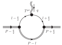
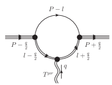
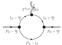
Figure 1: Feynman diagrams for the coupling processes of the EMT with the quark (a) and the diquark (b). When the EMT current couples with the diquark, the internal structure of the diquark (c) is considered.

The GFFs of the nucleon are derived from the matrix element of the EMT, and for the EMFFs, the EMT current $T^{\mu\nu}$ is replaced by the electromagnetic current $J^{\mu}$. The detailed calculation process is presented in our previous work on $\Delta$ [24], and here we give a brief introduction to the calculation of the GFFs.

According to the wave functions of the nucleon in Eq.(12), the matrix element can be written as the sum of that contributed by the quark and the diquark

$$\langle p^{\prime},\lambda^{\prime}|\hat{T}^{\mu\nu}|p,\lambda\rangle=\langle p^{\prime},\lambda^{\prime}|\hat{T}^{\mu\nu}_{q}|p,\lambda\rangle+\langle p^{\prime},\lambda^{\prime}|\hat{T}^{\mu\nu}_{D}|p,\lambda\rangle.$$ (13)

Figures 1 and 1 give the Feynman diagrams of the coupling processes with the quark and the diquark respectively.

Since the diquark in Fig. 1 can be regarded as a scalar or axialvector one, the form factors should be discussed separately. Assuming that the nucleon is a composite of a quark and a scalar diquark, the matrix element contributed by the quark can be written as

$$\begin{split}\langle p^{\prime},\lambda^{\prime}|\hat{T}^{\mu\nu}_{q}|p,\lambda\rangle&=\overline{u}(p^{\prime},\lambda^{\prime})\int\frac{d^{4}l}{(2\pi)^{4}}\frac{c^{2}}{\mathcal{D}}\Gamma_{s}(\not{l}+\frac{\not{q}}{2}+m_{q})\Lambda^{\mu\nu}(t)(\not{l}-\frac{\not{q}}{2}+m_{q})\Gamma_{s}u(p,\lambda),\end{split}$$ (14)

where $\Lambda^{\mu\nu}(t)$ stands for the interaction vertex between the EMT current and the quark.

Firstly, considering a point-like quark without the pion cloud, the Lagrangian is written as

$$\mathcal{L}=\frac{i}{2}\overline{\psi}_{q}\gamma^{\mu}{\mathop{\partial}\limits^{\leftrightarrow}}_{\mu}\psi_{q}+m_{q}\overline{\psi}_{q}\psi_{q},$$ (15)

where ${\mathop{\partial}\limits^{\leftrightarrow}}_{\mu}={\mathop{\partial}\limits^{\rightarrow}}_{\mu}-{\mathop{\partial}\limits^{\leftarrow}}_{\mu}$. The EMT of the quark are derived from the Lagrangian as

$$T^{\mu\nu}=\frac{i}{4}\overline{\psi}_{q}\gamma^{\mu}{\mathop{\partial^{\nu}}\limits^{\leftrightarrow}}\psi_{q}+\frac{i}{4}\overline{\psi}_{q}\gamma^{\nu}{\mathop{\partial^{\mu}}\limits^{\leftrightarrow}}\psi_{q}.$$ (16)

Therefore, the vertex reads

$$\Lambda^{\mu\nu}_{PL}=l^{\mu}\gamma^{\nu}+l^{\nu}\gamma^{\mu}.$$ (17)

However, the vertex is modified due to the pion cloud effect, which will be discussed later.

$\Gamma_{s}$ stands for the quark-diquark-nucleon vertex borrowed from Ref. [32]. For the scalar diquark and the axialvector diquark, the vertexes are different, which read

$$\Gamma_{s}=c_{s},\quad\Gamma_{a}^{\mu}=c_{a}\gamma^{\mu}\gamma^{5}$$ (18)

respectively. Furthermore, an extra scalar function $\Xi(p_{1},p_{2})$ is attached to the vertex to simulate the bound state of the nucleon. Generally, the scalar function should be obtained through solving the Bethe-Salpeter equation. Here, we take an ansatz to simplify the calculation [33], which reads

$$\Xi(p_{1},p_{2})=\frac{c}{(p_{1}^{2}-m_{R}^{2}+i\epsilon)(p_{2}^{2}-m_{R}^{2}+i\epsilon)},$$ (19)

where $p_{1}$ and $p_{2}$ stand for the momenta of the quark and the diquark and $m_{R}$ in (19) is a cutoff parameter which will be discussed later. $\mathcal{D}$ stands for all the denominators from the propagators and the scalar functions as

$$\begin{split}\mathcal{D}=&\left[\left(l+\frac{q}{2}\right)^{2}-m_{q}^{2}+i\epsilon\right]\left[\left(l-\frac{q}{2}\right)^{2}-m_{q}^{2}+i\epsilon\right]\left[\left(l-P\right)^{2}-m_{D}^{2}+i\epsilon\right]\\ &\times\left[\left(l+\frac{q}{2}\right)^{2}-m_{R}^{2}+i\epsilon\right]\left[\left(l-\frac{q}{2}\right)^{2}-m_{R}^{2}+i\epsilon\right]\left[\left(l-P\right)^{2}-m_{R}^{2}+i\epsilon\right]^{2}.\end{split}$$ (20)

The matrix element contributed by the diquark can also be evaluated in the similar way. For the scalar diquark, the matrix element reads

$$\begin{split}\langle p^{\prime},\lambda^{\prime}|\hat{T}^{\mu\nu}_{D}|p,\lambda\rangle&=\overline{u}(p^{\prime},\lambda^{\prime})\int\frac{d^{4}l}{(2\pi)^{4}}\frac{c^{2}}{\mathcal{D}^{\prime}}\Gamma_{s}(\not{P}-\not{l}+m_{q})X^{\mu\nu}\Gamma_{s}u(p,\lambda).\end{split}$$ (21)

The structure of $\mathcal{D}^{\prime}$ is similar with Eq. (20) but the masses are changed. $X^{\mu\nu}$ is an effective EMT current of the spin-0 diquark, which is derived from the inner structure of the diquark as

$$X^{\mu\nu}=\sum_{q}\langle p_{D}^{\prime},\lambda_{D}^{\prime}|\hat{T}^{\mu\nu}_{q}|p_{D},\lambda_{D}\rangle,$$ (22)

where $\langle p_{D}^{\prime},\lambda^{\prime}_{D}|\hat{T}^{\mu\nu}_{q}|p_{D},\lambda_{D}\rangle$ stands for the matrix element originated from Fig. 1. The effective current can be expressed as [29]

$$X^{\mu\nu}=2P^{\mu}_{D}P^{\nu}_{D}F_{1,0}^{D}(t)+2\left(q^{\mu}q^{\nu}-g^{\mu\nu}q^{2}\right)F_{2,0}^{D}(t)+2m_{D}^{2}g^{\mu\nu}F_{3,0}^{D}(t),$$ (23)

where $P_{D}=(p^{\prime}_{D}+p_{D})/2=l$, $q=q_{D}=p^{\prime}_{D}-p_{D}$, and $F_{1,0}^{D}(t),F_{2,0}^{D}(t)$ and $F_{3,0}^{D}(t)$ are the form factors of the scalar diquark obtained with the similar procedure in (14)-(19). The quark-quark-diquark vertex is borrowed from Ref. [34], which reads $\gamma^{5}$ for the scalar diquark and $\gamma^{\mu}$ for the axialvector diquark.

For the axialvector diquark, the effective current $X^{\mu\nu,\beta^{\prime}\beta}$ is derived from Fig. 1 similarly, which can be expressed as [29]

$$\begin{split}-\epsilon^{*}_{\beta^{\prime}}(p^{\prime}_{D},\lambda^{\prime}_{D})X^{\mu\nu,\beta^{\prime}\beta}\epsilon_{\beta}(p_{D},\lambda_{D})=&\sum_{q}\langle p_{D}^{\prime},\lambda^{\prime}_{D}|\hat{T}^{\mu\nu}_{q}|p_{D},\lambda_{D}\rangle\\ =&-\epsilon^{*}_{\beta^{\prime}}(p^{\prime}_{D},\lambda^{\prime}_{D})\biggl{[}2P^{\mu}_{D}P^{\nu}_{D}\left(g^{\beta\beta^{\prime}}F_{1,0}^{D}(t)-\frac{q^{\beta}q^{\beta^{\prime}}}{2m_{D}^{2}}F_{1,1}^{D}(t)\right)\\ &+2\left(q^{\mu}q^{\nu}-g^{\mu\nu}q^{2}\right)\left(g^{\beta\beta^{\prime}}F_{2,0}^{D}(t)-\frac{q^{\beta}q^{\beta^{\prime}}}{2m_{D}^{2}}F_{2,1}^{D}(t)\right)-P_{D}^{\{\mu}g^{\nu\}[\beta^{\prime}}q^{\beta]}F_{4,0}^{D}(t)\\ &-\left(q^{\{\mu}g^{\nu\}[\beta^{\prime}}q^{\beta]}-2q^{\beta}q^{\beta^{\prime}}g^{\mu\nu}-g^{\beta^{\prime}\{\mu}g^{\nu\}\beta}q^{2}\right)F_{5,0}^{D}(t)\biggl{]}\epsilon_{\beta}(p_{D},\lambda_{D}).\end{split}$$ (24)

The transition current between the scalar diquark and the axialvector diquark also contributes to the matrix element. As shown in Eq. (12), only diquark $(ud)$ participates in the transition process. As an analogy to the electromagnetic transition current [28], the effective current can be written as

$$\begin{split}\epsilon^{*}_{\beta^{\prime}}(p^{\prime}_{D},\lambda^{\prime}_{D})X^{\mu\nu,\beta^{\prime}}_{s\rightarrow a}&=\langle p_{D}^{\prime},\lambda^{\prime}_{D}|\hat{T}^{\mu\nu}_{u}|p_{D},\lambda_{D}\rangle-\langle p_{D}^{\prime},\lambda^{\prime}_{D}|\hat{T}^{\mu\nu}_{d}|p_{D},\lambda_{D}\rangle\\ &=i\epsilon^{*}_{\beta^{\prime}}(p^{\prime}_{D},\lambda^{\prime}_{D})P^{\{\mu}\varepsilon^{\nu\}\beta^{\prime}{P_{D}}q}F^{D}_{s\rightarrow a}(t),\end{split}$$ (25)

where $F^{D}_{s\rightarrow a}(t)$ is the form factor of the transition process from the scalar diquark to the axialvector diquark. For the reverse process, the effective current has the similar structure but $F^{D}_{s\rightarrow a}(t)=-F^{D}_{a\rightarrow s}(t)$.

2.3 Pion cloud effect

In this paper, it is assumed that the quark is no longer a point-like particle, but a so-called dressed quark coupling with the pion. Similar with the diquark, the inner structure of the quark is considered. Therefore, the interaction vertex between the quark and the EMT current is modified accordingly, which reads

$$\Lambda^{\mu\nu}\left(t\right)=l^{\{\mu}\gamma^{\nu\}}F_{1,0}^{q}(t)+2\left(q^{\mu}q^{\nu}-g^{\mu\nu}q^{2}\right)F_{2,0}^{q}(t)+\frac{i}{2}l^{\{\mu}\sigma^{\nu\}q}F_{4,0}^{q}(t),$$ (26)

where the form factors $F_{i,0}^{q}(t)$ are the mixture between the point-like quark and the dressed quark. Assuming that the quark discussed is on-shell, Eq. (26) can be transformed into the same structure as Eq.(5) with the on-shell identities in Ref. [35].

The form factors $F_{i,0}^{q}(t)$ can be expressed as

$$F_{i,0}^{q}=ZF_{i,0}^{PL}+\left(1-Z\right)(f_{i,0}^{q}+2f_{i,0}^{\pi}),\quad i=1,2,4,$$ (27)

where $F_{1,0}^{PL}=1$, $F_{k,0}^{PL}=0$ ($k=2,4$) are the form factors of the point-like quark, and $f_{i,0}^{q}$ and $f_{i,0}^{\pi}$ ($i=1,2,4$) are the form factors originated from the second and third figures in Fig. 2 respectively.

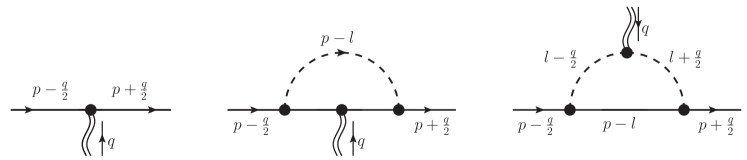
Figure 2: The coupling process between the EMT and the quark with the pion cloud correction. The first figure illustrates the coupling process without the pion cloud. In the second and third figures, the EMT current respectively couples with the quark and the pion cloud, and the body form factors $f_{i,0}^{q}$ and $f_{i,0}^{\pi}\,(i=1,2,4)$ are originated from the two figures.

The factor $Z$ stands for the possibility to strike a quark without the pion cloud [28], and it is derived from the self-energy $\Sigma(p)$ of the pion loop as

$$\begin{split}Z=1+\left.\frac{\partial\Sigma(p)}{\partial\not{p}}\right|_{\not{p}=m_{q}}.\end{split}$$ (28)

The self-energy is originated from Fig. 3, which reads

$$\Sigma(p)=\int\frac{d^{4}l}{(2\pi)^{4}}\gamma^{5}\tau_{i}S(p-l)\gamma^{5}\tau_{i}\tau_{\pi}(l),$$ (29)

where $\tau_{\pi}(p)=\frac{iZ_{\pi}}{p^{2}-m_{\pi}^{2}+i\varepsilon}$ is the $t$-matrix of pion with the pole approximation, which is introduced detailedly in Ref. [28].

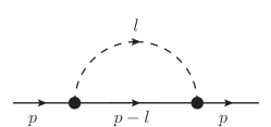
Figure 3: Pion loop correction of the quark self-energy. The solid line represents the quark and the dashed curve stands for the pion. The dark dot symbolises the quark-pion vertex $\gamma_{5}\tau_{i}$.

Similarly, for the electromagnetic current $J^{\mu}$, the structure of the effective vertex is the same as the matrix element of the vector operator, which reads $\Lambda^{\mu}\left(t\right)=\gamma^{\mu}F_{1}^{q}\left(t\right)+\frac{i\sigma^{\mu q}}{2M_{q}}F_{2}^{q}\left(t\right)$. The definitions of $F_{1}^{q}(t)$ and $F_{2}^{q}(t)$ can be refereed to Ref. [28] for detail.

3 Numerical Results

3.1 Parameter determination

The model parameters, including the baryon mass $M_{N}$, pion mass $m_{\pi}$, quark mass $m_{q}$, diquark mass $m_{D}$, the mixing angle $\theta$ and the cutoff parameter $m_{R}$ introduced in Eq. (19), need to be determined. Two sets of parameters are used in the calculation separately, which are listed in Tab. 1. The parameters in Set A are determined through fitting the experiment results, while the parameters in Set B are the same as those used in our previous study on $\Delta$ to facilitate our future study on the $N-\Delta$ transition[24]. Here we primarily focus on the determination of the parameters in Set A and show an analysis of the results obtained with Set A parameters.

	$M_{N}$/GeV	$m_{D}$/GeV	$m_{q}$/GeV	$m_{\pi}$/GeV	$m_{R}$/GeV	$Z_{\pi}$	$Z$	$\sin^{2}\theta$
Set A	0.938	0.6	0.39	0.14	1.4	17.39	0.77	0.23
Set B	1.085	0.76	0.4	0.14	1.6	18.16	0.77	0.18

Table 1: Parameters used in this work.

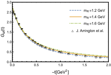
Figure 4: $G_{M}(t)$ of the proton with different $m_{R}$. The dashed, solid and the dotted-dashed curves respectively represent the results with $m_{R}=1.2$ GeV, 1.4 GeV, and 1.6 GeV. The triangles represent the data extracted from the experiment in Ref. [36].

To ensure that the quark and the diquark exist in the bound state, the input masses must satisfy the relations $M_{N}<m_{q}+m_{D}$ and $m_{D}<2m_{q}$. In set A, the masses of the nucleon and the pion are adapted from Ref. [37], and we assume that the scalar and the axialvector diquarks have the same masses. In set B, the nucleon mass is no longer $0.938$ GeV, but the average of the masses of the nucleon and the $\Delta$ resonance, which could offer convenience to our future study on the $N-\Delta$ transition. Thus, the masses of the quark and the diquark are larger than those in Set A to satisfy the bound state conditions. Figure 4 shows the $G_{M}(t)$ of the proton calculated with Set A parameters and the values of $m_{R}$ varies from 1.2 GeV to 1.6 GeV. All the results obtained are consistent with the experiment results in Ref. [36], and when $m_{R}$ goes up in a certain range, the magnetic moment $\mu$ and magnetic radius $r_{M}$ slightly decreases. Here we choose $m_{R}=1.4$ GeV, slightly smaller than that we used in our previous study about $\Delta$ [24], to keep $m_{R}$ positively correlated with the baryon mass. $Z$ and $Z_{\pi}$ are the normalization factors introduced in Eq. (28) and (29). $Z_{\pi}$ is originated from its self-energy, which can be referred to Ref. [28] for the detailed definition. Moreover, with the normalization condition of the proton EMFF $G_{E}(0)=1$, the normalization constants $C_{s}=cc_{s}$ and $C_{a}=cc_{a}$ introduced in Eq. (18) and Eq. (19) are determined respectively.

Tables 2 list the calculated electromagnetic properties with different $\theta$ respectively. As seen in Eq. (12), $\theta=0$ indicates that the nucleon is entirely made of a quark and a scalar diquark. Notice that when $\theta=0$ or $\theta=\pi/2$, the scalar-vector transition process will no longer contribute to the form factors. Therefore, when $\theta=0$ or $\theta=\pi/2$, especially for $\theta=0$, the obtained magnetic moments are smaller. According to Tab. 2, scalar diquark could provide larger electromagnetic radii, while the magnetic moments are smaller than those provided by the axialvector diquark. When only considering the scalar diquark, the magnetic moments of both the proton and the neutron are much smaller than the experiment results. In regard of the GFFs, the mixing angle has little influence on the energy and angular momentum form factors, while $D_{0}(t)$ is significantly increased as $\theta$ increases. $\theta$ is determined through fitting the experiment data of the EMFFs of the nucleon. [36, 38, 39, 37] Here, we choose $\sin^{2}\theta=0.23$, which means that the scalar diquark takes a dominant position. As for Set B, we choose $\sin^{2}\theta=0.18$ using the similar procedure.

$\theta$	$\mu_{p}/\mu_{N}$	$\sqrt{\langle r^{2}_{Ep}\rangle}/\text{fm}$	$\sqrt{\langle r^{2}_{Mp}\rangle}/\text{fm}$	$\mu_{n}/\mu_{N}$	$\langle r^{2}_{En}\rangle/\text{fm}^{2}$	$\sqrt{\langle r^{2}_{Mn}\rangle}/\text{fm}$
0	1.89	0.89	0.91	-1.12	-0.22	0.99
$\pi/6$	2.83	0.89	0.90	-1.93	-0.20	0.95
$\pi/4$	3.16	0.87	0.89	-2.14	-0.17	0.94
$\pi/2$	2.80	0.84	0.86	-1.52	-0.10	0.95
PDG [37]	2.79	0.84	0.851$\pm$0.026	-1.91	-0.12	$0.864^{+0.009}_{-0.008}$

Table 2: Electromagnetic properties of the nucleon with different mixing angle $\theta$, compared with those from PDG [37]. Note that $\mu_{N}=e/(2M_{N})$.

3.2 EMFFs of the nucleon

The calculated EMFFs of the nucleon are illustrated in Fig. 5. The Set A results are illustrated with black solid curves, showing a good agreement with the data extracted from the experiments [36, 38, 39]. The magnetic moments of the nucleon are

$$\mu_{p}=2.79\,\mu_{N}\quad\quad\mu_{n}=-1.90\,\mu_{N},$$ (30)

and the charge radii derived from $G_{E}(t)$ are

$$\sqrt{\langle r^{2}_{Ep}\rangle}=0.89\,\text{fm}\quad\quad\langle r^{2}_{En}\rangle=-0.20\,\text{fm}^{2}.$$ (31)

Furthermore, the detailed electromagnetic properties, including magnetic moments and electromagnetic radii are listed in Tab. 3. The results obtained without the pion cloud are illustrated as the red dashed curves in Fig. 5. It is evident that the pion cloud has little effect on the electric form factor of the proton. Conversely, it distinctly changes the shape of the neutron electric form factor, raising the magnitude of the charge radius and depressing the electric form factor in large $\left|t\right|$. With regard to the magnetic form factors, the pion cloud increases the magnetic moments of the proton and the neutron by about $15\%$ and $37\%$ respectively, while the effect is insignificant with large $\left|t\right|$. Furthermore, the pion cloud exerts an influence on the radii of the nucleon as listed in Tab. 3. Comparing with those obtained without the pion cloud correction, both the charge and magnetic radii of the nucleon increase, particularly the charge radius of the neutron. It is reasonable that the pion cloud surrounding the quark raise the radius of the nucleon, and the results are in accordance with the previous study on the nucleon using the cloudy bag model [27]. With regard to the scalar-axialvector transition process, it has little effect on the electric form factor of the nucleon, but it takes a significant role in the magnetic form factors, resulting in an increase in the magnetic moments of the proton and the neutron by $33\%$ and $57\%$, respectively.

The results obtained with Set B parameters are presented in Fig. 5 with blue dot-dashed curves. While there are no significant differences between the electric form factors obtained from the Set B and the experiments results, the magnitude of the magnetic moments of the proton and the neutron are about $6\%$ and $10\%$ larger than the experiment results respectively. Nevertheless, the results are still reasonable since we choose larger mass parameters to meet an agreement with our previous study on $\Delta$ and facilitate the study on the $N-\Delta$ transition[24].

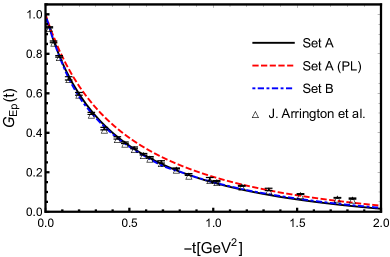
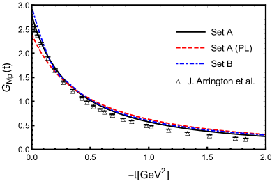
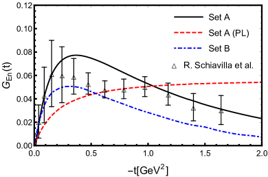
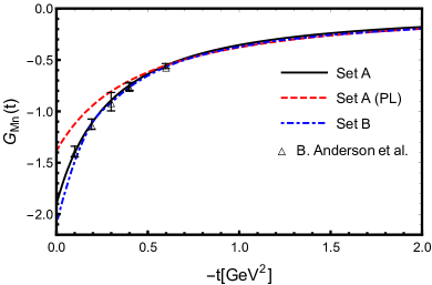
Figure 5: Calculated EMFFs of the proton and the neutron. The black solid and blue dot-dashed curves respectively represent the total EMFFs calculated with the parameters in Set A and Set B, the red dashed curves are those obtained with the Set A parameters but no pion cloud. The results are compared with the data (empty triangle) extracted from the experiments in Ref. [36, 38, 39].

	$\mu_{p}/\mu_{N}$	$\sqrt{\langle r^{2}_{Ep}\rangle}/\text{fm}$	$\sqrt{\langle r^{2}_{Mp}\rangle}/\text{fm}$	$\mu_{n}/\mu_{N}$	$\langle r^{2}_{En}\rangle/\text{fm}^{2}$	$\sqrt{\langle r^{2}_{Mn}\rangle}/\text{fm}$
Set A	2.79	0.89	0.90	-1.90	-0.20	0.95
Set A (PL)	2.42	0.76	0.72	-1.38	-0.06	0.71
Set B	2.96	0.87	0.90	-2.10	-0.14	0.96
PDG [37]	2.79	0.84	0.851$\pm$0.026	-1.91	-0.12	$0.864^{+0.009}_{-0.008}$

Table 3: Electromagnetic properties of the nucleon. The second and fourth rows respectively lists the electromagnetic properties calculated with the Set A and Set B parameters, while the third row presents those with the Set A parameters but no pion cloud.

3.3 GFFs of the nucleon

The numerical results of the GFFs are illustrated in Fig. 6. The GFFs are independent of the charge, and thus those of the proton and the neutron are indistinguishable. The normalization constants employed here are the same as those used during the calculation of the EMFFs to maintain the consistency. However, the momentum-dependent scalar function introduced in Eq. (19) may break the gauge invariance and the Ward-Takahashi identity [18, 40]. As a result, the form factors $G_{E}(t)$ and $\varepsilon_{0}(t)$ cannot be normalized at the same time. It is seen that $\varepsilon_{0}(0)\sim 0.96$ and $\mathcal{J}_{1}(0)\sim 0.50$, which are in close agreement with the normalization condition $\varepsilon_{0}(0)=1$ and $\mathcal{J}_{1}(0)=1/2$. Table 4 lists the mass radius of the nucleon. Comparing with the electromagnetic radii in Tab. 3, the mass radius is slightly smaller, which is consistent with our previous study about the decuplet baryons [25]. The GFFs obtained without the pion cloud effect are illustrated with the red curves in Fig. 6. It is evident that the energy and angular momentum form factors still meet the agreement of the normalization condition, with $\varepsilon_{0}^{PL}(0)\sim 0.95$ and $\mathcal{J}_{1}^{PL}(0)\sim 0.49$, while the D-term $D_{0}^{PL}(0)\sim 0.39$ is about $18\%$ larger. Furthermore, similar with the charge radius, the pion cloud raises the mass radius of the nucleon by about $9\%$.

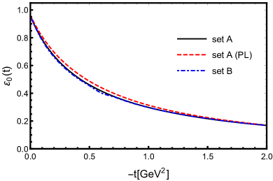
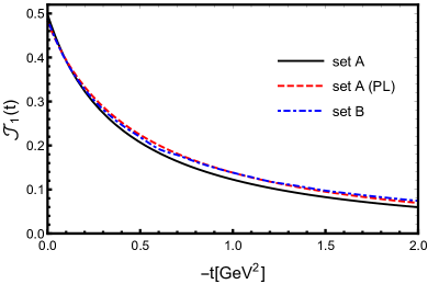
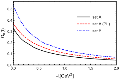
Figure 6: Calculated GFFs of the nucleon. The black solid and blue dot-dashed curves respectively represent the total GFFs calculated with the parameters in Set A and Set B, the red dashed curves stand for those with the Set A parameters but no pion cloud.

	Set A	Set A (PL)	Set B	[10]	[12]	[41]
$\sqrt{\langle r^{2}_{m}\rangle}/\text{fm}^{2}$	0.73	0.67	0.74	0.82	0.82	0.88

Table 4: Calculated mass radii of the nucleon, compared with that evaluated without the pion cloud and the results from the chiral quark-soliton model [10], Skyrme model [12], and $\pi-\rho-\omega$ soliton model [41].

The densities of energy, angular momentum in the $r$-space inside the nucleon can be derived through the Fourier transformation. Refs. [42, 43, 44] suggest that the local density distribution must depend on the size of the wave packet of the system. Furthermore, an additional wave packet is necessary physically and mathematically to guarantee the convergence of the Fourier transformation. Here we simply employ a Gaussian-like wave packet $e^{t/\lambda^{2}}$ [45], where $\lambda$ has the mass dimension and $1/\lambda$ correlates with the size of the hadron. The parameter $\lambda$ may influence the definition of the radius [42, 46]. However, this issue is not a priority in this work. Figure 7 shows the energy and angular momentum densities calculated with Set A parameters, and the densities obtained without the pion cloud are also illustrated. In our previous work on the decuplet baryons [25], we adapted an empirical relationship $\sqrt{\langle r^{2}\rangle_{m}}=\alpha/\lambda$ with $\alpha\sim 4$. With the calculated mass radius $\langle r^{2}\rangle_{m}=0.73\,\text{fm}^{2}$ in Tab. 4, we choose $\lambda=0.92$ GeV during the calculation.

The integrated results of $\mathcal{E}_{0}(r)$ and $\rho_{J}(r)$ over the whole coordinate space could still gives the mass and spin of the nucleon, which satisfies the normalization condition. Comparing the two curves in both panels, the pion cloud depresses the densities in small $r$, and in larger $r$ (approximately when $r>1\,\text{fm}$), the densities with the pion cloud effect are slightly larger. The results indicate that the pion cloud may distract the angular momentum distribution from the origin. As illustrated in Fig. 6, the pion cloud surrounding the quark raises the mass and angular momentum radii, thereby shifting their distribution farther away, which is consistent with our intuitive expectations.

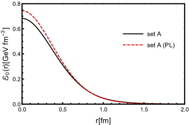
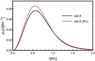
Figure 7: The energy (left panel) and angular momentum (right) densities of the nucleon as the functions of $r$, and the black solid and red dashed curves respectively represent the densities with and without the pion cloud effect.

$D_{0}(t)$, which is believed connecting with the pressure and shear force in the classical physical concept [1], is positive in Fig. 6 with $D_{0}=0.33$. However, it is argued that the D-term should be negative in order to guarantee the stability of the system in Ref. [47]. The sign of the present D-term is consistent with our previous results [24, 25] in the same quark-diquark approach, and with the result of the hydrogen atom [48]. Although the phenomenon of $D_{0}>0$ does not consistent with the arguments in Ref. [47], it still satisfies the von Laue condition $\int^{\infty}_{0}drr^{2}p_{0}(r)=0$ as shown in Fig. 8. Here, we argue that the classical definitions of the pressure and shear force may not be applicable to the relativistic quantum few-body system we are dealing with, because they are derived from the statistical mean in the classical multi-body systems. The hydrogen atom is also a few-body system, so its non-positive D-term is not necessary. A more detailed discussion has been given in our work on $\Omega^{-}$ in Ref. [26].

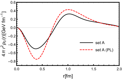
Figure 8: $4\pi r^{2}p_{0}(r)$ as a function of $r$. The areas of the lower part is equal to the upper part, which satisfies the von Laue condition. Due to the positive $D_{0}(t)$, the pressure and the shear force have opposite signs compared to other studies. Nevertheless, as discussed before [26], the pressure and shear force obtained here may differ from the classical definitions.

4 Summary And Discussion

In this work, both the EMFFs and GFFs of the nucleon have been simultaneously calculated with a relativistic covariant quark-diquark model to simplify the structure of the nucleon from a three-body system into a two-body system. An additional scalar function is simply employed to simulate the bound state between the quark and the diquark instead of direct solving the Bethe-Salpeter equation. Furthermore, the pion cloud is taken into consideration to obtain more reasonable results. In this work, it is assumed that the quark is no longer a point-like particle, but a so-called dressed quark coupling with the pion. Considering the quark internal structure, the coupling vertex between the quark and the electromagnetic or the EMT current is modified.

The form factors are calculated with two sets of parameters. The parameters in Set A are determined through fitting the experiment data of the EMFFs, and Set B parameters are adopted from our previous study on $\Delta$ to facilitate our future work on the $N-\Delta$ transition. Given that the nucleon is a spin-1/2 particle, the diquark inside could be regarded as either a scalar or an axialvector one. In our results, the scalar diquark provides larger radii while the introduction of the axialvector diquark could raise the magnetic moments. Furthermore, the spin of the diquark does little influence on the GFFs expect $D_{0}(t)$. Through fitting the experiment data, we choose the mixing angle $\sin^{2}\theta=0.23$, which indicates that the scalar diquark takes a dominant position in the diquark constituent.

The calculated EMFFs are found to be in reasonably agreement with the experiment data and with the results of other theoretical studies. In comparison with the form factors obtained with the point-like quarks, the magnetic form factors of both the proton and the neutron increase significantly. Moreover, the magnitude of the electromagnetic radii, particularly for the neutron, are raised. The transition process between the scalar and axialvector diquark exerts little influence on the electric form factors of the nucleon, but increases the magnitude of the magnetic form factors significantly.

In regard of the GFFs results, the energy and the angular momentum form factors could nearly satisfy the normalization condition. However, the D-term obtained is positive, which is argued to be negative to guarantee the stability of the system. We argue that the classical definitions of the pressure and shear force may not be applicable to the relativistic quantum few-body system, and the positive D-term could still maintain the stability of the system. The pion cloud effect on the energy and the angular momentum form factors is negligible, while it results in a reduction in $D_{0}(t)$, which is related to the internal forces of the nucleon. Similar with the EMFFs, the mass radius of the nucleon is raised by the pion cloud, and the obtained mass radius is smaller than the charge and magnetic radii of the proton. The energy and the angular momentum densities in the coordinate space are obtained through the Fourier transformation. The densities are depressed by the pion cloud in the region of small $r$, because the pion cloud surrounding the quark could distract the mass away from the origin.

With the nucleon form factors obtained, our future studies will be applied to the $N-\Delta$ transition and the deuteron composed of a proton and a neutron. In our previous papers [25, 24], the pion cloud effect was not considered. It is expected that the pion cloud effect on the properties of the decuplet baryons, especially $\Delta$, will be further discussed in our further studies.

References

- [1] Maxim V. Polyakov and Peter Schweitzer. Forces inside hadrons: Pressure, surface tension, mechanical radius, and all that. International Journal of Modern Physics A, 33(26):1830025, 2018.
- [2] V. Punjabi, C. F. Perdrisat, M. K. Jones, E. J. Brash, and C. E. Carlson. The structure of the nucleon: Elastic electromagnetic form factors. The European Physical Journal A, 51(7):79, 2015.
- [3] Xiang-Dong Ji. Off forward parton distributions. J. Phys. G, 24:1181–1205, 1998.
- [4] M. Diehl. Generalized parton distributions. Phys. Rept., 388:41–277, 2003.
- [5] Maxim V. Polyakov and Bao-Dong Sun. Gravitational form factors of a spin one particle. Phys. Rev. D, 100:036003, 2019.
- [6] Bao-Dong Sun and Yu-Bing Dong. Gravitational form factors of meson with a light-cone constituent quark model. Phys. Rev. D, 101:096008, 2020.
- [7] V. D. Burkert, L. Elouadrhiri, and F. X. Girod. The pressure distribution inside the proton. Nature, 557(7705):396–399, 2018.
- [8] N. Mathur, S. J. Dong, K. F. Liu, L. Mankiewicz, and N. C. Mukhopadhyay. Quark orbital angular momentum from lattice QCD. Phys. Rev. D, 62:114504, 2000.
- [9] Ph. Hagler et al. Nucleon Generalized Parton Distributions from Full Lattice QCD. Phys. Rev. D, 77:094502, 2008.
- [10] K. Goeke, J. Grabis, J. Ossmann, M. V. Polyakov, P. Schweitzer, A. Silva, and D. Urbano. Nucleon form-factors of the energy momentum tensor in the chiral quark-soliton model. Physical Review D, 75(9):094021, 2007. arXiv:hep-ph/0702030.
- [11] June-Young Kim and Hyun-Chul Kim. Energy-momentum tensor of the nucleon on the light front: Abel tomography case. Phys. Rev. D, 104:074019, Oct 2021.
- [12] Hyun-Chul Kim, Peter Schweitzer, and Ulugbek Yakhshiev. Energy–momentum tensor form factors of the nucleon in nuclear matter. Physics Letters B, 718(2):625–631, 2012.
- [13] Poonam Choudhary, Bheemsehan Gurjar, Dipankar Chakrabarti, and Asmita Mukherjee. Gravitational form factors and mechanical properties of the proton: Connections between distributions in 2D and 3D. Phys. Rev. D, 106(7):076004, 2022.
- [14] Cédric Lorcé, Peter Schweitzer, and Kemal Tezgin. 2d energy-momentum tensor distributions of nucleon in a large- quark model from ultrarelativistic to nonrelativistic limit. Phys. Rev. D, 106:014012, 2022.
- [15] K. Azizi and U. Özdem. Nucleon’s energy–momentum tensor form factors in light-cone QCD. Eur. Phys. J. C, 80(2):104, 2020.
- [16] I. V. Anikin. Gravitational form factors within light-cone sum rules at leading order. Phys. Rev. D, 99:094026, 2019.
- [17] V. D. Burkert, L. Elouadrhiri, F. X. Girod, C. Lorcé, P. Schweitzer, and P. E. Shanahan. Colloquium: Gravitational form factors of the proton. Rev. Mod. Phys., 95(4):041002, 2023.
- [18] Wojciech Broniowski and Enrique Ruiz Arriola. Gravitational and higher-order form factors of the pion in chiral quark models. Physical Review D, 78(9), 2008.
- [19] S. Kumano, Qin-Tao Song, and O. V. Teryaev. Hadron tomography by generalized distribution amplitudes in the pion-pair production process and gravitational form factors for pion. Phys. Rev. D, 97:014020, 2018.
- [20] T. M. Aliev, T. Barakat, and K. Şimşek. Gravitational formfactors of the , , and mesons in the light-cone qcd sum rules. Phys. Rev. D, 103:054001, 2021.
- [21] Bao-Dong Sun and Yu-Bing Dong. meson unpolarized generalized parton distributions with a light-front constituent quark model. Phys. Rev. D, 96:036019, 2017.
- [22] Adam Freese and Ian C. Cloët. Gravitational form factors of light mesons. Phys. Rev. C, 100:015201, 2019.
- [23] June-Young Kim and Bao-Dong Sun. Gravitational form factors of a baryon with spin-3/2. Eur. Phys. J. C, 81(1):85, 2021.
- [24] Dongyan Fu, Bao-Dong Sun, and Yubing Dong. Electromagnetic and gravitational form factors of resonance in a covariant quark-diquark approach. Phys. Rev. D, 105:096002, 2022.
- [25] JiaQi Wang, Dongyan Fu, and Yubing Dong. Form factors of decuplet baryons in a covariant quark–diquark approach. The European Physical Journal C, 84(1):79, 2024.
- [26] Dongyan Fu, JiaQi Wang, and Yubing Dong. Form factors of in a covariant quark-diquark approach. Phys. Rev. D, 108:076023, 2023.
- [27] Anthony William Thomas, S. Theberge, and Gerald A. Miller. The Cloudy Bag Model of the Nucleon. Phys. Rev. D, 24:216, 1981.
- [28] Ian C. Cloët, Wolfgang Bentz, and Anthony W. Thomas. Role of diquark correlations and the pion cloud in nucleon elastic form factors. Physical Review C, 90(4):045202, 2014.
- [29] Sabrina Cotogno, Cédric Lorcé, Peter Lowdon, and Manuel Morales. Covariant multipole expansion of local currents for massive states of any spin. Physical Review D, 101(5):056016, 2020.
- [30] F. J. Ernst, R. G. Sachs, and K. C. Wali. Electromagnetic form factors of the nucleon. Phys. Rev., 119:1105–1114, 1960.
- [31] Bo-Qiang Ma, Di Qing, and Ivan Schmidt. Electromagnetic form-factors of nucleons in a light cone diquark model. Phys. Rev. C, 65:035205, 2002.
- [32] Michael D. Scadron. Covariant propagators and vertex functions for any spin. Physical Review, 165(5):1640–1647, 1968.
- [33] T. Frederico, E. Pace, B. Pasquini, and G. Salmè. Pion generalized parton distributions with covariant and light-front constituent quark models. Phys. Rev. D, 80:054021, 2009.
- [34] H. Meyer. The nucleon as a relativistic quark-diquark bound state with an exchange potential. Physics Letters B, 337(1–2):37–42, 1994.
- [35] Cédric Lorcé. New explicit expressions for dirac bilinears. Phys. Rev. D, 97:016005, Jan 2018.
- [36] J. Arrington, W. Melnitchouk, and J. A. Tjon. Global analysis of proton elastic form factor data with two-photon exchange corrections. Phys. Rev. C, 76:035205, Sep 2007.
- [37] S. Navas et al. Review of particle physics. Phys. Rev. D, 110(3):030001, 2024.
- [38] R. Schiavilla and I. Sick. Neutron charge form-factor at large . Phys. Rev. C, 64:041002, 2001.
- [39] B. Anderson et al. Extraction of the Neutron Magnetic Form Factor from Quasi-elastic at Q2 = 0.1 - 0.6 (GeV/c)2. Phys. Rev. C, 75:034003, 2007.
- [40] R.M. Davidson and Ruiz Arriola E. Structure functions of pseudoscalar mesons in the su(3) njl model. Physics Letters B, 348(1):163–169, 1995.
- [41] Ju-Hyun Jung, Ulugbek Yakhshiev, Hyun-Chul Kim, and Peter Schweitzer. In-medium modified energy-momentum tensor form factors of the nucleon within the framework of a -- soliton model. Phys. Rev. D, 89(11):114021, 2014.
- [42] E. Epelbaum, J. Gegelia, N. Lange, U. G. Meißner, and M. V. Polyakov. Definition of Local Spatial Densities in Hadrons. Phys. Rev. Lett., 129(1):012001, 2022.
- [43] M. Diehl. Generalized parton distributions in impact parameter space. The European Physical Journal C, 25(2):223–232, 2002.
- [44] Adam Freese and Gerald A. Miller. Unified formalism for electromagnetic and gravitational probes: Densities. Physical Review D, 105(1):014003, 2022.
- [45] Tomomi Ishikawa, LuChang Jin, Huey-Wen Lin, Andreas Schäfer, Yi-Bo Yang, Jian-Hui Zhang, and Yong Zhao. Gaussian-weighted parton quasi-distribution (Lattice Parton Physics Project (LP3)). Sci. China Phys. Mech. Astron., 62(9):991021, 2019.
- [46] H. Alharazin, B. D. Sun, E. Epelbaum, J. Gegelia, and U. G. Meißner. Local spatial densities for composite spin-3/2 systems. JHEP, 02:163, 2023.
- [47] Irina A. Perevalova, Maxim V. Polyakov, and Peter Schweitzer. Lhcb pentaquarks as a baryon- bound state: Prediction of isospin- pentaquarks with hidden charm. Phys. Rev. D, 94:054024, 2016.
- [48] Xiangdong Ji and Yizhuang Liu. Momentum-Current Gravitational Multipoles of Hadrons. Phys. Rev. D, 106(3):034028, 2022.