Straightness of Rectified Flow: A Theoretical Insight into Wasserstein Convergence

Abstract

Diffusion models have emerged as a powerful tool for image generation and denoising. Typically, generative models learn a trajectory between the starting noise distribution and the target data distribution. Recently Liu et al. (2023b) designed a novel alternative generative model Rectified Flow (RF), which aims to learn straight flow trajectories from noise to data using a sequence of convex optimization problems with close ties to optimal transport. If the trajectory is curved, one must use many Euler discretization steps or novel strategies, such as exponential integrators, to achieve a satisfactory generation quality. In contrast, RF has been shown to theoretically straighten the trajectory through successive rectifications, reducing the number of function evaluations (NFEs) while sampling. It has also been shown empirically that RF may improve the straightness in two rectifications if one can solve the underlying optimization problem within a sufficiently small error. In this paper, we make two key theoretical contributions: 1) we provide the first theoretical analysis of the Wasserstein distance between the sampling distribution of RF and the target distribution. Our error rate is characterized by the number of discretization steps and a new formulation of straightness stronger than that in the original work. 2) In line with the previous empirical findings, we show that, for a rectified flow from a Gaussian to a mixture of two Gaussians, two rectifications are sufficient to achieve a straight flow. Additionally, we also present empirical results on both simulated and real datasets to validate our theoretical findings.

1 Introduction

In recent years, diffusion models have achieved impressive performance across different multi-modal tasks including image (Ho et al., 2022b; Balaji et al., 2022; Rombach et al., 2022), video (Ho et al., 2022a; c; Luo et al., 2023; Wang et al., 2024; Zhou et al., 2022), and audio (Huang et al., 2023; Kong et al., 2020; Liu et al., 2023a; Ruan et al., 2023) generation that leverages the score-based generative model (SGM) framework (Sohl-Dickstein et al., 2015; Ho et al., 2020), which is a key component of large-scale generative models such as DALL-E 2 (Ramesh et al., 2022). The main idea in this framework is to gradually perturb the data according to a pre-defined diffusion process, and then to learn the reverse process for sample generation. Despite its success, the SGM framework incurs significant computational costs because it requires numerous inference steps to generate high-quality samples. The primary reason is that SGM generates sub-optimal or complicated flow trajectories that make the sampling step expensive. An alternative approach to sampling in diffusion models involves solving the corresponding probability-flow ordinary differential equations (ODEs) (Song et al., 2020b; 2023). This has led to the development of faster samplers, such as DDIM (Song et al., 2020a), DPM solvers (Lu et al., 2022; Zheng et al., 2023), DEIS (Zhang & Chen, 2022), and Genie (Dockhorn et al., 2022). However, these methods still require dozens of inference steps to produce satisfactory results.

To alleviate this computational bottleneck in the sampling stage, Liu et al. (2023b) recently proposed rectified flow, which aims to efficiently sample from the target distribution by iteratively learning the straight flow trajectories. To elucidate further, rectified flow starts from a potentially curved flow model, similar to DDIM (Song et al., 2020a) or other flow-based models (Lipman et al., 2022; Albergo & Vanden-Eijnden, 2022; Albergo et al., 2023), that transports the noise distribution to the target distribution, and then applies the reflow procedure to straighten the trajectories of the flow, thereby reducing the transport cost (Liu, 2022; Shaul et al., 2023b). Recent experimental studies in Liu et al. (2024; 2023b) have demonstrated that rectified flow can achieve high-quality image generation within one or two steps just after 2-rectification procedures. Lee et al. (2024) recently proposed an improved training routine for rectified flow and also achieved impressive results just after 2-rectification procedures. However, despite the computational advancements, a theoretical understanding of the convergence rate of rectified flow to the true data distribution and the effect of straightness on its computational complexity remains elusive. In this paper, we investigate these issues and make the following contributions.

• Wasserstein convergence and effect of straightness: We establish a new bound for the 2-Wasserstein distance between the sampled data distribution in rectified flow and the true target distribution that mainly depends on the estimation error of the velocity (or drift) function and the discretization error induced by the Euler discretization scheme. We also show that the discretization error is proportional to novel straightness parameters of the flow that takes small values for near straight flows. Therefore, our result explains the rationale behind the sufficiency of fewer discretization steps in the sampling stage under near-straight flows with rigorous theoretical underpinning.

• Analysis of rectified flow in Gaussian mixtures: In addition to deriving general bounds for Wasserstein convergence, we conduct a detailed analysis of simple yet previously unexplored models where straight flows are provably achievable through rectification. Empirical observations, both in simulations and real-world data, have shown that only a few iterations of the procedure are often sufficient to produce straight flows (REFs). However, there is limited theoretical understanding of the types of distributions that exhibit this property. To address this gap, we study the geometry of rectified flow between a standard Gaussian and a 2-mixture of Gaussians (and simple Gaussian) in $\mathbb{R}^{d}$, demonstrating that 2-rectifications are sufficient to achieve straight flows. We also extend this analysis to the symmetric case of 2-mixture to 2-mixture Gaussian flow in $\mathbb{R}^{2}$, establishing the straightness of the 2-rectified flow, a property observed empirically and conjectured in Lee et al. (2024).

The rest of the paper is organized as follows: Section 2 provides some background on optimal transport and its connection with rectified flow. In Section 3, we present the main convergence results for the continuous time and discretized rectified flow under the 2-Wasserstein metric. We also introduce novel straightness parameters and study their effect on the convergence rate. Section 4 focuses on the geometry of 1-rectified flow for some Gaussian mixture models. In these special cases, we show that two rectifications are sufficient to obtain a straight flow. Finally, we present supporting simulated and real data experiments in Section 5 to empirically validate our theoretical findings.

Notation. Let $\mathbb{R}$ denote the set of real numbers. We denote by $\mathbb{R}^{d}$ the $d$-dimensional Euclidean space, and for a vector $x\in\mathbb{R}^{d}$, we denote by $\left\|{x}\right\|_{2}$ the $\ell_{2}$-norm of $x$. We use $I_{d}$ to denote the $d$-dimensional identity matrix. For a positive integer $K$, denote by $[K]$ the set $\{1,2,\ldots,K\}$.

Regarding random variables and distributions, for a random variable $X$ we denote by $\text{Law}(X)$ the probability distribution (or measure) of $X$. We write $X\sim\rho$ to denote $\rho=\text{Law}(X)$. Moreover, for an absolutely continuous probability distribution $\rho$ with respect to the Lebesgue measure $\lambda$ over $\mathbb{R}^{d}$, we denote by $\frac{d\rho}{d\lambda}$ the Radon-Nikodym derivative of $\rho$ with respect to $\lambda$, i.e., the density of $X$ with respect to $\lambda$ is $\xi:=\frac{d\rho}{d\lambda}$. For two distributions $\rho_{1}$ and $\rho_{2}$, we use $W_{2}(\rho_{1},\rho_{2})$ to denote the 2-Wasserstein distance between $\rho_{1}$ and $\rho_{2}$. We denote by $N(0,I_{d})$ the standard gaussian distribution in $\mathbb{R}^{d}$.

For a continuous and differentiable path $\{x_{t}\}_{t\in[0,1]}\subset\mathbb{R}^{d}$ and time varying functions $f_{t}:\mathbb{R}^{d}\to\mathbb{R}^{m}$, we denote by $\dot{f}_{t}(x_{t})$ the time derivative of $f_{t}(x_{t})$, i.e., $\dot{f}_{t}(x_{t})=\frac{df_{t}(x_{t})}{dt}$. Similarly, we use $\ddot{f}_{t}(x_{t})$ to denote $\frac{d^{2}f_{t}(x_{t})}{dt^{2}}$. For a vector field $v:\mathbb{R}^{d}\to\mathbb{R}^{d}$, we let $\nabla\cdot v$ be its divergence.

Throughout the paper, we will use standard big-Oh (respectively big-Omega) notation. In detail, for a sequence $\{a_{n}\}$ of real numbers and a sequence $\{b_{n}\}$ of positive numbers, $a_{n}=O(b_{n})$ (respectively $a_{n}=\Omega(b_{n})$) signifies that there exists a universal constant $C>0$, such that $|a_{n}|\leq Cb_{n}$ (respectively $|a_{n}|\geq Cb_{n}$) for all $n\in\mathbb{N}$.

2 Background and Preliminaries

2.1 Optimal Transport

The optimal transport (OT) problem was first formulated as the Monge problem (Monge, 1781) given by:

$$\inf_{\mathcal{T}}\mathbb{E}\left[{{c(\mathcal{T}(X_{0})-X_{0})}}\right]\quad\text{s.t.}\quad\text{Law}(\mathcal{T}(X_{0}))=\rho_{1},\quad\text{Law}(X_{0})=\rho_{0},\quad$$

where the the infimum is taken over deterministic couplings $(X_{0},X_{1})$ where $X_{1}=\mathcal{T}(X_{0})$ for $\mathcal{T}:\mathbb{R}^{d}\to\mathbb{R}^{d}$ to minimize the $c$-transport cost. The Monge problem was relaxed by Kantorovich (Kantorovich, 1958) and the Monge-Kantorovich (MK) problem allowed for all (deterministic and stochastic) couplings $(X_{0},X_{1})$ with marginal laws $\rho_{0}$ and $\rho_{1}$ respectively. However, it is well-known that if $\rho_{0}$ is an absolutely continuous probability measure on $\mathbb{R}^{d}$, both problems have the same optimal coupling that is deterministic, and hence, the optimization could be restricted only to the set of deterministic mappings $\mathcal{T}$. We consider an equivalent dynamic formulation of the Monge and MK problems as finding a continuous-time process $\left\{{X_{t}}\right\}_{t\in[0,1]}$ from the collection of all smooth interpolants $\mathcal{X}$ such that $X_{0}\sim\rho_{0}$ and $X_{1}\sim\rho_{1}$. For convex cost functions $c$, Jensens’s inequality gives that

$$\mathbb{E}\left[{{c(X_{1}-X_{0})}}\right] =\mathbb{E}\left[{{c\left({\int_{0}^{1}\dot{X}_{t}dt}\right)}}\right]=\inf_{\left\{{X_{t}}\right\}_{t\in[0,1]}\in\mathcal{X}}\mathbb{E}\left[{{\int_{0}^{1}c\left({\dot{X}_{t}}\right)dt}}\right]$$

where the infimum is indeed achieved when $X_{t}=tX_{1}+(1-t)X_{0}$, also known as the displacement interpolant, which forms a geodesic in the Wasserstein space (see McCann (1997)). When we restrict the processes to those induced by the ODEs of the form $dX_{t}=v_{t}(X_{t})dt$. The Lebesgue density of $X_{t}$, denoted by $\xi_{t}$, follows the continuity equation (also known as the Fokker-Planck equation) given by $\frac{\partial\xi_{t}}{\partial t}+\nabla\cdot(v_{t}\xi_{t})=0,$ and the Monge problem can be recast as

$$\inf_{v,\mathcal{X}}\mathbb{E}\left[{{\int_{0}^{1}c\left({v_{t}(X_{t})}\right)dt}}\right],\quad\text{s.t.}\quad\frac{\partial\xi_{t}}{\partial t}+\nabla\cdot(v_{t}\xi_{t})=0,\quad\xi_{0}=\frac{d\rho_{0}}{d\lambda}\quad\text{and}\quad\xi_{1}=\frac{d\rho_{1}}{d\lambda}.$$

However, the dynamic formulation outlined above is challenging to solve in practice. When the cost function $c=\|\cdot\|^{2}$, this corresponds exactly to the kinetic energy objective introduced by Shaul et al. (2023a), who demonstrates that the displacement interpolant minimizes the kinetic energy of the flow, resulting in straight-line flow paths. Additionally, Liu (2022) shows that Rectified Flow, which iteratively learns the drift function $v_{t}$ for the displacement interpolant, simplifies this complex problem into a series of least-squares optimization tasks. With each iteration of Rectified Flow, the transport cost is reduced for all convex cost functions $c$.

2.2 Rectified Flow

In this section, we briefly introduce the basics of Rectified flow Liu et al. (2023b); Liu (2022), a generative model that transitions between two distributions $\rho_{0}$ and $\rho_{1}$ by solving ordinary differential equations (ODEs). Let $\rho_{\rm{data}}:=\rho_{1}=\text{Law}(X_{1})$ be the target data distribution on $\mathbb{R}^{d}$ and the linear-interpolation process be given by

$$X_{t}=tX_{1}+(1-t)X_{0},\quad 0\leq t\leq 1$$

where $\rho_{t}=\text{Law}(X_{t})$ (with a slight abuse of notation, we also use it to refer to the density function if it exists) and the starting distribution $\rho_{0}$ is typically a standard Gaussian or any other distribution that is easy to sample from. The training proceeds by optimizing the following objective to learn the drift function $v:\mathbb{R}^{d}\times[0,1]\rightarrow\mathbb{R}^{d}$ as follows:

$$v ={\arg\min}_{f}\int\mathbb{E}\left[{{\|\dot{X}_{t}-f(X_{t},t)\|_{2}^{2}}}\right]dt={\arg\min}_{f}\int\mathbb{E}\left[{{\left\|{(X_{1}-X_{0})-f(X_{t},t)}\right\|_{2}^{2}}}\right]dt,$$ (1)

where, in practice, the initial coupling is usually an independent coupling, i.e., $(X_{0},X_{1})\sim\rho_{0}\times\rho_{1}$. The MMSE objective in (1) is minimized at:

$$v_{t}(x):=v(x,t) =\mathbb{E}\left[{{\dot{X}_{t}\mid X_{t}=x}}\right]=\mathbb{E}\left[{{X_{1}-X_{0}\mid X_{t}=x}}\right]\quad\hfill\text{for }t\in(0,1).$$ (2)

For sampling, Liu et al. (2023b) show that the ODE

$$dZ_{t}=v_{t}(Z_{t})\ dt,\quad\hfill\text{where }Z_{0}\sim\rho_{0}$$ (3)

yields the same marginal distribution as $X_{t}$ for any $t,$ i.e., $\text{Law}(Z_{t})=\text{Law}(X_{t})=\rho_{t},$ owing to the identical Fokker-Planck equations. We call $\mathcal{Z}=\left\{{Z_{t}}\right\}_{t\in[0,1]}$ the rectified flow of the coupling $(X_{0},X_{1})$, denoted as $\mathcal{Z}=\texttt{Rectflow}\left({(X_{0},X_{1})}\right)$, and $(Z_{0},Z_{1})$ the rectified coupling, denoted as $(Z_{0},Z_{1})=\texttt{Rectify}\left({(X_{0},X_{1})}\right)$.

The uniform lipschitzness of the drift function $v_{t}$ for all $t\in[0,1]$ is a sufficient condition for the rectified flow $\mathcal{Z}$ to be unique (Murray & Miller, 2013, Theorem 1). Hence, the Rectflow procedure rewires the trajectories of the linear interpolation process such that no two paths, corresponding to different initial conditions, intersect at the same time. After solving the ODE (3), one can also apply another Rectflow procedure, also called Reflow or the 2-Rectified flow, to the coupling $(Z_{0},Z_{1})$ by learning the drift function

$$v^{(2)}_{t}(Z^{(2)}_{t})=\mathbb{E}\left[{{Z_{1}-Z_{0}\mid tZ_{1}+(1-t)Z_{0}=Z^{(2)}_{t}}}\right].$$

This procedure can be done recursively to get a $K$-rectified flow. Liu (2022) shows that $K$-Rectified flow couplings are straight in the limit of $K\to\infty.$ We give the formal definition of straightness below.

Definition 2.1.

(Straight coupling and flow) A coupling $(X_{0},X_{1})$ is called straight or fully rectified when its linear interpolation paths do not intersect, or equivalently, letting $t\sim\text{Unif}\left({[0,1]}\right)$, $\mathbb{E}\left[{{X_{1}-X_{0}\mid tX_{1}+(1-t)X_{0}}}\right]=X_{1}-X_{0}$, almost surely.

Moreover, for a straight coupling $(X_{0},X_{1})$, the corresponding rectified flow $\mathcal{Z}=\texttt{Rectflow}\left({(X_{0},X_{1})}\right)$ has straight line trajectories, and $(X_{0},X_{1})\overset{d}{=}(Z_{0},Z_{1})=\texttt{Rectify}\left({(X_{0},X_{1})}\right)$, i.e., they both have the same joint distribution. A flow that satisfies these properties is called a straight flow.

Straight flows are especially appealing because, in practice, solving the ODE (3) analytically is rarely feasible, necessitating the use of discretization schemes for numerical solutions. However, for straight flows, the trajectories follow straight lines, allowing for closed-form solutions without the need for iterative numerical solvers, which significantly accelerates the sampling process.

Moreover, in practice, one is usually given samples from $\rho_{\rm{data}}$, and the drift function is estimated by empirically minimizing the objective in (1) over a large and expressive function class $\mathcal{F}$ (for example, the class of neural networks) and replaced in (3). Consequently, the estimate $\widehat{v}_{t}$ is used to obtain the following sampling ODE:

$$d\tilde{Y}_{t}=\widehat{v}_{t}(\tilde{Y}_{t})\,dt,\quad\hfill\text{where }\tilde{Y}_{0}\sim N(0,I_{d})$$ (4)

When the solution to the ODE (4) is not analytically available, one must rely on discretization schemes. As proposed in Liu et al. (2023b), we apply the Euler discretization of the ODE to obtain our final sample estimates as mentioned below:

$$\widehat{Y}_{t_{i}}=\widehat{Y}_{t_{i-1}}+\widehat{v}_{t_{i-1}}(\widehat{Y}_{t_{i-1}})(t_{i}-t_{i-1}),\quad\hfill\text{for }i\in[T],$$ (5)

where the ODE is discretized into $T$ uniformly spaced steps, with $t_{i}=i/T$. The final sample estimate, $\widehat{Y}_{1}$, follows the distribution $\widehat{\rho}_{\rm{data}}:=\text{Law}(\widehat{Y}_{1})$.

3 Main results on Wasserstein convergence

3.1 Continuous time Wasserstein convergence

In this section, we study the convergence error rate of the final estimated distribution of the rectified flow. In particular, we establish error rates in the 2-Wasserstein distance for the estimated distributions procured through the approximate ODE flow (4). To this end, we make some useful assumptions on the drift function and its estimate that are necessary for establishing error bounds:

Assumption 3.1.

We assume that

1. (Estimation error) There exists ${\varepsilon_{\rm vl}}\geq 0$ such that the following holds:

   $$\mathbb{E}_{X_{t_{i}}\sim\rho_{t_{i}}}{\left\|{v_{t_{i}}(X_{t_{i}})-\widehat{v}_{t_{i}}(X_{t_{i}})}\right\|_{2}^{2}}\leq{\varepsilon^{2}_{\rm vl}}\quad\text{for all $0\leq i\leq T$}.$$

2. (Lipschitz condition) The drift function $\widehat{v}_{t}$ satisfies $\left|{\widehat{v}_{t}(x)-\widehat{v}_{t}(y)}\right|\leq\widehat{L}\left\|{x-y}\right\|_{2}$ for some $\widehat{L}>0$.

Assumption 3.1(a) tells that $\widehat{v}_{t}$ is a reasonable approximation of the original drift function $v_{t}$ for all the time points $t\in\{t_{i}\}_{i\in[T]}$. Such assumptions are standard in diffusion model literature (Gupta et al., 2024; Li et al., 2024b; a; Chen et al., 2023), and it is indeed necessary to establish a reasonable bound on the error rate. Assumption 3.1(b) is a standard Lipschitz assumption on the estimated drift function $\widehat{v}_{t}$. In literature concerning the score-based diffusion models and flow-based models, similar Lipschitzness (and one-sided Lipschitzness) assumptions on the estimated score functions of $\{X_{t_{i}}\}_{i\in[T]}$ are common (Chen et al., 2023; Kwon et al., 2022; Li et al., 2024b; Pedrotti et al., 2024; Boffi et al., 2024) requirement for theoretical analysis. In fact, $\widehat{v}$ is typically given by a neural network, which corresponds to a Lipschitz function for most practical activations. Moreover, in the context of rectified flow or flow-based generative models, the lipschitzness condition on the true drift function $v_{t}$ is particularly an important requirement for the existence and uniqueness of the solution of the ODE (3) (Liu et al., 2023b; Boffi et al., 2024). Therefore, it is pragmatic to consider a class of neural networks that satisfies the Lipschitzness property for the training procedure.

Now, we present our first theorem which bounds the error between the actual data distribution $\widehat{\rho}_{\rm{data}}$ and the estimated distribution by following the exact ODE (4).

Theorem 3.2.

Let the condition of Assumption 3.1(b) hold, and also assume that $\rho_{1}$ is absolutely continuous with respect to the Lebesgue measure in $\mathbb{R}^{d}$. Also, write $b(t)=\mathbb{E}_{X_{t}\sim\rho_{t}}\|v_{t}(X_{t})-\widehat{v}_{t}(X_{t})\|_{2}^{2}$ for $t\in[0,1]$, and $\tilde{\rho}_{1}$ be the distribution of $\tilde{Y}_{1}$. Then we have

$$W_{2}^{2}(\tilde{\rho}_{1},\rho_{1})\leq e^{1+2\widehat{L}}\int_{0}^{1}b(t)\;dt.$$

The bound displayed in Theorem 3.2 is indeed very similar to the bounds obtained in Kwon et al. (2022); Pedrotti et al. (2024); Boffi et al. (2024), i.e., the bound essentially depends on the estimation error $b(t)$ for all $t\in[0,1]$. If there exists and $\varepsilon>0$ such that $\sup_{t\in[0,1]}b(t)\leq\varepsilon^{2}$, then we have the bound on the 2-Wasserstein to be of the order $O(\varepsilon^{2})$. However, the requirement on $b(t)$ is much more stringent than the requirement in Assumption 3.1(a) which only requires the control on estimation error corresponding to only the discretized time points $\{t_{i}\}_{i=0}^{T}$. It is also worth mentioning that the Lipschitzness assumption on $\widehat{v}$ can be relaxed to the on-side Lipschitzness condition, i.e., if we have

$$\left\langle\widehat{v}_{t}(x)-\widehat{v}_{t}(y),x-y\right\rangle\leq\widehat{L}\left\|{x-y}\right\|_{2}^{2}\quad\text{for all $t\in[0,1]$},$$

the result of the above theorem also holds true. Moreover, in this case, $\widehat{L}$ may not be necessarily non-negative as required in Assumption 3.1(b). Furthermore, unlike Chen et al. (2023); Gupta et al. (2024), we do not require any second-moment or sub-Gaussian assumption on $X_{t}$ to establish the above bound in Theorem 3.2.

Remark 1.

The absolute continuity requirement in Theorem 3.2 can be relaxed. If the density of $\rho_{1}$ does not exist, then once can convolve $X$ with an independent noise $W_{\eta}\sim N(0,\eta I_{d})$ for a very small $\eta>0$, and consider the mollified distribution $\rho_{1}^{\eta}:=\text{Law}(X+W_{\eta})$ as the target distribution. Note that $\rho_{1}^{\eta}$ is absolutely continuous and satisfies $W_{2}^{2}(\rho_{1}^{\eta},\rho_{1})\leq\eta^{2}d$. Therefore, under the condition of Theorem 3.2, and using triangle inequality we have

$$W_{2}^{2}(\tilde{\rho}_{1},\rho_{1})\lesssim\eta^{2}d+e^{1+2\widehat{L}}\int_{0}^{1}b(t)\;dt.$$

3.2 Straightness and Wasserstein convergence of discretized flow

In this section, we introduce the notion for straightness of the discretized flow (5), and study its effect on the Wasserstein convergence error rate between true data distribution $\rho_{1}$ and the sampled data distribution $\widehat{\rho}_{\rm{data}}$. As we will see in the subsequent discussion, the straightness parameter of the ODE flow (3) plays an imperative role in the error rate, and our analysis shows that a more straight flow requires fewer discretization steps to achieve a reasonable error bound.

New quantifiers for straightness of the flow. We begin by recalling the ODE flow (3):

$$dZ_{t}=v_{t}(Z_{t})dt,\quad Z_{0}\sim N(0,I_{d}).$$

Also, consider the curve $\alpha(t):=(t,Z_{t})$. The straightness of a twice-differential parametric curve is closely related to the curvature of the curve at the points $\{(t,Z_{t})\}_{t\in[0,1]}$. In fact, the curvature of $\alpha$ at time $t$ is measured by the rate of change of tangent vector $\dot{\alpha}(t)=(1,v_{t}(Z_{t}))$, which is essentially the acceleration of the particle at time $t$. To elaborate, let us consider a couple of simple examples of curves (without randomness):

• Straight line: Consider the curve $\alpha(t)=(t,t)$ for $0\leq t\leq 1$. The magnitude of the instantaneous acceleration is $\left\|{\ddot{\alpha}(t)}\right\|_{2}=0$. This leads to the fact that $\alpha(t)$ has no curvature, i.e., it is straight.

• Circle: Consider the curve $\alpha(t)=(\sin t,\cos t)$ for $0\leq t\leq 1$. In this case, the magnitude of the instantaneous acceleration is $\left\|{\ddot{\alpha}(t)}\right\|_{2}=1$. This shows that $\alpha(t)$ has curvature, i.e., it is not straight.

The above discussion motivates us to define two key quantities to measure the straightness of the flow $\mathcal{Z}$:

Definition 3.3.

Let $\mathcal{Z}=\{Z_{t}\}_{t\in[0,1]}$ be twice-differentiable flow following the ODE (3).

1. The average straightness (AS) parameter of $\mathcal{Z}$ is defined as

   $$\gamma_{1}(\mathcal{Z}):=\int_{0}^{1}\mathbb{E}\left\|{\dot{v}_{t}(Z_{t})}\right\|_{2}^{2}\;dt.$$

2. Let $0=t_{0}<t_{1}<\ldots<t_{T}=1$ be a partition of $[0,1]$ into $T$ intervals of equal length. The piece-wise straightness (PWS) parameter of the flow $\mathcal{Z}$ is defined as

   $$\gamma_{2,T}(\mathcal{Z}):=\max_{i\in[T]}\frac{1}{t_{i}-t_{i-1}}\int_{t_{i-1}}^{t_{i}}\mathbb{E}\left\|{\dot{v}_{t}(Z_{t})}\right\|_{2}^{2}\;dt.$$

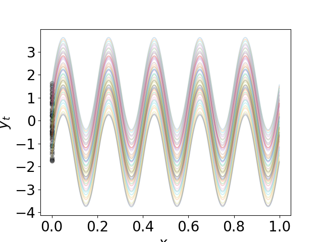
(a) $N=5$

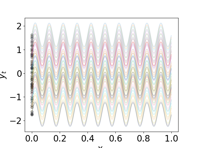
(b) $N=10$

Figure 1: Flow of $Z_{t}=Z_{0}+(t,50N^{-2}\sin(2\pi Nt))^{\top}$ for different choices of $N$.

The quantity $\gamma_{1}(\mathcal{Z})$ essentially captures the average straightness of the flow along the time $t\in[0,1]$. On the other hand, $\gamma_{2,T}(\mathcal{Z})$ captures the degree of straightness of $\mathcal{Z}$ for every interval $[t_{i-1},t_{t}]$ for all $i\in[T]$. Therefore, $\gamma_{2,T}(\mathcal{Z})$ captures a somewhat more stringent notion of straightness. In addition, a small value of $\gamma_{1}(\mathcal{Z})$ or $\gamma_{2,T}(\mathcal{Z})$ indicates that the flow is close to perfect straightness. In fact, $\gamma_{1}(\mathcal{Z})=0$ or $\gamma_{2,T}(\mathcal{Z})=0$ implies that the flow $\mathcal{Z}$ is a straight flow in the sense of Definition 2.1. To formally state the claim, we recall the quantity introduced in Liu et al. (2023b) to measure the degree of straightness of the flow $\mathcal{Z}$:

$$S(\mathcal{Z}):=\int_{0}^{1}\mathbb{E}\left\|{Z_{1}-Z_{0}-v_{t}(Z_{t})}\right\|_{2}^{2}\;dt.$$

Liu et al. (2023b) showed that $S(\mathcal{Z})=0$ if and only if $\mathcal{Z}$ is a straight flow. The next lemma compares the above notions of straightness.

Lemma 3.4.

The AS and PWS paramters satisfy $\gamma_{2,T}(\mathcal{Z})\geq\gamma_{1}(\mathcal{Z})\geq S(\mathcal{Z})$. Moreover, $S(\mathcal{Z})=0$ if and only if $\gamma_{1}(\mathcal{Z})=\gamma_{2,T}(\mathcal{Z})=0$.

The above lemma tells that a flow which is a near-straight flow in the notion of AS or PWS (i.e. $\gamma_{1}(\mathcal{Z})$ and $\gamma_{2,T}(\mathcal{Z})$ are small), is also near-straight flow in terms of $S(\mathcal{Z})$. Moreover, the second part of the above lemma shows that $\gamma_{1}(\mathcal{Z})=0$ iff $\mathcal{Z}$ is straight, i.e, the notion of a perfectly straight flow in terms of AS aligns with that of a straight flow introduced in Liu et al. (2023b).

However, we argue that $S(\mathcal{Z})$ could render a misleading notion of near-straightness that may conflict with our intuitive perception of a near-straight flow. To elaborate, a flow $\mathcal{Z}$ could exist such that $S(Z)$ could be close to zero but $\gamma_{1}(\mathcal{Z})$ is well bounded away from 0. We illustrate this phenomenon through the following examples.

Example 1.

Consider the velocity function $v_{t}(Z_{t})=\frac{1}{2\pi N}(\sin(2\pi Nt),\cos(2\pi Nt))^{\top}$, where $N\in\mathbb{N}$ and $t\in[0,1]$. The path of the flow is a circle. In this case, $S(\mathcal{Z})=O(N^{-2})\to 0$ as $N\to\infty$. Therefore, $S(\mathcal{Z})$ clearly fails to capture the degree of curvature of $\mathcal{Z}$ for large $N$. However, $\gamma_{2,T}(\mathcal{Z})=\gamma_{1}(\mathcal{Z})=1$, i.e., AS and PWS are able to capture the departure of $\mathcal{Z}$ from straightness.

Example 2.

Let $N\in\mathbb{N}$ and consider the ODE flow (3) with $v_{t}(Z_{t})=(1,100\pi N^{-1}\cos(2\pi Nt))^{\top}$. In this case, we have $Z_{t}=Z_{0}+(t,50N^{-2}\sin(2\pi Nt))^{\top}$ and $\dot{v}_{t}(Z_{t})=-(0,200\pi^{2}\sin(2\pi Nt))^{\top}$. Therefore, straightforward calculations shows that $S(\mathcal{Z})=O(N^{-2})$, whereas $\gamma_{2,T}(\mathcal{Z})\geq\gamma_{1}(\mathcal{Z})=2\times 10^{4}\pi^{4}$. Therefore, $S(\mathcal{Z})$ can be arbitrarily close to 0 as $N\to\infty$, whereas $\gamma_{1}(\mathcal{Z})$ and $\gamma_{2,T}(\mathcal{Z})$ remain well bounded away from zero. We also observe in Figure1 that the undulation of the flow is greater for $N=10$ compared to $N=5$, which points towards the departure of the flow from straightness for larger values of $N$.

We are now ready to state our main theorem about Wasserstein convergence for discretized ODE(5).

Theorem 3.5.

Let the conditions of Assumption 3.1 hold for the flow $\mathcal{Z}:=\{Z_{t}\}_{0\leq t\leq 1}$ following ODE (3) with a differentiable velocity field $v:\mathbb{R}^{d}\times[0,1]\to\mathbb{R}^{d}$. Then the estimate of the distribution obtained through ODE (5) satisfies

$$W_{2}^{2}(\widehat{\rho}_{\rm{data}},\rho_{1})\leq\frac{3e^{4\widehat{L}}}{\widehat{L}^{2}}\left(\frac{\gamma_{2,T}(\mathcal{Z})}{T^{2}}+{\varepsilon^{2}_{\rm vl}}\right).$$

The term involving the PWS parameters could be referred to as an error term due to discretization. More importantly, the above Wasserstein error bound shows that $T=\Omega\left(\sqrt{\gamma_{2,T}(\mathcal{Z})/\epsilon}\right)$ is sufficient to achieve a discretization error of the order $O(\epsilon)$. Therefore, Theorem 3.5 indicates that if the flow is a near-straight flow (i.e., $\gamma_{2,T}(\mathcal{Z})\approx 0$), then accurate estimation of the data distribution can be achieved with a very few discretization steps. This phenomenon indeed aligns with the empirical findings in Liu et al. (2023b); Lee et al. (2024); Liu et al. (2024) related to the rectified flow. To further elaborate, Theorem 3.5 shows that if a flow enjoys better piece-wise straightness in each partitioning interval, we need fewer discretization steps to achieve desirable accuracy compared to the case of a flow that deviates from straightness. This is also consistent with the empirical findings for Perflow (Yan et al., 2024) that has achieved state-of-the-art performance by further straightening the rectified flow in each interval $[t_{i-1},t_{i}]$ for all $i\in[T]$. In addition, it is worthwhile to point out that one can also obtain a Wasserstein error bound using the AS parameter since this relates the error rate to the average notion of straightness that could be useful for practical purposes as it does not depend on the coarseness of the partition. To this end, we have the elementary inequality $\gamma_{2,T}(\mathcal{Z})\leq T\gamma_{1}(\mathcal{Z})$ (see Appendix A.1.2) which immediately leads to the following corollary:

Corollary 3.6.

Under he condition of Theorem 3.5, the following inequality holds true:

$$W_{2}^{2}(\widehat{\rho}_{\rm{data}},\rho_{1})\leq\frac{3e^{4\widehat{L}}}{\widehat{L}^{2}}\left(\frac{\gamma_{1}(\mathcal{Z})}{T}+{\varepsilon^{2}_{\rm vl}}\right).$$

4 2-rectified flows are sufficient for Gaussian Mixtures

Although the trajectories of 1-Rectified flow are non-intersecting (given the drift function is Lipschitz continuous), the algorithm is unable to construct a straight flow, necessitating a large number of discretization steps (or drift function evaluations) to generate high-quality samples. Liu et al. (2023b) show that applying the $K$-Rectified flow procedure produces a straight flow in the limit of $K\to\infty$, but in practice, a large $K$ hampers the quality of samples owing to the accumulation of estimation error. Moreover, Liu (2022); Liu et al. (2024) empirically shows that one needs at least three applications of the rectified flow for a fair one-step generation quality. However, Lee et al. (2024) heuristically suggests that no more than two applications are required, though a formal theoretical justification remains unproven. In this section, we use illustrative examples like a Gaussian or a simple mixture of two Gaussians to show that in many cases, 1-Rectified flow results in a straight coupling, indicating that only two applications of rectified flow are sufficient to achieve a straight flow. While simple, these examples provide concrete theoretical evidence and further insights into understanding the straightness and geometry of rectified flow.

We begin with the case of $\rho_{0}=N(0,I_{d})$ and $\rho_{1}=N(\mu,\Sigma)$. We show that the 1-Rectified flow obtains the optimal transport mapping (with respect to the squared distance cost function) and is straight.

Theorem 4.1.

Let $(X_{0},X_{1})\sim\rho_{0}\times\rho_{1}$ be an independent couping where $\rho_{0}=\mathcal{N}(0,I_{d})$ and $\rho_{1}=\mathcal{N}(\mu,\Sigma)$ where $\mu\in\mathbb{R}^{d}$, and $\Sigma$ is a $d\times d$ positive semi-definite matrix. The associated rectified coupling $(Z_{0},Z_{1})=\texttt{Rectify}\left({(X_{0},X_{1})}\right)$ is an optimal solution to the Monge problem, i.e., it minimizes $\mathbb{E}\left[{{c(Z_{0}-\mathcal{T}(Z_{0}))}}\right]$ where $\mathcal{T}(Z_{0})=Z_{1}$ amongst all deterministic couplings $\mathcal{T}$, for $c=\left\|{\cdot}\right\|_{2}^{2}.$ Moreover, the coupling is given by

$$Z_{1}=\Sigma^{1/2}Z_{0}+\mu.$$

The rest of the section considers target distributions that are multimodal. Consider a simple case of $\rho_{0}=N(0,1)$ and $\rho_{1}=.5N(y,1)+.5N(-y,1)$. It turns out that in this case, the flow induced by $v_{t}$ has an interesting geometric structure (see, for example, Figure 2 (b)). In particular, if $z_{0}$ is positive (negative), then $z_{t}$ is also positive (negative) for all $t$. Here $z_{0}$ and $z_{t}$ are obtained from Equation (3).

This follows from a very fundamental fact. Since, the linear interpolation paths of a straight coupling $(X_{0},X_{1})$ can not intersect, in 1-dimensional cases, we must have that it is monotonically increasing, i.e., for $(x_{0},x_{1})$ and $(x_{0}^{\prime},x_{1}^{\prime})$ such that $x_{0}<x_{0}^{\prime}$, we must have that $x_{1}<x_{1}^{\prime}$. Moreover, since $(X_{0},X_{1})=\texttt{Rectify}\left({(X_{0},X_{1})}\right)$, we have that it is deterministic. We formalize this idea in the following lemma borrowed from Liu et al. (2023b).

Lemma 4.2 (Lemma D.9, Liu et al. (2023b)).

A coupling on $\mathbb{R}$ is straight iff it is deterministic and monotonically increasing.

One sufficient condition for the coupling to be monotonically increasing is the uniform Lipschitzeness condition of the velocity map $x\mapsto v_{t}(x)$ for all $t\in[0,1]$. This a simple consequence of the Picard-Lindelof theorem, and a detailed proof is given in Appendix A.2.3 (Lemma A.2). We now present Lemma 4.3, which shows that in one dimension, the map $\psi_{t}:z_{0}\mapsto z_{t}$ preserves the quantiles for all $t\in[0,1]$, where $\psi_{t}:\mathbb{R}\to\mathbb{R}$ is the transport map at time $t$ defined through the ODE (3).

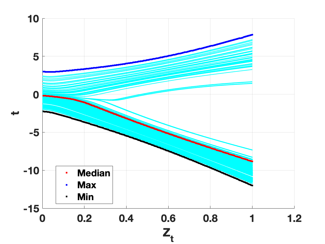
(a) $\rho_{1}=.5N(4,1)+.5N(-10,1)$

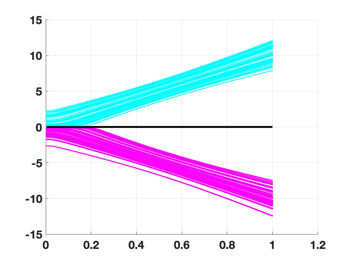
(b) $\rho_{1}=.5N(10,1)+.5N(-10,1)$

Figure 2: (a) shows the flow of the minimum, median and maximum values of a set of points, initially distributed according to a standard Gaussian. (b) shows the flow of points from a standard Gaussian to a symmetric mixture of two Gaussians and the black line represents $y=0$.

Lemma 4.3.

Let $z_{0}\in\mathbb{R}$ and $z_{t},t\in[0,1]$ be a solution to the ODE (3) with a Lipschitz drift function $v(x,t)$ and initial starting point at $z_{0}$. Then $\mathbb{P}(Z_{t}\leq z_{t})$ is a constant depending $z_{0}$ and $v_{t}$ for all $t$, where $Z_{t}$ is the solution of ODE (3).

The proof of the above lemma is deferred to Appendix A.2.2. In Figure 2 (a) we show the trajectories $(t,Z_{t})$ of $n=101$ datapoints generated from source distribution $\rho_{0}=N(0,1)$ and target distribution $\rho_{1}=.5N(4,1)+.5N(-10,1)$. The blue, red, and green lines are the maximum, median, and minimum of the $n$ data points over time. One can see that the image of the same point at time $t$ continues to preserve the quantile for all $t\in[0,1]$. This phenomenon also leads to interesting geometrical phenomena. For example, Figure 2 (b) shows that for transforming a Gaussian to a symmetric two-component mixture of Gaussians $.5N(10,1)+.5N(-10,1)$, all points above (below) the $Z_{t}=0$ line stay above (below). This now paves the way for our next result.

4.1 Gaussian to a mixture of two Gaussians in $\mathbb{R}^{d}$

Theorem 4.4.

Consider $X_{0}\sim\rho_{0}$ and $X_{1}\sim\rho_{1}$, where $\rho_{1}=\pi N(\mu_{1},I_{d})+(1-\pi)N(\mu_{2},I_{d})$ where $\mu_{i}\in\mathbb{R}^{d}$ ($i\in[2]$), and $\rho_{0}=N(0,I_{d})$. One application of rectified flow yields a straight coupling.

Proof Sketch: Our proof uses the fact that one can always rotate the $d$ dimensional space so that in the rotated basis, the means of the two components of the Gaussian mixture are sparse with two non-zero coefficients (one of which is, in fact, equal (WLOG call this coordinate $1$). Denote the entry of coordinate 1 by $c_{1}$. This rotation, in the isoperimetric mixture case, does not affect the covariance or the straightness of the flow. Conveniently, this rotation also lets us decompose the flow to be analyzed coordinate-wise. To this end, for $i\in\{0,1\}$ and $j\in[d]$, we denote by $\tilde{Z}_{i,j}$ the $j^{th}$ component of the solution to the ODE (Equation (3)) at $t=i$ in the rotated space. We show that, in this case, for all the directions $j$ outside the support of the rotated means, we have $\tilde{Z}_{1,j}=\tilde{Z}_{0,j}$. For coordinate 1, we show that there is a translation, i.e., $\tilde{Z}_{1,1}=\tilde{Z}_{0,1}+c_{1}$. For the remaining coordinate where the component-wise rotated means differ, one uses monotonicity of $v_{t}$ along with Lemma 4.2 to show that the coupling is monotonic and hence straight. Furthermore, along the direction of nonzero means in the rotated basis, according to Lemma 4.3, the map induced by the ODE preserves quantiles. The detailed proof is deferred to Appendix Section A.2.4.

Finally, we come to the Gaussian mixture to Gaussian mixture setting.

Proposition 4.5.

Consider $\mu_{01}=(0,a)^{\top},\mu_{02}=(0,-a)^{\top}$ and $\mu_{11}=(a,a)^{\top},\mu_{12}=(a,-a)^{\top}$ for some $a>0$. Let

$$X_{0}\sim 0.5N(\mu_{01},I_{2})+0.5N(\mu_{02},I_{2}),\quad X_{1}\sim 0.5N(\mu_{11},I_{2})+0.5N(\mu_{12},I_{2}).$$

One application of rectified flow gives a straight coupling.

The intuitive explanation is that even in this case, the flows along each coordinate decouples. The $x-$coordinate goes through a translation, whereas the $y-$coordinate’s velocity function is uniformly Lipschitz, leading to a monotonic coupling along $y-$direction. This, along with Lemma 4.2, shows that the flow along the $y-$axis is also monotonic; hence, one rectification gives a straight coupling. The proof is deferred to the Appendix A.2.5.

5 Experiments

In this section, we present numerical experiments for both synthetic and real data. We primarily explore the effect of the number of discretization steps $T$ and the straightness parameter $\gamma_{2,T}(\mathcal{Z})$ on the $W_{2}$ distance between the target distribution and the distribution of the generated sample after 1-rectification. The code is available at https://github.com/bansal-vansh/rectified-flow

(a)

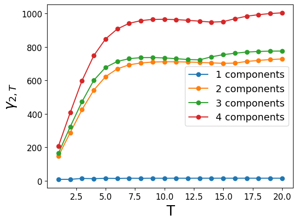
(b)

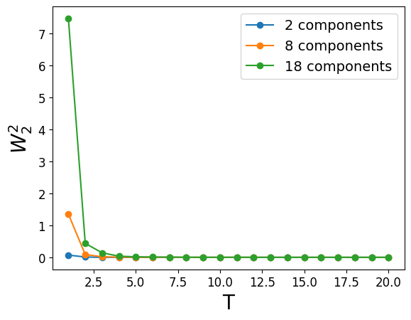
(c)

Figure 3: Plots showing squared Wasserstein distance and $\gamma_{2,T}(\mathcal{Z})$ for the synthetic datasets. (a) shows the $W_{2}^{2}(\widehat{\rho}_{\rm{data}},\rho_{1})$ vs $T$ for mixtures of Gaussians with varying components. (b) shows the straightness parameter $\gamma_{2,T}(\mathcal{Z})$ vs $T$ for the same respective distributions. (c) shows the $W_{2}^{2}(\widehat{\rho}_{\rm{data}},\rho_{1})$ vs $T$ for the Checker-board dataset with varying components. We observe that the straightness of the flow decreases with increasing number of mixture components.

5.1 Synthetic data

For simulated data, we consider the following two examples: 1) Flow from standard Gaussian to a balanced mixture of Gaussian distributions in $\mathbb{R}^{2}$ with varying components, and 2) Flow from standard Gaussian to a checker-board distribution (see Figure 4) with varying components. Next, we discuss our findings in detail below.

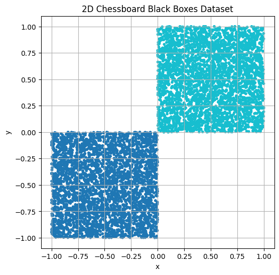
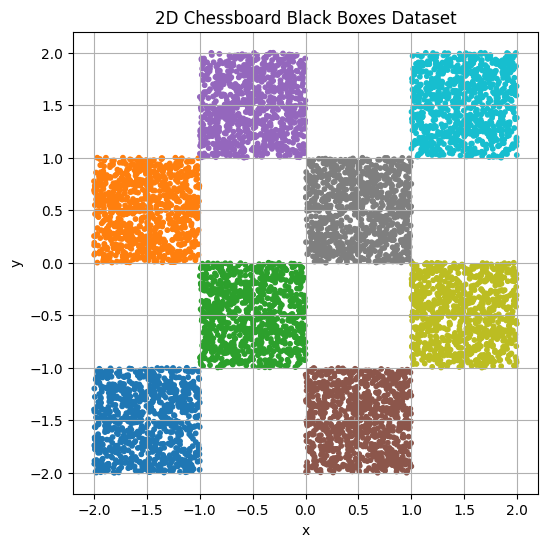
(a)	(b)

Figure 4: (a) Checker-board distribution with 2 components. (b) Checker-board distribution with 8 components.

Example 1: For the mixture of Gaussians example, we vary the number of components $K$ within $\{1,2,3,4\}$ with equal cluster probability and unit variance. For $K=1$ we set mean of the target distribution to be $\mu_{1}=(7/\sqrt{2},5/\sqrt{2})^{\top}$. Similarly, for $K=2$, we set $\mu_{1}=(2,5/\sqrt{2})^{\top},\mu_{2}=(-2,5/\sqrt{2})^{\top}$; for $K=3$ we set $\mu_{1}=(7/\sqrt{2},5/\sqrt{2})^{\top},\mu_{2}=(-9/\sqrt{2},5/\sqrt{2})^{\top},\mu_{3}=(-5/\sqrt{2},-2/\sqrt{2})^{\top}$; and for $K=4$ we set same $\mu_{1},\mu_{2},\mu_{3}$ as in the $K=3$ case with $\mu_{4}=(5/\sqrt{2},-8/\sqrt{2})^{\top}$.

We started with independent coupling in each of the four cases and exploited the analytical form of $v_{t}(x)$ in (A.18) to generate the 1-rectified flow. Therefore, the approximation error ${\varepsilon_{\rm vl}}=0$ in this case. Figure 3(a) shows that $W_{2}(\widehat{\rho}_{\rm{data}},\rho_{1})$ decreases with increasing number of discretization $T$, which is indeed consistent with our main theoretical findings. Moreover, $W_{2}$ distance is consistently larger for the flow corresponding to a larger number of components. This could be explained by the straightness parameter $\gamma_{2,T}(\mathcal{Z})$. Figure 3(b) shows that $\gamma_{2,T}(\mathcal{Z})$ is larger when $K$ is large, which in turn increases the Wasserstein distance.

Example 2: We consider the checker-board distribution with 2,8 and 18 components. We use training datasets of size 10,000 to train a feed-forward neural network in order to learn the velocity drift function and evaluate $W_{2}^{2}(\widehat{\rho}_{\rm{data}},\rho_{1})$ using POT (Feydy et al., 2019) for different levels of discretization $T$ over test data of size 5000. Figure 3(c) also shows that larger component size has a negative effect on the Wasserstein distance, i.e., which stems from the fact that a larger number of components typically pushes the flow away from straightness.

5.2 Real Data

For the real data experiments, we consider the MNIST and FashionMNIST datasets. In both examples, we use the UNet architecture to train our model on the training data, and then evaluate the Wasserstein distance on the test data.

For MNIST data, we construct 3-different datasets. The first one only contains the digits $\{0,1,2\}$, the second one only contains $\{0,1,2,\ldots,6\}$ and the final one contain $\{0,1,2,\ldots,9\}$. Essentially, these datasets contain multiple modes which resembles the nature of the synthetic dataset examples discussed in the previous section. Figure 5(a) shows that the Wasserstein distance is larger when there is more number of components in the dataset. Essentially, more components make the flow more non-straight, and hence convergence in Wasserstein is affected.

We also consider similar datasets for the FashionMNIST example consisting of the first 3 labels, the first 7 labels, and the first 10 labels. Figure 5(b) also shows that the presence of a higher number of components negatively affects the Wasserstein distance, which also indicates the departure of the flow from straightness.

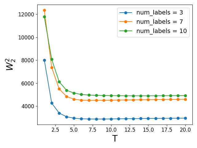
(a)

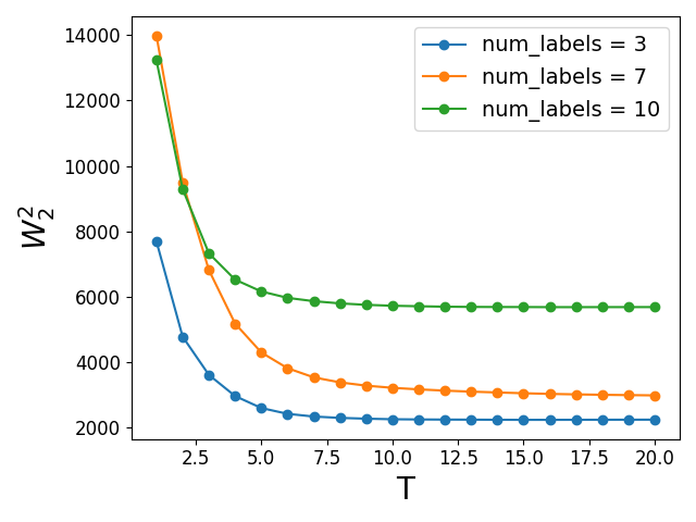
(b)

Figure 5: (a) shows the plot of squared Wasserstein distance $W_{2}^{2}(\widehat{\rho}_{\rm{data}},\rho_{1})$ vs $T$ for the MNIST dataset with a varying numbers of labels, and hence, conditional modes. (b) shows a similar plot for the FashionMNIST dataset

6 Conclusion

Rectified Flow (RF), a newly introduced alternative to diffusion models, is known for its ability to learn straight flow trajectories from noise to data. Straight flows are desirable because they require fewer Euler discretization steps. In this paper, we present the first theoretical analysis of the Wasserstein distance between the sampling distribution of RF and the target distribution. We also formulate a new measure of straightness and show that the error rate is characterized by this measure, the number of discretization steps, and the approximation error for estimating the velocity function. We also use illustrative examples to showcase situations where two rectifications are sufficient to achieve a straight flow. This theoretically validates the empirical findings in several recent works. We present empirical results as a proof of concept for our theoretical results.

Appendix

Appendix A.1 Proofs of Section 3

A.1.1 Proof of Theorem 3.2

Let $\{\rho_{t}\}_{t\in[0,1]}$ and $\{\tilde{\rho}_{t}\}_{t\in[0,1]}$ be distribution of the solution of (3) and (4) respectively. Let $\pi_{t}$ be the optimal coupling between $\rho_{t}$ and $\tilde{\rho}_{t}$. Therefore, using Corollary 5.25 of Santambrogio (2015), we have

$$\frac{1}{2}\frac{dW_{2}^{2}(\rho_{t},\tilde{\rho}_{t})}{dt} =\int\left\langle x-y,v_{t}(x)-\widehat{v}_{t}(y)\right\rangle\;d\pi_{t}(x,y)$$

$$=\int\left\langle x-y,v_{t}(x)-\widehat{v}_{t}(x)\right\rangle\;d\pi_{t}(x,y)+\int\left\langle x-y,\widehat{v}_{t}(x)-\widehat{v}_{t}(y)\right\rangle\;d\pi_{t}(x,y)$$

$$\leq\frac{1}{2}\int\left\|{x-y}\right\|_{2}^{2}\;d\pi_{t}(x,y)+\frac{1}{2}\int\left\|{v_{t}(x)-\widehat{v}_{t}(x)}\right\|_{2}^{2}\;d\pi_{t}(x,y)+\widehat{L}\int\left\|{x-y}\right\|_{2}^{2}\;d\pi_{t}(x,y)$$

$$=(1/2+\widehat{L})W_{2}^{2}(\rho_{t},\tilde{\rho}_{t})+\frac{b(t)}{2}.$$

Solving the above differential inequality leads to the following inequality

$$W_{2}^{2}(\rho_{\tau},\tilde{\rho}_{\tau})\leq W_{2}^{2}(\rho_{0},\tilde{\rho}_{0})+e^{1+2\widehat{L}}\int_{0}^{\tau}b(t)\;dt.$$

The result follows by noting that $W_{2}^{2}(\rho_{0},\tilde{\rho}_{0})=0$ and setting $\tau=1$.

A.1.2 Proof of Lemma 3.4

Recall that $S(\mathcal{Z})=\int_{0}^{1}\mathbb{E}\left\|{Z_{1}-Z_{0}-v_{t}(Z_{t})}\right\|_{2}^{2}\;dt$. Also, note that $Z_{1}-Z_{0}=\int_{0}^{1}v_{u}(Z_{u})\;du$. Therefore, we have

$$S(\mathcal{Z}) =\int_{0}^{1}\mathbb{E}\left\|{\int_{0}^{1}[v_{u}(Z_{u})-v_{t}(Z_{t})]\;du}\right\|_{2}^{2}\;dt$$

$$=\int_{0}^{1}\mathbb{E}\left\|{\int_{0}^{1}\int_{t}^{u}\dot{v}_{\tau}(Z_{\tau})\;d\tau\;du}\right\|_{2}^{2}\;dt$$

$$=\int_{0}^{1}\mathbb{E}\left\|{\int_{0}^{1}\int_{0}^{1}\dot{v}_{\tau}(Z_{\tau})\;d\tau\;du}\right\|_{2}^{2}\;dt$$

$$\leq\int_{0}^{1}\mathbb{E}\left[\int_{0}^{1}\left|{t-u}\right|\int_{t\wedge u}^{t\vee u}\left\|{\dot{v}_{\tau}(Z_{\tau})}\right\|_{2}^{2}\;d\tau\;du\right]\;dt$$

$$\leq\int_{0}^{1}\mathbb{E}\int_{0}^{1}\int_{0}^{1}\left\|{\dot{v}_{\tau}(Z_{\tau})}\right\|_{2}^{2}\;d\tau\;du$$

$$\leq\int_{0}^{1}\mathbb{E}\left\|{\dot{v}_{\tau}(Z_{\tau})}\right\|_{2}^{2}\;d\tau=\gamma_{1}(\mathcal{Z}).$$

Moreover, note that

$$\gamma_{1}(\mathcal{Z})=\sum_{i=1}^{T}(t_{i}-t_{i-1}).\frac{1}{t_{i}-t_{i-1}}\int_{t_{i-1}}^{t_{i}}\mathbb{E}\left\|{\dot{v}_{\tau}(Z_{\tau})}\right\|_{2}^{2}\;d\tau\leq\gamma_{2,T}(\mathcal{Z}).$$ (A.6)

This shows the desired inequality.

For the second part, first note that the $t_{i}-t_{i-1}=1/T$. Therefore,

$$\gamma_{1}(\mathcal{Z})=\frac{1}{T}\sum_{i=1}^{T}\frac{1}{t_{i}-t_{i-1}}\int_{t_{i-1}}^{t_{i}}\mathbb{E}\left\|{\dot{v}_{\tau}(Z_{\tau})}\right\|_{2}^{2}\;d\tau\geq\frac{\gamma_{2,T}(\mathcal{Z})}{T}.$$

The above inequality along with (A.6) tells that $\gamma_{1}(\mathcal{Z})=0$ iff $\gamma_{2,T}(\mathcal{Z})=0$.

Now, due to the inequality $S(\mathcal{Z})\leq\gamma_{1}(\mathcal{Z})$, we have $S(\mathcal{Z})=0$ if $\gamma_{1}(\mathcal{Z})=0$. For the other direction, let us assume $S(\mathcal{Z})=0$. This shows that $v_{t}(Z_{t})=Z_{1}-Z_{0}$ almost surely in $t$ and $(Z_{0},Z_{1})$. This shows that $\dot{v}_{t}(Z_{t})=0$ almost surely. Hence the result follows.

A.1.3 Proof of Theorem 3.5

Recall that for a given partition $0=t_{0}<t_{1}<\ldots<t_{T}=1$ of the interval $[0,1]$ of equidistant points $\{t_{i}\}_{0\leq i\leq T}$ with $h:=T^{-1}$, we follow the Euler discretized version of the of ODE (4) to obtain the sample estimates:

$$\widehat{Y}_{t_{i}}=\widehat{Y}_{t_{i-1}}+h\widehat{v}_{t_{i}}(\widehat{Y}_{t_{i}}),\quad\widehat{Y}_{0}=Z_{0}.$$

Before analyzing the discretization error, we introduce the following interpolation process for $t\in[t_{i},t_{i+1}]$ and each $i\in\{0,\ldots,T\}$:

$${\frac{\rm d}{\rm dt}}\bar{Y}_{t}=\widehat{v}_{t_{i}}(\bar{Y}_{t_{i}}),\quad\bar{Y}_{t_{i}}=\widehat{Y}_{t_{i}}.$$ (A.7)

The above ODE flow gives us a continuous interpolation between $\widehat{Y}_{t_{i}}$ and $\widehat{Y}_{t_{i+1}}$. Coupled with the above flow equation and the ODE flow (5), we have the following almost sure differential inequality for $t\in[t_{i},t_{i+1}]$:

$${\frac{\rm d}{\rm dt}}\|Z_{t}-\bar{Y}_{t}\|_{2}^{2} =2\left\langle Z_{t}-\bar{Y}_{t},{\frac{\rm d}{\rm dt}}Z_{t}-{\frac{\rm d}{\rm dt}}\bar{Y}_{t}\right\rangle$$

$$=2\left\langle Z_{t}-\bar{Y}_{t},v_{t}(Z_{t})-\widehat{v}_{t_{i}}(\bar{Y}_{t_{i}})\right\rangle$$

$$\leq\widehat{L}\|Z_{t}-\bar{Y}_{t}\|_{2}^{2}+\|v_{t}(Z_{t})-\widehat{v}_{t_{i}}(\bar{Y}_{t_{i}})\|_{2}^{2}/\widehat{L}$$

Multiplying $e^{-\widehat{L}(t-t_{i})}$ on both sides of the above inequality and rearranging the terms leads to

$$e^{-\widehat{L}(t-t_{i})}{\frac{\rm d}{\rm dt}}\|Z_{t}-\bar{Y}_{t}\|_{2}^{2}-e^{-\widehat{L}(t-t_{i})}\widehat{L}\|Z_{t}-\bar{Y}_{t}\|_{2}^{2}\leq e^{-\widehat{L}(t-t_{i})}\|v_{t}(Z_{t})-\widehat{v}_{t_{i}}(\bar{Y}_{t_{i}})\|_{2}^{2}/\widehat{L}.$$

$$\Leftrightarrow{\frac{\rm d}{\rm dt}}\{e^{-\widehat{L}(t-t_{i})}\|Z_{t}-\bar{Y}_{t}\|_{2}^{2}\}\leq e^{-\widehat{L}(t-t_{i})}\|v_{t}(Z_{t})-\widehat{v}_{t_{i}}(\bar{Y}_{t_{i}})\|_{2}^{2}/\widehat{L}\leq\|v_{t}(Z_{t})-\widehat{v}_{t_{i}}(\bar{Y}_{t_{i}})\|_{2}^{2}/\widehat{L}.$$

$$\Leftrightarrow\|Z_{t_{i+1}}-\widehat{Y}_{t_{i+1}}\|_{2}^{2}\leq e^{\widehat{L}(t_{i+1}-t_{i})}\|Z_{t_{i}}-\widehat{Y}_{t_{i}}\|_{2}^{2}+\frac{e^{\widehat{L}(t_{i+1}-t_{i})}}{\widehat{L}}\int_{t_{i}}^{t_{i+1}}\|v_{t}(Z_{t})-\widehat{v}_{t_{i}}(\bar{Y}_{t_{i}})\|_{2}^{2}\;dt.$$

Define $\Delta_{i}:=\mathbb{E}\|Z_{t_{i}}-\widehat{Y}_{t_{i}}\|_{2}^{2}$. Using the above inequality we have

$$\Delta_{i+1}$$ (A.8)

$$\leq e^{\widehat{L}h}\Delta_{i}+\frac{e^{\widehat{L}h}}{\widehat{L}}\int_{t_{i}}^{t_{i+1}}\mathbb{E}\|v_{t}(Z_{t})-\widehat{v}_{t_{i}}(\widehat{Y}_{t_{i}})\|_{2}^{2}\;dt$$

$$\leq e^{\widehat{L}h}\Delta_{i}+\frac{3e^{\widehat{L}h}}{\widehat{L}}\left\{\underbrace{\int_{t_{i}}^{t_{i+1}}\mathbb{E}\|v_{t}(Z_{t})-v_{t_{i}}(Z_{t_{i}})\|_{2}^{2}\;dt}_{T_{1}}+\underbrace{\int_{t_{i}}^{t_{i+1}}\mathbb{E}\|v_{t_{i}}(Z_{t_{i}})-\widehat{v}_{t_{i}}(Z_{t_{i}})\|_{2}^{2}\;dt}_{T_{2}}+\underbrace{\int_{t_{i}}^{t_{i+1}}\mathbb{E}\|\widehat{v}_{t_{i}}(Z_{t_{i}})-\widehat{v}_{t_{i}}(\widehat{Y}_{t_{i}})\|_{2}^{2}\;dt}_{T_{3}}\right\}.$$

Now we will bound each of the last three terms on the right-hand side of the above inequality.

Bounding $T_{1}$. For the first term, we have

$$\mathbb{E}\|v_{t}(Z_{t})-v_{t_{i}}(Z_{t_{i}})\|_{2}^{2} =\mathbb{E}\left\|{\int_{t_{i}}^{t}{\frac{\rm d}{\rm d\tau}}v_{\tau}(Z_{\tau})\;d\tau}\right\|_{2}^{2}$$ (A.9)

$$\leq(t-t_{i})\int_{t_{i}}^{t}\mathbb{E}\left\|{{\frac{\rm d}{\rm d\tau}}v_{\tau}(Z_{\tau})}\right\|_{2}^{2}\;d\tau\quad$$

$$\leq h^{2}\gamma_{i},$$

where $\gamma_{i}=\frac{1}{t_{i+1}-t_{i}}\int_{t_{i}}^{t_{i+1}}\mathbb{E}\|{\frac{\rm d}{\rm d\tau}}v_{\tau}(Z_{\tau})\|_{2}^{2}\;d\tau$. This shows that $T_{1}\leq h^{3}\gamma_{i}$.

Bounding $T_{2}$. The term $T_{2}$ is bounded by $h{\varepsilon^{2}_{\rm vl}}$ as $\mathbb{E}\|v_{t_{i}}(Z_{t_{i}})-\widehat{v}_{t_{i}}(Z_{t_{i}})\|_{2}^{2}\leq{\varepsilon^{2}_{\rm vl}}$ (Assumption 3.1(a)).

Bounding $T_{3}$. For the final term we will use that $\widehat{v}_{t_{i}}$ is $\widehat{L}$-Lipschitz. This entails that $T_{3}\leq\widehat{L}h\Delta_{i}$. Plugging these bounds in the recursion formula (A.8), we get

$$\Delta_{i+1}\leq e^{\widehat{L}h}(1+3\widehat{L}h)\Delta_{i}+3e^{\widehat{L}h}(h^{3}\gamma_{i}+h{\varepsilon^{2}_{\rm vl}})/\widehat{L}.$$

Solving the recursion yields

$$\Delta_{T} \leq e^{T\widehat{L}h}(1+3\widehat{L}h)^{T}\Delta_{0}+\frac{3h^{3}}{\widehat{L}}\left\{\sum_{k=1}^{T}e^{k\widehat{L}h}(1+3\widehat{L}h)^{k-1}\gamma_{T-k}\right\}+\frac{3h}{\widehat{L}}\left\{\sum_{k=1}^{T}e^{k\widehat{L}h}(1+3\widehat{L}h)^{k-1}\right\}{\varepsilon^{2}_{\rm vl}}.$$

Recall that $\gamma_{2,T}(\mathcal{Z}):=\max_{k}\gamma_{k}$. Note that $\Delta_{0}=0$ as $Z_{0}=\widehat{Y}_{0}$. Therefore, we have

$$\Delta_{T}\leq\frac{3e^{4\widehat{L}}}{\widehat{L}^{2}}\left(\frac{\gamma_{2,T}(\mathcal{Z})}{T^{2}}+{\varepsilon^{2}_{\rm vl}}\right).$$

Here we used the fact that

$$\sum_{k=1}^{T}e^{k\widehat{L}h}(1+3\widehat{L}h)^{k-1}\leq\frac{e^{4\widehat{L}}-1}{1+3\widehat{L}h-e^{-\widehat{L}h}}\leq\frac{e^{4\widehat{L}}}{3\widehat{L}h}\leq\frac{e^{4\widehat{L}}}{\widehat{L}h}.$$

Therefore, we have

$$W_{2}^{2}(\widehat{\rho}_{\rm{data}},\rho_{1})\leq\Delta_{T}\leq\frac{3e^{4\widehat{L}}}{\widehat{L}^{2}}\left(\frac{\gamma_{2,T}(\mathcal{Z})}{T^{2}}+{\varepsilon^{2}_{\rm vl}}\right).$$

Appendix A.2 Proofs of Section 4

A.2.1 Proof of Theorem 4.1

Let $X_{0}\sim\mathcal{N}(0,I)$ and $X_{1}\sim\mathcal{N}(\mu,\Sigma)$. Let $\Sigma_{t}=t^{2}\Sigma+(1-t)^{2}I$. Then we have that $X_{t}\sim\mathcal{N}(t\mu,\Sigma_{t}),$. Let the density of $X_{t}$ be $\xi_{t}$ and the score $s_{t}(x)=\nabla_{x}\log\xi_{t}(x)=\Sigma_{t}^{-1}(t\mu-x)$. Therefore, by using (A.17), the drift is given by:

$$v(x,t) =\frac{x}{t}+\frac{1-t}{t}\Sigma_{t}^{-1}(t\mu-x)$$

$$=(1-t)\Sigma_{t}^{-1}\mu+\frac{1}{t}\left({I-(1-t)\Sigma_{t}^{-1}}\right)x$$

So the ODE we want to solve is given by:

$$\frac{dZ_{t}}{dt}-\frac{1}{t}\left({I-(1-t)\Sigma_{t}^{-1}}\right)Z_{t}=(1-t)\Sigma_{t}^{-1}\mu$$ (A.10)

Now we look at the structure of $I-(1-t){\bm{\Sigma}}_{t}^{-1}$. Let the eigendecomposition of $\Sigma=U\Lambda U^{T}$. We will assume $\Sigma$ is full rank. So,

$$I-(1-t)\Sigma_{t}^{-1}=U\Lambda_{t}U^{T}$$

where $\Lambda_{t}=\frac{1}{t}\{I-(1-t)(t^{2}\Lambda+(1-t)^{2}I)^{-1}\}$. This can also be written as:

$$\lambda_{t,i}=\frac{1}{t}\{1-\frac{1-t}{t^{2}\lambda_{i}+(1-t)^{2}}\}=\frac{t(1+\lambda_{i})-1}{t^{2}\lambda_{i}+(1-t)^{2}}$$

Substituting this into Eq A.10, we have:

So, we first get the integrating factors of each eigenvalue.

$$I_{i}(t)=\frac{1}{\sqrt{(1+\lambda_{i})t^{2}-2t+1}}$$

So we have:

$$U\Lambda^{\prime}_{t}U^{T}Z_{t}=U\Lambda^{\prime\prime}_{t}U^{T}\mu+constant$$

where $\lambda^{\prime}_{t,i}=\frac{1}{\sqrt{(1+\lambda_{i})t^{2}-2t+1}}$ and $\lambda^{\prime\prime}_{t,i}=\frac{t}{\sqrt{(1+\lambda_{i})t^{2}-2t+1}}$

This yields,

$$\Sigma^{-1/2}Z_{1}-Z_{0} =\Sigma^{-1/2}\mu$$

$$Z_{1} =\Sigma^{1/2}Z_{0}+\mu$$ (A.11)

A.2.2 Proof of Lemma 4.3

We recall the ODE $\dot{Z}_{t}=v_{t}(Z_{t})$ with $Z_{0}=z_{0}$. As $x\mapsto v_{t}(x)$ is uniformly Lipschitz, there exists a unique solution $\{Z_{t}\}_{t\in[0,1]}$ such that $Z_{0}=z_{0}$. Moreover, the map $H_{t}:z_{0}\mapsto z_{t}$ is monotonically increasing. To see this, let us assume $z_{0}>\tilde{z}_{0}$, but $z_{t}<\tilde{z}_{t}$. Note that $G(\tau):=H_{\tau}(z_{0})-H_{\tau}(\tilde{z}_{0})$ is continuous in $\tau$. Also, $G(0)>0$ and $G(t)<0$. By the intermediate value property, there exists a $t_{0}\in[0,1]$ such that $G(t_{0})=0$, i.e., $z_{t_{0}}=\tilde{z}_{t_{0}}=:z_{0}$. This violates the uniqueness condition of the ODE solution. Hence, $H_{t}$ is monotonically increasing. By monotonicity, it follow that

$${\mathbb{P}}(Z_{t}\leq z_{t})={\mathbb{P}}(H_{t}(Z_{0})\leq H_{t}(z_{0}))={\mathbb{P}}(Z_{0}\leq z_{0}).$$

This finishes the proof.

A.2.3 Gaussian to a mixture of two Gaussians in $\mathbb{R}^{2}$

Proposition A.1.

Consider $\tilde{X}_{0}\sim\mathcal{N}(0,I_{2})$ and $\tilde{X}_{1}\sim\pi\mathcal{N}(\tilde{\mu}_{1},\Lambda)+(1-\pi)\mathcal{N}(\tilde{\mu}_{2},\Lambda)$ where $\Lambda$ is a PSD diagonal matrix in $\mathbb{R}^{2}$. Then, $(\tilde{Z}_{0},\tilde{Z}_{1})=\texttt{Rectify}\left({\tilde{X}_{0},\tilde{X}_{1}}\right)$ is a straight coupling.

Proof.

Let $P$ be the ortho-normal matrix given by $P=\begin{bmatrix}\frac{\tilde{\mu}_{2}-\tilde{\mu}_{1}}{\left\|{\tilde{\mu}_{2}-\tilde{\mu}_{1}}\right\|}&\frac{R(\tilde{\mu}_{2}-\tilde{\mu}_{1})}{\left\|{\tilde{\mu}_{2}-\tilde{\mu}_{1}}\right\|}\end{bmatrix},$ where $R=\begin{bmatrix}0&-1\\ 1&0\end{bmatrix}$ is the skew-symmetric matrix for a 90-degree rotation. We rotate our space using the linear transformation $P$ and obtain the random variables $X_{0}=P\tilde{X}_{0}\sim\mathcal{N}(0,I)$ and $X_{1}=P\tilde{X}_{1}\sim\pi\mathcal{N}(\mu_{1},\Sigma)+(1-\pi)\mathcal{N}(\mu_{2},\Sigma)$, where $\mu_{i}=\begin{bmatrix}x_{i}&y_{i}\end{bmatrix}^{\top}=P\tilde{\mu}_{i}$, $\Sigma=P\tilde{\Lambda}P^{\top}=\Lambda$. Also note that by the above construction of the transformation $P$, $x_{1}=x_{2}:=x.$ We first show that $(Z_{0},Z_{1})=\text{Rectify}(X_{0},X_{1})$ is straight and then argue that an invertible transformation does not hamper straightness.
Let $\Lambda_{t}=t^{2}\Lambda+(1-t)^{2}I$, then, $X_{t}\sim\rho_{t}=\pi\mathcal{N}(t\mu_{1},\Lambda_{t})+(1-\pi)\mathcal{N}(t\mu_{2},\Lambda_{t})$ and the score of $\rho_{t}$, denoted by $s_{t}$ is:

$$s_{t}(z_{t})=\sum_{i=1}^{2}w_{t,i}(z_{t})\Lambda_{t}^{-1}\left({t\mu_{i}-z_{t}}\right)$$

where the quantity $w_{t,1}(z_{t}):=\frac{1}{1+\exp(g_{t}(z_{t}))}$, $w_{t,2}(z_{t})=1-w_{t,1}(z_{t})$, and

$$g_{t}(z) =\log\frac{1-\pi}{\pi}-\frac{1}{2}\left({(z-t\mu_{2})^{T}\Lambda_{t}^{-1}(z-t\mu_{2})-(z_{t}-t\mu_{1})^{T}\Lambda_{t}^{-1}(z-t\mu_{1})}\right)$$

$$=\log\frac{1-\pi}{\pi}-\frac{1}{2}\left({t(\mu_{1}-\mu_{2})^{T}\Lambda_{t}^{-1}z+t^{2}(\mu_{2}^{T}\Lambda_{t}^{-1}\mu_{2}-\mu_{1}^{T}\Lambda_{t}^{-1}\mu_{1})}\right)$$

$$=\log\frac{1-\pi}{\pi}-\frac{1}{2}\left({\frac{t(y_{1}-y_{2})}{t^{2}\lambda_{2}+(1-t)^{2}}z+t^{2}(\mu_{2}^{T}\Lambda_{t}^{-1}\mu_{2}-\mu_{1}^{T}\Lambda_{t}^{-1}\mu_{1})}\right)$$ (A.12)

Then, using (A.17), the drift is given by

$$v_{t}(z_{t}) =\frac{z_{t}}{t}+\frac{1-t}{t}s_{t}(z_{t})$$ (A.13)

$$=\frac{(I-(1-t)\Lambda_{t}^{-1})}{t}z_{t}+(1-t)\Lambda_{t}^{-1}\sum_{i=1}^{2}w_{i,t}(z_{t})\mu_{i}$$ (A.14)

$$=\frac{1}{t}\tilde{\Lambda}_{t}z_{t}+(1-t)\Lambda_{t}^{-1}\begin{pmatrix}x\\ \sum_{i=1}^{2}w_{i,t}(z_{t})y_{i}\end{pmatrix}$$ (A.15)

where we define $\tilde{\Lambda}_{t}:=I-(1-t)\Lambda_{t}^{-1}=I-(1-t)(t^{2}\Lambda+(1-t)^{2}I)^{-1}$.

Now we look at the structure of $\tilde{\Lambda}_{t}$. We will assume $\Lambda=\text{diag}(\lambda_{i})$ is full rank, and $\Lambda_{t}=\text{diag}(t^{2}\lambda_{i}+(1-t)^{2})$.

The diagonal elements of $\tilde{\Lambda}_{t}$

$$\tilde{\lambda}_{t,i}=\frac{1}{t}\left({1-\frac{1-t}{t^{2}\lambda_{i}+(1-t)^{2}}}\right)=\frac{t(1+\lambda_{i})-1}{t^{2}\lambda_{i}+(1-t)^{2}}$$

For now, we have:

$$\frac{dZ_{t,1}}{dt}=\frac{t(1+\lambda_{1})-1}{t^{2}\lambda_{1}+(1-t)^{2}}Z_{t,1}+\frac{1-t}{t^{2}\lambda_{1}+(1-t)^{2}}x$$

Define the integrating factor $I(t)=\exp\left({-\int_{0}^{t}\frac{(1+\lambda_{1})u-1}{(1+\lambda_{1})u^{2}-2u+1}}\right)\;du=\frac{1}{\sqrt{(1+\lambda_{1})t^{2}-2t+1}}$.

Multiplying $I(t)$ in both sides of the above ODE and integrating in $t\in[0,1]$ we get the following almost sure inequality:

$$\frac{Z_{1,1}}{\sqrt{\lambda_{1}}}-Z_{0,1}=x\int_{0}^{1}\frac{1-t}{((1+\lambda_{1})t^{2}-2t+1)^{3/2}}\;dt=x\left[\frac{t}{\sqrt{(1+\lambda_{1})t^{2}-2t+1}}\right]_{0}^{1}=\frac{1}{\sqrt{\lambda_{1}}}x.$$

For the second coordinate, we have:

$$f(Z_{t,2}):=\frac{dZ_{t,2}}{dt}=\frac{t(1+\lambda_{2})-1}{t^{2}\lambda_{2}+(1-t)^{2}}Z_{t,2}+\frac{1-t}{t^{2}\lambda_{2}+(1-t)^{2}}\sum_{i=1}^{2}w_{i,t}(Z_{t,2})y_{i}$$ (A.16)

We check that $|d/d_{x}f(x)|$ is bounded. Using the definition of $g_{t}$ in Eq A.12

$$\left|\frac{d}{dz}f(z)\right| \leq\left|\frac{t(1+\lambda_{2})-1}{t^{2}\lambda_{2}+(1-t)^{2}}\right|+|y_{1}-y_{2}|\left|\frac{1-t}{t^{2}\lambda_{2}+(1-t)^{2}}\frac{d}{dz}(g_{t}(z))\right|$$

$$\leq(1+\lambda_{2})+\frac{(1+\lambda_{2})^{2}|y_{1}-y_{2}|^{2}}{\lambda_{2}^{2}}$$

Therefore, $z\mapsto f(z)$ is uniformly Lipschitz, and henceforth, by Lemma A.2 the map $\psi:Z_{0,2}\mapsto Z_{1,2}$ is monotonically increasing.

The above discussion entails that 1-rectified flow essentially sends $Z_{0}$ through a map $\mathcal{T}:\mathbb{R}^{2}\to\mathbb{R}^{2}$ such that

$$Z_{1}=\mathcal{T}(Z_{0})=\begin{pmatrix}\sqrt{\lambda_{1}}Z_{0,1}+x\\ \psi(Z_{0,2})\end{pmatrix}$$

where $\psi$ is only defined through the ODE (A.16). Therefore, for any $t\in[0,1]$ we have the function

$$h_{t}(w):=(1-t)w+t\mathcal{T}(w)=\begin{pmatrix}(1-t)w_{1}+t(\sqrt{\lambda_{1}}w_{1}+x)\\ (1-t)w_{2}+t\psi(w_{2})\end{pmatrix}$$

to be an invertible function, which essentially leads to the following relationship between the two $\sigma$-fields of interest:

$$\mathscr{F}(h_{t}(Z_{0}))=\mathscr{F}(Z_{0})\quad\text{($\mathscr{F}(X)$ denotes the sigma-field generated by $X$)}$$

for all $t\in[0,1]$. Hence, we finally have

$$\mathbb{E}[\mathcal{T}(Z_{0})-Z_{0}\mid h_{t}(Z_{0})]=\mathbb{E}[\mathcal{T}(Z_{0})-Z_{0}\mid Z_{0}]=\mathcal{T}(Z_{0})-Z_{0}.$$

Now, since $P$ is invertible,

$$v_{t}(\tilde{Z}_{t}) =\mathbb{E}\left[{{\tilde{X}_{1}-\tilde{X}_{0}\mid t\tilde{X}_{1}+(1-t)\tilde{X}_{0}=\tilde{Z}_{t}}}\right]$$

$$=P^{-1}\mathbb{E}\left[{{P\tilde{X}_{1}-P\tilde{X}_{0}\mid t\tilde{X}_{1}+(1-t)\tilde{X}_{0}=\tilde{Z}_{t}}}\right]$$

$$=P^{-1}\mathbb{E}\left[{{P\tilde{X}_{1}-P\tilde{X}_{0}\mid tP\tilde{X}_{1}+(1-t)P\tilde{X}_{0}=P\tilde{Z}_{t}}}\right]$$

$$=P^{-1}\mathbb{E}\left[{{X_{1}-X_{0}\mid tX_{1}+(1-t)X_{0}=Z_{t}}}\right]\quad\quad\text{$\because\,(Z_{0},Z_{1})$ is straight}$$

$$=P^{-1}\left({X_{1}-X_{0}}\right)$$

$$=\tilde{X}_{1}-\tilde{X}_{0}$$

Hence, $(\tilde{Z}_{0},\tilde{Z}_{1})$ is also straight. This finishes the proof.

∎

Lemma A.2.

Consider an ODE of the form

$$\frac{dx_{t}}{dt}=c_{t}\,f_{t}\left({x_{t}}\right)$$

for $t\in[0,1]$ where $x_{t}\in\mathbb{R}$ and $c_{t}>0\text{ for all }t\in(0,1]$.

1. If $\frac{\partial f_{t}(x)}{\partial x}>0,$ i.e., $f_{t}(x)$ is an increasing function of $x$, then $x_{1}$ is a monotonically increasing function of the initial condition $x_{0}$.

2. If $f_{t}(x)$ is a uniformly Lipschitz function for all $t\in[0,1]$, then $x_{1}$ is a monotonically increasing function of the initial condition $x_{0}$.

Proof.

Part (a): Let $x_{t}^{1}$ and $x_{t}^{2}$ be two solutions to the ODE:

$$\frac{dx_{t}}{dt}=c_{t}f_{t}(x_{t}),\quad t\in[0,1],$$

corresponding to the initial conditions $x_{0}^{1}$ and $x_{0}^{2}$, respectively, with $x_{0}^{1}<x_{0}^{2}$. We want to show that $x_{1}^{1}<x_{1}^{2}$.

Define the difference between the two solutions:

$$\Delta x_{t}=x_{t}^{2}-x_{t}^{1}.$$

Taking the derivative, we get:

$$\frac{d}{dt}\Delta x_{t}=\frac{d}{dt}(x_{t}^{2}-x_{t}^{1})=c_{t}\left(f_{t}(x_{t}^{2})-f_{t}(x_{t}^{1})\right).$$

Since $\frac{\partial f_{t}(x)}{\partial x}>0$, we have $f_{t}(x_{t}^{2})>f_{t}(x_{t}^{1})$ for $x_{t}^{2}>x_{t}^{1}$, which implies:

$$\frac{d}{dt}\Delta x_{t}>0,\text{ whenever }\Delta x_{t}>0.$$

Define $t^{*}:=\inf\left\{{t\in(0,1]:\Delta x_{t}\leq 0}\right\}$. Due to inverse map theorem we have $\Delta x_{t^{*}}\leq 0$, and $t^{*}>0$ as $\Delta x_{0}>0$. Also, note that

$$\int_{0}^{t_{1}}\frac{d}{dt}\Delta x_{t}\;dt=\Delta x_{t^{*}}-\Delta x_{0}<0.$$

The above inequality entails that there exists $\tau\in(0,t^{*})$ such that $\frac{d}{dt}\Delta x_{t}<0$, which implies that

$$f_{\tau}(x_{\tau}^{2}) <f_{\tau}(x_{\tau}^{1})$$

$$\implies x_{\tau}^{2} <x_{\tau}^{1}$$

$$\implies\Delta x_{\tau} <0$$

This is again a contradiction to the definition of $t^{*}$ as $\tau<t^{*}$. Therefore, we have $\Delta x_{t}>0$ for all $t\in[0,1]$. In particular we have $x_{1}^{2}>x_{1}^{1}$.

Part (b): If $f_{t}(x)$ is uniformly Lipschitz, then by Picard-Lindelof theorem, for any tuple $(t_{0},x_{0})$, there exists only solution $\{x_{t}\}_{t\in[0,1]}$ passing through $x_{0}$ at time $t_{0}$.

Now, following the notation in part (a), let $x_{t}^{1}\leq x_{t}^{2}$ for some $t$. As $H_{t}:x_{0}\mapsto x_{t}$ is continuous, so is $G(\tau):=H_{\tau}(x_{0}^{2})-H_{\tau}(x_{0}^{1})$. However, $G(0)>0$ and $G(t)\leq 0$. By intermediate value property, there exists $t_{0}\in(0,t]$, such that $G(t_{0})=0\Rightarrow x_{t_{0}}^{2}=x_{t_{0}}^{1}$. This contradicts the uniqueness property of the ODE solution. therefore, we have $x_{t}^{2}>x_{t}^{1}$ for all $t$. Then the result follows by setting $t=1$ ∎

A.2.4 Proof of Theorem 4.4

Proof.

Let $\tilde{X}_{0},\tilde{X}_{1}\in\mathbb{R}^{d}$ for $d\geq 2$, where $\tilde{X}_{0}\sim\mathcal{N}(0,I)$ and $\tilde{X}_{1}\sim\sum_{i=1}^{2}\pi_{i}\,\mathcal{N}(\tilde{\mu}_{i},\sigma^{2}I)$ with $\sigma^{2}=1$ (for simplicity). We start with the matrix $\tilde{M}=\begin{bmatrix}\tilde{\mu}_{1}&\tilde{\mu}_{2}\end{bmatrix}$ and perform a QR decomposition: $\tilde{M}=\tilde{Q}\tilde{R}$, where $\tilde{Q}\in\mathbb{R}^{d\times 2}$ is an orthonormal matrix that spans the subspace of $\tilde{\mu}_{1}$ and $\tilde{\mu}_{2}$.

Next, we extend $\tilde{Q}$ to a complete orthonormal basis for $\mathbb{R}^{d}$ using $\tilde{Q}^{\prime}\in\mathbb{R}^{d\times(d-2)}$, which spans the orthogonal complement of the column space of $\tilde{Q}$. We define $Q=\begin{bmatrix}\tilde{Q}&\tilde{Q}^{\prime}\end{bmatrix}^{\top}$. This projection guarantees that:

$$Q\tilde{\mu}_{1}=(x_{1},y_{1},0,\ldots,0)^{\top},\quad Q\tilde{\mu}_{2}=(x_{2},y_{2},0,\ldots,0)^{\top}$$

i.e., only the first two components are non-zero.

To equalize one of the components, we apply a rotation matrix $R(\theta)\in\mathbb{R}^{d\times d}$, which rotates the first two components while leaving the others unchanged:

$$R(\theta)=\begin{bmatrix}\cos\theta&-\sin\theta&0\\ \sin\theta&\cos\theta&0\\ 0&0&I_{d-2}\end{bmatrix}$$

We set $\theta$ as:

$$\theta=\tan^{-1}\left(\frac{y_{2}-y_{1}}{x_{1}-x_{2}}\right)$$

This ensures that the second components of $R(\theta)Q\tilde{\mu}_{1}$ and $R(\theta)Q\tilde{\mu}_{2}$ are identical.

Finally, we define the overall transformation as $P=R(\theta)Q$. This matrix $P\in\mathbb{R}^{d\times d}$ is orthonormal (and hence, invertible) since it is the product of two orthonormal matrices. The transformation $P$, not only makes the last $d-1$ coordinates of the means identical but also reduces the effective dimension of the flow to two.

Now, we rotate our space using the linear transformation $P$ and obtain the distributions $X_{0}=P\tilde{X}_{0}\sim\mathcal{N}(0,I)$ and $X_{1}=P\tilde{X}_{1}\sim\sum_{i=1}^{2}\pi_{i}\,\mathcal{N}(\mu_{i},\Sigma)$, where $\mu_{i}=P\tilde{\mu}_{i}$, $\Sigma=P\tilde{\Sigma}P^{\top}=I$. Also note that by the above construction of the transformation $P$, $\mu_{1,k}=\mu_{2,k}:=c_{k}.$ for all $k\in[d]\backslash\left\{{1}\right\}$. We first show that $(Z_{0},Z_{1})=\text{Rectify}(X_{0},X_{1})$ is straight and then argue that an invertible transformation does not hamper straightness.
To proceed, we apply the Rectify procedure on $(X_{0},X_{1})$ and obtain the following ODE:

$$v_{t}(Z_{t})=\frac{dZ_{t}}{dt} =\frac{(2t-1)Z_{t}}{\sigma_{t}^{2}}+\frac{1-t}{\sigma_{t}^{2}}\sum_{i=1}^{2}w_{i}(Z_{t})\mu_{i}$$

For $k\in[d]\backslash\left\{{1}\right\}$, we have that

$$\frac{dZ_{t,k}}{dt} =\frac{(2t-1)Z_{t,k}}{\sigma_{t}^{2}}+c_{k}$$

Hence, using (A.11) the final mapping is just a translation given by $Z_{1,k}=Z_{0,k}+c_{k}$. However, for the first co-ordinate, for $g_{t}(Z_{t,1})=\log\left({\frac{\pi_{2}}{\pi_{1}}}\right)-\frac{1}{2\sigma_{t}^{2}}\left({\left({Z_{t,1}-t\mu_{2,1}}\right)^{2}-\left({Z_{t,1}-t\mu_{1,1}}\right)^{2}}\right)$, we have

$$\frac{dZ_{t,1}}{dt} =\frac{(2t-1)Z_{t,1}}{\sigma_{t}^{2}}+\frac{1-t}{\sigma_{t}^{2}}\left({\frac{\mu_{1,1}+\mu_{2,1}\exp\left({g_{t}(Z_{t,1})}\right)}{1+\exp\left({g_{t}(Z_{t,1})}\right)}}\right)$$

The reasoning used to demonstrate straightness from this point forward is identical to that of Proposition A.1. ∎

A.2.5 Proof of Proposition 4.5

Proof.

Consider ${\bm{\mu}}_{01}=(0,a)^{\top},{\bm{\mu}}_{02}=(0,-a)^{\top}$ and ${\bm{\mu}}_{11}=(a,a)^{\top},{\bm{\mu}}_{12}=(a,-a)^{\top}$ for some $a>0$. Let

$$X_{0}\sim 0.5\mathcal{N}({\bm{\mu}}_{01},I)+0.5\mathcal{N}({\bm{\mu}}_{02},I),\quad X_{1}\sim 0.5\mathcal{N}({\bm{\mu}}_{11},I)+0.5\mathcal{N}({\bm{\mu}}_{12},I).$$

In this case, the velocity functions in $x$ and $y$-direction for 1-rectification turns out to be

$$u_{t}(x)=\frac{\left(2t-1\right)x}{\sigma_{t}^{2}}+\frac{(1-t)a}{\sigma_{t}^{2}},$$

$$v_{t}(y)=\frac{\left(2t-1\right)y}{\sigma_{t}^{2}}$$

$$+\frac{a}{\sigma_{t}^{2}}\cdot\frac{\exp\left(-\frac{\left(y-a\right)^{2}}{2\sigma_{t}^{2}}\right)\left(1-2t\right)-\ \exp\left(-\ \frac{\left(y+a\right)^{2}}{2\sigma_{t}^{2}}\right)\left(1-2t\right)+\exp\left(-\frac{\left(y\ -\ \left(2t-1\right)a\right)^{2}}{2\sigma_{t}^{2}}\right)-\exp\left(-\frac{\left(y\ +\ \left(2t-1\right)a\right)^{2}}{2\sigma_{t}^{2}}\right)}{\exp\left(-\frac{\left(y-a\right)^{2}}{2\sigma_{t}^{2}}\right)+\ \exp\left(-\ \frac{\left(y+a\right)^{2}}{2\sigma_{t}^{2}}\right)+\exp\left(-\frac{\left(y\ -\ \left(2t-1\right)a\right)^{2}}{2\sigma_{t}^{2}}\right)+\exp\left(-\frac{\left(y\ +\ \left(2t-1\right)a\right)^{2}}{2\sigma_{t}^{2}}\right)}.$$

Next, we will take the derivative of $v_{t}(y)$ with respect to $y$. For notational brevity, let us define

$$e_{1}(y)=\exp\left(-\frac{\left(y-a\right)^{2}}{2\sigma_{t}^{2}}\right)(1-2t),$$

$$e_{2}(y)=\exp\left(-\frac{\left(y+a\right)^{2}}{2\sigma_{t}^{2}}\right)(1-2t),$$

$$e_{3}(y)=\exp\left(-\frac{\left(y-a(2t-1)\right)^{2}}{2\sigma_{t}^{2}}\right),$$

$$e_{4}(y)=\exp\left(-\frac{\left(y+a(2t-1)\right)^{2}}{2\sigma_{t}^{2}}\right).$$

Then we have

$$\left|{\frac{dv_{t}(y)}{dy}}\right|\leq\frac{2t-1}{\sigma_{t}^{2}}+\frac{a^{2}}{\sigma_{t}^{4}}\cdot\frac{4\{e_{1}(y)e_{2}(y)+e_{2}(y)e_{3}(y)+e_{3}(y)e_{4}(y)+e_{4}(y)e_{1}(y)\}}{(\sum_{j=1}^{4}e_{j}(y))^{2}}\leq 2+4a^{2}.$$

We used the basic inequalities $4(ab+bc+cd+da)\leq(a+b+c+d)^{2}$ and $\sigma_{t}^{2}\geq 1/2$ in the last step of the above display.

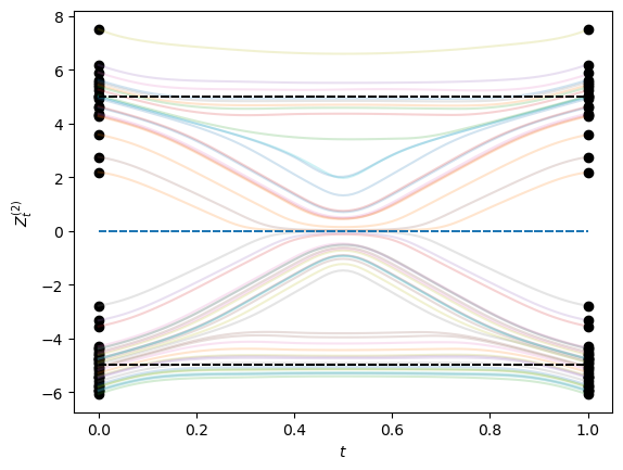
Figure A.1: 1-rectified flow in $y$-direction for GMM

This shows that $v_{t}(y)$ is uniformly Lipschitz. This entails that the map $\mathcal{T}:\mathbb{R}\to\mathbb{R}$ that sends $y_{0}$ to a point $y_{1}\in\mathbb{R}$, and defined through the ODE

$${\frac{\rm d}{\rm dt}}Y_{t}=v_{t}(Y_{t});\;Y_{0}=y_{0},$$

is an injective map due to the uniqueness of the solution of the above ODE. Also, we denote by $Y_{t}^{y_{0}}$ the solution of the above ODE.

To show the strict increasing property of $\mathcal{T}$, let us consider the same ODE with $Y_{0}=\tilde{y}_{0}<y_{0}$. We also consider the solution $Y_{t}^{\tilde{y}_{0}}$. Consider the function $L_{t}:=Y_{t}^{y_{0}}-Y_{t}^{\tilde{y}_{0}}$, which is also continuous in $t\in[0,1]$. To prove increasing property, it is enough to show that $L_{1}>0$. Let us assume that $L_{1}\leq 0$. We already know $L_{0}>0$, and hence by Intermediate Value Property, we have there exists a $\tau\in(0,1]$ such that $L_{\tau}=0$. This entails that there exists $y_{\tau}\in\mathbb{R}$ such that $Y_{\tau}^{y_{0}}=Y_{\tau}^{\tilde{y_{0}}}=y_{\tau}$. This shows that we have two different solutions of the ODE passing through $(\tau,y_{\tau})$, which is a contradiction. This proves the coveted strict increasing property of $\mathcal{T}$. Hence, we have a straight coupling by similar argument as in previous section. ∎

Appendix A.3 Auxiliary results

A.3.1 Connection between score and drift

Let $X_{0}=Z\sim\mathcal{N}(0,I)$ and $X_{1}=X\sim\rho_{\rm{data}}$. Let the density of $X_{t}=tX+(1-t)Z$ be $\xi_{t}$. Then Tweedie’s formula (Robbins (1992)) gives that $\mathbb{E}\left[{{tX\mid X_{t}=x}}\right]=x+(1-t)^{2}s_{t}(x)$ where $s_{t}(x)=\nabla\log\xi_{t}(x)$

We have that

$$v_{t}(x) =\mathbb{E}[X-Z\mid X_{t}=x]$$

$$=\mathbb{E}[\frac{X-X_{t}}{1-t}\mid X_{t}=x]$$

$$=\frac{x+(1-t)^{2}s_{t}(x)}{t(1-t)}-\frac{x}{(1-t)}\quad(\text{applying Tweedie's formula})$$

$$=\frac{x}{t}+\left({\frac{1-t}{t}}\right)s_{t}(x)$$ (A.17)

A.3.2 Auxiliary results for Gaussian mixture to Gaussian mixture flow

In this section, we will procure a formula of the drift function for 1-rectified flow from a Gaussian mixture to another Gaussian mixture. Let $X_{0}\sim\frac{1}{K_{0}}\sum_{i=1}^{K_{0}}\mathcal{N}(\mu_{0i},\sigma^{2}I)$, $X_{1}\sim\frac{1}{K_{1}}\sum_{i=1}^{K_{1}}\mathcal{N}(\mu_{1i},\sigma^{2}I)$, and $X_{t}=tX_{1}+(1-t)X_{0}$.

$$v_{t}(x) =\mathbb{E}\left[{{X_{1}-X_{0}\mid X_{t}=x}}\right]$$

$$=\mathbb{E}\left[{{\frac{X_{1}-X_{t}}{1-t}\mid X_{t}=x}}\right]$$

$$=\frac{1}{t(1-t)}\left({\mathbb{E}\left[{{tX_{1}\mid X_{t}=x}}\right]-tx}\right)$$

$$=\frac{1}{t(1-t)}\left({\frac{1}{K_{0}}\sum_{i=1}^{K_{0}}\frac{p_{t}^{(i)}(x)}{p_{t}(x)}\mathbb{E}\left[{{tX_{1}\mid X_{t}^{(i)}=x}}\right]-tx}\right)$$

$$=\frac{1}{t(1-t)}\left({\frac{1}{K_{0}}\sum_{i=1}^{K_{0}}\frac{p_{t}^{(i)}(x)}{p_{t}(x)}\left({x-(1-t)\mu_{0i}+\tilde{\sigma}_{t}^{2}s_{t}^{(i)}(x)}\right)-tx}\right),\quad\hfill\text{where }\tilde{\sigma}_{t}^{2}=(1-t)^{2}\sigma^{2}$$

$$=\frac{x}{t}+\frac{(1-t)\sigma^{2}}{t}\left({\frac{1}{K_{0}}\sum_{i=1}^{K_{0}}\frac{p_{t}^{(i)}(x)}{p_{t}(x)}\left({s_{t}^{(i)}(x)-\frac{\mu_{0i}}{1-t}}\right)}\right)$$

where $p_{t}^{(i)}(x)=\text{Law}(tX_{1}+(1-t)\mathcal{N}(\mu_{0i},\sigma^{2}))=\frac{1}{K_{1}}\sum_{j=1}^{K_{1}}\mathcal{N}(\underbrace{t\mu_{1j}+(1-t)\mu_{0i}}_{\mu_{tj}^{(i)}},\sigma_{t}^{2})$, $\sigma_{t}^{2}=(t^{2}+(1-t)^{2})\sigma^{2}$.

$$s_{t}^{(i)}(x)=\nabla_{x}\log p_{t}^{(i)}(x)=\frac{1}{\sigma^{2}_{t}}\left({\sum_{j=1}^{K_{1}}w_{j}^{(i)}(x)\mu^{(i)}_{tj}-x}\right),$$

where

$$w_{j}^{(i)}(x)=\frac{\exp\left({\frac{-\left\|{x-\mu^{(i)}_{tj}}\right\|^{2}}{2\sigma_{t}^{2}}}\right)}{\sum_{j}\exp\left({\frac{-\left\|{x-\mu^{(i)}_{tj}}\right\|^{2}}{2\sigma_{t}^{2}}}\right)}$$

A.3.3 Gaussian to a Mixture of Gaussian case

Let $X_{0}\sim\mathcal{N}\left({0,I}\right)$ and $X_{1}\sim\sum_{i}\pi_{i}\mathcal{N}\left({\mu_{i},\sigma^{2}_{i}I}\right)$. Let $X_{t}=tX_{1}+(1-t)X_{0}$, then using (A.17), we have

$$v_{t}(x)=\frac{x}{t}+\frac{1-t}{t}s_{t}(x)$$ (A.18)

where, $s_{t}(x)=\nabla_{x}\log p_{t}(x)$ is given by

$$s_{t}(x)=\sum_{i}w_{i,t}(x)\left({\frac{t\mu_{i}-x}{\sigma^{2}_{i,t}}}\right),$$

$\sigma^{2}_{i,t}=(1-t)^{2}+t^{2}\sigma^{2}_{i}$ and

$$w_{i,t}(x)=\frac{\pi_{i}\exp\left({\frac{-\left\|{x-t\mu_{i}}\right\|^{2}}{2\sigma_{i,t}^{2}}}\right)}{\sum_{j}\pi_{j}\exp\left({\frac{-\left\|{x-t\mu_{j}}\right\|^{2}}{2\sigma_{i,t}^{2}}}\right)}$$

References

- Albergo & Vanden-Eijnden (2022) Michael S Albergo and Eric Vanden-Eijnden. Building normalizing flows with stochastic interpolants. arXiv preprint arXiv:2209.15571, 2022.
- Albergo et al. (2023) Michael S Albergo, Nicholas M Boffi, and Eric Vanden-Eijnden. Stochastic interpolants: A unifying framework for flows and diffusions. arXiv preprint arXiv:2303.08797, 2023.
- Balaji et al. (2022) Yogesh Balaji, Seungjun Nah, Xun Huang, Arash Vahdat, Jiaming Song, Qinsheng Zhang, Karsten Kreis, Miika Aittala, Timo Aila, Samuli Laine, et al. ediff-i: Text-to-image diffusion models with an ensemble of expert denoisers. arXiv preprint arXiv:2211.01324, 2022.
- Boffi et al. (2024) Nicholas M. Boffi, Michael S. Albergo, and Eric Vanden-Eijnden. Flow map matching, 2024. URL https://arxiv.org/abs/2406.07507.
- Chen et al. (2023) Sitan Chen, Sinho Chewi, Jerry Li, Yuanzhi Li, Adil Salim, and Anru R Zhang. Sampling is as easy as learning the score: theory for diffusion models with minimal data assumptions. In The Eleventh International Conference on Learning Representations, 2023.
- Dockhorn et al. (2022) Tim Dockhorn, Arash Vahdat, and Karsten Kreis. Genie: Higher-order denoising diffusion solvers. Advances in Neural Information Processing Systems, 35:30150–30166, 2022.
- Feydy et al. (2019) Jean Feydy, Thibault Séjourné, François-Xavier Vialard, Shun-ichi Amari, Alain Trouve, and Gabriel Peyré. Interpolating between optimal transport and mmd using sinkhorn divergences. In The 22nd International Conference on Artificial Intelligence and Statistics, pp. 2681–2690, 2019.
- Gupta et al. (2024) Shivam Gupta, Aditya Parulekar, Eric Price, and Zhiyang Xun. Improved sample complexity bounds for diffusion model training, 2024. URL https://arxiv.org/abs/2311.13745.
- Ho et al. (2020) Jonathan Ho, Ajay Jain, and Pieter Abbeel. Denoising diffusion probabilistic models. Advances in neural information processing systems, 33:6840–6851, 2020.
- Ho et al. (2022a) Jonathan Ho, William Chan, Chitwan Saharia, Jay Whang, Ruiqi Gao, Alexey Gritsenko, Diederik P Kingma, Ben Poole, Mohammad Norouzi, David J Fleet, et al. Imagen video: High definition video generation with diffusion models. arXiv preprint arXiv:2210.02303, 2022a.
- Ho et al. (2022b) Jonathan Ho, Chitwan Saharia, William Chan, David J Fleet, Mohammad Norouzi, and Tim Salimans. Cascaded diffusion models for high fidelity image generation. Journal of Machine Learning Research, 23(47):1–33, 2022b.
- Ho et al. (2022c) Jonathan Ho, Tim Salimans, Alexey Gritsenko, William Chan, Mohammad Norouzi, and David J Fleet. Video diffusion models. Advances in Neural Information Processing Systems, 35:8633–8646, 2022c.
- Huang et al. (2023) Rongjie Huang, Jiawei Huang, Dongchao Yang, Yi Ren, Luping Liu, Mingze Li, Zhenhui Ye, Jinglin Liu, Xiang Yin, and Zhou Zhao. Make-an-audio: Text-to-audio generation with prompt-enhanced diffusion models. In International Conference on Machine Learning, pp. 13916–13932. PMLR, 2023.
- Kantorovich (1958) L. Kantorovich. On the translocation of masses. Manage. Sci., 5(1):1–4, October 1958. ISSN 0025-1909. doi: 10.1287/mnsc.5.1.1. URL https://doi.org/10.1287/mnsc.5.1.1.
- Kong et al. (2020) Zhifeng Kong, Wei Ping, Jiaji Huang, Kexin Zhao, and Bryan Catanzaro. Diffwave: A versatile diffusion model for audio synthesis. arXiv preprint arXiv:2009.09761, 2020.
- Kwon et al. (2022) Dohyun Kwon, Ying Fan, and Kangwook Lee. Score-based generative modeling secretly minimizes the wasserstein distance. Advances in Neural Information Processing Systems, 35:20205–20217, 2022.
- Lee et al. (2024) Sangyun Lee, Zinan Lin, and Giulia Fanti. Improving the training of rectified flows, 2024. URL https://arxiv.org/abs/2405.20320.
- Li et al. (2024a) Gen Li, Zhihan Huang, and Yuting Wei. Towards a mathematical theory for consistency training in diffusion models. arXiv preprint arXiv:2402.07802, 2024a.
- Li et al. (2024b) Gen Li, Yuting Wei, Yuxin Chen, and Yuejie Chi. Towards faster non-asymptotic convergence for diffusion-based generative models. In The Twelfth International Conference on Learning Representations, 2024b.
- Lipman et al. (2022) Yaron Lipman, Ricky TQ Chen, Heli Ben-Hamu, Maximilian Nickel, and Matt Le. Flow matching for generative modeling. arXiv preprint arXiv:2210.02747, 2022.
- Liu et al. (2023a) Haohe Liu, Zehua Chen, Yi Yuan, Xinhao Mei, Xubo Liu, Danilo Mandic, Wenwu Wang, and Mark D Plumbley. Audioldm: Text-to-audio generation with latent diffusion models. In International Conference on Machine Learning, pp. 21450–21474. PMLR, 2023a.
- Liu (2022) Qiang Liu. Rectified flow: A marginal preserving approach to optimal transport, 2022. URL https://arxiv.org/abs/2209.14577.
- Liu et al. (2023b) Xingchao Liu, Chengyue Gong, and Qiang Liu. Flow straight and fast: Learning to generate and transfer data with rectified flow. In The Eleventh International Conference on Learning Representations, 2023b.
- Liu et al. (2024) Xingchao Liu, Xiwen Zhang, Jianzhu Ma, Jian Peng, et al. Instaflow: One step is enough for high-quality diffusion-based text-to-image generation. In The Twelfth International Conference on Learning Representations, 2024.
- Lu et al. (2022) C Lu, Y Zhou, F Bao, J Chen, and C Li. A fast ode solver for diffusion probabilistic model sampling in around 10 steps. Proc. Adv. Neural Inf. Process. Syst., New Orleans, United States, pp. 1–31, 2022.
- Luo et al. (2023) Zhengxiong Luo, Dayou Chen, Yingya Zhang, Yan Huang, Liang Wang, Yujun Shen, Deli Zhao, Jingren Zhou, and Tieniu Tan. Videofusion: Decomposed diffusion models for high-quality video generation. arXiv preprint arXiv:2303.08320, 2023.
- McCann (1997) Robert J. McCann. A convexity principle for interacting gases. Advances in Mathematics, 128(1):153–179, 1997. ISSN 0001-8708. doi: https://doi.org/10.1006/aima.1997.1634. URL https://www.sciencedirect.com/science/article/pii/S0001870897916340.
- Monge (1781) Gaspard Monge. Mémoire sur la théorie des déblais et des remblais. De l’Imprimerie Royale, 1781.
- Murray & Miller (2013) Francis J Murray and Kenneth S Miller. Existence theorems for ordinary differential equations. Courier Corporation, 2013.
- Pedrotti et al. (2024) Francesco Pedrotti, Jan Maas, and Marco Mondelli. Improved convergence of score-based diffusion models via prediction-correction, 2024. URL https://arxiv.org/abs/2305.14164.
- Ramesh et al. (2022) Aditya Ramesh, Prafulla Dhariwal, Alex Nichol, Casey Chu, and Mark Chen. Hierarchical text-conditional image generation with clip latents. arXiv preprint arXiv:2204.06125, 1(2):3, 2022.
- Robbins (1992) Herbert E Robbins. An empirical bayes approach to statistics. In Breakthroughs in Statistics: Foundations and basic theory, pp. 388–394. Springer, 1992.
- Rombach et al. (2022) Robin Rombach, Andreas Blattmann, Dominik Lorenz, Patrick Esser, and Björn Ommer. High-resolution image synthesis with latent diffusion models. In Proceedings of the IEEE/CVF conference on computer vision and pattern recognition, pp. 10684–10695, 2022.
- Ruan et al. (2023) Ludan Ruan, Yiyang Ma, Huan Yang, Huiguo He, Bei Liu, Jianlong Fu, Nicholas Jing Yuan, Qin Jin, and Baining Guo. Mm-diffusion: Learning multi-modal diffusion models for joint audio and video generation. In Proceedings of the IEEE/CVF Conference on Computer Vision and Pattern Recognition, pp. 10219–10228, 2023.
- Santambrogio (2015) Filippo Santambrogio. Optimal transport for applied mathematicians. Springer, 2015.
- Shaul et al. (2023a) Neta Shaul, Ricky T. Q. Chen, Maximilian Nickel, Matt Le, and Yaron Lipman. On kinetic optimal probability paths for generative models, 2023a. URL https://arxiv.org/abs/2306.06626.
- Shaul et al. (2023b) Neta Shaul, Ricky TQ Chen, Maximilian Nickel, Matthew Le, and Yaron Lipman. On kinetic optimal probability paths for generative models. In International Conference on Machine Learning, pp. 30883–30907. PMLR, 2023b.
- Sohl-Dickstein et al. (2015) Jascha Sohl-Dickstein, Eric Weiss, Niru Maheswaranathan, and Surya Ganguli. Deep unsupervised learning using nonequilibrium thermodynamics. In International conference on machine learning, pp. 2256–2265. PMLR, 2015.
- Song et al. (2020a) Jiaming Song, Chenlin Meng, and Stefano Ermon. Denoising diffusion implicit models. arXiv preprint arXiv:2010.02502, 2020a.
- Song et al. (2020b) Yang Song, Jascha Sohl-Dickstein, Diederik P Kingma, Abhishek Kumar, Stefano Ermon, and Ben Poole. Score-based generative modeling through stochastic differential equations. arXiv preprint arXiv:2011.13456, 2020b.
- Song et al. (2023) Yang Song, Prafulla Dhariwal, Mark Chen, and Ilya Sutskever. Consistency models. arXiv preprint arXiv:2303.01469, 2023.
- Wang et al. (2024) Weimin Wang, Jiawei Liu, Zhijie Lin, Jiangqiao Yan, Shuo Chen, Chetwin Low, Tuyen Hoang, Jie Wu, Jun Hao Liew, Hanshu Yan, et al. Magicvideo-v2: Multi-stage high-aesthetic video generation. arXiv preprint arXiv:2401.04468, 2024.
- Yan et al. (2024) Hanshu Yan, Xingchao Liu, Jiachun Pan, Jun Hao Liew, Qiang Liu, and Jiashi Feng. Perflow: Piecewise rectified flow as universal plug-and-play accelerator. arXiv preprint arXiv:2405.07510, 2024.
- Zhang & Chen (2022) Qinsheng Zhang and Yongxin Chen. Fast sampling of diffusion models with exponential integrator. arXiv preprint arXiv:2204.13902, 2022.
- Zheng et al. (2023) Kaiwen Zheng, Cheng Lu, Jianfei Chen, and Jun Zhu. Dpm-solver-v3: Improved diffusion ode solver with empirical model statistics. Advances in Neural Information Processing Systems, 36:55502–55542, 2023.
- Zhou et al. (2022) Daquan Zhou, Weimin Wang, Hanshu Yan, Weiwei Lv, Yizhe Zhu, and Jiashi Feng. Magicvideo: Efficient video generation with latent diffusion models. arXiv preprint arXiv:2211.11018, 2022.