DEL-Ranking: Ranking-Correction Denoising Framework for Elucidating Molecular Affinities in DNA-Encoded Libraries
Abstract
DNA-encoded library (DEL) screening has revolutionized the detection of protein-ligand interactions through read counts, enabling the rapid exploration of vast chemical spaces. However, noise in read counts, stemming from nonspecific interactions, can mislead this exploration process. Neural networks trained on DEL libraries have been employed to discern and capture nuanced, task-specific patterns within chemical landscapes. However, existing methods overlook two critical aspects: (1) the inherent ranking nature of read counts and (2) the potential of true activity labels to correct systematic biases. We present DEL-Ranking, a novel distribution-correction denoising framework that addresses these challenges. Our approach introduces two key innovations: (1) a novel ranking loss that rectifies relative magnitude relationships between read counts enabling the learning of causal features determining activity levels, and (2) an iterative algorithm employing self-training and consistency loss to establish model coherence between activity label and read count predictions. Furthermore, we contribute three new DEL screening datasets, the first to comprehensively include multi-dimensional molecular representations, protein-ligand enrichment values, and their activity labels. These datasets mitigate data scarcity and incomplete data issues in AI-driven DEL screening research, providing novel benchmark datasets for this field. Rigorous evaluation on diverse DEL datasets demonstrates DEL-Ranking’s superior performance across multiple correlation metrics, with significant improvements in binding affinity prediction accuracy. Our model exhibits zero-shot generalization ability across different protein targets and successfully identifies potential motifs determining compound binding affinity. Our work not only advances the field of DEL screening analysis but also provides valuable resources for future research in this area.
1 Introduction
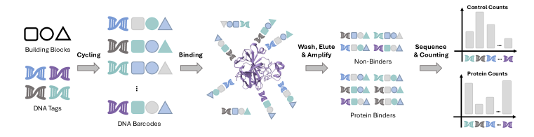
DNA-encoded library (DEL) technology has emerged as a revolutionary approach for protein-ligand binding detection, offering unprecedented advantages over traditional high-throughput screening methods(Franzini et al., 2014; Neri & Lerner, 2018; Peterson & Liu, 2023; Ma et al., 2023). The DEL screening process involves multiple stages including cycling, binding, washing, elution, and amplification (as shown in Figure 1). This process generates large-scale read count data, serving as a proxy for potential binding affinity(Machutta et al., 2017; Foley et al., 2021). The read counts represent the frequency of each compound in the selected pool after undergoing target protein binding and subsequent processing steps (Favalli et al., 2018). These read counts typically include control counts and protein counts, representing values corresponding to the scenarios without and with specific protein targets, respectively.
DEL screening enables the rapid and cost-effective evaluation of vast chemical spaces, typically encompassing billions of compounds (Satz et al., 2022), against biological targets of interest (Neri & Lerner, 2017). This approach has gained widespread adoption in drug discovery due to its ability to identify novel chemical scaffolds and accelerate lead compound identification (Brenner & Lerner, 1992; Goodnow Jr & Davie, 2017; Yuen & Franzini, 2017). This study aims to enhance the correlation between predicted read counts and true binding affinity. However, DEL screening read counts are subject to , stemming from both experimental variabilities and intrinsic factors (Favalli et al., 2018). These noisy elements introduce discrepancies between read counts and experimentally determined values (Yung-Chi & Prusoff, 1973), which represent the binding affinity of a ligand to its target protein in the training data, making this task highly challenging.
To mitigate noise, researchers apply threshold-based filtering to enrichment factors, calculated as the ratio of protein count to control count(Gu et al., 2008; Kuai et al., 2018), to classify compounds as potential hits or noise(Gu et al., 2008; Kuai et al., 2018). Although these methods offer advantages in interpretability and computational efficiency, they focus solely on the inherent properties of read counts, overlooking the complex relationships between ligand molecular structures and their corresponding read counts(McCloskey et al., 2020). To address this limitation, researchers leveraged machine learning techniques to capture the non-linear relationships between ligand molecules and their count labels, aiming to predict more accurate read counts (McCloskey et al., 2020; Ma et al., 2021). These approaches, while more sophisticated in modeling molecular features, initially did not consider the constraints at the read count distribution level. Recognizing this gap, researchers further advanced the field by unifying both molecular structure-based predictions and distribution-level constraints. They developed methods incorporating distribution consistency losses, which use ligand sequence embedding to predict enrichment factors and evaluate the consistency of protein and control counts (Lim et al., 2022; Hou et al., 2023).
Recognizing the limitations of 2D ligand sequences in capturing spatial information, DEL-Dock (Shmilovich et al., 2023) introduced protein-ligand 3D conformational information to enhance denoising. However, compared to exploring different dimensional representations of ligands, enrichment factors only focus on the absolute values of ligand-corresponding read counts, neglecting their relative ordering, which is more stable and reliable, especially with experimental noise and systematic errors. Moreover, read counts primarily reflect the enrichment degree of compounds in the screening process but do not directly represent the biological activity of compounds. Without incorporating the activity information, models may overlook important ligand-activity relationships.
To address these multifaceted challenges, we propose a novel denoising framework that integrates a theoretically grounded combined ranking loss with an iterative validation loop for read count distribution correction. We introduce two novel constraints: the Pair-wise Soft Rank (PSR) and List-wise Global Rank (LGR). These constraints enable simultaneous learning of local discriminative features and global patterns in read count distributions. By emphasizing the relative relationships between compounds while integrating point-wise constraints based on their absolute read count values, our method provides a comprehensive approach to modeling the complex distributions in DEL. We prove that our novel ranking loss provides complementary information to ZIP loss and reduces the expected error bound, thereby ensuring the reliability of our algorithm.
Considering the ligand-activity relationships for distribution correction, we introduce a novel activity label derived from the analysis of functional groups in the DEL library’s ligands. This innovation forms the foundation of our proposed Activity-Referenced Distribution Correction (ARDC) framework. ARDC is designed to optimize the correlation between predicted read count values and potential binding affinities. It incorporates two key components: Iterative Activity-Guided Refinement (AGR) and Consistency-Driven Error Correction (CDEC). The AGR process, inspired by self-training techniques (Zoph et al., 2020), iteratively refines predictions by adjusting the model based on evolving read count to binding affinity relationships. CDEC addresses potential error accumulation through a consistency loss function, aligning predictions with biological reality and resolving discrepancies between the read counts and the activity levels.
To address the information gap in existing open-source datasets, we introduce three comprehensive datasets incorporating ligand 2D sequences, 3D structures, and corresponding activity labels. These datasets establish new benchmarks for denoising DEL libraries. To validate our approach, we conducted extensive experiments on five diverse DEL datasets. Our results demonstrate state-of-the-art performance across various correlation metrics, with comprehensive ablation studies underscoring the superiority of our distribution correction method. This work represents a significant advancement towards more accurate and reliable binding affinity predictions from DEL screening data, potentially accelerating drug discovery and enhancing the identification of potent lead compounds.
2 Related Works
Traditional DEL data analysis approaches, like QSAR models (Martin et al., 2017) and molecular docking simulations (Jiang et al., 2015; Wang et al., 2015), offer interpretability and mechanistic insights. DEL-specific methods such as data aggregation (Satz, 2016) and normalized z-score metrics (Faver et al., 2019) address unique DEL screening challenges. However, these methods face limitations in scalability and handling complex, non-linear relationships in large-scale DEL datasets.
Machine learning techniques such as Random Forest, Gradient Boosting Models, and Support Vector Machines have improved DEL data analysis (Li et al., 2018; Ballester & Mitchell, 2010). Combined with Bayesian Optimization (Hernández-Lobato et al., 2017), these methods offer better scalability and capture complex, non-linear relationships in high-dimensional DEL data. Despite outperforming traditional methods, they are limited by their reliance on extensive training data and lack of interpretability in complex biochemical systems.
Deep learning approaches, particularly Graph Neural Networks (GNNs), have significantly advanced protein-ligand interaction predictions in DEL screening. GNN-based models predict enrichment scores and accommodate technical variations (Stokes et al., 2020; Ma et al., 2021), while Graph Convolutional Neural Networks (GCNNs) enhance detection of complex molecular structures (McCloskey et al., 2020; Hou et al., 2023). Recent innovations include DEL-Dock, combining 3D pose information with 2D molecular fingerprints (Shmilovich et al., 2023), and sparse learning methods addressing noise from truncated products and sequencing errors (Kómár & Kalinic, 2020). Large-scale prospective studies have validated these AI-driven approaches, confirming improved hit rates and specific inhibitory activities against protein targets (Gu et al., 2024).
While existing methods offer improved scalability and the ability to capture complex molecular interactions, they still face challenges in interpretability. Moreover, they often lack a robust theoretical foundation for handling the unique characteristics of DEL read count data, particularly in terms of ranking and distribution correction. The persistent issues of Distribution Noise and Distribution Shift in DEL data remain inadequately addressed by current approaches.
To address these limitations, we propose a novel denoising framework that integrates a theoretically grounded combined ranking loss with an iterative validation loop. This approach aims to correct read count distributions more effectively, addressing both Distribution Noise and Distribution Shift, while improving the interpretability and reliability of binding affinity predictions in DEL screening.
3 Method
We present DEL-Ranking framework that directly denoises DEL read count values and incorporates new activity information. In Section 3.1, we directly formulate the problem. Sections 3.2 and 3.3 detail our innovative modules, while Section 3.4 introduces the overall training objective.
3.1 Problem Formulation and preliminaries
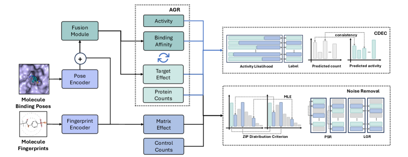
DEL Prediction Framework. Given a DEL dataset , where denotes the molecular fingerprint, represents the binding pose, is the matrix count derived from control experiments without protein targets, is the target count obtained from experiments involving protein target binding, and indicates the activity label. We propose a joint multi-task learning framework such that:
| (1) |
where represents the predicted matrix count, denotes the predicted target count, and is the predicted activity likelihood. The primary focus of this framework lies in predicting accurate read count values that strongly correlate with the actual values.
Zero-Inflated Distribution. DEL screening often results in read count distributions with a high proportion of zeros due to experimental factors. To address this, previous methods (Shmilovich et al., 2023; Lim et al., 2022) have employed zero-inflated distributions, modeling read counts as (, ), where accounts for excess zeros and represents non-zero counts.
| (2) |
where denotes the probability of excess zeros, represents the mean of the negative binomial distribution, and is the dispersion parameter.
Estimation. DEL read count prediction ultimately aims to estimate compound-target binding affinities ( values), crucial for identifying promising drug candidates. We evaluate our model’s effectiveness using the Spearman rank correlation coefficient () between predicted read counts and true values: where is the sample number and is the ranking discrepancy between predictions and true values. Ideally, values and read counts are negatively correlated.
3.2 Ranking-based Distribution Noise Removal
To effectively remove Distribution Noise in DEL read count data, we propose a novel ranking-based loss function . This loss function integrates both local and global read count information to achieve a well-ordered Zero-Inflated Poisson distribution for read count values:
| (3) |
where is a balancing hyperparameter. (Pairwise-Soft Ranking Loss) addresses local pairwise comparisons, while (listwise Global Ranking Loss) captures global ranking information. Together, they aim to achieve a well-ordered Zero-Inflated Poisson distribution for read count values. To formally establish the effectiveness of our ranking-based approach, we provide the following theoretical justification:
Lemma 1.
Given a set of feature-read count pairs , where is the fused representation of sample based on and , and a well-fitted Zero-Inflated Poisson model , the ranking loss provides positive information gain over the zero-inflated loss :
where denotes the conditional entropy of read counts .
Building upon this information gain, we can further demonstrate that our combined approach, which incorporates both the zero-inflated and ranking losses, outperforms the standard zero-inflated model in terms of expected loss. This improvement is formalized in the following theorem:
Theorem 2.
Given a sufficiently large dataset of feature-read count pairs, let be the loss function of standard zero-inflated model and be the combined ranking loss. For predictions and from the standard and combined models respectively. Define , there exists such that:
The incorporated ranking information aligns read count across compounds, mitigating experimental biases in DEL screening data. Detailed proof and analysis are provided in Sections A.1 and A.2.
3.2.1 Pairwise Soft Ranking Loss
To address the challenges of modeling relative discrete connections between compound pairs and remove read count Distribution Noise, we propose the differentiable Pairwise Soft Ranking loss . This novel loss function is designed to capture fine-grained ranking information while maintaining smooth gradients for stable optimization. is expressed as follows:
| (4) | ||||
where represents the predicted read count value for compound . To ensure smooth gradients and numerical stability, we introduce a scaling factor with temperature , allowing for fine-tuned control over the ranking sensitivity.
To accurately capture the impact of ranking changes, we design to approximate the relative importance of swapping compounds and . We introduce a gain function and a rank-based discount function , where is a small constant for numerical stability. These smooth functions ensure stable gradients during optimization.
To further normalize the impact of ranking changes, we compute a normalization factor in :
| (5) |
where is the k-th element of the descending-sorted y. This factor adapts our loss to varying dataset sizes and read count distributions, enhancing the robustness of our ranking model.
3.2.2 listwise Global Ranking Loss
To further consider global order in compound ranking, we propose the listwise Global Ranking (LGR) loss as a complement to the Pairwise Soft Ranking loss , which is expressed as :
| (6) |
where is the true ranking permutation of the compounds; is a temperature parameter for score rescaling to sharpen the predicted distribution, and denotes a contrastive loss among ranking scores to capture local connections, and denotes the weight. This formulation is designed to achieve two critical objectives in DEL experiments: (1) Near-deterministic selection of compounds with the highest read counts, corresponding to the highest binding affinities; (2) Increased robustness to small noise perturbations in the experimental data. As approaches 0, our model becomes increasingly selective towards high-affinity compounds while maintaining resilience against common experimental noises. This dual optimization leads to more consistent identification of promising drug candidates and enhanced reliability in the face of experimental variability.
Despite the strengths of and , they struggle to differentiate activity levels among compounds with identical read count values, particularly those affected by experimental noise. This limitation can lead to misclassification of high-activity samples with artificially low read counts as truly low-activity samples. To address this critical issue, we introduce a novel contrastive loss function , designed to enhance discrimination between varying levels of biological activity, especially for samples with zero or identical read count values. Let be a ranking function and a fixed threshold. We define as:
| (7) |
This loss function is positive if and only if , enforcing a minimum margin between differently ranked samples. The constant gradients and for promote robust ranking relationships.
3.3 Activity-Referenced Distribution Correction Framework
To effectively leverage activity information and address distribution shifts in DEL experiments, we propose the Activity-Referenced Distribution Correction (ARDC) framework. This approach reinforces the impact of activity labels on read count distributions through two key components: Iterative Activity-Guided Refinement (AGR) and Consistency-Driven Error Correction (CDEC).
The Iterative Activity-Guided Refinement process incorporates activity information into read count predictions. Detailed in Algorithm 1, this process handles matrix counts and target counts separately. Matrix counts are predicted using 2D SMILES embeddings, while target counts leverage 2D-3D joint embeddings. An adaptive iterative mechanism, inspired by self-training techniques in semi-supervised learning (Zoph et al., 2020), progressively improves the consistency between read count predictions and activity labels. This recursive updating approach reinforces the influence of activity labels on read count values, ultimately converging towards more biologically consistent results.
To address potential error accumulation and further align predictions with biological reality, we introduce the Consistency-Driven Error Correction component. This feature utilizes a consistency loss function that not only regresses the predicted values but also aligns their trends with activity labels. This approach helps resolve discrepancies between compounds with low read counts but high activity. The consistency loss is defined as:
| (8) |
where and denote the predicted and ground-truth activity, respectively, while and represent the normalized predicted and ground-truth read count values between 0 and 1.
3.4 Total Training Objective
The total training objective integrates three distinct components. The zero-inflated distribution loss models the overall read count distribution, while the combined ranking loss refines the predicted ZIP distribution based on ordinal relationships. Additionally, the consistency loss further adjusts the distribution using activity labels. These components are combined into the total loss function as follows:
| (9) |
where and are weighting factors for the ranking and consistency losses, respectively.
4 Experiment
Datasets. CA9 Dataset: From the original data containing 108,529 DNA-barcoded molecules targeting human carbonic anhydrase IX (CA9) (Gerry et al., 2019), we derived two separate datasets. The first, denoted as 5fl4-9p, uses 9 docked poses that we generated ourselves. The second, 5fl4-20p, employs 20 docked poses using the 5fl4 structure. Both datasets lack activity labels. CA2 and CA12 Datasets From the CAS-DEL library (Hou et al., 2023), we generated three datasets comprising 78,390 molecules selected from 7,721,415 3-cycle peptide compounds. We performed docking to create 9 poses per molecule for each dataset. The CA2-derived dataset uses the 3p3h PDB structure (denoted as 3p3h), while two CA12-derived datasets use the 4kp5 PDB structure: 4kp5-A for normal expression and 4kp5-OA for overexpression. Binary affinity labels (0/1) are assigned based on a specific building block (BB3-197). Validation Dataset from ChEMBL (Zdrazil et al., 2024) includes 12,409 small molecules with affinity measurements for CA9, CA2, and CA12. Molecules have compatible atom types, molecular weights from 25 to 1000 amu, and inhibitory constants (Ki) from 90 pM to 0.15 M. A subset focusing on the 10-90th percentile range of the training data’s molecular weights provides a more challenging test scenario.
Evaluation Metrics and Hyperparameters. To evaluate our framework’s effectiveness, we employ two Spearman correlation metrics on the ChEMBL dataset (Zdrazil et al., 2024). The first metric, overall Spearman correlation (), measures the correlation between predicted read counts and experimentally determined values across the entire validation dataset. Also, we utilize the subset Spearman correlation (), which focuses on compounds with molecular weights within the 10th to 90th percentile range of the training dataset. Hyperparameters setting is shown in Appendix A.3.
Baselines. We examine the performance of existing binding affinity predictors. Traditional methods based on binding poses and fingerprints inculde Molecule Weight, Benzene Sulfonamide, Vina Docking (Koes et al., 2013), and Dos-DEL(Gerry et al., 2019). AI-aided methods dependent of read count values and molecule information include DEL-QSVR, and DEL-Dock (Lim et al., 2022; Shmilovich et al., 2023). All methods are tested on 5 different target datasets.
4.1 Performance Comparison
| 3p3h (CA2) | 4kp5-A (CA12) | 4kp5-OA (CA12) | ||||
|---|---|---|---|---|---|---|
| Metric | Sp | SubSp | Sp | SubSp | Sp | SubSp |
| Mol Weight | -0.250 | -0.125 | -0.101 | 0.020 | -0.101 | 0.020 |
| Benzene | 0.022 | 0.072 | -0.054 | 0.035 | -0.054 | 0.035 |
| Vina Docking | -0.174±0.002 | -0.017±0.003 | 0.025±0.001 | 0.150±0.003 | 0.025±0.001 | 0.150±0.003 |
| Dos-DEL | -0.048±0.036 | -0.011±0.035 | -0.016±0.029 | -0.017±0.021 | -0.003±0.030 | -0.048±0.034 |
| DEL-QSVR | -0.228±0.021 | -0.171±0.033 | -0.004±0.178 | 0.018±0.139 | 0.070±0.134 | -0.076±0.116 |
| DEL-Dock | -0.255±0.009 | -0.137±0.012 | -0.242±0.011 | -0.263±0.012 | 0.015±0.029 | -0.105±0.034 |
| DEL-Ranking | -0.286±0.002 | -0.177±0.005 | -0.268±0.012 | -0.277±0.016 | -0.289±0.025 | -0.233±0.021 |
Benchmark Comparison. We conducted comprehensive experiments across five diverse datasets: 3p3h, 4kp5-A, 4kp5-OA, and two variants of 5fl4. For each dataset, we performed five runs to ensure statistical robustness. As shown in Table 1-2, our method consistently achieves state-of-the-art results in both Spearman (Sp) and subset Spearman (SubSp) coefficients across all datasets.
Our analysis reveals several key insights: (1) Experimental Adaptability: DEL-Ranking shows consistent advantages across diverse datasets, with notable gains in challenging conditions. It maintains improvements even in lower-noise environments like purified protein datasets (3p3h and 5fl4), versatility highlighting DEL-Ranking’s adaptability to various experimental setups. (2) Noise Resilience: DEL-Ranking excels in high-noise scenarios, particularly in membrane protein experiments. Its exceptional results on the 4kp5 dataset, especially the challenging 4kp5-OA variant, demonstrate this. Where baseline methods struggle, our approach effectively distinguishes signal from noise in complex experimental conditions. (3) Structural Flexibility: Our approach effectively uses structural information, as shown in the 5fl4 dataset. Increasing poses from 9 to 20 improves model performance, highlighting our method’s ability to utilize additional structural data. This underscores DEL-Ranking’s effectiveness in extracting insights from comprehensive structural information. (4) Dual Analysis Capability: DEL-Ranking’s consistent performance in both Sp and SubSp metrics shows its versatility in drug discovery. This enables effective broad-spectrum screening and detailed subset analysis, enhancing its utility across various stages of drug discovery.
Zero-shot Generalization. We tested zero-shot generalization ability of DEL-Dock (Shmilovich et al., 2023) and DEL-Ranking on CA9 target, trained on 3p3h, 4kp5-A, and 4kp5-OA datasets. As shown in Table 3, DEL-Ranking consistently outperforms DEL-Dock across all datasets, demonstrating the robustness of our approach in diverse conditions. Notably, for the 4kp5-OA dataset, which likely contains higher experimental noise and poses significant challenges, DEL-Ranking shows a substantial improvement, revealing its enhanced robustness in handling noisy DEL data.
| 5fl4-9p (CA9) | 5fl4-20p (CA9) | |||
|---|---|---|---|---|
| Metric | Sp | SubSp | Sp | SubSp |
| Mol Weight | -0.121 | -0.028 | -0.121 | -0.074 |
| Benzene | -0.174 | -0.134 | -0.199 | -0.063 |
| Vina Docking | -0.114±0.009 | -0.055±0.007 | -0.279±0.044 | -0.091±0.061 |
| Dos-DEL | -0.115±0.065 | -0.036±0.010 | -0.231±0.007 | -0.091±0.012 |
| DEL-QSVR | -0.086±0.060 | -0.036±0.074 | -0.298±0.005 | -0.075±0.011 |
| DEL-Dock | -0.308±0.000 | -0.169±0.000 | -0.320±0.009 | -0.166±0.017 |
| DEL-Ranking | -0.323±0.015 | -0.175±0.000 | -0.330±0.007 | -0.187±0.013 |
4.2 Discovery of potential high affinity functional group
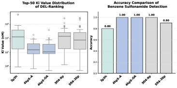
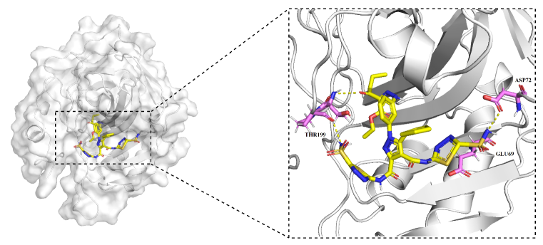
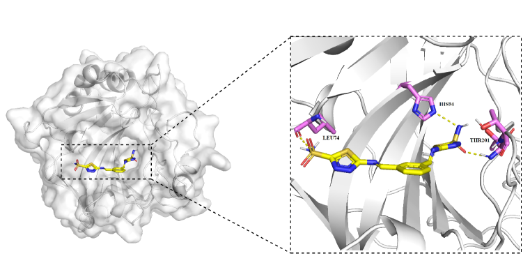
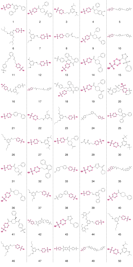
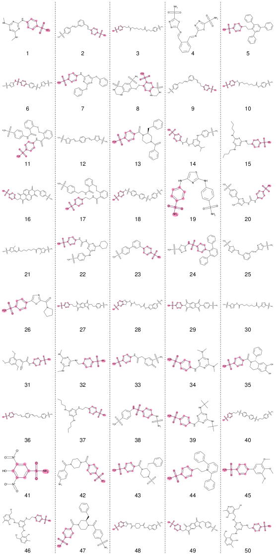
To assess DEL-Ranking’s ability in identifying high-affinity compounds and exploring potential functional groups, we analyzed Top-50 target count samples predicted by our model on five datasets. As shown in Figure 3, the majority of these samples demonstrated consistently low Ki values, validating the model’s effectiveness in prioritizing active compounds within large DEL libraries.
Known Group Accuracy. DEL-Ranking shows exceptional accuracy in detecting benzene sulfonamide, a key high-affinity group for carbonic anhydrase inhibitors (Hou et al., 2023). From Figure 3, we can observe that the model achieved high detection rates on five datasets, indicating effective incorporation of chemical space information through activity labels.
Novel Group Discovery Our analysis of the 3p3h and 5fl4 datasets revealed a significant finding: 20% (10/50) of high-ranking compounds in 3p3h and 10% (5/50) in 5fl4 lack the expected benzene sulfonamide group. Remarkably, all these compounds contain a common functional group - Pyrimidine Sulfonamide - which shares high structural similarity with benzene sulfonamide.
Further investigation through case-by-case Ki value determination yielded compelling results. Five compounds from 3p3h and five from 5fl4 containing pyrimidine sulfonamide exhibited values comparable to or even surpassing those of benzene sulfonamide-containing compounds. This finding profoundly validates DEL-Ranking’s dual capability: successfully incorporating activity label information, while simultaneously leveraging multi-level information along with integrated ranking orders to uncover potential high-activity functional groups. Notably, this discovery reveals DEL-Ranking’s ability to identify unexplored scaffolds, showing potential to improve compound prioritization and accelerate hit-to-lead optimization in early-stage drug discovery. Detailed visualization of Top-50 samples and selected Pyrimidine Sulfonamide cases are shown in Sections A.4 and A.5.
| 3p3h (CA2) | 4kp5-A (CA12) | 4kp5-OA (CA12) | ||||
| Metric | Sp | SubSp | Sp | SubSp | Sp | SubSp |
| DEL-Dock | -0.272±0.013 | -0.118±0.005 | -0.211±0.007 | -0.118±0.010 | 0.065±0.021 | -0.125±0.034 |
| DEL-Ranking | -0.310±0.005 | -0.120±0.011 | -0.228±0.010 | -0.127±0.018 | -0.300±0.026 | -0.129±0.021 |
4.3 Ablation Study
To further explore the effectiveness of our enhancement, we compare DEL-Ranking with some variants on 3p3h, 4kp5-A, and 4kp5-OA datasets. We can observe from Table 4 that (1) and contribute most significantly to model performance across all datasets. (2) The impact of is more pronounced in datasets with higher noise levels, as evidenced by the larger relative performance drop in the 3p3h dataset. (3) Temperature adjustment and help improve the performance by correcting the predicted distributions, but count less than ranking-based denoising.
| 3p3h (CA2) | 4kp5-A (CA12) | 4kp5-OA (CA12) | ||||||||||
|---|---|---|---|---|---|---|---|---|---|---|---|---|
| Metric | Sp | SubSp | Sp | SubSp | Sp | SubSp | ||||||
| w/o All | -0.255 | 0.004 | -0.137 | 0.012 | -0.242 | 0.011 | -0.263 | 0.012 | 0.015 | 0.029 | -0.105 | 0.034 |
| w/o PSR | -0.273 | 0.012 | -0.155 | 0.013 | -0.251 | 0.015 | -0.271 | 0.011 | 0.015 | 0.028 | -0.105 | 0.033 |
| w/o LGR | -0.280 | 0.011 | -0.168 | 0.015 | -0.256 | 0.023 | -0.273 | 0.016 | -0.269 | 0.024 | -0.209 | 0.034 |
| w/o LGR-con | -0.283 | 0.004 | -0.172 | 0.007 | -0.260 | 0.018 | -0.273 | 0.014 | -0.273 | 0.024 | -0.218 | 0.034 |
| w/o Temp | -0.279 | 0.011 | -0.166 | 0.015 | -0.247 | 0.022 | -0.265 | 0.014 | -0.256 | 0.033 | -0.181 | 0.046 |
| w/o ARDC | -0.284 | 0.007 | -0.174 | 0.010 | -0.260 | 0.015 | -0.272 | 0.012 | -0.269 | 0.023 | -0.223 | 0.045 |
| DEL-Ranking | -0.286 | 0.002 | -0.177 | 0.005 | -0.268 | 0.012 | -0.277 | 0.016 | -0.289 | 0.025 | -0.233 | 0.021 |
5 Conclusion
In this paper, we propose DEL-Ranking to addresses the challenge of noise in DEL screening through innovative ranking loss and activity-based correction algorithms. Experimental results demonstrate significant improvements in binding affinity prediction and generalization capability. Besides, the ability to identify potential binding affinity determinants advances the field of DEL screening analysis. Current limitations revolve around the challenges of acquiring, integrating, and comprehensively analyzing high-quality multi-modal molecular data at scale. Future works will aim to improve multi-modal data integration and analysis to advance DEL-based drug discovery.
References
- Ballester & Mitchell (2010) Pedro J Ballester and John BO Mitchell. A machine learning approach to predicting protein–ligand binding affinity with applications to molecular docking. Bioinformatics, 26(9):1169–1175, 2010.
- Brenner & Lerner (1992) Sydney Brenner and Richard A Lerner. Encoded combinatorial chemistry. Proceedings of the National Academy of Sciences, 89(12):5381–5383, 1992.
- Favalli et al. (2018) Nicolas Favalli, Gabriele Bassi, Jörg Scheuermann, and Dario Neri. Dna-encoded chemical libraries: achieving the screenable chemical space. FEBS letters, 592(12):2168–2180, 2018.
- Faver et al. (2019) John C Faver, Kevin Riehle, David R Lancia Jr, Jared BJ Milbank, Christopher S Kollmann, Nicholas Simmons, Zhifeng Yu, and Martin M Matzuk. Quantitative comparison of enrichment from dna-encoded chemical library selections. ACS combinatorial science, 21(2):75–82, 2019.
- Foley et al. (2021) Timothy L Foley, Woodrow Burchett, Qiuxia Chen, Mark E Flanagan, Brendon Kapinos, Xianyang Li, Justin I Montgomery, Anokha S Ratnayake, Hongyao Zhu, and Marie-Claire Peakman. Selecting approaches for hit identification and increasing options by building the efficient discovery of actionable chemical matter from dna-encoded libraries. SLAS DISCOVERY: Advancing the Science of Drug Discovery, 26(2):263–280, 2021.
- Franzini et al. (2014) Raphael M Franzini, Dario Neri, and Jorg Scheuermann. Dna-encoded chemical libraries: advancing beyond conventional small-molecule libraries. Accounts of chemical research, 47(4):1247–1255, 2014.
- Gerry et al. (2019) Christopher J Gerry, Mathias J Wawer, Paul A Clemons, and Stuart L Schreiber. Dna barcoding a complete matrix of stereoisomeric small molecules. Journal of the American Chemical Society, 141(26):10225–10235, 2019.
- Goodnow Jr & Davie (2017) Robert A Goodnow Jr and Christopher P Davie. Dna-encoded library technology: a brief guide to its evolution and impact on drug discovery. In Annual Reports in Medicinal Chemistry, volume 50, pp. 1–15. Elsevier, 2017.
- Gu et al. (2024) Chunbin Gu, Mutian He, Hanqun Cao, Guangyong Chen, Chang-yu Hsieh, and Pheng Ann Heng. Unlocking potential binders: Multimodal pretraining del-fusion for denoising dna-encoded libraries. arXiv preprint arXiv:2409.05916, 2024.
- Gu et al. (2008) Kangxia Gu, Hon Keung Tony Ng, Man Lai Tang, and William R Schucany. Testing the ratio of two poisson rates. Biometrical Journal: Journal of Mathematical Methods in Biosciences, 50(2):283–298, 2008.
- Hernández-Lobato et al. (2017) José Miguel Hernández-Lobato, James Requeima, Edward O Pyzer-Knapp, and Alán Aspuru-Guzik. Bayesian optimization for synthetic gene design. arXiv preprint arXiv:1712.07037, 2017.
- Hou et al. (2023) Rui Hou, Chao Xie, Yuhan Gui, Gang Li, and Xiaoyu Li. Machine-learning-based data analysis method for cell-based selection of dna-encoded libraries. ACS omega, 2023.
- Jiang et al. (2015) Hao Jiang, Connor W Coley, and William H Green. Advances in the application of molecular docking for the design of dna-encoded libraries. Journal of chemical information and modeling, 55(7):1297–1308, 2015.
- Koes et al. (2013) David Ryan Koes, Matthew P Baumgartner, and Carlos J Camacho. Lessons learned in empirical scoring with smina from the csar 2011 benchmarking exercise. Journal of chemical information and modeling, 53(8):1893–1904, 2013.
- Kómár & Kalinic (2020) Péter Kómár and Marko Kalinic. Denoising dna encoded library screens with sparse learning. ACS Combinatorial Science, 22(8):410–421, 2020.
- Kuai et al. (2018) Letian Kuai, Thomas O’Keeffe, and Christopher Arico-Muendel. Randomness in dna encoded library selection data can be modeled for more reliable enrichment calculation. SLAS DISCOVERY: Advancing the Science of Drug Discovery, 23(5):405–416, 2018.
- Li et al. (2018) Jiao Li, Aoqin Fu, and Le Zhang. Machine learning approaches for predicting compounds that interact with therapeutic and admet related proteins. Journal of pharmaceutical sciences, 107(6):1543–1553, 2018.
- Lim et al. (2022) Katherine S Lim, Andrew G Reidenbach, Bruce K Hua, Jeremy W Mason, Christopher J Gerry, Paul A Clemons, and Connor W Coley. Machine learning on dna-encoded library count data using an uncertainty-aware probabilistic loss function. Journal of chemical information and modeling, 62(10):2316–2331, 2022.
- Ma et al. (2023) Peixiang Ma, Shuning Zhang, Qianping Huang, Yuang Gu, Zhi Zhou, Wei Hou, Wei Yi, and Hongtao Xu. Evolution of chemistry and selection technology for dna-encoded library. Acta Pharmaceutica Sinica B, 2023.
- Ma et al. (2021) Ralph Ma, Gabriel HS Dreiman, Fiorella Ruggiu, Adam Joseph Riesselman, Bowen Liu, Keith James, Mohammad Sultan, and Daphne Koller. Regression modeling on dna encoded libraries. In NeurIPS 2021 AI for Science Workshop, 2021.
- Machutta et al. (2017) Carl A Machutta, Christopher S Kollmann, Kenneth E Lind, Xiaopeng Bai, Pan F Chan, Jianzhong Huang, Lluis Ballell, Svetlana Belyanskaya, Gurdyal S Besra, David Barros-Aguirre, et al. Prioritizing multiple therapeutic targets in parallel using automated dna-encoded library screening. Nature communications, 8(1):16081, 2017.
- Martin et al. (2017) Eric J Martin, Valery R Polyakov, Lan Zhu, and Lu Zhao. Quantitative analysis of molecular recognition in dna-encoded libraries. Journal of chemical information and modeling, 57(9):2077–2088, 2017.
- McCloskey et al. (2020) Kevin McCloskey, Eric A Sigel, Steven Kearnes, Ling Xue, Xia Tian, Dennis Moccia, Diana Gikunju, Sana Bazzaz, Betty Chan, Matthew A Clark, et al. Machine learning on dna-encoded libraries: a new paradigm for hit finding. Journal of Medicinal Chemistry, 63(16):8857–8866, 2020.
- Neri & Lerner (2017) Dario Neri and Richard A Lerner. Dna-encoded chemical libraries: a selection system based on endowing organic compounds with amplifiable information. Annual review of biochemistry, 86:813–838, 2017.
- Neri & Lerner (2018) Dario Neri and Richard A Lerner. Dna-encoded chemical libraries: a selection system based on endowing organic compounds with amplifiable information. Annual review of biochemistry, 87:479–502, 2018.
- Peterson & Liu (2023) Alexander A Peterson and David R Liu. Small-molecule discovery through dna-encoded libraries. Nature Reviews Drug Discovery, 22(9):699–722, 2023.
- Satz (2016) Alexander L Satz. Simulated screens of dna encoded libraries: the potential influence of chemical synthesis fidelity on interpretation of structure–activity relationships. ACS combinatorial science, 18(7):415–424, 2016.
- Satz et al. (2022) Alexander L Satz, Andreas Brunschweiger, Mark E Flanagan, Andreas Gloger, Nils JV Hansen, Letian Kuai, Verena BK Kunig, Xiaojie Lu, Daniel Madsen, Lisa A Marcaurelle, et al. Dna-encoded chemical libraries. Nature Reviews Methods Primers, 2(1):3, 2022.
- Shmilovich et al. (2023) Kirill Shmilovich, Benson Chen, Theofanis Karaletsos, and Mohammad M Sultan. Del-dock: Molecular docking-enabled modeling of dna-encoded libraries. Journal of Chemical Information and Modeling, 63(9):2719–2727, 2023.
- Stokes et al. (2020) Jonathan M Stokes, Kevin Yang, Kyle Swanson, Wengong Jin, Andres Cubillos-Ruiz, Nina M Donghia, Craig R MacNair, Shawn French, Lindsey A Carfrae, Zohar Bloom-Ackermann, et al. Deep learning-based prediction of protein–ligand interactions. Proceedings of the National Academy of Sciences, 117(32):19338–19348, 2020.
- Wang et al. (2015) Lingle Wang, Yujie Wu, Yuqing Deng, Byungchan Kim, Levi Pierce, Goran Krilov, Dmitry Lupyan, Shaughnessy Robinson, Markus K Dahlgren, Jeremy Greenwood, et al. Accurate and reliable prediction of relative ligand binding potency in prospective drug discovery by way of a modern free-energy calculation protocol and force field. Journal of the American Chemical Society, 137(7):2695–2703, 2015.
- Yuen & Franzini (2017) Lik Hang Yuen and Raphael M Franzini. Dna-encoded chemical libraries: advances and applications. Pflügers Archiv-European Journal of Physiology, 469:213–225, 2017.
- Yung-Chi & Prusoff (1973) Cheng Yung-Chi and William H Prusoff. Relationship between the inhibition constant (ki) and the concentration of inhibitor which causes 50 per cent inhibition (i50) of an enzymatic reaction. Biochemical pharmacology, 22(23):3099–3108, 1973.
- Zdrazil et al. (2024) Barbara Zdrazil, Eloy Felix, Fiona Hunter, Emma J Manners, James Blackshaw, Sybilla Corbett, Marleen de Veij, Harris Ioannidis, David Mendez Lopez, Juan F Mosquera, et al. The chembl database in 2023: a drug discovery platform spanning multiple bioactivity data types and time periods. Nucleic acids research, 52(D1):D1180–D1192, 2024.
- Zoph et al. (2020) Barret Zoph, Golnaz Ghiasi, Tsung-Yi Lin, Yin Cui, Hanxiao Liu, Ekin Dogus Cubuk, and Quoc Le. Rethinking pre-training and self-training. Advances in neural information processing systems, 33:3833–3845, 2020.
Appendix A Appendix
A.1 Proof of Lemma and Theorem
Proof.
[Proof of Lemma1] Let be a probability space and be random variables representing features and read counts respectively. Define as the probability mass function of a well-fitted Zero-Inflated Poisson model.
Define:
where is the observed dataset and .
We aim to prove , where denotes conditional mutual information.
Consider with . It’s possible that due to the nature of likelihood optimization in the ZIP model.
In this case:
This implies:
Consequently:
Therefore, . ∎
Proof.
[Proof of Theorem2] Given Lemma1, We firstly prove that there exists a set of predictions and a sufficiently small such that for all :
Define the combined loss function , where . Let be the minimizer of :
By the definition of , for any , we have:
Expanding this inequality:
Let and . Rearranging the inequality:
Given that , provides information not captured by . This implies that there exists such that for all , .
Now, consider the function:
We know that for all from the earlier inequality. Moreover, due to the information gain assumption.
By the continuity of , there exists such that for all :
This implies:
Dividing both sides by (which is positive for ):
This is equivalent to:
Substituting back the definitions of and :
Let , we have:
Rearranging this inequality:
The left-hand side of this inequality is by definition. The right-hand side is strictly greater than since for any non-trivial ranking loss and .
Therefore:
This completes the proof. ∎
A.2 Gradient Analysis
We analyze the composite ranking loss function , which combines Pairwise Soft Ranking Loss and Listwise Global Ranking Loss. The gradient of with respect to is:
| (10) |
| (11) |
where
| (12) |
The gradient is primarily determined by and , which represent pairwise comparisons between item and other items . captures the NDCG impact of swapping items and , while adjusts this impact based on the difference between and . This formulation ensures that focuses on local ranking relationships, particularly between adjacent or nearby items.
| (13) |
The gradient incorporates information from all items ranked from position to . Through its softmax formulation, it considers the position of item relative to all items ranked below it. This allows to capture global ranking information.
A.3 Hyperparameter Setting
The model was trained using the Adam optimizer with mini-batches of 64 samples. The network architecture employed a hidden dimension of 128. The self-correction mechanism was applied for 3 iterations. All experiments were conducted on a single NVIDIA RTX 3090 GPU with 24GB memory. The implementation utilized PyTorch-Lightning version 1.9.0 to streamline the training process and enhance reproducibility. The hyperparameter settings for different datasets, including loss function weights, temperature, and margin, are detailed in Table 5.
| 3p3h | 4kp5-A | 4kp5-OA | 5fl4-9p | 5fl4-20p | |
|---|---|---|---|---|---|
| ARDC weight | 1 | 0.1 | 0.1 | – | – |
| PSR weight | |||||
| LGR weight | 1.0 | 0.1 | 0.1 | 2.0 | 1.0 |
| Temperature | 0.8 | 0.3 | 0.2 | 0.9 | 0.2 |
| Contrast weight | |||||
| Margin |
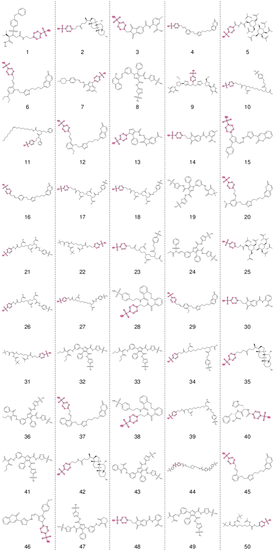
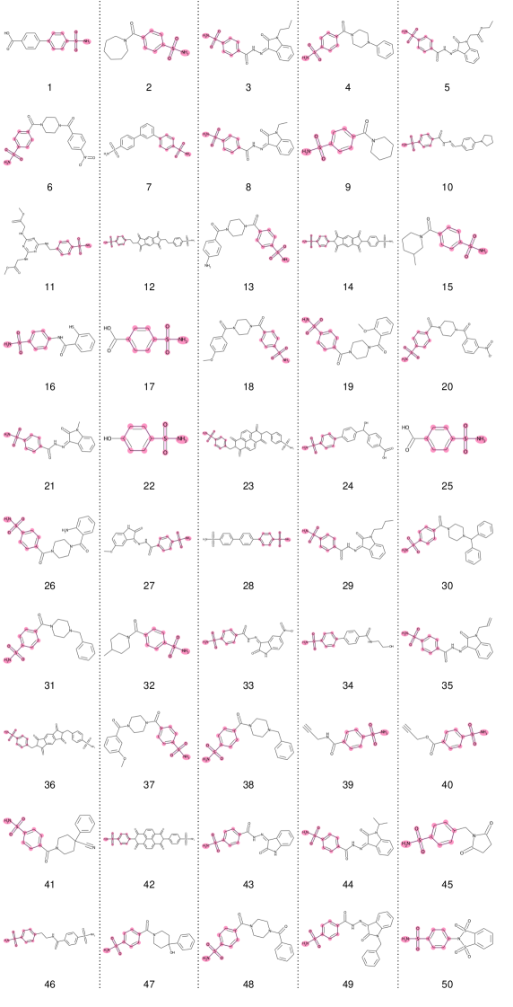
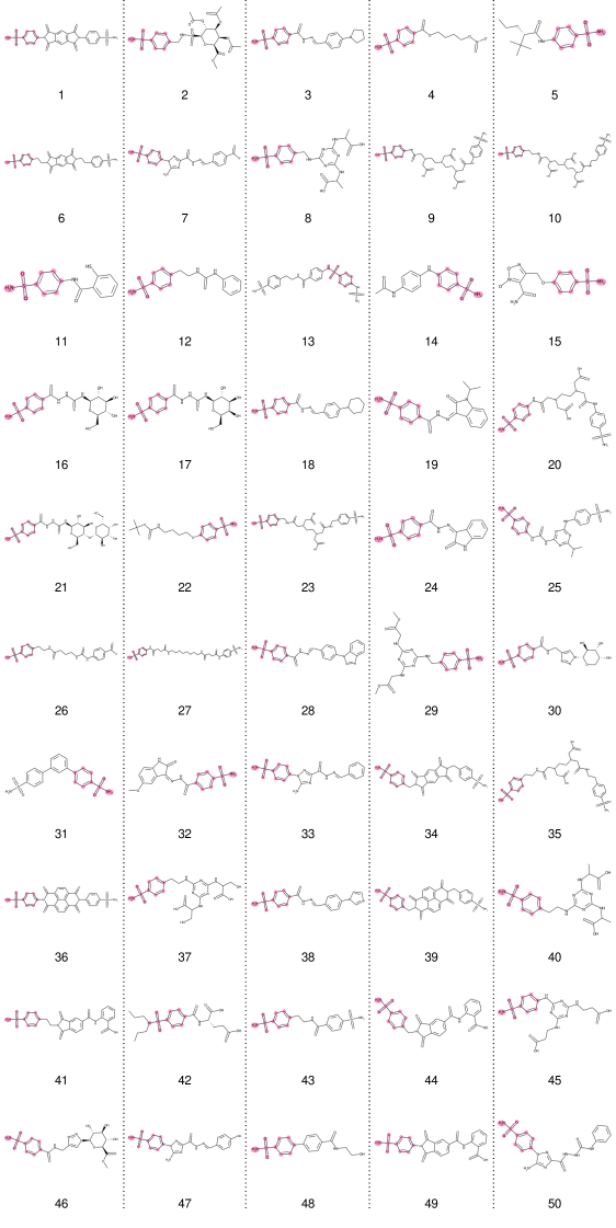
A.4 Visualization of Top-50 Selection
The visualization of the Top-50 DEL-Ranking results based on predicted target counts on five datasets are shown in Figure Figures 4, 5, 6, 8 and 7. We highlight the potential benzenesulfonamide structures in each sample using pink color.
A.5 Visualization on Selected Cases Containing Pyrimidine Sulfonamide