Abstract

Turbulence has remained the greatest challenge in fluid mechanics. Especially, randomness is one of the most important characteristics of turbulence, but its origin is still an open question until now. In this paper, by means of several ingeniously designed “clean” numerical experiments based on Navier-Stokes equations for the two-dimensional turbulent Kolmogorov flow, we reveal such a new phenomenon, namely “noise-expansion cascade”, that all micro-level noises/disturbances at different orders of magnitude in initial condition of Navier-Stokes equations enlarge consistently, say, one by one like an inverse cascade, to macro-level, and besides each of them might greatly change macro-level characteristic of turbulence. The “noise-expansion cascade” closely connects randomness of micro-level noise/disturbance and macro-level disorder of turbulence and thus reveals the origin of randomness of turbulence. In addition, it clearly indicates that unavoidable thermal fluctuation must be considered for turbulence, even if it is several orders of magnitude smaller than other external environmental disturbances.

Keyword turbulence, cascade, noise, randomness, clean numerical simulation

1 Motivation

“Turbulence is the last great unsolved problem of classical physics”, as pointed out by the Nobel Prize winner Richard Feynman. Especially, the randomness is one of the most important characteristics of turbulence [1], but its origin is still an open question until now, to the best of our knowledge.

Today it is widely accepted by scientific community that turbulent flows can be described mathematically by the Navier-Stokes (NS) equations. The NS equations are so important and fundamental that they become the fourth millennium problem [2] of Clay Mathematics Institute of Cambridge, Massachusetts. In 1970 Orszag [3] proposed the so-called “direct numerical simulation” (DNS), which numerically solved the NS equations without any turbulence modes. This is a milestone in fluid mechanics, since it opened the times of numerical experiment. DNS has become a useful tool in fundamental research of turbulence [4, 5, 6, 7, 8], and each result given by DNS has been regarded as a “clean” benchmark solution, because it is widely believed that numerical noise of DNS should not be enlarged to a macro-level due to the viscosity of fluid. As pointed out by Coleman and Sandberg [8], DNS has “the ability to perform fundamental studies of clean flows unaffected by numerical, modelling and measurement errors” and “the complete control of the initial and boundary conditions, and each term in the governing equations, also leads to profound advantages over laboratory and field studies.”

Let $f({\bf r})+\Delta_{1}({\bf r})+\Delta_{2}({\bf r})$ denote an initial condition of the NS equations, where ${\bf r}$ is a spatial vector, $f({\bf r})$ is a function at macro-level, $\Delta_{1}({\bf r})$ is a small disturbance at a micro-level, for example at the order $10^{-20}$ of magnitude, and $\Delta_{2}({\bf r})$ is an even smaller disturbance at a micro-level, for example at the order $10^{-40}$ of magnitude, respectively. Traditionally, it is widely believed that the 2nd disturbance $\Delta_{2}({\bf r})$ could be negligible since it is 20 orders of magnitude smaller than the first disturbance $\Delta_{1}({\bf r})$. Is this traditional viewpoint really correct for turbulent flow governed by NS equations? This is a fundamental problem, which, to the best of our knowledge, is still an open question, too.

Obviously, the above-mentioned two open questions have close relationships. In order to answer these open questions, it is necessary to develop a new kind of numerical algorithm, whose numerical noise must be much smaller than micro-level physical disturbances and artificial numerical noises of other traditional numerical algorithms throughout a long enough interval of time. In 2009 the so-called “clean numerical simulation” (CNS) was proposed by Liao [9] for chaos and turbulence, and since then its computational efficiency has been increased, step by step, several orders of magnitude [10, 11, 12, 13]. Unlike DNS, CNS algorithm uses multiple-precision [14] with a large enough number of significant digits and thus can decrease both of truncation error and round-off error to any required tiny level. Thus, numerical noise of CNS can be rigorously negligible throughout a time interval that is long enough for calculating statistics [10]. Therefore, CNS result is much more accurate than DNS in a finite but long enough interval of time and thus can be used as “clean” benchmark solution to check the validity of DNS.

For example, it was found [15] that the DNS result of a two-dimensional turbulent Rayleigh-Bénard (RB) convection, which is excited by a thermal fluctuation as initial condition, quickly departs from the corresponding CNS benchmark solution: it is a kind of non-shearing vortical/roll-like convection at the beginning but then quickly turns into a kind of zonal flow, while the CNS benchmark solution always remains the same non-shearing vortical/roll-like convection in a finite but long enough interval of time $t\in[0,T_{c}]$, where $T_{c}$, called “the critical predictable time”, is equal to 500 (i.e. $T_{c}=500$) for the RB convection under consideration. To further confirm this, a 2D turbulent Kolmogorov flow, which is excited by an initial condition with a spatial symmetry, was solved [16] by DNS and CNS, respectively. It was found [16] that the spatiotemporal trajectory of the CNS benchmark solution remains a kind of spatial symmetry throughout the whole interval of time [0,1000], however the spatiotemporal trajectory of the corresponding DNS result is the same at the beginning as the CNS benchmark result but quickly loses the spatial symmetry, clearly indicating that the spatio-temporal trajectory of the 2D turbulent Kolmogorov flow given by DNS is badly polluted by artificial numerical noise that quickly increases to the same order of magnitude as the exact solution of NS equations. It clearly illustrated that the 2D turbulent Kolmogorov flow [16] is a chaotic system, say, its spatio-temporal trajectory is rather sensitive to small disturbance caused by artificial numerical noise. More importantly, DNS result sometimes might have great deviations from CNS benchmark solution not only in flow type and/or spatial symmetry of flow field but also even in statistics, as illustrated in [15, 16]. These two successful applications of CNS illustrated that CNS can indeed provide us the ability to do such kind of “clean” numerical experiments that we can accurately investigate the evolution and propagation of micro-level noises/disturbances in initial condition of the NS equations for turbulence. It should be emphasized that this object cannot be realized by DNS whose numerical noise quickly increases to the same order of magnitude as true solution, as illustrated in [15, 16].

Note that CNS has been successfully used to attack some rather difficult problems in classical mechanics. For example, the number of periodic orbits of the famous three-body problem, which can be traced back to Newton in 1687, has been increased several orders of magnitude by means of CNS [17, 18, 19], because trajectories of three-body system are essentially chaotic, but CNS, unlike other traditional numerical methods, can correctly calculate its chaotic trajectory. Since three-body problem is very famous in history, the discoveries of these new periodic orbits have been reported twice by New Scientist [20, 21]. This is a good example to show the importance to gain accurate trajectory of some complicated dynamic systems.

In this paper, greatly inspired by spatial symmetry of the CNS benchmark solution of the 2D turbulent Kolmogorov flow [16], we ingeniously design several clean numerical experiments based on CNS for a two-dimensional (2D) turbulent Kolmogorov flow governed by NS equations with some specially chosen initial conditions that contain terms at different orders of magnitudes with different spatial symmetry so as to accurately investigate their propagations, evolutions, and also their macro-scale influences on the turbulence. These clean numerical experiments provide us a rigorous evidence that all noises/disturbances at different orders of magnitude in initial condition of NS equations could enlarge, one by one like an inverse cascade, to a macro-level, and in addition each of them could lead to great change to characteristic of turbulence. Based on this interesting phenomenon, a new concept, namely “noise-expansion cascade”, is proposed. The “noise-expansion cascade” closely connects randomness of micro-level noise/disturbance and macro-level disorder of turbulence, and thus reveals an origin of randomness of turbulence. Besides, according to “noise-expansion cascade”, unavoidable thermal fluctuation must be considered for turbulence, even if it is many orders of magnitudes smaller than other external disturbances.

The set up of the clean numerical experiments is described in § 2. The detailed results of the ingeniously designed clean numerical experiments are reported, and especially the phenomenon, called “noise-expansion cascade”, is revealed in § 3. The conclusions and discussions are given in § 4.

2 Set up of clean numerical experiment

Consider the 2D incompressible Kolmogorov flow [22, 23, 24] in a square domain $[0,L]^{2}$ (with a periodic boundary condition) under the so-called “Kolmogorov forcing”, which is stationary, monochromatic, and cosusoidally varying in space, with an integer $n_{K}$ describing the forcing scale and $\chi$ representing the corresponding forcing amplitude per unit mass of fluid, respectively. Using the length scale $L/2\pi$ and the time scale $\sqrt{L/2\pi\chi}$, the non-dimensional Navier-Stokes equation of this 2D Kolmogorov flow in the form of stream function reads

$$\frac{\partial}{\partial t}\Big{(}\nabla^{2}\psi\Big{)}+\frac{\partial(\psi,\nabla^{2}\psi)}{\partial(x,y)}-\frac{1}{Re}\nabla^{4}\psi+n_{K}\cos(n_{K}y)=0,$$ (1)

where

$$Re=\frac{\sqrt{\chi}}{\nu}\left(\frac{L}{2\pi}\right)^{\frac{3}{2}}$$

is the Reynolds number, $\nu$ denotes the kinematic viscosity, $\psi$ is the stream function, $x,y\in[0,2\pi]$ are horizontal and vertical coordinates, $t$ denotes the time, $\nabla^{2}$ is the Laplace operator, $\nabla^{4}=\nabla^{2}\nabla^{2}$, and

$$\frac{\partial(a,b)}{\partial(x,y)}=\frac{\partial a}{\partial x}\frac{\partial b}{\partial y}-\frac{\partial b}{\partial x}\frac{\partial a}{\partial y}$$

is the Jacobi operator, respectively. Note that the stream function $\psi$ always satisfies the periodic boundary condition

$$\psi(0,y,t)=\psi(2\pi,y,t),\hskip 8.5359pt\psi(x,0,t)=\psi(x,2\pi,t),\hskip 8.5359pt\mbox{for $x,y\in[0,2\pi],t\geq 0$}.$$ (2)

In order to have a relatively strong state of turbulent flow, we choose $n_{K}=16$ and $Re=2000$ for all cases considered in this paper.

Let us consider the following three different initial conditions

$$\psi(x,y,0) = -\frac{1}{2}\big{[}\cos(x+y)+\cos(x-y)\big{]},$$ (3)

$$\psi(x,y,0) = -\frac{1}{2}\big{[}\cos(x+y)+\cos(x-y)\big{]}+\delta^{\prime}\sin(x+y),$$ (4)

$$\psi(x,y,0) = -\frac{1}{2}\big{[}\cos(x+y)+\cos(x-y)\big{]}+\delta^{\prime}\sin(x+y)+\delta^{\prime\prime}\sin(x+2y),$$ (5)

respectively, where $\delta^{\prime}$ and $\delta^{\prime\prime}$ are constants, corresponding to a Kolmogorov flow with different spatial symmetry, as mentioned below.

Note that the initial condition (3) has the spatial symmetry

$$\left\{\begin{array}[]{ll}\mbox{rotation}&:\;\;\psi(x,y,t)=\psi(2\pi-x,2\pi-y,t),\\ \mbox{translation}&:\;\;\psi(x,y,t)=\psi(x+\pi,y+\pi,t),\end{array}\right.$$ (6)

at $t=0$. Here, we emphasize that Qin et al. [16] solved the 2D turbulent Kolmogorov flow governed by Eqs. (1) and (2) subject to the initial condition (3) in the case of $Re=40$ and $n_{K}=4$ by means of the DNS and the CNS, respectively. They found that the spatio-temporal trajectory given by DNS agrees well with the CNS benchmark solution from the beginning and remains the spatial symmetry (6) until $t\approx 120$ when the DNS result loses the spatial symmetry completely, but the CNS benchmark solution always remains the spatial symmetry (6) throughout the whole time interval $t\in[0,1500]$, clearly indicating that the spatio-temporal trajectory given by DNS is badly polluted by artificial numerical noise after $t\geq 120$. So, it is impossible to rigorously and accurately simulate the evolution and propagation of the micro-level disturbances by means of DNS. Thus, we had to give up DNS in this paper, but use CNS instead. More importantly, Qin et al. [16] revealed such an important fact that the 2D Kolmogorov turbulent flow given by CNS remains the same spatial symmetry as its initial condition: we will use this fact to do several ingeniously designed clean numerical experiments based on CNS, since the same conclusions about spatial symmetry should hold qualitatively for the case $n_{K}=16$ and $Re=2000$ considered in this paper.

The CNS algorithm is briefly described below. First of all, in order to decrease the spatial truncation error to a small enough level, we, like DNS, discretize the spatial domain of the flow field by a uniform mesh $N^{2}=1024^{2}$, and adopt the Fourier pseudo-spectral method for spatial approximation with the $3/2$ rule for dealiasing. In this way, the corresponding spatial resolution is fine enough for the considered Kolmogorov flow: the grid spacing is less than the average Kolmogorov scale, as mentioned in [25]. Besides, in order to decrease the temporal truncation error to a small enough level, we, unlike DNS, use the 140th-order (i.e. $M=140$) Taylor expansion with a time step $\Delta t=10^{-3}$. Furthermore, different from DNS, we use multiple-precision with 260 significant digits (i.e. $N_{s}=260$) for all physical/numerical variables and parameters so as to decrease the round-off error to a small enough level. In addition, the self-adaptive CNS strategy [13] and parallel computing are adopted to dramatically increase computational efficiency of the CNS algorithm. Especially, another CNS result is given by the same CNS algorithm but with even smaller numerical noises (say, using even larger $M$ and/or $N_{s}$ than those mentioned above), which confirms (by comparisons) that the numerical noise of the former CNS result (say, given by $N=1024,M=140,N_{s}=260$) are rigorously negligible throughout the whole interval $t\in[0,300]$ so that it can be used as a “clean” benchmark solution. For details, please refer to Qin et al. [16] and Liao’s book [10].

3 Results of clean numerical experiments

Our “clean” numerical experiments based on CNS have the following two stages:

1. At the first stage, we set $\delta^{\prime}=O(1)$ and $\delta^{\prime\prime}=O(1)$ in (4) and (5), and then confirm by means of CNS that the 2D turbulent Kolmogorov flow subject to the initial condition (3) or (4) always remains the same spatial symmetry as its corresponding initial condition, but the turbulent flow subject to the initial condition (5) has no spatial symmetry at all.

2. At the second stage, we set $\delta^{\prime}=10^{-20}$ and $\delta^{\prime\prime}=10^{-40}$ in (4) and (5), and then do the corresponding clean numerical experiments by means of CNS. The CNS results subject to the three different initial conditions (3),(4) and (5) are named by the flow CNS, the flow CNS^′ and the flow CNS^′′, respectively. The phenomenon, called “noise-expansion cascade”, is discovered by comparing the evolution of the spatial symmetry of these three kinds of turbulent flows.

Details of our clean numerical experiments based on CNS are described below.

3.1 Spatial symmetry under different initial conditions

First of all, Eqs. (1) and (2) subject to the initial condition (3) in the case of $Re=2000$ and $n_{K}=16$ are numerically solved by means of CNS. It is found that the CNS flow always remains the same spatial symmetry (6) throughout the whole time interval $t\in[0,300]$ exactly as the initial condition (3). This confirms the same conclusion about the spatial symmetry of the 2D Kolmogorov turbulent flow given by Qin et al. [16] using CNS in the different case of $Re=40$ and $n_{K}=4$. According to the governing equation (1), the periodic boundary condition (2), the initial condition (3) and the spatial symmetry (6), the corresponding solution should be in the following form of a series

$$\psi(x,y,t)=\sum_{m+n=2r}a_{m,n}(t)\;\cos(mx+ny)+\sum_{m-n=2q}b_{m,n}(t)\;\cos(mx-ny),$$

where $a_{m,n}(t)$, $b_{m,n}(t)$ are unknown coefficients dependent of time $t$, and $m\geq 0$, $n\geq 0$, $r>0$, $q\geq 0$ are integers, respectively. Thus, its vorticity $\omega=\nabla^{2}\psi$ of the flow field naturally remains the same spatial symmetry in $t\in[0,300]$, i.e.

$$\left\{\begin{array}[]{ll}\mbox{rotation}&:\;\;\omega(x,y,t)=\omega(2\pi-x,2\pi-y,t),\\ \mbox{translation}&:\;\;\omega(x,y,t)=\omega(x+\pi,y+\pi,t).\end{array}\right.$$ (7)

Note that the initial condition (4) in the case of $\delta^{\prime}=1$ has the spatial symmetry of translation

$$\psi(x,y,t)=\psi(x+\pi,y+\pi,t),\;\;\;\omega(x,y,t)=\omega(x+\pi,y+\pi,t)$$ (8)

for $t=0$ here. Similarly, it is found that the corresponding CNS solution governed by Eqs. (1) and (2) subject to the initial condition (4) when $\delta^{\prime}=1$ always remains the same spatial symmetry (8) throughout the whole time interval $t\in[0,300]$. It is found that the same spatial symmetry (8) is obtained as long as $\delta^{\prime}$ is a constant at a macro-level $O(1)$, such as $\delta^{\prime}=2,-3,\pi$ and so on. It should be emphasized that the initial condition (3) and the spatial symmetry (6) has two kinds of spatial symmetry, i.e. rotation and translation, but the initial condition (4) in the case of $\delta^{\prime}=O(1)$ and the spatial symmetry (8) has only one, i.e. translation.

Note that the initial condition (5) in the case of $\delta^{\prime}=1$ and $\delta^{\prime\prime}=1$ has no spatial symmetry, due to its 3rd term $\sin(x+2y)$. In a similar way, it is found that the corresponding CNS solution indeed has no spatial symmetry throughout the whole time interval $t\in[0,300]$. The same conclusion about the spatial symmetry is obtained as long as $\delta^{\prime}$ and $\delta^{\prime\prime}$ are constants at a macro-level $O(1)$, such as $\delta^{\prime},\delta^{\prime\prime}=2,-3,\pi$ and so on.

Using the above-mentioned facts of clean numerical experiments based on CNS, we discover the so-called “noise-expansion cascade” phenomenon by doing some clean numerical experiments further, as described below in details.

3.2 Discovery of “noise-expansion cascade” phenomenon

At the second stage of our clean numerical experiments based on CNS, we thereafter especially choose $\delta^{\prime}=10^{-20}$ and $\delta^{\prime\prime}=10^{-40}$ in the initial condition (4) and (5), corresponding to the two micro-level disturbances $10^{-20}\sin(x+y)$ and $10^{-40}\sin(x+2y)$, where the 2nd is 20 orders of magnitude smaller than the 1st. Thus, the initial condition (4) and (5) become thereafter

$$\psi(x,y,0) = -\frac{1}{2}\big{[}\cos(x+y)+\cos(x-y)\big{]}+10^{-20}\sin(x+y),$$ (9)

$$\psi(x,y,0) = -\frac{1}{2}\big{[}\cos(x+y)+\cos(x-y)\big{]}+10^{-20}\sin(x+y)$$ (10)

$$+10^{-40}\sin(x+2y),$$

respectively. In other words, Eqs. (1) and (2) in the case of $Re=2000$ and $n_{K}=16$ are solved by means of CNS in the time interval $t\in[0,300]$, subject to the initial condition (3), or (9), or (10), respectively, whose clean numerical simulations are called thereafter the flow CNS, the flow CNS^′ and the flow CNS^′′, for the sake of simplicity. Note that, according to the three different initial conditions (3), (9) and (10), the flow CNS^′ is equal to the flow CNS plus $\delta_{1}(x,y,t)$, and the flow CNS^′′ is equal to the flow CNS^′ plus $\delta_{2}(x,y,t)$, where $\delta_{1}(x,y,t)$ and $\delta_{2}(x,y,t)$ denote the spatio-temporal evolution of the first disturbance $10^{-20}\sin(x+y)$ and the second disturbance $10^{-40}\sin(x+2y)$ in the initial conditions (9) and (10), respectively.

Due to the butterfly-effect, a micro-level disturbance of a chaotic system is exponentially enlarged to macro-level. Logically, a smaller disturbance needs more time to increase to macro-level: the smaller the disturbance, the longer time it requires. According to Qin et al. [16], the two turbulent Kolmogorov flow under consideration is a chaotic system. Therefore, $\delta_{2}(x,y,t)$ requires more time to reach macro-level than $\delta_{1}(x,y,t)$. According to our previous clean numerical experiments mentioned in §3.1, when both of $\delta_{1}(x,y,t)$ and $\delta_{2}(x,y,t)$ are negligible, the flow CNS^′ and the flow CNS^′′ should have the same spatial symmetry (6) as the initial condition (3). However, when $\delta_{1}(x,y,t)$ corresponding to the first disturbance enlarges to a macro-level $O(1)$ but $\delta_{2}(x,y,t)$ is still at a micro-level and thus negligible, the corresponding flow CNS^′ and the flow CNS^′′ should have the same spatial symmetry (8) as the initial condition (4) when $\delta^{\prime}=O(1)$. In addition, when both of $\delta_{1}(x,y,t)$ and $\delta_{2}(x,y,t)$ enlarge to a macro-level $O(1)$, the corresponding flow CNS^′′ should have no spatial symmetry at all, just like the 2D turbulent Kolmogorov flow subject to the initial condition (5) when $\delta^{\prime}=O(1)$ and $\delta^{\prime\prime}=O(1)$. Thus, by comparing the spatial symmetry of the flow CNS, the flow CNS^′ and the flow CNS^′′ given by our clean numerical experiments, we can find out when the evolution $\delta_{1}(x,y,t)$, corresponding to the first disturbance $10^{-20}\sin(x+y)$, and the evolution $\delta_{2}(x,y,t)$, corresponding to the second disturbance $10^{-40}\sin(x+2y)$, respectively, enlarge to macro-level $O(1)$.

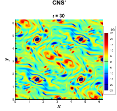
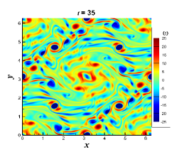
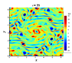
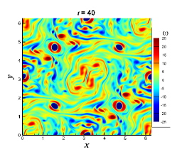
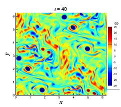
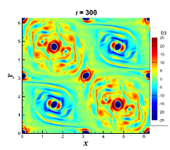
Figure 1: Comparisons of the vorticity field $\omega(x,y)$ of the 2D turbulent Kolmogorov flow governed by (1) and (2) in the case of $n_{K}=16$ and $Re=2000$ given by CNS, subject to either the initial conditions (3) (left, marked by CNS) or (9) (right, marked by CNS^′), respectively, at different times, i.e. (a)-(b): $t=30$; (c)-(d): $t=35$; (e)-(f): $t=40$; (g)-(h): $t=300$.

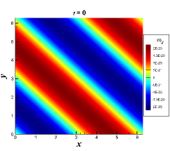
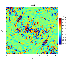
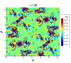
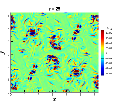
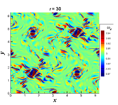
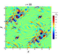
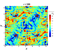
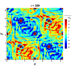
Figure 2: The vorticity field of the evolution $\delta_{1}(x,y,t)$ corresponding to the disturbance $10^{-20}\sin(x+y)$ of the initial condition (9) of the 2D turbulent Kolmogorov flow governed by (1) and (2) in the case of $n_{K}=16$ and $Re=2000$ given by CNS at the different times, i.e. (a) $t=0$, (b) $t=8$, (c) $t=15$, (d) $t=25$, (e) $t=30$, (f) $t=35$, (g) $t=100$, (h) $t=300$, respectively.

As shown in Fig. 1, the vorticity field $\omega(x,y,t)$ of the flow CNS, subject to the initial condition (3), is compared with that of the flow CNS^′, subject to the initial condition (9). Note that the CNS flow remains the spatial symmetry (7) of vorticity throughout the whole interval of time $t\in[0,300]$. Obviously, the term $10^{-20}\,\sin(x+y)$ in the initial condition (9) can be regarded as a micro-level disturbance added to the initial condition (3), since it is 20 orders of magnitude smaller. Certainly, it takes some time for this tiny disturbance $10^{-20}\,\sin(x+y)$ to be enlarged to a macro-level $O(1)$. Indeed, the CNS^′ flow looks like the same as the CNS flow from the beginning, for example at $t=30$ as shown in Fig. 1(a) and (b), when $\delta_{1}(x,y,t)$ corresponding to the tiny disturbance $10^{-20}\sin(x+y)$ of the initial condition (9) has not been increased to macro-level, as shown in Fig. 2 (a)-(e), so that both of the flow CNS and the flow CNS^′ agree well and remain the same spatial symmetry (7) of vorticity. It is found that the vorticity of the flow CNS^′ deviates from the spatial symmetry (7) obviously at $t\approx 35$ and thereafter loses the spatial symmetry (7) but remains the spatial symmetry (8) throughout the interval of time $t\in[35,300]$ instead, as shown in Fig. 1(c)-(h), respectively. Note that the term $\sin(x+y)$ of the initial condition (9) has the spatial symmetry of translation but no spatial symmetry of rotation since $\sin(x+y)=\sin(\pi+x+\pi+y)$ but $\sin(x+y)\neq\sin(2\pi-x+2\pi-y)$. So, the reason is very clear from Fig. 2: $\delta_{1}(x,y,t)$ corresponding to the disturbance $10^{-20}\,\sin(x+y)$ in the initial condition (9) increases from a micro-level, step by step, to a macro-level at $t\approx 35$, which remains the same spatial symmetry (8) throughout the whole time interval $t\in[0,300]$ so that it destroys the spatial symmetry (7) and triggers the transition of the spatial symmetry from (7) to (8) at $t\approx 35$ when it reaches a macro-level $O(1)$. This provides us a rigorous evidence that, the very small disturbance $10^{-20}\,\sin(x+y)$ of the initial condition (9) indeed increases to the same order of magnitude as the exact solution of the NS equations at $t\approx 35$, which destroys the spatial symmetry (7) and triggers the transition of the spatial symmetry from (7) to (8).

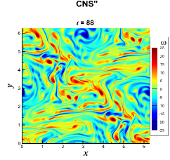
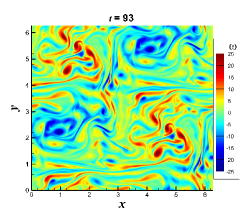
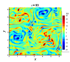
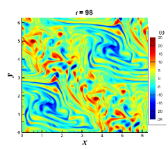
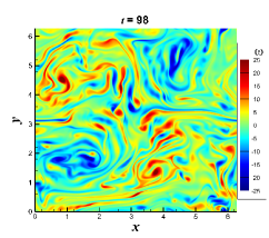
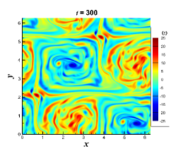
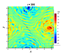
Figure 3: Comparisons of the vorticity fields $\omega(x,y)$ of the 2D turbulent Kolmogorov flow governed by (1) and (2) in the case of $n_{K}=16$ and $Re=2000$ given by CNS, subject to either the initial conditions (9) (left, marked by CNS^′) or (10) (right, marked by CNS^′′), respectively, at the different times, i.e. (a)-(b): $t=88$; (c)-(d): $t=93$; (e)-(f): $t=98$; (g)-(h): $t=300$.

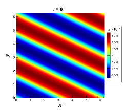
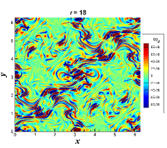
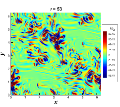
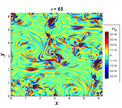
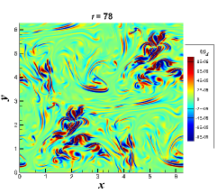
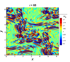
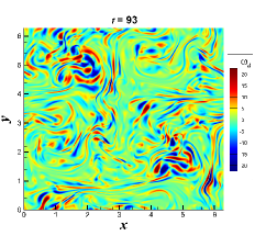
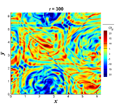
Figure 4: The vorticity field of the evolution $\delta_{2}(x,y,t)$ corresponding to the 2nd disturbance $10^{-40}\sin(x+2y)$ of the initial condition (10) of the 2D turbulent Kolmogorov flow governed by (1) and (2) in the case of $n_{K}=16$ and $Re=2000$ given by CNS at the different times, i.e. (a) $t=0$, (b) $t=18$, (c) $t=53$, (d) $t=65$, (e) $t=78$, (f) $t=88$, (g) $t=93$, (h) $t=300$, respectively.

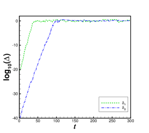
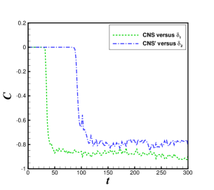
Figure 5: Time history of (a) $\Delta=\sqrt{\langle\delta_{i}^{2}\rangle}$, $i=1,2$, where $\delta_{1}(x,y,t)$ denotes the evolution of the 1st disturbance (green dashed line) and $\delta_{2}(x,y,t)$ is the evolution of the 2nd disturbance (blue dash-dotted line) of the initial condition (10), and (b) the normalized correlation coefficient $C(t)$ of vorticity of the flow CNS versus $\delta_{1}(x,y,t)$ (green dashed line), and that of the flow CNS^′ versus $\delta_{2}(x,y,t)$ (blue dash-dotted line) for the 2D turbulent Kolmogorov flow, governed by Eqs. (1) and (2) in the case of $n_{K}=16$ and $Re=2000$, subject to the initial condition (10).

As shown in Fig. 3, the vorticity field $\omega(x,y,t)$ of the flow CNS^′, subject to the initial condition (9), is compared with that of the flow CNS^′′, subject to the initial condition (10). Traditionally, compared with the 1st disturbance $10^{-20}\sin(x+y)$ in the initial condition (10), the 2nd disturbance $10^{-40}\sin(x+2y)$ could be neglected completely, since it is 20 orders of magnitude smaller. However, it is found that this traditional viewpoint is wrong in fact: the flow CNS^′′ looks like the same as the flow CNS from the beginning until $t\approx 35$ when it loses the spatial symmetry (7) but has the new spatial symmetry (8) instead, indicating that $\delta_{1}(x,y,t)$ corresponding to the 1st disturbance $10^{-20}\,\sin(x+y)$ increases to macro-level $O(1)$ and thus triggers the transition of the spatial symmetry from (7) to (8). More importantly, it is found that the flow CNS^′′ looks like the same as the flow CNS^′ from the beginning, for example at $t\approx 88$ as shown in Fig. 3 (a) and (b), until $t\approx 93$ when it loses the spatial symmetry (8), as shown in Fig. 3 (c) and (d). Note that the flow CNS^′′ completely loses the spatial symmetry after $t\geq 98$, as shown in Fig. 3 (e)-(h), clearly indicating that the evolution $\delta_{2}(x,y,t)$, corresponding to the 2nd micro-level disturbance $10^{-40}\sin(x+2y)$, must increase to a macro-level $O(1)$ and finally destroys the spatial symmetry at all. Note that the term $\sin(x+2y)$ has no spatial symmetry of rotation and translation, since $\sin(x+2y)\neq\sin(2\pi-x+4\pi-2y)$ and $\sin(x+2y)\neq\sin(\pi+x+2\pi+2y)$. So, the reason is very clear from Fig. 4: $\delta_{2}(x,y,t)$, corresponding to the 2nd disturbance $10^{-40}\,\sin(x+2y)$ in the initial condition (10), increases from a micro-level, step by step, to a macro-level at $t\approx 93$, which has no spatial symmetry at all throughout the whole time interval $t\in[0,300]$ so that it destroys the spatial symmetry (8) at $t\approx 93$ when it reaches a macro-level $O(1)$.

Let us focus on the initial condition (10): the 2nd disturbance $10^{-40}\,\sin(x+2y)$ is 20 orders of magnitude smaller than the 1st disturbance $10^{-20}\sin(x+y)$. From the traditional viewpoint, the 2nd disturbance should be negligible compared to the 1st one. However, on the contrary, both of the 1st disturbance $10^{-20}\,\sin(x+y)$ and the 2nd disturbance $10^{-40}\,\sin(x+2y)$ of the initial condition (10) enlarge separately, one by one like an inverse cascade, to macro-level $O(1)$: first the former triggers the transformation of the spatial symmetry from (7) to (8) at $t\approx 35$ and then the latter totally destroys the spatial symmetry of the 2D turbulent Kolmogorov flow at $t\approx 93$. This is very clear from Fig. 2 for the evolution $\delta_{1}(x,y,t)$ of the 1st disturbance $10^{-20}\sin(x+y)$ and Fig. 4 for the evolution $\delta_{2}(x,y,t)$ of the 2nd disturbance $10^{-40}\sin(x+2y)$ of the initial condition (10).

Note that, as shown in Fig. 2, the vorticity field caused by $\delta_{1}(x,y,t)$ corresponding to the 1st disturbance $10^{-20}\sin(x+y)$ increases from a micro-order $O(10^{-20})$ of magnitude at $t=0$, step by step, to the order $O(10^{-15})$ at $t=8$, $O(10^{-10})$ at $t=15$, $O(10^{-5})$ at $t=25$, $O(10^{-2})$ at $t=30$, until to a macro-order $O(10)$ at $t=35$, respectively. Similarly, as shown in Fig. 4, the vorticity field caused by $\delta_{2}(x,y,t)$ corresponding to the 2nd disturbance $10^{-40}\sin(x+2y)$ increases from a micro-order $O(10^{-40})$ of magnitude at $t=0$, step by step, to the order $O(10^{-30})$ at $t=18$, $O(10^{-15})$ at $t=53$, $O(10^{-10})$ at $t=65$, $O(10^{-5})$ at $t=78$, $O(10^{-1})$ at $t=88$, until to a macro-order $O(10)$ at $t=93$, respectively. All of these at different orders of magnitude often coexist with macroscopic flow field.

Write $\Delta=\sqrt{\langle\delta_{i}^{2}\rangle}$, $i=1,2$, where $\delta_{1}(x,y,t)$ denotes the evolution of the first disturbance $10^{-20}\sin(x+y)$ and $\delta_{2}(x,y,t)$ the evolution of the second disturbance $10^{-40}\sin(x+2y)$ in the initial condition (10), respectively, and $\langle\;\rangle$ is an operator of statistics defined in Appendix. As shown in Fig. 5 (a), $\sqrt{\langle\delta_{1}^{2}\rangle}$ exponentially expands until $t\approx 35$ when it reaches a macro-level. i.e. $\sqrt{\langle\delta_{1}^{2}\rangle}\sim O(1)$. Similarly, $\sqrt{\langle\delta_{2}^{2}\rangle}$ exponentially expands until $t\approx 93$ when it is at a macro-level. i.e. $\sqrt{\langle\delta_{2}^{2}\rangle}\sim O(1)$. As mentioned before, the flow CNS^′ is equal to the flow CNS plus $\delta_{1}(x,y,t)$, and the flow CNS^′′ is equal to the flow CNS^′ plus $\delta_{2}(x,y,t)$, respectively. As shown in Fig. 5 (b), the normalized correlation coefficient of vorticity of the flow CNS versus $\delta_{1}$ is very small from the beginning to $t\approx 32$, indicating no correlation between them at all because $\delta_{1}(x,y,t)$ is negligible compared to the flow CNS, until $t\approx 35$ when their correlation suddenly becomes strong, indicating that $\delta_{1}(x,y,t)$ is at the same order of magnitude as the flow CNS and thus is not negligible thereafter. Similarly, the normalized correlation coefficient of vorticity of the flow CNS^′ versus $\delta_{2}(x,y,t)$ is very small from the beginning to $t\approx 90$, indicating no correlation between them at all because $\delta_{2}(x,y,t)$ is negligible compared to the flow CNS^′, until $t\approx 93$ when their correlation suddenly becomes strong, indicating that $\delta_{2}(x,y,t)$ is at the same order of magnitude as the flow CNS^′ and thus is not negligible thereafter.

All of these provide us rigorous evidence that all disturbances at different orders of magnitudes of initial condition of the NS equations increase separately, say, one by one like an inverse cascade, to macro-level, and besides each of them could completely change the characteristics of the turbulent flow considered in this paper. Based on this very interesting phenomenon revealed by our “clean” numerical experiments mentioned above, we propose a new concept, namely “noise-expansion cascade”, which closely connects randomness of micro-level noises/disturbances and macro-level disorder of turbulence.

3.3 Influences of noise-expansion cascade on statistics

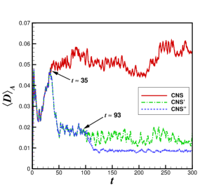
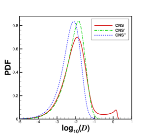
Figure 6: Comparisons of (a) time histories of the spatially averaged kinetic energy dissipation rate $\langle D\rangle_{A}$ and (b) the probability density function (PDF) of the kinetic energy dissipation $D(x,y,t)$ of the 2D turbulent Kolmogorov flow, governed by Eqs. (1) and (2) in the case of $n_{K}=16$ and $Re=2000$, given by the flow CNS subject to the initial condition (3) (solid line in red), the flow CNS^′ subject to the initial condition (9) (dash-dot line in green) and the flow CNS^′′ subject to the initial condition (10) (dashed line in blue), respectively.

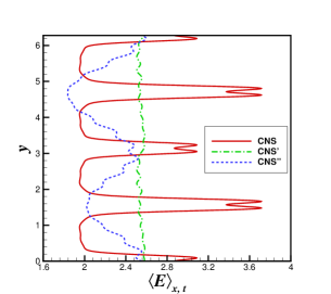
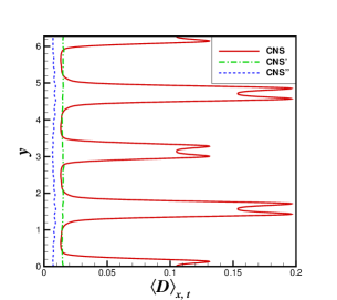
Figure 7: Comparisons of (a) the spatio-temporal averaged kinetic energy $\langle E\rangle_{x,t}(y)$ and (b) the spatio-temporal averaged kinetic energy dissipation rate $\langle D\rangle_{x,t}(y)$ of the 2D turbulent Kolmogorov flow, governed by Eqs. (1) and (2) in the case of $n_{K}=16$ and $Re=2000$, given by the flow CNS subject to the initial condition (3) (solid line in red), the flow CNS^′ subject to the initial condition (9) (dash-dot line in green) and the flow CNS^′′ subject to the initial condition (10) (dashed line in blue), respectively.

Fig. 6 (a) shows the comparisons of the time histories of the spatially averaged kinetic energy dissipation rate $\langle D\rangle_{A}$ of the flow CNS, the flow CNS^′ and the flow CNS^′′, respectively, where $\langle\;\rangle_{A}$ is an operator of statistics defined in Appendix. The distinct deviation of $\langle D\rangle_{A}$ between the flow CNS and the flow CNS^′ appears at $t\approx 35$ when the evolution $\delta_{1}(x,y,t)$ of the 1st disturbance $10^{-20}\sin(x+y)$ increases to a macro-level $O(1)$ that finally destroys the spatial symmetry (7) and triggers the transformation of the spatial symmetry from (7) to (8). Besides, the distinct deviation of $\langle D\rangle_{A}$ of the flow CNS^′ versus the flow CNS^′′ appears at $t\approx 93$ when the evolution $\delta_{2}(x,y,t)$ of the 2nd disturbance $10^{-40}\sin(x+2y)$ increases to a macro-level $O(1)$ that finally destroys the spatial symmetry at all. As shown in Fig. 6 (a), when $t>110$, the spatially averaged kinetic energy dissipation rate $\langle D\rangle_{A}$ of the flow CNS is much larger than those of the flow CNS^′ and the flow CNS^′′. This leads to the obvious deviation between their probability density function (PDF), as shown in Fig. 6 (b), respectively. Fig. 7 shows the comparisons of the spatio-temporal averaged kinetic energy $\langle E\rangle_{x,t}(y)$ and the spatio-temporal averaged kinetic energy dissipation rate $\langle D\rangle_{x,t}(y)$ of the flow CNS, the flow CNS^′ and the flow CNS^′′, respectively, where $\langle\;\rangle_{x,t}$ is an operator of statistics defined in Appendix. Note that these statistics have obvious deviations, too.

Thus, not only all disturbances at different orders of magnitudes of initial condition of the NS equations increase, one by one like an inverse cascade, to a macro-level, but also each of them could sometimes completely change macro-level characteristics of turbulent flow, even including some statistic properties, as illustrated above.

3.4 An origin of randomness of turbulence

The most surprising of the “noise-expansion cascade” phenomenon is the fact that all disturbances, even if they are at quite different orders of magnitude, separately enlarge to macro-level, one by one like an inverse cascade. For example, for the CNS^′′ flow subject to the initial condition (10), the evolution $\delta_{1}(x,y,t)$ of the first disturbance $10^{-20}\sin(x+y)$ increases to macro-level at $t\approx 35$ and then triggers the transformation of the spatial symmetry of the flow field from (7) to (8), but the evolution $\delta_{2}(x,y,t)$ of the 2nd disturbance $10^{-40}\sin(x+2y)$ totally destroys the spatial symmetry of the turbulent flow at all when it increases to macro-level at $t\approx 93$. This clearly indicates that the 2nd disturbance $10^{-40}\sin(x+2y)$ of the initial condition (10) can lead to great change to characteristics of the turbulence, although it is 20 orders of magnitude smaller than the 1st ones. This highly suggests that all disturbances must be considered for turbulence. This answers our 2nd open question mentioned at the beginning of this paper.

Note that internal thermal fluctuation and external environmental disturbance are unavoidable in practice. In general, environmental disturbance is much larger than thermal fluctuation. So, traditionally, thermal fluctuation is neglected for most of turbulent flows, especially those governed by NS equations. However, according to the new concept “noise-expansion cascade”, thermal fluctuation must be considered for turbulence, even if it is many orders of magnitude smaller than environmental disturbance. Note that thermal fluctuation is random in essence, and such kind of randomness can naturally transfer from micro-level to macro-level through the “noise-expansion cascade”. Therefore, the “noise-expansion cascade” reveals an origin of randomness of turbulence. This answers our 1st open question mentioned at the beginning of this paper.

4 Conclusion and discussion

It was found [15, 16] that spatiotemporal trajectory given by “direct numerical simulation” (DNS) is quickly polluted by artificial numerical noise badly so that it is impossible to use DNS to accurately and rigorously simulate the evolution and propagation of small disturbances in turbulent flow. Fortunately, “clean numerical simulation” (CNS) [10, 11, 12, 13] has much smaller artificial numerical noise than DNS and thus provides us the ability to do “clean” numerical experiments for turbulence. In this paper, by means of several ingeniously designed clean numerical experiments based on CNS for a 2D turbulent Kolmogorov flow, it is discovered, for the first time, that all disturbances at different orders of magnitude in initial condition of NS equations quickly enlarge separately, one by one like an inverse cascade, to macro-level, and besides each of them might greatly change characteristics of the turbulent flow not only in the spatial symmetry of the flow but also even in the statistics, as illustrated in this paper. Based on this interesting phenomenon, a new concept, namely “noise-expansion cascade”, is proposed. The so-called “noise-expansion cascade” closely connects randomness of micro-level noise/disturbance and macro-level disorder of turbulence, and thus reveals an origin of randomness of turbulence. This answers our 1st open question mentioned at the beginning of this paper. It should be emphasized that the “noise-expansion cascade” as a new fundamental concept of turbulence cannot be discovered by numerical experiment based on DNS or in a physical laboratory: this illustrates the great potential of CNS.

Note that internal thermal fluctuation and external environmental disturbance are unavoidable in practice. So, according to the “noise-expansion cascade”, thermal fluctuation should be considered for turbulence, even if it is much smaller than external environmental disturbance, just like the Landau-Lifshitz-Navier-Stokes equations that includes the influence of thermal fluctuation[26]. This answers the 2nd open question that we mentioned at the beginning of this paper. Note that the influence of thermal fluctuation on turbulence has been reported currently by few researchers [27, 28].

Due to the “noise-expansion cascade”, many micro-level random factors might have great influences on macro-level disorder of turbulence: the “noise-expansion cascade” should be a bridge connecting micro-level random fluctuation/disturbance and macro-level disorder of turbulence. So, the “noise-expansion cascade” as a new concept might provide us a scientific reason why “people cannot step twice into the same river”, which was pointed out by philosopher Heraclitus. It highly suggests that turbulence should be a kind of unity of micro-level random noise/disturbance, their evolution and propagation, and macro-level disorder, which are closely connected through the “noise-expansion cascade”: this can well explain why turbulence is so difficult to understand.

Note that the “noise-expansion cascade” has obvious difference from “energy cascade”, a fundamental concept in turbulence theory. There are two types of energy cascade, say, direct energy cascade with energy transfer from large scale to small scale, and inverse energy cascade with energy transfer from small scale to large scale. However, unlike energy cascade, noise-expansion cascade has only one direction: from micro-scale to large scale. Besides, energy cascade describes spatial transfer of energy, but noise-expansion cascade describes temporal evolution and propagation of disturbances. This also indicates the novelty of noise-expansion cascade as a new fundamental concept of turbulence.

At each time-step, DNS algorithm unavoidably contains artificial numerical noise. Thus, due to noise-expansion cascade, the artificial numerical noise of DNS algorithm at each time-step should increase consistently to macro-level: this is exactly the reason why spatiotemporal trajectory of DNS departs quickly from true solution. This is the reason why noise-expansion cascade cannot be discovered by DNS.

There are many interesting problems worthy of further investigation in future. For example, it might be possible that artificial numerical noise could be regarded as a kind of physical external disturbance, as long as we could prove that artificial numerical noise could have same influences as thermal fluctuation and/or environmental disturbance to turbulent flow, which unfortunately is still an open question until now. This kind of investigations might reveal the essence of artificial numerical noises to turbulent flow. Besides, thermal fluctuation is random and discontinuous, but it is still an open question whether or not such random and discontinuous disturbance might become continuous when it increases to macro-level due to noise-expansion cascade.

Indeed CNS is time-consuming today, just like DNS in 1970 when Orszag [3] proposed it. For the 2D turbulent Kolmogorov flow under consideration, the parallel computing of the CNS takes 285 hours (i.e. about 12 days) using 4096 CPUs (Intel’s CPU: Xeon Gold 6348, 2.60GHz) of “Tian-He New Generation Supercomputer” at National Supercomputer Center in Tianjin, China. By contrast, the DNS for the same case needs only 13 hours using 1024 CPUs at the same computing platform. Even so, without doubt, CNS could provide us a new strategy to investigate turbulence by doing clean numerical experiments, i.e. with rigorously negligible artificial numerical noise, which should allow a better understanding of the physics of turbulence.

Finally, we would like to emphasize that DNS is a milestone in fluid mechanics, since it opened a new times of numerical experiment and has greatly promoted the progress of turbulence in theories, physical experiments and applications. In essence, CNS can be regarded as a general DNS with rigorously negligible numerical noises in a finite but long enough interval of time, which is powerful and helpful to accurately investigate influence of micro-scale physical/artificial disturbances on turbulent flow.

Appendix
Some definitions and measures

For the sake of simplicity, the definitions of some statistic operators are briefly described below. The operator of spatial average is defined by

$$\langle\,f\,\rangle_{A}=\frac{1}{4\pi^{2}}\int^{2\pi}_{0}\int^{2\pi}_{0}f\,dxdy,$$ (S1)

the operator of spatiotemporal average (along the $x$ direction) is defined by

$$\langle\,f\,\rangle_{x,t}=\frac{1}{2\pi(T_{2}-T_{1})}\int^{2\pi}_{0}\int^{T_{2}}_{T_{1}}f\,dxdt,$$ (S2)

and the operator of spatiotemporal average (over the whole field) is defined by

$$\langle\,f\,\rangle=\frac{1}{4\pi^{2}(T_{2}-T_{1})}\int^{2\pi}_{0}\int^{2\pi}_{0}\int^{T_{2}}_{T_{1}}f\,dxdydt,$$ (S3)

respectively, where $T_{1}=100$ (for the flow CNS and the flow CNS^′) or $120$ (for the flow CNS^′′) and $T_{2}=300$ are used in this paper to calculate statistics.

The kinetic energy is given by

$$E(x,y,t)=\frac{1}{2}\Big{[}u^{2}(x,y,t)+v^{2}(x,y,t)\Big{]}$$ (S4)

and the kinetic energy dissipation rate is defined by

$$D(x,y,t)=\frac{1}{2Re}\sum_{i,j=1,2}\Big{[}\partial_{i}u_{j}(x,y,t)+\partial_{j}u_{i}(x,y,t)\Big{]}^{2},$$ (S5)

respectively, where $u_{1}(x,y,t)=u(x,y,t)$, $u_{2}(x,y,t)=v(x,y,t)$, $\partial_{1}=\partial/\partial x$, and $\partial_{2}=\partial/\partial y$.

Acknowledgements

The calculations were performed on “Tian-He New Generation Supercomputer”, National Supercomputer Center in Tianjing, China. This work is partly supported by National Natural Science Foundation of China (Grant No. 12272230 and 91752104), Postdoctoral Fellowship Program of CPSF (Grant No. GZC20231594), and State Key Laboratory of Ocean Engineering.

References

- [1] P. A. Davidson, Turbulence : an introduction for scientists and engineers, Oxford University Press, Oxford, 2004.
- [2] Clay Mathematics Institute of Cambridge, The Millennium Prize Problems, https://www.claymath.org/millennium-problems/ (2000).
- [3] S. A. Orszag, Analytical theories of turbulence, J. Fluid Mech. 41 (2) (1970) 363 – 386.
- [4] R. S. Rogallo, Numerical experiments in homogeneous turbulence, Tech. Rep. NASA-TM-81315, NASA, USA (September 1981).
- [5] Z.-S. She, E. Jackson, S. A. Orszag, Intermittent vortex structures in homogeneous isotropic turbulence, Nature 344 (1990) 226 – 228.
- [6] M. Nelkin, In what sense is turbulence an unsolved problem?, Science 255 (1992) 566–570.
- [7] A. Alexakis, R. Marino, P. D. Mininni, A. van Kan, R. Foldes, F. Feraco, Large-scale self-organization in dry turbulent atmospheres, Science 383 (2024) 1005–1009.
- [8] G. N. Coleman, R. D. Sandberg, A primer on direct numerical simulation of turbulence –methods, procedures and guidelines, Tech. Rep. AFM-09/01a, Aerodynamics & Flight Mechanics Research Group, University of Southampton, UK (March 2010).
- [9] S. Liao, On the reliability of computed chaotic solutions of non-linear differential equations, Tellus Ser. A-Dyn. Meteorol. Oceanol. 61 (4) (2009) 550–564.
- [10] S. Liao, Clean Numerical Simulation, Chapman and Hall/CRC, 2023.
- [11] T. Hu, S. Liao, On the risks of using double precision in numerical simulations of spatio-temporal chaos, J. Comput. Phys. 418 (2020) 109629.
- [12] S. Qin, S. Liao, Influence of numerical noises on computer-generated simulation of spatio-temporal chaos, Chaos Solitons Fractals 136 (2020) 109790.
- [13] S. Qin, S. Liao, A self-adaptive algorithm of the clean numerical simulation (CNS) for chaos, Adv. Appl. Math. Mech. 15 (5) (2023) 1191–1215.
- [14] P. Oyanarte, MP-a multiple precision package, Comput. Phys. Commun. 59 (2) (1990) 345–358.
- [15] S. Qin, S. Liao, Large-scale influence of numerical noises as artificial stochastic disturbances on a sustained turbulence, J. Fluid Mech. 948 (2022) A7.
- [16] S. Qin, Y. Yang, Y. Huang, X. Mei, L. Wang, S. Liao, Is a direct numerical simulation (DNS) of Navier-Stokes equations with small enough grid spacing and time-step definitely reliable/correct?, Journal of Ocean Engineering and Science 9 (2024) 293 – 310.
- [17] X. Li, S. Liao, More than six hundred new families of Newtonian periodic planar collisionless three-body orbits, Sci. China-Phys. Mech. Astron. 60 (12) (2017) 129511.
- [18] X. Li, Y. Jing, S. Liao, Over a thousand new periodic orbits of a planar three-body system with unequal masses, Publ. Astron. Soc. Jpn. 70 (4) (2018) 64.
- [19] S. Liao, X. Li, Y. Yang, Three-body problem – from Newton to supercomputer plus machine learning, New Astronomy 96 (2022) 101850.
- [20] L. Crane, Infamous three-body problem has over a thousand new solutions, New Scientist (20 September 2017).
- [21] C. Whyte, Watch the weird new solutions to the baffling three-body problem, New Scientist (25 May 2018).
- [22] A. M. Obukhov, Kolmogorov flow and laboratory simulation of it, Russian Math. Surveys 38 (4) (1983) 113–126.
- [23] G. J. Chandler, R. R. Kerswell, Invariant recurrent solutions embedded in a turbulent two-dimensional Kolmogorov flow, J. Fluid Mech. 722 (2013) 554–595.
- [24] W. Wu, F. G. Schmitt, E. Calzavarini, L. Wang, A quadratic Reynolds stress development for the turbulent Kolmogorov flow, Phys. Fluids 33 (2021) 125129.
- [25] S. B. Pope, Turbulent Flows, IOP Publishing, 2001.
- [26] L. D. Landau, E. M. Lifshitz, Course of Theoretical Physics: Fluid Mechanics (Vol. 6), Addision-Wesley, Reading, 1959.
- [27] D. Bandak, N. Goldenfeld, A. A. Mailybaev, G. Eyink, Dissipation-range fluid turbulence and thermal noise, Phys. Rev. E 105 (2022) 065113.
- [28] Q. Ma, C. Yang, S. Chen, K. Feng, Z. Cui, J. Zhang, Effect of thermal fluctuations on spectra and predictability in compressible decaying isotropic turbulence, J. Fluid Mech. 987 (2024) A29.