X-Shooting ULLYSES: Massive Stars at low metallicity IX:
Empirical constraints on mass-loss rates and clumping parameters for OB supergiants in the Large Magellanic Cloud

Abstract

Context. Current implementations of mass loss for hot, massive stars in stellar evolution models usually include a sharp increase in mass loss when blue supergiants become cooler than $T_{\rm eff}\sim 20-22$ kK. Such a drastic mass-loss jump has traditionally been motivated by the potential presence of a so-called bistability ionisation effect, which may occur for line-driven winds in this temperature region due to recombination of important line-driving ions.

Aims. We perform quantitative spectroscopy using UV (ULLYSES program) and optical (XShootU collaboration) data for 17 OB-supergiant stars in the Large Magellanic Cloud (LMC) (covering the range $T_{\rm eff}$ $\sim 14-32$ kK), deriving absolute constraints on global stellar, wind, and clumping parameters. We examine whether there are any empirical signs of a mass loss jump in the investigated region, and we study the clumped nature of the wind.

Methods. We use a combination of the model atmosphere code fastwind and the genetic algorithm (GA) code Kiwi-GA to fit synthetic spectra of a multitude of diagnostic spectral lines in the optical and ultra-violet (UV).

Results. We find an almost monotonic decrease of mass loss-rate with effective temperature, with no signs of any upward mass loss jump anywhere in the examined region. Standard theoretical comparison models, which include a strong bistability jump thus severely over predict the empirical mass-loss rates on the cool side of the predicted jump. Another key result is that across our sample we find that on average about 40% of the total wind mass seems to reside in the more diluted medium in between dense clumps.

Conclusions. Our derived mass-loss rates suggest that for applications like stellar evolution one should not include a drastic bistability jump in mass loss for stars in the temperature and luminosity region investigated here. The derived high values of interclump density further suggest that the common assumption of an effectively void interclump medium (applied in the vast majority of spectroscopic studies of hot star winds) is not generally valid in this parameter regime.

1 Introduction

An important process in the life of massive stars are stellar winds driven by radiation intercepted by a multitude of atmospheric spectral lines (Castor et al. 1975) that over time may cause the star to lose a sizeable fraction of their initial mass and angular momentum. This significantly influences the evolution of a massive stars, and, ultimately, the nature and characteristics of its end of life products (e.g., Heger et al. 2003; Langer 2012).

While studying luminous B-stars that experience such line-driven winds, Pauldrach & Puls (1990) and Lamers et al. (1995) noticed a peculiar behaviour in the ratio of terminal wind speed $\varv_{\infty}$ over surface escape speed $\varv_{\rm esc}$ which seemed to decrease sharply (by a factor of about two) for stars with an effective temperature ($T_{\rm eff}$) cooler than $\sim 21$ kK. Although these early results already hinted at the possibility of a corresponding increase in $\dot{M}$, such an increase was quantified by Vink et al. (1999, 2001). These authors, possibly, identified a recombination of iron (from Fe iv to Fe iii) near the sonic point. The increase in the amount of line transitions for Fe iii resulted in more efficient line-driving, as the underlying physical reason for the mass-loss jump. Based on these models, Vink et al. (2001) provide fit-formulae and corresponding ”mass-loss recipes” that are divided in a ”hot” and ”cool” prescription, where the exact location of the ”bistability” divide depends on metallicity $Z$ and the classical Eddington parameter ($\Gamma_{\rm e}$, see equation 8). Depending on these parameters, the cool solution in this recipe may have up to an order of magnitude more mass loss than the hot, resulting in big mass-loss jump, typically located somewhere in the range $T_{\rm eff}\sim 22.5-27.5$ kK. This prescription has meanwhile become a standard choice to describe mass-loss from line-driven winds in stellar evolution codes such as Modules for Experiments in Stellar Astrophysics (MESA) (Paxton et al. 2010, 2013, 2015) and the Geneva stellar evolution code genec (e.g., Groh et al. 2019). Studies of the effects of such a bistability mass loss jump in evolution calculations suggest that if this occurs during the final parts of the main sequence (or during post-main sequence evolution of stars that do not reach the red supergiant stage) substantial mass and angular momentum loss may occur. This then more easily allows for the formation of Wolf-Rayet stars (Björklund et al. 2023) and also causes bistability braking, i.e., a strong reduction of surface rotation speed at $T_{\rm eff}$ cooler than $\sim$ 21 kK (Vink et al. 2010; Keszthelyi et al. 2017; Britavskiy et al. 2024).

Considerable effort has been invested to understand the physical nature and effects of terminal velocity and mass-loss bi-stability. The Vink et al. (2000) models parametrise the wind velocity law $\varv(r)$, apply the Sobolev (1960) approximation for line transfer, constrain $\dot{M}$ from a global energy balance argument, and employ a modified nebular approximation to compute the state of the gas. In follow-up work, Müller & Vink (2008) and Muijres et al. (2012) used their computed Monte-Carlo line force to fit a parametrised radial function. By means of this function then, the equation of motion can be solved in an iterative manner until $\dot{M}$ and $\varv_{\infty}$ are converged. Vink (2018) applied this technique to luminous stars of different $T_{\rm eff}$ and found sharply decreasing $\varv_{\infty}$ accompanied by mass-loss rates that increased by more than an order of magnitude when decreasing $T_{\rm eff}$ from 25 to 18 kK (while keeping metallicity, luminosity, and mass fixed, see their Fig. 1). More recently, steady-state line-driven wind models that are based on co-moving frame (CMF) radiative transfer have been calculated (Krtička & Kubát 2017; Sander et al. 2017; Sundqvist et al. 2019; Björklund et al. 2021, 2023; Krtička et al. 2024). These simulations solve the equation of motion without parametrisation, and keep momentum conserved locally throughout the atmosphere and wind. Specifically, because of the difficulty of driving wind material through the critical sonic point the models computed by Björklund et al. (2023) for the B-star regime do not show any upward increase in mass-loss rate with decreasing $T_{\rm eff}$ (again keeping the metallicity and stellar luminosity to mass ratio fixed). The models by Krtička et al. (2024) do find a localised and small mass-loss increase (followed by a sharp decrease), but at significantly lower $T_{\rm eff}$ than 21 kK (see also Petrov et al. 2016). These calculations are also based on CMF radiative transfer and solve the full steady-state equation of motion. However, they scale their radiative accelerations to corresponding calculations based on the Sobolev approximation causing their critical point to shift from the sonic point to the point in the supersonic wind where the radiative-acoustic wave (known as an ’Abbott wave’, Abbott 1980) speed equals the flow velocity. Additionally, they compute bound-bound rates in the statistical equilibrium equations using this Sobolev approximation, neglecting velocity curvature effects in near-sonic regions (Owocki & Puls 1999) These may be potential causes for the differences in $\dot{M}$-behaviour seen between the (at first glance very similar) models by Krtička et al. (2024) and Björklund et al. (2023). Mass-loss rates from the three approaches outlined above are shown in Fig. 1, illustrating the significant differences in predicted rates for the region under study here. We point out that what is shown are fit-formulae to the underlying model-sets that not always capture the full $\dot{M}$ behaviour, introducing additional differences. For instance, in the case of the Vink et al. (2000) rates these formulae often enhance the size of the jump (which in the underlying model-set typically is about a factor of 5, Vink et al. 1999) through enforcing a discontinuous mass-loss jump.

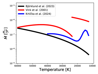
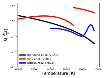
Figure 1: Comparison of mass-loss rates from prescriptions by Vink et al. (2001); Björklund et al. (2023); Krtička et al. (2024) over the temperature range from $60-12.5$ kK. Key stellar parameters in the left panel are: $\log_{10}(L_{\star}/L_{\odot})=5.3$, $M_{\star}=\,25M_{\odot}$ and, $Z=0.5\,Z_{\odot}$. This results in $\Gamma_{\rm e}=0.21$. In the right panel adopted properties are $\log_{10}(L_{\star}/L_{\odot})=5.6$, $M_{\star}=25\,M_{\odot}$ and, $Z=0.5\,Z_{\odot}$, yielding $\Gamma_{\rm e}=0.42$. The full lines signify that the result of the fit-formulate given by these authors are shown rather than the actual underlying model-sets. For the Vink et al. rates, for which a mass-loss jump is identified to cover the regime $\sim 22.5-27.5$ kK, enforcing a strict discontinuity (i.e. at a single temperature) implies that the size of the $\dot{M}$-jump is somewhat enhanced as compared to the underlying models.

So far, observational evidence of a bistability mass-loss jump has proven difficult to obtain. Trundle et al. (2004) comment that in their sample of small Magellanic cloud (SMC) B-(super)giants, for which they obtained optical spectra, the mass-loss rates of stars at the cool side of the jump are noticeably smaller than the Vink et al. (2001) prescription. Additionally, Markova & Puls (2008) do not find a jump from an optical H ${\alpha}$ analysis of B-supergiants (BSGs) and neither do Rubio-Díez et al. (2022), studying continuum infra-red and radio data of bright OB-stars. Most recently a large scale study on 116 B-supergiants in the Galaxy, based on optical spectra only, found no evidence for a bistability jump (de Burgos et al. 2024). Benaglia et al. (2007), however, do claim tentative signs of a mass-loss increase for stars cooler than $T_{\rm eff}\sim 21$ kK in their radio analysis. A common denominator of these studies is that they rely solely on diagnostic features for which the associated opacities depend on the square of the density. This makes these mass-loss constraints prone to degeneracies introduced by wind inhomogeneities (or ‘clumping’, see, e.g., Puls et al. 2008). By combining spectroscopy in the optical and ultra-violet (UV) (see also Bernini-Peron et al. 2023), we here aim to break these degeneracies and derive absolute constraints on mass-loss rates as well as wind clumping properties.

With the completion of the data taking in the Hubble UV Legacy Library of Young Stars as Essential Standards (ULLYSES) (Roman-Duval et al. 2020) and XShooting ULLYSES (XShootU) (Vink et al. 2023; Sana et al. 2024) programs we now a have a unique UV and optical data set of late-O and early- and mid-B type in the Large Magellanic Cloud (LMC). This allows us to, for the first time, constrain stellar, mass-loss and wind-clumping characteristics across the anticipated bistability region for a statistically relevant sample. Hence it also permits for the most direct confrontation of empirical results to predictions of mass loss and clumping (Driessen et al. 2019) in the $14-33$ kK blue supergiant regime to date. To fit these new data we utilise a combination of fastwind (v10.5, Puls et al. 2005; Sundqvist & Puls 2018) and Kiwi-GA (Brands et al. 2022). Previous empirical studies utilising this method for spectroscopic analysis include Hawcroft et al. (2021); Brands et al. (2022); Hawcroft et al. (2024a); Backs et al. (2024) Brands et al. (in prep.). From here on, we will refer to Hawcroft et al. (2021) as H21 and Brands et al. (2022) as B22.

We first present the dataset utilised to conduct our investigation in Sect. 2.1 and introduce fastwind (Sect. 2.2) and Kiwi-GA (Sect. 2.3). In Sect. 3, we describe the stellar, wind, and clumping parameters obtained from fitting the data, with special attention to mass-loss rates and clumping properties. In Sect. 4, we first discuss the influence of some of the choices made during the fitting process, after which we examine the results. Our main findings are that mass-loss does not seem to ’jump’ across the bi-stability jump, nor do the clumping properties (which have sizeable uncertainties) show a discontinuous behaviour. We do find a similar downward trend in terminal wind speeds with effective temperature as has been reported previously, though the scatter in especially the ratio $\varv_{\infty}/\varv_{\rm esc}$ is large for our sample. We also find that, on average, about 40 % of the total wind mass seems not to reside in dense clumps, bur rather in the more diluted medium around them. Implications of these results to the wider field are discussed.

2 Observations and methodology

In this section we describe our chosen sample of LMC OB-supergiants (BSGs), the stellar atmosphere and spectral synthesis code fastwind used to model the stars in our sample, and the genetic-algorithm (GA) code, Kiwi-GA, used to determine the optimum parameter values and their uncertainties.

2.1 Dataset

We selected 15 B-supergiant stars and two late O I-III stars in the LMC from the Hubble Space Telescope legacy program ULLYSES (Roman-Duval et al. 2020) in which UV spectra for   250 sources in the Magellanic Clouds are taken with the Space Telescope Imaging Spectrograph (STIS) and Cosmic Origins Spectrograph (COS) spectrographs. This program is complemented by the Very Large Telescope (VLT)/X-shooter large program XshootU (Vink et al. 2023; Sana et al. 2024) that collects optical spectra of the same sources. Our dataset covers the spectral range B7 through O8.5, which roughly corresponds to temperatures from 14 kK to 33 kK, i.e., the range in which the bistability jump in mass loss is predicted and the terminal wind velocity divided by the escape speed has been seen to change by about a factor two (Lamers et al. 1995). The reduced STIS spectra used are from ULLYSES data release DR6; the X-shooter spectra are from XShootU DR2. The photometric K-band data used for absolute calibration of the spectra is from Vink et al. (2023). Star identifications, spectral type and K-band photometry are given in Table 1. The Hubble space telescope (HST)/COS has multiple gratings, the G130M/1096 grating has a spectral resolving power of $\leavevmode\nobreak\ 6000$ ranging from $940-1240\AA$. The G130M/1291 and the G160M grating have a resolving power ranging from 11000 to 19000 and cover the wavelength range from $1141-1783\AA$. The HST/STIS spectra obtained using the E140M and the E230M grating cover a range of $1141-1708\AA$ and $1608-2366\AA$ respectively. The resolving power of the E140M grating is 48500, and the E230M grating has a resolving power of 30000. If multiple data sets would cover a modelled feature, the used data was chosen based on signal-to-noise ratio and resolving power. The optical data has two sections, the VIS and the UVB arm from VLT/X-shooter which have been stitched together by Sana et al. (2024). The UVB arm covers a spectral range from $3100-5500\AA$ with a spectral resolving power of 6700 for the chosen slit width of $0.8"$. The VIS arm covers the longer wavelengths from $5500\AA$ to $8000\AA$ and has a resolving power of 11400 for the slit width of $0.7"$. The visual spectra have a high S/N which is usually higher than 100. The UV data has a lower S/N at around 20.

Table 1: Full sample of stars used in this paper.

Star name	Revised SpT	SpT	$K_{s}$ (mag)	UV-observation
Sk$-67^{\circ}195$	B7 Ib	B6 I	12.68	E230M; G130M; G160M; G185M; G430L
Sk$-68^{\circ}8$		B5 Ia+	11.16	E230M; G130M; G160M; G430L
RMC-109		B5 Ia	12.09	E230M; G130M; G160M
Sk$-67^{\circ}78$		B3 Ia	11.35	E230M; FUSE; G130M; G160M
Sk$-70^{\circ}50$		B3 Ia	11.22	E230M; FUSE; G130M; G160M
Sk$-68^{\circ}26$		B2 Ia	11.27	E230M; FUSE; G130M; G160M; G230LB; G430L
Sk$-70^{\circ}16$	B2 II	B4 I	13.34	G130M; G160M; G185M; G430L
Sk$-69^{\circ}52$		B2 Ia	11.58	E230M; FUSE; G130M; G160M
Sk$-67^{\circ}14$	B1 Ia	B1.5 Ia	11.90	E140M; E230M; FUSE
Sk$-69^{\circ}140$	B1 Ib	B4 I	13.07	E230M; G130M; G160M
Sk$-66^{\circ}35$	BC1 Iab	BC1 Ia	11.69	E140M; E230M; FUSE
Sk$-69^{\circ}43$	B0.7 Ia	B0.5 Ia	12.15	E140M; E230M; FUSE
Sk$-68^{\circ}41$	B0.7 Ia	B0.5 Ia	12.24	E140M; E230M; FUSE
Sk$-68^{\circ}52$		B0 Ia	11.72	E140M; E230M; FUSE
Sk$-68^{\circ}155$	O9 Ia	B0.5 Ia	12.6	E230M; FUSE G130M; G160M
Sk$-67^{\circ}107$	O8.5 II	O9 Ib	13.06	E140M; FUSE
Sk$-67^{\circ}106$	O8 II	O8 III	12.39	E140M; FUSE; G230LB; G430L

• Notes: The spectral type and photometry is taken from Vink et al. (2023). We also include revised spectral types based on the XShootu data set from Crowther (in prep.). All objects have been observed using STIS. Here we show which grating was used and whether it was also observed using Far Ultraviolet Spectroscopic Explorer (FUSE).

2.2 fastwind

The unified model atmosphere code fastwind solves the NLTE rate equations assuming statistical equilibrium in a spherically symmetric and stationary extended stellar envelope comprising both the photosphere and the outflowing wind. We employ here version 10.5 (see Puls et al. 2005; Rivero González et al. 2012; Sundqvist & Puls 2018; Carneiro et al. 2018), which accounts for the accumulative feedback-effects from the multitudes of metallic spectral lines upon the radiation field and atmospheric structure by means of a computationally efficient statistical method. Some of those chemical elements, that are subsequently used for detailed spectroscopy (here H, He, Si, C, N, O), are treated separately using more precise radiative transfer calculations (for details, Puls et al. 2005).

The atmospheric structure is computed assuming (quasi-)hydrostatic equilibrium in the deeper atmospheric layers, connecting smoothly to an analytic wind outflow with radial velocity field $\varv(r)=\varv_{\infty}(1-bR_{\ast}/r)^{\beta}$ and average density structure $\langle\rho(r)\rangle=\dot{M}/(4\pi\varv(r)r^{2})$. The transition between the (quasi-)hydrostatic atmosphere and the wind is set to occur at a velocity $0.1$ times the gas sound speed at effective temperature. Here the input parameters describing the wind are the mass-loss rate $\dot{M}$, wind acceleration parameter $\beta$, and terminal wind speed $\varv_{\infty}$. $bR_{\ast}$ is the radius at the photospheric boundary. These parameters supplement the effective temperature $T_{\rm eff}$, surface gravity $g$, stellar radius $R_{\ast}$, and atmospheric chemical abundances in the list of input stellar and wind parameters describing the model atmosphere. Regarding elemental abundances we here adopt the solar composition by Asplund et al. (2009), and scale the overall metallic abundances ($Z$) accordingly to 0.5 times solar composition to match the LMC. The helium to hydrogen number abundance ratio, $Y_{\rm He}$, as well as some specific metal abundances (carbon, nitrogen, oxygen), are free-parameters in the fitting procedure. The silicon abundance is set to 7.2 dex (defined as $\log_{10}\epsilon_{\rm Si}=log(N_{\rm Si}/N_{H}+12$) as in Brott et al. (2011) (differing slightly from the value given in Vink et al. 2023) and is not used as a fit parameter. This constant Si-abundance has been chosen as we expect the Si-abundance to be nearly constant over the LMC. Additionally, the GA methodology used here is not optimised to constrain abundances as these will only have a small effect on the overall goodness of fit. We re-fitted several of the targets spread over the temperature range to determine if including the Si-abundance (and micro-turbulence, see below) as a free parameter changes the results of the other parameters. All fits of the test stars had a large uncertainty margin for the Si-abundance which enveloped our baseline of 7.2 dex. This suggests that our choice of not including the Si-abundance as a fit-parameter has not influenced our other results. Additionally, the new best fit Si-abundance was within 0.2 dex of the assumed value.

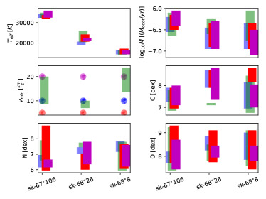
Figure 19: Results of the micro-turbulence variation tests. We show for three stars, four different fits. These 4 fits are very similar except for the photospheric micro turbulence, which is changed from a fixed 10 km/s we used in the paper (blue), to 5 km/s (red), to 20 km/s (purple), and left as a fit parameter (green). We plot the 1-$\sigma$ uncertainty of 5 parameters besides the $\varv_{\rm mic}$. These are: effective temperature, mass loss rate, and the CNO abundance. The three different stars each get a column in the 6 different panels and the 4 different fits are slightly overlapping in this column.

Inhomogeneities in the wind are described with the effective opacity formalism from Sundqvist & Puls (2018), incorporating modifications in opacity associated with clumping in physical and velocity-space. This formalism assumes a stochastic two-component wind consisting of over-dense clumps and a rarefied interclump medium. Mean densities are related to the root-mean-square (rms) average via a clumping factor $f_{\rm cl}\equiv\langle\rho^{2}\rangle/\langle\rho\rangle^{2}\geq 1$ and the interclump densities $\rho_{\rm ic}$ set by $f_{\rm ic}\equiv\rho_{\rm ic}/\langle\rho\rangle\geq 0$. Light-leakage effects in spectral lines (’velocity-porosity’) are accounted for by a velocity filling factor $0\leq f_{\rm vel}\leq 1$, defined as the fraction of the velocity field covered by the dense clumps. Wind clumping is assumed to start at some wind velocity $\varv_{\rm cl,start}>a$, where $a$ is the gas sound speed, and then increase linearly with velocity until the input parameter-values for $f_{\rm cl}$, $f_{\rm ic}$, and $f_{\rm vel}$ are reached at $\varv_{\rm cl,max}$. Clump optical depths for spectral lines are calculated from the input parameters using the Sobolev (1960) approximation; that is, we do not assume that clumps are optically thin or thick but instead compute them for all lines according to the structure parameters, to evaluate corresponding effects upon the ionisation balance and spectrum formation. The ionisation balance is then calculated for an average effective medium taking into account the clumped and interclumped components. Moreover, the micro-turbulent velocity is assumed to increase linearly with wind velocity from a fixed photospheric value $\varv_{\rm mic}=10$ km/s to a maximum value set by an input parameter scaled to the terminal wind speed. To quantify the effects of fixing the micro-turbulence to 10 km/s, we refitted a select number of stars over the investigated temperature range while instead fixing $\varv_{\rm mic}$ to 5 km/s, 20km/s, and finally allowing it to be a free parameter. Results of these runs are summarised in Fig. 19. In short, we found that the best fit effective temperature and mass-loss rate changed only within the error-margins. The CNO abundance overall also did not show any strong changes; typically the oxygen and nitrogen abundance stayed the same within their sizeable uncertainties. The carbon abundance also generally showed only variations within the error-margin, though for one source the abundance increased by 0.5 dex when lowering $\varv_{\rm mic}$ to 5 km/s and for another source when allowing the micro-turbulence free, the carbon abundance decreases by 1 dex. When letting the micro-turbulence free, on average we obtained slightly higher values than the assumed 10 km/s, however as mentioned above this does not significantly impact the overall results in focus here.

The full method we employ to account for effects of wind clumping is presented and discussed in detail in Sundqvist & Puls (2018), and recent quantitative spectroscopic applications involve H21 and B22. Finally, we note that in the limit of a void interclump medium ($f_{\rm ic}\rightarrow 0$), neglecting velocity-porosity, and assuming all clumps are optically thin and follow the mean velocity field, our method recovers the alternative clumping descriptions included as defaults in alternative atmospheric codes such as Potsdam Wolf-Rayet Stellar Atmospheres (PoWR) (Gräfener et al. 2002; Hamann & Gräfener 2003), and cmfgen (Hillier & Miller 1998) (see also discussion in Sect. 4.5). We note, however, that even in this limit, the onset and radial stratification of the clumping parameters we assume in this paper may be different from what is typically assumed in these alternative codes.

We also include X-rays produced by wind embedded shocks, as this turns out to be necessary to reproduce some features in the UV resonance lines, particularly in the surprisingly strong C iv profiles of cooler B-stars. The details of the X-ray implementation can be found in Carneiro et al. (2016). In this description the energy emitted by the hot gas is given by:

$$\epsilon_{\nu}=f_{\rm X}(r)n_{\rm p}(r)\Lambda_{\nu}(n_{\rm e}(r),T_{\rm s}(r))$$ (1)

Here $n_{p}$ and $n_{e}$ are the proton and electron density of the stationary pre-shock wind, $T_{s}$ the shock temperature and $f_{X}$ defined as $f_{X}=16e_{s}^{2}$, where $e_{s}$ is the X-ray volume filling factor, and the factor 16 included to account for the density jump in a strong adiabatic shock (making the allowed range for $f_{x}$ be 0 to 16). $\Lambda_{\nu}$ is the frequency-dependent volume emission coefficient per proton and per electron. The shock temperature is approximated in the strong shock limit by:

$$T_{s}(r)=\frac{3}{16}\frac{\mu m_{\rm H}}{k_{\rm b}}u^{2}$$ (2)

with u being the shock velocity and $\mu$ is the mean atomic weight. The shock velocity itself is set by:

$$u(r)=u_{\infty}\left[\frac{\varv(r)}{\varv_{\infty}}\right]^{\gamma_{\rm s}}$$ (3)

where both the maximum jump speed $u_{\infty}$ and the hardness-parameter $\gamma_{s}$ are input parameters. Finally an onset radius of the X-ray emission is chosen by the minimum of $R^{\text{input}}_{\text{min}}$ and the radius at which $\varv_{min}=m_{x}a$ is reached. Here $m_{x}$ is a parameter which one can tune freely if one would want to change the onset of X-rays. In this paper we keep $R^{\text{input}}_{\text{min}}=1.45R_{\star}$, $\gamma_{\rm s}=0.75$, $m_{x}=30.0$ constant. $R^{\text{input}}_{\text{min}}$ has been taken from Pauldrach et al. (1994), $\gamma_{\rm s}$ is chosen to be in between the values of Krtička & Kubát (2009); Carneiro et al. (2016) and Pauldrach et al. (1994), finally $m_{\rm x}$ is taken from the best-fit value of Pauldrach et al. (2001). We do fit the filling factor ($f_{X})$ and the maximum jump velocity ($u_{\infty}$); effectively this means we are only fitting the overall strength of the X-rays while keeping the onset and hardness constant for each star.

2.3 Kiwi-GA

We are trying to constrain many parameters simultaneously in complex systems. Quite generally this means that regular fitting routines may have issues getting around local minima to find robust global solutions at a reasonable computation cost. For the problem at hand, making a grid large enough to cover the full parameter space is currently not a practical solution. A genetic algorithm (GA) is a way to try and minimise these issues, as it is capable of testing new models that are not decided by gradient descent; the specific genetic algorithm used in this work is Kiwi-GA (Brands et al. 2022).

The base version of Kiwi-GA starts out by computing a first generation of fastwind models within the chosen parameter space for all parameters one wants to fit. For all models in the initial generation a goodness of fit is calculated as

$$\chi^{2}=\sum^{N}_{i=0}\left(\frac{\mathcal{F}_{\text{obs, i}}-\mathcal{F}_{\text{mod, i}}}{\mathcal{E}_{\text{obs,i}}}\right)^{2}.$$ (4)

Here $N$ is the number of points in the spectrum, $\mathcal{F}_{\text{obs, i}}$ is the observed normalised flux, $\mathcal{F}_{\text{mod, i}}$ is the normalised model flux and $\mathcal{E}_{\text{obs,i}}$ is the uncertainty in the observed flux. The points in the spectra are modified object to object to minimise the continuum as this might lower $\chi^{2}$ artificially. Keep in mind, however, that the absence of specific lines also helps to characterise stars. The best fit will remain the same even when including a lot of continuum, but the error-range might change slightly as it scales with $\chi^{2}$ (see equation: 5, 6).

The next generation will be formed by combining parameters of the fittest previous generations. For example, the effective temperature of one of the best fitting models may be combined with the surface gravity of another well fitting model to create a model in the new generation. In an attempt to get a good coverage of the parameter space, two possible mutations (change to the individual parameters) can occur on the parameters. There is a 70% chance that a small mutation occurs, and the magnitude of this mutation is determined by a Gaussian centred around the current value with a small width. The goal of these small mutations is to give an in-depth exploration of the region around the best fit value. There is a 30% chance that a large mutation occurs; these mutations are also normally distributed but the width of the Gaussian for this mutation is 30% of the full parameter space. These two mutation changes are not additive, 21% of the time the parameter is kept constant. This method has been compared to the traditional by-eye fitting and a grid-search (Sander et al. 2024) using different spectral synthesis codes (PoWR, Gräfener et al. 2002; Hamann & Gräfener 2003; Oskinova et al. 2007; CMFGEN, Hillier & Miller 1998). They studied the differences in resulting fit parameters when using the different fitting routines on 3 O-stars. Overall the different methods gave comparable results, but differences in $T_{\rm eff}$ up to 3000K were noted and mass-loss also saw variation of around 0.3 dex. We note that since, in addition to the different fitting techniques, also clumping descriptions vary between these codes, consequently that part of these differences may arise because of that (see also discussion in Sander et al. 2024).

2.4 2-step process

Described above is the base version of Kiwi-GA. However, in an attempt to make the fitting of the 18 parameters more consistent, we split the above routine into 2 steps. The motivation being that, even though a GA attempts to not get stuck in local minima, in the normal approach we could clearly see that $T_{\rm eff}$ was not consistently correctly estimated. This was apparent from He ii lines not being present in the data but being quite strong in the best fit. To solve this issue, we aimed to start the GA in a good estimate of the $T_{\rm eff}$. To obtain this estimate, we decided to first perform a simple run on a selection of optical lines only (all optical H, He, and Si lines). This first optical-only run only includes 6 fit parameters ($T_{\rm eff}$, $\log g$, $Y_{\rm He}$, max $\varv_{\rm rot}\sin i$, $\beta$, $\dot{M}$) and a smooth wind outflow is assumed, which makes this part of the fitting routine very efficient while giving consistent results after only 20 generations with 107 models for each generation.

The results of the first run are then used as a simulated first generation for the full run using all 18 parameters ($T_{\rm eff}$, $g_{\rm eff}$, $Y_{\rm He}$, CNO-abundance, upper limit on $\varv_{\rm rot}\sin i$, $\dot{M}$, $\varv_{\infty}$, $\beta$, $f_{\rm cl}$, $f_{\rm ic}$, $f_{\rm vel}$, $\varv_{\rm cl,start}$, $\varv_{\rm cl,max}$, wind turbulence, $f_{X}$, and $u_{\infty}$) and all lines (table LABEL:tab:linelist). Here $g_{\rm eff}$ is the measured surface gravity which is reduced by the rotation ($g_{\rm eff}=g_{\star}-(\varv_{\rm rot}\sin i)^{2}/R_{\star}$ ). This means the first generation of the full run all have the same 6 parameters of the optical-only run, the others are distributed randomly across the parameter space. We limit the variation of $Y_{\rm He}$ and the maximum of $\varv_{\rm rot}\sin i$ to the uncertainty region of the first fit to keep the influence of the UV lines on these parameters limited. The full run with 18 parameters is ran for an additional 30-50 generations resulting in a total of 50-70 generations with 107 models for each generation. The values and uncertainty margins of $Y_{\rm He}$ and max $\varv_{\rm rot}\sin i$ are also derived from the optical-only run. This approach ensures that the full run starts with predisposed values at approximately the correct temperature, surface gravity, etc. Additionally, the first run also gives a good upper limit for $\dot{M}$ before adding all complexities of wind clumping and means we know something might be wrong if we find a higher $\dot{M}$ in the full fits.

The consequence of using this method is that, if for some reason the UV lines are formed with very different parameters than the optical lines we could be biasing the fits more heavily. However, this should in general not be the case and the opposite is a problem of the 1 step routine where the UV lines, as they have a lot more data points in the spectral window, carry a bigger weight in the fit while they have a bigger uncertainty. Another concern could be that we are biasing ourselves to a local minimum which is harder to escape, which is predisposed to a lower clumping factor as our best fit from the optical starts at a smooth wind. However, after some tests we found consistently lower or equal $\chi^{2}$ values for the 2 step approach compared to the normal approach after the same total generations. We note that, although both were run for approximately the same number of generation (50-70), the computation time of the 2-step approach is considerably lower as the simple optical-only run takes less time as we do not include X-rays, clumping , etc.

2.5 Uncertainty estimate

We use the new method developed by Brands et al. (in prep) to estimate the error margins of the fits which uses the root mean square error of approximation (RMSEA) (Steiger 2016). Starting from the $\chi^{2}$ value (Eq. 4) we compute the RMSEA as:

$$\text{RMSEA}=\sqrt{\max{\left(\frac{\chi^{2}-n_{dof}}{n_{dof}(N-1)},0\right)}}.$$ (5)

Here $n_{\rm dof}$ are the degrees of freedom and $N$ the total number of data points. As the lines are cut at slightly different wavelengths depending on the object the $n_{\rm dof}$ varies around a value of 5000. When the RMSEA is close to 0, the fits are good. There is no formal cutoff point to decide when a model is no longer acceptable; in this work the 1-$\sigma$ error cut-off for models is set to:

$$\alpha_{\text{RMSEA}}=1.04\cdot\min\left({\text{RMSEA}}\right)$$ (6)

RMSEA values of the best fitting model are typically on the order of 0.1-0.01. The 2-$\sigma$ error is set to 1.09. These values are calibrated to give similar results to the error-margins in Brands et al. (2022). As the error cut-off scales with the best fit, bad fitting stars will have a larger error margin than good fits.

When evaluating the results of this paper we do not place too much weight on the individual best fit value, but instead focus more on the uncertainty region. There are many parameters in our fits which can be disentangled only up to a certain point, which the uncertainty takes into account naturally. Additionally, fastwind (like all current atmospheric models), is most likely not able to account for all multidimensional phenomena (see, e.g., Schultz et al. 2023; Debnath et al. 2024) in its parameterised 1D descriptions of the various structure parameters. For instance, wind clumping is handled as a statistical two-component medium which is unlikely to be a perfect description of reality (see also discussion in Sect. 4.5). The genetic algorithm approach is by its nature a statistical approach and although it does try to converge to a ’best-fitting’ model the real value of this approach is that we can show the range of parameters for which the deviations in the spectra are small enough that the goodness of fit does not change significantly. This gives us global errors which automatically take into account all degeneracies.

2.6 Diagnostic line selection

The initial line selection in the optical and UV was based on the lines used in Hawcroft et al. (2021) and Brands et al. (2022). These lines include all prominent H, He, C, N, O, and Si lines in the observed spectra and can be synthesised using fastwind V10.5. As these papers focused primarily on hotter O-stars, however, a somewhat modified line list has been used here to focus more on the ionisation stages of C, N, O, and Si that are prominent in the cooler B-supergiants. For example, in this temperature range there are fewer clear lines from these atoms in the UV domain. For the optical line list we also considered the line list used in Trundle et al. (2004). In the appendix we list all lines used in the Kiwi-GA fitting routine (table LABEL:tab:linelist).

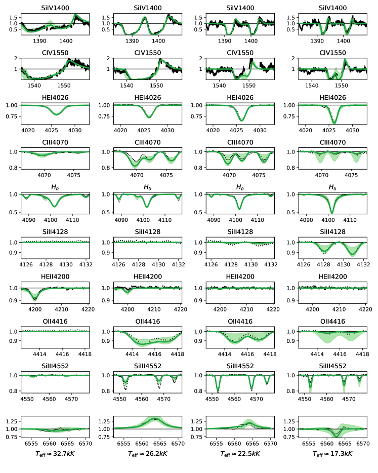
Figure 2: Comparison of diagnostic lines for 4 stars. The stars (Sk$-67^{\circ}107$, Sk$-68^{\circ}41$,Sk$-69^{\circ}52$,RMC-109) are organised from high (left) to low (right) effective temperature (in spectral type: O8.5 II, B0.7 Ia, B2 Ia, B5 Ia ). The lines are selected due to their roles as good diagnostics for stellar or wind parameters. From top to bottom the lines are sorted by wavelength. Note that the line names here correspond to the names in table LABEL:tab:linelist. The green line shows the best fit and the green shaded region shows the 1-$\sigma$ uncertainty interval.

2.7 Stellar parameter determinations

Not all parameters we are interested in are direct fit-parameters. There are a couple of extra parameters we can derive which are of particular interest, including: the mass, the radius, and $\Gamma_{\rm e}$. The mass can be obtained using

$$M_{\star}=\frac{g_{\star}R_{\star}^{2}}{G},$$ (7)

where $G$ is Newton’s gravitational constant and $g_{\star}$ is the surface gravity corrected for centrifugal effects ($g_{\star}=g_{\rm eff}+(\varv_{\rm rot}\sin i)^{2}/R_{\star}$). The stellar radius $R_{\star}$ is derived by using the fitted temperature and photometrically obtained stellar luminosity in the K-band (Vink et al. 2023), which we de-reddened. Shifting this apparent magnitude to absolute magnitude is then readily done using the distance modulus to the LMC set to 18.48 (Pietrzyński et al. 2019). The de-reddening will influence this luminosity anchor very little as the K-band extinction is low and thermal emission by dust only becomes relevant at longer wavelengths. When investigating how the K-band reddening influences the mass-loss rate we have computed that a change of 0.1 magnitude in the K-band luminosity results in only an 8% change in the mass-loss rate. This is thus lower than the expected error due to the depth of the LMC, which is on the order of 16% (Subramanian & Subramaniam 2009), and the typical errors of our fits are on the order of a factor 2. With these values we only need to find the radius for which the luminosity in the chosen band matches the observations.

Obtaining good estimates of stellar masses is also important for the wind analysis, since wind strength scales strongly with the classical Eddington parameter:

$$\Gamma_{\rm e}=\frac{\kappa_{e}L_{\star}}{4\pi cGM_{\star}},$$ (8)

with $\kappa_{\rm e}$ the electron scattering opacity and c the speed of light; $\Gamma_{\rm e}$ gives the ratio of radiative to gravitational acceleration in the case that the only opacity source is $\kappa_{e}$. When including these parameters on the various plots illustrating our results, we adopt

$$\kappa_{e}=\frac{\sigma_{T}}{m_{\rm H}}\left(\frac{1+I_{\rm He}\cdot Y_{\rm He}}{1+4\cdot{Y_{\rm He}}}\right).$$ (9)

Here $\sigma_{T}$ is the Thomson cross section, $m_{\rm H}$ is the mass of hydrogen, $I_{\rm He}$ is the ionisation of He giving either 1 or 2 free electrons for each He-atom (set to 1 for all B-stars in our sample and 2 for the O-stars); hydrogen is assumed to be fully ionised, and $Y_{He}$ is the helium to hydrogen number abundance ratio. Note that $\Gamma_{\rm e}$ does not take into account the line-driving effect of the radiation acceleration, but instead gives a generic radius independent value as a measure of the closeness of the star to the classical Eddington limit.

3 Results

In this section we present the stellar and wind parameters determined by the fitting method described above, applied to the sample of LMC stars. All the derived parameters and corresponding error estimates are given in tables 2, 3, and 4.

Figure 2 illustrates fits for a selection of important lines for four typical stars in our sample. The stars are organised from hot to cold, as clearly visible in the He ii lines which are present for the hottest star, but disappear when moving to the cooler objects. For the cooler stars the Si ii lines instead become stronger, while the Si iv line which is present in the red wing of the $H{\delta}$ line vanishes. The H ${\alpha}$ line for all stars shows clear signatures of wind emission filling in the photospheric absorption component, indicating this line is a good mass-loss indicator throughout our sample (though see discussion below on some complicating factors). All four stars show P-Cygni like features in the UV Si iv and C iv lines, again indicating the presence of significant wind outflows. In this respect, we note that C iv is clearly present in the wind of objects at around 17kK (although the doublet line there is narrower and weaker than in the other two stars); we discuss this further in Sect. 3.3, as it has consequences for our modelling of the wind ionisation balance and derivation of terminal wind speeds in this regime.

3.1 Stellar parameters

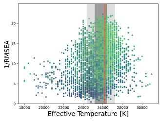
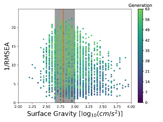
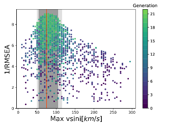
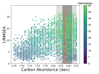
Figure 3: Distribution of the quality of the fits for stellar parameters of star Sk$-68^{\circ}41$. In dark grey the 1-$\sigma$ interval is shown while the light grey shows the 2-$\sigma$ interval. The red line shows the best fit value. We only display the C-abundance as the other elements have similar fitting curves. As mentioned in section 2.3 and the following sections we derive the maximum projected rotational velocity from the optical-only fit which is why there are only 21 generations.

Although our analysis and discussion will be focused mostly on wind parameters, we start by presenting the stellar parameters in table 1. We fit seven stellar parameters in our models, namely the effective temperature ($T_{\rm eff}$), the effective gravity at the stellar surface ($\log g$), a maximum (see further below) projected equatorial rotational velocity ($\varv_{\rm rot}\sin i$), the surface helium abundance ($Y_{\rm He}$) and the surface carbon, oxygen, and nitrogen (CNO) abundances. Figure 3 shows stellar parameter distributions of the inverse of RMSEA for models of a characteristic star in our sample. The best fit values are marked with a red line and the 1- and 2-$\sigma$ confidence intervals are the dark and light grey shaded regions. The colour scheme marks which generation in the GA the model stems from. We see that the distributions for effective temperature, surface gravity, and maximum $\varv_{\rm rot}\sin i$ all have well-defined and fairly sharp peaks in their distributions, suggesting good statistical constraints on the parameters. The abundances are generally more difficult to constrain, but also these sometimes display relatively peaked distributions, as exemplified for carbon in the figure.

The sensitivity to effective temperature of the GA is best constrained from the silicon lines, as well as helium lines for stars on the hotter end of our sample. We note that other lines are sensitive to $T_{\rm eff}$ and that due to the nature of a GA all of these are taken into account when deriving the best fit and the uncertainty margins. For all stars in the sample we see a strongly peaked distribution for the effective temperature meaning that the combination of stellar lines is adequate for determining $T_{\rm eff}$. The derived effective temperatures for the sample range from about 15 kK to 30 kK with luminosities ranging from $4.7-5.8\log_{10}(L/L_{\odot})$. Figure 4 shows the stars in the Hertzsprung-Russell Diagram (HRD) with their spectroscopic mass indicated by their colour. We have plotted the evolutionary tracks from the MIST data base (Dotter 2016; Choi et al. 2016; Paxton et al. 2010, 2013, 2015) for a 15, 26, and 40 $M_{\odot}$ star in the same window. Comparing these models to our spectroscopic results, the majority of our sample appears to be in the post-main sequence phase of evolution. We note, however, that the evolutionary tracks shown in the figure assume a convective core overshoot parameter $f_{\rm ov,core}=0.2$ for a step overshoot model (Choi et al. 2016); if stronger overshooting would be assumed this might extend the main sequence so that some of the stars in the sample could still be on it (Castro et al. 2014).

The derived surface gravities are presented in table 2. For which, in particular $H{\gamma},H{\delta}$ are sensitive. The fit values for $\log_{10}$ (g   $\text{cm}/\text{s}^{2})$ range from 2.2 to 3.6. Only four stars in our sample have a surface gravity $3.0<\log_{10}(g\,\text{cm}/\text{s}^{2})$.

Surface gravity is an important stellar parameter because of its direct influence on the derived spectroscopic mass of the star as described in section 2.7. The resulting derived spectral masses from these surface gravities lie between between 15 and 75 $M_{\odot}$, with corresponding stellar radii between 19 and 70 $R_{\odot}$. The latter are shown by the colour scheme in the HR-diagram of figure 4. $\Gamma_{\rm e}$ in this sample ranges from 0.10 to 0.46. This parameter is important for the analysis below as it represents another key axis over which wind behaviour changes, in addition to the temperature axis.

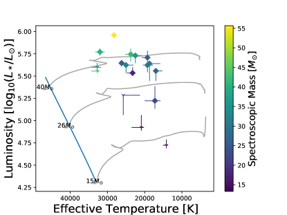
Figure 4: HR-diagram showing all stars in the sample with the colour showing the derived spectral masses. The diamonds mark all the stars with spectral types Ia while the ’v’ mark the lower luminosity classes. The stellar evolution tracks are from the MIST data base without any rotation (Dotter 2016; Choi et al. 2016; Paxton et al. 2010, 2013, 2015)

The maximum projected stellar rotation (max $\varv_{\rm rot}\sin{i}$) is the only macroscopic broadening mechanism included in our line fits, meaning we do not attempt here to differentiate between different macroscopic broadening mechanisms (e.g. rotation and ’macro-turbulence’). As such, the quoted $\varv_{\rm rot}\sin{i}$ values are upper limits, and not the actual projected equatorial rotation velocity (as its measurement is influenced by the broadening mechanisms we do not handle explicitly). Figure 5 shows the derived upper limits of $\varv_{\rm rot}\sin i$ as function of the effective temperature. We note that, with the exception of three of the hottest objects, our sample has max $(\varv_{\rm rot}\sin i)<100\,\rm km/s$. Indeed, it is for these relatively low values that we expect it to be difficult to disentangle rotation broadening from other macroscopic broadening mechanisms. Specifically, Sundqvist et al. (2013) showed that when applying standard techniques to disentangle effects from macro-turbulence $\varv_{\rm mac}$ and $\varv_{\rm rot}\sin{i}$ for massive stars with known very long rotation periods, corresponding to $\varv_{\rm rot}\sin{i}\la 1$ km/s, one still ends up deriving $\varv_{\rm rot}\sin{i}\sim\varv_{\rm mac}$ whenever significant macro-turbulence is present in the observational data. This demonstrates the difficulty of present methods to disentangle these two effects, motivating our methodological choice here (indeed, visual inspection of our observed strategic line-profiles often show more Gaussian-like shapes than the rounded shape predicted by broadening due to rotation). That is, our quoted values for max $\varv_{\rm rot}\sin{i}$ may as well reflect the presence of large Gaussian-like turbulent motions and not stellar rotation.

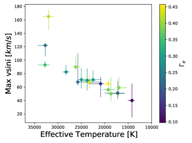
Figure 5: Derived maximum projected rotational velocity in function of effective temperature. Note that this maximum value in practice reflects the combined effect of all sources of macroscopic line broadening (see text).

The average helium abundance is $Y_{\rm He}=0.1$ (or alternatively $\epsilon_{\rm He}=11.0$, see below) with the highest and lowest values of the helium abundance 1 dex apart ($\epsilon_{\rm He}\approx 11.4-10.4$) with relative small error margins on the order of 0.2 dex. As one may have noted table 2 shows values which reach helium abundances below $Y_{\rm He}=0.08$. This might seem problematic as this is below the expected baseline for the LMC at $y=0.091_{-0.012}^{+0.014}$ (Russell & Dopita 1990). However, the fitting range in all cases reaches values above this 0.08 baseline and as mentioned above, this range is the important property to assess. We have refitted all problematic stars, as a test, while not allowing the helium abundance to be lower than $Y_{\rm He}=0.08$ and no values change appreciatively from table 2.

Finally, to make the GA sensitive to CNO-abundances, we added atmospheric CNO lines of various ionisation stages. However, because this paper makes an effort to focus on mass-loss rates and not on abundances there are comparatively few data points which are sensitive to the abundance. As such, small changes to a specific abundance only modify the quality of the fit of these specific lines slightly (for instance we include only one NII quintuplet) and typically do not affect significantly the overall fit quality used to define our ’best-fit’ model. Consequently, we see high uncertainty regions in CNO abundance as compared to the other stellar parameters. The abundances of CNO in this paper are given on the standard scale $\epsilon_{\rm x}=12+\log_{10}(n_{\rm x}/n_{\rm H})$ where $n_{\rm H}$ is the number abundance of hydrogen abundance and $n_{x}$ is the number abundance of the element. The average CNO abundances we find for our sample are $\epsilon_{\rm C}=8.0,\epsilon_{\rm N}=7.2,\epsilon_{\rm O}=8.3$. Although these are fitted using different lines they do display similar behaviour for their error margins, which are typically on the order of 0.5-1 dex for all elements. Abundances and 1-$\sigma$ error margins for each star in our sample are given in table 2. Vink et al. (2023) gathered abundances of common elements in the LMC and averaged the abundances found in different stellar populations to find $\epsilon_{\rm C}=8.01,\epsilon_{\rm N}=7.03,\epsilon_{\rm O}=8.4$; in comparison to these results, we appear to have relative agreement. However, the uncertainty of our derived abundances is usually on the order of 0.5-1 dex. 5 of the stars in our sample have been studied in the optical regime by Menon et al. (2024) focusing on the CNO abundances to determine if they are possible binary merger products. All of the stellar parameters (e.g., $T_{\rm eff}$ and $\log{g}$) have overlap in the error-margins, however for some of the CNO abundances we find drastically different best-fit solutions. Due to the very big uncertainty intervals on our CNO-abundances we do still overlap in most cases, but as mentioned above getting close constraints on CNO-abundances has not been our focus. For a small expansion on our derived CNO abundance see figure 18.

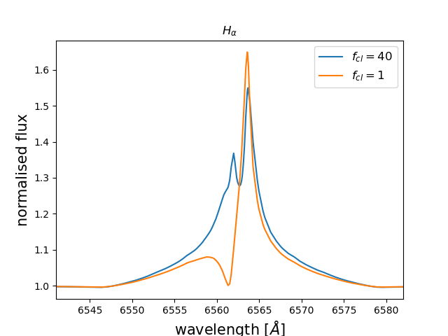
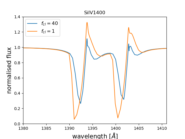
Figure 6: Clumping influence on the spectral lines. The figures show the influence a change in $f_{\rm cl}$ has on the line profile of on one hand the H ${\alpha}$ recombination line and on the other hand the Si iv 1400 resonance doublet. Both model spectra are using almost the same input, they only differ in mass-loss rate and clumping. The blue line both has $\dot{M}=8\cdot 10^{-8}M_{\odot}$/yr, and is highly clumped ($f_{\rm cl}=40$). The orange line is a smooth outflow but has a significantly higher mass-loss rate ($\dot{M}=5\cdot 10^{-7}M_{\odot}$/yr); the product $\sqrt{f_{\rm cl}}\dot{M}$ is thus the same for both lines. If we assume an optically thin clumping over the complete line forming region, the 2 H ${\alpha}$ lines would show perfect agreement. However, this is not the case as we use models that relax the optically thin assumption and are only clumped above a fitted onset-velocity.

3.2 Mass-loss rates

H ${\alpha}$ is the a sensitive mass-loss diagnostic. However, it is important to realise here that since H ${\alpha}$ is a recombination line in this regime, the line is also sensitive to the wind-clumping factor $f_{\rm cl}$. Additionally, it has been suggested by Petrov et al. (2014) that the H ${\alpha}$ line behaviour and morphology may change with temperature around the supposed bistability jump. If $f_{\rm cl}$ would be kept constant throughout the complete line-forming region, and clumps would be optically thin, the scaling invariant would simply be $\sqrt{f_{\rm cl}}\dot{M}$. However, since H ${\alpha}$ often is formed in the region where wind clumping starts to become effective in our models (i.e. in regions around $\varv_{\rm cl,start}$ and between $\varv_{\rm cl,start}$ and $\varv_{\rm cl,max}$), deviations from this basic scaling may occur. Even so, the degeneracy between $f_{\rm cl}$ and $\dot{M}$ causes problems when trying to determine absolute mass-loss rates using only the strength of H ${\alpha}$. Figure 6 illustrates H ${\alpha}$’s strong dependency on mass loss and the corresponding degeneracy with $f_{\rm cl}$. Both stars in figure 6 have the same input parameters (specifically $T_{\rm eff}=20$kK, $\log_{10}g=2.7$, $\varv_{\infty}=750$ km/s, $f_{\rm ic}=0.1$, $f_{\rm vel}=0.5$), except for the mass-loss rate and clumping factor. The orange line is for a smooth outflow and $\dot{M}=5\cdot 10^{-7}M_{\odot}$/yr, and the blue line has $f_{\rm cl}=40$ and $\dot{M}=8\cdot 10^{-8}M_{\odot}/$yr. The mass-loss rate is thus different for both stars, but the product $\sqrt{f_{\rm cl}}\dot{M}$ is the same. One can see that the height of the peak of the $H{\alpha}$ line is similar in the two models. The match is not perfect, however, and the overall shape is different, because the H ${\alpha}$ line is partly formed in regions where $f_{\rm cl}$ has not reached its maximum value (here we have assumed $\varv_{\rm cl,start}=0.05$ and $\varv_{\rm cl,max}=0.1$ for both model stars). In the optically thin limit and assuming the clumping is constant over the entire velocity range the 2 H ${\alpha}$ profiles would match perfectly, but the models we use here relax these assumptions. In an attempt to break this mass loss-clumping degeneracy, we fit not only the sensitive H ${\alpha}$ line but also wind resonance lines in the UV. These often depend differently on wind clumping as their extinction coefficients typically scale as $\sim\langle\rho\rangle$, rather than $\sim\langle\rho^{2}\rangle$ as in the case of recombination lines. We note that additional dependencies from the ionisation balance and velocity-porosity effects (as well as saturation and interclump density effects) can modify these natural scalings of recombination and resonance lines, making it complicated to sort out all inter-dependencies. We show this in the lower panel of figure 6, displaying the Si IV resonance doublet for the same stars and parameter combinations as the H ${\alpha}$ line discussed above; it is clear that the dependence on $f_{\rm cl}$ is very different for these lines than for H ${\alpha}$. Specifically for this case, we now observe how the absorption troughs in the doublet lines become weaker for an increasing $f_{\rm cl}$, which here is because the ionisation balance of silicon shifts when strong clumping is introduced. In our multi-diagnostic automated fits we utilise these kind of differences in how lines react to derive simultaneous constraints on $f_{\rm cl}$ and $\dot{M}$ (and the other stellar and wind parameters).

Overall, our multi-diagnostic GA approach is able to isolate the mass-loss dependence rather well and so derive absolute values of $\dot{M}$. This is demonstrated in Figure 7, showing the distribution of the inverse of RMSEA for models of the same star but with different mass-loss rates. The more peaked this distribution is, the better the GA can distinguish the different parameter values from each other.The GA method takes into account the interactions of all degeneracies automatically when deriving uncertainty intervals. In the cases where the clumping factor stays somewhat degenerate with the mass-loss rate we see a broadness in both the mass loss and derived clumping factor. This is more common in the low temperature stars. Best-fitting mass-loss rates for all stars in our sample are shown in figure 12 and vary from $\sim 10^{-6}M_{\odot}/\text{yr}$ for the hotter stars to $\sim 10^{-8}M_{\odot}/\text{yr}$ for the cooler stars. Figure 8 further displays the correlation between $\dot{M}$ and $f_{\rm cl}$ for the fit of star Sk$-68^{\circ}41$, showing 1/RMSEA for each combination of clumping factor and mass-loss rate (note that one such combination may have several models due to variation in other parameters). Due to the sparse sampling there is some stochasticity in the RMSEA values. The figure illustrates that although the uncertainty in $f_{\rm cl}$ is rather high, no severe degeneracy issues between $f_{\rm cl}$ and $\dot{M}$ seem to be present in our fits as there is a clear optimal region.

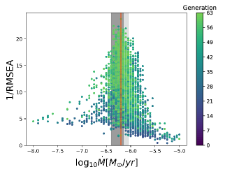
Figure 7: Quality of all models in a GA run ranked based on the inverse of the RMSEA value as a function of the mass-loss rate. The models for these plot are based on a run trying to fit the star Sk$-68^{\circ}41$ (SpT B0.7 Ia). Each point here is a separate model where the colour defines the generation in which this model was run. The dark grey region highlights the 1-$\sigma$ uncertainty interval and the light grey region is the 2-$\sigma$ uncertainty.

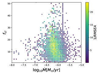
Figure 8: Correlation between the clumping factor and the mass-loss rate for star sk$-68^{\circ}41$. The colour shows the 1/RMSEA value.

3.3 Wind speeds, accelerations, and turbulence

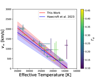
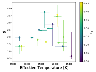
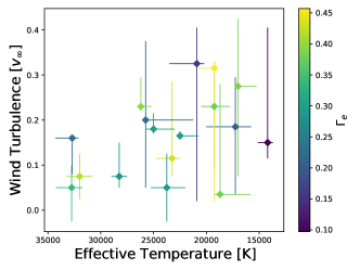
Figure 9: Derived terminal velocities, wind acceleration parameter $\beta$, and maximum wind micro-turbulence, as function of effective temperature. colour for all panels shows the $\Gamma_{\rm e}$ value. The first panel also shows a linear fit to the terminal velocities found in this work in red compared to the fit in blue from Hawcroft et al. (2024b).

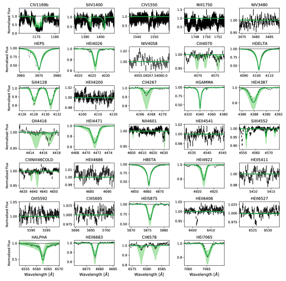
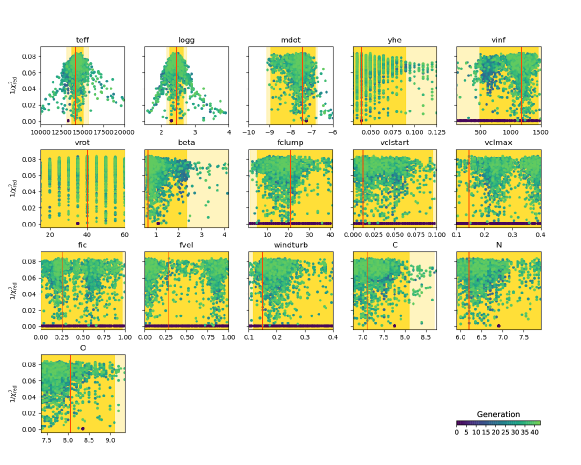
Figure 37: Same as figure 21 but for object Sk$-67^{\circ}195$.

The lines that provide a good diagnostic of terminal wind speed to the GA fits are Si iv 1400 and C iv1550. These lines often appear as distinct ’P-Cygni’ profiles, allowing for fairly straightforward visual verification of the fitted $\varv_{\infty}$ from the broadness of their blue-shifted absorption. The dependence of the strength of these lines on temperature can be seen in figure 2, where a few characteristic lines are shown for four stars ranging from high (left) to low (right) effective temperature. The observed C iv and Si iv lines for higher $T_{\rm eff}$ are well-developed, strong or even saturated towards the blue absorption edge. The features become less broad when reducing the temperature, which generally points to lower terminal velocity. In the standard modelling of the cooler stars in our sample, C iv is actually no longer present in the wind. Nonetheless, as seen in figure 2, some of these cool stars still display significant observed P-Cygni profiles for C iv1550 (albeit weaker than for the hotter objects). To reproduce this behaviour in the modelling, we have included X-rays in the fastwind simulations also in this temperature region (previous versions did not consider X-ray ionisation below $T_{\rm eff}\sim 25$ kK), which then can raise the wind ionisation balance and produce enough C iv to explain the observed lines. The influence of these X-rays upon the determination of $\varv_{\infty}$ in this parameter range is further discussed below. The terminal wind speeds resulting from our fits of the full sample are displayed in panel 1 of figure 9 as a function of effective temperature. For the coolest star in our sample (Sk$-67^{\circ}195$) all UV-lines which are sensitive to the terminal wind speed are no longer present. As a result, we do not get good constraints on the terminal wind speed this is also shown in the fit-distribution in figure 37, which is flat.

The wind acceleration is parametrised by the $\beta$ value in the analytic velocity law (see previous section). As can be seen in panel 2 of figure 9, we find relatively high values $\ga 1.5$, with a sample average $\langle\beta\rangle=2.1$. This is significantly higher than values derived for hotter O-stars by B22, who found an average $\beta\la 1.0$ in that regime, but comparable to the optical only BSG study in the Galaxy by Haucke et al. (2018) and the UV+optical SMC BSG study by Bernini-Peron et al. (2024). Overall, the slower wind acceleration we find for BSGs compared to the faster wind acceleration found for early O-stars agree well with a range of previous studies (overview in Puls et al. 2008). The error margins on these values are appreciable but still keep the 1-$\sigma$ error interval clear above 1. A larger scatter is seen for the cooler stars in the sample.

The inferred values of maximum wind micro-turbulence range from 0.05 to 0.4 in units of $\varv_{\infty}$, with a sample average 0.2. The uncertainty interval of this fit parameter is generally high with typical errors around 0.1, but with outliers reaching error margins as high as 0.4 on this scale. We note that this value then also has a significant effect of the derived terminal wind speed, as turbulence adds to the blueward extension of the modelled line-profile.

3.4 Clumping

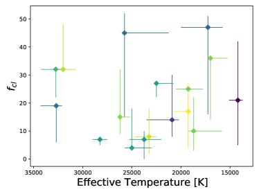
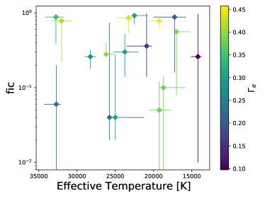
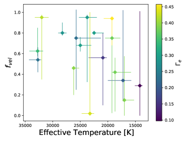
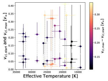
Figure 10: Clumping parameters with respect to the effective temperature. The panels from top left to bottom right show the clumping factor, interclump density (in units of mean density), velocity filling factor and the onset clumping velocity ($\varv_{\rm cl,start}$) and the velocity of maximum clumping ($\varv_{\rm cl,max}$). The 3 first panels colour according to $\Gamma_{\rm e}$ for the stars, while in the last plot the colour indicates the difference between $\varv_{\rm cl,start}$ and $\varv_{\rm cl,max}$. For each star in this plot the 2 points are connected by a dashed line (not visible in some objects as the error margins are covering the dashed line).

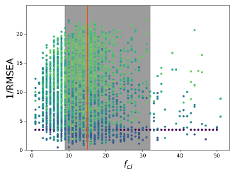
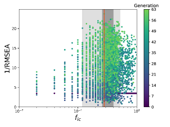
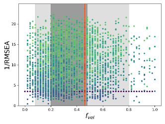
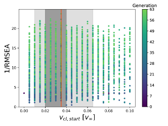
Figure 11: Distribution of the quality of the fits for clumping parameters. We show a typical distribution of the models at end of a GA fitting run. Here the colour indicates the generation of the model and the grey areas indicate the 1- and 2-$\sigma$ uncertainty intervals.

To recapitulate, in addition to the clumping factor ($f_{\rm cl}$), we fit the interclump-density parameter $f_{\rm ic}$, the velocity filling factor $f_{\rm vel}$, the onset of clumping $\varv_{\rm cl,start}$, and the wind speed at which maximum values for the clumping parameters are reached $\varv_{\rm cl,max}$. All parameter-values displayed in figures and quoted in text are the maximum values, applied in our models from $\varv_{\rm cl,max}$ to the outer boundary. As also found in the previous studies by H21 and B22 it is generally challenging to obtain simultaneous constraints on these parameters.

Figure 10 shows the determined clumping parameters as function of effective temperature. The plots are generally characterised by significant scatter and large error-bars, illustrating the general challenge of obtaining these parameter values or finding a trend with temperature. Within 1-$\sigma$ errors, clumping factors range between the lower limit 1 up to $\sim$ 40 for our sample and velocity filling factors between very low values $\la 0.1$ all the way up to the upper limit unity. While the scatter in interclump density is high, this parameter does seem to show some preference for values $\ga 0.1$. $\varv_{\rm cl,start}$ is generally preferred to have wind clumping start rather close to our lower allowed bound at $\varv_{\rm cl,start}\approx a$, although the scatter in this parameter is high with typical values within 1-$\sigma$ ranging from $\varv_{\rm cl,start}/\varv_{\infty}\la 0.01$ up to $\sim 0.1$. $\varv_{\rm cl,max}$ typically is about $\sim 0.2\varv_{\infty}$, with similarly broad ranges including a few outliers at the high end reaching values of 0.35; the 1-$\sigma$ interval for this parameter ranges from 0.05 to 0.15 $\varv_{\infty}$. Additionally, panel four in figure 10 uses colour to show the difference between $\varv_{\rm cl,max}$ and $\varv_{\rm cl,start}$, where we find that most stars have values $\varv_{\rm cl,max}-\varv_{\rm cl,start}\approx 0.2$ in units of $\varv_{\infty}$.

Table 2: Best fit photospheric parameters of the sample stars.

object	SpT	$T_{\rm eff}$[K]	$g_{\rm eff}$ [$\log_{10}(cm/s^{2})$]	$y_{\rm He}[n_{He}/n_{H}]$	$\varv_{\text{max, vsini}}[km/s]$	C [dex]	N [dex]	O [dex]
Sk$-67^{\circ}195$	B6 I	$14200_{-500}^{+900}$	$2.45_{-0.2}^{+0.2}$	$0.04_{-0.02}^{+0.05}$	$40_{-25}^{+25}$	$7.1_{-0.4}^{+1.0}$	$6.2_{-0.35}^{+1.75}$	$8.05_{-0.75}^{+1.05}$
Sk$-68^{\circ}8$	B5 Ia+	$17000_{-1750}^{+250}$	$2.15_{-0.25}^{+0.05}$	$0.05_{-0.03}^{+0.08}$	$59_{-13}^{+16}$	$7.35_{-0.4}^{+1.1}$	$7.85_{-1.0}^{+0.1}$	$8.45_{-0.6}^{+0.95}$
RMC-109	B5 Ia	$17250_{-1500}^{+2750}$	$2.45_{-0.35}^{+0.4}$	$0.05_{-0.0}^{+0.08}$	$51_{-9}^{+18}$	$8.5_{-0.2}^{+0.25}$	$6.35_{-0.5}^{+0.6}$	$7.6_{-0.25}^{+0.4}$
Sk$-67^{\circ}78$	B3 Ia	$19250_{-1500}^{+1250}$	$2.35_{-0.1}^{+0.2}$	$0.08_{-0.02}^{+0.03}$	$56_{-2}^{+14}$	$7.2_{-0.5}^{+0.6}$	$7.85_{-1.05}^{+0.15}$	$8.9_{-1.4}^{+0.2}$
Sk$-70^{\circ}50$	B3 Ia	$18700_{-2900}^{+600}$	$2.3_{-0.35}^{+0.2}$	$0.08_{-0.02}^{+0.01}$	$50_{-10}^{+25}$	$7.85_{-0.05}^{+0.5}$	$7.3_{-1.1}^{+0.8}$	$7.9_{-0.2}^{+0.7}$
Sk$-68^{\circ}26$	B2 Ia	$19250_{-250}^{+1500}$	$2.2_{-0.05}^{+0.2}$	$0.16_{-0.05}^{+0.01}$	$65_{-11}^{+5}$	$8.45_{-0.55}^{+0.25}$	$7.4_{-0.35}^{+0.05}$	$8.3_{-0.05}^{+0.55}$
Sk$-70^{\circ}16$	B2 II	$20900_{-700}^{+2600}$	$2.85_{-0.2}^{+0.25}$	$0.1_{-0.05}^{+0.04}$	$65_{-20}^{+10}$	$8.2_{-0.25}^{+0.15}$	$8.35_{-0.55}^{+0.5}$	$8.82_{-1.02}^{+0.03}$
Sk$-69^{\circ}52$	B2 Ia	$22500_{-1750}^{+250}$	$2.6_{-0.1}^{+0.05}$	$0.26_{-0.09}^{+0.01}$	$71_{-1}^{+14}$	$8.35_{-0.1}^{+0.05}$	$7.55_{-0.05}^{+0.35}$	$8.45_{-0.2}^{+0.05}$
Sk$-67^{\circ}14$	B1 Ia	$23250_{-750}^{+1500}$	$2.55_{-0.05}^{+0.35}$	$0.16_{-0.12}^{+0.04}$	$67_{-10}^{+11}$	$8.4_{-0.8}^{+0.05}$	$7.15_{-0.05}^{+1.5}$	$8.7_{-0.45}^{+0.05}$
Sk$-69^{\circ}140$	B1 Ib	$25750_{-4500}^{+250}$	$3.05_{-0.4}^{+0.15}$	$0.11_{-0.02}^{+0.06}$	$68_{-5}^{+42}$	$8.45_{-0.3}^{+0.35}$	$6.1_{-0.2}^{+1.45}$	$7.8_{-0.25}^{+1.3}$
Sk$-66^{\circ}35$	BC1 Iab	$23750_{-1750}^{+1500}$	$2.75_{-0.1}^{+0.55}$	$0.18_{-0.08}^{+0.01}$	$70_{-15}^{+18}$	$8.4_{-0.4}^{+0.35}$	$7.45_{-1.15}^{+0.4}$	$8.5_{-0.4}^{+0.5}$
Sk$-69^{\circ}43$	B0.7 Ia	$25000_{-2000}^{+750}$	$2.85_{-0.25}^{+0.05}$	$0.14_{-0.02}^{+0.09}$	$71_{-13}^{+17}$	$7.95_{-0.25}^{+0.15}$	$7.35_{-0.2}^{+0.6}$	$9.25_{-0.9}^{+0.15}$
Sk$-68^{\circ}41$	B0.7 Ia	$26200_{-1000}^{+200}$	$2.8_{-0.15}^{+0.2}$	$0.16_{-0.04}^{+0.01}$	$90_{-5}^{+15}$	$8.35_{-0.05}^{+0.25}$	$7.6_{-0.05}^{+0.65}$	$9.25_{-0.5}^{+0.05}$
Sk$-68^{\circ}52$	B0 Ia	$28250_{-750}^{+750}$	$3.1_{-0.1}^{+0.25}$	$0.13_{-0.03}^{+0.02}$	$82_{-5}^{+10}$	$8.55_{-0.1}^{+0.15}$	$7.5_{-1.05}^{+0.2}$	$7.75_{-0.4}^{+0.05}$
Sk$-68^{\circ}155$	O9 Ia	$32000_{-1250}^{+1250}$	$3.2_{-0.25}^{+0.2}$	$0.12_{-0.02}^{+0.03}$	$165_{-20}^{+10}$	$7.1_{-0.05}^{+1.05}$	$7.15_{-0.05}^{+0.7}$	$8.25_{-0.05}^{+0.65}$
Sk$-67^{\circ}107$	O8.5 II	$32750_{-1000}^{+1500}$	$3.35_{-0.25}^{+0.15}$	$0.08_{-0.01}^{+0.06}$	$93_{-4}^{+6}$	$8.05_{-0.1}^{+0.25}$	$6.55_{-0.4}^{+0.1}$	$7.6_{-0.25}^{+1.05}$
Sk$-67^{\circ}106$	O8 II	$32700_{-600}^{+1600}$	$3.5_{-0.15}^{+0.5}$	$0.11_{-0.03}^{+0.01}$	$122_{-16}^{+1}$	$7.7_{-0.45}^{+0.2}$	$6.25_{-0.1}^{+0.7}$	$7.75_{-0.05}^{+0.45}$

• Notes: For $y_{\rm He}$ and $\varv_{\text{max, vsini}}$ we show the errors of the optical only fits, as their fit range has been constrained for the full UV and optical fit.

Table 3: Derived and X-ray parameters of all objects in our sample.

object	$M_{\text{spec}}[M_{\odot}]$	$M_{\text{evo}}[M_{\odot}]$	$\log_{10}(L/L_{\odot})$	Radius$[R_{\odot}]$	$\Gamma_{\rm e}$	$u_{\infty}[km/s]$	$\log_{10}$($f_{x}$)	$\log_{10}(L_{x}/L_{\text{bol}})$
Sk$-67^{\circ}195$	$15.43_{-4.49}^{+5.4}$	N/A	$4.72_{-0.03}^{+0.06}$	$38.33_{-1.32}^{+0.71}$	$0.1_{-0.02}^{+0.05}$	N/A	N/A	N/A
Sk$-68^{\circ}8$	$26.45_{-6.89}^{+1.93}$	$32.0^{+2.15}_{-3.28}$	$5.56_{-0.11}^{+0.0}$	$69.89_{-0.0}^{+4.13}$	$0.39_{-0.09}^{+0.03}$	$175.0_{-175.0}^{+325.0}$	$-1.95_{-0.1}^{+0.95}$	$-10.34_{-23.41}^{+3.31}$
RMC-109	$22.56_{-9.48}^{+21.33}$	$22.0^{+4.01}_{-2.34}$	$5.22_{-0.09}^{+0.16}$	$46.18_{-3.64}^{+2.21}$	$0.21_{-0.08}^{+0.07}$	$505.0_{-375.0}^{+87.5}$	$0.4_{-0.65}^{+0.65}$	$-6.1_{-3.03}^{+0.0}$
Sk$-67^{\circ}78$	$29.22_{-2.1}^{+9.28}$	$30.0^{+2.49}_{-1.17}$	$5.62_{-0.08}^{+0.06}$	$58.82_{-1.76}^{+2.44}$	$0.38_{-0.1}^{+0.0}$	$625.0_{-125.0}^{+325.0}$	$0.25_{-0.95}^{+0.05}$	$-5.69_{-1.38}^{+0.02}$
Sk$-70^{\circ}50$	$30.23_{-10.44}^{+11.38}$	$31.2^{+2.74}_{-2.77}$	$5.64_{-0.2}^{+0.03}$	$63.55_{-1.0}^{+6.67}$	$0.38_{-0.09}^{+0.02}$	$175.0_{-25.0}^{+775.0}$	$-0.2_{-1.3}^{+0.05}$	$-8.35_{-0.41}^{+1.39}$
Sk$-68^{\circ}26$	$25.71_{-2.2}^{+10.19}$	$38.4^{+3.3}_{-2.31}$	$5.71_{-0.0}^{+0.08}$	$64.79_{-2.39}^{+0.0}$	$0.46_{-0.12}^{+0.17}$	$600.0_{-25.0}^{+275.0}$	$-1.4_{-0.65}^{+0.55}$	$-7.53_{-0.21}^{+0.66}$
Sk$-70^{\circ}16$	$13.33_{-3.61}^{+5.16}$	$17.0^{+1.71}_{-1.03}$	$4.92_{-0.04}^{+0.14}$	$22.29_{-1.43}^{+0.39}$	$0.16_{-0.03}^{+0.05}$	$517.5_{-125.0}^{+50.0}$	$0.88_{-0.03}^{+0.35}$	$-5.72_{-2.44}^{+0.32}$
Sk$-69^{\circ}52$	$35.69_{-0.55}^{+0.0}$	$36.0^{+2.18}_{-3.24}$	$5.73_{-0.08}^{+0.0}$	$48.67_{-0.0}^{+2.02}$	$0.3_{-0.01}^{+0.0}$	$675.0_{-425.0}^{+25.0}$	$-1.9_{-0.05}^{+0.1}$	$-7.92_{-0.98}^{+0.0}$
Sk$-67^{\circ}14$	$18.0_{-0.0}^{+18.22}$	$31.4^{+2.01}_{-1.95}$	$5.53_{-0.03}^{+0.06}$	$36.39_{-1.1}^{+0.46}$	$0.43_{-0.19}^{+0.0}$	$425.0_{-350.0}^{+25.0}$	$-1.0_{-0.45}^{+1.7}$	$-6.82_{-2.68}^{+0.0}$
Sk$-69^{\circ}140$	$20.80_{-10.08}^{+7.72}$	$37.8^{+2.76}_{-2.94}$	$5.28_{-0.22}^{+0.0}$	$22.25_{-0.0}^{+2.46}$	$0.23_{-0.1}^{+0.11}$	$350.0_{-150.0}^{+550.0}$	$-0.1_{-0.45}^{+0.35}$	$-7.51_{-1.18}^{+0.88}$
Sk$-66^{\circ}35$	$41.62_{-3.96}^{+85.6}$	$38.80^{+3.25}_{-2.86}$	$5.74_{-0.08}^{+0.06}$	$44.42_{-1.3}^{+1.72}$	$0.29_{-0.19}^{+0.05}$	$150.0_{-75.0}^{+50.0}$	$0.05_{-0.25}^{+0.35}$	$-8.42_{-1.73}^{+0.28}$
Sk$-69^{\circ}43$	$32.34_{-10.1}^{+0.0}$	$32.8^{+2.27}_{-3.07}$	$5.62_{-0.09}^{+0.02}$	$34.88_{-0.39}^{+1.51}$	$0.3_{-0.03}^{+0.08}$	$650.0_{-200.0}^{+25.0}$	$-1.7_{-0.25}^{+0.5}$	$-7.07_{-0.78}^{+0.0}$
Sk$-68^{\circ}41$	$25.82_{-3.97}^{+10.38}$	$35.0^{+1.69}_{-1.89}$	$5.65_{-0.04}^{+0.0}$	$32.58_{-0.0}^{+0.58}$	$0.39_{-0.11}^{+0.05}$	$950.0_{-725.0}^{+25.0}$	$-1.3_{-0.05}^{+0.35}$	$-6.42_{-1.55}^{+0.0}$
Sk$-68^{\circ}52$	$75.65_{-6.61}^{+41.34}$	$56.00^{+2.38}_{-3.85}$	$5.96_{-0.02}^{+0.02}$	$40.2_{-0.4}^{+0.41}$	$0.28_{-0.09}^{+0.02}$	$225.0_{-175.0}^{+25.0}$	$-0.7_{-0.2}^{+1.05}$	$-7.83_{-3.99}^{+0.0}$
Sk$-68^{\circ}155$	$40.37_{-13.31}^{+13.57}$	$44.20^{+2.71}_{-3.74}$	$5.77_{-0.04}^{+0.04}$	$25.22_{-0.43}^{+0.45}$	$0.42_{-0.09}^{+0.18}$	$375.0_{-350.0}^{+325.0}$	$-0.55_{-0.05}^{+0.45}$	$-7.15_{-13.26}^{+0.98}$
Sk$-67^{\circ}107$	$32.82_{-11.14}^{+6.54}$	$37.4^{+0.0}_{-0.0}$	$5.6_{-0.03}^{+0.05}$	$19.77_{-0.41}^{+0.26}$	$0.34_{-0.06}^{+0.13}$	$475.0_{-375.0}^{+25.0}$	$0.35_{-0.25}^{+0.45}$	$-5.86_{-2.62}^{+0.0}$
Sk$-67^{\circ}106$	$42.46_{-9.15}^{+67.04}$	$36.0^{+1.96}_{-1.54}$	$5.56_{-0.01}^{+0.05}$	$18.85_{-0.59}^{+0.18}$	$0.23_{-0.13}^{+0.07}$	$375.0_{-25.0}^{+625.0}$	$-1.4_{-0.4}^{+0.2}$	$-8.11_{-0.01}^{+1.03}$

• Note: $\Gamma_{\rm e}$ is the classical Eddington parameter, $u_{\infty}$ is the maximum jump speed used to determine the X-ray characteristics, $\log_{10}(f_{x})$ is defined as $16e_{s}^{2}$ with $e_{s}$ the X-ray volume filling factor. $L_{x}/L_{\rm bol}$ is the X-ray luminosity scaled to the bolometric luminosity.

Table 4: Best fit wind parameters including optically thick clumping.

object	$\log_{10}\dot{M}[M_{\odot}/yr]$	$\varv_{\infty}[km/s]$	$\beta$	$f_{\rm cl}$	$f_{\rm ic}$	$f_{\rm vel}$	$\varv_{\text{cl, start}}[\varv_{\infty}]$	$\varv_{\text{cl, max}}[\varv_{\infty}]$	$\varv_{\text{turb}}$ [$\varv_{\infty}$]
Sk$-67^{\circ}195$	$-7.45_{-1.5}^{+0.6}$	$1180_{-700}^{+280}$	$0.65_{-0.2}^{+1.7}$	$21.0_{-16.0}^{+21.0}$	$0.26_{-0.25}^{+0.71}$	$0.29_{-0.29}^{+0.72}$	$0.01_{-0.01}^{+0.08}$	$0.14_{-0.04}^{+0.26}$	$0.15_{-0.04}^{+0.26}$
Sk$-68^{\circ}8$	$-7.1_{-0.35}^{+0.3}$	$400_{-350}^{+150}$	$2.0_{-1.0}^{+1.2}$	$36.0_{-22.0}^{+1.0}$	$0.56_{-0.48}^{+0.04}$	$0.15_{-0.15}^{+0.43}$	$0.06_{-0.06}^{+0.04}$	$0.18_{-0.04}^{+0.23}$	$0.28_{-0.2}^{+0.15}$
RMC-109	$-7.75_{-0.55}^{+0.5}$	$425_{-50}^{+100}$	$1.35_{-0.1}^{+0.8}$	$47.0_{-31.0}^{+4.0}$	$0.88_{-0.72}^{+0.04}$	$0.34_{-0.2}^{+0.68}$	$0.04_{-0.04}^{+0.06}$	$0.15_{-0.05}^{+0.13}$	$0.18_{-0.15}^{+0.11}$
Sk$-67^{\circ}78$	$-6.82_{-0.12}^{+0.28}$	$950_{-400}^{+350}$	$3.45_{-0.55}^{+0.8}$	$25.0_{-21.0}^{+1.0}$	$0.05_{-0.06}^{+0.07}$	$0.75_{-0.72}^{+0.03}$	$0.07_{-0.02}^{+0.03}$	$0.41_{-0.24}^{+0.06}$	$0.23_{-0.14}^{+0.1}$
Sk$-70^{\circ}50$	$-6.95_{-0.3}^{+0.4}$	$475_{-25}^{+900}$	$1.6_{-0.05}^{+1.15}$	$10.0_{-7.0}^{+12.0}$	$0.1_{-0.12}^{+0.04}$	$0.42_{-0.38}^{+0.14}$	$0.01_{-0.01}^{+0.08}$	$0.34_{-0.13}^{+0.02}$	$0.04_{-0.01}^{+0.25}$
Sk$-68^{\circ}26$	$-6.8_{-0.15}^{+0.35}$	$400_{-50}^{+200}$	$3.55_{-0.85}^{+0.05}$	$17.0_{-13.0}^{+10.0}$	$0.78_{-0.18}^{+0.02}$	$0.94_{-0.26}^{+0.02}$	$0.02_{-0.01}^{+0.07}$	$0.19_{-0.01}^{+0.05}$	$0.32_{-0.3}^{+0.02}$
Sk$-70^{\circ}16$	$-7.7_{-1.15}^{+0.3}$	$950_{-150}^{+575}$	$2.9_{-1.55}^{+0.05}$	$14.0_{-6.0}^{+16.0}$	$0.36_{-0.22}^{+0.62}$	$0.56_{-0.46}^{+0.24}$	$0.07_{-0.06}^{+0.04}$	$0.24_{-0.04}^{+0.16}$	$0.32_{-0.3}^{+0.08}$
Sk$-69^{\circ}52$	$-6.7_{-0.05}^{+0.1}$	$600_{-50}^{+100}$	$2.6_{-0.55}^{+0.05}$	$27.0_{-5.0}^{+1.0}$	$0.92_{-0.22}^{+0.02}$	$0.8_{-0.02}^{+0.02}$	$0.06_{-0.02}^{+0.01}$	$0.28_{-0.08}^{+0.01}$	$0.16_{-0.01}^{+0.01}$
Sk$-67^{\circ}14$	$-6.25_{-0.3}^{+0.05}$	$1050_{-100}^{+25}$	$1.65_{-0.1}^{+1.05}$	$8.0_{-6.0}^{+10.0}$	$0.86_{-0.32}^{+0.1}$	$0.02_{-0.02}^{+0.98}$	$0.04_{-0.02}^{+0.02}$	$0.32_{-0.06}^{+0.05}$	$0.12_{-0.04}^{+0.17}$
Sk$-69^{\circ}140$	$-7.3_{-0.35}^{+0.3}$	$1250_{-150}^{+150}$	$2.5_{-0.95}^{+0.2}$	$45.0_{-30.0}^{+7.0}$	$0.04_{-0.02}^{+0.7}$	$0.75_{-0.5}^{+0.27}$	$0.02_{-0.02}^{+0.06}$	$0.34_{-0.25}^{+0.03}$	$0.2_{-0.15}^{+0.18}$
Sk$-66^{\circ}35$	$-6.4_{-0.15}^{+0.25}$	$900_{-200}^{+150}$	$3.75_{-1.1}^{+0.05}$	$7.0_{-7.0}^{+3.0}$	$0.3_{-0.16}^{+0.22}$	$0.95_{-0.62}^{+0.03}$	$0.03_{-0.02}^{+0.05}$	$0.32_{-0.2}^{+0.05}$	$0.05_{-0.08}^{+0.08}$
Sk$-69^{\circ}43$	$-6.3_{-0.25}^{+0.05}$	$1150_{-100}^{+100}$	$2.45_{-0.3}^{+0.85}$	$4.0_{-1.0}^{+14.0}$	$0.04_{-0.02}^{+0.24}$	$0.68_{-0.06}^{+0.08}$	$0.06_{-0.03}^{+0.0}$	$0.2_{-0.03}^{+0.1}$	$0.18_{-0.01}^{+0.04}$
Sk$-68^{\circ}41$	$-6.2_{-0.2}^{+0.05}$	$1275_{-100}^{+25}$	$1.8_{-0.45}^{+0.15}$	$15.0_{-6.0}^{+17.0}$	$0.28_{-0.02}^{+0.12}$	$0.46_{-0.26}^{+0.02}$	$0.04_{-0.02}^{+0.0}$	$0.16_{-0.07}^{+0.01}$	$0.23_{-0.01}^{+0.06}$
Sk$-68^{\circ}52$	$-5.85_{-0.05}^{+0.15}$	$1400_{-50}^{+100}$	$1.95_{-0.05}^{+0.45}$	$7.0_{-2.0}^{+1.0}$	$0.26_{-0.08}^{+0.06}$	$0.8_{-0.03}^{+0.1}$	$0.06_{-0.02}^{+0.03}$	$0.22_{-0.01}^{+0.07}$	$0.08_{-0.02}^{+0.08}$
Sk$-68^{\circ}155$	$-6.2_{-0.05}^{+0.15}$	$1700_{-50}^{+50}$	$1.35_{-0.35}^{+0.05}$	$32.0_{-1.0}^{+16.0}$	$0.78_{-0.56}^{+0.02}$	$0.95_{-0.6}^{+0.03}$	$0.06_{-0.06}^{+0.01}$	$0.2_{-0.02}^{+0.03}$	$0.08_{-0.05}^{+0.05}$
Sk$-67^{\circ}107$	$-6.4_{-0.1}^{+0.25}$	$2000_{-150}^{+150}$	$1.35_{-0.55}^{+0.1}$	$32.0_{-10.0}^{+1.0}$	$0.88_{-0.5}^{+0.08}$	$0.62_{-0.05}^{+0.22}$	$0.04_{-0.04}^{+0.06}$	$0.18_{-0.02}^{+0.09}$	$0.05_{-0.08}^{+0.05}$
Sk$-67^{\circ}106$	$-6.35_{-0.2}^{+0.15}$	$2050_{-100}^{+175}$	$1.95_{-0.25}^{+0.1}$	$19.0_{-13.0}^{+1.0}$	$0.06_{-0.06}^{+0.14}$	$0.54_{-0.12}^{+0.12}$	$0.08_{-0.06}^{+0.01}$	$0.22_{-0.11}^{+0.06}$	$0.16_{-0.08}^{+0.01}$

4 Discussion

4.1 Is there a generic mass loss jump in the range $T_{\rm eff}\sim 15-35$ kK?

A key focus of the present analysis is to investigate whether there are empirical signs of a general increase in $\dot{M}$ when moving from hotter to cooler stars in the region $T_{\rm eff}\sim 15.0-27.5$ kK. Previous empirical studies attempting to tackle this question have often been hampered by the mass loss-clumping degeneracy of optical recombination lines like H ${\alpha}$ (e.g., Markova & Puls 2008). Although Markova & Puls do not find a jump comparable to the predicted jump (Vink et al. 2001) as there is some indication that the clumping factor might reversely decrease with temperature as well (Driessen et al. 2019) this was considered to not be fully conclusive. As outlined in the previous section, here we break this degeneracy by a detailed account of wind clumping and by considering a multitude of diagnostic lines in the optical and UV. This allows us to derive absolute empirical constraints on $\dot{M}$.

Figure 12 shows the empirically derived mass-loss rates of our sample as function of effective temperature. We stress that this figure is showing stars which not only differ in $T_{\rm eff}$ but also in their $L_{\star}/M_{\star}$ ratios, where the latter have a big influence on the mass-loss rate. This ratio is shown efficiently by colour coding the stars according to their $\Gamma_{\rm e}$ values. Two stars with the same $T_{\rm eff}$ may have different $\dot{M}$ depending on their individual values of $\Gamma_{\rm e}$, where typically the star with the higher value also has a higher mass-loss rate. Therefore, we indicate $\Gamma_{\rm e}$ with a colourbar in Figure 12. The figure demonstrates that there is a clear general downward trend in $\dot{M}$ when moving from the hotter to cooler objects in our sample. If we inspect only stars with similar $\Gamma_{\rm e}$ values such a trend persists. For objects with higher Eddington ratios (green and yellow in figure), there is a fairly small but noticeable downward trend in the region $T_{\rm eff}\sim 25-15$ kK. For objects with somewhat lower Eddington ratios (purple in figure) we also observe that the collection of stars above $T_{\rm eff}\sim 30$ kK have higher mass-loss rates than corresponding objects around and below $T_{\rm eff}\sim$ 20 kK. That is, in our current sample there are no empirical signs of an upward jump (or upward trend) in $\dot{M}$ with decreasing $T_{\rm eff}$ in this region.

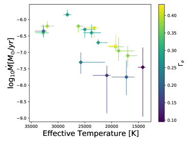
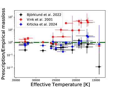
Figure 12: Derived mass-loss rates for our sample as function of effective temperature. The top plot shows the derived mass-loss rates and he colour shows the derived classical Eddington parameter for each star. The bottom plot shows the ratio between the theoretical prescriptions by Vink et al. (2001); Björklund et al. (2023); Krtička et al. (2024) and the empirically found values. The green line indicates where these are equal.

We next compare our empirically derived rates (figure 12) to the predictions by Vink et al. (2001), Krtička et al. (2024) and Björklund et al. (2023). As discussed in the introduction, the $\dot{M}(T_{\rm eff})$ behaviour for a fixed mass and luminosity differs between these prescriptions. In the context of the present study, the main difference in the predictions of these schemes is that Vink et al. (2001) predict significantly higher mass-loss rates for stars below $T_{\rm eff}\sim 22-25$ kK than for hotter stars, whereas Björklund et al. (2023) do not predict such a jump but instead a steady decrease of mass-loss rates with decreasing temperature. The Krtička et al. (2024) rates do not exhibit such a monotonic decrease of mass loss with decreasing temperature, but rather has a characteristic bump at $T_{\rm eff}\sim 13-15$ kK. This bump is very localised and predicts a rather modest mass loss increase (followed by a steep decrease), which also lies at the edge of our observational coverage range. As such, it is not possible to scrutinise this particular low-temperature feature in the mass-loss behaviour for the present set of stars (spectral types O8.5-B7).

The comparisons between Vink et al. (2001), Björklund et al. (2023), and Krtička et al. (2024) are shown in the bottom panel of Figure 12, where the ordinate displays predicted $\dot{M}$ divided by the empirical $\dot{M}$ derived in this paper, again plotted as function of effective temperature. All predicted rates have been computed by means of the ’mass-loss recipes’ provided in the corresponding papers, using the stellar parameters derived for each star ($L_{\star}$, spectroscopically derived $M_{\star}$, $T_{\rm eff}$, $\varv_{\infty}$), and a metallicity reflecting that of the LMC. Here we corrected for the higher solar metallicity used in Vink et al. (2001) compared to the Björklund et al. (2023) rates as described in Sundqvist et al. (2019). As such, additional dependencies on for instance $\Gamma_{\rm e}$ are naturally accounted for in these comparisons. At temperatures above $\sim 22.5$ kK all three prescriptions are, on average, fairly aligned with the empirical rates. However, at lower temperature the predictions by Vink et al. jump up as a result of the bistability jump causing their mass-loss recipe to over-predict the empirical rates by more than an order of magnitude. The recipe by Björklund et al. (2023) shows no such jump, and instead displays a rather constant trend with $T_{\rm eff}$, aligned with the trend inferred for the empirical rates. For the coolest star in our sample the Björklund et al. (2023) rates are much lower than our best-fit values. This might be an outlier or due to the extrapolation of the Björklund et al. (2023) model grid. For stars hotter than 26 kK, two stars agree very closely with the observation while two underestimate by about a factor 8. When comparing the observations to the Krtička et al. (2024) prescription we see that they also agree fairly well. However, in contrast to the Björklund et al. (2023) prescription the Krtička et al. (2024) prescriptions oscillate between over- and under-predictions.

Although the prescription by Björklund et al. (2023) reproduces the empirically found trend rather well, we observe from the bottom panel of figure 12 an almost constant underestimation with a relative offset of $\langle|\dot{M}_{\rm P}-\dot{M}_{\rm E}|/\dot{M}_{\rm E}\rangle\sim 0.5$ from our best-fit values, where $\dot{M}_{\rm P}$ denotes the prescription results and $\dot{M}_{\rm E}$ is the empirical mass-loss rate. This average is weighted with the error-margin. For the prescriptions by Vink et al. (2001) we split such average comparisons into stars with $T_{\rm eff}$ above and below the jump. For stars above this threshold we find $\langle|\dot{M}_{\rm P}-\dot{M}_{\rm E}|/\dot{M}_{\rm E}\rangle\sim 0.8$ and for stars below $\langle|\dot{M}_{\rm P}-\dot{M}_{\rm E}|/\dot{M}_{\rm E}\rangle\sim 20$. The Krtička et al. (2024) prescription fluctuates between over and under estimating but there is no clear cut-off temperature to split the prescription. If we compute the average relative offset for the full sample, we find $\langle|\dot{M}_{\rm P}-\dot{M}_{\rm E}|/\dot{M}_{\rm E}\rangle\sim 0.5$. Which is exactly the same as the Björklund et al. (2023) offset and close to the Vink et al. (2001) offset for the hot stars.

Again these comparisons and simple averages show quite clearly that the sudden increase in mass-loss rate predicted at the supposed bi-stability jump by the Vink et al. (2001) prescription is not present in these observational results.

We may further compare our results to other empirical studies. Bernini-Peron et al. (2023) show a study of 4 BSGs (B2-B5) in the Galaxy with access to UV spectra and therefore also try to constrain the clumping factor. The mass-loss rates acquired in that study are also higher for similar effective temperatures as expected due to the higher metallicity. They do find some localised increase when compared to 4 literature stars at hotter temperature, but this is hard to verify due to not covering the supposed bistability jump with the stars from their sample. In contrast Markova & Puls (2008) assume a smooth wind outflow and derive mass-loss rates for Galactic BSGs using H ${\alpha}$. Within our current spectroscopic formalism for wind clumping, these mass-loss values should be interpreted as upper limits. Assuming effects of clumping do not change the inferred rates of mass loss significantly across the region, we may still examine the mass-loss trend with effective temperature. Over their investigated temperature range the derived mass-loss rates decrease monotonically, showing no signs of an increase around 22.5 kK. The derived $\dot{M}$ in these Galactic stars are generally higher than those we infer here for LMC stars. As the luminosity ranges are comparable, this is due to the higher metallicity in the Milky Way. More recently, Rubio-Díez et al. (2022) examined winds of OB-stars, including 13 Galactic BSGs, by means of radio and far-infrared continuum observations. They derive values of $\dot{M}$ for the BSGs in their sample that are significantly higher than here. This is to be expected as, first, their measured mass-loss rate is an upper limit; second, they targeted very luminous objects, and, third, they consider a Galactic sample. Compared to this study, their general trend with effective temperature is similar. A comparison between their rates and the predicted Vink et al. (2001) rates therefore too shows a large discrepancy at temperatures below 22.5 kK, with the predictions higher than the empirical rates by between 1 and 2 orders of magnitude (for their estimates of maximum mass loss).

Very recently, de Burgos et al. (2024) used optical spectra of 116 Galactic BSGs in the temperature range 15 to 35 kK to derive upper limits to mass-loss rates (upper limits because they used smooth wind models); they did not find any signs of an upward trend in mass-loss rate with decreasing temperature in the predicted bistability region.

4.2 Terminal wind speeds

As can be seen in the top panel of figure 9, the resulting terminal wind speeds suggest a linear dependence on effective temperature. Fitting a linear function $\varv_{\infty}=aT_{\rm eff}-b$, we find best fit values $a=(9.7\pm 0.6)10^{-2}$km (sK)^-1 and $b=1360\pm 130$ km s^-1. As mentioned in the previous section, the linear behaviour as well as the numerical fit values are in line with the recent findings of Hawcroft et al. (2024b), who fitted $a=(8.5\pm 0.5)10^{-2}$ and $b=1150\pm 170$km s^-1 for their larger sample. Compared to the prescription from the modelling efforts by Vink & Sander (2021) we notice that the discontinuity at the supposed bi-stability range does not agree with the observed values. Instead we see a continues increase of $\varv_{\infty}$ with $T_{\rm eff}$. The classical study of UV P-Cygni lines by Lamers et al. (1995) found a sudden decrease in the ratio $\varv_{\infty}/\varv_{\rm esc}$ around $T_{\rm eff}\sim 21$ kK, a behaviour which has often been associated with the presence of a bistability jump, whereas other studies have found a more gradual decrease (e.g., Markova & Puls 2008). Here $\varv_{\rm esc}^{2}=2GM_{\star}(1-\Gamma_{\rm e})/R_{\star}$ is the effective (i.e., reduced by Thomson scattering) escape speed from the stellar surface. Figure 13 shows our measured $\varv_{\infty}/\varv_{\rm esc}$ against effective temperature. The figure is dominated by large scatter in the inferred values, reflecting also uncertainties in the stellar parameters used to compute $\varv_{\rm esc}$. We do indeed observe some indication of a downward trend in the range $T_{\rm eff}\sim 25-17$ kK, although also in our relatively small sample at least some outliers to this trend clearly exists on the cold end. Actually, one may detect a similar behaviour also in the above-mentioned larger study by Hawcroft et al. (2024b), if one zooms in on the region around $T_{\rm eff}\sim 20$ kK for LMC stars (see their Figure 5). However, in that study this quite subtle ’by-eye’ detected trend is statistically washed away by the large number of stars with hotter effective temperatures and the scarcity of stars with $T_{\rm eff}<20$ kK.

Nonetheless, although uncertainties are still large, there may be signs of the general trends observed by Crowther et al. (2006) present in this sample as well. This trend is similar to the trend by Lamers et al. (1995) but instead of a sudden downward jump upwards in $\varv_{\infty}/\varv_{\rm esc}$ a more gradual decrease with decreasing $T_{\rm eff}$ is seen instead.

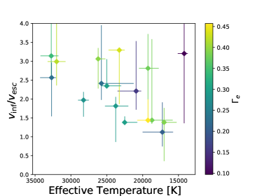
Figure 13: Terminal wind speed divided by escape speed plotted over temperature. The mass used to determine the escape speed is the effective spectral mass.

4.3 X-rays

Without X-ray ionisation the later-type stars in our sample show very little triple ionised carbon in their winds and outer atmospheres, resulting in absent or very weak C iv1550 lines, without any P-Cygni like wind signatures. Observations, in contract, show that some cooler stars in the sample have strong C iv1550 lines with clear wind signatures.To reproduce this, we added X-rays produced due to shocks in the wind also in this temperature region, as outlined in Sect. 2.2. To ensure all results are comparable even the stars that fit well without X-rays have been fitted with X-rays and those are the results noted here, with the exception of the coolest star in the sample for which the X-rays caused convergence issues. This also allows us to see if there is a noticeable improvement in fitting by including X-rays. Those hotter stars that do not need X-rays to excite carbon or the cool stars with no noticeable C iv give X-ray values with much higher error margins or very low values and the fit quality stays comparable.

Figure 14 shows the difference the X-rays make to the ability to fit the C iv and S iv wind resonance lines of sk$-70^{\circ}16$. The best-fit $\varv_{\infty}$ of the model including X-ray ionisation is 1000 km/s while the one without gives $\varv_{\infty}=500$ km/s. Notice how this big change in $\varv_{\infty}$ and the addition of X-rays as a whole did not influence the Si iv line noticeably while transforming the C iv line substantially, showing that the Si iv line is a poor indicator of $\varv_{\infty}$. Although introducing X-rays forces us to consider even more free input-parameters in our modeling, the upside of the addition is that it does not significantly affect any of the other parameters within our sample. For example, $T_{\rm eff}$ is typically slightly lowered when X-rays are included, but the reduction is always within the 1-$\sigma$ uncertainty of the originally found effective temperature. The issue is often that while weak, unsaturated UV resonance lines may still show clear signatures of line formation in the lower wind, they can be insensitive to $\varv_{\infty}$ due to very low optical depths in the outermost wind. To properly capture this one thus needs to model also the detailed wind ionisation balance, which is typically not done in the simplified large-scale approaches that work well on strong and (almost) saturated UV wind lines (e.g., Hawcroft et al. 2024b; Lamers et al. 1995).

We find an average $\log_{10}(L_{x}/L_{bol})=-7.3$ for our sample, however with very large error margins of $\pm 1$ to $\pm 2.5$. For individual stars the large errors cause the best fit range to reach down to $\log_{10}(L_{x}/L_{bol})<-8$. Our average value is on the same order as the often-quoted empirical relation $\log_{10}(L_{x}/L_{bol})=-7.2\pm 0.2$ found from X-ray observations of O-stars (Rauw et al. 2015). Crowther et al. (2022) have studied the X-ray properties of specifically O-stars in the LMC and found a similar relation $\log_{10}(L_{x}/L_{bol})=-6.90\pm 0.65$. It also agrees well with the X-ray luminosity range found by Bernini-Peron et al. (2023) ($\log_{10}(L_{x}/L_{bol})\approx[-7,-8.3]$). When computing the range of shock temperatures using equation 2, we note typical shock temperatures ranging from $10^{5}$ K, at the X-ray onset radius, to $5\times 10^{6}-10^{7}$ K at the terminal wind speed. Note again that the reasoning behind adding X-rays here was solely to reproduce the C iv1550 doublet in a few cooler stars but implemented in all for standardised comparison (see above). For the rest of the stars in our sample including X-rays does not improve the best fit quality. As such, the corresponding fit parameters become redundant and the uncertainties of X-ray luminosities extremely high.

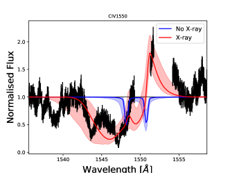
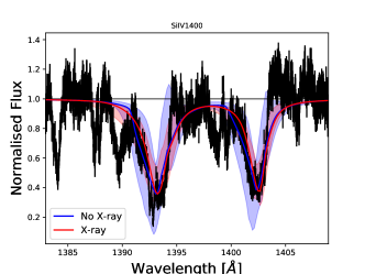
Figure 14: Three versions of the same doublet line per panel, in black we show the data from Sk$-70^{\circ}16$ a B2 II star in blue the best fit when not allowing for X-rays and in red the best fit when allowing for X-rays. The top panel shows the C iv 1550 line and the bottom panel shows the Si iv1400 line.

4.4 Clumping

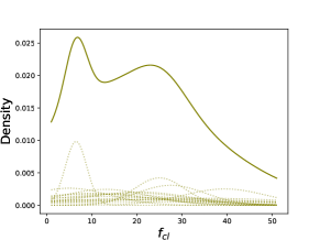
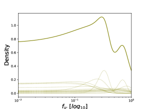
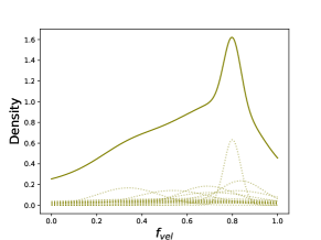
Figure 15: Approximate kernel distribution of the clumping parameters. In full lines we show the normalised approximate kernel distribution of the clumping parameter ($f_{\rm cl}$), the interclump density ($f_{\rm ic}$), and the velocity filling factor ($f_{\rm vel}$). In dashed lines the contributions of the separate fits contributing to the distribution.

Figure 10 shows that clumping is ubiquitous, however, the scatter and error margins of the clumping parameters are large, and our sample is rather small, making robust quantitative interpretations challenging. The Pearson correlation coefficient to find correlations between all clumping factors, the $\beta$ parameter, $T_{\rm eff}$, and mass-loss rate, showed no significant correlations for the clumping parameters with any of the other parameters. However, the aforementioned trends, such as the mass-loss rate, $T_{\rm eff}$ correlation and the $\varv_{\infty}$, $T_{\rm eff}$ correlation are reflected by the Pearson coefficient.

As by eye we perceived possible trends for the subsample of stars less than 30 kK, we did a similar test for those stars. However, this did not reveal significant trends in any of the combinations save for the ($f_{\rm cl}$, $T_{\rm eff}$) and ($f_{\rm cl}$, $\dot{M}$) relations. First off we see a tenuous increase in $f_{\rm cl}$ for decreasing $T_{\rm eff}$ . From line de-shadowing instability (LDI) simulations (Driessen et al. 2019) we expect a downward jump of $f_{\rm cl}$ as we go from O-stars to B-stars, but assuming our observed trend is real it could explain why this jump is difficult to observe. Although, we want to highlight again that this observed trend is rather tenuous. Because of the clear correlation between $\dot{M}$ and $T_{\rm eff}$, we also find a slightly stronger correlation between $f_{\rm cl}$ and $\dot{M}$. This is inline with the trends observed in O-stars by Brands et al. (2022), although they also highlight the delicate nature of this result.

Instead of correlations, we can study the general trends of the parameters not in respect to another. Figure 15 shows an approximate kernel distribution where each separate fit result is interpreted as a Gaussian with the uncertainty margin as the width of the Gaussian and each result is scaled by its $1/\chi^{2}$ value. Adding all these Gaussians together yields a distribution which is normalised to unity. This Gaussian allows us to talk about the behaviour of this parameter over the full sample when no clear trend is present. The clumping factor in our sample has a preference to around 20, but while for low clumping factors the likelihood stays strong, due to a single good fit, the tail towards the higher clumping factors decreases rapidly. The interclump density is less clearly peaked, but still has a visible peak around 0.4. The apparent long tail towards lower values also has to do with the displayed logarithmic axis, which visually prioritises small values and compresses the higher end of the axis. The velocity filling factor shows one of the possible pitfalls of this method, where one data point is dominating the distribution due to fitting well and having a low error-margin. The rest of the distribution is still useful, however, where we see a broad distribution with a relatively steep drop-off towards the lowest values.

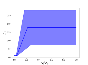
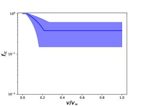
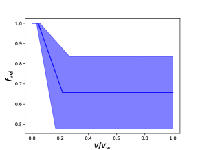
Figure 16: Change of the 3 clumping parameters as a function of $\varv/\varv_{\infty}$. The dark blue line shows the averages, with the blue shaded region showing the $1-\sigma$ region of these averages.

When taking a weighted average of the three clumping parameters we find: $\langle f_{\rm cl}\rangle=18\pm 10$, $\langle f_{\rm ic}\rangle=0.38\pm 0.23$ and, $\langle f_{\rm vel}\rangle=0.66\pm 0.18$. These values are representing the part of the wind where it is most structured; at low velocities (below the gas sound speed) the atmosphere is always assumed smooth. How the three clumping parameters on average change with velocity is shown in figure 16. The high mean value inferred for the interclump density sticks out, suggesting that we can expect that the interclump component comprises close to 40% of the average wind density. This is in stark contrast to alternative descriptions of wind clumping that are based on an effectively void interclump component. Non-zero $f_{\rm ic}$ have also been found in the previous studies (of O-stars) by H21 and B22. These best fits, although quite a bit lower to the value quoted here (H21 $f_{\rm ic}=0.13\pm 0.08$, B22 $f_{\rm ic}=0.13_{-0.13}^{+0.15}$), seem at least not-pointing towards zero. As further discussed in the next section, this changes significantly the interpretation of the clumping parameters in terms of the relations between clumping factors, clump over-densities, and volume filling factors, and also invalidates the commonly applied assumption that the complete wind mass is compressed into dense and small clumps.

The inferred mean value of the (maximum) clumping factor is higher than in models by Driessen et al. (2019) and also higher than the Galactic observational study by Bernini-Peron et al. (2023) where they find clumping factors of at most 2. We do note that both the fitting method and clumping description in their empirical study are different to ours, but the large difference is still noteworthy. Our derived clumping factors are, in contrast, lower than the sample averages for Galactic O-supergiants by H21 ($f_{\rm cl}\approx 25$) and for LMC O and WNh stars by B22 ($f_{\rm cl}\approx 29\pm 15$) who use the same clumping model. A downward trend with $T_{\rm eff}$ would be consistent with the linear analysis and non-linear instability simulations by Driessen et al. (2019), but establishing such a potential trend empirically would require a (significantly) larger sample than investigated here. In view of these empirical uncertainties and the fact that the theoretical clumping-study by Driessen et al. (2019) only used 1D simulations neglecting the influence of a turbulent stellar surface (Jiang et al. 2015; Debnath et al. 2024) on the clumpy outflow, it is at this point not meaningful to discuss more quantitative comparisons of empirical and theoretical clumping factors in this regime.

The empirical data suggest that clumping on average starts at low wind velocities within our sample, with several of the $1\sigma$ error ranges extending down towards our lower allowed bound at $\varv\approx a$. While this is qualitatively consistent with previous empirical studies for hotter O-stars (Puls et al. 2006; Cohen et al. 2011; Hawcroft et al. 2021; Brands et al. 2022), corresponding 1D instability simulations (Sundqvist & Owocki 2013), and 3D radiation transfer studies (Šurlan et al. 2013) also here we caution against more quantitative interpretations due to the fact that current wind clumping implementations may not be ideally suited for turbulent layers near the photosphere (see discussion in Debnath et al. 2024).

Finally, the fits for the velocity filling factor suggest that velocity-porosity effects indeed play a role in the spectrum formation of these winds, with a mean value that seems reasonable in view of general theoretical expectations (see discussion in Sundqvist & Puls 2018). The scatter is high, however, and no significant trends can be identified from the present data sample. We note in this context that there exists an independent observational indication for velocity-porosity (parametrised in the present study by a velocity filling factor) in BSG winds, namely via direct comparison of the depth of the blue and red absorption dips of unsaturated UV resonance doublets (Prinja & Massa 2013). Parsons et al. (2024) investigated this for stars in the ULLYSES sample and found similarly that there are clear indications for velocity-porosity across the sample but no significant trend with temperature. They also find very large scatter in their inferred optical depth ratios, as well as a strong temporal variation. Such temporal variations are not taken into account here as we combine two observations (UV+OPT) not taken simultaneously.

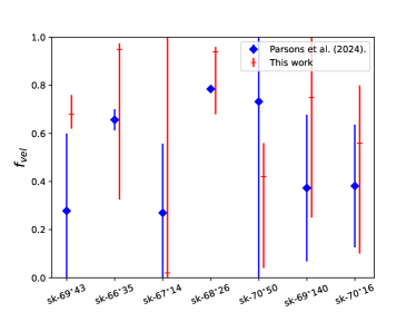
Figure 20: Velocity filling factor in this study compared to Parsons et al. (2024). This figure shows a comparison between the velocity filling factor we derived here, and the velocity filling factor from Parsons et al. (2024). We compute the velocity filling factor from optical depths of the red and blue absorption dips obtained by Parsons et al. (2024) using equation 23 from Sundqvist et al. (2014). When the ratio of the red and blue absorption dips reached values above 2 we excluded it here as this results in non-physical $f_{\rm vel}$.

Comparing the obtained optical depths from Parsons et al. (2024) to the velocity filling factors derived here quantitatively is challenging, but equation 23 from Sundqvist et al. (2014) does allow us to approximate the vorosity factor ($f_{\rm vor}$) from the optical depth of the blue and red absorption dips. This $f_{\rm vor}$ is then related to $f_{\rm vel}$ by equation 14 in Sundqvist & Puls (2018). The empirically derived blue and red optical depths from Parsons et al. (2024) then provides an independent estimate of $f_{\rm vel}$, which can be directly compared to the values derived in this paper. The key qualitative point from this analysis is that velocity-porosity clearly is required in order to explain the blue to red optical depth ratios measured by Parsons et al. (2024). However, due to high uncertainties in these measured ratios, we still find significant quantitative error margins in $f_{\rm vel}$ (see Fig. 20). Nonetheless, within these (admittedly very large) error margins, the two methods seem to provide results that overall are in reasonable agreement. This lends some support to the ability of the fast method utilised by Parsons et al. (2024) for identifying stars where velocity-porosity is important in their UV resonance wind line formation.

4.5 On the interpretation and validity of current wind clumping methods for spectroscopic studies

The generally high values found for the interclump density challenge some common assumptions and interpretations regarding wind clumping in massive stars. Namely, in most previous studies it has been assumed that the interclump medium is effectively void, so that all wind mass is contained within clumps and the relation between the clumping factor and clump volume filling factor $f_{\rm vol}$ is simply $f_{\rm cl}=f_{\rm vol}^{-1}$, accompanied by a characteristic clump over-density $D=\rho_{\rm cl}/\langle\rho\rangle=f_{\rm cl}$. But for the typical values of $f_{\rm ic}\equiv\rho_{\rm ic}/\langle\rho\rangle$ found here, these simple relations no longer hold. Instead we must use the full relations for the stochastic two-component medium (Sundqvist & Puls 2018):

$$f_{\rm vol}=\frac{(f_{\rm ic}-1)^{2}}{f_{\rm cl}+f_{\rm ic}^{2}-2f_{\rm ic}}$$ (10)

$$D=\frac{\rho_{\rm cl}}{\langle\rho\rangle}=\frac{1-f_{\rm ic}(1-f_{\rm vol})}{f_{\rm vol}}$$ (11)

for a mean wind density

$$\langle\rho\rangle=f_{\rm vol}\rho_{\rm cl}+(1-f_{\rm vol})\rho_{\rm ic}$$ (12)

and clumping factor

$$f_{\rm cl}\equiv\frac{\langle\rho^{2}\rangle}{\langle\rho\rangle^{2}}=\frac{f_{\rm vol}\rho_{\rm cl}^{2}+(1-f_{\rm vol})\rho_{\rm ic}^{2}}{(f_{\rm vol}\rho_{\rm cl}+(1-f_{\rm vol})\rho_{\rm ic})^{2}}.$$ (13)

Let us first point out that while the above involves the quantities $f_{\rm vol}$, $f_{\rm cl}$, $f_{\rm ic}$, and $D$, only two of these are independent. This is readily seen from the equation for mean density, which we may write in normalised form $1=f_{\rm vol}D+(1-f_{\rm vol})f_{\rm ic}$. Thus, if one chooses to set, say, $f_{\rm ic}$ and $D$, $f_{\rm vol}$ follows accordingly, and thereby also $f_{\rm cl}$ from the relations above. That is, while in our modeling we choose the input parameters $f_{\rm cl}$ and $f_{\rm ic}$ we may as well have chosen any pair of the above four quantities and then calculated out the others. Similarly, in the previously standard method of simply assuming $f_{\rm ic}=0$, only one of the above parameters is necessary to set; e.g. for an input $f_{\rm vol}$ we see directly that indeed $f_{\rm vol}^{-1}=D=f_{\rm cl}$.

To illustrate the situation when $f_{\rm ic}\neq 0$, we take our derived best-fit values for star Sk$-67^{\circ}14$; $f_{\rm ic}=0.86$ and $f_{\rm cl}=8.0$. This yields a clump volume filling factor $f_{\rm vol}=0.003$ that is now much lower than $f_{\rm cl}^{-1}=0.13$. Similarly we find for the characteristic clump over-density $D=51$, whereas interpreting this the standard way would yield $D=f_{\rm cl}=8$. Moreover, identifying mass-contributions from the clumps and the interclump medium from the equation for $\langle\rho\rangle$ one gets for the former $Df_{\rm vol}=0.15$ and the latter $(1-f_{\rm vol})f_{\rm ic}=0.85$; that is, we find here that most of the wind mass is actually not contained in the dense clumps, but rather in the interclump medium. Although this star lies on the extreme end of our sample, similar re-interpretations are necessary also when taking the weighted averages of our sample $f_{\rm cl}=18\pm 10$ and $f_{\rm ic}=0.38\pm 0.23$, whereby we obtain $f_{\rm vol}=0.022\pm 0.020$ (vs. $f_{\rm cl}^{-1}=0.06\pm 0.03$), $D=28\pm 27$ (vs. $f_{\rm cl}=18\pm 10$) and that the interclump medium contributes $37\pm 22$% of the wind mass. These general tendencies arise because we typically find a significant interclump density together with a rather high rms over-density $\sqrt{\langle\rho^{2}\rangle}/\langle\rho\rangle$ from the observational data. This combination forces clumps to be confined into very small volumes, so that relative contributions from the clump and interclump media to the total wind mass become approximately $1-f_{\rm ic}$ and $f_{\rm ic}$, respectively. Additionally, since typically $f_{\rm vel}$ is significantly higher than $f_{\rm vol}$, it means that these spatially very confined clumps within our formalism are quite spread out in velocity space.

H21 find values $f_{\rm ic}\sim 0.15-0.3$ from their sample of Galactic O-supergiants. B22 split their sample of O and WNh stars into two categories according to stellar luminosity, and find sample averages for their low and high luminosity stars $f_{\rm ic}=0.07\pm 0.06$ and $f_{\rm ic}=0.28\pm 0.21$, respectively. Our sample average here is thus noticeably higher, but still in overall qualitative agreement with these previous results for high luminosity O-stars regarding the possibility of a significant non-clump wind mass (we note in this respect that, originally, the discussion in Sundqvist & Puls 2018, based largely on 1D simulations, argued for low ”standard” values on order $\sim$0.01-0.2 for this parameter). The increase of $f_{\rm ic}$ in our study compared to H21 and B22 could be due to the different temperature region or due to slight differences in the fitting routine such as different fitting assumptions. On the other hand, in an independent study Šurlan et al. (2013) used 3D Monte-Carlo radiation transfer, in combination with the 1D code PoWR, for a Galactic O-star analysis and showed that the inclusion of interclump density was needed to reproduce the P v 1118 doublet. They got best correspondence for relatively high interclump density ($0.1-0.4<\rho>$), however including the interclump density reduced the effect of the clumping factor on the line profiles. These counteracting effects probably also increase the error-margin of our clumping parameters, but due to the global fits of the GA method such inter-dependencies are all taken into account.

Overall, the general picture that emerges is different from that which has been assumed in spectroscopic studies of massive-star wind clumping previously; a significant fraction of the wind mass seems actually not to be contained in small-scale clumps, but rather in the medium in between these. While this is in stark contrast with the assumptions underlying the vast majority of previous spectroscopic studies, it actually correlates rather well with recent theoretical results from multi-dimensional radiation-hydrodynamic simulations. The 3D models of Wolf-Rayet stars by Moens et al. (2022) indeed find that approximately half of the wind mass is contained in parcels having densities lower than the mean density of the wind, illustrating again the general issue with assuming a wind completely dominated by dense clumps.

However, in these recent simulations it is also found that the density distributions do not resemble a two-component medium, but rather have Gaussian-like distributions (likely log-normal ones, see Owocki & Sundqvist 2018 and Schultz et al. 2020) where the most probable density is quite close to the mean and the dispersion is large. Since similar results are suggested also by the 2D O-star simulations by Debnath et al. (2024) and Driessen (2022), the latter including effects of the (LDI, Owocki & Rybicki 1984) (see their Fig. 8.3), this may indicate issues also with the generic assumption applied here of an effective two-component medium consisting of clumps and an interclump medium. Additionally, the models by Jiang et al. (2018) and Debnath et al. (2024) that consider deep sub-surface layers clearly indicate that also the photosphere is very variable and structured, whereas in the clumping description applied here we assume an inner boundary for possible structure formation at the wind sonic point (see Fig. 16). In this respect, we note further that (as mentioned in Sect. 2) in our current approach the ionisation balance is only derived for an effective medium, and thus not for the interclump and clumped components separately. Overall, in view of these results a general re-calibration of methods used to account for wind clumping effects in spectroscopic studies may thus be needed (see Owocki & Sundqvist 2018 for a first attempt that focuses on transfer effects arising from the turbulent density structures typically seen in multi-D simulations of hot star winds).

5 Summary and outlook

We have analysed the optical X-shooter and UV ULLYSES spectra of 15 OB supergiants in the LMC using model atmosphere code fastwind and the GA fitting approach Kiwi-GA, resulting in 18 consistently determined stellar (7) stellar and (11) wind parameters. Derived spectroscopic masses in our sample range from 15-75 $M_{\odot}$ and effective temperatures lie in the range 35-14kK with uncertainty margins of around $\pm 1500$K per star. Our sample of stars have been selected with the goal to determine if the so-called bistability jump, an upward jump in mass loss towards cooler photospheres within the observed temperature regime, is observable when the parameter degeneracy of wind clumping is broken by the availability of UV data. As such, we focused especially on determining accurate mass-loss rates. Our derived rates range from $-7.7$ to -6 $\log_{10}(M_{\odot}/$yr), taking into account inhomogeneities of the wind in the most detailed way current 1D atmosphere codes allow.

By determining the mass-loss rates of all stars within $\pm 0.3$ dex for most of them, we can see that no sudden mass loss increase in this effective temperature regime is present in the empirical analyses. From comparisons to different theoretical predictions we see that the jump described by Vink et al. (2001) (which is the current standard recipe to include in applications like stellar evolution modelling) is drastically overestimating the mass-loss rates on the cool side of their predicted jump. For our sample we derive, similarly to how we derive the uncertainty margins on the cumulative clumping parameters in figure 15, an overestimation by about a factor $\sim 24$. By contrast, on the hotter side of the predicted jump these same predictions are typically rather well aligned with the empirically derived rates, on average the offset is $\sim 0.8$ times the empirically derived rates. Comparing to the alternative theoretical rates by Björklund et al. (2023), which decreases monotonically with temperature and thus do not find any mass loss jump (see discussions in previous sections). We notice that the trend with $T_{\rm eff}$ of these predictions is rather well aligned with the empirical data, showing a relatively constant underestimation and an offset of $\sim 0.5$ times the empirically derived rates. If a jump were present in the observed sample it would not be possible to find such a constant offset with a prescription that is only decreasing with decreasing $T_{\rm eff}$. Note that for the computation of these ratios we did not take into account the uncertainty margins of the prescriptions, which are always present as they are, on purpose, simple fits of a grid of models resulting in some scatter between the fits and the actual model results; as such, the quoted error-margins are likely to be slightly underestimated. The Krtička et al. (2024) prescriptions further also align overall well with the observed mass-loss rates, but our current data-set is not optimal to test the weaker mass-loss bump present at cooler temperatures, as it is also very localised( decreasing aggressively when moving toward even cooler temperatures, see Fig. 1). As such we can here neither confirm nor exclude a presence of the modest bump seen in the models by Krtička et al. (2024). The localised behaviour in temperature and comparatively weaker strength of the bump would make this feature relatively hard to verify in general, but impossible with our sample due to its temperature position.

Our derived terminal wind speeds are very much in line with the findings of Hawcroft et al. (2024b). The terminal wind speeds show a very linear dependence on the effective temperature even when masses and luminosities vary heavily. When trying to derive $\varv_{\infty}$ from the C iv1550 doublet, which typically is the main diagnostic for terminal wind speeds, we noticed that stars which have optical spectra that point clearly towards cool B stars sometimes still had strong C iv lines, although they are too cool to ionise a sufficient amount of carbon atoms to C iv in order to have strong C iv lines. To solve this we included ionisation due to additional X-rays in the wind also for stars down to $T_{\rm eff}\approx 15$ kK. This produced a sufficient amount of C iv atoms to model the C iv1550 doublet, whereas, interestingly enough, it did neither change the Si iv wind lines nor have a noticeable change on other fit parameters such as mass loss or clumping parameters. Such effects from X-ray ionisation for BSGs mimic the well known so-called wind ’super-ionisation’ for O-stars (often discussed in the context of OVI, Cassinelli & Olson 1979; Macfarlane et al. 1994; Krtička & Kubát 2009). However, even in B-stars this effect has been noted although less commonly mentioned (Macfarlane et al. 1994).

We derived constraints on a collection of clumping parameters which describe inhomogeneities in the wind ($f_{\rm cl},f_{\rm ic},f_{\rm vcl,start},f_{\rm vcl,max},f_{\rm vel}$). For $f_{\rm cl}$ we obtained a sample average $18\pm 10$, where the large error margin primarily is due to the large spread of best-fit clumping factors. Perhaps most strikingly in our empirical study of wind clumping are the high values of $f_{\rm ic}$. Here we obtain a sample average $0.38\pm 0.23$, where again the large uncertainty primarily is due to the large spread of the best-fit values; indeed, for individual stars we find values up to $0.92_{-0.22}^{+0.02}$. These high interclump densities may be viewed as surprising in the sense that a widely used assumption in 1D atmospheric and spectroscopic modelling has been that all wind mass is contained in the clumps; by contrast, here we find that typically about half of the wind mass is actually within the interclump regions. On the other hand, in view of recent multi-dimensional radiation-hydrodynamical simulations of hot star atmospheres with winds (Moens et al. 2022; Debnath et al. 2024) this may not be so surprising after all, since these tend to display Gaussian-like density distributions centred quite close to the mean rather than bimodal distributions with dominant over-dense clumps (which had been the prevailing thought based largely on 1D LDI simulations, e.g., Sundqvist & Owocki 2013; Driessen et al. 2019). In the simulations by Moens et al. (2022) the accumulative density distributions indeed show that almost half of the wind mass is contained in parcels that have densities lower than the mean density of the wind. Since similar results seem to be indicated also by multi-D simulations including the LDI (Driessen 2022), but has yet to be further quantified, our results here indicate a need to rethink how the radiation-driven wind is described in 1D codes used for spectroscopic modelling, also as this very basic assumption greatly influences not only the density structure of the wind but also its ionisation structure.

An interesting follow up to these results will be the study of similar objects in the SMC, for which we have equivalent data thanks to the ULLYSES program (Roman-Duval et al. 2020) and the X-Shooting ULLYSES (Vink et al. 2023; Sana et al. 2024). The goal will be to find if these empirical mass loss and clumping trends continue to lower metallicity. Additionally, with very comparable methodology for SMC and LMC samples it should be possible to also study the mass-loss behaviour scaling with metallicity. To this end we would be able to compare to other SMC studies on the same data in other temperature regimes (Parsons et al. 2024; Backs et al. 2024; Bernini-Peron et al. 2024) and other LMC samples studying the O-star regime (Brands et al. 2022; Hawcroft et al. 2024a) (Brands et al. (in prep.)) and comparing to studies in the Milky Way (Hawcroft et al. 2021; Bernini-Peron et al. 2023; de Burgos et al. 2024). A first look at how the sample range can easily be expanded by studies using similar fitting routines and methodology is shown in figure 17. Brands et al. (in prep.) studied O-stars in the LMC and therefore complements our sample to the hotter side. Figure 17 shows our sample again but the thinner crosses show the mass-loss rates and effective temperatures of the study by Brands et al. (in prep.). We can see that the trend of increasing mass-loss rates with increasing temperatures and $\Gamma_{e}$ is still present in this larger sample. As expected the error margins in this high temperature regime are smaller, as we already saw in our sample, where the hotter stars have lower error in mass-loss rate. Object sk$-68^{\circ}155$ is present in both samples and have very comparable fit-parameters in both studies (with the exception of the carbon abundance).

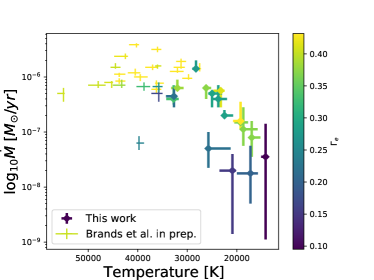
Figure 17: Expanding the present sample with study by Brands et al. (in prep.).

Finally, another interesting step would be to further study the effects of not including a strong bistability jump in evolution calculations. The lack of a prominent jump in observations means that stellar evolution codes currently being used as standards to describe single massive star evolution are also likely to significantly overestimate the loss of mass and angular momentum in this temperature and luminosity regime, perhaps then even influencing the viability of single stripped star formation (see, e.g., discussion in Björklund et al. 2023) or changing surface abundances (Josiek et al. 2024), and rotation Keszthelyi et al. (2017); Britavskiy et al. (2024). However, in this respect we note that for even higher luminosity to mass ratios than those examined in this paper, multi-dimensional models in this temperature regime suggest that strong winds can be ignited already from hot and optically thick sub-surface layers (Jiang et al. 2018), which may enhance mass-loss rates beyond the standard luminosity scalings of the stars with line-driven winds studied in this paper. And indeed, empirically this then approaches the region where we find the so-called Luminous Blue Variables (LBVs), for which it is well known that they undergo vigorous and variable mass loss (see overview in Vink 2022). We would argue that it should be a key focus for future (both empirical and theoretical) studies to try and better constrain the mass loss properties of this (very) high-luminosity region in the HR diagram.

Data availability

The fits of all stars discussed here and the distribution of the GA models are available at https://zenodo.org/records/13948998

Appendix A Remarks on the results

The goal of this paper was not to focus on the CNO abundances in particular. However, as they are needed fit parameters to derive the other parameters we shall briefly highlight what we can learn from them. The CNO abundance as a whole is expected to stay constant during the evolution of the star as one element gets converted into the other. To this effect to check the validity of our CNO abundances we have made figure 18 showing the sum of CNO massfractions and propagating the uncertainties for each of them. As expected, the sum of CNO abundances with the uncertainty stays close to the base sum.

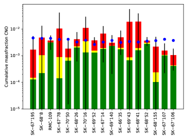
Figure 18: Cumulative CNO mass fraction; Here the CNO abundance is plotted for each star, (C in green, N in yellow, and O in red) in the sample with in black-lines the uncertainty on the sum of the CNO abundance. The blue dots indicates the expected cumulative CNO massfraction from Vink et al. (2023)

Appendix B Line list

3]

Table 5: Short caption of Table A.3.

Def	mol	Ion	$\lambda$	$\chi$	$\log gf$	N	e	rad	$\delta$	$\delta$ red	References
A	CH	1	3638	0.002	$-$2.551				$-$150	150	Jorgensen et al. (1996)

Table 5: continued

Table 6: Detailed list of all spectral lines which are fitted.

Ion	Wavelength $[\AA]$	Line window
C iv	1168.9, 1169.0	C iv 1196b
C iii	1174.9, 1175.3, 1175.6	C iv 1169b
	1175.7, 1176.0, 1176.4
Si iv	1393.8, 1402.8	Si iv 1400
C iv	1548.2, 1550.8	C iv 1550
O iii	3961.6	H$\epsilon$
He i	3964.7	H$\epsilon$
H i	3970.1	H$\epsilon$
He ii	4025.4	He i 4026
He i	4026.2	He i 4026
C iii	4068.9, 4070.3	C iii 4070
O ii	4069.6, 4069.9,	C iii 4070
	4072.16, 4075.86
S iv	4088.9, 4116.1	H$\delta$
N iii	4097.4, 4103.4	H$\delta$
H i	4101.7	H$\delta$
Si ii	4128.1, 4130.9	Si ii 4128
N iii	4195.8, 4200.1, 4215.77	He ii 4200
He ii	4199.6	He ii 4200
C ii	4267.0, 4267.3	C ii 4267
He ii	4338.7	H$\gamma$
H i	4340.5	H$\gamma$
O ii	4317.1,4319.6, 4366.9	H$\gamma$
N iii	4345.7, 4332.91	H$\gamma$
N iii	4379.0, 4379.2	He i 4387
He i	4387.9	HeI4387
O ii	4414.9, 4417.0	O ii 4416
He i	4471.5	He i 4471
N ii	4613.9, 4621.4, 4630.5	N ii 4601
	4601.5, 4607.2, 4643.1
N iii	4534.6	He ii 4541
He ii	4541.4	He ii 4541
Si iii	4552.6, 4567.8, 4574.8	Si iii 4552
C iii	4647.4, 4650.2, 4651.5	C iii N iii COLD/HOT
N iii	4634.1, 4640.6, 4641.9	C iii N iii COLD/HOT
O ii	4638.9, 4641.8,	C iii N iii COLD
	4661.6, 4676.2
He ii	4685.6	He ii 4686
N iii	4858.7, 4859.0, 4861.3,	H$\beta$
	4867.1, 4867.2, 4873.6
He ii	4859.1	H$\beta$
H i	4861.4	H$\beta$
He i	4921.9	He i 4922
He ii	5411.3	He ii 5411
O iii	5592.3	O iii 5592
C iii	5695.9	C iii 5695
He i	5875.6	He i 5875
He ii	6527.1	He ii 6527
He ii	6559.8	H ${\alpha}$
H i	6562.8	H ${\alpha}$
C ii	6578.1, 6582.9	C ii 6578
He i	6678.2	He ii 6683
He ii	6682.8	He ii 6683
He i	7065.2	He i 7065

• Note: The first column shows the atom and its ionisation stage which is responsible for the transition. The second column shows the corresponding wavelength with possible multiplets. The third column shows where to find this line in the fit summary which is available on Zenodo.

Appendix C Fit summaries

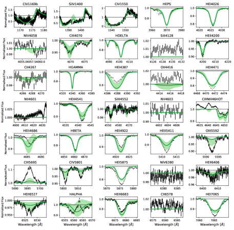
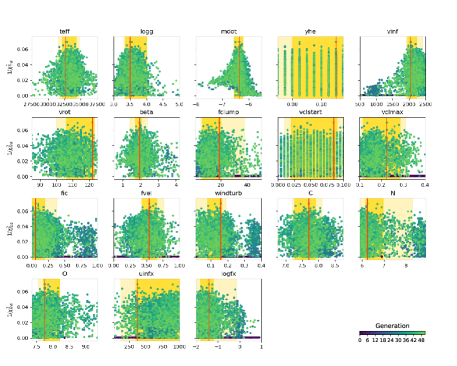
Figure 21: Fit summary of object Sk$-67^{\circ}106$. The top of this figure shows the fitted line windows with in solid green line the best model fit and in the light green area the $1-\sigma$ uncertainty area of the fit. The data is shown in black. In the bottom part we show the resulting probability distribution of these fits in the top. Each model produced while running the GA is one dot in this plot with the colour showing the generation of the model. The better the model fits the higher the $1/\chi^{2}_{\rm red}$. The best model is noted by the red line and the 1 and 2 $\sigma$ uncertainties are highlighted by the yellow regions.

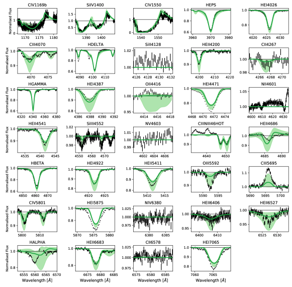
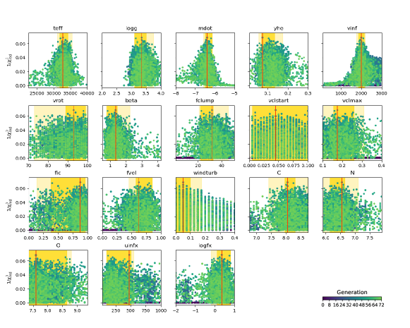
Figure 22: Same as figure 21 but for object Sk$-67^{\circ}107$.

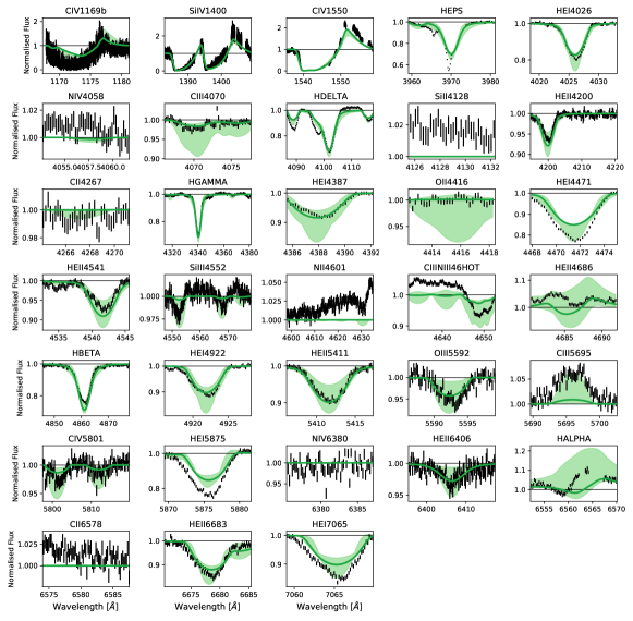
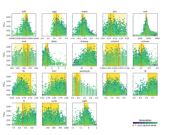
Figure 23: Same as figure 21 but for object Sk$-68^{\circ}155$.

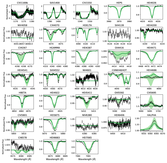
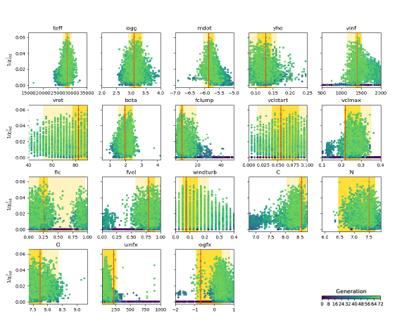
Figure 24: Same as figure 21 but for object Sk$-68^{\circ}52$.

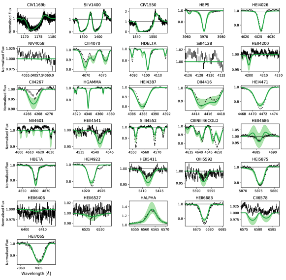
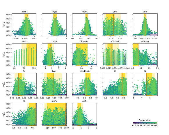
Figure 25: Same as figure 21 but for object Sk$-68^{\circ}41$.

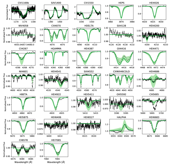
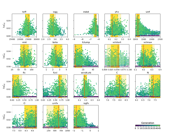
Figure 26: Same as figure 21 but for object Sk$-69^{\circ}43$.

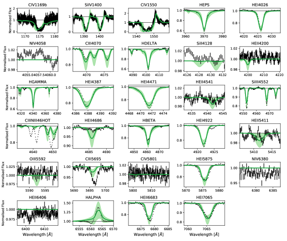
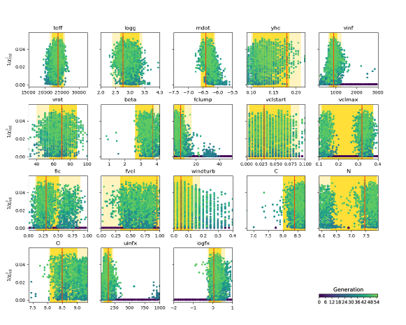
Figure 27: Same as figure 21 but for object Sk$-66^{\circ}35$.

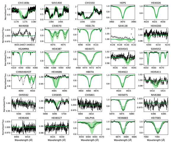
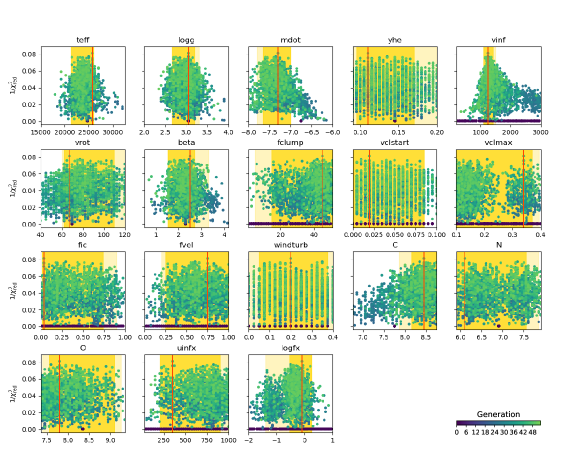
Figure 28: Same as figure 21 but for object Sk-$69^{\circ}140$.

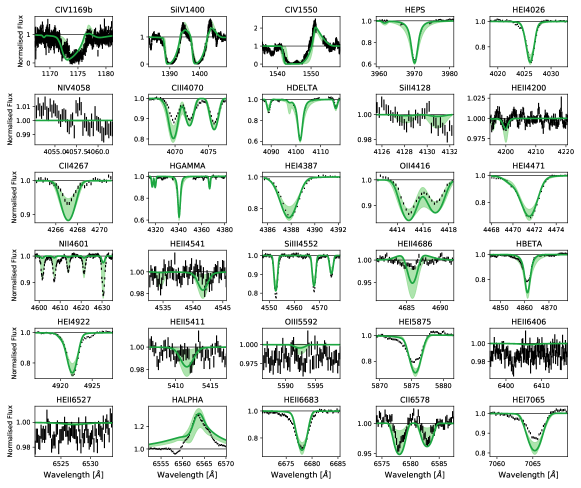
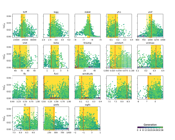
Figure 29: Same as figure 21 but for object Sk$-67^{\circ}14$.

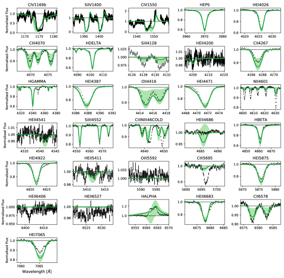
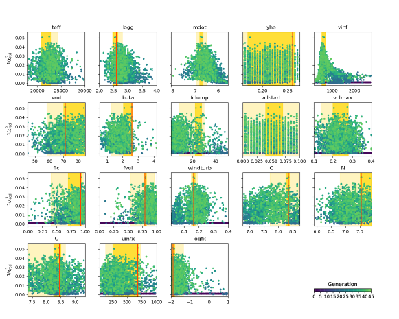
Figure 30: Same as figure 21 but for object Sk$-69^{\circ}52$.

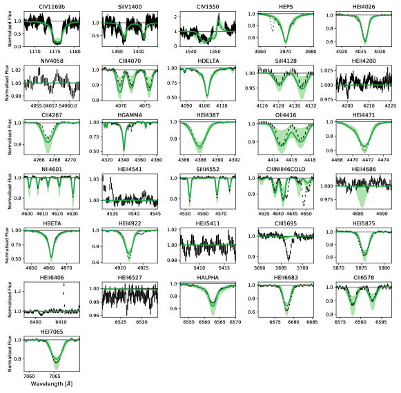
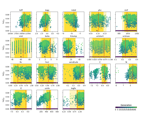
Figure 31: Same as figure 21 but for object Sk$-70^{\circ}16$.

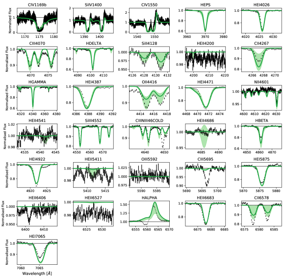
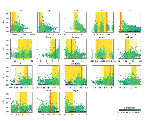
Figure 32: Same as figure 21 but for object Sk$-68^{\circ}26$.

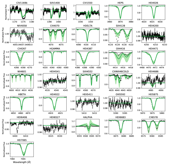
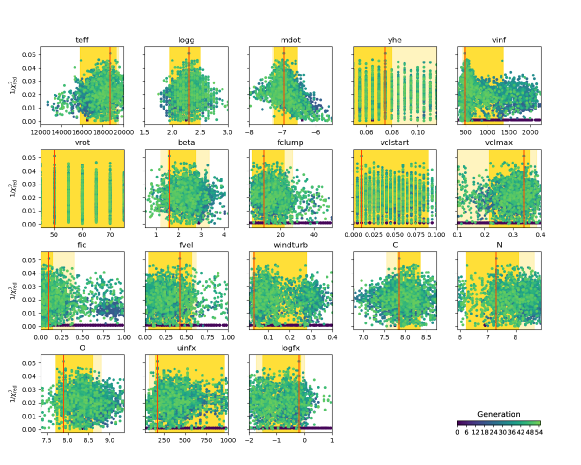
Figure 33: Same as figure 21 but for object Sk$70^{\circ}50$.

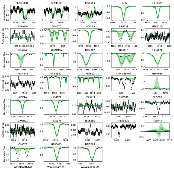
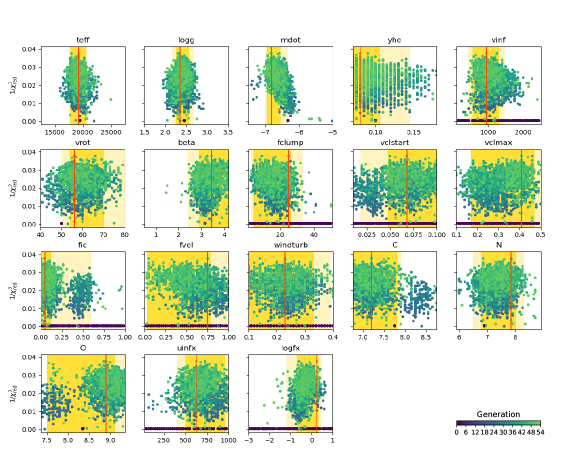
Figure 34: Same as figure 21 but for object Sk$-67^{\circ}78$.

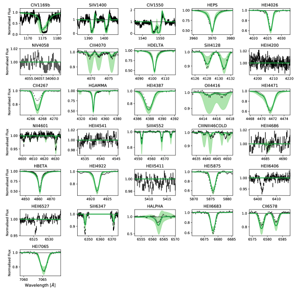
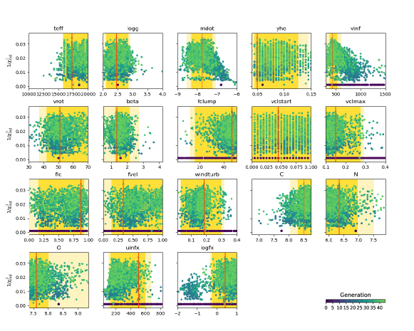
Figure 35: Same as figure 21 but for object RMC-109.

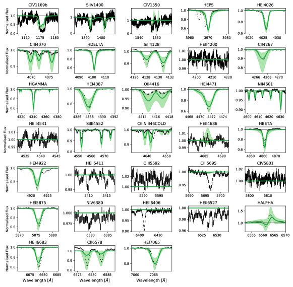
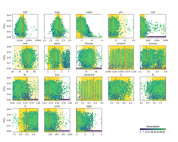
Figure 36: Same as figure 21 but for object Sk$-68^{\circ}8$.