Adversarial Score Identity Distillation: Rapidly Surpassing the Teacher in One Step

Abstract

Score identity Distillation (SiD) is a data-free method that has achieved state-of-the-art performance in image generation by leveraging only a pretrained diffusion model, without requiring any training data. However, the ultimate performance of SiD is constrained by the accuracy with which the pretrained model captures the true data scores at different stages of the diffusion process. In this paper, we introduce SiDA (SiD with Adversarial Loss), which not only enhances generation quality but also improves distillation efficiency by incorporating real images and adversarial loss. SiDA utilizes the encoder from the generator’s score network as a discriminator, boosting its ability to distinguish between real images and those generated by SiD. The adversarial loss is batch-normalized within each GPU and then combined with the original SiD loss. This integration effectively incorporates the average “fakeness” per GPU batch into the pixel-based SiD loss, enabling SiDA to distill a single-step generator either from scratch or by fine-tuning an existing one. SiDA converges significantly faster than its predecessor when trained from scratch, and swiftly improves upon the original model’s performance after an initial warmup period during fine-tuning from a pre-distilled SiD generator. This one-step adversarial distillation method establishes new benchmarks in generation performance when distilling EDM diffusion models pretrained on CIFAR-10 (32x32) and ImageNet (64x64), achieving FID scores of 1.499 on CIFAR-10 unconditional, 1.396 on CIFAR-10 conditional, and 1.110 on ImageNet 64x64. It sets record-low FID scores when distilling EDM2 models trained on ImageNet (512x512), surpassing even the largest teacher model, EDM2-XXL, which had an FID of 1.81 with classifier-free guidance. Our SiDA’s results—achieved without classifier-free guidance—record FID scores of 2.156 for EDM2-XS, 1.669 for EDM2-S, 1.488 for EDM2-M, and 1.465 for EDM2-L, demonstrating significant improvements across all model sizes. Our open-source code will be integrated into the SiD codebase.

1 Introduction

Modeling the distribution of high-dimensional data, such as natural images, has been a persistent challenge in machine learning (Bishop, 2006; Murphy, 2012; Goodfellow et al., 2016). Before the emergence of deep generative models, research focused primarily on constructing hierarchical models constrained by parametric distributions (Blei et al., 2003; Griffiths & Ghahramani, 2005; Fei-Fei & Perona, 2005; Chong et al., 2009; Zhou et al., 2009) and developing neural networks with stochastic binary hidden layers (Hinton et al., 2006; Salakhutdinov & Hinton, 2009; Vincent et al., 2010), supported by robust inference techniques such as Gibbs sampling, maximum likelihood, variational inference (Hoffman et al., 2013; Blei & Jordan, 2006), and contrastive divergence (Hinton, 2002).

The last decade has witnessed significant advancements in deep generative models, including generative adversarial networks (GANs) (Goodfellow et al., 2014; Reed et al., 2016; Karras et al., 2019), normalizing flows (Papamakarios et al., 2019), and variational auto-encoders (VAEs) (Kingma & Welling, 2014; Rezende et al., 2014). Although VAEs are noted for their stability, they often produce blurred images, while GANs are acclaimed for their ability to generate photorealistic images despite challenges with training instability and generation diversity. These dynamics have driven research towards refining statistical distances to more accurately measure discrepancies between true and generated data distributions, especially in scenarios where traditional metrics fail due to non-overlapping supports in high-dimensional spaces (Arjovsky et al., 2017; Li et al., 2017; Zheng & Zhou, 2021).

Diffusion models (Sohl-Dickstein et al., 2015; Song & Ermon, 2019; Ho et al., 2020; Karras et al., 2022) have further revolutionized this field with their ability to produce photorealistic images, albeit with multiple iterative refinement resulting in slow sampling speeds. In response, significant efforts have been directed towards developing efficient methods to utilize pretrained diffusion models for reversing the forward diffusion process through iterative refinement.

Departing from conventional methods, Diffusion-GAN (Wang et al., 2023b) reframes forward diffusion as a cost-effective, domain-agnostic data-augmentation strategy to tackle issues of non-overlapping distribution support. This approach introduces noise at various levels and utilizes statistical distances such as Jensen-Shannon divergence (JSD) for comparing distributions. The method promotes alignment between the true and generated data distributions at any stage during the forward diffusion process. It advocates for directly guiding the learning of a one-step generator through forward diffusion, moving away from the traditional dependence on iterative refinement-based sampling seen in reverse diffusion processes.

Expanding on this approach, recent methodologies have evolved from directly comparing empirical distributions of diffused groundtruth and generated data via JSD to distill their scores—a notable strength of diffusion models—at various stages of the forward diffusion process. This evolution has catalyzed the development of cutting-edge diffusion distillation techniques such as score distillation sampling (Poole et al., 2023), variational score distillation (Wang et al., 2023c), Diff-Instruct (Luo et al., 2023b), SwiftBrush (Nguyen & Tran, 2024), and distribution matching distillation (DMD) (Yin et al., 2024b). These methods refine models by analyzing the diffused KL divergence between corrupted data and model distributions, effectively leveraging the gradients of this divergence. Although directly computing this KL divergence presents significant challenges, its gradients can be effectively estimated using the scores from both the pretrained model and the current generator.

In pursuit of transcending traditional challenges associated with JSD and model-based KL divergence—which are often difficult to optimize and prone to mode-seeking behaviors, respectively—Zhou et al. (2024b) have pioneered a model-based Fisher divergence within the diffusion distillation framework. This novel approach, notably data-free, has demonstrated for the first time the potential to match or even surpass the performance of teacher models in a single generation step. However, SiD and other data-free methods are based on the assumption that the score produced by teacher networks can well represent the data score. This assumption can potentially create a performance bottleneck for distilled single-step generators, especially if the teacher diffusion model is not well-trained or has limited capacity. In this paper, we aim to further enhance SiD by integrating real-world data. This integration seeks to compensate for the teacher model’s limitations in accurately representing the true score, thereby producing even more realistic generative outcomes. This enhancement broadens the practical applications of diffusion distillation in real-world scenarios.

Our approach builds on the existing fake score network and generator design of SiD, incorporating an adversarial loss that discriminates whether generated images are real or fake at various noisy stages of the forward diffusion process. The discriminator shares the weight with the encoder modules of the fake score network. To ensure compatibility with SiD’s pixel-level loss, we compute the discriminator loss at each spatial position of the latent encoder feature map and average across the batch samples within each GPU. This measure is integrated into the SiD loss for joint distillation and adversarial training and introduces no additional parameters. Our findings indicate this approach significantly improves iteration efficiency by about an order of magnitude when training models from scratch, and delivers unprecedentedly low FID scores when initialized from the SiD distilled checkpoints.

2 Related Work

Diffusion models (Song & Ermon, 2019; Ho et al., 2020; Karras et al., 2022) are a family of generative models that adopts a denoising score matching objective (Vincent, 2011; Sohl-Dickstein et al., 2015) to learn the score function of complex high-dimensional distributions at different noise levels. A deep neural network is trained to match the score function of noise-corrupted data via minimizing a data-based Fisher divergence (Song & Ermon, 2019). This trained score network is then used to generate new samples by iteratively denoising random noise. Diffusion models have gained significant attention and success in generative modeling due to training stability and high-quality sample generation, with example applications in text-to-image generation (Nichol et al., 2022; Ramesh et al., 2022; Saharia et al., 2022; Rombach et al., 2022; Podell et al., 2024). However, the sampling process in diffusion models involves gradual denoising across many steps, making it significantly slower compared to one-step generation models like GANs and VAEs.

Numerous techniques have been proposed to accelerate diffusion models (Zheng et al., 2022; Lyu et al., 2022; Luhman & Luhman, 2021; Salimans & Ho, 2022; Zheng et al., 2023; Meng et al., 2023; Kim et al., 2023). Recently, one-step and few-step diffusion distillation methods have gained prominence, achieving the speed of GANs while retaining the robust capabilities of diffusion models. These methods can be broadly classified into two categories: data-free (Luo et al., 2023b; Nguyen & Tran, 2024; Zhou et al., 2024b) and those requiring real images or teacher-synthesized noise-image pairs (Liu et al., 2023; Song & Dhariwal, 2023; Luo et al., 2023a; Kim et al., 2023; Sauer et al., 2023; Xu et al., 2023; Yin et al., 2024b). The latter frequently incorporate GAN-based adversarial learning as a critical component to enhance the generation performance of baseline distillation methods, which vary from consistency models (Song et al., 2023) to score distillation sampling (Poole et al., 2023; Wang et al., 2023c). Without this adversarial component, performance often degrades significantly (Kim et al., 2023; Sauer et al., 2023; Yin et al., 2024a).

The collaborative integration of GANs and diffusion models, aimed at leveraging the strengths of both, is not a concept that originated with adversarial distillation. This approach is rooted in earlier studies: Xiao et al. (2022) developed a method to learn the reverse process of the diffusion chain using a time-step-conditioned discriminator. Simultaneously, Zheng et al. (2022) proposed that GANs learn a noisy marginal distribution at a specific targeted timestep, which would then serve as the prior for initiating the reverse diffusion process. Furthermore, they fine-tuned an early version of the Stable Diffusion framework to produce this noisy marginal using a discriminator equipped with an MLP head atop the encoder module of the U-Net in Stable Diffusion, specifically designed to accelerate text-to-image generation in just a few steps while maintaining high quality. A key insight from Zheng et al. (2022) is that the diffusion U-Net backbone can simultaneously be used for reverse diffusion and function as both a GAN’s generator and discriminator. Building on this, we aim to generalize and simplify the designs of Zheng et al. (2022) by repurposing the score networks in SiD to perform both distillation and adversarial learning, without introducing any additional parameters.

Our work also builds on previous efforts to enhance distribution matching by injecting noise. Measuring differences between distributions in high dimensions, where supports often do not overlap, is challenging and has spurred the development of advanced statistical distances (Murphy, 2012; Arjovsky et al., 2017; Li et al., 2017; Zheng & Zhou, 2021). Adding noise has been shown to be effective in overlapping the supports of the true and fake data distributions, which typically reside in separate high-dimensional density regions (Wang et al., 2023b). This overlap mitigates the limitations of many existing statistical distances in measuring differences between such distributions accurately.

Diffusion-GAN introduced a novel strategy that matches the distribution between true and generated data at various stages of the forward diffusion process by introducing noise at different signal-to-noise ratios. This corrupts the observed data and aligns the distributions at multiple points throughout the diffusion pathway, using JSD for comparison to ensure a close alignment of the model distribution with the data distribution.

This approach to noise injection-based distribution matching has been further advanced by integrating pretrained diffusion models, which excel at estimating the true data score throughout the forward diffusion process. Building on this, while the KL divergence from diffused true to fake data distributions is intractable to estimate directly, its gradient can be computed using the scores of the true and fake data at various noise levels (Poole et al., 2023; Wang et al., 2023c). This advancement has driven several recent innovations in one-step diffusion distillation methods for image generation, exemplified by studies such as Luo et al. (2023b), Nguyen & Tran (2024), and Yin et al. (2024b).

3 Preliminaries

Below, we briefly review both SiD and Diffusion-GAN, the foundations on which SiDA is built. A detailed description of SiDA follows in the next section.

Score identity Distillation (SiD): Moving beyond the challenges of computing JSD between diffused empirical data distributions, which can be unstable to optimize, and estimating the gradient of their KL divergence—known for mode-seeking behaviors when expectations are taken with respect to the model distribution—SiD employs a model-based Fisher divergence to match their scores. More specifically, let us denote the forward transition kernel used in Gaussian diffusion models by $q(\boldsymbol{x}_{t}\,|\,\boldsymbol{x}_{0})=\mathcal{N}(a_{t}\boldsymbol{x}_{0},\sigma_{t}{\bf I})$, where $a_{t}\in(0,1)$, $\sigma_{t}>0$, and the signal-to-noise ratio $a_{t}^{2}/\sigma_{t}^{2}$ monotonically decreases towards zero as $t$ progresses. SiD explicitly represents the forward diffused data and model distributions as semi-implicit distributions (Yin & Zhou, 2018; Yu et al., 2023):

$$p_{\mathrm{data}}(\boldsymbol{x}_{t})=\int q(\boldsymbol{x}_{t}|\boldsymbol{x}_{0})p_{\mathrm{data}}(\boldsymbol{x}_{0})d\boldsymbol{x}_{0};\quad p_{\theta}(\boldsymbol{x}_{t})=\int q(\boldsymbol{x}_{t}|\boldsymbol{x}_{g})p_{\theta}(\boldsymbol{x}_{g})d\boldsymbol{x}_{g}.$$

These distributions, while lacking analytic density functions, are simple to sample from. Specifically, by defining $G_{\theta}$ as a generator converting noise into data, a diffused fake data $\boldsymbol{x}_{t}$ can be produced as:

$$\boldsymbol{x}_{t}=a_{t}\boldsymbol{x}_{g}+\sigma_{t}\boldsymbol{\epsilon}_{t},~{}~{}\boldsymbol{\epsilon}_{t}\sim\mathcal{N}(0,\mathbf{I}),~{}~{}\boldsymbol{x}_{g}=G_{\theta}(\boldsymbol{z},{\boldsymbol{c}}),~{}~{}\boldsymbol{z}\sim p(\boldsymbol{z}).$$ (1)

To distill a student generative model, the distribution $p_{\theta}(\boldsymbol{x}_{t})$ needs to match the noisy data distribution at any time point $t$, ensuring that the distributions $p_{\text{data}}(\boldsymbol{x}_{0})$ and $p_{\theta}(\boldsymbol{x}_{g})$ are identical.

To achieve this goal, the distillation process involves adjusting the student model’s parameters so that its output at various stages of diffusion aligns closely with the diffused data from the target distribution. This alignment is typically facilitated through optimization techniques that minimize a specific statistical distance between these distributions across the entire diffusion trajectory (Wang et al., 2023b; Luo et al., 2023b). Following the same principle, SiD aims to minimize a model-based Fisher divergence given by:

$$\mathcal{L}_{\theta}(\phi^{*},\psi^{*}(\theta),t) =\mathbb{E}_{\boldsymbol{x}_{t}\sim p_{\theta}(\boldsymbol{x}_{t})}\left[\|\nabla_{\boldsymbol{x}_{t}}\ln p_{\text{data}}(\boldsymbol{x}_{t})-\nabla_{\boldsymbol{x}_{t}}\ln p_{\theta}(\boldsymbol{x}_{t})\|_{2}^{2}\right]$$

$$=\mathbb{E}_{\boldsymbol{x}_{t}\sim p_{\theta}(\boldsymbol{x}_{t})}\left[\frac{a_{t}^{2}}{\sigma_{t}^{4}}\|f_{\phi^{*}}(\boldsymbol{x}_{t},t)-f_{\psi^{*}(\theta)}(\boldsymbol{x}_{t},t)\|_{2}^{2}\right],$$ (2)

where $f_{\phi^{*}}$ and $f_{\psi^{*}(\theta)}$ represent the optimal denoising score networks for the true and fake data distributions, respectively. These can be expressed as:

$$f_{\phi^{*}}(\boldsymbol{x}_{t},t)=(\boldsymbol{x}_{t}+\sigma_{t}^{2}\nabla_{\boldsymbol{x}_{t}}\ln p_{\text{data}}(\boldsymbol{x}_{t}))/a_{t}=\mathbb{E}[\boldsymbol{x}_{0}\,|\,\boldsymbol{x}_{t}],$$

$$f_{\psi^{*}(\theta)}(\boldsymbol{x}_{t},t)=(\boldsymbol{x}_{t}+\sigma_{t}^{2}\nabla_{\boldsymbol{x}_{t}}\ln p_{\theta}(\boldsymbol{x}_{t}))/a_{t}=\mathbb{E}[\boldsymbol{x}_{g}\,|\,\boldsymbol{x}_{t}].$$ (3)

GANs and Diffusion-GANs: GANs (Goodfellow et al., 2014) seek to match the distributions with a min-max game between a discriminator $D$ and a generator $G$, with the training loss formulated as:

$$\min_{G}\max_{D}\mathbb{E}_{\boldsymbol{x}\sim p_{\text{data}}(\boldsymbol{x})}[\log D(\boldsymbol{x})]+\mathbb{E}_{\boldsymbol{z}\sim p(\boldsymbol{z})}[\log(1-D(G(\boldsymbol{z})))],~{}~{}\boldsymbol{z}\sim\mathcal{N}(0,I).$$

To overcome the issues of non-overlapping probability support between two distributions, Diffusion-GANs (Wang et al., 2023b) propose to match the noisy distributions $p_{\mathrm{data}}(\boldsymbol{x}_{t})$ and $p_{\theta}(\boldsymbol{x}_{t})$ with a discriminator conditioned on time-step $t$:

$$\min_{G}\max_{D}\mathbb{E}_{\boldsymbol{x}_{0}\sim p(\boldsymbol{x}_{0}),\boldsymbol{x}_{t}\sim q(\boldsymbol{x}_{t}\,|\,\boldsymbol{x}_{0};t)}[\log(D(\boldsymbol{x}_{t};t))]+\mathbb{E}_{\boldsymbol{z}\sim p(\boldsymbol{z}),\boldsymbol{x}_{t}^{g}\sim q(\boldsymbol{x}_{t}\,|\,G(\boldsymbol{z});t)}[\log(1-D(\boldsymbol{x}_{t}^{g};t))],$$

where $t$ is sampled from an adaptive proposal distribution based on the competition between the generator and discriminator.

From the observations above, we recognize that the core objective of both SiD and Diffusion-GAN is to align the noisy distributions at any time step $t$ to ensure that the generative distribution $p_{\theta}(\boldsymbol{x}_{g})$ closely matches the clean data distribution $p_{\text{data}}(\boldsymbol{x}_{0})$. SiD operates under the assumption that it has access to the true data score $f_{\phi^{*}}$ (or a pretrained estimation thereof) but not to the actual data, while Diffusion-GAN operates under the reverse assumption—access to actual data but not to $f_{\phi^{*}}$. In the following section, we will detail how these two objective functions are integrated for joint distillation and adversarial generation, leveraging their respective strengths to enhance model performance.

4 SIDA: Adversarial Score identity Distillation

Motivations for Integrating Adversarial Loss into SiD. The model-based Fisher divergence, as shown in (2), is often intractable because neither $\phi^{*}$ nor $\psi^{*}(\theta)$ are directly known. A standard initial approximation, common across nearly all diffusion distillation methods, is to replace $f_{\phi^{*}}$ with the denoising score network $f_{\phi}$, which is pretrained on data $\boldsymbol{x}_{t}\sim p_{\text{data}}(\boldsymbol{x}_{t})$ and referred to as the teacher. This approach hinges on the assumption that the teacher’s score accurately represents the true data score, which could potentially create a performance bottleneck for distilled generators. Essentially, as the pretrained teacher $f_{\phi}$ does not perfectly recover the true data score $f_{\phi^{*}}$, the objective function:

$$\mathcal{L}_{\theta}(\boldsymbol{x}_{t},\phi,\psi^{*}(\theta)) =\mathbb{E}_{\boldsymbol{x}_{t}\sim p_{\theta}(\boldsymbol{x}_{t})}\left[\frac{a_{t}^{2}}{\sigma_{t}^{4}}\|f_{\phi}(\boldsymbol{x}_{t},t)-f_{\psi^{*}(\theta)}(\boldsymbol{x}_{t},t)\|_{2}^{2}\right],$$ (4)

represents only an approximation of (2), meaning $\mathcal{L}_{\theta}(\boldsymbol{x}_{t},\phi,\psi^{*}(\theta))\neq\mathcal{L}_{\theta}(\boldsymbol{x}_{t},\phi^{*},\psi^{*}(\theta))$. Optimizing this function may not ensure that the distribution $p_{\theta}(\boldsymbol{x}_{g})$ matches $p_{\text{data}}(\boldsymbol{x}_{0})$.

This discrepancy motivates the integration of adversarial loss to potentially correct deviations caused by inaccuracies in $f_{\phi}$, aiming for a closer alignment between the generated and true data distributions. Specifically, while optimizing (4) does not guarantee that $p_{\theta}(\boldsymbol{x}_{g})$ will closely align with $p_{\text{data}}(\boldsymbol{x}_{0})$, particularly if $f_{\phi}$ is not well-trained or has limited capacity, incorporating an adversarial loss can enhance the match between the distributions of diffused true data and generator-synthesized fake data, thus improving the correspondence between $p_{\theta}(\boldsymbol{x}_{g})$ and $p_{\text{data}}(\boldsymbol{x}_{0})$. Although introducing a separate discriminator to implement the adversarial loss is possible, we find it unnecessary as we can effectively reuse the fake score network, thereby avoiding the introduction of any new parameters. This approach simplifies the model architecture and enhances efficiency, as further explained below.

Joint Score Estimation and Discrimination. While $\psi^{*}(\theta)$ is intractable and would introduce a complex bi-level optimization problem due to its dependence on $\theta$—the very parameter we aim to optimize—SiD acknowledges the impracticality of obtaining either $\psi^{*}(\theta)$ or its gradient with respect to $\theta$. Therefore, the same as many previous works in diffusion distillation, SiD estimates $\psi^{*}(\theta)$ using a denoising network $\psi$, which is learned on the fake data, as

$$\min_{\psi}\hat{\mathcal{L}}_{\psi}(\boldsymbol{x}_{t},t)=\textstyle\gamma(t)\|f_{\psi}(\boldsymbol{x}_{t},t)-\boldsymbol{x}_{g}\|_{2}^{2},$$ (5)

where $\boldsymbol{x}_{t}$ and $\boldsymbol{x}_{g}$ are drawn via reparameterization, as in (1), and $\gamma(t)$ is a reweighting term that is typically set the same as the signal-to-noise ratio at time $t$ (Ho et al., 2020; Kingma et al., 2021; Hang et al., 2023). This approximation introduces bias, which we will address and demonstrate how to mitigate effectively in later discussion.

To avoid introducing any additional parameters or complex training pipelines, we incorporate a return-flag as an additional input to the network $f_{\psi}$, offering options ‘decoder’, ‘encoder’, and ‘encoder-decoder’. When set to ‘decoder’, the network returns the denoised image as before. If set to ‘encoder’, it performs average pooling on the output of the last U-Net encoder block of $f_{\psi}$ along the channel dimension and returns a 2D discriminator map. For ‘encoder-decoder’, the network outputs both the discriminator map and continues through the U-Net decoder blocks to return the denoised image. The choice of option depends on whether we are updating the fake score network or the generator, and whether the input is a real image or a generator-synthesized image. With the capability to extract 2D discriminator maps either under the ‘encoder’ option or jointly with the denoised images under the ‘encoder-decoder’ option, we are now positioned to define the adversarial loss function.

The gradient of this loss function will either directly impact the encoder part of $f_{\psi}$ or the generator, contingent upon the optimization target—whether it is the joint loss involving fake-score estimation and discrimination or the combined loss of diffusion distillation and adversarial generation. It is also important to highlight that no additional parameters have been introduced to facilitate joint score estimation and discrimination. This streamlined approach aids in maintaining model efficiency without compromising the effectiveness of the methodology.

Joint Diffusion Distillation and Adversarial Generation. While recognizing the impracticality of directly obtaining either $\psi^{*}(\theta)$ or its gradient with respect to $\theta$, substituting $\psi^{*}(\theta)$ in (4) with a denoising network $\psi$ could introduce a severely biased gradient that undermines the optimization of $\theta$. SiD addresses this challenge in gradient estimation by subtracting a biased gradient estimate, which has proven ineffective in practice, from a less biased one that has shown standalone effectiveness. This strategy results in a loss function that significantly enhances performance, expressed as:

$$\tilde{\mathcal{L}}_{\theta,t,\alpha}=\omega(t)\frac{a_{t}^{2}}{\sigma_{t}^{4}}\mathcal{L}_{\theta,t,\alpha}^{(\text{sid})},$$ (6)

where $\omega(t)$ are weight coefficients, $\alpha$ is a bias correction weight that is typically set at 1 or 1.2, and

$$\mathcal{L}_{\theta,t,\alpha}^{(\text{sid})}=-\alpha\|f_{\phi}(\boldsymbol{x}_{t},t)-f_{\psi}(\boldsymbol{x}_{t},t)\|_{2}^{2}+(f_{\phi}(\boldsymbol{x}_{t},t)-f_{\psi}(\boldsymbol{x}_{t},t))^{T}(f_{\phi}(\boldsymbol{x}_{t},t)-\boldsymbol{x}_{g}).$$

An alternative theoretical justification for this loss has recently been explored in Luo et al. (2024), demonstrating that the SiD loss can be derived under certain assumptions about the data generation mechanism, specifically involving stop-gradient conditions. SiD employs an alternating optimization strategy, updating $\psi$ according to (5) and $\theta$ according to (6), using only generator-synthesized fake data, drawn as specified in (1), for parameter updates. This approach ensures that both components are iteratively refined with outputs generated by the model itself, without relying on real data inputs.

Since $f_{\phi}$ has been adapted to serve dual purposes—not only performing denoising but also capable of outputting a 2D discriminator map for the encoder’s latent space—we are now ready to define an adversarial generation loss. This loss compels the generator to trick the discriminator map into believing its output originates from a real image at each spatial location of this latent 2D discriminator map. Consequently, the generator will be updated using both the loss specified in (6) and a GAN’s generator loss, effectively integrating these components to bridge the gap between the pretrained score $f_{\phi}$ and the true score $f_{\phi}^{*}$, and hence enhance the realism of the generated outputs.

Loss Construction that Respects the Weighting of Diffusion Distillation Loss. Building on the discussions above, we are now prepared to synthesize all components into a comprehensive loss function. We face an additional challenge: the diffusion loss used by SiD operates at the pixel level, while the GAN loss functions at the level of the latent 2D space. This discrepancy can make it challenging to balance the losses between diffusion distillation and adversarial generation. To circumvent the need for dataset-specific adjustments and to develop a universally applicable solution, we have devised a strategy that honors the existing weighting mechanisms used in training and distilling diffusion models. This approach involves performing GPU batch pooling to calculate an average “fakeness” within each GPU batch, then incorporating this average fakeness into each pixel’s loss prior to applying the pixel-specific weights. We have found this per-GPU-batch fakeness strategy to be highly effective, demonstrating robust performance across all datasets considered in this study.

More specifically, denoting $(W,H,C_{c})$ as the size of the image, $\mathcal{B}$ a batch inside a GPU, $|\mathcal{B}|$ the per GPU batch size, $D$ the encoder part of $f_{\psi}$, $D(\boldsymbol{x}_{t})$ the 2D discriminator map of size $(W^{\prime},H^{\prime})$ given input $\boldsymbol{x}_{t}$, and $D(\boldsymbol{x}_{t})[i,j]$ the $(i,j)th$ element of $D(\boldsymbol{x}_{t})$, we define the adversarial loss that measures the average in GPU-batch fakeness as

$$\mathcal{L}_{\theta}^{(\text{adv})}=\frac{1}{|\mathcal{B}|}\sum_{\boldsymbol{x}_{t}\in\mathcal{B}}D(\boldsymbol{x}_{t})=\frac{1}{|\mathcal{B}|W^{\prime}H^{\prime}}\sum_{\boldsymbol{x}_{t}\in\mathcal{B}}\sum_{i=1}^{W^{\prime}}\sum_{j=1}^{H^{\prime}}D(\boldsymbol{x}_{t})[i,j].$$ (7)

We now define SiDA’s generator loss, aggregated over a GPU batch, as follows:

$$\mathcal{L}_{\theta}^{(\text{sida})}(\mathcal{B})=\sum_{\boldsymbol{x}_{t}\in\mathcal{B}}\frac{\omega(t)a_{t}^{2}}{2\sigma_{t}^{4}}\left(\lambda_{\text{sid}}\mathcal{L}_{\theta,t}^{(\text{sid})}+\lambda_{\text{adv}}{C_{c}WH}\mathcal{L}_{\theta}^{(\text{adv})}\right),$$ (8)

where we set $\lambda_{\text{sid}}=100$ and $\lambda_{\text{adv}}=0.01$ by default, unless specified otherwise.

For the fake score network $f_{\psi}$, whose encoder also serves as the discriminator $D$, we define the SiDA’s loss aggregated over a GPU batch as

$$\sum_{\boldsymbol{x}_{t}\in\mathcal{B}}{\gamma(t)}(\|f_{\psi}(\boldsymbol{x}_{t},t)-\boldsymbol{x}_{g}\|_{2}^{2}+{L}_{\psi}^{(\text{adv})}),$$ (9)

where the discriminator loss given a batch of fake data $\boldsymbol{x}_{t}$ and real data $\boldsymbol{y}_{t}$ is expressed as

$${L}_{\psi}^{(\text{adv})}=\frac{1}{2|\mathcal{B}|W^{\prime}H^{\prime}}\sum_{\boldsymbol{y}_{t},\boldsymbol{x}_{t}\in\mathcal{B}}\sum_{i^{\prime}=1}^{W^{\prime}}\sum_{j^{\prime}=1}^{H^{\prime}}\ln(D(\boldsymbol{y}_{t})[i^{\prime},j^{\prime}])+\ln(1-D(\boldsymbol{x}_{t})[i^{\prime},j^{\prime}]).$$ (10)

We summarize in Algorithm 1 the implementation of SiDA, which starts training from a pretrained diffusion model, and in Algorithm 2 the SiDA algorithm that begins training from both a pretrained diffusion model and a pre-distilled SiD generator, referred to as SiD²A (SiD-initialized SiDA).

5 Experimental Results

We evaluate SiDA through comprehensive experiments designed to assess its effectiveness compared to the teacher diffusion model and other existing baseline methods for both unconditional and label-conditional image generation. We present results that measure both quantitative and qualitative performance across various datasets, aiming to demonstrate SiDA’s capability to generate high-quality samples through efficient score distillation. Detailed descriptions of the experimental setup, datasets, and evaluation metrics are provided below.

Datasets and Teacher Models. To comprehensively evaluate the effectiveness of SiDA, we first utilize four representative datasets of varying scales and resolutions and the EDM diffusion models pretrained on them, as discussed in Karras et al. (2022). These datasets include CIFAR-10 ($32\times 32$; both conditional and unconditional) (Krizhevsky et al., 2009), ImageNet ($64\times 64$) (Deng et al., 2009), FFHQ ($64\times 64$) (Karras et al., 2019), and AFHQ-v2 ($64\times 64$) (Choi et al., 2020).

Additionally, we distill EDM2 diffusion models of varying sizes that were pretrained on ImageNet ($512\times 512$), following details provided by Karras et al. (2024). We compare these distilled models to their corresponding teacher models and to a concurrent work of Lu & Song (2024) on EDM2 distillation. The models range from approximately 100 million to 1 billion parameters. By utilizing these diverse datasets and model scales, we thoroughly assess SiDA’s performance across different content types and complexities, ensuring a robust evaluation of its generative capabilities.

Evaluation protocol. We assess the quality of image generation using the Fréchet Inception Distance (FID) and Inception Score (IS) (Salimans et al., 2016). Following Karras et al. (2024), we also evaluate models trained on ImageNet ($512\times 512$) using $\text{FD}_{\text{DINOv2}}$, the Fréchet distance computed in the feature space of DINOv2 (Oquab et al., 2023). Consistent with the methodology of Karras et al. (2019; 2022; 2024), these scores are calculated using 50,000 generated samples, with the training dataset used by the EDM or EDM2 teacher model serving as the reference. Additionally, we evaluate SiDA on ImageNet $64\times 64$ using the Precision and Recall metrics (Kynkäänniemi et al., 2019), where both metrics are calculated using a predefined reference batch (Dhariwal & Nichol, 2021; Nichol & Dhariwal, 2021; Song et al., 2023; Song & Dhariwal, 2023). In line with SiD, we periodically evaluate the FID during distillation and preserve the generators with the lowest FID. To ensure accuracy, we conduct re-evaluations across 10 independent runs to obtain reliable metrics. We recommend this more statistically rigorous approach over reporting only the best metrics observed across independent runs or within the distillation process.

Implementation details. We implement SiDA using the SiD codebase (Zhou et al., 2024b), incorporating necessary functions adapted from either EDM (Karras et al., 2022) or EDM2 (Karras et al., 2024). The score estimation network, $f_{\psi}$, is initialized using the same architecture and parameters as the pre-trained teacher score network, $f_{\phi}$, from either EDM or EDM2. For the initialization of the student generator, $G_{\theta}$, we explore two settings: one where $G_{\theta}$ is initialized with the same parameters as the pre-trained EDM or EDM2 teacher score network, and another where it is initialized using the distilled generator from SiD, referred to as SiD-SiDA (SiD²A).

Our training process unfolds in three stages: 1) For the first 100k images, we exclusively train $f_{\psi}$ to stabilize the score estimation. 2) For the subsequent 100k images, both $f_{\psi}$ and $G_{\theta}$ are trained using the SiD generator loss (6), integrating the distilled insights. 3) For all remaining images, we update $f_{\psi}$ and $G_{\theta}$ with the SiDA generator loss (8), which incorporates adversarial adjustments to refine the generation process. Throughout the training, the score estimation network $f_{\psi}$ is consistently trained with the SiDA fake score loss (9), ensuring that the adversarial components are properly integrated. Additional implementation details are provided in Appendix B.

We observe that using only the adversarial loss, without the SiD component in the combined loss, leads to rapid divergence, even when the single-step generator is initialized from SiD.

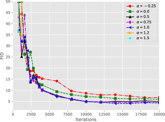
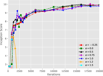
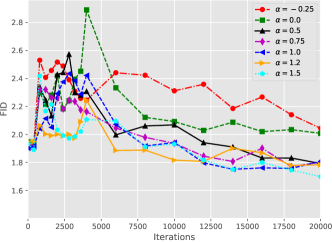
Figure 1: Ablation Study of $\alpha$ on distilling an EDM model pretrained on CIFAR-10 (unconditional): Each plot illustrates the relation between the performance, measured by FID (left) and Inception Score (right) vs. the number of training iterations during the distillation, across varying values of $\alpha$. The batch sizer is 256. The study underscores the impact of $\alpha$ on both training efficiency and generative fidelity, leading us to select $\alpha=1.0$ for the subsequent experiments.

Figure 2: Analogous plot for SiD²A, a SiD initialized SiDA model. We observe a trajectory of improvements in SiD²A over the SiD-distilled generator following an initial warmup period, and more robust performance in terms of the choice of $\alpha$.

5.1 Ablation on the choice of $\alpha$.

We conducted an ablation study to evaluate the impact of the gradient bias correction weight factor $\alpha$, a pivotal hyperparameter for SiD, on the performance of SiDA. Specifically, we tested a spectrum of $\alpha$ values $[-0.25,0.0,0.5,0.75,1.0,1.2,1.5]$ during the distillation of the EDM model pretrained on CIFAR-10 in an unconditional context. Figure 2 demonstrates how the model’s performance varies with different $\alpha$ values over the first 20k iterations at a batch size of 256, assessed using FID and IS. We determined that an $\alpha$ value of 1.0 yielded the best performance, prompting us to adopt this setting for subsequent experiments of SiDA over various datasets. In contrast, lower $\alpha$ values such as $-0.25$ or 0 resulted in suboptimal performance, while high values like 1.2 or 1.5 led to training instability and divergence. Interestingly, the performance disparity for $\alpha$ values between 0.5 and 1.0 was significantly narrower than those observed in SiD, as depicted in Figure 8 of Zhou et al. (2024b). These findings imply that although the adversarial loss may introduce some instability, it could also compensate for the inadequate correction of gradient biases associated with smaller $\alpha$ values.

In an alternative setting, referred to as SiD²A (SiD-initialized SiDA), where the generator $G_{\theta}$ is initialized using the best available pre-distilled SiD generator, we observe robust and stabilized training across all choices of $\alpha$. This suggests that initializing with the pre-distilled SiD generator provides a more advantageous starting point to achieve enhanced training stability and generative quality. Following these observations, and given that $\alpha=1.0$ and $\alpha=1.2$ were also utilized in SiD experiments, we have selected these same values for subsequent experiments with SiD²A.

Family Model NFE FID ($\downarrow$) IS ($\uparrow$) Teacher VP-EDM (Karras et al., 2022) 35 1.97 9.68 Diffusion DDPM (Ho et al., 2020) 1000 3.17 9.46 $\pm$ 0.11 DDIM (Song et al., 2020) 100 4.16 DPM-Solver-3 (Lu et al., 2022) 48 2.65 VDM (Kingma et al., 2021) 1000 4.00 iDDPM (Nichol & Dhariwal, 2021) 4000 2.90 HSIVI-SM (Yu et al., 2023) 15 4.17 TDPM+ (Zheng et al., 2022) 100 2.83 9.34 VP-EDM+LEGO-PR (Zheng et al., 2024) 35 1.88 9.84 One Step StyleGAN2+ADA+Tune (Karras et al., 2020) 1 2.92 $\pm$ 0.05 9.83 $\pm$ 0.04 Diffusion ProjectedGAN (Wang et al., 2023b) 1 2.54 iCT-deep (Song & Dhariwal, 2023) 1 2.51 9.76 Diff-Instruct (Luo et al., 2023b) 1 4.53 9.89 StyleGAN2+ADA+Tune+DI (Luo et al., 2023b) 1 2.71 9.86 $\pm$ 0.04 DMD (Yin et al., 2024b) 1 3.77 CTM (Kim et al., 2023) 1 1.98 GDD-I (Zheng & Yang, 2024) 1 1.54 10.10 SiD, $\alpha=1.0$ 1 2.028 $\pm$ 0.020 10.017 $\pm$ 0.047 SiD, $\alpha=1.2$ 1 1.923 $\pm$ 0.017 9.980 $\pm$ 0.042 SiDA, $\alpha=1.0$ 1 1.516 $\pm$ 0.010 10.323 $\pm$ 0.048 SiD²A, $\alpha=1.0$ 1 1.499 $\pm$ 0.012 10.188 $\pm$ 0.035 SiD²A, $\alpha=1.2$ 1 1.519 $\pm$ 0.009 10.252 $\pm$ 0.027

Table 1: Comparison of unconditional generation on CIFAR-10. The best one/few-step generator under the FID or IS metric is highlighted with bold.

Family Model FID ($\downarrow$) Teacher VP-EDM (Karras et al., 2022) 1.79 Direct generation BigGAN (Brock et al., 2019) 14.73 StyleGAN2+ADA (Karras et al., 2020) 3.49 $\pm$ 0.17 StyleGAN2+ADA+Tune (Karras et al., 2020) 2.42 $\pm$ 0.04 Distillation GET-Base (Geng et al., 2023) 6.25 Diff-Instruct (Luo et al., 2023b) 4.19 StyleGAN2+ADA+Tune+DI (Luo et al., 2023b) 2.27 DMD (Yin et al., 2024b) 2.66 DMD (w.o. KL) (Yin et al., 2024b) 3.82 DMD (w.o. reg.) (Yin et al., 2024b) 5.58 CTM (Kim et al., 2023) 1.73 GDD-I (Zheng & Yang, 2024) 1.44 SiD, $\alpha=1.0$ 1.932 $\pm$ 0.019 SiD , $\alpha=1.2$ 1.710 $\pm$ 0.011 SiDA, $\alpha=1.0$ 1.436 $\pm$ 0.009 SiD²A, $\alpha=1.0$ 1.403 $\pm$ 0.010 SiD²A, $\alpha=1.2$ 1.396 $\pm$ 0.014

Table 2: Analogous to Table 2 for CIFAR-10 (conditional). “Direct generation” and “Distillation” methods presented in the table requires one single NFE, and the teacher requires 35 NFE.

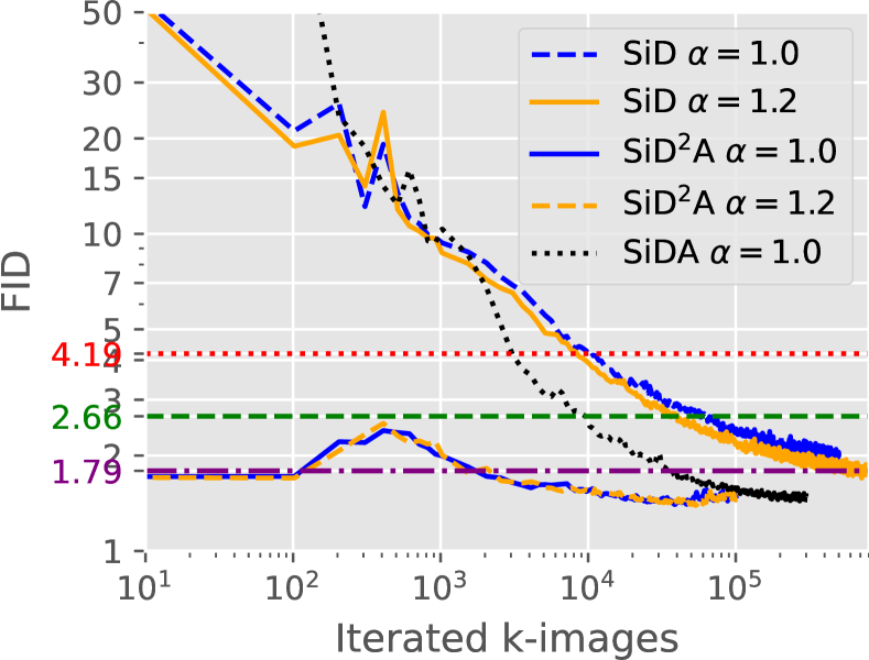
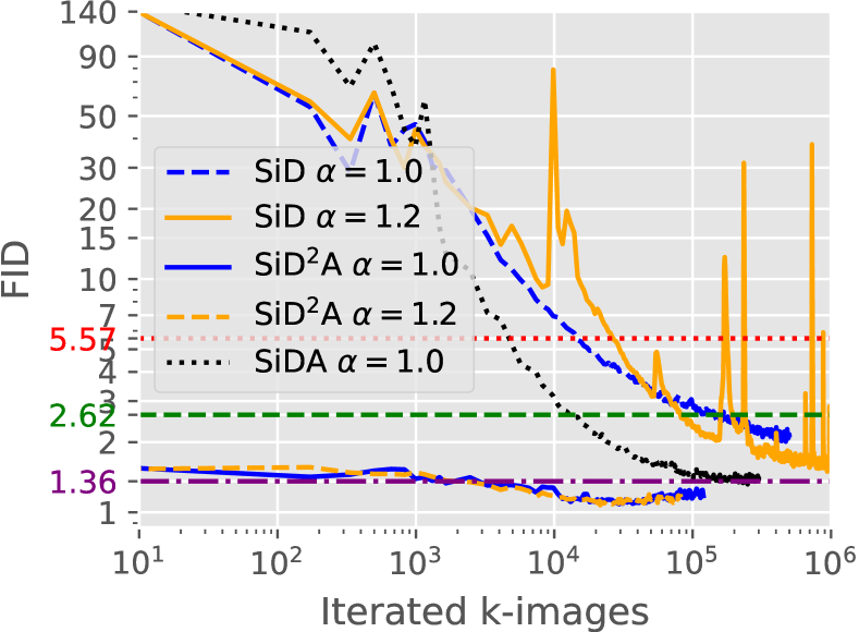
Figure 3: Evolution of FIDs for the SiD and SiDA generator during the distillation of the EDM teacher model pretrained on CIFAR-10 unconditional (left) and conditional (middle), with a batch size of 256, and on ImageNet 64x64 (right) with a batch size of 8192, using $\alpha=1.0$ or $\alpha=1.2$. The performance of EDM (35 NFEs), along with DMD and Diff-Instruct, is depicted with horizontal lines in purple, green, and red, respectively.

Table 3: Analogous to Table 2 for ImageNet 64x64 with label conditioning. The Precision and Recall metrics are also included.

Family Model NFE FID ($\downarrow$) Prec. ($\uparrow$) Rec. ($\uparrow$) Teacher VP-EDM (Karras et al., 2022) 511 1.36 79 2.64 0.71 0.67 Diffusion RIN (Jabri et al., 2022) 1000 1.23 DDPM (Ho et al., 2020) 250 11.00 0.67 0.58 ADM (Dhariwal & Nichol, 2021) 250 2.07 0.74 0.63 DPM-Solver-3 (Lu et al., 2022) 50 17.52 HSIVI-SM (Yu et al., 2023) 15 15.49 U-ViT (Bao et al., 2022) 50 4.26 DiT-L/2 (Peebles & Xie, 2023) 250 2.91 LEGO (Zheng et al., 2024) 250 2.16 Consistency iCT (Song & Dhariwal, 2023) 1 4.02 0.70 0.63 iCT-deep (Song & Dhariwal, 2023) 1 3.25 0.72 0.63 Distillation PD (Salimans & Ho, 2022) 2 8.95 0.63 0.65 G-distill (Meng et al., 2023) ($w$=0.3) 8 2.05 BOOT (Gu et al., 2023) 1 16.3 0.68 0.36 PID (Tee et al., 2024) 1 9.49 DFNO (Zheng et al., 2023) 1 7.83 0.61 CD-LPIPS (Song et al., 2023) 2 4.70 0.69 0.64 Diff-Instruct (Luo et al., 2023b) 1 5.57 TRACT (Berthelot et al., 2023) 2 4.97 DMD (Yin et al., 2024b) 1 2.62 CTM (Kim et al., 2023) 1 1.92 0.57 CTM (Kim et al., 2023) 2 1.73 0.57 GDD-I (Zheng & Yang, 2024) 1 1.16 0.75 0.60 EMD-16 (Xie et al., 2024) 1 2.2 0.59 DMD2  (Yin et al., 2024a) 1 1.51 DMD2+longer training  (Yin et al., 2024a) 1 1.28 SiD , $\alpha=1.0$ 1 2.022 $\pm$ 0.031 0.73 0.63 SiD , $\alpha=1.2$ 1 1.524 $\pm$ 0.009 0.74 0.63 SiDA, $\alpha=1.0$ (ours) 1 1.353 $\pm$ 0.025 0.74 0.63 SiD²A, $\alpha=1.0$ (ours) 1 1.114 $\pm$ 0.019 0.75 0.62 SiD²A, $\alpha=1.2$ (ours) 1 1.110 $\pm$ 0.018 0.75 0.62

5.2 Benchmarking EDM Distillation

We begin by assessing the performance of SiDA and SiD²A, focusing on both generation quality and convergence speed across the datasets previously mentioned. Our comprehensive evaluation compares SiDA and SiD²A against top-performing deep generative models, including GANs, traditional diffusion models, and their distilled counterparts, in terms of generation quality. Qualitatively, random images generated by SiD²A in a single step are displayed from Figures 6 to 10 in the Appendix, illustrating the high quality achieved.

Quantitatively, on CIFAR-10 in both conditional and unconditional settings, SiDA and SiD²A outperform leading models, with details in Tables 2 and 2. Notably, SiDA achieves an FID of 1.516, outperforming all baseline models. When leveraging the one-step generators already distilled by SiD for initialization, SiD²A further advances this performance, achieving an exceptionally low FID of 1.499 on CIFAR-10 unconditional with $\alpha=1.0$, and 1.396 on CIFAR-10 conditional with $\alpha=1.2$.

We further validate the effectiveness of SiDA and SiD²A on the ImageNet 64x64 dataset. Here, SiDA demonstrated superior performance over SiD, achieving an FID of 1.353. Notably, by leveraging the advanced capabilities of the SiD one-step generator, SiD²A attained an unprecedented low FID of 1.110 on ImageNet 64x64 with $\alpha=1.2$, surpassing the teacher model’s performance by a large margin. On the FFHQ 64x64 and AFHQ-v2 64x64 datasets, known for human and animal faces, SiDA and SiD²A again prove superior. The datasets’ less diverse patterns do not diminish the models’ performance, with SiDA and SiD²A maintaining faster convergence and surpassing the teacher model rapidly. The clear improvements across diverse datasets underscore SiDA and SiD²A’s effectiveness.

It’s worth noting that SiDA’s close competitor for ImageNet ($64\times 64$), GDD-I (Zheng & Yang, 2024), uses a discriminator inspired by Projected GAN (Sauer et al., 2021), integrating features from VGG16-BN and EfficientNet-lite0. Concerns have been raised, as discussed in Kynkäänniemi et al. (2023) and by Song & Dhariwal (2023), about the potential for encoders pretrained on ImageNet to inadvertently enhance FID scores through feature leakage. This potential issue does not affect SiD, SiDA, or SiD²A, ensuring our results reflect true model performance without such confounds.

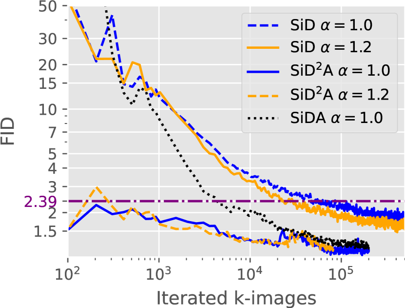
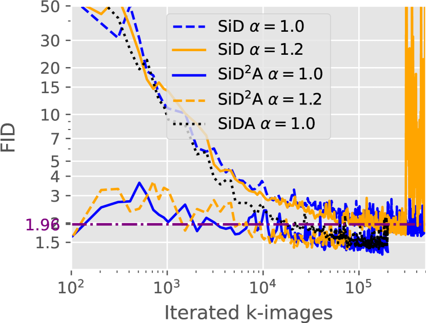
Figure 5: Analogous plot to Figure 3 for FFHQ-64x64 with batch size of 512 (left) and AFHQ-v2-64x64 with batch size of 512 (right).

SiDA also demonstrates accelerated convergence, as evidenced in Figures 3 and 5. The logarithmic scale plots show SiDA’s FID decreasing more rapidly than SiD’s, an efficiency that also holds when scaled up to ImageNet 64x64. Overall, SiDA consistently outperforms SiD in terms of convergence speed by a substantial margin, marking a significant acceleration, particularly noteworthy since SiD already converges at an exponential rate. This rapid improvement in both speed and performance underscores SiDA’s effectiveness and efficiency in generating high-quality images across different datasets. These results not only highlight SiD²A’s enhanced image quality and reduced iteration needs but also the overall efficiency of SiDA and SiD²A across various datasets, confirming the advantages of these advanced distillation techniques.

5.3 Benchmarking EDM2 Distillation

We validate the effectiveness of SiD, SiDA, and SiD²A in distilling EDM2 models of six different sizes pretrained on ImageNet 512x512. Our findings are summarized in Tables 4 and 7 and illustrated in Figure 4. Notably, SiD, our baseline single-step generator introduced six months ago on arXiv, performs comparably to the EDM2 teacher, which requires 63 NFEs, as well as to the simple, stable, and scalable consistency distillation (sCD) method of Lu & Song (2024) that uses 2 NFEs—a concurrent work to SiDA. SiD also convincingly outperforms sCD with 1 NFE, despite not yet employing CFG during distillation. Consistent with findings from EDM distillation, both SiDA and SiD²A demonstrate superior performance over SiD in distilling EDM2, achieving FIDs of 1.756 and 1.669, respectively, using the EDM2-S model with only 280M parameters. These results already surpass the EDM2-XXL model and sCD at 1.5B parameters, whose FIDs exceed 1.8.

Notably, scaling SiDA to EDM2-XL achieves a record-low FID of 1.449. While results for SiD²A on EDM2-XL and for the SiD family on EDM2-XXL are forthcoming, Figure 4 indicates the potential for further FID reductions as these results become available.

Mirroring findings from EDM distillation, SiDA also exhibits accelerated convergence when distilling EDM2, as shown in Figure 4. Logarithmic-scale plots reveal a more rapid decrease in FID for SiDA compared to SiD, an efficiency that scales effectively to ImageNet 512x512 and across generators of various sizes. Overall, SiDA consistently surpasses prior and concurrent methods in terms of both final metrics and convergence speed. This rapid improvement highlights SiDA’s effectiveness and efficiency in generating high-resolution images across various model sizes.

Table 4: FID scores and number of parameters for different methods on ImageNet (512x512).

Method	CFG	NFE	XS (125M)	S (280M)	M (498M)	L (777M)	XL (1.1B)	XXL (1.5B)
EDM2	N	63	3.53	2.56	2.25	2.06	1.96	1.91
EDM2	Y	63	2.91	2.23	2.01	1.88	1.85	1.81
sCT	Y	1	-	10.13	5.84	5.15	4.33	4.29
sCT	Y	2	-	9.86	5.53	4.65	3.73	3.76
sCD	Y	1	-	3.07	2.75	2.55	2.40	2.28
sCD	Y	2	-	2.50	2.26	2.04	1.93	1.88
SiD	N	1	3.353 $\pm$ 0.041	2.707 $\pm$ 0.054	2.060 $\pm$ 0.038	1.907 $\pm$ 0.016	2.005 $\pm$ 0.024	-
SiDA	N	1	2.228 $\pm$ 0.037	1.756 $\pm$ 0.023	1.546 $\pm$ 0.023	1.501 $\pm$ 0.024	1.449 $\pm$ 0.033	-
SiD2A	N	1	2.156 $\pm$ 0.028	1.669 $\pm$ 0.019	1.488 $\pm$ 0.038	1.465 $\pm$ 0.028	-	-

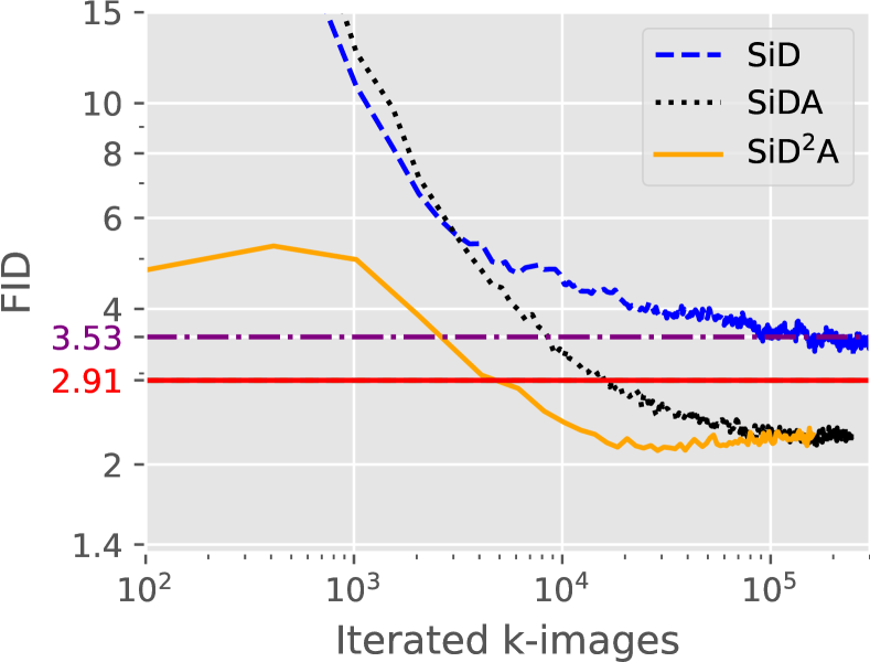
(a) EDM-XS

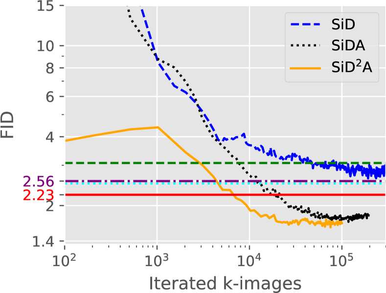
(b) EDM-S

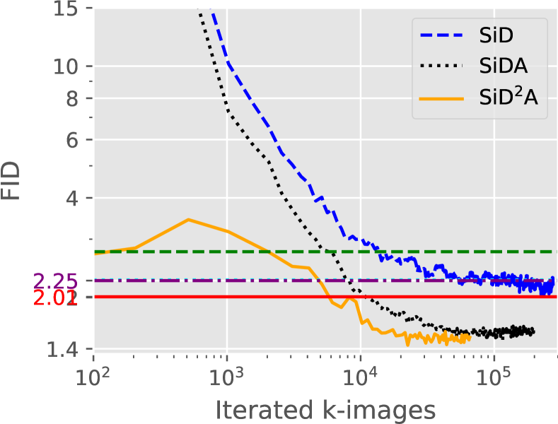
(c) EDM-M

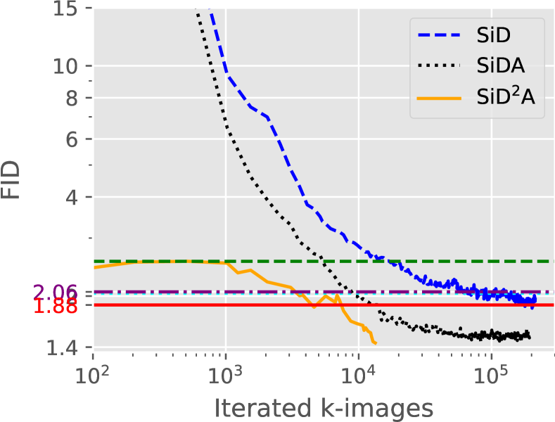
(d) EDM-L

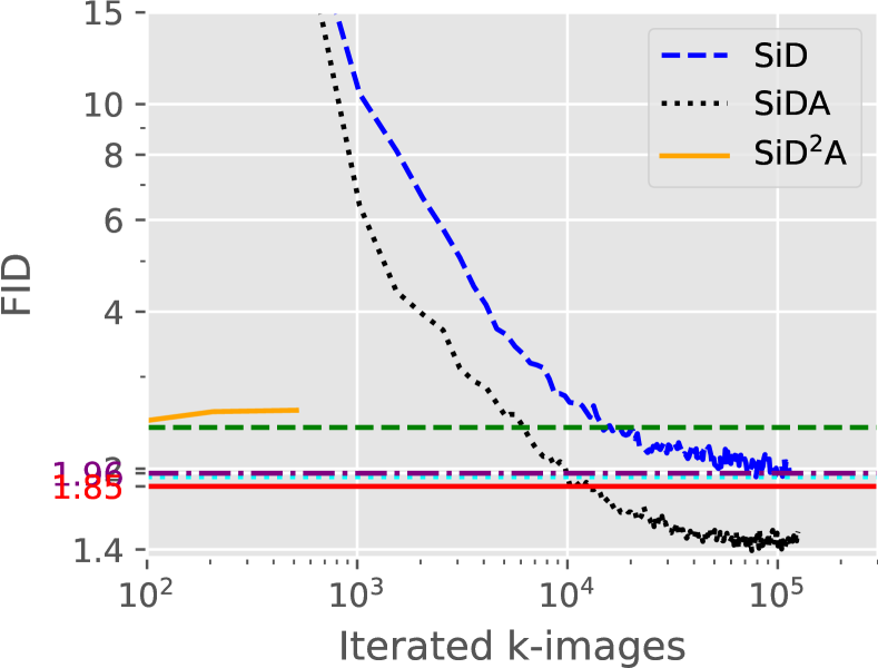
(e) EDM-XL

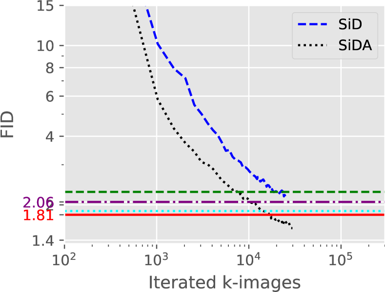
(f) EDM-XXL

Figure 4: Evolution of FIDs for the SiD and SiDA generators during the distillation of the EDM2 teacher models of six different sizes pretrained on ImageNet (512x512), with a batch size of 2048 and $\alpha=1.0$. The performance of EDM2 without classifier-free guidance (CFG) and EDM2 with CFG, using 64 NFEs, along with the simple, stable, and scalable consistency distillation (sCD) method of Lu & Song (2024) with 1 and 2 NFEs, is depicted with horizontal lines in purple, red, green, and cyan respectively.

6 Conclusion

In this paper, we present Score identity Distillation with Adversarial Loss (SiDA), an innovative framework that optimizes diffusion model distillation by integrating the strengths of Score identity Distillation (SiD) and Diffusion-GAN. SiDA accelerates the generation process, significantly reducing the number of iterations required compared to conventional score distillation methods, while producing high-quality images. Extensive tests across various datasets—CIFAR-10, ImageNet (64x64 and 512x512), FFHQ, AFHQ-v2—and different scales of pretrained EDM2 models demonstrate that SiDA consistently surpasses both the base teacher diffusion models and other distilled variants. This is validated by superior Fréchet Inception Distance (FID) scores and other performance metrics. Notably, SiDA achieves these results without utilizing classifier-free guidance, suggesting potential for further enhancement with its integration. Specifically, incorporating the long-and-short guidance strategy as described by Zhou et al. (2024a) could further refine SiDA’s performance. Future work will explore expanding SiDA’s methodology to additional generative tasks and refining its capabilities through innovative distillation techniques.

Appendix for SiDA

Appendix A Algorithm Box

Algorithm 1 Adversarial Score identity Distillation (SiDA)

1:  Input: Pretrained score network $f_{\phi}$, generator $G_{\theta}$, generator score network $f_{\psi}$, $\sigma_{\text{init}}=2.5$, $t_{\max}=800$, $\alpha=1.2$, $\lambda_{\text{sid}}=100$, $\lambda_{\text{adv}}=0.01$, image size $(W,H,C_{c})$, latent discriminator map size $(W^{\prime},H^{\prime})$.

2:  Initialization $\theta\leftarrow\phi,\psi\leftarrow\phi$, $D(\cdot)\leftarrow\text{encoder}(\psi)$

3:  repeat

4:     Sample $\boldsymbol{z}\sim\mathcal{N}(0,\mathbf{I})$ and $\boldsymbol{x}_{g}=G_{\theta}(\sigma_{\text{init}}\boldsymbol{z})$

5:     Sample $t\sim p(t),~{}\boldsymbol{\epsilon}_{t}\sim\mathcal{N}(0,\mathbf{I})$ and $\boldsymbol{x}_{t}=a_{t}\boldsymbol{x}_{g}+\sigma_{t}\boldsymbol{\epsilon}_{t}$

6:     Update $\psi$ with 9:

7:         $\mathcal{L}_{\psi}^{(\text{sida})}={\gamma(t)}(\|f_{\psi}(\boldsymbol{x}_{t},t)-\boldsymbol{x}_{g}\|_{2}^{2}+{L}_{\psi}^{(\text{adv})})$

8:         $\psi=\psi-\eta\nabla_{\psi}\mathcal{L}_{\psi}^{(\text{sida})}$

9:     where the timestep distribution $t\sim p(t)$, noise level $\sigma_{t}$, and weighting function $\gamma(t)$ are defined as in Zhou et al. (2024b).

10:     if num_imgs $\geq$ 100K then

11:        Sample $t\sim\mbox{Unif}[0,t_{\max}/1000]$, compute $\sigma_{t}$, $\omega_{t}$ and $a_{t}$ as defined in Zhou et al. (2024b)

12:        Set $b=0$ if num_imgs $\leq$200k and $b=1$ otherwise

13:        Update $G_{\theta}$ with 8:

14:            $\mathcal{L}_{\theta}^{(\text{sida})}=\displaystyle\big{(}\frac{1}{2}\big{)}^{b}\lambda_{\text{sid}}\left((1-\alpha)\frac{\omega(t)a_{t}^{2}}{{\sigma_{t}^{4}}}\|f_{\phi}(\boldsymbol{x}_{t},t)-f_{\psi}(\boldsymbol{x}_{t},t)\|_{2}^{2}\right.$

15:                  $\displaystyle\left.+\frac{\omega(t)a_{t}^{2}}{{\sigma_{t}^{4}}}(f_{\phi}(\boldsymbol{x}_{t},t)-f_{\psi}(\boldsymbol{x}_{t},t))^{T}(f_{\psi}(\boldsymbol{x}_{t},t)-\boldsymbol{x}_{g})\right)+\frac{b}{2}\lambda_{\text{adv}}\frac{\omega(t)a_{t}^{2}}{2\sigma_{t}^{4}}{C_{c}WH}\mathcal{L}_{\theta}^{(\text{adv})}$

16:            $\theta=\theta-\eta\nabla_{\theta}\mathcal{L}_{\theta}^{(\text{sida})}$

17:     end if

18:  until the FID plateaus or the training budget is exhausted

19:  Output: $G_{\theta}$

Algorithm 2 SiD²A: SiD initilized SiDA

1:  Extra Input: Pretrained SiD generator $\theta_{\text{sid}}$

2:  Initialization $\theta\leftarrow\theta_{\text{sid}},\psi\leftarrow\phi$ , $D(\cdot)\leftarrow\text{encoder}(\psi)$

3:  repeat

4:     The same as SiDA

5:  until the FID plateaus or the training budget is exhausted

6:  Output: $G_{\theta}$

Appendix B Additional Training and Evaluation Details

Table 5: Analogous to Table 2 for FFHQ 64x64.

Family Model NFE FID ($\downarrow$) Teacher VP-EDM (Karras et al., 2022) 79 2.39 Diffusion VP-EDM (Karras et al., 2022) 50 2.60 Patch-Diffusion (Wang et al., 2023a) 50 3.11 Distillation BOOT (Gu et al., 2023) 1 9.00 SiD, $\alpha=1.0$ 1 1.710 $\pm$ 0.018 SiD, $\alpha=1.2$ 1 1.550 $\pm$ 0.017 SiDA, $\alpha=1.0$ (ours) 1 1.134$\pm$ 0.012 SiD²A, $\alpha=1.0$ (ours) 1 1.040 $\pm$ 0.011 SiD²A, $\alpha=1.2$ (ours) 1 1.109 $\pm$ 0.015

Table 6: Analogous to Table 2 for AFHQ-v2 64x64.

Family Model NFE FID ($\downarrow$) Teacher VP-EDM (Karras et al., 2022) 79 1.96 Distillation SiD, $\alpha=1.0$ 1 1.628 $\pm$ 0.017 SiD, $\alpha=1.2$ 1 1.711 $\pm$ 0.020 SiDA, $\alpha=1.0$ (ours) 1 1.345 $\pm$ 0.015 SiD²A, $\alpha=1.0$ (ours) 1 1.276 $\pm$ 0.010 SiD²A, $\alpha=1.2$ (ours) 1 1.366 $\pm$ 0.018

Table 7: FD${}_{\text{DINOv2}}$ scores and number of parameters for different methods on ImageNet (512x512).

Method	CFG	NFE	XS (125M)	S (280M)	M (498M)	L (777M)	XL (1.1B)	XXL (1.5B)
EDM2	N	63	103.39	68.64	58.44	52.25	45.96	42.84
EDM2	Y	63	79.94	52.32	41.98	38.20	35.67	33.09
SiD	N	1	91.75 $\pm$ 0.55	65.08 $\pm$ 0.32	55.92 $\pm$ 0.25	56.25 $\pm$ 0.40	55.87 $\pm$ 0.21	-
SiDA	N	1	93.67 $\pm$ 0.40	68.76 $\pm$ 0.45	53.40 $\pm$ 0.60	48.47 $\pm$ 0.45	46.47 $\pm$ 0.27	-
SiD2A	N	1	86.96 $\pm$ 0.32	62.19 $\pm$ 0.36	49.01 $\pm$ 0.54	45.92 $\pm$ 0.33	-	-

The hyperparameters customized for our study are outlined in Table 8, with all remaining settings consistent with those in the EDM code (Karras et al., 2022) and SiD code (Zhou et al., 2024b).

Table 8: Hyperparameter settings and comparison of distillation time, and memory usage between SiD and SiDA, using 8 NVIDIA V100 GPUs (16 GB each) or 8 NVIDIA H100 GPUs (80 GB each).

Method	Hyperparameters	CIFAR-10 32x32	ImageNet 64x64	FFHQ 64x64	AFHQ-v2 64x64
	Batch size	256	8192	512	512
	Batch size per GPU	32	32	64	64
	GPUs	8xV100	8xH100	8xH100	8xH100
	Gradient accumulation round	1	32	1	1
	Learning rate of ($\psi$, $\theta$)	1e-5	4e-6	1e-5	5e-6
	Loss scaling of ($\lambda_{\text{sid}},\,\lambda_{\text{adv}}$)	(100, 0.01)
	ema	0.5	2	0.5	0.5
	fp16	False	True	True	True
	Optimizer Adam (eps)	1e-8	1e-6	1e-6	1e-6
	Optimizer Adam ($\beta_{1}$)	0
	Optimizer Adam ($\beta_{2}$)	0.999
	$\alpha$	$1.0$ for SiDA; both $1.0$ and $1.2$ for SiD2A
	$\sigma_{\text{init}}$	2.5
	$t_{\max}$	800
	augment, dropout, cres	The same as in EDM and SiD for each corresponding dataset
SiD	max memory allocated per GPU	13.0	46.7	31.1	31.1
	max memory in GB reserved per GPU	13.3	48.0	31.3	31.3
	$\sim$seconds per 1k images	3.3	3.1	1.1	1.1
	$\sim$hours per 10M ($10^{4}$k) images	9.2	8.6	3.1	3.1
	$\sim$days per 100M ($10^{5}$k) images	3.8	3.6	1.3	1.3
SiDA	max memory allocated per GPU	13.0	46.7	31.1	31.1
	max memory in GB reserved per GPU	13.4	48.1	31.3	31.3
	$\sim$seconds per 1k images	3.6	3.5	1.2	1.2
	$\sim$hours per 10M ($10^{4}$k) images	10.0	9.7	3.3	3.3
	$\sim$days per 100M ($10^{5}$k) images	4.2	4.1	1.4	1.4

Figure 6: Unconditional CIFAR-10 32X32 random images generated with SiD²A (FID: 1.499).

Figure 7: Label conditioning CIFAR-10 32X32 random images generated with SiD²A (FID: 1.396)

Figure 8: Label conditioning ImageNet 64x64 random images generated with SiD²A (FID: 1.110)

Figure 9: FFHQ 64X64 random images generated with SiD²A (FID: 1.040)

Figure 10: AFHQ-V2 64X64 random images generated with SiD²A (FID: 1.276)

References

- Arjovsky et al. (2017) Martin Arjovsky, Soumith Chintala, and Léon Bottou. Wasserstein generative adversarial networks. In Proceedings of the 34th International Conference on Machine Learning-Volume 70, pp. 214–223, 2017.
- Bao et al. (2022) Fan Bao, Chongxuan Li, Yue Cao, and Jun Zhu. All are worth words: A ViT backbone for score-based diffusion models. arXiv preprint arXiv:2209.12152, 2022.
- Berthelot et al. (2023) David Berthelot, Arnaud Autef, Jierui Lin, Dian Ang Yap, Shuangfei Zhai, Siyuan Hu, Daniel Zheng, Walter Talbott, and Eric Gu. Tract: Denoising diffusion models with transitive closure time-distillation. arXiv preprint arXiv:2303.04248, 2023.
- Bishop (2006) Christopher M Bishop. Pattern Recognition and Machine Learning. springer, 2006.
- Blei & Jordan (2006) D. M. Blei and M. I. Jordan. Variational inference for Dirichlet process mixtures. Bayesian analysis, 1(1):121–143, 2006.
- Blei et al. (2003) David M Blei, Andrew Y Ng, and Michael I Jordan. Latent dirichlet allocation. Journal of Machine Learning Research, 3:993–1022, 2003.
- Brock et al. (2019) Andrew Brock, Jeff Donahue, and Karen Simonyan. Large scale GAN training for high fidelity natural image synthesis. In International Conference on Learning Representations, 2019. URL https://openreview.net/forum?id=B1xsqj09Fm.
- Choi et al. (2020) Yunjey Choi, Youngjung Uh, Jaejun Yoo, and Jung-Woo Ha. Stargan v2: Diverse image synthesis for multiple domains. In Proceedings of the IEEE/CVF conference on computer vision and pattern recognition, pp. 8188–8197, 2020.
- Chong et al. (2009) Wang Chong, David Blei, and Fei-Fei Li. Simultaneous image classification and annotation. In 2009 IEEE Conference on computer vision and pattern recognition, pp. 1903–1910. IEEE, 2009.
- Deng et al. (2009) Jia Deng, Wei Dong, Richard Socher, Li-Jia Li, Kai Li, and Li Fei-Fei. ImageNet: A large-scale hierarchical image database. In 2009 IEEE conference on computer vision and pattern recognition, pp. 248–255. Ieee, 2009.
- Dhariwal & Nichol (2021) Prafulla Dhariwal and Alexander Nichol. Diffusion models beat GANs on image synthesis. Advances in Neural Information Processing Systems, 34:8780–8794, 2021.
- Fei-Fei & Perona (2005) Li Fei-Fei and Pietro Perona. A Bayesian hierarchical model for learning natural scene categories. In 2005 IEEE computer society conference on computer vision and pattern recognition (CVPR’05), volume 2, pp. 524–531. IEEE, 2005.
- Geng et al. (2023) Zhengyang Geng, Ashwini Pokle, and J Zico Kolter. One-step diffusion distillation via deep equilibrium models. Advances in Neural Information Processing Systems, 36, 2023.
- Goodfellow et al. (2014) Ian Goodfellow, Jean Pouget-Abadie, Mehdi Mirza, Bing Xu, David Warde-Farley, Sherjil Ozair, Aaron Courville, and Yoshua Bengio. Generative adversarial nets. In Advances in Neural Information Processing Systems, pp. 2672–2680, 2014.
- Goodfellow et al. (2016) Ian Goodfellow, Yoshua Bengio, and Aaron Courville. Deep Learning. MIT Press, 2016. http://www.deeplearningbook.org.
- Griffiths & Ghahramani (2005) T. L. Griffiths and Z. Ghahramani. Infinite latent feature models and the Indian buffet process. In NIPS, 2005.
- Gu et al. (2023) Jiatao Gu, Shuangfei Zhai, Yizhe Zhang, Lingjie Liu, and Joshua M Susskind. BOOT: Data-free distillation of denoising diffusion models with bootstrapping. In ICML 2023 Workshop on Structured Probabilistic Inference and Generative Modeling, 2023.
- Hang et al. (2023) Tiankai Hang, Shuyang Gu, Chen Li, Jianmin Bao, Dong Chen, Han Hu, Xin Geng, and Baining Guo. Efficient diffusion training via min-snr weighting strategy. arXiv preprint arXiv:2303.09556, 2023.
- Hinton et al. (2006) G. Hinton, S. Osindero, and Y.-W. Teh. A fast learning algorithm for deep belief nets. Neural Computation, 18(7):1527–1554, 2006.
- Hinton (2002) Geoffrey E Hinton. Training products of experts by minimizing contrastive divergence. Neural computation, 14(8):1771–1800, 2002.
- Ho et al. (2020) Jonathan Ho, Ajay Jain, and Pieter Abbeel. Denoising Diffusion Probabilistic Models. Advances in Neural Information Processing Systems, 33, 2020.
- Hoffman et al. (2013) Matthew D Hoffman, David M Blei, Chong Wang, and John Paisley. Stochastic variational inference. The Journal of Machine Learning Research, 14(1):1303–1347, 2013.
- Jabri et al. (2022) Allan Jabri, David Fleet, and Ting Chen. Scalable adaptive computation for iterative generation. arXiv preprint arXiv:2212.11972, 2022.
- Karras et al. (2019) Tero Karras, Samuli Laine, and Timo Aila. A style-based generator architecture for generative adversarial networks. In Proceedings of the IEEE/CVF conference on computer vision and pattern recognition, pp. 4401–4410, 2019.
- Karras et al. (2020) Tero Karras, Samuli Laine, Miika Aittala, Janne Hellsten, Jaakko Lehtinen, and Timo Aila. Analyzing and improving the image quality of StyleGAN. In Proc. CVPR, 2020.
- Karras et al. (2022) Tero Karras, Miika Aittala, Timo Aila, and Samuli Laine. Elucidating the design space of diffusion-based generative models. In Alice H. Oh, Alekh Agarwal, Danielle Belgrave, and Kyunghyun Cho (eds.), Advances in Neural Information Processing Systems, 2022. URL https://openreview.net/forum?id=k7FuTOWMOc7.
- Karras et al. (2024) Tero Karras, Miika Aittala, Jaakko Lehtinen, Janne Hellsten, Timo Aila, and Samuli Laine. Analyzing and improving the training dynamics of diffusion models. In Proceedings of the IEEE/CVF Conference on Computer Vision and Pattern Recognition, pp. 24174–24184, 2024.
- Kim et al. (2023) Dongjun Kim, Chieh-Hsin Lai, Wei-Hsiang Liao, Naoki Murata, Yuhta Takida, Toshimitsu Uesaka, Yutong He, Yuki Mitsufuji, and Stefano Ermon. Consistency trajectory models: Learning probability flow ode trajectory of diffusion. arXiv preprint arXiv:2310.02279, 2023.
- Kingma & Welling (2014) Diederik P. Kingma and Max Welling. Auto-encoding variational Bayes. In International Conference on Learning Representations, 2014.
- Kingma et al. (2021) Diederik P Kingma, Tim Salimans, Ben Poole, and Jonathan Ho. Variational diffusion models. arXiv preprint arXiv:2107.00630, 2021.
- Krizhevsky et al. (2009) Alex Krizhevsky et al. Learning multiple layers of features from tiny images. 2009.
- Kynkäänniemi et al. (2019) Tuomas Kynkäänniemi, Tero Karras, Samuli Laine, Jaakko Lehtinen, and Timo Aila. Improved precision and recall metric for assessing generative models. Advances in neural information processing systems, 32, 2019.
- Kynkäänniemi et al. (2023) Tuomas Kynkäänniemi, Tero Karras, Miika Aittala, Timo Aila, and Jaakko Lehtinen. The role of imagenet classes in fréchet inception distance. In The Eleventh International Conference on Learning Representations, 2023. URL https://openreview.net/forum?id=4oXTQ6m_ws8.
- Li et al. (2017) Chun-Liang Li, Wei-Cheng Chang, Yu Cheng, Yiming Yang, and Barnabás Póczos. MMD GAN: Towards deeper understanding of moment matching network. In Advances in Neural Information Processing Systems, pp. 2203–2213, 2017.
- Liu et al. (2023) Xingchao Liu, Xiwen Zhang, Jianzhu Ma, Jian Peng, and Qiang Liu. Instaflow: One step is enough for high-quality diffusion-based text-to-image generation. arXiv preprint arXiv:2309.06380, 2023.
- Lu & Song (2024) Cheng Lu and Yang Song. Simplifying, stabilizing and scaling continuous-time consistency models. arXiv preprint arXiv:2410.11081, 2024.
- Lu et al. (2022) Cheng Lu, Yuhao Zhou, Fan Bao, Jianfei Chen, Chongxuan Li, and Jun Zhu. DPM-solver: A fast ODE solver for diffusion probabilistic model sampling in around 10 steps. In Alice H. Oh, Alekh Agarwal, Danielle Belgrave, and Kyunghyun Cho (eds.), Advances in Neural Information Processing Systems, 2022. URL https://openreview.net/forum?id=2uAaGwlP_V.
- Luhman & Luhman (2021) Eric Luhman and Troy Luhman. Knowledge distillation in iterative generative models for improved sampling speed. arXiv preprint arXiv:2101.02388, 2021.
- Luo et al. (2023a) Simian Luo, Yiqin Tan, Longbo Huang, Jian Li, and Hang Zhao. Latent consistency models: Synthesizing high-resolution images with few-step inference. ArXiv, abs/2310.04378, 2023a.
- Luo et al. (2023b) Weijian Luo, Tianyang Hu, Shifeng Zhang, Jiacheng Sun, Zhenguo Li, and Zhihua Zhang. Diff-Instruct: A universal approach for transferring knowledge from pre-trained diffusion models. In Thirty-seventh Conference on Neural Information Processing Systems, 2023b. URL https://openreview.net/forum?id=MLIs5iRq4w.
- Luo et al. (2024) Weijian Luo, Zemin Huang, Zhengyang Geng, J Zico Kolter, and Guo-jun Qi. One-step diffusion distillation through score implicit matching. arXiv preprint arXiv:2410.16794, 2024.
- Lyu et al. (2022) Zhaoyang Lyu, Xudong Xu, Ceyuan Yang, Dahua Lin, and Bo Dai. Accelerating diffusion models via early stop of the diffusion process. arXiv preprint arXiv:2205.12524, 2022.
- Meng et al. (2023) Chenlin Meng, Robin Rombach, Ruiqi Gao, Diederik Kingma, Stefano Ermon, Jonathan Ho, and Tim Salimans. On distillation of guided diffusion models. In Proceedings of the IEEE/CVF Conference on Computer Vision and Pattern Recognition, pp. 14297–14306, 2023.
- Murphy (2012) Kevin P Murphy. Machine Learning: A Probabilistic Perspective. MIT Press, 2012.
- Nguyen & Tran (2024) Thuan Hoang Nguyen and Anh Tran. SwiftBrush: One-step text-to-image diffusion model with variational score distillation. In IEEE/CVF Conference on Computer Vision and Pattern Recognition (CVPR), 2024.
- Nichol & Dhariwal (2021) Alexander Quinn Nichol and Prafulla Dhariwal. Improved denoising diffusion probabilistic models. In International Conference on Machine Learning, pp. 8162–8171. PMLR, 2021.
- Nichol et al. (2022) Alexander Quinn Nichol, Prafulla Dhariwal, Aditya Ramesh, Pranav Shyam, Pamela Mishkin, Bob Mcgrew, Ilya Sutskever, and Mark Chen. Glide: Towards photorealistic image generation and editing with text-guided diffusion models. In International Conference on Machine Learning, pp. 16784–16804. PMLR, 2022.
- Oquab et al. (2023) Maxime Oquab, Timothée Darcet, Théo Moutakanni, Huy Vo, Marc Szafraniec, Vasil Khalidov, Pierre Fernandez, Daniel Haziza, Francisco Massa, Alaaeldin El-Nouby, et al. DINOv2: Learning robust visual features without supervision. arXiv preprint arXiv:2304.07193, 2023.
- Papamakarios et al. (2019) George Papamakarios, Eric Nalisnick, Danilo Jimenez Rezende, Shakir Mohamed, and Balaji Lakshminarayanan. Normalizing flows for probabilistic modeling and inference. arXiv preprint arXiv:1912.02762, 2019.
- Peebles & Xie (2023) William Peebles and Saining Xie. Scalable diffusion models with transformers. In Proceedings of the IEEE/CVF International Conference on Computer Vision, pp. 4195–4205, 2023.
- Podell et al. (2024) Dustin Podell, Zion English, Kyle Lacey, Andreas Blattmann, Tim Dockhorn, Jonas Müller, Joe Penna, and Robin Rombach. SDXL: Improving latent diffusion models for high-resolution image synthesis. In The Twelfth International Conference on Learning Representations, 2024. URL https://openreview.net/forum?id=di52zR8xgf.
- Poole et al. (2023) Ben Poole, Ajay Jain, Jonathan T. Barron, and Ben Mildenhall. DreamFusion: Text-to-3D using 2D diffusion. In The Eleventh International Conference on Learning Representations, 2023. URL https://openreview.net/forum?id=FjNys5c7VyY.
- Ramesh et al. (2022) Aditya Ramesh, Prafulla Dhariwal, Alex Nichol, Casey Chu, and Mark Chen. Hierarchical text-conditional image generation with CLIP latents. arXiv preprint arXiv:2204.06125, 2022.
- Reed et al. (2016) Scott Reed, Zeynep Akata, Xinchen Yan, Lajanugen Logeswaran, Bernt Schiele, and Honglak Lee. Generative adversarial text to image synthesis. In International conference on machine learning, pp. 1060–1069. PMLR, 2016.
- Rezende et al. (2014) Danilo Jimenez Rezende, Shakir Mohamed, and Daan Wierstra. Stochastic backpropagation and approximate inference in deep generative models. In Proceedings of the 31st International Conference on Machine Learning, pp. 1278–1286, 2014.
- Rombach et al. (2022) Robin Rombach, Andreas Blattmann, Dominik Lorenz, Patrick Esser, and Björn Ommer. High-resolution image synthesis with latent diffusion models. In Proceedings of the IEEE/CVF conference on computer vision and pattern recognition, pp. 10684–10695, 2022.
- Saharia et al. (2022) Chitwan Saharia, William Chan, Saurabh Saxena, Lala Li, Jay Whang, Emily L Denton, Kamyar Ghasemipour, Raphael Gontijo Lopes, Burcu Karagol Ayan, Tim Salimans, Jonathan Ho, David J Fleet, and Mohammad Norouzi. Photorealistic text-to-image diffusion models with deep language understanding. Advances in Neural Information Processing Systems, 35:36479–36494, 2022.
- Salakhutdinov & Hinton (2009) Ruslan Salakhutdinov and Geoffrey Hinton. Deep Boltzmann machines. In Artificial intelligence and statistics, pp. 448–455. PMLR, 2009.
- Salimans & Ho (2022) Tim Salimans and Jonathan Ho. Progressive distillation for fast sampling of diffusion models. In International Conference on Learning Representations, 2022. URL https://openreview.net/forum?id=TIdIXIpzhoI.
- Salimans et al. (2016) Tim Salimans, Ian Goodfellow, Wojciech Zaremba, Vicki Cheung, Alec Radford, and Xi Chen. Improved techniques for training GANs. In Advances in Neural Information Processing Systems, pp. 2234–2242, 2016.
- Sauer et al. (2021) Axel Sauer, Kashyap Chitta, Jens Müller, and Andreas Geiger. Projected gans converge faster. Advances in Neural Information Processing Systems, 34:17480–17492, 2021.
- Sauer et al. (2023) Axel Sauer, Dominik Lorenz, A. Blattmann, and Robin Rombach. Adversarial diffusion distillation. ArXiv, abs/2311.17042, 2023.
- Sohl-Dickstein et al. (2015) Jascha Sohl-Dickstein, Eric Weiss, Niru Maheswaranathan, and Surya Ganguli. Deep unsupervised learning using nonequilibrium thermodynamics. In International Conference on Machine Learning, pp. 2256–2265. PMLR, 2015.
- Song et al. (2020) Jiaming Song, Chenlin Meng, and Stefano Ermon. Denoising diffusion implicit models. In International Conference on Learning Representations, 2020.
- Song & Dhariwal (2023) Yang Song and Prafulla Dhariwal. Improved techniques for training consistency models. arXiv preprint arXiv:2310.14189, 2023.
- Song & Ermon (2019) Yang Song and Stefano Ermon. Generative Modeling by Estimating Gradients of the Data Distribution. In Advances in Neural Information Processing Systems, pp. 11918–11930, 2019.
- Song et al. (2023) Yang Song, Prafulla Dhariwal, Mark Chen, and Ilya Sutskever. Consistency models. arXiv preprint arXiv:2303.01469, 2023.
- Tee et al. (2024) Joshua Tian Jin Tee, Kang Zhang, Chanwoo Kim, Dhananjaya Nagaraja Gowda, Hee Suk Yoon, and Chang D. Yoo. Physics informed distillation for diffusion models, 2024. URL https://openreview.net/forum?id=a24gfxA7jD.
- Vincent (2011) Pascal Vincent. A Connection Between Score Matching and Denoising Autoencoders. Neural Computation, 23(7):1661–1674, 2011.
- Vincent et al. (2010) Pascal Vincent, Hugo Larochelle, Isabelle Lajoie, Yoshua Bengio, Pierre-Antoine Manzagol, and Léon Bottou. Stacked denoising autoencoders: Learning useful representations in a deep network with a local denoising criterion. Journal of machine learning research, 11(12), 2010.
- Wang et al. (2023a) Zhendong Wang, Yifan Jiang, Huangjie Zheng, Peihao Wang, Pengcheng He, Zhangyang Wang, Weizhu Chen, and Mingyuan Zhou. Patch diffusion: Faster and more data-efficient training of diffusion models. arXiv preprint arXiv:2304.12526, 2023a.
- Wang et al. (2023b) Zhendong Wang, Huangjie Zheng, Pengcheng He, Weizhu Chen, and Mingyuan Zhou. Diffusion-GAN: Training GANs with diffusion. In The Eleventh International Conference on Learning Representations, 2023b. URL https://openreview.net/forum?id=HZf7UbpWHuA.
- Wang et al. (2023c) Zhengyi Wang, Cheng Lu, Yikai Wang, Fan Bao, Chongxuan Li, Hang Su, and Jun Zhu. ProlificDreamer: High-fidelity and diverse text-to-3D generation with variational score distillation, 2023c.
- Xiao et al. (2022) Zhisheng Xiao, Karsten Kreis, and Arash Vahdat. Tackling the generative learning trilemma with denoising diffusion GANs. In International Conference on Learning Representations, 2022. URL https://openreview.net/forum?id=JprM0p-q0Co.
- Xie et al. (2024) Sirui Xie, Zhisheng Xiao, Diederik P Kingma, Tingbo Hou, Ying Nian Wu, Kevin Patrick Murphy, Tim Salimans, Ben Poole, and Ruiqi Gao. EM distillation for one-step diffusion models, 2024. URL https://arxiv.org/abs/2405.16852.
- Xu et al. (2023) Yanwu Xu, Yang Zhao, Zhisheng Xiao, and Tingbo Hou. UFOGen: You forward once large scale text-to-image generation via diffusion GANs. ArXiv, abs/2311.09257, 2023.
- Yin & Zhou (2018) Mingzhang Yin and Mingyuan Zhou. Semi-implicit variational inference. In International Conference on Machine Learning, pp. 5660–5669, 2018.
- Yin et al. (2024a) Tianwei Yin, Michaël Gharbi, Taesung Park, Richard Zhang, Eli Shechtman, Fredo Durand, and William T Freeman. Improved distribution matching distillation for fast image synthesis. arXiv preprint arXiv:2405.14867, 2024a.
- Yin et al. (2024b) Tianwei Yin, Michaël Gharbi, Richard Zhang, Eli Shechtman, Fredo Durand, William T Freeman, and Taesung Park. One-step diffusion with distribution matching distillation. In Proceedings of the IEEE/CVF Conference on Computer Vision and Pattern Recognition, pp. 6613–6623, 2024b.
- Yu et al. (2023) Longlin Yu, Tianyu Xie, Yu Zhu, Tong Yang, Xiangyu Zhang, and Cheng Zhang. Hierarchical semi-implicit variational inference with application to diffusion model acceleration. In Thirty-seventh Conference on Neural Information Processing Systems, 2023. URL https://openreview.net/forum?id=ghIBaprxsV.
- Zheng & Yang (2024) Bowen Zheng and Tianming Yang. Diffusion models are innate one-step generators. arXiv preprint arXiv:2405.20750, 2024.
- Zheng et al. (2023) Hongkai Zheng, Weili Nie, Arash Vahdat, Kamyar Azizzadenesheli, and Anima Anandkumar. Fast sampling of diffusion models via operator learning. In International Conference on Machine Learning, pp. 42390–42402. PMLR, 2023.
- Zheng & Zhou (2021) Huangjie Zheng and Mingyuan Zhou. Exploiting chain rule and Bayes’ theorem to compare probability distributions. Advances in Neural Information Processing Systems, 34:14993–15006, 2021.
- Zheng et al. (2022) Huangjie Zheng, Pengcheng He, Weizhu Chen, and Mingyuan Zhou. Truncated diffusion probabilistic models. arXiv preprint arXiv:2202.09671, 2022.
- Zheng et al. (2024) Huangjie Zheng, Zhendong Wang, Jianbo Yuan, Guanghan Ning, Pengcheng He, Quanzeng You, Hongxia Yang, and Mingyuan Zhou. Learning stackable and skippable LEGO bricks for efficient, reconfigurable, and variable-resolution diffusion modeling. In The Twelfth International Conference on Learning Representations, 2024. URL https://openreview.net/forum?id=qmXedvwrT1.
- Zhou et al. (2009) Mingyuan Zhou, Haojun Chen, John Paisley, Lu Ren, Guillermo Sapiro, and Lawrence Carin. Non-parametric Bayesian dictionary learning for sparse image representations. Advances in neural information processing systems, 22, 2009.
- Zhou et al. (2024a) Mingyuan Zhou, Zhendong Wang, Huangjie Zheng, and Hai Huang. Long and short guidance in score identity distillation for one-step text-to-image generation. arXiv preprint arXiv:2406.01561, 2024a.
- Zhou et al. (2024b) Mingyuan Zhou, Huangjie Zheng, Zhendong Wang, Mingzhang Yin, and Hai Huang. Score identity distillation: Exponentially fast distillation of pretrained diffusion models for one-step generation. In Forty-first International Conference on Machine Learning, 2024b. URL https://openreview.net/forum?id=QhqQJqe0Wq.