Beyond Discretization: Learning the Optimal Solution Path


Qiran Dong                        Paul Grigas                        Vishal Gupta

University of California, Berkeley                        University of California, Berkeley                        University of Southern California

Abstract

Many applications require minimizing a family of optimization problems indexed by some hyperparameter λΛ𝜆Λ\lambda\in\Lambda to obtain an entire solution path. Traditional approaches proceed by discretizing ΛΛ\Lambda and solving a series of optimization problems. We propose an alternative approach that parameterizes the solution path with a set of basis functions and solves a single stochastic optimization problem to learn the entire solution path. Our method offers substantial complexity improvements over discretization. When using constant-step size SGD, the uniform error of our learned solution path relative to the true path exhibits linear convergence to a constant related to the expressiveness of the basis. When the true solution path lies in the span of the basis, this constant is zero. We also prove stronger results for special cases common in machine learning: When λ[1,1]𝜆11\lambda\in[-1,1] and the solution path is ν𝜈\nu-times differentiable, constant step-size SGD learns a path with ϵitalic-ϵ\epsilon uniform error after at most O(ϵ11νlog(1/ϵ))𝑂superscriptitalic-ϵ11𝜈1italic-ϵO(\epsilon^{\frac{1}{1-\nu}}\log(1/\epsilon)) iterations, and when the solution path is analytic, it only requires O(log2(1/ϵ)loglog(1/ϵ))𝑂superscript21italic-ϵ1italic-ϵO\left(\log^{2}(1/\epsilon)\log\log(1/\epsilon)\right). By comparison, the best-known discretization schemes in these settings require at least O(ϵ1/2)𝑂superscriptitalic-ϵ12O(\epsilon^{-1/2}) discretization points (and even more gradient calls). Finally, we propose an adaptive variant of our method that sequentially adds basis functions and demonstrate strong numerical performance through experiments.

1 Introduction

Many decision-making applications entail solving a family of parametrized optimization problems:

𝜽(λ)argmin𝜽dh(𝜽,λ),λΛ,formulae-sequencesuperscript𝜽𝜆subscript𝜽superscript𝑑𝜽𝜆𝜆Λ\boldsymbol{\theta}^{*}(\lambda)\in\arg\min_{\boldsymbol{\theta}\in\mathbb{R}^{d}}h(\boldsymbol{\theta},\lambda),\quad\lambda\in\Lambda, (1)

where ΛΛ\Lambda is an arbitrary set of parameters indexing the problems. (We assume Equation 1 admits an optimal solution for each λΛ𝜆Λ\lambda\in\Lambda.) In such applications, we often seek to compute the entire solution path {𝜽(λ):λΛ}conditional-setsuperscript𝜽𝜆𝜆Λ\{\boldsymbol{\theta}^{*}(\lambda):\lambda\in\Lambda\} in order to present experts with a portfolio of possible solutions to compare and assess tradeoffs.

As an example, consider the p𝑝p-norm fair facility location problem (Gupta et al., 2023), which minimizes facility opening costs while incorporating lpsubscript𝑙𝑝l_{p}-regularization to promote fairness across socioeconomic groups. Since there is no obvious choice for p𝑝p, we might prefer computing solutions for all p𝑝p and allowing experts to (qualitatively) assess the resulting solutions. Many other applications entail navigating similar tradeoffs, including upweighting the minority class in binary classification to tradeoff Type I and II errors or aggregating features to increase interpretability at the expense of accuracy. In each case, we seek the entire solution path because selecting the “best” solution requires weighing a variety of criteria, some of which may be qualitative. These settings differ from classical hyperparameter tuning where there is a clear auxiliary criterion (like out-of-sample performance), and it would be enough to identify the single λΛsuperscript𝜆Λ\lambda^{*}\in\Lambda such that 𝜽(λ)superscript𝜽superscript𝜆\boldsymbol{\theta}^{*}(\lambda^{*}) optimizes this criteria.

The most common approach to learning the entire solution path is discretization: discretize ΛΛ\Lambda, solve Equation 1 at each grid point, and interpolate the resulting solutions. With enough grid points, interpolated solutions are approximately optimal along the entire path. Several authors have sought to determine the minimal the number of discretization points needed to achieve a target level of accuracy, usually under minimal assumptions on h(𝜽,λ)𝜽𝜆h(\boldsymbol{\theta},\lambda). Giesen et al. (2010) considers convex optimization problems over the unit simplex when ΛΛ\Lambda\subseteq\mathbb{R} and show that learning the solution path to accuracy ϵitalic-ϵ\epsilon requires at least O(1/ϵ)𝑂1italic-ϵO(1/\epsilon) grid points. Giesen et al. (2012) consider the case where h(𝜽,λ)𝜽𝜆h(\boldsymbol{\theta},\lambda) is concave in λ𝜆\lambda and ΛΛ\Lambda\subseteq\mathbb{R} and show only O(1/ϵ)𝑂1italic-ϵO(1/\sqrt{\epsilon}) points are needed. More recently, Ndiaye et al. (2019) relate the required number of points to the regularity of h(𝜽,λ)𝜽𝜆h(\boldsymbol{\theta},\lambda), arguing that if hh is uniformly convex of order d𝑑d, one requires O(1/ϵd)𝑂1𝑑italic-ϵO(1/\sqrt[d]{\epsilon}) points.

A potential criticism of this line of research is that the computational complexity of these methods depends not only on the number of grid points but also depends on the amount of work per grid point, e.g., as measured by the number of gradient calls used by a first-order method. Generally speaking, these methods do not share much information across grid points, at most warm-starting subsequent optimization problems. However, gradient evaluations at nearby grid points contain useful information for optimizing the current grid point, and leveraging this information presents an opportunity to reduce the total work.

1.1 Our Contributions

We propose a novel, simple algorithmic procedure to learn the solution path that applies to an arbitrary set ΛΛ\Lambda. The key idea is to replace the family of problems in (1) with a single stochastic optimization problem. This stochastic optimization problem depends on two user-specified components: a distribution λsubscript𝜆\mathbb{P}_{\lambda} over values of λΛ𝜆Λ\lambda\in\Lambda and a collection of basis functions 𝚽j():Λd:subscript𝚽𝑗Λsuperscript𝑑\boldsymbol{\Phi}_{j}(\cdot):\Lambda\to\mathbb{R}^{d}, j=1,,p𝑗1𝑝j=1,\ldots,p. We then seek to approximate 𝜽(λ)superscript𝜽𝜆\boldsymbol{\theta}^{*}(\lambda) as a linear combination of basis functions, 𝚽1:p(λ)𝜷^subscript𝚽:1𝑝𝜆^𝜷\boldsymbol{\Phi}_{1:p}(\lambda)\hat{\boldsymbol{\beta}}, where 𝚽1:p:=[𝚽1𝚽2𝚽p]assignsubscript𝚽:1𝑝delimited-[]subscript𝚽1subscript𝚽2subscript𝚽𝑝\boldsymbol{\Phi}_{1:p}:=\left[\boldsymbol{\Phi}_{1}\ \boldsymbol{\Phi}_{2}\ \cdots\ \boldsymbol{\Phi}_{p}\right] and 𝜷^^𝜷\hat{\boldsymbol{\beta}} is an approximate solution to

min𝜷p𝔼λ~λ[h(𝚽1:p(λ~)𝜷,λ~)].subscript𝜷superscript𝑝subscript𝔼similar-to~𝜆subscript𝜆delimited-[]subscript𝚽:1𝑝~𝜆𝜷~𝜆\min_{\boldsymbol{\beta}\in\mathbb{R}^{p}}\ \mathbb{E}_{\tilde{\lambda}\sim\mathbb{P}_{\lambda}}\left[h(\boldsymbol{\Phi}_{1:p}(\tilde{\lambda})\boldsymbol{\beta},\tilde{\lambda})\right]. (2)

In contrast to discretization schemes which only leverage local information, (stochastic) gradient evaluations of Equation 2 inform global structure. Moreover, through a suitable choice of basis functions, we can naturally accomodate complex sets ΛΛ\Lambda in contrast to earlier work that only treats ΛΛ\Lambda\subseteq\mathbb{R}. Finally, any stochastic optimization routine can be used on Equation 2 beyond just SGD (see, e.g., Lan (2020); Bottou et al. (2018), among others).
Refer to caption
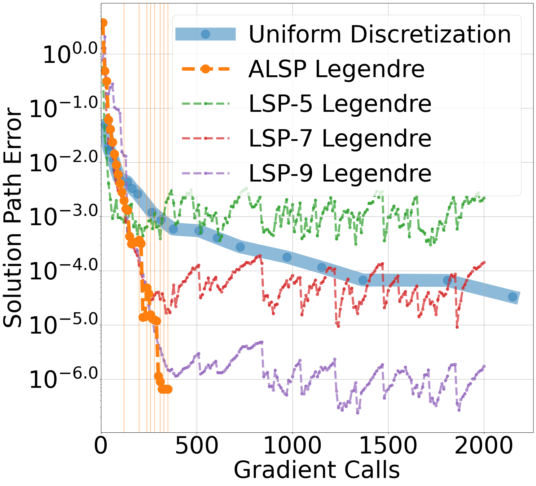
Figure 1: Learning Solution Path of Weighted Binary Classification. See Section 6 for setup. We compare our method with p=5,7,9𝑝579p=5,7,9 Legendre polynomials as our basis with uniform discretization. Orange line is our adaptive method (c.f. Algorithm 1). Vertical lines indicate when new basis functions are added.

Despite its simplicity, our approach can approximate the solution path to higher accuracy than discretization with fewer gradient evaluations. See Figure 1 for a sample of our numerical results on weighted binary classification using SGD to solve Equation 2. We prove this behavior is typical. Loosely,

  1. i)

    When using constant step-size SGD to solve Equation 2, we prove that the uniform error of our learned path 𝚽1:p(λ)𝜷^subscript𝚽:1𝑝𝜆^𝜷\boldsymbol{\Phi}_{1:p}(\lambda)\hat{\boldsymbol{\beta}} to the true path 𝜽(λ)superscript𝜽𝜆\boldsymbol{\theta}^{*}(\lambda) exhibits linear convergence to an irreducible constant that is proportional to the expressiveness of the basis (Theorem 3.4). This behavior is already visible in Figure 1.

The proof of this result utilizes ideas from the convergence of SGD under various “growth conditions” of the gradient (Bottou et al., 2018; Nguyen et al., 2018; Vaswani et al., 2019; Liu et al., 2024; Bertsekas, 1996). See Khaled and Richtárik (2020) for a summary and comparison of these various conditions. Our contribution to this literature is to relate the expressiveness of the basis Φ1:p(λ)subscriptΦ:1𝑝𝜆\Phi_{1:p}(\lambda) to a relaxed, weak-growth condition of Gower et al. (2019, Lemma 2.4). Indeed, we show that under some assumptions, Equation 2 always satisfies this relaxed weak-growth condition, and if the solution path lies in the span of the basis, it satisfies the weak-growth condition of Vaswani et al. (2019). This allows us to leverage results from those works to establish Theorem 3.4.

In special cases, we can leverage a priori knowledge of the structure of 𝜽(λ)superscript𝜽𝜆\boldsymbol{\theta}^{*}(\lambda) to prove stronger results. For example, suppose Λ=[1,1]Λ11\Lambda=[-1,1], and we use Legendre polynomials as our basis. We prove that

  1. ii)

    If the solution path 𝜽(λ)superscript𝜽𝜆\boldsymbol{\theta}^{*}(\lambda) is ν𝜈\nu-times differentiable, then using p=O(ϵ12(1ν))𝑝𝑂superscriptitalic-ϵ121𝜈p=O\left(\epsilon^{\frac{1}{2(1-\nu)}}\right) polynomials ensures that after T=O(ϵ11νlog(1/ϵ))𝑇𝑂superscriptitalic-ϵ11𝜈1italic-ϵT=O\left(\epsilon^{\frac{1}{1-\nu}}\log(1/\epsilon)\right) gradient calls, we obtain an ϵitalic-ϵ\epsilon-approximation to the solution path (Theorem 4.3).

For comparison, Ndiaye et al. (2019) implies that when h(𝜽,λ)𝜽𝜆h(\boldsymbol{\theta},\lambda) is strongly-convex, discretization requires at least O(ϵ1/2)𝑂superscriptitalic-ϵ12O(\epsilon^{-1/2}) points. Hence, even if the optimization problem at each grid point can be solved with 111 gradient evaluation, our approach requires asymptotically fewer evaluations whenever ν>3𝜈3\nu>3. If ν𝜈\nu is large, the savings is substantive.

  1. iii)

    If the solution path 𝜽(λ)superscript𝜽𝜆\boldsymbol{\theta}^{*}(\lambda) is analytic (ν=𝜈\nu=\infty), then using p=O(log(1/ϵ))𝑝𝑂1italic-ϵp=O(\log(1/\epsilon)) basis polynomials ensures that after T=O(log2(1/ϵ)loglog(1/ϵ))𝑇𝑂superscript21italic-ϵ1italic-ϵT=O(\log^{2}(1/\epsilon)\log\log(1/\epsilon)) iterations, we obtain an ϵitalic-ϵ\epsilon-approximation to the solution path (Theorem 4.5).

This is almost exponentially less work than discretization.

These specialized results strongly suggest that in the general setting our approach should be competitive as long as we use enough basis functions. This observation motivates a natural heuristic in which we adaptively add basis functions whenever the stochastic optimization routine (e.g., SGD) stalls (see Algorithm 1 and Section 5 for details). We illustrate this idea in Figure 1 (orange line) where we can see that by progressively adding functions we drive the uniform error to zero rapidly.

Algorithm 1 Adaptively Learn the Solution Path (ALSP)
1:  Initialize: 𝚽1:0()[]subscript𝚽:10\boldsymbol{\Phi}_{1:0}(\cdot)\leftarrow[\ ] and 𝜷^0[]subscript^𝜷0\hat{\boldsymbol{\beta}}_{0}\leftarrow[\ ]
2:  Return: A sequence of coefficients: 𝜷^1,𝜷^2,subscript^𝜷1subscript^𝜷2\hat{\boldsymbol{\beta}}_{1},\hat{\boldsymbol{\beta}}_{2},\ldots
3:  At iteration p=1,2,𝑝12p=1,2,\ldots do
4:   Append a new basis function:
𝚽1:p()[𝚽1:p1()𝚽p()]subscript𝚽:1𝑝delimited-[]subscript𝚽:1𝑝1subscript𝚽𝑝\boldsymbol{\Phi}_{1:p}(\cdot)\leftarrow\left[\boldsymbol{\Phi}_{1:{p-1}}(\cdot)\ \boldsymbol{\Phi}_{p}(\cdot)\right]
5:   Run a first-order method, starting from
6:   [𝜷^p1,0]psubscript^𝜷𝑝10superscript𝑝[\hat{\boldsymbol{\beta}}_{p-1},0]\in\mathbb{R}^{p}, to obtain
𝜷^pargmin𝜷p𝔼λ~λ[h(𝚽1:p(λ~)𝜷,λ~)].subscript^𝜷𝑝subscript𝜷superscript𝑝subscript𝔼similar-to~𝜆subscript𝜆delimited-[]subscript𝚽:1𝑝~𝜆𝜷~𝜆\hat{\boldsymbol{\beta}}_{p}~{}\approx~{}\arg\min_{\boldsymbol{\beta}\in\mathbb{R}^{p}}\ \mathbb{E}_{\tilde{\lambda}\sim\mathbb{P}_{\lambda}}\left[h(\boldsymbol{\Phi}_{1:p}(\tilde{\lambda})\boldsymbol{\beta},\tilde{\lambda})\right].

1.2 Other Related Work

There are some works that consider the total computational work to learn a solution path, typically focusing on a specific choice of h(,)h(\cdot,\cdot). See, e.g., Tibshirani (1996); Cortes and Vapnik (1995); Rosset (2004); Rosset and Zhu (2007); Friedman et al. (2010); Osborne et al. (2000); Hastie et al. (2004); Efron et al. (2004); Mairal and Yu (2012); Tibshirani and Taylor (2011); Ndiaye and Takeuchi (2021) for results on LASSO and regularized SVM; Park and Hastie (2007); Bao et al. (2019) for results on L1𝐿1L1-regularization. Liu and Grigas (2023) study a regularization path setting from an ordinary differential equations perspective using second-order methods. Overall, our work is similar to this larger stream in that we focus on total computational cost, but, unlike this stream, we develop a general-purpose framework with minimal assumptions on h(,)h(\cdot,\cdot).

2 Model Setup and Preliminaries

We denote the 2subscript2\ell_{2}-norm by \|\cdot\| throughout. We focus on the case of smooth, strongly convex functions:

Assumption 2.1 (Uniform Smoothness and Strong Convexity).

There are constants 0<μL0𝜇𝐿0<\mu\leq L such that, for all λΛ𝜆Λ\lambda\in\Lambda, h(,λ)𝜆h(\cdot,\lambda) is μ𝜇\mu-strongly convex and L𝐿L-smooth, i.e., for all 𝜽,𝜽¯d𝜽¯𝜽superscript𝑑\boldsymbol{\theta},\bar{\boldsymbol{\theta}}\in\mathbb{R}^{d},

μ2𝜽𝜽¯2h(𝜽)h(𝜽¯)h(𝜽¯)(𝜽𝜽¯)L2𝜽𝜽¯2.𝜇2superscriptnorm𝜽¯𝜽2𝜽¯𝜽superscript¯𝜽top𝜽¯𝜽𝐿2superscriptnorm𝜽¯𝜽2\frac{\mu}{2}\|\boldsymbol{\theta}-\bar{\boldsymbol{\theta}}\|^{2}~{}\leq~{}h(\boldsymbol{\theta})-h(\bar{\boldsymbol{\theta}})-\nabla h(\bar{\boldsymbol{\theta}})^{\top}(\boldsymbol{\theta}-\bar{\boldsymbol{\theta}})~{}\leq~{}\frac{L}{2}\|\boldsymbol{\theta}-\bar{\boldsymbol{\theta}}\|^{2}.

For any candidate solution path 𝜽()𝜽\boldsymbol{\theta}(\cdot), we define the solution path error of 𝜽()𝜽\boldsymbol{\theta}(\cdot) by

ϵsp(𝜽()):=supλΛ{h(𝜽(λ),λ)h(𝜽(λ),λ)}.assignsubscriptitalic-ϵsp𝜽subscriptsupremum𝜆Λ𝜽𝜆𝜆superscript𝜽𝜆𝜆\epsilon_{\rm sp}(\boldsymbol{\theta}(\cdot)):=\sup_{\lambda\in\Lambda}\left\{h(\boldsymbol{\theta}(\lambda),\lambda)-h(\boldsymbol{\theta}^{*}(\lambda),\lambda)\right\}.

An ϵitalic-ϵ\epsilon-solution path is a solution path 𝜽()𝜽\boldsymbol{\theta}(\cdot) such that ϵsp(𝜽())<ϵsubscriptitalic-ϵsp𝜽italic-ϵ\epsilon_{\rm sp}(\boldsymbol{\theta}(\cdot))<\epsilon. Finally, given any vector of coefficients 𝜷𝜷\boldsymbol{\beta} and basis functions 𝚽1:p()subscript𝚽:1𝑝\boldsymbol{\Phi}_{1:p}(\cdot), we define ϵsp(𝜷):=ϵsp(𝚽1:p()𝜷)assignsubscriptitalic-ϵsp𝜷subscriptitalic-ϵspsubscript𝚽:1𝑝𝜷\epsilon_{\rm sp}(\boldsymbol{\beta}):=\epsilon_{\rm sp}(\boldsymbol{\Phi}_{1:p}(\cdot)\boldsymbol{\beta}) to be the solution path error of 𝚽1:p()𝜷subscript𝚽:1𝑝𝜷\boldsymbol{\Phi}_{1:p}(\cdot)\boldsymbol{\beta}.

As mentioned, our method depends on two user-chosen parameters: a distribution λsubscript𝜆\mathbb{P}_{\lambda} over λΛ𝜆Λ\lambda\in\Lambda and a series of basis functions 𝚽j:Λd:subscript𝚽𝑗maps-toΛsuperscript𝑑\boldsymbol{\Phi}_{j}:\Lambda\mapsto\mathbb{R}^{d}, for j=1,,p𝑗1𝑝j=1,\ldots,p. We require some minor assumptions on these choices:

Assumption 2.2.

(Distribution, Basis Functions, and Linear Independence).

  1. i)

    It is easy to generate i.i.d. samples from λsubscript𝜆\mathbb{P}_{\lambda}.

  2. ii)

    It is easy to compute 𝚽j(λ)dsubscript𝚽𝑗𝜆superscript𝑑\boldsymbol{\Phi}_{j}(\lambda)\in\mathbb{R}^{d} for any λΛ𝜆Λ\lambda\in\Lambda, and 1jp1𝑗𝑝1\leq j\leq p.

  3. iii)

    There does not exist 𝜷p𝜷superscript𝑝\boldsymbol{\beta}\in\mathbb{R}^{p} with 𝜷0𝜷0\boldsymbol{\beta}\neq 0 such that 𝚽1:p(λ~)𝜷=𝟎subscript𝚽:1𝑝~𝜆𝜷0\boldsymbol{\Phi}_{1:p}(\tilde{\lambda})\boldsymbol{\beta}=\boldsymbol{0} holds λsubscript𝜆\mathbb{P}_{\lambda}-almost everywhere.

This last condition is a linear independence assumption. If violated, one can remove a function without affecting the span of the basis on the support of λsubscript𝜆\mathbb{P}_{\lambda}.

Given 𝚽1:psubscript𝚽:1𝑝\boldsymbol{\Phi}_{1:p}, we define the minimal solution path error for this basis by

ϵsp:=inf𝜷pϵsp(𝜷).assignsuperscriptsubscriptitalic-ϵspsubscriptinfimum𝜷superscript𝑝subscriptitalic-ϵsp𝜷\epsilon_{\rm sp}^{\ast}:=\inf_{\boldsymbol{\beta}\in\mathbb{R}^{p}}\epsilon_{\rm sp}(\boldsymbol{\beta}).

We also define the following auxiliary constants:

C𝐶\displaystyle C :=supλΛσmax(𝚽(λ)𝚽(λ)),assignabsentsubscriptsupremum𝜆Λsubscript𝜎𝚽superscript𝜆top𝚽𝜆\displaystyle~{}:=~{}\sup_{\lambda\in\Lambda}\sigma_{\max}\left(\boldsymbol{\Phi}(\lambda)^{\top}\boldsymbol{\Phi}(\lambda)\right), (3)
c𝑐\displaystyle c :=σmin{𝔼λ~λ[𝚽(λ~)𝚽(λ~)]}.assignabsentsubscript𝜎subscript𝔼similar-to~𝜆subscript𝜆delimited-[]𝚽superscript~𝜆top𝚽~𝜆\displaystyle~{}:=~{}\sigma_{\min}\left\{\mathbb{E}_{\tilde{\lambda}\sim\mathbb{P}_{\lambda}}\left[\boldsymbol{\Phi}(\tilde{\lambda})^{\top}\boldsymbol{\Phi}(\tilde{\lambda})\right]\right\}.

In words, C𝐶C is a uniform bound on the largest eigenvalue of the positive semidefinite matrix 𝚽(λ)𝚽(λ)𝚽superscript𝜆top𝚽𝜆\boldsymbol{\Phi}(\lambda)^{\top}\boldsymbol{\Phi}(\lambda), and c𝑐c is the smallest eigenvalue of the corresponding expected matrix. By construction, 0cC0𝑐𝐶0\leq c\leq C. Under Assumption 2.2, both constants are strictly positive.

Lemma 2.3 (Positive Spectral Values).

If Assumption 2.2 holds, then 0<cC0𝑐𝐶0<c\leq C.

We can now state our first key result which relates the suboptimality of a feasible solution 𝜷𝜷\boldsymbol{\beta} in Equation 2 to its solution path error. Define

𝜷avgargmin𝜷p𝔼λ~λ[h(𝚽(λ~)𝜷,λ~)].superscriptsubscript𝜷avgsubscript𝜷superscript𝑝subscript𝔼similar-to~𝜆subscript𝜆delimited-[]𝚽~𝜆𝜷~𝜆\boldsymbol{\beta}_{\mathrm{avg}}^{\ast}~{}\in~{}\arg\min_{\boldsymbol{\beta}\in\mathbb{R}^{p}}\ \mathbb{E}_{\tilde{\lambda}\sim\mathbb{P}_{\lambda}}\left[h(\boldsymbol{\Phi}(\tilde{\lambda})\boldsymbol{\beta},\tilde{\lambda})\right].
Theorem 2.4 (Relating Suboptimality to Solution Path Error).

Under Assumptions 2.2 and 2.1, for any 𝛃p𝛃superscript𝑝\boldsymbol{\beta}\in\mathbb{R}^{p}, we have

ϵsp(𝜷)2CL𝜷𝜷avg2+(8CLcμ)ϵsp.subscriptitalic-ϵsp𝜷2𝐶𝐿superscriptnorm𝜷superscriptsubscript𝜷avg28𝐶𝐿𝑐𝜇superscriptsubscriptitalic-ϵsp\epsilon_{\rm sp}(\boldsymbol{\beta})~{}\leq~{}2CL\|\boldsymbol{\beta}-\boldsymbol{\beta}_{\mathrm{avg}}^{\ast}\|^{2}+\left(\frac{8CL}{c\mu}\right)\epsilon_{\rm sp}^{\ast}.

This bound decomposes into two terms, one proportional to 𝜷𝜷avg2superscriptnorm𝜷superscriptsubscript𝜷avg2\|\boldsymbol{\beta}-\boldsymbol{\beta}_{\mathrm{avg}}^{\ast}\|^{2}, which represents the suboptimality of 𝜷𝜷\boldsymbol{\beta} and the other proportional to ϵspsuperscriptsubscriptitalic-ϵsp\epsilon_{\rm sp}^{\ast}, which measures the maximal expressiveness of the basis. By solving Equation 2 to greater accuracy, we can drive down the first term, but we will not affect the second term. To reduce the second term, we must add basis functions to obtain a better quality approximation.

Theorem 2.4 shows any algorithm for solving Equation 2 can be used to approximate the solution path. In the next section, we argue that when ϵspsuperscriptsubscriptitalic-ϵsp\epsilon_{\rm sp}^{\ast} is small, constant step-size SGD for Equation 2 exhibits linear convergence to a constant proportional to ϵspsuperscriptsubscriptitalic-ϵsp\epsilon_{\rm sp}^{*}, making it an ideal algorithm to study.

3 SGD to Learn the Solution Path

In this section, we apply constant step-size SGD to solve Equation 2. The key idea is to show that Equation 2 satisfies a certain growth condition and apply Gower et al. (2019, Theorem 3.1). One minor detail is that Gower et al. (2019) proves their result under a stronger “expected smoothness” condition for the setting where the objective Equation 2 is a finite sum. However, the result holds more generally under a weaker condition (Eq. (9) of their work). Hence, for clarity, we first restate this condition and the more general result.

The following definition is motivated by Gower et al. (2019, Lemma 2.4):

Definition 3.1 (Relaxed Weak Growth Condition (RWGC)).

Consider a family of functions g(,z):d:𝑔𝑧superscript𝑑g(\cdot,z):\mathbb{R}^{d}\to\mathbb{R}, zzsimilar-to𝑧subscript𝑧z\sim\mathbb{P}_{z}, and G():=𝔼zz[g(,z)]assign𝐺subscript𝔼similar-to𝑧subscript𝑧delimited-[]𝑔𝑧G(\cdot):=\mathbb{E}_{z\sim\mathbb{P}_{z}}\left[g(\cdot,z)\right]. Let G:=min𝒘dG(𝒘)assignsuperscript𝐺subscript𝒘superscript𝑑𝐺𝒘G^{*}:=\min_{\boldsymbol{w}\in\mathbb{R}^{d}}G(\boldsymbol{w}). Then, g𝑔g and G𝐺G are said to satisfy the relaxed weak growth condition with constants ρ0𝜌0\rho\geq 0 and σ0𝜎0\sigma\geq 0, if for all 𝒘d𝒘superscript𝑑\boldsymbol{w}\in\mathbb{R}^{d},

𝔼zz[g(𝒘,z)2]2ρ(G(𝒘)G)+σ2.subscript𝔼similar-to𝑧subscript𝑧delimited-[]superscriptnorm𝑔𝒘𝑧22𝜌𝐺𝒘superscript𝐺superscript𝜎2\mathbb{E}_{z\sim\mathbb{P}_{z}}\left[\|\nabla g(\boldsymbol{w},z)\|^{2}\right]~{}\leq~{}2\rho(G(\boldsymbol{w})-G^{*})+\sigma^{2}.

When σ=0𝜎0\sigma=0, Definition 3.1 recovers the weak growth condition of Vaswani et al. (2019). In this case, the variance of the stochastic gradients goes to zero as we approach an optimal solution. Hence, at optimality, not only is the expectation of the gradient zero, but it is zero almost surely in z𝑧z. For regression problems, this condition corresponds to interpolation.

Definition 3.1 is implied by a standard second moment condition on the gradients (take ρ=0𝜌0\rho=0). However, the most interesting cases are when σ2superscript𝜎2\sigma^{2} is small relative to ρ𝜌\rho and ρ>0𝜌0\rho>0. (This will be the case for Equation 2. See Section 3.1.)

We then have the following theorem.

Theorem 3.2 (Gower et al. (2019)).

Suppose that the RWGC holds for the family of functions g(,z):d:𝑔𝑧superscript𝑑g(\cdot,z):\mathbb{R}^{d}\to\mathbb{R}, and that G():=𝔼zz[g(,z)]assign𝐺subscript𝔼similar-to𝑧subscript𝑧delimited-[]𝑔𝑧G(\cdot):=\mathbb{E}_{z\sim\mathbb{P}_{z}}\left[g(\cdot,z)\right] is μgsubscript𝜇𝑔\mu_{g}-strongly convex for some for some μg>0subscript𝜇𝑔0\mu_{g}>0. Consider the SGD algorithm, initialized at 𝐰0dsubscript𝐰0superscript𝑑\boldsymbol{w}_{0}\in\mathbb{R}^{d}, with iterations

𝒘t+1=𝒘tη¯ρg(𝒘t,zt),subscript𝒘𝑡1subscript𝒘𝑡¯𝜂𝜌𝑔subscript𝒘𝑡subscript𝑧𝑡\boldsymbol{w}_{t+1}=\boldsymbol{w}_{t}-\frac{\bar{\eta}}{\rho}\nabla g(\boldsymbol{w}_{t},z_{t}),

where ztzsimilar-tosubscript𝑧𝑡subscript𝑧z_{t}\sim\mathbb{P}_{z} is a random sample and η¯(0,min{1,ρμg}]¯𝜂01𝜌subscript𝜇𝑔\bar{\eta}\in\left(0,\min\left\{1,\frac{\rho}{\mu_{g}}\right\}\right] parametrizes the step-size. Then for all t0𝑡0t\geq 0, we have

𝔼[𝒘t𝒘2](1η¯μgρ)t𝒘0𝒘2+η¯σ2ρμg.𝔼delimited-[]superscriptnormsubscript𝒘𝑡superscript𝒘2superscript1¯𝜂subscript𝜇𝑔𝜌𝑡superscriptnormsubscript𝒘0superscript𝒘2¯𝜂superscript𝜎2𝜌subscript𝜇𝑔\mathbb{E}[\|\boldsymbol{w}_{t}-\boldsymbol{w}^{*}\|^{2}]~{}\leq~{}\left(1-\frac{\bar{\eta}\mu_{g}}{\rho}\right)^{t}\|\boldsymbol{w}_{0}-\boldsymbol{w}^{*}\|^{2}+\frac{\bar{\eta}\sigma^{2}}{\rho\mu_{g}}.

In other words, constant step-size SGD under the RWGC exhibits a “fast” linear convergence in expectation up to a constant that is directly proportional to σ2superscript𝜎2\sigma^{2}, after which it stalls. When σ2=0superscript𝜎20\sigma^{2}=0, we exactly recover the result of Vaswani et al. (2019). To keep the exposition self-contained, we provide a proof in the appendix.

3.1 Solving Equation 2 with SGD

We next prove that Equation 2 satisfies RWGC, and in particular, that the “σ2superscript𝜎2\sigma^{2}” term depends on ϵspsuperscriptsubscriptitalic-ϵsp\epsilon_{\rm sp}^{\ast}, the minimal solution path error of the basis. To our knowledge, we are the first to make this observation.

Define

f(𝜷,λ)𝑓𝜷𝜆\displaystyle f(\boldsymbol{\beta},\lambda) :=h(𝚽(λ)𝜷,λ),assignabsent𝚽𝜆𝜷𝜆\displaystyle~{}:=~{}h(\boldsymbol{\Phi}(\lambda)\boldsymbol{\beta},\lambda), (4a)
F(𝜷)𝐹𝜷\displaystyle F(\boldsymbol{\beta}) :=𝔼λ~λ[f(𝜷,λ~)]assignabsentsubscript𝔼similar-to~𝜆subscript𝜆delimited-[]𝑓𝜷~𝜆\displaystyle~{}:=~{}\mathbb{E}_{\tilde{\lambda}\sim\mathbb{P}_{\lambda}}\left[f(\boldsymbol{\beta},\tilde{\lambda})\right]
=𝔼λ~λ[h(𝚽(λ~)𝜷,λ~)],absentsubscript𝔼similar-to~𝜆subscript𝜆delimited-[]𝚽~𝜆𝜷~𝜆\displaystyle~{}=~{}\mathbb{E}_{\tilde{\lambda}\sim\mathbb{P}_{\lambda}}\left[h(\boldsymbol{\Phi}(\tilde{\lambda})\boldsymbol{\beta},\tilde{\lambda})\right], (4b)
Lemma 3.3 (Equation 2 satisfies RWGC).

Suppose that Assumptions 2.2 and 2.1 hold and recall the constants defined in Equation 3. Then, the family of functions f(,λ)𝑓𝜆f(\cdot,\lambda) and the function F()𝐹F(\cdot), defined in Equation 4, satisfy the relaxed weak growth condition (RWGC) with constants ρ=CL𝜌𝐶𝐿\rho=CL and σ2=2CLϵspsuperscript𝜎22𝐶𝐿superscriptsubscriptitalic-ϵsp\sigma^{2}=2CL\epsilon_{\rm sp}^{\ast}. Namely, for all 𝛃d𝛃superscript𝑑\boldsymbol{\beta}\in\mathbb{R}^{d},

𝔼λ~λ[f(𝜷,λ~)2]2CL(F(𝜷)F)+2CLϵsp.subscript𝔼similar-to~𝜆subscript𝜆delimited-[]superscriptnorm𝑓𝜷~𝜆22𝐶𝐿𝐹𝜷superscript𝐹2𝐶𝐿superscriptsubscriptitalic-ϵsp\mathbb{E}_{\tilde{\lambda}\sim\mathbb{P}_{\lambda}}\left[\|\nabla f(\boldsymbol{\beta},\tilde{\lambda})\|^{2}\right]~{}\leq~{}2CL(F(\boldsymbol{\beta})-F^{*})+2CL\epsilon_{\rm sp}^{\ast}.

In addition, F()𝐹F(\cdot) is cμ𝑐𝜇c\mu-strongly convex.

We now combine Theorems 2.4, 3.2 and 3.3 to yield our main result: a bound on the expected solution path error for constant step-size SGD. Recall constant step-size SGD in this setting yields the iteration

𝜷t+1𝜷tη𝜷h(𝚽(λ~t)𝜷t,λ~t),subscript𝜷𝑡1subscript𝜷𝑡𝜂subscript𝜷𝚽subscript~𝜆𝑡subscript𝜷𝑡subscript~𝜆𝑡\boldsymbol{\beta}_{t+1}\leftarrow\boldsymbol{\beta}_{t}-\eta\nabla_{\boldsymbol{\beta}}h(\boldsymbol{\Phi}(\tilde{\lambda}_{t})\boldsymbol{\beta}_{t},\tilde{\lambda}_{t}),

where

𝜷h(𝚽(λ~t)𝜷t,λ~t)=𝚽(λ~t)𝜽h(𝚽(λ~t)𝜷t,λ~t),subscript𝜷𝚽subscript~𝜆𝑡subscript𝜷𝑡subscript~𝜆𝑡𝚽superscriptsubscript~𝜆𝑡topsubscript𝜽𝚽subscript~𝜆𝑡subscript𝜷𝑡subscript~𝜆𝑡\nabla_{\boldsymbol{\beta}}h(\boldsymbol{\Phi}(\tilde{\lambda}_{t})\boldsymbol{\beta}_{t},\tilde{\lambda}_{t})=\boldsymbol{\Phi}(\tilde{\lambda}_{t})^{\top}\nabla_{\boldsymbol{\theta}}h(\boldsymbol{\Phi}(\tilde{\lambda}_{t})\boldsymbol{\beta}_{t},\tilde{\lambda}_{t}),

and λ~tλsimilar-tosubscript~𝜆𝑡subscript𝜆\tilde{\lambda}_{t}\sim\mathbb{P}_{\lambda}. We assume that the gradient 𝜽h(𝜽,λ)subscript𝜽𝜽𝜆\nabla_{\boldsymbol{\theta}}h(\boldsymbol{\theta},\lambda) is easily computable for any 𝜽𝜽\boldsymbol{\theta} and λ𝜆\lambda.

We then have:

Theorem 3.4 (Expected Solution Path Error Convergence for SGD).

Under Assumptions 2.2 and 2.1, consider applying SGD to Equation 2 with a constant step-size η=η¯CL𝜂¯𝜂𝐶𝐿\eta=\frac{\bar{\eta}}{CL} parameterized by η¯(0,1]¯𝜂01\bar{\eta}\in\left(0,1\right]. Then, after T𝑇T iterations, the expected solution path error is at most

𝔼[ϵsp(𝜷T)]𝔼delimited-[]subscriptitalic-ϵspsubscript𝜷𝑇absent\displaystyle\mathbb{E}\left[\epsilon_{\rm sp}(\boldsymbol{\beta}_{T})\right]~{}\leq~{} 2CL𝜷0𝜷avg2(1η¯cμCL)T2𝐶𝐿superscriptnormsubscript𝜷0superscriptsubscript𝜷avg2superscript1¯𝜂𝑐𝜇𝐶𝐿𝑇\displaystyle 2CL\|\boldsymbol{\beta}_{0}-\boldsymbol{\beta}_{\mathrm{avg}}^{\ast}\|^{2}\left(1-\frac{\bar{\eta}c\mu}{CL}\right)^{T}
+(4CL(η¯+2)cμ)ϵsp.4𝐶𝐿¯𝜂2𝑐𝜇superscriptsubscriptitalic-ϵsp\displaystyle+\left(\frac{4CL(\bar{\eta}+2)}{c\mu}\right)\epsilon_{\rm sp}^{\ast}.

In particular, when ϵsp>0superscriptsubscriptitalic-ϵsp0\epsilon_{\rm sp}^{\ast}>0, then for TCLη¯cμlog(cμ𝛃0𝛃avg22η¯ϵsp)𝑇𝐶𝐿¯𝜂𝑐𝜇𝑐𝜇superscriptnormsubscript𝛃0superscriptsubscript𝛃avg22¯𝜂superscriptsubscriptitalic-ϵspT\geq\left\lceil\frac{CL}{\bar{\eta}c\mu}\log\left(\frac{c\mu\|\boldsymbol{\beta}_{0}-\boldsymbol{\beta}_{\mathrm{avg}}^{\ast}\|^{2}}{2\bar{\eta}\epsilon_{\rm sp}^{\ast}}\right)\right\rceil,

𝔼[ϵsp(𝜷T)](8CL(η¯+1)cμ)ϵsp.𝔼delimited-[]subscriptitalic-ϵspsubscript𝜷𝑇8𝐶𝐿¯𝜂1𝑐𝜇superscriptsubscriptitalic-ϵsp\mathbb{E}\left[\epsilon_{\rm sp}(\boldsymbol{\beta}_{T})\right]~{}\leq~{}\left(\frac{8CL(\bar{\eta}+1)}{c\mu}\right)\epsilon_{\rm sp}^{\ast}.

When ϵsp=0superscriptsubscriptitalic-ϵsp0\epsilon_{\rm sp}^{\ast}=0, then for any ϵ>0italic-ϵ0\epsilon>0 and TCLη¯cμlog(2CL𝛃0𝛃avg2ϵ)𝑇𝐶𝐿¯𝜂𝑐𝜇2𝐶𝐿superscriptnormsubscript𝛃0superscriptsubscript𝛃avg2italic-ϵT\geq\left\lceil\frac{CL}{\bar{\eta}c\mu}\log\left(\frac{2CL\|\boldsymbol{\beta}_{0}-\boldsymbol{\beta}_{\mathrm{avg}}^{\ast}\|^{2}}{\epsilon}\right)\right\rceil,

𝔼[ϵsp(𝜷T)]ϵ.𝔼delimited-[]subscriptitalic-ϵspsubscript𝜷𝑇italic-ϵ\mathbb{E}\left[\epsilon_{\rm sp}(\boldsymbol{\beta}_{T})\right]~{}\leq~{}\epsilon.

Theorem 3.4 highlights the role of the basis functions in our results. First we see that as T𝑇T\rightarrow\infty, the expected solution path error plateaus at a constant proportional to CLcμϵsp𝐶𝐿𝑐𝜇subscriptsuperscriptitalic-ϵsp\frac{CL}{c\mu}\epsilon^{\ast}_{\rm sp}. As mentioned, ϵspsubscriptsuperscriptitalic-ϵsp\epsilon^{\ast}_{\rm sp} measures the expressiveness of the basis, and we expect ϵspsuperscriptsubscriptitalic-ϵsp\epsilon_{\rm sp}^{*} to be small as we add more basis functions. We interpret CLcμ𝐶𝐿𝑐𝜇\frac{CL}{c\mu} as a condition number for Equation 2, which also depends on the choice of basis through Equation 3. This constant increases as we grow the basis. Finaly, the iteration complexity scales linearly with this condition number. Thus, an “ideal” basis must navigate this tradeoff between ϵspsubscriptsuperscriptitalic-ϵsp\epsilon^{\ast}_{\rm sp} and C/c𝐶𝑐C/c.

Fortunately, there exists a rich theory on function approximation that studies the relationship between basis functions, uniform error, and eigenspectra. In the next section we leverage this theory to provide a comparison of our method with existing discretization techniques in a specialized setting.

4 Specialized Results for Λ=[1,1]Λ11\Lambda=[-1,1]

We next leverage results from function approximation theory to bound the number of basis functions needed to achieve a target solution path error. We focus on the case Λ=[1,1]Λ11\Lambda=[-1,1] as it facilitates simple comparisons to existing results and elucidates key intuition.

We use a simple basis: we approximate each component i=1,,d𝑖1𝑑i=1,\ldots,d of θi()subscriptsuperscript𝜃𝑖\theta^{*}_{i}(\cdot) by the first q𝑞q Legendre polynomials. Hence the total number of basis functions is p=qd𝑝𝑞𝑑p=qd. Recall, the Legendre polynomials form an orthogonal basis on [1,1]11[-1,1] with respect to the uniform distribution, i.e., 𝔼λ~Unif[1,1][Pn(λ~)Pm(λ~)]=22n+1𝕀{n=m}subscript𝔼similar-to~𝜆Unif11delimited-[]subscript𝑃𝑛~𝜆subscript𝑃𝑚~𝜆22𝑛1𝕀𝑛𝑚\mathbb{E}_{\tilde{\lambda}\sim\text{Unif}[-1,1]}\left[P_{n}(\tilde{\lambda})P_{m}(\tilde{\lambda})\right]=\frac{2}{2n+1}\mathbb{I}\left\{n=m\right\}, where Pnsubscript𝑃𝑛P_{n} and Pmsubscript𝑃𝑚P_{m} are the nthsuperscript𝑛thn^{\text{th}} and mthsuperscript𝑚thm^{\text{th}} Legendre polynomial, respectively. Since we approximate each component separately, the matrix 𝚽(λ)d×qd𝚽𝜆superscript𝑑𝑞𝑑\boldsymbol{\Phi}(\lambda)\in\mathbb{R}^{d\times qd} is block-diagonal, with d blocks of size 1×q1𝑞1\times q.

For this basis, depending on the value of p=qd𝑝𝑞𝑑p=qd implied by the choice of q𝑞q, let Cp,cpsubscript𝐶𝑝subscript𝑐𝑝C_{p},c_{p} refer to the constants (3). We can bound the constant Cp/cpsubscript𝐶𝑝subscript𝑐𝑝C_{p}/c_{p}:

Lemma 4.1 (Cp/cpsubscript𝐶𝑝subscript𝑐𝑝C_{p}/c_{p} for Legendre Polynomials).

Take Λ=[1,1]Λ11\Lambda=[-1,1] and λsubscript𝜆\mathbb{P}_{\lambda} to be the uniform distribution on [1,1]11[-1,1]. Then, for the above basis, Cp/cpq2.subscript𝐶𝑝subscript𝑐𝑝superscript𝑞2C_{p}/c_{p}\leq q^{2}.

Notice, that this constant is independent of d𝑑d and grows mildly with q𝑞q. This is not true of all polynomial bases. One can check empirically that for the monomial basis, Cp/cpsubscript𝐶𝑝subscript𝑐𝑝C_{p}/c_{p} grows exponentially fast in q𝑞q.

Bounding ϵspsubscriptsuperscriptitalic-ϵsp\epsilon^{*}_{\rm sp} depends on the properties 𝜽(λ)superscript𝜽𝜆\boldsymbol{\theta}^{*}(\lambda). As a first example,

Lemma 4.2 (ϵspsubscriptsuperscriptitalic-ϵsp\epsilon^{*}_{\rm sp} for ν𝜈\nu-Differentiable Solution Paths).

Let Λ=[1,1]Λ11\Lambda=[-1,1]. Suppose Assumption 2.1 holds and that there exists an integer ν0𝜈0\nu\geq 0 and constant V>0𝑉0V>0 such that for all i=1,,d𝑖1𝑑i=1,\ldots,d, θi(λ)subscriptsuperscript𝜃𝑖𝜆\theta^{*}_{i}(\lambda) has ν𝜈\nu derivatives and the νthsuperscript𝜈th\nu^{\text{th}} derivative 𝛉i(ν)superscriptsubscript𝛉𝑖absent𝜈\boldsymbol{\theta}_{i}^{\ast(\nu)} is V𝑉V-Lipschitz continuous. Then, for any qν+1𝑞𝜈1q\geq\nu+1, for the basis described above, ϵspdL2(2Vπν(qν)ν)2.subscriptsuperscriptitalic-ϵsp𝑑𝐿2superscript2𝑉𝜋𝜈superscript𝑞𝜈𝜈2\epsilon^{*}_{\rm sp}\ \leq\ \frac{dL}{2}\left(\frac{2V}{\pi\nu(q-\nu)^{\nu}}\right)^{2}.

The proof of Lemma 4.2 is constructive; we exhibit a polynomial with the given solution path error.

Combining these lemmas with Theorem 3.4 allows us to calculate the requisite basis size and number of iterations needed to achieve a target solution-path error:

Theorem 4.3 (SGD for ν𝜈\nu-differentiable Solution Paths).

Let Λ=[1,1]Λ11\Lambda=[-1,1], λsubscript𝜆\mathbb{P}_{\lambda} be the uniform distribution on [1,1]11[-1,1]. Then, under the conditions of Lemma 4.2, if we use q=O(ϵ12(1ν))𝑞𝑂superscriptitalic-ϵ121𝜈q=O(\epsilon^{\frac{1}{2(1-\nu)}}) polynomials in the previous basis, and run constant-step size SGD for O(ϵ11νlog(1/ϵ))𝑂superscriptitalic-ϵ11𝜈1italic-ϵO(\epsilon^{\frac{1}{1-\nu}}\log(1/\epsilon)) iterations, the resulting iterate 𝛃Tsubscript𝛃𝑇\boldsymbol{\beta}_{T} satisfies 𝔼[ϵsp(𝛃T)]ϵ𝔼delimited-[]subscriptitalic-ϵspsubscript𝛃𝑇italic-ϵ\mathbb{E}\left[\epsilon_{\rm sp}(\boldsymbol{\beta}_{T})\right]\leq\epsilon.

For clarity, both big “Oh” terms should be interpreted as ϵ0italic-ϵ0\epsilon\rightarrow 0, and both suppress constants not depending on ϵitalic-ϵ\epsilon (but possibly depending on hh). Loosely, the theorem establishes that the “smoother” 𝜽()superscript𝜽\boldsymbol{\theta}^{*}(\cdot) is (i.e. larger ν𝜈\nu), the fewer iterations required by our method to achieve a target tolerance.

Recall, Ndiaye et al. (2019) established that for strongly convex functions, discretization requires at least O(ϵ1/2)𝑂superscriptitalic-ϵ12O(\epsilon^{-1/2}) points. One might expect the number of gradient evaluations per point to scale like O(log(1/ϵ))𝑂1italic-ϵO(\log(1/\epsilon)). Hence, if ν3𝜈3\nu\geq 3, our approach requires asymptotically less work. The larger ν𝜈\nu, the larger the savings.

This gap is particularly striking ν𝜈\nu\rightarrow\infty. As a second example, suppose θi(λ)subscriptsuperscript𝜃𝑖𝜆\theta^{*}_{i}(\lambda) is analytic on [1,1]11[-1,1], i.e, its Taylor Series is absolutely convergent on this interval.

Lemma 4.4 (ϵspsubscriptsuperscriptitalic-ϵsp\epsilon^{*}_{\rm sp} for Analytic Solution Paths).

Suppose Assumption 2.1 holds and that for each i=1,,d𝑖1𝑑i=1,\ldots,d, θi()subscriptsuperscript𝜃𝑖\theta^{*}_{i}(\cdot) is analytic on the interval [1,1]11[-1,1]. Then, there exist constants ω>1𝜔1\omega>1 and M>0𝑀0M>0 such that for any q>0𝑞0q>0, with the basis described above, ϵspdL2(2Mωqω1)2.subscriptsuperscriptitalic-ϵsp𝑑𝐿2superscript2𝑀superscript𝜔𝑞𝜔12\epsilon^{*}_{\rm sp}\leq\frac{dL}{2}\left(\frac{2M\omega^{-q}}{\omega-1}\right)^{2}.

The proof is again constructive. The constants ω𝜔\omega and M𝑀M pertain to the analytic continuation of θi()subscriptsuperscript𝜃𝑖\theta^{*}_{i}(\cdot) to the complex plane. Importantly, the solution path error now dies geometrically fast (like ω2qsuperscript𝜔2𝑞\omega^{-2q}). Using this faster decay rate yields,

Theorem 4.5 (SGD for Analytic Solution Paths).

Let Λ=[1,1]Λ11\Lambda=[-1,1], and λsubscript𝜆\mathbb{P}_{\lambda} be the uniform distribution on [1,1]11[-1,1]. Then, under the conditions of Lemma 4.4, if we use q=log(1/ϵ)/log(ω)𝑞1italic-ϵ𝜔q=\log(1/\epsilon)/\log(\omega) polynomials in the previous basis, and run constant-step size SGD for O(log2(1/ϵ)loglog(1/ϵ))𝑂superscript21italic-ϵ1italic-ϵO\left(\log^{2}(1/\epsilon)\log\log(1/\epsilon)\right) iterations, the resulting iterate 𝛃Tsubscript𝛃𝑇\boldsymbol{\beta}_{T} satisfies 𝔼[ϵsp(𝛃T)]ϵ𝔼delimited-[]subscriptitalic-ϵspsubscript𝛃𝑇italic-ϵ\mathbb{E}\left[\epsilon_{\rm sp}(\boldsymbol{\beta}_{T})\right]\leq\epsilon.

Again, the big “Oh” hides constants that do not depend on ϵitalic-ϵ\epsilon. Compared to Ndiaye et al. (2019), the amount of work almost exponentially smaller.

5 An Adaptive Algorithm

Although the previous section’s specialized results provide theoretical insight, they do not suggest practical algorithms. Picking the number of basis apriori from approximation theory is difficult. This challenge motivates our algorithm Algorithm 1, where the number of basis functions is determined “on the fly.” To implement Algorithm 1, one needs to specify i) a sequence of basis functions ii) a distribution λsubscript𝜆\mathbb{P}_{\lambda} and iii) a criterion for deciding when to add a new basis function. We next discuss these choices.

Although any basis and distribution can be used in Algorithm 1, we suggest making these choices in concert. In our experiments we focus on sequences of polynomials that are orthogonal with respect to λsubscript𝜆\mathbb{P}_{\lambda}. The Legendre polynomials and the uniform distribution on [1,1]11[-1,1] is one such pair, but there are many canonical examples including Hermite polynomials with the normal distribution and Laguerre polynomials with the exponential distribution. There are performance-optimized implementations of these families in standard software (see, e.g., scipy.special). Although polynomials map to \mathbb{R}, by approximating each dimension separately as in Section 4, we can extend these polynomials to a basis for d>1𝑑1d>1. Finally, polynomials are uniform function approximators for Lipschitz functions. Thus, the class is highly expressive.

Two other advantages of orthogonal polynomials in Algorithm 1 are: i) Extending the basis does not require altering existing basis functions. This is unlike, e.g., cubic splines or adding nodes to a neural network, where the addition of a new spline point affects previous bases. ii) Intuitively, orthogonality suggests that if 𝜷^p1subscript^𝜷𝑝1\hat{\boldsymbol{\beta}}_{p-1} is near optimal in the (p1)thsuperscript𝑝1th(p-1)^{\text{th}} iteration, then [𝜷^p1,0]subscript^𝜷𝑝10[\hat{\boldsymbol{\beta}}_{p-1},0] is likely to be close to optimal in the pthsuperscript𝑝thp^{\text{th}} iteration. Thus, we benefit from warmstarts.

We next discuss the criterion for adding a new basis function. One approach is to empirically approximate the objective of Equation 2 using a hold-out validation set, and add a basis function when performance stalls. This approach requires additional functional evaluations and samples λ~~𝜆\tilde{\lambda}. In our experiments, we explore an alternate criterion motivated by the RWGC. Specifically, if 𝜷𝜷\boldsymbol{\beta} is near-optimal, the upperbound on the second moment of the gradient in RWGC is approximately constant. Thus, we add a basis function when second moment of the gradient averaged over recent iterations has plateaued. This allows us to reuse gradients and additional function evaluations.

6 Numerical Experiments

We next empirically compare i) our approach using a fixed, large basis (denoted LSP for “Learning the Solution Path”) ii) our adaptive Algorithm 1 (denoted ALSP for “Adaptive LSP” and iii) uniform discretization, a natural benchmark. We aim to show that both our approaches not only outperform the benchmark but that the qualitative insights from our theoretical results hold for more general optimization procedures than constant step-size SGD. We also provide preliminary results on how the choice of basis affects performance.

We choose uniform discretization for our benchmark in lieu of other schemes (like geometric spacing) because i) it matches the theoretical lower bound from (Ndiaye et al., 2019) and ii) we see it as most intuitive for learning the solution path with small uniform error. Specifically, for various ϵitalic-ϵ\epsilon, we consider a uniform spacing of size ϵitalic-ϵ\sqrt{\epsilon} in each dimension of λ𝜆\lambda, and run (warm-started) gradient descent for O(log(1/ϵ))𝑂1italic-ϵO(\log(1/\epsilon)) iterations. The constant here is calibrated in an oracle fashion to achieve a solution-path error of O(ϵ)𝑂italic-ϵO(\epsilon) (see Section B.1 for details) giving the benchmark a small advantage.

6.1 Weighted Binary Classification

We consider a binary classification problem using a randomly selected subset of 100010001000 cases from the highly imbalanced Law School Admission Bar Passage dataset (Wightman, 1998). Of the 100010001000 cases, there are 956956956 positive instances and 444444 negatives. Standard logistic regression predicts 992992992 positives with a false positive rate of 0.860.860.86. When identifying students likely to fail is key, the default classifier may not be useful. Reweighting cases is a standard approach to improve false positive rate at the cost of overall accuracy.

We take

h(𝜽,λ)=(1λ)lpos(𝜽)+λlneg(𝜽)+0.125𝜽2,𝜽𝜆1𝜆subscript𝑙pos𝜽𝜆subscript𝑙neg𝜽0.125superscriptnorm𝜽2h(\boldsymbol{\theta},\lambda)=(1-\lambda)l_{\text{pos}}(\boldsymbol{\theta})+\lambda l_{\text{neg}}(\boldsymbol{\theta})+0.125\|\boldsymbol{\theta}\|^{2},

where lpos(𝜽)subscript𝑙pos𝜽l_{\text{pos}}(\boldsymbol{\theta}) and lneg(𝜽)subscript𝑙neg𝜽l_{\text{neg}}(\boldsymbol{\theta}) denote the log-likelihood on the positive and negative classes respectively. Specifically, letting (𝒙i,yi)45×{0,1}subscript𝒙𝑖subscript𝑦𝑖superscript4501(\boldsymbol{x}_{i},y_{i})\in\mathbb{R}^{45}\times\{0,1\} for i=1,,n𝑖1𝑛i=1,\ldots,n denote the data,

lpos(𝜽)=1|{i:yi=1}|i:yi=1log(1+e(2yi+1)𝒙i𝜽),subscript𝑙pos𝜽1conditional-set𝑖subscript𝑦𝑖1subscript:𝑖subscript𝑦𝑖11superscript𝑒2subscript𝑦𝑖1superscriptsubscript𝒙𝑖top𝜽l_{\text{pos}}(\boldsymbol{\theta})=\frac{1}{|\{i:\ y_{i}=1\}|}\sum_{i:y_{i}=1}\log(1+e^{(-2y_{i}+1)\boldsymbol{x}_{i}^{\top}\boldsymbol{\theta}}),

and similarly for lneg(𝜽)subscript𝑙neg𝜽l_{\text{neg}}(\boldsymbol{\theta}).

The hyperparameter λ[0,1]𝜆01\lambda\in[0,1] controls the weight placed on each class. We use (scaled and shifted) Legendre polynomials with a Unif[0,1]Unif01\text{Unif}[0,1] distribution.

The ground truth 𝜽(λ)superscript𝜽𝜆\boldsymbol{\theta}^{*}(\lambda) is computed via 500050005000 iterations of (warm-started) gradient descent over a uniform grid of 210superscript2102^{10} points. Solution path error is approximated by the uniform error over this grid.

For LSP, we run SGD using torch.optim.SGD. In lieu of a constant learning rate, we dynamically reduce the learning rate according to the Distance Diagnostic of Pesme et al. (2020, Section 4). This dynamic updating is more reflective of practice. We use the suggested parameters from Pesme et al. (2020) with the exception of q𝑞q, which we tune by examining the performance after 200200200 iterations. (We take q=1.3𝑞1.3q=1.3) For ALSP, we initialize the algorithm with 555 polynomials and stop it after adding 121212 polynomials.

Refer to caption
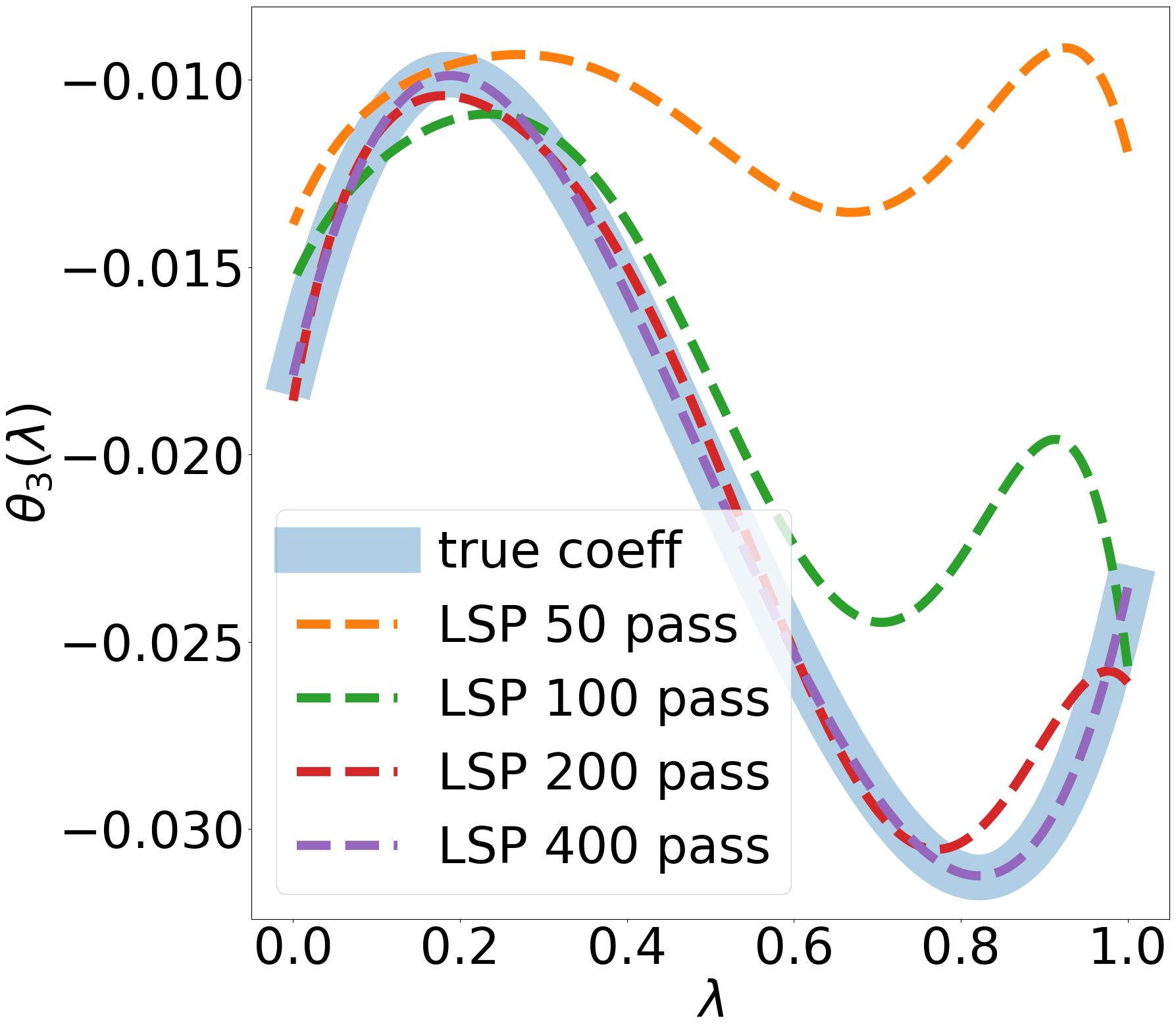
Figure 2: LSP: Interpolating the Solution Path for Weighted Binary Classification. Compare 𝚽3,1:7(λ)𝜷^subscript𝚽:317𝜆bold-^𝜷\boldsymbol{\Phi}_{3,1:7}(\lambda)\boldsymbol{\hat{\beta}} to 𝜽3(λ)subscriptsuperscript𝜽3𝜆\boldsymbol{\theta}^{\ast}_{3}(\lambda) across λ𝜆\lambda after running LSP with 777 Legendre polynomials for 500, 100, 200, 400 gradient calls.

Figure 1 in the introduction shows the performance for LSP. As we can see, LSP methods converge rapidly to an irreducible error, and this error decreases as we add basis functions. Our adaptive method converges rapidly. This performance is resonated by Figure 2, where we plot the coefficient profile for θ3(λ)subscriptsuperscript𝜃3𝜆\theta^{*}_{3}(\lambda) when using 777 polynomials. The approximation improves as we increase the number of iterations, and eventually become closely aligned with the true solution path.

Practically, this experiment suggests that when the region of ΛΛ\Lambda is compact, taking λsubscript𝜆\mathbb{P}_{\lambda} to be uniform paired with a polynomial basis is favorable. The polynomial basis can then be taken to be orthogonal to λsubscript𝜆\mathbb{P}_{\lambda} as discussed in Section 5.

6.2 Portfolio Allocation

We next consider a portfolio allocation problem calibrated to real data where 𝜽d𝜽superscript𝑑\boldsymbol{\theta}\in\mathbb{R}^{d} represents the weights on d=10𝑑10d=10 different asset classes. Namely, let μd𝜇superscript𝑑\mu\in\mathbb{R}^{d} and Σd×dΣsuperscript𝑑𝑑\Sigma\in\mathbb{R}^{d\times d} be the mean and covariance matrix of the returns of the different asset classes. We fit these parameters to the monthly return data from Aug. 2014 to July 2024 using the Fama-French 10 Industry index dataset.111https://mba.tuck.dartmouth.edu/pages/faculty/ken.french/data_library.html

We then solve

min𝜽subscript𝜽\displaystyle\min_{\boldsymbol{\theta}} λ1μ𝜽+λ2𝜽Σ𝜽+¯1(𝜽).subscript𝜆1superscript𝜇top𝜽subscript𝜆2superscript𝜽topΣ𝜽subscript¯1𝜽\displaystyle\quad-\lambda_{1}\mu^{\top}\boldsymbol{\theta}+\lambda_{2}\boldsymbol{\theta}^{\top}\Sigma\boldsymbol{\theta}+\bar{\ell}_{1}(\boldsymbol{\theta}).

Here the first term represents the (negative) expected return, the second represents the risk (variance) and the third is a smoothed version 1subscript1\ell_{1} regularization to induce sparsity. Namely, ¯1(𝜽):=i=1dθi2+.012.01.assignsubscript¯1𝜽superscriptsubscript𝑖1𝑑superscriptsubscript𝜃𝑖2superscript.012.01\bar{\ell}_{1}(\boldsymbol{\theta}):=\sum_{i=1}^{d}\sqrt{\theta_{i}^{2}+.01^{2}}-.01. The parameters λ1[0,1]subscript𝜆101\lambda_{1}\in[0,1] and λ2[0.2,1]subscript𝜆20.21\lambda_{2}\in[0.2,1] control the tradeoffs in these multiple objectives.

Ground truth 𝜽(λ)superscript𝜽𝜆\boldsymbol{\theta}^{*}(\lambda) is computed over a 100×100100100100\times 100 grid.

We focus on bivariate-Legendre polynomials for our basis, scaled and shifted to be orthogonal to uniform distribution on [0,1]×[.2,1]01.21[0,1]\times[.2,1]. We initialize with ALSP with 2 polynomials in each dimension, and iterate by adding one polynomial in each dimension, so that p=4,9,16,25𝑝491625p=4,9,16,25, after which we stop.

Unlike our previous experiment, to showcase that the qualitative insights of our theory hold for other algorithms other than SGD, we use torch.optim.BFGS for LSP, ALSP and uniform discretization (for a fair comparison). Unlike SGD, BFGS uses both function and gradient evaluations. We restrict it to use only 101010 function calls per gradient step so that the total work is still proportional to number of gradient calls.
Refer to caption
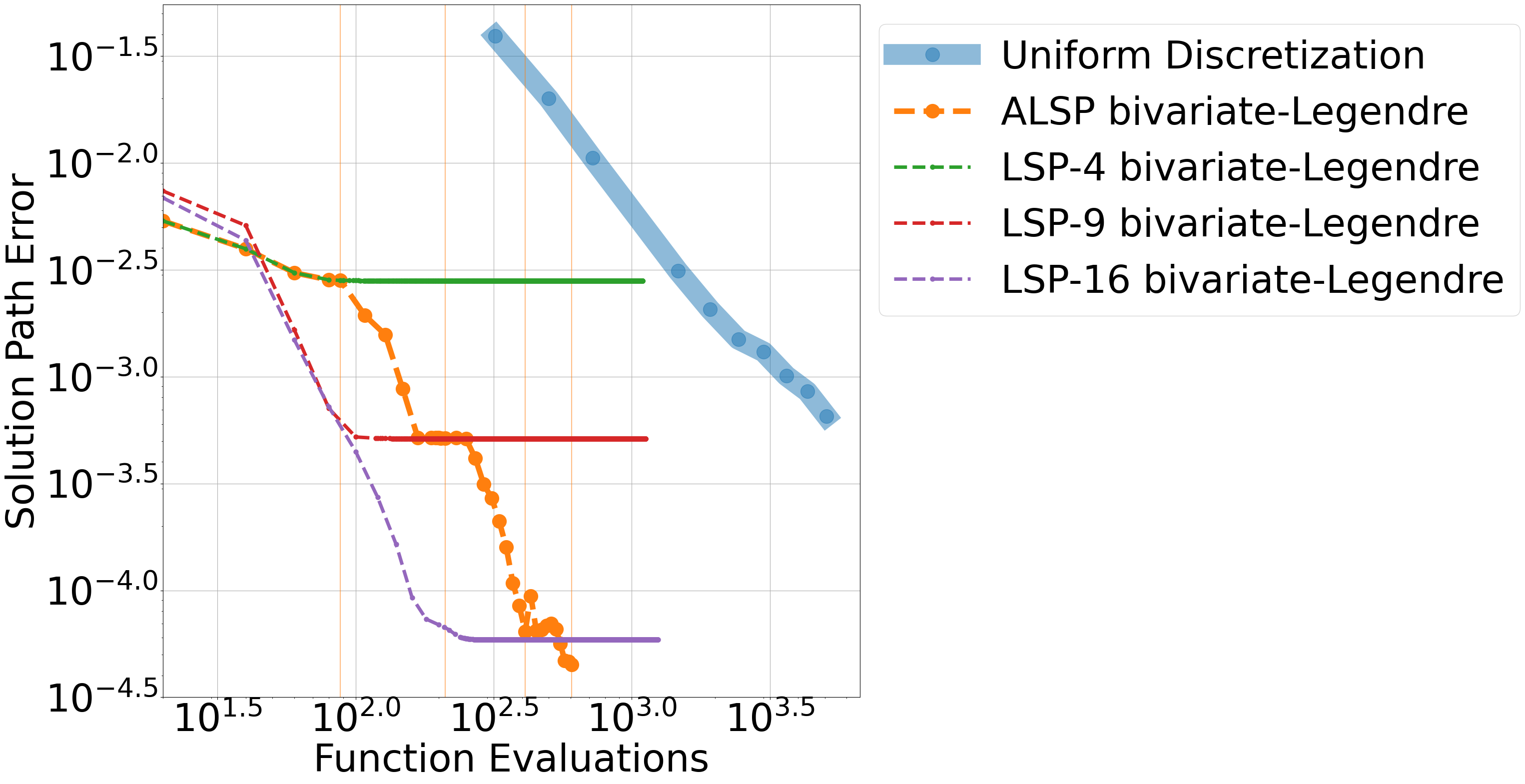
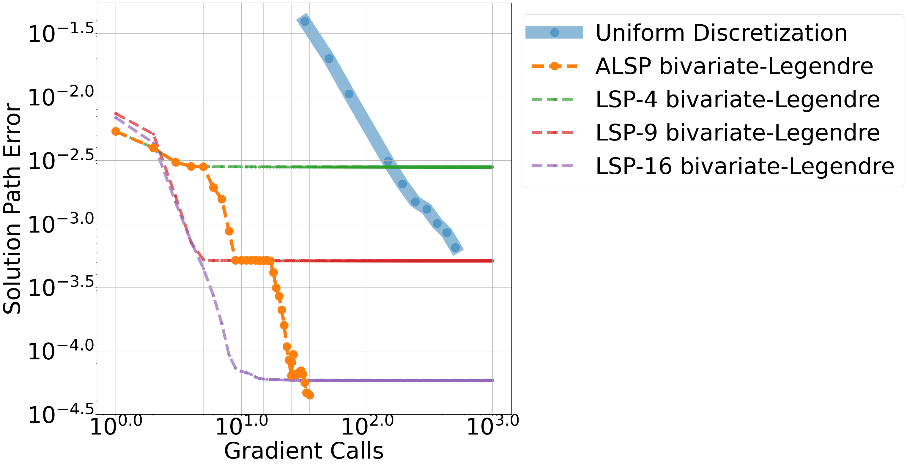
Figure 3: LSP and ALSP for Portfolio Allocation. Compares methods using the first p=4,9,16𝑝4916p=4,9,16 bivariate-Legendre polynomials.

As in our previous experiment, we see that LSP rapidly converges to an irreducible error and then plateaus. By contrast, ALSP seems to make continued progress as we add polynomials. Both method substantively outperform uniform discretization.

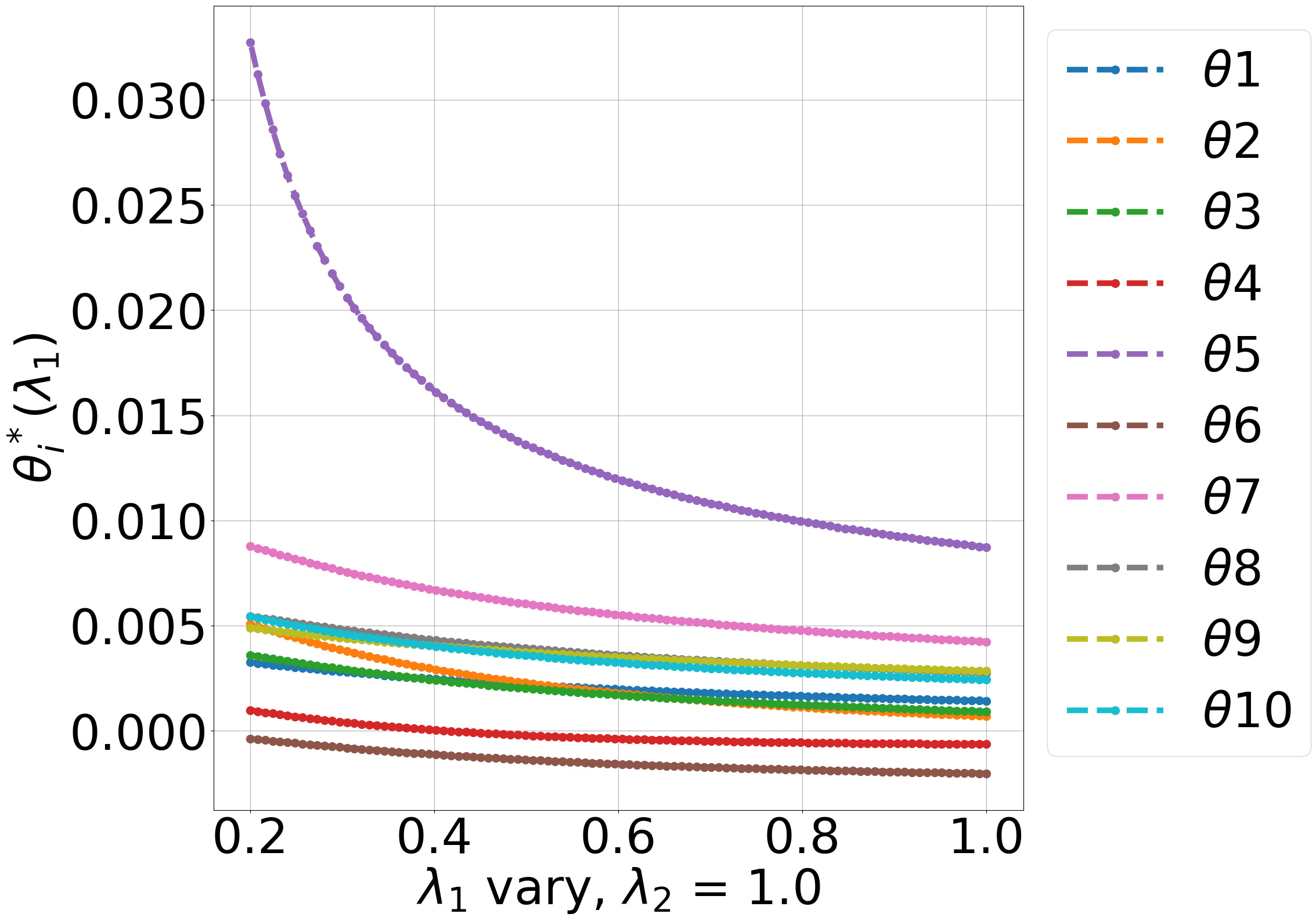
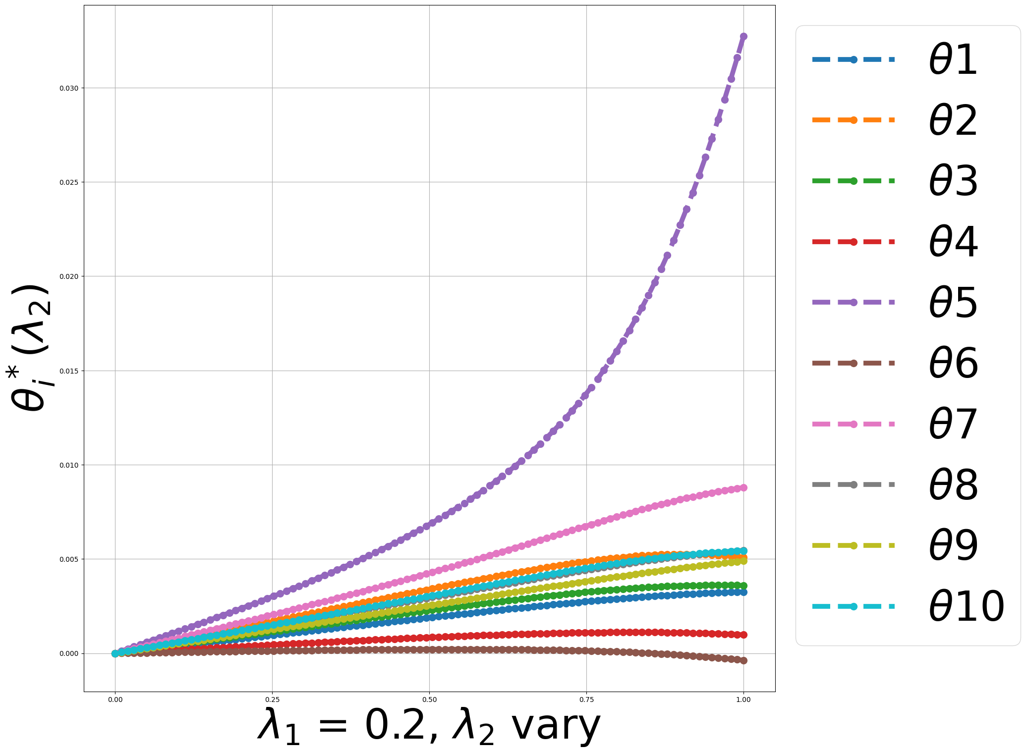
The improved performance over uniform discretization is partially attributable to the increased dimension of ΛΛ\Lambda (because discretization suffers the curse of dimensionality), but is also because (traditionally) discretization interpolates solutions in a piecewise constant fashion. In this example, 𝜽(λ)superscript𝜽𝜆\boldsymbol{\theta}^{*}(\lambda) is very smooth. See Figure 5 in Appendix. Hence, polynomial can learn to interpolate values very fast, while uniform discretization needs a great deal more resolution.

7 Conclusion

We propose a new method for learning the optimal solution path of a family of problems by reframing it as a single stochastic optimization problem over a linear combination of pre-specified basis functions. Compared to discretization schemes, our method offers flexibility and scalability by taking a global perspective on the solution path. When using sufficiently large bases, we prove our problem satisfies a certain relaxed weak-growth condition that strongly allows us to solve the single optimization problm very efficiently. Theoretical results in special cases and numerical experiments in more general settings support these findings.

Future research might more carefully examine the interplay between the parameterization of the family of problems and choice of basis. One might also consider other universal function approximators (like deep neural networks or forests of trees) within this context.

References

  • Bao et al. (2019) R. Bao, B. Gu, and H. Huang. Efficient approximate solution path algorithm for order weight l_1-norm with accuracy guarantee. In 2019 IEEE International Conference on Data Mining (ICDM), pages 958–963. IEEE, 2019.
  • Bertsekas (1996) D. Bertsekas. Neuro-dynamic programming. Athena Scientific, 1996.
  • Bottou et al. (2018) L. Bottou, F. E. Curtis, and J. Nocedal. Optimization methods for large-scale machine learning. SIAM review, 60(2):223–311, 2018.
  • Cortes and Vapnik (1995) C. Cortes and V. Vapnik. Support-vector networks. Machine Learning, 20:273–297, 1995.
  • Efron et al. (2004) B. Efron, T. Hastie, I. Johnstone, and R. Tibshirani. Least angle regression. 2004.
  • Friedman et al. (2010) J. Friedman, T. Hastie, and R. Tibshirani. Regularization paths for generalized linear models via coordinate descent. Journal of Statistical Software, 33(1):1, 2010.
  • Giesen et al. (2010) J. Giesen, M. Jaggi, and S. Laue. Approximating parameterized convex optimization problems. pages 524–535, 09 2010. ISBN 978-3-642-15774-5. doi: 10.1007/978-3-642-15775-2“˙45.
  • Giesen et al. (2012) J. Giesen, S. Laue, J. Mueller, and S. Swiercy. Approximating concavely parameterized optimization problems. Advances in Neural Information Processing Systems, 3:2105–2113, 01 2012.
  • Gower et al. (2019) R. M. Gower, N. Loizou, X. Qian, A. Sailanbayev, E. Shulgin, and P. Richtárik. Sgd: General analysis and improved rates. In International conference on machine learning, pages 5200–5209. PMLR, 2019.
  • Gupta et al. (2023) S. Gupta, J. Moondra, and M. Singh. Which lp norm is the fairest? approximations for fair facility location across all” p”. In Proceedings of the 24th ACM Conference on Economics and Computation, pages 817–817, 2023.
  • Hastie et al. (2004) T. Hastie, S. Rosset, R. Tibshirani, and J. Zhu. The entire regularization path for the support vector machine. Journal of Machine Learning Research, 5(Oct):1391–1415, 2004.
  • Khaled and Richtárik (2020) A. Khaled and P. Richtárik. Better theory for sgd in the nonconvex world. arXiv preprint arXiv:2002.03329, 2020.
  • Lan (2020) G. Lan. First-order and Stochastic Optimization Methods for Machine Learning, volume 1. Springer, 2020.
  • Liu et al. (2024) C. Liu, D. Drusvyatskiy, M. Belkin, D. Davis, and Y. Ma. Aiming towards the minimizers: fast convergence of sgd for overparametrized problems. Advances in neural information processing systems, 36, 2024.
  • Liu and Grigas (2023) H. Liu and P. Grigas. New methods for parametric optimization via differential equations. arXiv preprint arXiv:2306.08812, 2023.
  • Mairal and Yu (2012) J. Mairal and B. Yu. Complexity analysis of the lasso regularization path. In Proceedings of the 29th International Coference on International Conference on Machine Learning, pages 1835–1842, 2012.
  • Ndiaye and Takeuchi (2021) E. Ndiaye and I. Takeuchi. Continuation path with linear convergence rate. arXiv preprint arXiv:2112.05104, 2021.
  • Ndiaye et al. (2019) E. Ndiaye, T. Le, O. Fercoq, J. Salmon, and I. Takeuchi. Safe grid search with optimal complexity. In International Conference on Machine Learning, pages 4771–4780. PMLR, 2019.
  • Nguyen et al. (2018) L. Nguyen, P. H. Nguyen, M. Dijk, P. Richtárik, K. Scheinberg, and M. Takác. Sgd and hogwild! convergence without the bounded gradients assumption. In International Conference on Machine Learning, pages 3750–3758. PMLR, 2018.
  • Osborne et al. (2000) M. R. Osborne, B. Presnell, and B. A. Turlach. A new approach to variable selection in least squares problems. IMA Journal of Numerical Analysis, 20(3):389–403, 2000.
  • Park and Hastie (2007) M. Y. Park and T. Hastie. L1-Regularization Path Algorithm for Generalized Linear Models. Journal of the Royal Statistical Society Series B: Statistical Methodology, 69(4):659–677, 08 2007. ISSN 1369-7412.
  • Pesme et al. (2020) S. Pesme, A. Dieuleveut, and N. Flammarion. On convergence-diagnostic based step sizes for stochastic gradient descent. In International Conference on Machine Learning, pages 7641–7651. PMLR, 2020.
  • Rosset (2004) S. Rosset. Following curved regularized optimization solution paths. Advances in Neural Information Processing Systems, 17, 2004.
  • Rosset and Zhu (2007) S. Rosset and J. Zhu. Piecewise linear regularized solution paths. The Annals of Statistics, pages 1012–1030, 2007.
  • Tibshirani (1996) R. Tibshirani. Regression shrinkage and selection via the lasso. Journal of the Royal Statistical Society Series B: Statistical Methodology, 58(1):267–288, 1996.
  • Tibshirani and Taylor (2011) R. J. Tibshirani and J. Taylor. The solution path of the generalized lasso. The Annals of Statistics, 39(3):1335 – 1371, 2011. doi: 10.1214/11-AOS878. URL https://doi.org/10.1214/11-AOS878.
  • Trefethen (2013) L. N. Trefethen. Approximation Theory and Approximation Practice. SIAM, 2013.
  • Vaswani et al. (2019) S. Vaswani, F. Bach, and M. Schmidt. Fast and faster convergence of sgd for over-parameterized models and an accelerated perceptron. In The 22nd International Conference on Artificial Intelligence and Statistics, pages 1195–1204. PMLR, 2019.
  • Wightman (1998) L. F. Wightman. Lsac national longitudinal bar passage study. lsac research report series. 1998.

Appendix A Omitted Proofs

A.1 Proofs from Section 2

Proof for Lemma 2.3..

Suppose by contradiction that c=0𝑐0c=0. Then there exists a corresponding eigenvector 𝒗p𝒗superscript𝑝\boldsymbol{v}\in\mathbb{R}^{p} with 𝒗𝟎𝒗0\boldsymbol{v}\neq\boldsymbol{0} such that

𝔼λ~λ[𝚽(λ~)𝚽(λ~)]𝒗=𝟎𝔼λ~λ[𝚽(λ~)𝒗22]=0.subscript𝔼similar-to~𝜆subscript𝜆delimited-[]𝚽superscript~𝜆top𝚽~𝜆𝒗0subscript𝔼similar-to~𝜆subscript𝜆delimited-[]subscriptsuperscriptnorm𝚽~𝜆𝒗220\mathbb{E}_{\tilde{\lambda}\sim\mathbb{P}_{\lambda}}\left[\boldsymbol{\Phi}(\tilde{\lambda})^{\top}\boldsymbol{\Phi}(\tilde{\lambda})\right]\boldsymbol{v}=\boldsymbol{0}\implies\mathbb{E}_{\tilde{\lambda}\sim\mathbb{P}_{\lambda}}\left[\|\boldsymbol{\Phi}(\tilde{\lambda})\boldsymbol{v}\|^{2}_{2}\right]=0.

This further implies that 𝚽(λ~)𝒗=0𝚽~𝜆𝒗0\boldsymbol{\Phi}(\tilde{\lambda})\boldsymbol{v}=0 almost everywhere. By the linear independence assumption in Assumption 2.2, we then must have 𝒗=𝟎𝒗0\boldsymbol{v}=\boldsymbol{0}, but this is a contradiction since 𝒗𝒗\boldsymbol{v} is an eigenvector.

For the second statement, notice

cσmax{𝔼λ~λ[𝚽(λ~)𝚽(λ~)]}𝔼λ~λ[σmax{𝚽(λ~)𝚽(λ~)}]C,𝑐subscript𝜎subscript𝔼similar-to~𝜆subscript𝜆delimited-[]𝚽superscript~𝜆top𝚽~𝜆subscript𝔼similar-to~𝜆subscript𝜆delimited-[]subscript𝜎𝚽superscript~𝜆top𝚽~𝜆𝐶c\leq\sigma_{\max}\left\{\mathbb{E}_{\tilde{\lambda}\sim\mathbb{P}_{\lambda}}\left[\boldsymbol{\Phi}(\tilde{\lambda})^{\top}\boldsymbol{\Phi}(\tilde{\lambda})\right]\right\}\leq\mathbb{E}_{\tilde{\lambda}\sim\mathbb{P}_{\lambda}}\left[\sigma_{\max}\left\{\boldsymbol{\Phi}(\tilde{\lambda})^{\top}\boldsymbol{\Phi}(\tilde{\lambda})\right\}\right]\leq C,

where the penultimate inequality follows from Jensen’s inequality and the convexity of the maximal eigenvalue function. ∎

Next, recall the family of functions f(,λ)𝑓𝜆f(\cdot,\lambda) and the function F()𝐹F(\cdot) defined in (4):

f(𝜷,λ):=h(𝚽(λ)𝜷,λ),F(𝜷):=𝔼λ~λ[f(𝜷,λ~)]=𝔼λ~λ[h(𝚽(λ~)𝜷,λ~)].formulae-sequenceassign𝑓𝜷𝜆𝚽𝜆𝜷𝜆assign𝐹𝜷subscript𝔼similar-to~𝜆subscript𝜆delimited-[]𝑓𝜷~𝜆subscript𝔼similar-to~𝜆subscript𝜆delimited-[]𝚽~𝜆𝜷~𝜆f(\boldsymbol{\beta},\lambda)~{}:=~{}h(\boldsymbol{\Phi}(\lambda)\boldsymbol{\beta},\lambda),\ \ \ \ F(\boldsymbol{\beta})~{}:=~{}\mathbb{E}_{\tilde{\lambda}\sim\mathbb{P}_{\lambda}}\left[f(\boldsymbol{\beta},\tilde{\lambda})\right]=\mathbb{E}_{\tilde{\lambda}\sim\mathbb{P}_{\lambda}}\left[h(\boldsymbol{\Phi}(\tilde{\lambda})\boldsymbol{\beta},\tilde{\lambda})\right].

Before proceeding, we establish smoothness and strong convexity of these functions.

Proposition A.1 (Uniform Smoothness and Strong Convexity).

The family of functions f(,λ)𝑓𝜆f(\cdot,\lambda), over all λΛ𝜆Λ\lambda\in\Lambda, is CL𝐶𝐿CL-smooth. Moreover, F()𝐹F(\cdot) is CL𝐶𝐿CL-smooth and cμ𝑐𝜇c\mu-strongly convex.

Proof for Proposition A.1..

Fix an arbitrary λΛ𝜆Λ\lambda\in\Lambda. Then, for any 𝜷𝜷\boldsymbol{\beta}, 𝜷¯p¯𝜷superscript𝑝\bar{\boldsymbol{\beta}}\in\mathbb{R}^{p}, smoothness of f(,λ)𝑓𝜆f(\cdot,\lambda) is certified by

f(𝜷,λ)f(𝜷¯,λ)norm𝑓𝜷𝜆𝑓¯𝜷𝜆\displaystyle\|\nabla f(\boldsymbol{\beta},\lambda)-\nabla f(\bar{\boldsymbol{\beta}},\lambda)\| =𝜷h(𝚽(λ)𝜷,λ)𝜷h(𝚽(λ)𝜷¯,λ)absentnormsubscript𝜷𝚽𝜆𝜷𝜆subscript𝜷𝚽𝜆¯𝜷𝜆\displaystyle=\|\nabla_{\boldsymbol{\beta}}h(\boldsymbol{\Phi}(\lambda)\boldsymbol{\beta},\lambda)-\nabla_{\boldsymbol{\beta}}h(\boldsymbol{\Phi}(\lambda)\bar{\boldsymbol{\beta}},\lambda)\|
𝚽(λ)(𝜽h(𝚽(λ)𝜷,λ)𝜽h(𝚽(λ)𝜷¯,λ))absentnorm𝚽superscript𝜆topsubscript𝜽𝚽𝜆𝜷𝜆subscript𝜽𝚽𝜆¯𝜷𝜆\displaystyle\ \leq\|\boldsymbol{\Phi}(\lambda)^{\top}(\nabla_{\boldsymbol{\theta}}h(\boldsymbol{\Phi}(\lambda)\boldsymbol{\beta},\lambda)-\nabla_{\boldsymbol{\theta}}h(\boldsymbol{\Phi}(\lambda)\bar{\boldsymbol{\beta}},\lambda))\| (chain rule)chain rule\displaystyle(\text{chain rule})
𝚽(λ)L𝚽(λ)(𝜷𝜷¯)absentnorm𝚽superscript𝜆top𝐿norm𝚽𝜆𝜷¯𝜷\displaystyle\ \leq\|\boldsymbol{\Phi}(\lambda)^{\top}\|\cdot L\|\boldsymbol{\Phi}(\lambda)(\boldsymbol{\beta}-\bar{\boldsymbol{\beta}})\| (L-smoothness)L-smoothness\displaystyle(\text{$L$-smoothness})
CL𝜷𝜷¯absent𝐶𝐿norm𝜷¯𝜷\displaystyle\ \leq CL\|\boldsymbol{\beta}-\bar{\boldsymbol{\beta}}\|

for any 𝜷𝜷\boldsymbol{\beta}, 𝜷¯d¯𝜷superscript𝑑\bar{\boldsymbol{\beta}}\in\mathbb{R}^{d}. To obtain the same conclusions for F()𝐹F(\cdot), we may take expectation over λλsimilar-to𝜆subscript𝜆\lambda\sim\mathbb{P}_{\lambda} on the above inequalities, and invoke the linearity of expectations as well as the property that

𝔼[g()]𝔼[g()].norm𝔼delimited-[]𝑔𝔼delimited-[]norm𝑔\|\mathbb{E}\left[g(\cdot)\right]\|\ \leq\ \mathbb{E}\left[\|g(\cdot)\|\right].

Next, we verify the strong convexity of F()𝐹F(\cdot). Fixing 𝜷𝜷\boldsymbol{\beta}, 𝜷¯d¯𝜷superscript𝑑\bar{\boldsymbol{\beta}}\in\mathbb{R}^{d}, for any λΛ𝜆Λ\lambda\in\Lambda, define 𝜽(λ):=𝚽(λ)𝜷assign𝜽𝜆𝚽𝜆𝜷\boldsymbol{\theta}(\lambda):=\boldsymbol{\Phi}(\lambda)\boldsymbol{\beta}, 𝜽¯(λ):=𝚽(λ)𝜷¯assign¯𝜽𝜆𝚽𝜆¯𝜷\bar{\boldsymbol{\theta}}(\lambda):=\boldsymbol{\Phi}(\lambda)\bar{\boldsymbol{\beta}}. Then, by strong convexity of hh, we have

h(𝜽¯(λ),λ)h(𝜽(λ),λ)+𝜽h(𝜽(λ),λ)(𝜽¯(λ)𝜽(λ))+μ2𝜽¯(λ)𝜽(λ)2.¯𝜽𝜆𝜆𝜽𝜆𝜆subscript𝜽superscript𝜽𝜆𝜆top¯𝜽𝜆𝜽𝜆𝜇2superscriptnorm¯𝜽𝜆𝜽𝜆2h(\bar{\boldsymbol{\theta}}(\lambda),\lambda)\geq h(\boldsymbol{\theta}(\lambda),\lambda)+\nabla_{\boldsymbol{\theta}}h(\boldsymbol{\theta}(\lambda),\lambda)^{\top}\left(\bar{\boldsymbol{\theta}}(\lambda)-\boldsymbol{\theta}(\lambda)\right)+\frac{\mu}{2}\|\bar{\boldsymbol{\theta}}(\lambda)-\boldsymbol{\theta}(\lambda)\|^{2}.

Take expectation w.r.t. λ~λsimilar-to~𝜆subscript𝜆\tilde{\lambda}\sim\mathbb{P}_{\lambda} on both sides, we obtain

F(𝜷¯)𝐹¯𝜷\displaystyle F(\bar{\boldsymbol{\beta}}) =𝔼[h(𝚽(λ~)𝜷¯,λ~)]absent𝔼delimited-[]𝚽~𝜆¯𝜷~𝜆\displaystyle=\mathbb{E}\left[h(\boldsymbol{\Phi}(\tilde{\lambda})\bar{\boldsymbol{\beta}},\tilde{\lambda})\right]
𝔼[h(𝚽(λ~)𝜷,λ~)]+𝔼[𝜽h(𝜽(λ~),λ~)(𝚽(λ~)(𝜷¯𝜷))]+μ2𝔼[𝚽(λ~)(𝜷¯𝜷)2]absent𝔼delimited-[]𝚽~𝜆𝜷~𝜆𝔼delimited-[]subscript𝜽superscript𝜽~𝜆~𝜆top𝚽~𝜆¯𝜷𝜷𝜇2𝔼delimited-[]superscriptnorm𝚽~𝜆¯𝜷𝜷2\displaystyle\ \geq\mathbb{E}\left[h(\boldsymbol{\Phi}(\tilde{\lambda})\boldsymbol{\beta},\tilde{\lambda})\right]+\mathbb{E}\left[\nabla_{\boldsymbol{\theta}}h(\boldsymbol{\theta}(\tilde{\lambda}),\tilde{\lambda})^{\top}\left(\boldsymbol{\Phi}(\tilde{\lambda})(\bar{\boldsymbol{\beta}}-\boldsymbol{\beta})\right)\right]+\frac{\mu}{2}\mathbb{E}\left[\|\boldsymbol{\Phi}(\tilde{\lambda})(\bar{\boldsymbol{\beta}}-\boldsymbol{\beta})\|^{2}\right]
=F(𝜷)+𝔼[𝚽(λ~)𝜽h(𝜽(λ~),λ~)](𝜷¯𝜷)+μ2(𝜷¯𝜷)𝔼[𝚽(λ~)𝚽(λ~)](𝜷¯𝜷)absent𝐹𝜷𝔼superscriptdelimited-[]𝚽superscript~𝜆topsubscript𝜽𝜽~𝜆~𝜆top¯𝜷𝜷𝜇2superscript¯𝜷𝜷top𝔼delimited-[]𝚽superscript~𝜆top𝚽~𝜆¯𝜷𝜷\displaystyle\ =F(\boldsymbol{\beta})+\mathbb{E}\left[\boldsymbol{\Phi}(\tilde{\lambda})^{\top}\nabla_{\boldsymbol{\theta}}h(\boldsymbol{\theta}(\tilde{\lambda}),\tilde{\lambda})\right]^{\top}(\bar{\boldsymbol{\beta}}-\boldsymbol{\beta})+\frac{\mu}{2}(\bar{\boldsymbol{\beta}}-\boldsymbol{\beta})^{\top}\mathbb{E}\left[\boldsymbol{\Phi}(\tilde{\lambda})^{\top}\boldsymbol{\Phi}(\tilde{\lambda})\right](\bar{\boldsymbol{\beta}}-\boldsymbol{\beta})
F(𝜷)+F(𝜷)(𝜷¯𝜷)+cμ2(𝜷¯𝜷)(𝜷¯𝜷)absent𝐹𝜷𝐹superscript𝜷top¯𝜷𝜷𝑐𝜇2superscript¯𝜷𝜷top¯𝜷𝜷\displaystyle\ \geq F(\boldsymbol{\beta})+\nabla F(\boldsymbol{\beta})^{\top}(\bar{\boldsymbol{\beta}}-\boldsymbol{\beta})+\frac{c\mu}{2}(\bar{\boldsymbol{\beta}}-\boldsymbol{\beta})^{\top}(\bar{\boldsymbol{\beta}}-\boldsymbol{\beta})

The second term in the last inequality comes from the Leibniz integral rule and the third term invokes a well-known property of the smallest eigenvalue of a positive definite matrix. ∎

Proof for Theorem 2.4..

First, we prove that ϵspsuperscriptsubscriptitalic-ϵsp\epsilon_{\rm sp}^{\ast} is attained at some 𝜷sppsuperscriptsubscript𝜷spsuperscript𝑝\boldsymbol{\beta}_{\rm sp}^{\ast}\in\mathbb{R}^{p}. Observe that ϵsp()subscriptitalic-ϵsp\epsilon_{\rm sp}(\cdot) is continuous. Thus, its level set M(1):={𝜷p:ϵsp(𝜷)1}assign𝑀1conditional-set𝜷superscript𝑝subscriptitalic-ϵsp𝜷1M(1):=\{\boldsymbol{\beta}\in\mathbb{R}^{p}:\epsilon_{\rm sp}(\boldsymbol{\beta})\leq 1\} is closed. Furthermore, M(1)𝑀1M(1) is bounded. To see this, for any 𝜷M(1)𝜷𝑀1\boldsymbol{\beta}\in M(1), by strong convexity of F𝐹F,

cμ2𝜷𝜷avg2𝑐𝜇2superscriptnorm𝜷superscriptsubscript𝜷avg2\displaystyle\frac{c\mu}{2}\|\boldsymbol{\beta}-\boldsymbol{\beta}_{\mathrm{avg}}^{\ast}\|^{2} F(𝜷)F(𝜷avg)absent𝐹𝜷𝐹superscriptsubscript𝜷avg\displaystyle~{}\leq~{}F(\boldsymbol{\beta})-F(\boldsymbol{\beta}_{\mathrm{avg}}^{\ast})
=𝔼λ~λ[h(𝚽(λ~)𝜷,λ~)h(𝚽(λ~)𝜷avg,λ~)]absentsubscript𝔼similar-to~𝜆subscript𝜆delimited-[]𝚽~𝜆𝜷~𝜆𝚽~𝜆superscriptsubscript𝜷avg~𝜆\displaystyle~{}=~{}\mathbb{E}_{\tilde{\lambda}\sim\mathbb{P}_{\lambda}}\left[h(\boldsymbol{\Phi}(\tilde{\lambda})\boldsymbol{\beta},\tilde{\lambda})-h(\boldsymbol{\Phi}(\tilde{\lambda})\boldsymbol{\beta}_{\mathrm{avg}}^{\ast},\tilde{\lambda})\right]
𝔼λ~λ[h(𝚽(λ~)𝜷,λ~)h(𝜽(λ~),λ~)]absentsubscript𝔼similar-to~𝜆subscript𝜆delimited-[]𝚽~𝜆𝜷~𝜆superscript𝜽~𝜆~𝜆\displaystyle~{}\leq~{}\mathbb{E}_{\tilde{\lambda}\sim\mathbb{P}_{\lambda}}\left[h(\boldsymbol{\Phi}(\tilde{\lambda})\boldsymbol{\beta},\tilde{\lambda})-h(\boldsymbol{\theta}^{*}(\tilde{\lambda}),\tilde{\lambda})\right]
ϵsp(𝜷)absentsubscriptitalic-ϵsp𝜷\displaystyle~{}\leq~{}\epsilon_{\rm sp}(\boldsymbol{\beta}) (4)
1.absent1\displaystyle~{}\leq~{}1.

Since 𝜷𝜷\boldsymbol{\beta} is arbitrary, for any 𝜷𝜷\boldsymbol{\beta}, 𝜷¯M(1)¯𝜷𝑀1\bar{\boldsymbol{\beta}}\in M(1),

𝜷𝜷¯𝜷𝜷avg+𝜷¯𝜷avg22cμ.norm𝜷¯𝜷norm𝜷superscriptsubscript𝜷avgnorm¯𝜷superscriptsubscript𝜷avg22𝑐𝜇\|\boldsymbol{\beta}-\bar{\boldsymbol{\beta}}\|~{}\leq~{}\|\boldsymbol{\beta}-\boldsymbol{\beta}_{\mathrm{avg}}^{\ast}\|+\|\bar{\boldsymbol{\beta}}-\boldsymbol{\beta}_{\mathrm{avg}}^{\ast}\|~{}\leq~{}\frac{2\sqrt{2}}{\sqrt{c\mu}}.

Applying the Weierstrass Theorem, there exists 𝜷spM(1)psuperscriptsubscript𝜷sp𝑀1superscript𝑝\boldsymbol{\beta}_{\rm sp}^{\ast}\in M(1)\subset\mathbb{R}^{p} s.t.

ϵsp(𝜷sp)=ϵsp.subscriptitalic-ϵspsuperscriptsubscript𝜷spsuperscriptsubscriptitalic-ϵsp\epsilon_{\rm sp}(\boldsymbol{\beta}_{\rm sp}^{\ast})~{}=~{}\epsilon_{\rm sp}^{\ast}.

Next, we prove the main result of the theorem. Again, fix an arbitrary λ𝜆\lambda. By L𝐿L-smoothness of h(,λ)𝜆h(\cdot,\lambda),

h(𝚽(λ)𝜷,λ)h(𝜽(λ),λ)L2𝚽(λ)𝜷𝜽(λ)2𝚽𝜆𝜷𝜆superscript𝜽𝜆𝜆𝐿2superscriptnorm𝚽𝜆𝜷superscript𝜽𝜆2h(\boldsymbol{\Phi}(\lambda)\boldsymbol{\beta},\lambda)-h(\boldsymbol{\theta}^{*}(\lambda),\lambda)\ \leq\ \frac{L}{2}\|\boldsymbol{\Phi}(\lambda)\boldsymbol{\beta}-\boldsymbol{\theta}^{*}(\lambda)\|^{2} (5)

Using the identity (a+b+c)24a2+4b2+4c2superscript𝑎𝑏𝑐24superscript𝑎24superscript𝑏24superscript𝑐2(a+b+c)^{2}\leq 4a^{2}+4b^{2}+4c^{2} and triangle inequality on the right-hand side, this inequality becomes

h(𝚽(λ)𝜷,λ)h(𝜽(λ),λ) 2L(𝚽(λ)(𝜷𝜷avg)2+𝚽(λ)(𝜷avg𝜷sp)2+𝚽(λ)𝜷sp𝜽(λ))2).h(\boldsymbol{\Phi}(\lambda)\boldsymbol{\beta},\lambda)-h(\boldsymbol{\theta}^{*}(\lambda),\lambda)\ \leq\ 2L(\|\boldsymbol{\Phi}(\lambda)(\boldsymbol{\beta}-\boldsymbol{\beta}_{\mathrm{avg}}^{\ast})\|^{2}+\|\boldsymbol{\Phi}(\lambda)(\boldsymbol{\beta}_{\mathrm{avg}}^{\ast}-\boldsymbol{\beta}_{\rm sp}^{\ast})\|^{2}+\|\boldsymbol{\Phi}(\lambda)\boldsymbol{\beta}_{\rm sp}^{\ast}-\boldsymbol{\theta}^{*}(\lambda))\|^{2}).

By strong convexity of h(,λ)𝜆h(\cdot,\lambda) and definition of 𝜷spsuperscriptsubscript𝜷sp\boldsymbol{\beta}_{\rm sp}^{\ast},

𝚽(λ)𝜷sp𝜽(λ)22μsupλΛ{h(𝚽(λ)𝜷sp,λ)h(𝜽(λ),λ)}=2μϵsp(𝜷sp)=2μϵsp,superscriptnorm𝚽𝜆superscriptsubscript𝜷spsuperscript𝜽𝜆22𝜇subscriptsupremum𝜆Λ𝚽𝜆superscriptsubscript𝜷sp𝜆superscript𝜽𝜆𝜆2𝜇subscriptitalic-ϵspsuperscriptsubscript𝜷sp2𝜇superscriptsubscriptitalic-ϵsp\|\boldsymbol{\Phi}(\lambda)\boldsymbol{\beta}_{\rm sp}^{\ast}-\boldsymbol{\theta}^{*}(\lambda)\|^{2}\ \leq\ \frac{2}{\mu}\sup_{\lambda\in\Lambda}\left\{h(\boldsymbol{\Phi}(\lambda)\boldsymbol{\beta}_{\rm sp}^{\ast},\lambda)-h(\boldsymbol{\theta}^{*}(\lambda),\lambda)\right\}\ =\ \frac{2}{\mu}\epsilon_{\rm sp}(\boldsymbol{\beta}_{\rm sp}^{\ast})\ =\ \frac{2}{\mu}\epsilon_{\rm sp}^{\ast},

So

ϵsp(𝜷) 2CL(𝜷𝜷avg2+𝜷avg𝜷sp2)+4Lμϵsp.subscriptitalic-ϵsp𝜷2𝐶𝐿superscriptnorm𝜷superscriptsubscript𝜷avg2superscriptnormsuperscriptsubscript𝜷avgsuperscriptsubscript𝜷sp24𝐿𝜇superscriptsubscriptitalic-ϵsp\epsilon_{\rm sp}(\boldsymbol{\beta})\ \leq\ 2CL(\|\boldsymbol{\beta}-\boldsymbol{\beta}_{\mathrm{avg}}^{\ast}\|^{2}+\|\boldsymbol{\beta}_{\mathrm{avg}}^{\ast}-\boldsymbol{\beta}_{\rm sp}^{\ast}\|^{2})+\frac{4L}{\mu}\epsilon_{\rm sp}^{\ast}. (6)

Next, we bound 𝜷avg𝜷sp2superscriptnormsuperscriptsubscript𝜷avgsuperscriptsubscript𝜷sp2\|\boldsymbol{\beta}_{\mathrm{avg}}^{\ast}-\boldsymbol{\beta}_{\rm sp}^{\ast}\|^{2}. Observe that due to the optimality of 𝜽(λ)superscript𝜽𝜆\boldsymbol{\theta}^{*}(\lambda) for each λ𝜆\lambda,

𝔼[h(𝚽(λ~)𝜷sp,λ~)]𝔼[h(𝚽(λ~)𝜷avg,λ~)]𝔼[h(𝚽(λ~)𝜷sp,λ~)h(𝜽(λ~),λ~)]ϵsp.𝔼delimited-[]𝚽~𝜆superscriptsubscript𝜷sp~𝜆𝔼delimited-[]𝚽~𝜆superscriptsubscript𝜷avg~𝜆𝔼delimited-[]𝚽~𝜆superscriptsubscript𝜷sp~𝜆superscript𝜽~𝜆~𝜆superscriptsubscriptitalic-ϵsp\mathbb{E}\left[h(\boldsymbol{\Phi}(\tilde{\lambda})\boldsymbol{\beta}_{\rm sp}^{\ast},\tilde{\lambda})\right]-\mathbb{E}\left[h(\boldsymbol{\Phi}(\tilde{\lambda})\boldsymbol{\beta}_{\mathrm{avg}}^{\ast},\tilde{\lambda})\right]\ \leq\ \mathbb{E}\left[h(\boldsymbol{\Phi}(\tilde{\lambda})\boldsymbol{\beta}_{\rm sp}^{\ast},\tilde{\lambda})-h(\boldsymbol{\theta}^{*}(\tilde{\lambda}),\tilde{\lambda})\right]\ \leq\ \epsilon_{\rm sp}^{\ast}.

On the other hand, from the optimality of 𝜷avgsuperscriptsubscript𝜷avg\boldsymbol{\beta}_{\mathrm{avg}}^{\ast} and strong-convexity of F()𝐹F(\cdot),

F(𝜷sp)F(𝜷avg)=𝔼[h(𝚽(λ~)𝜷sp,λ~)]𝔼[h(𝚽(λ~)𝜷avg,λ~)]cμ2𝜷avg𝜷sp2.𝐹superscriptsubscript𝜷sp𝐹superscriptsubscript𝜷avg𝔼delimited-[]𝚽~𝜆superscriptsubscript𝜷sp~𝜆𝔼delimited-[]𝚽~𝜆superscriptsubscript𝜷avg~𝜆𝑐𝜇2superscriptnormsuperscriptsubscript𝜷avgsuperscriptsubscript𝜷sp2F(\boldsymbol{\beta}_{\rm sp}^{\ast})-F(\boldsymbol{\beta}_{\mathrm{avg}}^{\ast})\ =\ \mathbb{E}\left[h(\boldsymbol{\Phi}(\tilde{\lambda})\boldsymbol{\beta}_{\rm sp}^{\ast},\tilde{\lambda})\right]-\mathbb{E}\left[h(\boldsymbol{\Phi}(\tilde{\lambda})\boldsymbol{\beta}_{\mathrm{avg}}^{\ast},\tilde{\lambda})\right]\ \geq\ \frac{c\mu}{2}\|\boldsymbol{\beta}_{\mathrm{avg}}^{\ast}-\boldsymbol{\beta}_{\rm sp}^{\ast}\|^{2}.

Combining this inequality with the previous one shows cμ2𝜷avg𝜷sp2ϵsp,𝑐𝜇2superscriptnormsuperscriptsubscript𝜷avgsuperscriptsubscript𝜷sp2superscriptsubscriptitalic-ϵsp\frac{c\mu}{2}\|\boldsymbol{\beta}_{\mathrm{avg}}^{\ast}-\boldsymbol{\beta}_{\rm sp}^{\ast}\|^{2}\ \leq\ \epsilon_{\rm sp}^{\ast}, which implies that

𝜷avg𝜷sp22ϵspcμ.superscriptnormsuperscriptsubscript𝜷avgsuperscriptsubscript𝜷sp22superscriptsubscriptitalic-ϵsp𝑐𝜇\|\boldsymbol{\beta}_{\mathrm{avg}}^{\ast}-\boldsymbol{\beta}_{\rm sp}^{\ast}\|^{2}\ \leq\ \frac{2\epsilon_{\rm sp}^{\ast}}{c\mu}.

Substitute the above into Equation 6. Take expectation over sample paths on both sides, we conclude that

ϵsp(𝜷) 2CL(𝜷𝜷avg2+2ϵspcμ)+4Lμϵsp.subscriptitalic-ϵsp𝜷2𝐶𝐿superscriptnorm𝜷superscriptsubscript𝜷avg22superscriptsubscriptitalic-ϵsp𝑐𝜇4𝐿𝜇superscriptsubscriptitalic-ϵsp\epsilon_{\rm sp}(\boldsymbol{\beta})\ \leq\ 2CL\left(\|\boldsymbol{\beta}-\boldsymbol{\beta}_{\mathrm{avg}}^{\ast}\|^{2}+\frac{2\epsilon_{\rm sp}^{\ast}}{c\mu}\right)+\frac{4L}{\mu}\epsilon_{\rm sp}^{\ast}.

Rearranging and using the fact that C/c1𝐶𝑐1C/c\geq 1 verifies the statement. ∎

A.2 Proofs from Section 3

Proof for Theorem 3.2.

The proof follows the proof of Theorem 3.1 of Gower et al. (2019); we include it for completeness under the assumption of the RWGC Definition 3.1. Let η:=η¯ρassign𝜂¯𝜂𝜌\eta:=\frac{\bar{\eta}}{\rho} denote the step-size. For t0𝑡0t\geq 0, we have

𝒘t+1𝒘2superscriptnormsubscript𝒘𝑡1superscript𝒘2\displaystyle\|\boldsymbol{w}_{t+1}-\boldsymbol{w}^{*}\|^{2} =𝒘t𝒘ηg(𝒘t,zt)2absentsuperscriptnormsubscript𝒘𝑡superscript𝒘𝜂𝑔subscript𝒘𝑡subscript𝑧𝑡2\displaystyle=\|\boldsymbol{w}_{t}-\boldsymbol{w}^{*}-\eta\nabla g(\boldsymbol{w}_{t},z_{t})\|^{2}
=𝒘t𝒘22ηg(𝒘t,zt)(𝒘t𝒘)+η2g(𝒘t,zt)2.absentsuperscriptnormsubscript𝒘𝑡superscript𝒘22𝜂𝑔superscriptsubscript𝒘𝑡subscript𝑧𝑡topsubscript𝒘𝑡superscript𝒘superscript𝜂2superscriptnorm𝑔subscript𝒘𝑡subscript𝑧𝑡2\displaystyle=\|\boldsymbol{w}_{t}-\boldsymbol{w}^{*}\|^{2}-2\eta\nabla g(\boldsymbol{w}_{t},z_{t})^{\top}(\boldsymbol{w}_{t}-\boldsymbol{w}^{*})+\eta^{2}\|\nabla g(\boldsymbol{w}_{t},z_{t})\|^{2}.

Taking conditional expectations yields

𝔼[𝒘t+1𝒘2|𝒘t]\displaystyle\mathbb{E}\left[\|\boldsymbol{w}_{t+1}-\boldsymbol{w}^{*}\|^{2}\;\middle|\;\boldsymbol{w}_{t}\right]~{} =𝒘t𝒘22ηG(𝒘t)(𝒘t𝒘)+η2𝔼[g(𝒘t,zt)2|𝒘t]\displaystyle=~{}\|\boldsymbol{w}_{t}-\boldsymbol{w}^{*}\|^{2}-2\eta\nabla G(\boldsymbol{w}_{t})^{\top}(\boldsymbol{w}_{t}-\boldsymbol{w}^{*})+\eta^{2}\mathbb{E}\left[\|\nabla g(\boldsymbol{w}_{t},z_{t})\|^{2}\;\middle|\;\boldsymbol{w}_{t}\right]
𝒘t𝒘22ηG(𝒘t)(𝒘t𝒘)+η2[2ρ(G(𝒘t)G)+σ2]absentsuperscriptnormsubscript𝒘𝑡superscript𝒘22𝜂𝐺superscriptsubscript𝒘𝑡topsubscript𝒘𝑡superscript𝒘superscript𝜂2delimited-[]2𝜌𝐺subscript𝒘𝑡superscript𝐺superscript𝜎2\displaystyle\leq~{}\|\boldsymbol{w}_{t}-\boldsymbol{w}^{*}\|^{2}-2\eta\nabla G(\boldsymbol{w}_{t})^{\top}(\boldsymbol{w}_{t}-\boldsymbol{w}^{*})+\eta^{2}[2\rho(G(\boldsymbol{w}_{t})-G^{*})+\sigma^{2}]
𝒘t𝒘2+2η(GG(𝒘t)μg2𝒘t𝒘2)+η2[2ρ(G(𝒘t)G)+σ2]absentsuperscriptnormsubscript𝒘𝑡superscript𝒘22𝜂superscript𝐺𝐺subscript𝒘𝑡subscript𝜇𝑔2superscriptnormsubscript𝒘𝑡superscript𝒘2superscript𝜂2delimited-[]2𝜌𝐺subscript𝒘𝑡superscript𝐺superscript𝜎2\displaystyle\leq~{}\|\boldsymbol{w}_{t}-\boldsymbol{w}^{*}\|^{2}+2\eta\left(G^{*}-G(\boldsymbol{w}_{t})-\tfrac{\mu_{g}}{2}\|\boldsymbol{w}_{t}-\boldsymbol{w}^{*}\|^{2}\right)+\eta^{2}[2\rho(G(\boldsymbol{w}_{t})-G^{*})+\sigma^{2}]
=(1ημg)𝒘t𝒘2+2(η2ρη)(G(𝒘t)G)+η2σ2absent1𝜂subscript𝜇𝑔superscriptnormsubscript𝒘𝑡superscript𝒘22superscript𝜂2𝜌𝜂𝐺subscript𝒘𝑡superscript𝐺superscript𝜂2superscript𝜎2\displaystyle=~{}\left(1-\eta\mu_{g}\right)\|\boldsymbol{w}_{t}-\boldsymbol{w}^{*}\|^{2}+2\left(\eta^{2}\rho-\eta\right)(G(\boldsymbol{w}_{t})-G^{*})+\eta^{2}\sigma^{2}
(1ημg)𝒘t𝒘2+η2σ2absent1𝜂subscript𝜇𝑔superscriptnormsubscript𝒘𝑡superscript𝒘2superscript𝜂2superscript𝜎2\displaystyle\leq~{}\left(1-\eta\mu_{g}\right)\|\boldsymbol{w}_{t}-\boldsymbol{w}^{*}\|^{2}+\eta^{2}\sigma^{2} (7)

The first inequality above uses the RWGC and the second uses strong convexity. The final inequality holds since η2ρη=(η¯ρ)2ρη¯ρ=(η¯ρ)(η¯1)superscript𝜂2𝜌𝜂superscript¯𝜂𝜌2𝜌¯𝜂𝜌¯𝜂𝜌¯𝜂1\eta^{2}\rho-\eta=\left(\frac{\bar{\eta}}{\rho}\right)^{2}\rho-\frac{\bar{\eta}}{\rho}=\left(\frac{\bar{\eta}}{\rho}\right)\left(\bar{\eta}-1\right) and η¯1¯𝜂1\bar{\eta}\leq 1. Furthermore, since η¯ρμg¯𝜂𝜌subscript𝜇𝑔\bar{\eta}\leq\frac{\rho}{\mu_{g}}, we have ημg=(η¯ρ)μg1𝜂subscript𝜇𝑔¯𝜂𝜌subscript𝜇𝑔1\eta\mu_{g}=\left(\frac{\bar{\eta}}{\rho}\right)\mu_{g}\leq 1; therefore, by iterating Equation 7 and taking overall expectations, we get

𝔼[𝒘t𝒘2]𝔼delimited-[]superscriptnormsubscript𝒘𝑡superscript𝒘2\displaystyle\mathbb{E}\left[\|\boldsymbol{w}_{t}-\boldsymbol{w}^{*}\|^{2}\right]~{} (1ημg)t𝒘0𝒘2+η2σ2k=0t1(1ημg)kabsentsuperscript1𝜂subscript𝜇𝑔𝑡superscriptnormsubscript𝒘0superscript𝒘2superscript𝜂2superscript𝜎2superscriptsubscript𝑘0𝑡1superscript1𝜂subscript𝜇𝑔𝑘\displaystyle\leq~{}(1-\eta\mu_{g})^{t}\|\boldsymbol{w}_{0}-\boldsymbol{w}^{*}\|^{2}+\eta^{2}\sigma^{2}\sum_{k=0}^{t-1}(1-\eta\mu_{g})^{k}
(1ημg)t𝒘0𝒘2+η2σ21(1ημg)absentsuperscript1𝜂subscript𝜇𝑔𝑡superscriptnormsubscript𝒘0superscript𝒘2superscript𝜂2superscript𝜎211𝜂subscript𝜇𝑔\displaystyle\leq~{}(1-\eta\mu_{g})^{t}\|\boldsymbol{w}_{0}-\boldsymbol{w}^{*}\|^{2}+\frac{\eta^{2}\sigma^{2}}{1-(1-\eta\mu_{g})}
=(1ημg)t𝒘0𝒘2+ησ2μg,absentsuperscript1𝜂subscript𝜇𝑔𝑡superscriptnormsubscript𝒘0superscript𝒘2𝜂superscript𝜎2subscript𝜇𝑔\displaystyle=~{}(1-\eta\mu_{g})^{t}\|\boldsymbol{w}_{0}-\boldsymbol{w}^{*}\|^{2}+\frac{\eta\sigma^{2}}{\mu_{g}},

where the second inequality uses the geometric series bound. Recalling that η=η¯ρ𝜂¯𝜂𝜌\eta=\frac{\bar{\eta}}{\rho} completes the proof.

Proof for Lemma 3.3..

Recall that Proposition A.1 already establishes the smoothness of f𝑓f and smoothness and strong convexity of F𝐹F.

Define

𝜷¯(λ)argmin𝜷pf(𝜷,λ)=argmin𝜷ph(𝚽(λ)𝜷,λ).bold-¯𝜷𝜆subscript𝜷superscript𝑝𝑓𝜷𝜆subscript𝜷superscript𝑝𝚽𝜆𝜷𝜆\boldsymbol{\bar{\beta}}(\lambda)\in\arg\min_{\boldsymbol{\beta}\in\mathbb{R}^{p}}f(\boldsymbol{\beta},\lambda)=\arg\min_{\boldsymbol{\beta}\in\mathbb{R}^{p}}h(\boldsymbol{\Phi}(\lambda)\boldsymbol{\beta},\lambda).

By CL𝐶𝐿CL-smoothness, we have

f(𝜷,λ)f(𝜷¯(λ),λ)+f(𝜷¯(λ),λ)(𝜷𝜷¯(λ))+12CLf(𝜷,λ)f(𝜷¯(λ),λ)2.𝑓𝜷𝜆𝑓bold-¯𝜷𝜆𝜆𝑓superscriptbold-¯𝜷𝜆𝜆top𝜷bold-¯𝜷𝜆12𝐶𝐿superscriptnorm𝑓𝜷𝜆𝑓bold-¯𝜷𝜆𝜆2f(\boldsymbol{\beta},\lambda)\geq f(\boldsymbol{\bar{\beta}}(\lambda),\lambda)+\nabla f(\boldsymbol{\bar{\beta}}(\lambda),\lambda)^{\top}(\boldsymbol{\beta}-\boldsymbol{\bar{\beta}}(\lambda))+\frac{1}{2CL}\|\nabla f(\boldsymbol{\beta},\lambda)-\nabla f(\boldsymbol{\bar{\beta}}(\lambda),\lambda)\|^{2}.

Using f(𝜷¯(λ),λ)=0𝑓bold-¯𝜷𝜆𝜆0\nabla f(\boldsymbol{\bar{\beta}}(\lambda),\lambda)=0 for all λ𝜆\lambda, rearranging and recalling the definitions of 𝜷avgsuperscriptsubscript𝜷avg\boldsymbol{\beta}_{\mathrm{avg}}^{\ast} (Section 2) and 𝜷spsuperscriptsubscript𝜷sp\boldsymbol{\beta}_{\rm sp}^{\ast} (proof of Theorem 2.4) yields

12CLf(𝜷,λ)212𝐶𝐿superscriptnorm𝑓𝜷𝜆2\displaystyle\frac{1}{2CL}\|\nabla f(\boldsymbol{\beta},\lambda)\|^{2}~{} f(𝜷,λ)f(𝜷¯(λ),λ)absent𝑓𝜷𝜆𝑓bold-¯𝜷𝜆𝜆\displaystyle\leq~{}f(\boldsymbol{\beta},\lambda)-f(\boldsymbol{\bar{\beta}}(\lambda),\lambda)
f(𝜷,λ)h(𝜽(λ),λ)absent𝑓𝜷𝜆superscript𝜽𝜆𝜆\displaystyle\leq~{}f(\boldsymbol{\beta},\lambda)-h(\boldsymbol{\theta}^{*}(\lambda),\lambda)
=(f(𝜷,λ)f(𝜷avg,λ))+(f(𝜷avg,λ)f(𝜷sp,λ))+(f(𝜷sp,λ)h(𝜽(λ),λ))absent𝑓𝜷𝜆𝑓superscriptsubscript𝜷avg𝜆𝑓superscriptsubscript𝜷avg𝜆𝑓superscriptsubscript𝜷sp𝜆𝑓superscriptsubscript𝜷sp𝜆superscript𝜽𝜆𝜆\displaystyle=~{}(f(\boldsymbol{\beta},\lambda)-f(\boldsymbol{\beta}_{\mathrm{avg}}^{\ast},\lambda))+(f(\boldsymbol{\beta}_{\mathrm{avg}}^{\ast},\lambda)-f(\boldsymbol{\beta}_{\rm sp}^{\ast},\lambda))+(f(\boldsymbol{\beta}_{\rm sp}^{\ast},\lambda)-h(\boldsymbol{\theta}^{*}(\lambda),\lambda))
(f(𝜷,λ)f(𝜷avg,λ))+(f(𝜷avg,λ)f(𝜷sp,λ))+ϵspabsent𝑓𝜷𝜆𝑓superscriptsubscript𝜷avg𝜆𝑓superscriptsubscript𝜷avg𝜆𝑓superscriptsubscript𝜷sp𝜆superscriptsubscriptitalic-ϵsp\displaystyle\leq~{}(f(\boldsymbol{\beta},\lambda)-f(\boldsymbol{\beta}_{\mathrm{avg}}^{\ast},\lambda))+(f(\boldsymbol{\beta}_{\mathrm{avg}}^{\ast},\lambda)-f(\boldsymbol{\beta}_{\rm sp}^{\ast},\lambda))+\epsilon_{\rm sp}^{\ast}

where the second inequality uses optimality of 𝜽(λ)superscript𝜽𝜆\boldsymbol{\theta}^{*}(\lambda) and the third uses that ϵspsuperscriptsubscriptitalic-ϵsp\epsilon_{\rm sp}^{\ast} is attained at 𝜷spsuperscriptsubscript𝜷sp\boldsymbol{\beta}_{\rm sp}^{\ast}. Taking expectations on both sides, we get

12CL𝔼[f(𝜷,λ~)2]F(𝜷)F(𝜷avg)+F(𝜷avg)F(𝜷sp)+ϵspF(𝜷)F(𝜷avg)+ϵsp,12𝐶𝐿𝔼delimited-[]superscriptnorm𝑓𝜷~𝜆2𝐹𝜷𝐹superscriptsubscript𝜷avg𝐹superscriptsubscript𝜷avg𝐹superscriptsubscript𝜷spsuperscriptsubscriptitalic-ϵsp𝐹𝜷𝐹superscriptsubscript𝜷avgsuperscriptsubscriptitalic-ϵsp\displaystyle\frac{1}{2CL}\mathbb{E}\left[\|\nabla f(\boldsymbol{\beta},\tilde{\lambda})\|^{2}\right]\ \leq\ F(\boldsymbol{\beta})-F(\boldsymbol{\beta}_{\mathrm{avg}}^{\ast})+F(\boldsymbol{\beta}_{\mathrm{avg}}^{\ast})-F(\boldsymbol{\beta}_{\rm sp}^{\ast})+\epsilon_{\rm sp}^{\ast}\ \leq\ F(\boldsymbol{\beta})-F(\boldsymbol{\beta}_{\mathrm{avg}}^{\ast})+\epsilon_{\rm sp}^{\ast},

where we used that the definition of 𝜷avgsuperscriptsubscript𝜷avg\boldsymbol{\beta}_{\mathrm{avg}}^{\ast} implies that F(𝜷avg)F(𝜷sp)𝐹superscriptsubscript𝜷avg𝐹superscriptsubscript𝜷spF(\boldsymbol{\beta}_{\mathrm{avg}}^{\ast})\leq F(\boldsymbol{\beta}_{\rm sp}^{\ast}). Multiplying through by 2CL2𝐶𝐿2CL completes the proof. ∎

Proof for Theorem 3.4.

Our strategy will be to invoke Lemma 3.3 and apply Theorem 3.2, in conjuction with Theorem 2.4. To that end, notice that the upper bound on the step-size parameter η¯¯𝜂\bar{\eta} given in Theorem 3.2 becomes CLcμ1𝐶𝐿𝑐𝜇1\frac{CL}{c\mu}\geq 1. Hence, we need only constrain 0<η¯10¯𝜂10<\bar{\eta}\leq 1.

Applying Theorem 3.2 yields

𝔼[𝜷T𝜷avg2](1η¯cμCL)T𝜷0𝜷avg2+2η¯ϵspcμ.𝔼delimited-[]superscriptnormsubscript𝜷𝑇superscriptsubscript𝜷avg2superscript1¯𝜂𝑐𝜇𝐶𝐿𝑇superscriptnormsubscript𝜷0superscriptsubscript𝜷avg22¯𝜂superscriptsubscriptitalic-ϵsp𝑐𝜇\mathbb{E}\left[\|\boldsymbol{\beta}_{T}-\boldsymbol{\beta}_{\mathrm{avg}}^{\ast}\|^{2}\right]\ \leq\ \left(1-\bar{\eta}\frac{c\mu}{CL}\right)^{T}\|\boldsymbol{\beta}_{0}-\boldsymbol{\beta}_{\mathrm{avg}}^{\ast}\|^{2}+\frac{2\bar{\eta}\epsilon_{\rm sp}^{\ast}}{c\mu}.

Taking expectation of Theorem 2.4 on both sides and substituting the above, we have

𝔼[ϵsp(𝜷T)]𝔼delimited-[]subscriptitalic-ϵspsubscript𝜷𝑇\displaystyle\mathbb{E}\left[\epsilon_{\rm sp}(\boldsymbol{\beta}_{T})\right]\ 2CL𝔼[𝜷T𝜷avg2]+8CLcμϵspabsent2𝐶𝐿𝔼delimited-[]superscriptnormsubscript𝜷𝑇superscriptsubscript𝜷avg28𝐶𝐿𝑐𝜇superscriptsubscriptitalic-ϵsp\displaystyle\leq\ 2CL\mathbb{E}\left[\|\boldsymbol{\beta}_{T}-\boldsymbol{\beta}_{\mathrm{avg}}^{\ast}\|^{2}\right]+\frac{8CL}{c\mu}\epsilon_{\rm sp}^{\ast}
2CL(1η¯cμCL)T𝜷0𝜷avg2+4η¯CLcμϵsp+8CLcμϵsp.absent2𝐶𝐿superscript1¯𝜂𝑐𝜇𝐶𝐿𝑇superscriptnormsubscript𝜷0superscriptsubscript𝜷avg24¯𝜂𝐶𝐿𝑐𝜇superscriptsubscriptitalic-ϵsp8𝐶𝐿𝑐𝜇superscriptsubscriptitalic-ϵsp\displaystyle\leq\ 2CL\left(1-\bar{\eta}\frac{c\mu}{CL}\right)^{T}\|\boldsymbol{\beta}_{0}-\boldsymbol{\beta}_{\mathrm{avg}}^{\ast}\|^{2}+4\frac{\bar{\eta}CL}{c\mu}\epsilon_{\rm sp}^{\ast}+\frac{8CL}{c\mu}\epsilon_{\rm sp}^{\ast}. (8)

Rearranging yields the first result. We next prove the two bounds on the iteration complexity.

First consider the case ϵsp>0superscriptsubscriptitalic-ϵsp0\epsilon_{\rm sp}^{\ast}>0. Our goal will be to choose T𝑇T large enough to drive the first term on the right side of (8) to below 4CLcμη¯ϵsp4𝐶𝐿𝑐𝜇¯𝜂superscriptsubscriptitalic-ϵsp4\frac{CL}{c\mu}\bar{\eta}\epsilon_{\rm sp}^{\ast}. To simplify exposition, let κ=CLcμ𝜅𝐶𝐿𝑐𝜇\kappa=\frac{CL}{c\mu}. Then, we need to ensure that

Tlog(1η¯/κ)log(2κη¯ϵspCL𝜷0𝜷avg2).𝑇1¯𝜂𝜅2𝜅¯𝜂superscriptsubscriptitalic-ϵsp𝐶𝐿superscriptnormsubscript𝜷0superscriptsubscript𝜷avg2T\log(1-\bar{\eta}/\kappa)\leq\log\left(\frac{2\kappa\bar{\eta}\epsilon_{\rm sp}^{\ast}}{CL\|\boldsymbol{\beta}_{0}-\boldsymbol{\beta}_{\mathrm{avg}}^{\ast}\|^{2}}\right).

We can upper bound the right side using the identity log(1+x)x1𝑥𝑥\log(1+x)\leq x. Hence, it would be sufficient if

Tκη¯log(CL𝜷0𝜷avg22κη¯ϵsp).𝑇𝜅¯𝜂𝐶𝐿superscriptnormsubscript𝜷0superscriptsubscript𝜷avg22𝜅¯𝜂superscriptsubscriptitalic-ϵspT\geq\frac{\kappa}{\bar{\eta}}\log\left(\frac{CL\|\boldsymbol{\beta}_{0}-\boldsymbol{\beta}_{\mathrm{avg}}^{\ast}\|^{2}}{2\kappa\bar{\eta}\epsilon_{\rm sp}^{\ast}}\right).

Replacing κ𝜅\kappa with its definition yields the first case.

For the second case where ϵsp=0superscriptsubscriptitalic-ϵsp0\epsilon_{\rm sp}^{\ast}=0, (8) reduces to

𝔼[ϵsp(𝜷T)]𝔼delimited-[]subscriptitalic-ϵspsubscript𝜷𝑇\displaystyle\mathbb{E}\left[\epsilon_{\rm sp}(\boldsymbol{\beta}_{T})\right]\ 2CL(1η¯cμCL)T𝜷0𝜷avg2.absent2𝐶𝐿superscript1¯𝜂𝑐𝜇𝐶𝐿𝑇superscriptnormsubscript𝜷0superscriptsubscript𝜷avg2\displaystyle\leq\ 2CL\left(1-\bar{\eta}\frac{c\mu}{CL}\right)^{T}\|\boldsymbol{\beta}_{0}-\boldsymbol{\beta}_{\mathrm{avg}}^{\ast}\|^{2}.

Given ϵ>0italic-ϵ0\epsilon>0, we need to ensure that

Tlog(1η¯/κ)log(ϵ2CL𝜷0𝜷avg2).𝑇1¯𝜂𝜅italic-ϵ2𝐶𝐿superscriptnormsubscript𝜷0superscriptsubscript𝜷avg2T\log(1-\bar{\eta}/\kappa)\leq\log\left(\frac{\epsilon}{2CL\|\boldsymbol{\beta}_{0}-\boldsymbol{\beta}_{\mathrm{avg}}^{\ast}\|^{2}}\right).

Again using log(1+x)x1𝑥𝑥\log(1+x)\leq x, it would be sufficient if

Tκη¯log(2CL𝜷0𝜷avg2ϵ).𝑇𝜅¯𝜂2𝐶𝐿superscriptnormsubscript𝜷0superscriptsubscript𝜷avg2italic-ϵT\geq\frac{\kappa}{\bar{\eta}}\log\left(\frac{2CL\|\boldsymbol{\beta}_{0}-\boldsymbol{\beta}_{\mathrm{avg}}^{\ast}\|^{2}}{\epsilon}\right).

Replacing κ𝜅\kappa with its definition yields the second case.

A.3 Proofs from Section 4

Proof of Lemma 4.1..

As described in the main text, 𝚽(λ)d×qd𝚽𝜆superscript𝑑𝑞𝑑\boldsymbol{\Phi}(\lambda)\in\mathbb{R}^{d\times qd} is block-diagonal with d𝑑d blocks of size 1×q1𝑞1\times q. Denote this block by ψ(λ)1×q𝜓𝜆superscript1𝑞\psi(\lambda)\in\mathbb{R}^{1\times q} and note the elements of ψ(λ)𝜓𝜆\psi(\lambda) are precisely the first q𝑞q Legendre polynomials evaluated at λ𝜆\lambda.

Now the matrix Φ(λ)Φ(λ)qd×qdΦsuperscript𝜆topΦ𝜆superscript𝑞𝑑𝑞𝑑\Phi(\lambda)^{\top}\Phi(\lambda)\in\mathbb{R}^{qd\times qd} is also block diagonal with d𝑑d copies of the matrix ψ(λ)ψ(λ)𝜓superscript𝜆top𝜓𝜆\psi(\lambda)^{\top}\psi(\lambda). As a consequence, the eigenvectors of Φ(λ)Φ(λ)Φsuperscript𝜆topΦ𝜆\Phi(\lambda)^{\top}\Phi(\lambda) are the stacked copies of the eigenvectors of ψ(λ)ψ(λ)𝜓superscript𝜆top𝜓𝜆\psi(\lambda)^{\top}\psi(\lambda) with the same eigenvalues.

Since ψ(λ)ψ(λ)𝜓superscript𝜆top𝜓𝜆\psi(\lambda)^{\top}\psi(\lambda) is a rank-one matrix, it has at most one non-zero eigenvalue, and by inspection, this eigenvalue is ψ(λ)2superscriptnorm𝜓𝜆2\|\psi(\lambda)\|^{2} with eigenvector ψ(λ)𝜓superscript𝜆top\psi(\lambda)^{\top}. Then,

Cp=supλ[1,1]ψ(λ)2=q,subscript𝐶𝑝subscriptsupremum𝜆11superscriptnorm𝜓𝜆2𝑞\displaystyle C_{p}=\sup_{\lambda\in[-1,1]}\|\psi(\lambda)\|^{2}=q,

because the Legendre polynomials achieve their maxima at 111 with a value of 111.

By a nearly identical argument, we can see that

cpsubscript𝑐𝑝\displaystyle c_{p} =σmin{𝔼[ψ(λ~)ψ(λ~)]}absentsubscript𝜎𝔼delimited-[]𝜓superscript~𝜆top𝜓~𝜆\displaystyle=\sigma_{\min}\left\{\mathbb{E}\left[\psi(\tilde{\lambda})^{\top}\psi(\tilde{\lambda})\right]\right\}
=minn=0,,q122n+1absentsubscript𝑛0𝑞122𝑛1\displaystyle=\min_{n=0,\ldots,q-1}\frac{2}{2n+1}
=22q1,absent22𝑞1\displaystyle=\frac{2}{2q-1},

because by the orthogonality of the Legendre polynomials, the above matrix is diagonal. Hence

Cp/cp=2q2q2q2.subscript𝐶𝑝subscript𝑐𝑝2superscript𝑞2𝑞2superscript𝑞2C_{p}/c_{p}\ =\ \frac{2q^{2}-q}{2}\leq q^{2}.

Proof for Lemma 4.2.

Our proof is constructive and we will show a slightly stronger result. We will approximate 𝜽i(λ)subscriptsuperscript𝜽𝑖𝜆\boldsymbol{\theta}^{*}_{i}(\lambda) by the its Chebyshev truncation up to degree q𝑞q for each i𝑖i. Letting 𝜷¯¯𝜷\bar{\boldsymbol{\beta}} be the coefficients corresponding to the resulting polynomials, we will show that ϵsp(𝜷¯)subscriptitalic-ϵsp¯𝜷\epsilon_{\rm sp}(\bar{\boldsymbol{\beta}}) satisfies the bound in Lemma 4.2, which implies that ϵspsuperscriptsubscriptitalic-ϵsp\epsilon_{\rm sp}^{\ast} also satisfies the bound.

Let Tn(λ)subscript𝑇𝑛𝜆T_{n}(\lambda) denote the nthsuperscript𝑛thn^{\text{th}} Chebyshev polynomial of the first kind. For the ithsuperscript𝑖thi^{\text{th}} dimension of the solution path, let ai,nsubscript𝑎𝑖𝑛a_{i,n} denote the coefficient of Tnsubscript𝑇𝑛T_{n} in the Chebyshev truncation of 𝜽isuperscriptsubscript𝜽𝑖\boldsymbol{\theta}_{i}^{\ast} up to degree q𝑞q.

Since 𝜽i(ν)(λ)subscriptsuperscript𝜽𝜈𝑖𝜆\boldsymbol{\theta}^{(\nu)*}_{i}(\lambda) is Lipschitz continuous with constant V𝑉V, it also has bounded variation V𝑉V. Thus, for any q>ν𝑞𝜈q>\nu and i[d]𝑖delimited-[]𝑑i\in[d], Trefethen (2013, Theorem 7.2) guarantees that

supλ[1,1]|n=0qai,nTn(λ)𝜽i(λ)|2Vπν(qν)ν.subscriptsupremum𝜆11superscriptsubscript𝑛0𝑞subscript𝑎𝑖𝑛subscript𝑇𝑛𝜆superscriptsubscript𝜽𝑖𝜆2𝑉𝜋𝜈superscript𝑞𝜈𝜈\sup_{\lambda\in[-1,1]}\left|\sum_{n=0}^{q}a_{i,n}T_{n}(\lambda)-\boldsymbol{\theta}_{i}^{\ast}(\lambda)\right|~{}\leq~{}\frac{2V}{\pi\nu(q-\nu)^{\nu}}.

Then,

ϵsp(𝜷¯)=supλΛ{h((n=0qai,nTn(λ))i=[d],λ)h(𝜽(λ),λ)}.subscriptitalic-ϵsp¯𝜷subscriptsupremum𝜆Λsubscriptsuperscriptsubscript𝑛0𝑞subscript𝑎𝑖𝑛subscript𝑇𝑛𝜆𝑖delimited-[]𝑑𝜆superscript𝜽𝜆𝜆\epsilon_{\rm sp}(\bar{\boldsymbol{\beta}})~{}=~{}\sup_{\lambda\in\Lambda}\left\{h\left(\left(\sum_{n=0}^{q}a_{i,n}T_{n}(\lambda)\right)_{i=[d]},\lambda\right)-h(\boldsymbol{\theta}^{*}(\lambda),\lambda)\right\}.

Moreover, smoothness of h(,λ)𝜆h(\cdot,\lambda) ensures that for any λΛ𝜆Λ\lambda\in\Lambda,

h((n=0qai,nTn(λ))i=[d],λ)h(𝜽(λ),λ)L2(n=0qai,nTn(λ))i=[d]𝜽(λ)2.subscriptsuperscriptsubscript𝑛0𝑞subscript𝑎𝑖𝑛subscript𝑇𝑛𝜆𝑖delimited-[]𝑑𝜆superscript𝜽𝜆𝜆𝐿2superscriptnormsubscriptsuperscriptsubscript𝑛0𝑞subscript𝑎𝑖𝑛subscript𝑇𝑛𝜆𝑖delimited-[]𝑑superscript𝜽𝜆2h\left(\left(\sum_{n=0}^{q}a_{i,n}T_{n}(\lambda)\right)_{i=[d]},\lambda\right)-h(\boldsymbol{\theta}^{*}(\lambda),\lambda)~{}\leq~{}\frac{L}{2}\left\|\left(\sum_{n=0}^{q}a_{i,n}T_{n}(\lambda)\right)_{i=[d]}-\boldsymbol{\theta}^{*}(\lambda)\right\|^{2}.

Combine the above and using the definition of l2subscript𝑙2l_{2}-norm, we deduce that

ϵsp(𝜷¯)subscriptitalic-ϵsp¯𝜷\displaystyle\epsilon_{\rm sp}(\bar{\boldsymbol{\beta}}) supλΛ{L2(n=0qai,nTn(λ))i=[d]𝜽(λ)2}absentsubscriptsupremum𝜆Λ𝐿2superscriptnormsubscriptsuperscriptsubscript𝑛0𝑞subscript𝑎𝑖𝑛subscript𝑇𝑛𝜆𝑖delimited-[]𝑑superscript𝜽𝜆2\displaystyle~{}\leq~{}\sup_{\lambda\in\Lambda}\left\{\frac{L}{2}\left\|\left(\sum_{n=0}^{q}a_{i,n}T_{n}(\lambda)\right)_{i=[d]}-\boldsymbol{\theta}^{*}(\lambda)\right\|^{2}\right\}
supλ[1,1]{dL2supi[d]|n=0qai,nTn(λ)𝜽i(λ)|2}absentsubscriptsupremum𝜆11𝑑𝐿2subscriptsupremum𝑖delimited-[]𝑑superscriptsuperscriptsubscript𝑛0𝑞subscript𝑎𝑖𝑛subscript𝑇𝑛𝜆superscriptsubscript𝜽𝑖𝜆2\displaystyle~{}\leq~{}\sup_{\lambda\in[-1,1]}\left\{\frac{dL}{2}\cdot\sup_{i\in[d]}\left|\sum_{n=0}^{q}a_{i,n}T_{n}(\lambda)-\boldsymbol{\theta}_{i}^{\ast}(\lambda)\right|^{2}\right\}
dL2(2Vπν(qν)ν)2.absent𝑑𝐿2superscript2𝑉𝜋𝜈superscript𝑞𝜈𝜈2\displaystyle~{}\leq~{}\frac{dL}{2}\left(\frac{2V}{\pi\nu(q-\nu)^{\nu}}\right)^{2}.

Proof of Theorem 4.3.

As we are only interested in asymptotic behavior as ϵ0italic-ϵ0\epsilon\rightarrow 0, we will often suppress any constants that do not depend on ϵitalic-ϵ\epsilon below. In particular, we will write abless-than-or-similar-to𝑎𝑏a\lesssim b whenever there exists a constant C𝐶C (not depending on ϵitalic-ϵ\epsilon but perhaps depending on hh and ΛΛ\Lambda) such that aCb𝑎𝐶𝑏a\leq Cb.

Note that in order to attain a small solution path error, we will need to use a large number of polynomials q𝑞q. Based on Theorem 3.4, our first goal is to choose q𝑞q large enough that

ϵ8L(η¯+1)μCqcqϵsp(q).italic-ϵ8𝐿¯𝜂1𝜇subscript𝐶𝑞subscript𝑐𝑞superscriptsubscriptitalic-ϵsp𝑞\displaystyle\epsilon\ \geq\ \frac{8L(\bar{\eta}+1)}{\mu}\frac{C_{q}}{c_{q}}\cdot\epsilon_{\rm sp}^{\ast}(q). (9)

First observe that Lemma 4.2 establishes that the solution path error is at most

ϵsp(q)4dLV22π2ν2(qν)2νq2ν.superscriptsubscriptitalic-ϵsp𝑞4𝑑𝐿superscript𝑉22superscript𝜋2superscript𝜈2superscript𝑞𝜈2𝜈less-than-or-similar-tosuperscript𝑞2𝜈\displaystyle\epsilon_{\rm sp}^{\ast}(q)\ \leq\ \frac{4dLV^{2}}{2\pi^{2}\nu^{2}(q-\nu)^{2\nu}}\ \lesssim q^{-2\nu}. (10)

Using Lemma 4.1, we can upper bound the right side of Equation 9 by

8L(η¯+1)μCqcqϵsp(q)q2(1ν),less-than-or-similar-to8𝐿¯𝜂1𝜇subscript𝐶𝑞subscript𝑐𝑞superscriptsubscriptitalic-ϵsp𝑞superscript𝑞21𝜈\frac{8L(\bar{\eta}+1)}{\mu}\frac{C_{q}}{c_{q}}\cdot\epsilon_{\rm sp}^{\ast}(q)\lesssim q^{2(1-\nu)},

for some constant A1subscript𝐴1A_{1} not depending on ϵitalic-ϵ\epsilon. Hence it suffices to take

ϵ12(ν1)qless-than-or-similar-tosuperscriptitalic-ϵ12𝜈1𝑞\epsilon^{-\frac{1}{2(\nu-1)}}\lesssim q

polynomials to achieve our target error.

We now seek to bound the iteration count. By Theorem 3.4, the iteration count should exceed

Lη¯μCqcqlog(cqμ𝜷avg22η¯ϵsp)q2(log𝜷avg2+log(q))less-than-or-similar-to𝐿¯𝜂𝜇subscript𝐶𝑞subscript𝑐𝑞subscript𝑐𝑞𝜇superscriptnormsubscriptsuperscript𝜷avg22¯𝜂superscriptsubscriptitalic-ϵspsuperscript𝑞2superscriptnormsuperscriptsubscript𝜷avg2𝑞\displaystyle\frac{L}{\bar{\eta}\mu}\frac{C_{q}}{c_{q}}\log\left(\frac{c_{q}\mu\|\boldsymbol{\beta}^{*}_{\rm avg}\|^{2}}{2\bar{\eta}\epsilon_{\rm sp}^{\ast}}\right)\ \lesssim\ q^{2}\left(\log\|\boldsymbol{\beta}_{\mathrm{avg}}^{\ast}\|^{2}+\log(q)\right)

where we have assumed SGD was initialized at 𝜷=0𝜷0\boldsymbol{\beta}=0 and used Equation 10 and cq=22q1subscript𝑐𝑞22𝑞1c_{q}=\frac{2}{2q-1} (cf. the proof of Lemma 4.1) to simplify.

To complete the proof we need to bound 𝜷avg2superscriptnormsuperscriptsubscript𝜷avg2\|\boldsymbol{\beta}_{\mathrm{avg}}^{\ast}\|^{2}. To this end, we first bound 𝜷¯norm¯𝜷\|\bar{\boldsymbol{\beta}}\|, where 𝜷¯¯𝜷\bar{\boldsymbol{\beta}} is constructed by approximating each component θi(λ)superscriptsubscript𝜃𝑖𝜆\theta_{i}^{*}(\lambda) by its Chebyshev truncation to degree q𝑞q for each i𝑖i.

Then,

𝜷¯2superscriptnorm¯𝜷2\displaystyle\|\bar{\boldsymbol{\beta}}\|^{2} =i=1dk=1q|aik|2absentsuperscriptsubscript𝑖1𝑑superscriptsubscript𝑘1𝑞superscriptsubscript𝑎𝑖𝑘2\displaystyle=\sum_{i=1}^{d}\sum_{k=1}^{q}\left|a_{ik}\right|^{2}
=i=1dk=1ν|aik|2+i=1dk=ν+1q|aik|2.absentsuperscriptsubscript𝑖1𝑑superscriptsubscript𝑘1𝜈superscriptsubscript𝑎𝑖𝑘2superscriptsubscript𝑖1𝑑superscriptsubscript𝑘𝜈1𝑞superscriptsubscript𝑎𝑖𝑘2\displaystyle=\sum_{i=1}^{d}\sum_{k=1}^{\nu}\left|a_{ik}\right|^{2}+\sum_{i=1}^{d}\sum_{k=\nu+1}^{q}\left|a_{ik}\right|^{2}.
k=ν+1q1k2(ν+1),less-than-or-similar-toabsentsuperscriptsubscript𝑘𝜈1𝑞1superscript𝑘2𝜈1\displaystyle\lesssim\sum_{k=\nu+1}^{q}\frac{1}{k^{2(\nu+1)}},
k=ν+11k2(ν+1),less-than-or-similar-toabsentsuperscriptsubscript𝑘𝜈11superscript𝑘2𝜈1\displaystyle\lesssim\sum_{k=\nu+1}^{\infty}\frac{1}{k^{2(\nu+1)}},

where the penultimate inequality collects constants and invokes Trefethen (2013, Theorem 7.1) to bound the second summation. Note, for ν0𝜈0\nu\geq 0, this last sum is summable, so that 𝜷¯1less-than-or-similar-tonorm¯𝜷1\|\bar{\boldsymbol{\beta}}\|\lesssim 1.

Furthermore, from the proof of Lemma 4.2, ϵsp(𝜷¯)q2νless-than-or-similar-tosubscriptitalic-ϵsp¯𝜷superscript𝑞2𝜈\epsilon_{\rm sp}(\bar{\boldsymbol{\beta}})\lesssim q^{-2\nu}. Hence, since the solution-path error upper bounds the stochastic error, we also have F(𝜷¯)F(𝜷avg)q2νless-than-or-similar-to𝐹¯𝜷𝐹superscriptsubscript𝜷avgsuperscript𝑞2𝜈F(\bar{\boldsymbol{\beta}})-F(\boldsymbol{\beta}_{\mathrm{avg}}^{\ast})\lesssim q^{-2\nu}. From strong convexity, this implies that 𝜷¯𝜷avgqνless-than-or-similar-tonorm¯𝜷superscriptsubscript𝜷avgsuperscript𝑞𝜈\|\bar{\boldsymbol{\beta}}-\boldsymbol{\beta}_{\mathrm{avg}}^{\ast}\|\ \lesssim\ q^{-\nu}.

Putting it together, we have that

𝜷avg𝜷avg𝜷¯+𝜷¯qν+1 1.normsuperscriptsubscript𝜷avgnormsuperscriptsubscript𝜷avg¯𝜷norm¯𝜷less-than-or-similar-tosuperscript𝑞𝜈1less-than-or-similar-to1\|\boldsymbol{\beta}_{\mathrm{avg}}^{\ast}\|\ \leq\ \|\boldsymbol{\beta}_{\mathrm{avg}}^{\ast}-\bar{\boldsymbol{\beta}}\|+\|\bar{\boldsymbol{\beta}}\|\ \lesssim\ q^{-\nu}+1\ \lesssim\ 1.

Substituting above shows that it suffices to take O(q2logq)𝑂superscript𝑞2𝑞O(q^{2}\log q) iterations as ϵ0italic-ϵ0\epsilon\rightarrow 0. Given our previous calculation of q𝑞q, this amount to O(ϵ¯11νlog(1/ϵ¯))𝑂superscript¯italic-ϵ11𝜈1¯italic-ϵO(\bar{\epsilon}^{\frac{1}{1-\nu}}\log(1/\bar{\epsilon})) iterations.

Proof for Lemma 4.4.

The proof is very similar to the proof of Lemma 4.2, with the only difference being that we use Theorem 8.2 from (Trefethen, 2013) instead of Theorem 7.2.

Recall that a Bernstein ellipse ωsubscript𝜔\mathcal{E}_{\omega} with radius ω𝜔\omega in the complex plain is the ellipse

ω={z=12(ωeθ1+ω1eθ1):θ[0,2π)}.subscript𝜔conditional-set𝑧12𝜔superscript𝑒𝜃1superscript𝜔1superscript𝑒𝜃1𝜃02𝜋\mathcal{E}_{\omega}=\left\{z=\frac{1}{2}\left(\omega e^{\theta\sqrt{-1}}+\omega^{-1}e^{-\theta\sqrt{-1}}\right):\theta\in[0,2\pi)\right\}.

Since θi(λ)subscriptsuperscript𝜃𝑖𝜆\theta^{*}_{i}(\lambda) is analytic, there exists an analytic continuation of θi(λ)subscriptsuperscript𝜃𝑖𝜆\theta^{*}_{i}(\lambda) to a Bernstein ellipse of radius ωi>1subscript𝜔𝑖1\omega_{i}>1. The value of ωisubscript𝜔𝑖\omega_{i} generally depends on if θi(λ)subscriptsuperscript𝜃𝑖𝜆\theta^{*}_{i}(\lambda) has any singularities in the complex plane, but is guaranteed to be larger than 111. Let Misubscript𝑀𝑖M_{i} be maxzωi|θi(z)|subscript𝑧subscriptsubscript𝜔𝑖subscriptsuperscript𝜃𝑖𝑧\max_{z\in\mathcal{E}_{\omega_{i}}}\left|\theta^{*}_{i}(z)\right|. Finally, let ωmini=1,dωi>1𝜔subscript𝑖1𝑑subscript𝜔𝑖1\omega\equiv\min_{i=1,\ldots d}\omega_{i}>1 and M=maxi=1,,dMi<𝑀subscript𝑖1𝑑subscript𝑀𝑖M=\max_{i=1,\ldots,d}M_{i}<\infty.

Now, define Tn(λ)subscript𝑇𝑛𝜆T_{n}(\lambda) and ai,nsubscript𝑎𝑖𝑛a_{i,n} as in the proof for Lemma 4.2.

For any q>0𝑞0q>0 and i[d]𝑖delimited-[]𝑑i\in[d], Theorem 8.2 in (Trefethen, 2013) guarantees that

supλ[1,1]|n=0qai,nTn(λ)𝜽i(λ)|2Mωqω1.subscriptsupremum𝜆11superscriptsubscript𝑛0𝑞subscript𝑎𝑖𝑛subscript𝑇𝑛𝜆superscriptsubscript𝜽𝑖𝜆2𝑀superscript𝜔𝑞𝜔1\sup_{\lambda\in[-1,1]}\left|\sum_{n=0}^{q}a_{i,n}T_{n}(\lambda)-\boldsymbol{\theta}_{i}^{\ast}(\lambda)\right|~{}\leq~{}\frac{2M\omega^{-q}}{\omega-1}.

Plug this result into the last inequality of the proof for Lemma 4.2, we obtain

ϵsp(𝜷¯)supλ[1,1]{dL2supi[d]|n=0qai,nTn(λ)𝜽i(λ)|2}dL2(2Mωqω1)2.subscriptitalic-ϵsp¯𝜷subscriptsupremum𝜆11𝑑𝐿2subscriptsupremum𝑖delimited-[]𝑑superscriptsuperscriptsubscript𝑛0𝑞subscript𝑎𝑖𝑛subscript𝑇𝑛𝜆superscriptsubscript𝜽𝑖𝜆2𝑑𝐿2superscript2𝑀superscript𝜔𝑞𝜔12\displaystyle\epsilon_{\rm sp}(\bar{\boldsymbol{\beta}})~{}\leq~{}\sup_{\lambda\in[-1,1]}\left\{\frac{dL}{2}\cdot\sup_{i\in[d]}\left|\sum_{n=0}^{q}a_{i,n}T_{n}(\lambda)-\boldsymbol{\theta}_{i}^{\ast}(\lambda)\right|^{2}\right\}~{}\leq~{}\frac{dL}{2}\left(\frac{2M\omega^{-q}}{\omega-1}\right)^{2}.

Proof of Theorem 4.5..

The proof is quite similar to the proof of Theorem 4.3. Again, we only consider asymptotic behavior as ϵ0italic-ϵ0\epsilon\rightarrow 0 and suppress all other constants. Hence, abless-than-or-similar-to𝑎𝑏a\lesssim b means there exists a constant C𝐶C (not depending on ϵitalic-ϵ\epsilon) such that aCb𝑎𝐶𝑏a\leq Cb.

Again, our first goal is to identify a q𝑞q sufficiently large to achieve our target error. By Theorem 3.4 we seek q𝑞q large enough that

ϵ8L(η¯+1)μCqcqϵsp(q).italic-ϵ8𝐿¯𝜂1𝜇subscript𝐶𝑞subscript𝑐𝑞superscriptsubscriptitalic-ϵsp𝑞\epsilon\geq\frac{8L(\bar{\eta}+1)}{\mu}\frac{C_{q}}{c_{q}}\epsilon_{\rm sp}^{*}(q).

Lemma 4.4 shows that there exists an ω>1𝜔1\omega>1 such that

ϵsp(q)ω2q,less-than-or-similar-tosuperscriptsubscriptitalic-ϵsp𝑞superscript𝜔2𝑞\epsilon_{\rm sp}^{\ast}(q)\ \lesssim\ \omega^{-2q},

hence it suffice to take q𝑞q large enough that

q2ω2qϵ¯.less-than-or-similar-tosuperscript𝑞2superscript𝜔2𝑞¯italic-ϵq^{2}\omega^{-2q}\lesssim\bar{\epsilon}.

Solving this equation exactly requires the Lambert-W function. Instead, we take q=log(1/ϵ¯)logω𝑞1¯italic-ϵ𝜔q=\frac{\log(1/\bar{\epsilon})}{\log\omega}. Then,

q2ω2q=ϵ2log2(1ϵ)log2(ω)ϵ¯superscript𝑞2superscript𝜔2𝑞superscriptitalic-ϵ2superscript21italic-ϵsuperscript2𝜔less-than-or-similar-to¯italic-ϵq^{2}\omega^{-2q}=\frac{\epsilon^{2}\log^{2}\left(\frac{1}{\epsilon}\right)}{\log^{2}(\omega)}\lesssim\bar{\epsilon}

for ϵ¯¯italic-ϵ\bar{\epsilon} sufficiently small.

Again, to bound the number of iterations, we will need to bound 𝜷avg𝜷0normsuperscriptsubscript𝜷avgsubscript𝜷0\|\boldsymbol{\beta}_{\mathrm{avg}}^{\ast}-\boldsymbol{\beta}_{0}\|. We again will assume that 𝜷0=𝟎subscript𝜷00\boldsymbol{\beta}_{0}=\mathbf{0}, and first consider bounding 𝜷¯¯𝜷\bar{\boldsymbol{\beta}}. Recall, 𝜷¯¯𝜷\bar{\boldsymbol{\beta}} is obtained by approximating each component i𝑖i by the Chebyshev truncation of 𝜽(λ)superscript𝜽𝜆\boldsymbol{\theta}^{*}(\lambda) to degree q𝑞q. Then,

𝜷¯2superscriptnorm¯𝜷2\displaystyle\|\bar{\boldsymbol{\beta}}\|^{2} =i=1dk=1q|aik|2absentsuperscriptsubscript𝑖1𝑑superscriptsubscript𝑘1𝑞superscriptsubscript𝑎𝑖𝑘2\displaystyle=\sum_{i=1}^{d}\sum_{k=1}^{q}\left|a_{ik}\right|^{2}
k=1qωkless-than-or-similar-toabsentsuperscriptsubscript𝑘1𝑞superscript𝜔𝑘\displaystyle\ \lesssim\ \sum_{k=1}^{q}\omega^{-k}
k=1ωk.absentsuperscriptsubscript𝑘1superscript𝜔𝑘\displaystyle\ \leq\sum_{k=1}^{\infty}\omega^{-k}.

Here, the second to last inequaity uses (Trefethen, 2013, Theorem 8.1). Since the last summation is summabble, we again conclude that 𝜷¯21less-than-or-similar-tosubscriptnorm¯𝜷21\|\bar{\boldsymbol{\beta}}\|_{2}\lesssim 1.

The proof of Lemma 4.4 establishes that ϵsp(𝜷¯)ω2qless-than-or-similar-tosubscriptitalic-ϵsp¯𝜷superscript𝜔2𝑞\epsilon_{\rm sp}(\bar{\boldsymbol{\beta}})\lesssim\omega^{-2q}. Since solution path error bounds the stochasstic error, we conclude that F(𝜷¯)F(𝜷avg)ω2qless-than-or-similar-to𝐹¯𝜷𝐹superscriptsubscript𝜷avgsuperscript𝜔2𝑞F(\bar{\boldsymbol{\beta}})-F(\boldsymbol{\beta}_{\mathrm{avg}}^{\ast})\lesssim\omega^{-2q}, and by strong convexity, 𝜷¯𝜷avgωqless-than-or-similar-tonorm¯𝜷superscriptsubscript𝜷avgsuperscript𝜔𝑞\|\bar{\boldsymbol{\beta}}-\boldsymbol{\beta}_{\mathrm{avg}}^{\ast}\|\lesssim\omega^{-q}.

Putting it together, we have that

𝜷avg𝜷avg𝜷¯+𝜷¯ωq+1 1.normsuperscriptsubscript𝜷avgnormsuperscriptsubscript𝜷avg¯𝜷norm¯𝜷less-than-or-similar-tosuperscript𝜔𝑞1less-than-or-similar-to1\|\boldsymbol{\beta}_{\mathrm{avg}}^{\ast}\|\leq\ \|\boldsymbol{\beta}_{\mathrm{avg}}^{\ast}-\bar{\boldsymbol{\beta}}\|+\|\bar{\boldsymbol{\beta}}\|\ \lesssim\ \omega^{-q}+1\ \lesssim\ 1.

Substituting into the iteration complexity shows that it suffices to take

q2(log𝜷avg+logq)superscript𝑞2normsuperscriptsubscript𝜷avg𝑞\displaystyle q^{2}\left(\log\|\boldsymbol{\beta}_{\mathrm{avg}}^{\ast}\|+\log q\right) log2(1/ϵ¯)loglog(1/ϵ¯)less-than-or-similar-toabsentsuperscript21¯italic-ϵ1¯italic-ϵ\displaystyle\lesssim\log^{2}(1/\bar{\epsilon})\log\log(1/\bar{\epsilon})

iterations, by using our condition on q𝑞q. ∎

Appendix B Implementation Details

B.1 Calibrating Uniform Discretization

To apply uniform discretization in practice on must decide i) the number of grid points to use, and ii) the number of gradient calls to make at each grid point. Loosely speaking, our approach to these two decisions is to first fix a set of desired “target” solution path errors denoted ΔΔ\Delta. Then, for each δΔ𝛿Δ\delta\in\Delta, we determine the number of grid points and gradient calls to approximately achieve a solution path error of δ𝛿\delta.

More specifically, Ndiaye et al. (2019) suggests that to achieve a solution path error of δ𝛿\delta, we require O(1/δ)𝑂1𝛿O(1/\sqrt{\delta}) grid points. Thus, for each δΔ𝛿Δ\delta\in\Delta, we construct a uniform discretization with 1/δ1𝛿1/\sqrt{\delta} grid points across every dimension of the hyperparameter space. We denote this grid by G(δ)𝐺𝛿G(\delta). Recall that deterministic gradient descent requires O(log(1/δ))𝑂1𝛿O(\log(1/\delta)) steps to achieve an error of O(δ)𝑂𝛿O(\delta). Motivated by this result, we use c1log(c2/δ)subscript𝑐1subscript𝑐2𝛿c_{1}\log(c_{2}/\delta) gradient calls per grid point. The total number of gradient calls is thus c1log(c2/δ)/δsubscript𝑐1subscript𝑐2𝛿𝛿c_{1}\log(c_{2}/\delta)/\sqrt{\delta}.

The specific values of c1subscript𝑐1c_{1}, c2subscript𝑐2c_{2}, and ΔΔ\Delta used in our experiments are recorded in Table 1.

Weighted Binary Classification c1=1subscript𝑐11c_{1}=1 c2=0.5subscript𝑐20.5c_{2}=0.5 Δ={26,26.5,27,,218}Δsuperscript26superscript26.5superscript27superscript218\Delta=\{2^{-6},2^{-6.5},2^{-7},\ldots,2^{-18}\}
Portfolio Allocation c1=0.65subscript𝑐10.65c_{1}=0.65 c2=1subscript𝑐21c_{2}=1 Δ={42,52,,192}Δsuperscript42superscript52superscript192\Delta=\{4^{-2},5^{-2},\ldots,19^{-2}\}
Table 1: Parameters Used in Experiments.

We next argue that this procedure with these constants is roughly efficient. Define the grid pass error as

supλG(δ)h(𝜽^(λ),λ)h(𝜽(λ),λ).subscriptsupremum𝜆𝐺𝛿^𝜽𝜆𝜆superscript𝜽𝜆𝜆\sup_{\lambda\in G(\delta)}h(\hat{\boldsymbol{\theta}}(\lambda),\lambda)-h(\boldsymbol{\theta}^{*}(\lambda),\lambda).

For comparison, the solution-path error is

ϵsp(𝜽^())=supλΛh(𝜽^(λ),λ)h(𝜽(λ),λ).subscriptitalic-ϵsp^𝜽subscriptsupremum𝜆Λ^𝜽𝜆𝜆superscript𝜽𝜆𝜆\epsilon_{\rm sp}(\hat{\boldsymbol{\theta}}(\cdot))=\sup_{\lambda\in\Lambda}h(\hat{\boldsymbol{\theta}}(\lambda),\lambda)-h(\boldsymbol{\theta}^{*}(\lambda),\lambda).

Since G(δ)Λ𝐺𝛿ΛG(\delta)\subseteq\Lambda, the grid pass error is always less than the solution path error.

By comparing the grid pass error, the solution path error, and the target solution path error, we can calibrate the amount of work done at each grid point and the total number of grid points. Specifically, if the grid pass error is much smaller than the solution pass error, it suggests we have allocated too much work to gradient calls at grid points and have insufficient grid points. On the other hand, if the grid pass error is very far from the target solution path error, it suggests we have not allocated enough work to gradient calls at the grid points and have too many grid points. Based on this trade-off, we tune the constants c1subscript𝑐1c_{1} and c2subscript𝑐2c_{2}.

In Figure 4, we compare the solution path error and grid pass error to the target solution path error for our experiments. Figure 4(a) illustrates that in the weighted binary classification experiment with w(λ)=λ𝑤𝜆𝜆w(\lambda)=\lambda, the discretization scheme performs well, satisfying both objectives as the solution path error and grid pass error closely align with the target solution path error. Figure 4(b) demonstrates that for the portfolio allocation problem, both solution path error and grid pass error are still close to each other, but fall below the target solution path error. This is primarily due to the high precision of BFGS, though only very few gradient calls are performed at each grid.
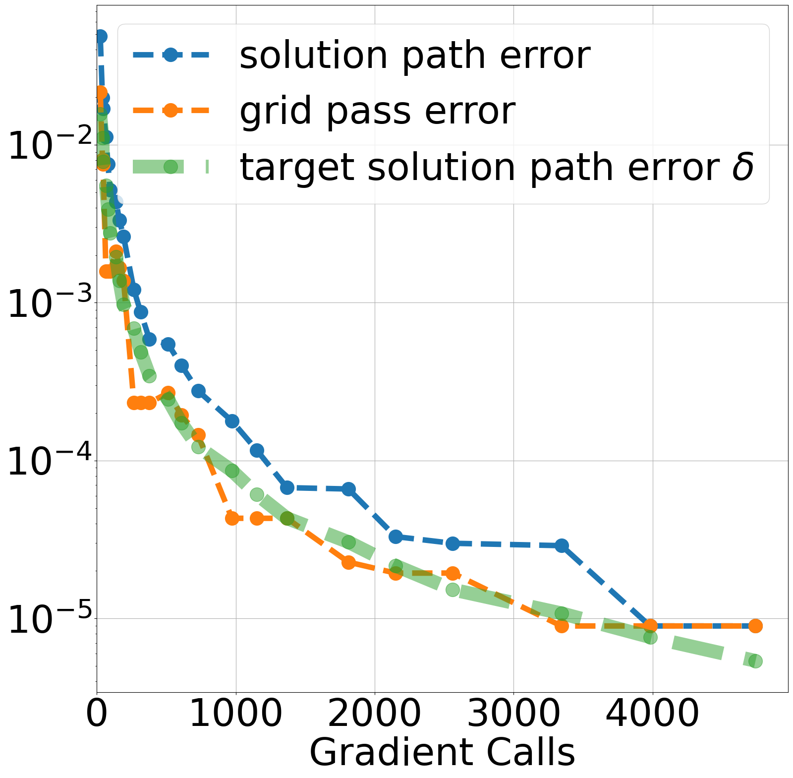
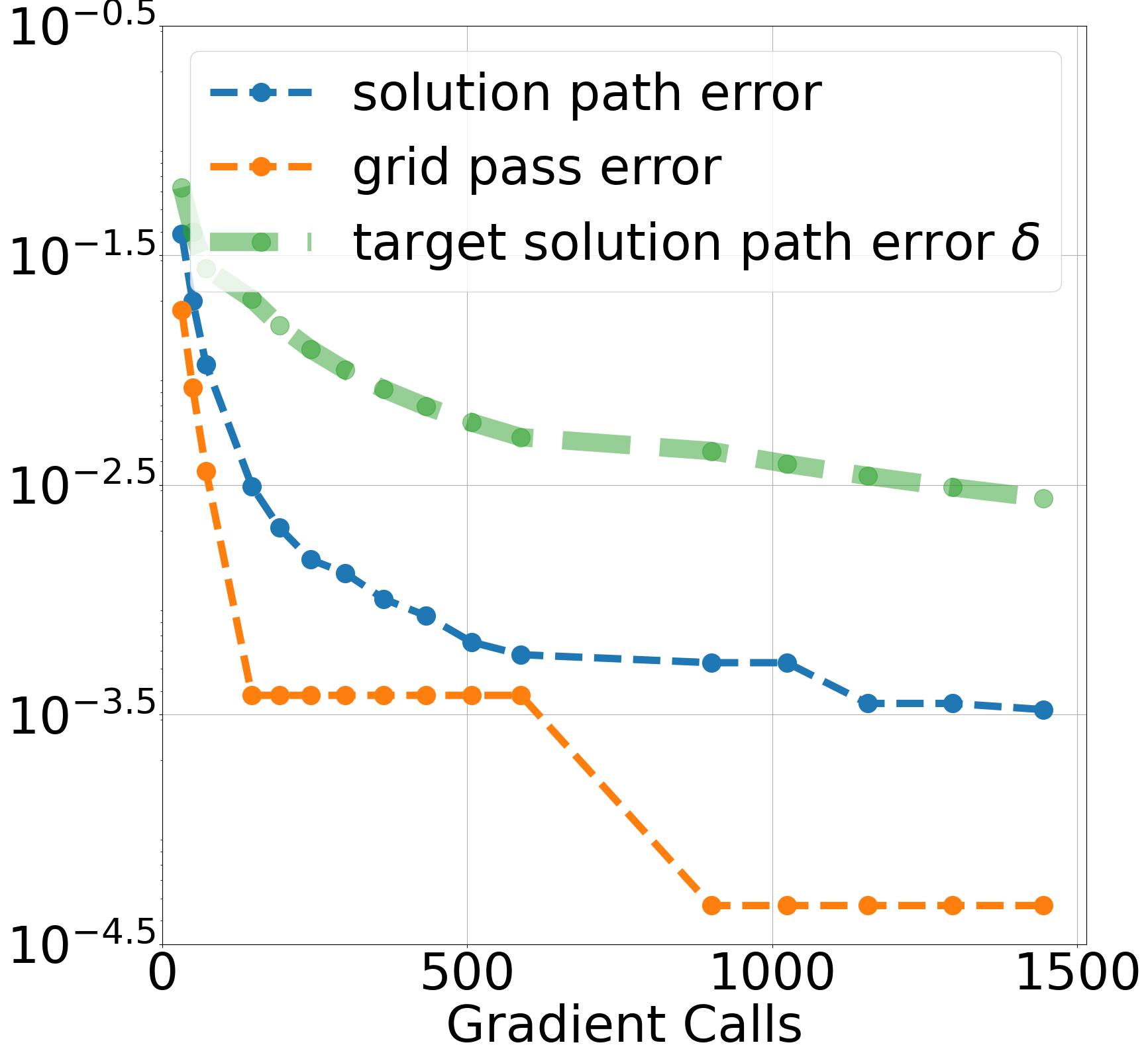
Refer to caption

(a)
Refer to caption
(b)
Figure 4: Compare: Ideal Stopping Criterion, Grid Pass Error, and Solution Path Error. (a) weighted binary classification; (b) portfolio allocation. Solution path error and grid pass error are plotted against the corresponding total number of gradient calls incurred in practice. Target solution path error δ𝛿\delta is plotted against c1log(c2/δ)/δsubscript𝑐1subscript𝑐2𝛿𝛿c_{1}\log(c_{2}/\delta)/\sqrt{\delta}, which also equals the total number of gradient calls incurred in practice. Each discrete point in the line plots above corresponds to a discretization grid point δG(δ)𝛿𝐺𝛿\delta\in G(\delta); thus smaller δ𝛿\delta is associated with more gradient calls.

Appendix C Additional Figures

Refer to caption

Refer to caption
Figure 5: 𝜽(λ)superscript𝜽𝜆\boldsymbol{\theta}^{*}(\lambda) for Portfolio Allocation from Section 6.2. The true solution paths are very smooth in each dimension, suggesting that this problem is highly interpolable by a polynomial basis.
Refer to caption
Figure 6: LSP and ALSP for Portfolio Allocation. Compares methods using the first p=4,9,16𝑝4916p=4,9,16 bivariate-Legendre polynomials. Differs from Figure 3 as the y𝑦y-axis records the number of function evaluations during line-search of BFGS instead of gradient calls.