Bin-Conditional Conformal Prediction of Fatalities from Armed Conflict

Abstract

Forecasting of armed conflicts is an important area of research that has the potential to save lives and prevent suffering. However, most existing forecasting models provide only point predictions without any individual-level uncertainty estimates. In this paper, we introduce a novel extension to conformal prediction algorithm which we call bin-conditional conformal prediction. This method allows users to obtain individual-level prediction intervals for any arbitrary prediction model while maintaining a specific level of coverage across user-defined ranges of values. We apply the bin-conditional conformal prediction algorithm to forecast fatalities from armed conflict. Our results demonstrate that the method provides well-calibrated uncertainty estimates for the predicted number of fatalities. Compared to standard conformal prediction, the bin-conditional method outperforms offers improved calibration of coverage rates across different values of the outcome, but at the cost of wider prediction intervals.

Keywords Conformal prediction  $\cdot$ Conflict forecasting  $\cdot$ Prediction intervals  $\cdot$ skewed distributions

1 Introduction

In recent years, forecasting of armed conflict has been propelled to the mainstream of conflict research. Numerous ambitious projects now aim to predict a wide range of political and conflict related outcomes [9, 7, 14, 2, 13, 20, 23, e.g.]. Although the field of conflict forecasting has advanced significantly in the last several years, most of the predicted outcomes are still expressed as point predictions without individual-level uncertainty metrics attached. Instead, aggregate error rates are usually reported to evaluate the overall performance of the models.

We argue that relying solely on point predictions at the individual forecasting level, while assessing the model performance only at the aggregate level, is problematic for several reasons. First, while point predictions may be reasonably accurate and give an important signal to stakeholders, they will most often be incorrect. Without accompanying uncertainty estimates around the point estimates, the utility of these point predictions to stakeholders is thus greatly reduced. This is especially concerning in fields where the outcomes to be forecasted are rare events with potentially large impacts, such as when forecasting the severity of armed conflicts. Point predictions in these cases tend to be pushed towards zero due to the rarity of the events. This in turn may risk underestimating the likelihood of high impact and high fatality events, unless the uncertainty of the individual predictions are taken into account [8].

Second, point predictions without uncertainty measures are inadequate for effective communication. Policymakers and other stakeholders are often less interested in the point prediction itself than with the risk associated with a given phenomenon. For instance, the best point prediction for a non-violent but stable country in a given month is typically 0 fatalities, but the probabilities of more than 1,000 deaths or even 100,000 may be alarmingly high. Performing a simple prediction of the probability of exceeding a fatality threshold [7, as in ] addresses this, but does not make good use of available count data. In order to adequately assess risk, we need appropriate and well-calibrated prediction intervals around point prediction values.

Third, while aggregate performance metrics such as mean squared error, accuracy, areas under the receiver operator characteristics and precision-recall curves, or continuous rank probability scores may provide useful information about the overall performance of the model, they do not offer insight into the uncertainty associated with any given individual prediction.

In this paper, we address these problems associated with point predictions in conflict forecasting through the use of conformal prediction. Conformal prediction allows for the estimation of individual-level prediction intervals from any arbitrary prediction model, which under certain conditions guarantees a user-specified level of coverage. However, standard conformal prediction algorithms only maintain marginal coverage and do not guarantee uniform levels of coverage across different subsets of the data.

To address this issue, we introduce a new method called bin-conditional conformal prediction (BCCP). This method ensures that prediction intervals have the correct coverage rate not only in the aggregate, but also over different, user-defined, subsets (bins) of the data. We demonstrate the effectiveness of this method first on simulated data and then on real data from one of the Violence Early Warning System (ViEWS) fatality forecasting models. The results show that the bin-conditional conformal prediction intervals achieve appropriate coverage rates both in aggregate and over different subsets of the data. In contrast, the standard conformal prediction intervals achieve appropriate coverage only in aggregate, but exhibit over- and under-coverage across different subsets of the data.

We conclude by discussing the implications of these findings for the field of conflict- and political forecasting, and the potential future developments of the method. Our bin-conditional conformal prediction algorithm for continuous data is available in the R-package pintervals on CRAN.

2 Conformal Prediction

Conformal prediction is a general purpose, model-agnostic, method that, given any point prediction, $\hat{y}$, any desired error rate, $\alpha\in[0,1]$, and any measure of dissimilarity (non-conformity), can be used to create a prediction interval around $\hat{y}$ that with probability of $1-\alpha$ contains the true value/label $y$. Under the condition that the dissimilarity scores are exchangeable (not necessarily independent and identically distributed), conformal prediction sets are mathematically guaranteed to be calibrated to their user-specified level of coverage in repeated sampling [21, 18].

Conformal prediction is especially attractive because it is model-agnostic, i.e. that it can be applied to any prediction algorithm that outputs a point prediction, regardless of whether the point prediction is regression or classification and whether or not the prediction algorithm outputs any uncertainty measures. This means that conformal prediction can be applied on top of machine learning algorithms such as random forests, boosted tree models, and support vector machines without requiring any further adaptation [5, 18]. Since its introduction in 1999 [17, 22], conformal prediction has been applied to a wide range of prediction problems and algorithms [5, for a review, see].

2.1 Assumptions of Conformal Prediction

Conformal prediction applies to settings for which we wish to obtain a $1-\alpha$ level prediction interval for some label $y_{n+1}$, associated with feature $x_{n+1}$, based on a set of $n$ example feature-label pairs, $(x_{1},y_{1}),\dots,(x_{n},y_{n})$. The conformal prediction set at level $1-\alpha\in[0,1]$ associated with $x_{n+1}$ will include the true label $y_{n+1}$ with probability at least $1-\alpha$, provided the non-conformity scores for $(x_{1},y_{1}),\dots,(x_{n},y_{n}),(x_{n+1},y_{n+1})$ are exchangeable in the sense of Definition 1.

Definition 1 (Exchangeability)

A sequence $Y_{1},Y_{2},\dots$ with probability measure $P$ is said to be exchangeable if for every integer $n>0$, every permutation $\sigma$ on $\{1,\dots,n\}$, and every $P$ measurable set $E$, $P\big{\{}(Y_{1},\dots,Y_{n})\in E\big{\}}=P\big{\{}(Y_{\sigma(1)},\dots,Y_{\sigma(n)})\in E\big{\}}.$

The non-conformity score for $(x_{i},y_{i})$ is a measure of dissimilarity between $(x_{i},y_{i})$ and $(x_{1},y_{1}),\dots,(x_{i-1},y_{i-1})$, $(x_{i+1},y_{i+1}),\dots,(x_{n+1},y_{n+1})$. A non-conformity score can be constructed from any real-valued function that is invariant to the order of points $(x_{1},y_{1}),\dots,(x_{i-1},y_{i-1}),(x_{i+1},y_{i+1}),\dots,(x_{n+1},y_{n+1})$, but is generally taken as any real-valued error function for a predictive algorithm such as: the absolute or squared error between the predicted and true values for regression problems, distance to nearest neighbor in nearest neighbor classification, or one minus the soft-max activation function components of a neural network [4, e.g.,], etc.

To obtain the $1-\alpha$ prediction set for $y_{n+1}$ we calculate the non-conformity score for our test case using $x_{n+1}$ and a range of hypothetical values which $y_{n+1}$ may have. If the support of the prediction values is finite (as in classification), then all possible labels are considered as the hypothetical values, while if the support is infinite (as in real-valued regression), then a grid of reasonable hypothetical values based on $x_{n+1}$ is iterated over. For each hypothetical $y_{n+1}$ value a p-value is computed as the proportion of non-conformity scores in the training data that are larger than the non-conformity score for the hypothetical $y_{n+1}$ value. The $1-\alpha$ prediction set is constructed by including in it all hypothetical values of $y_{n+1}$ corresponding to a p-value larger than $\alpha$ [18, 19].

2.2 Transductive and Inductive Conformal Prediction

The non-conformity scores can be obtained either transductively and inductively. The main difference between these approaches is that transductive conformal prediction requires the prediction algorithm to be re-trained for every new test case, while inductive conformal prediction splits the training data into a training set and a calibration set. In the inductive case, the the prediction algorithm is then trained on the training set and out-of-sample predictions and associated non-conformity scores are calculated using the calibration partition. These non-conformity scores are then used when creating the prediction set for the new test case [19, 15]. For computationally demanding machine learning algorithms, the inductive approach is more practical as it avoids re-training the data for each test case, although it incurs a loss of power due to the splitting of the data [19].

2.3 Local Coverage of Conformal Prediction

Conformal prediction is mathematically guaranteed to produce prediction sets having finite-sample control over type I error rates, for any user-specified level of significance. However, while this property holds in aggregate over repeated sampling, this property does not necessarily hold conditionally on subsets of labels if $y$ is categorical, or conditionally on regions of values, if $y$ is real-valued [6, see for instance]. In particular, when the outcome $y$ suffers from severe class imbalance or is heavily skewed the standard conformal prediction algorithm will tend to over-cover denser regions and under-cover sparse regions of $y$.

One proposed method for achieving appropriate coverage on subsets of the label space is to use label-conditional conformal prediction, where the prediction set is calculated using only the non-conformity scores of $y$’s associated with the same label as the hypothetical label of the test case. This approach guarantees that the prediction set will have the correct coverage both in the aggregate and for each label of $y$ [19].

This approach of label-conditional conformal prediction can easily be extended to real-valued $y$’s, where the labels can represent different regions in time or space, for instance. In this case, the resulting prediction sets are calibrated to the local distribution of the calibration data in each label-class and will therefore, under the assumption of exchangeability, have the correct coverage in each label-class. This has been shown to work well in practice when predicting housing prices for different districts in a city [11].

2.4 Bin-conditional Conformal Prediction

Not all types of data have a natural clustering structure that can be used to condition the label-conditional conformal prediction algorithm. However, they may still suffer from non-uniform coverage across the range of the outcome space of $y$ [6]. This is especially a concern in cases where the outcome $y$ is real-valued and the distribution of $y$ is skewed or multimodal, which is not uncommon in social science applications. Using a standard continuous conformal prediction approach in these cases will generate predictions sets that have the correct coverage in the aggregate, but which may not have the correct coverage across all values in the outcome space.

A field with notoriously skewed and multimodal outcomes is the prediction of fatalities from armed conflict, where the number of fatalities is often zero but can also be very high in some cases [16, 7, see for instance]. In this case, the prediction intervals may have too high coverage in the lower range of $y$ and too low coverage in the upper range of $y$. Additionally, the most salient predictions are often those that are in the upper range of $y$, and it is therefore important that the prediction intervals have the correct coverage in this range.

To solve the problem of non-uniform coverage across the range of $y$ in real-valued outcomes, we propose to extend the label-conditional conformal prediction approach to a bin-conditional conformal prediction approach (BCCP), where the outcome space is partitioned into user-specified ranges (bins) on which the user wishes to obtain correct coverage. The bin-conditional conformal prediction approach is thus a hybrid of the label-conditional, or Mondrian, conformal prediction approach, and the standard conformal prediction approach for real-valued outcomes. This method is compatible with both inductive and transductive routines, though we focus on the inductive version here.

We specify the bin-conditional conformal prediction algorithm for the inductive routine as follows:

1. Partition the data into a training set and a calibration set.

2. Train the prediction algorithm on the training set.

3. Calculate the non-conformity score for each datum in the calibration set

4. Partition the non-conformity scores into user-specified bins based on the true $y$’s in the calibration set.

5. Set a user-specified coverage level $\alpha$ which to obtain

6. For each test case, run a standard conformal prediction algorithm conditional on each bin separately , over a grid of hypothetical $y$ values associated with each bin.

7. Calculate prediction interval for each bin by keeping the hypothetical $y$ values which produce non-conformity scores below the $1-\alpha$ quantile of the non-conformity scores of the $y$’s in the bin-conditional calibration set.

8. Combine the prediction intervals from each bin to obtain the final prediction interval(s).

This algorithm guarantees prediction intervals with correct coverage in each user-specified bin of $y$, assuming exchangeability of the data within each bin.

Two important questions arise when using the bin-conditional conformal prediction approach. The first is how to partition the $y$’s into bins. The second is how to combine the prediction intervals from each bin to obtain the final prediction interval.

2.4.1 Selecting the bins

In the bin-conditional conformal prediction approach, the choice of bins depends on what ranges of the outcome space the user is interested in obtaining correct coverage for. However, there are also some practical considerations that should be taken into account when selecting the bins. The first is that the bins should be large enough to contain a sufficient number of data points to obtain a reliable estimate of the non-conformity scores. An absolute minimum of data points are such that the $1-\alpha$ quantile of the non-conformity scores can be calculated in each bin with some precision. The second is that the bins should be small enough to capture the local distribution of $y$ in each bin, i.e. ensure that the data within the bin are, in fact, exchangeable. If the bins are too large, the prediction regions in the individual bins may suffer from the same non-uniform coverage as in the standard conformal prediction approach.

Finally, increasing the number of bins lowers the number of data points in each bin and may thus widen the intervals associated with each bin due to a loss of statistical efficiency. The choice of bins is therefore a trade-off between the width of the prediction regions and the uniformity of the coverage of the prediction regions in each bin.

2.4.2 Combining bins

A potential drawback of the bin-conditional conformal prediction approach is that the final prediction interval is not necessarily contiguous. Instead, this interval may be a union of disjoint prediction intervals. This is not necessarily a problem, but it may be less intuitive for the user or the decision-maker. In the case where the prediction intervals are disjoint, an alternative is to contiguize the intervals by using the lower and upper endpoints of the intervals across all bins. This approach guarantees that the prediction regions have at least the correct coverage in each bin but may have higher coverage than specified by $\alpha$ in some regions of the outcome space and in the aggregate.

3 Simulation study

To evaluate the performance of the bin-conditional conformal prediction algorithm, we conduct a simulation study to compare the coverage and width of the prediction intervals obtained from the bin-conditional conformal prediction algorithm to those obtained from the standard conformal prediction algorithm across different values of $y$ in the test set.

We use a simple simulation setup with two predictor features $x_{1}$ and $x_{2}$ generated as independent random uniform variables between 0 and 1, and a prediction target $y$ which is generated as a log-normal distribution with parameters $\mu=x_{1}+x_{2}$ and $\sigma=0.5$ on the log-scale. The simulated distributions are heavily right-skewed with a large proportion of near-zero values.

We generate 10,000 instances of our variables and partition these into three sets: a training set with 5,000 instances, a calibration set with 2,500 instances, and a test set with 2,500 instances. We then train a simple linear regression model on each training set using the natural logarithm of $y$ as the target variable and $x_{1}$ and $x_{2}$ as the predictor variables. Predictions are made on the original $y$-scale by exponentiating the model’s predictions.

Next, we compute the non-conformity scores on the calibration set, using the absolute prediction error as the non-conformity measure. We partition the calibration data into four bins based on the empirical 25th, 50th, and 75th percentiles of the $y$ values. To highlight the importance of the choice of bins we also consider two additional scenarios with 2 and 6 bins, again based on the empirical percentiles of the $y$ values in the calibration sets.

We then apply the bin-conditional conformal prediction algorithm to the test set using both the contiguous (BCCPc) and disjoint (BCCPd) interval approaches for $\alpha=0.1$, giving an expected coverage rate of 90%. We compare the coverage and width of the prediction intervals produced by this method to those from the standard conformal prediction (SCP) algorithm. We make this comparison both in aggregate and across ranges of $y$-values. This simulation process is repeated 1,000 times to ensure robust results.

3.1 Simulation results

The mean aggregate and bin-conditional coverage of the simulation study are shown in Table 1 below. The table displays both the aggregate coverage as well as the coverage in each of the four quartiles of $y$ for the SCP, BCCPc, and BCCPd algorithms. The results show that while the standard conformal prediction algorithm achieves correct coverage in aggregate, it fails to obtain the correct coverage across different ranges of $y$. In contrast, the bin-conditional conformal prediction algorithms achieve at least the correct coverage in aggregate as well as within each bin it is conditional on.

The results of the BCCP algorithms with two bins are especially illustrative as they show that the coverage in both the first two and last two quartiles are at least correct in aggregate, but not within the individual quartiles. The BCCP algorithms with four and six bins, on the other hand, show that the coverage is at least at the nominal level for all quartiles as well as in aggregate. As expected, bin-conditional conformal prediction with contiguized intervals (BCCPc) slightly over-covers some of the quartiles of $y$, except when using only two bins when the results are identical for the disjoint and contiguous intervals. The disjoint intervals (BCCPd) on the other hand, achieve coverage rates only marginally different from the nominal 90% in all bins they are conditional on.

Table 1: Coverage of the different conformal prediction algorithms in aggregate and across empirical quartiles (Q1-Q4) of $y$ in the simulation study. $\alpha=0.1$ and expected coverage is 0.90.

Method	Bins	Aggregate	Q1 of $y$	Q2 of $y$	Q3 of $y$	Q4 of $y$
SCP		0.899	0.99	0.98	0.99	0.64
BCCPc	2	0.899	0.89	0.91	1.00	0.80
BCCPd	2	0.899	0.89	0.91	1.00	0.80
BCCPc	4	0.912	0.90	0.90	0.95	0.90
BCCPd	4	0.898	0.90	0.90	0.90	0.90
BCCPc	6	0.919	0.90	0.90	0.95	0.93
BCCPd	6	0.898	0.90	0.90	0.92	0.88

The effect of bin selection on coverage can also be seen in Figure 1 below which shows the coverage rates across different values of the prediction target. The figure illustrates that the standard conformal prediction algorithm severely over-covers values of $y$ near zero, where most of the data are located, and under-covers on the right tail of $y$. The bin-conditional conformal prediction algorithms, on the other hand, maintain the correct aggregate coverage in each of the bins they are conditional on, although not uniformly within these bins. Comparing the BCCP algorithm with 2 and 6 bins, it is clear that the coverage is more uniform across the range of $y$ when using more bins. However, even in the case of 6 bins, the coverage drops below the nominal level of 90% for the highest values of $y$.

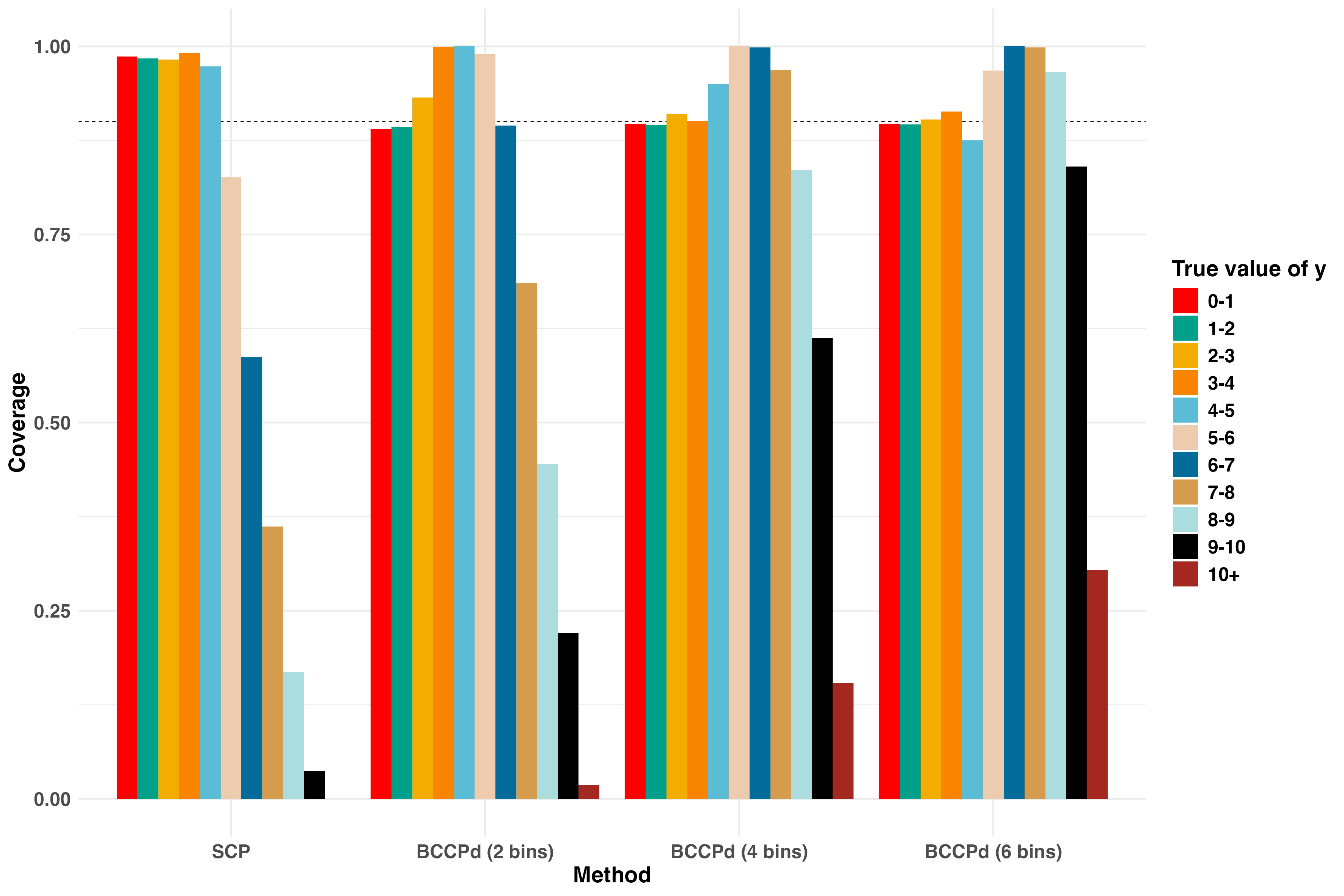
Figure 1: Coverage across different values of $y$. Only the non-contiguous version of the bin-conditional conformal prediction algorithm is shown.

The trade-off between coverage and width is illustrated in Figure 2 which shows the smoothed mean width of the prediction intervals across the range of $y$ for the different conformal prediction methods. The figure shows that the standard conformal prediction algorithm produces the narrowest intervals, and that increasing the number of bins in the bin-conditional conformal prediction method also increases the average width of the intervals. This demonstrates the tradeoff between maintaining appropriate coverage and the width of the intervals.

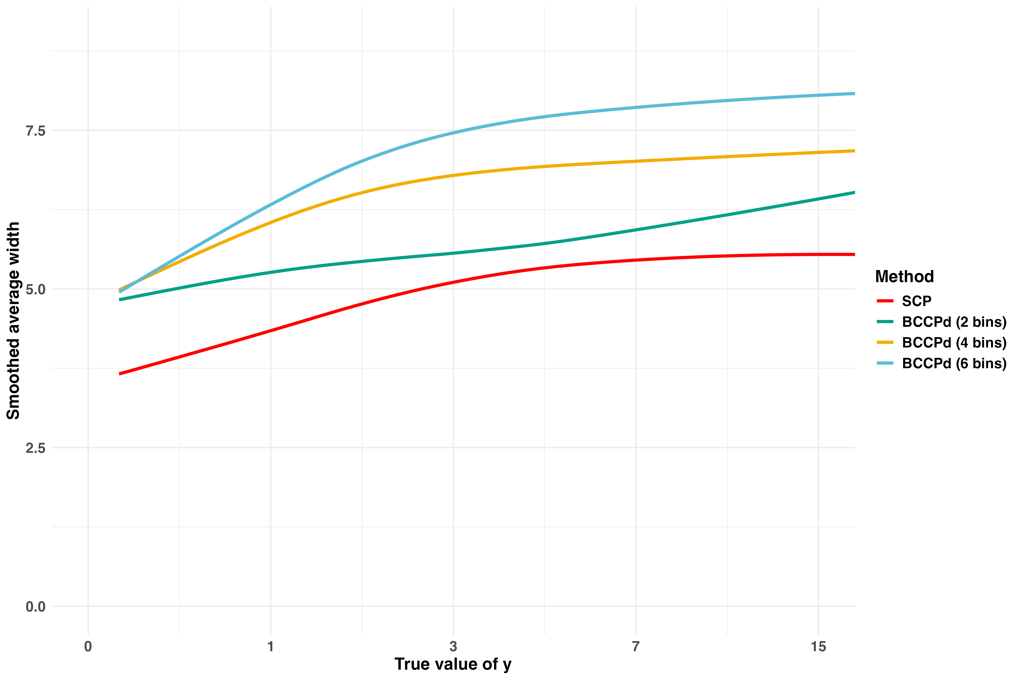
Figure 2: Mean interval width across different values of $y$. Only the non-contiguous version of the bin-conditional conformal prediction algorithm is shown. $\alpha=0.1$ and expected coverage is 0.90.

4 Bin-conditional conformal prediction of fatalities from armed conflict

To test the practical application of the bin-conditional conformal prediction algorithm and compare it to the standard conformal prediction algorithm, we apply both methods to a prediction model for fatalities from armed conflict. Specifically, we apply the algorithms to one of the constituent models from the Violence Early Warning System (VIEWS) fatalities forecasting project [10]. The model we use is the broad topics constituent model, inspired by [14], which consists of a set of 64 predictor features including a number derived from 15 different topics covered in new articles. The prediction target is the number of fatalities from armed conflict in which at least one of the actors is a state [3], for each country month between the years 2000 and 2022.

The prediction target in this application exhibits characteristics that may be challenging from a prediction standpoint. In particular, the prediction target is severely zero-inflated and highly right-skewed with approximately 86.7% being zeroes and the top 1% of the observations accounting for nearly 75% of the fatalities.

We obtain the predictions using a standard random forest regressor. In line with VIEWS standards, we make predictions for the number of fatalities on the log1p scale i.e. log(fatalities+1) [10]. To test whether the prediction intervals we obtain have a correct level of coverage, we run a set of 1,000 simulations where we randomly partition our data into training (70%), calibration (20%), and test (10%).

In each simulation, we train the random forest model using the randomly assigned training data, we then calculate the non-conformity scores by making out-of-sample prediction on the calibration data, and finally we calculate the prediction intervals on the test data and compute the coverage of the prediction intervals. We run both a standard conformal prediction algorithm and the disjoint bin-conditional conformal prediction algorithm using 2, 4, and 7 bins. In the two-bin version, we split the calibration data into bins based on true zeroes versus non-zeroes. In the seven-bin versions we keep one bin for zeroes and then split the non-zeroes into six bins based on a logarithmically increasing number of fatalities in each bin such that the bins are defined in the following way; bin 1: 0 fatalities, bin 2: 1–2 fatalities, bin 3: 3–7 fatalities, bin 4: 8–20 fatalities, bin 5: 21–54 fatalities, bin 6: 55–148 fatalities, and bin 7: 149+ fatalities. In the four-bin version, we use the same binning structure as the seven-bin version but combine bins 2–3, 4–5, and 6–7. The binning structure we have chosen is essentially arbitrary, but does result in bins with approximately similar number of observations outside the bin for zeroes. We do not claim that this is the optimal binning structure for these data but rather a first attempt to explore the potential of the bin-conditional conformal prediction algorithm on this type of data. Across all simulations we use $\alpha=0.1$ giving an expected coverage of 90% for the prediction intervals.

A further issue with this prediction problem is that since the prediction target is the log1p transformed counts of fatalities, the prediction target is not strictly continuous but rather quasi-continuous, where the true values are restricted to the log1p transformation of all positive integers. This also poses a challenge to the continuous conformal prediction algorithm since it limits the valid values of the prediction interval. To deal with this problem, we make our predictions and predictions interval on the original fatality scale by reversing the log1p transformation for the predictions and the prediction intervals. To ensure that the prediction intervals correspond to this data structure, we round the lower and upper bounds of the prediction intervals to the nearest integer.

4.1 Results

We begin by comparing the coverage of the algorithms in aggregate as well as across true zeroes and non-zeroes. These results can be seen in Table 2 below. These results exhibit the same pattern as in the simulation study, i.e. that while the standard continuous conformal prediction algorithm produces an aggregate coverage level close to the nominal level, it both severely over-covers the zeroes and under-covers the non-zeroes. The bin-conditional conformal prediction algorithms, on the other hand, manages to produce an appropriate level of coverage among both zeroes and non-zeroes.

Table 2: Coverage of prediction intervals for the standard conformal prediction algorithm and the bin-conditional conformal prediction algorithm with 2, 4, and 7 bins. $\alpha=0.1$ and expected coverage is 0.90.

Method	Bins	Aggregate	Zeroes	Non-zeroes
SCP		0.919	0.98	0.52
BCCPd	2	0.9	0.9	0.903
BCCPd	4	0.9	0.9	0.905
BCCPd	7	0.9	0.9	0.903

Further dividing the results, into the value ranges corresponding to the seven bins used for the bin-conditional conformal prediction algorithm, we again see that the coverage remains appropriate for the number of bins used. These results are shown in Figure 3 below. We also observe that while the alternative binning structures produce intervals with aggregate appropriate coverage within the bins on which they are conditional, they obtain uniform coverage across all values of $y$ within these bins. This further highlights the flexibility of the bin-conditional conformal prediction algorithm and the importance of setting the number of bins so that the coverage is appropriate across the most important ranges of the prediction target.

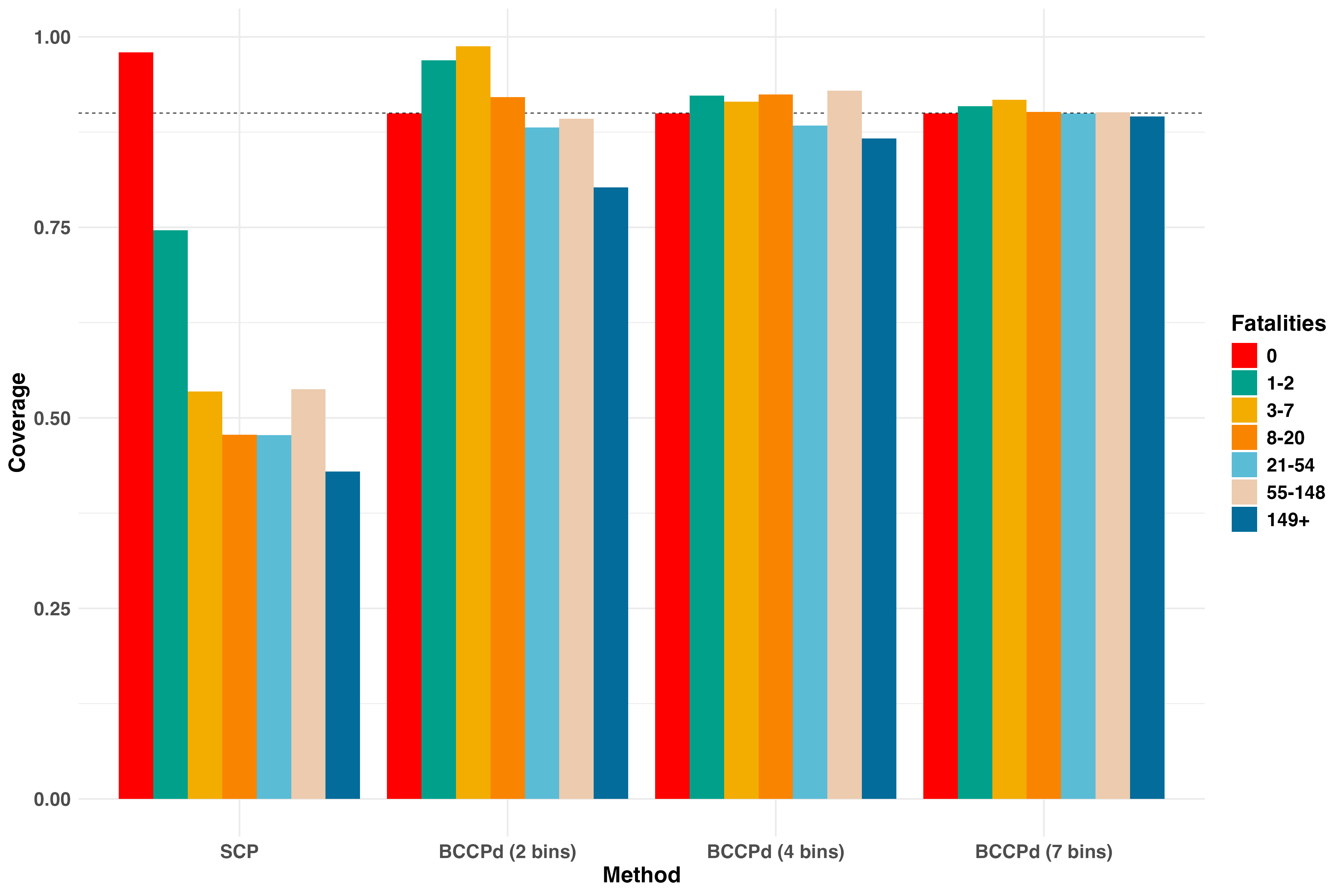
Figure 3: Coverage of prediction intervals for the different conformal prediction methods across the seven bins in the data. Only the disjoint versions of the BCCP algorithm are shown.

Increasing the number of bins for the BCCP algorithms does, however, come at the cost of wider intervals. The mean widths of the intervals are shown in Figure 4 below. Here we again see that the bin-conditional conformal prediction algorithm produces intervals which on average are wider than the standard conformal prediction algorithm. We can also see that the average width again increases with the number of bins used in the bin-conditional conformal prediction algorithm. In practice, this is a tradeoff where the user needs to weigh the uniformity of the coverage rate with the width of the resulting intervals.

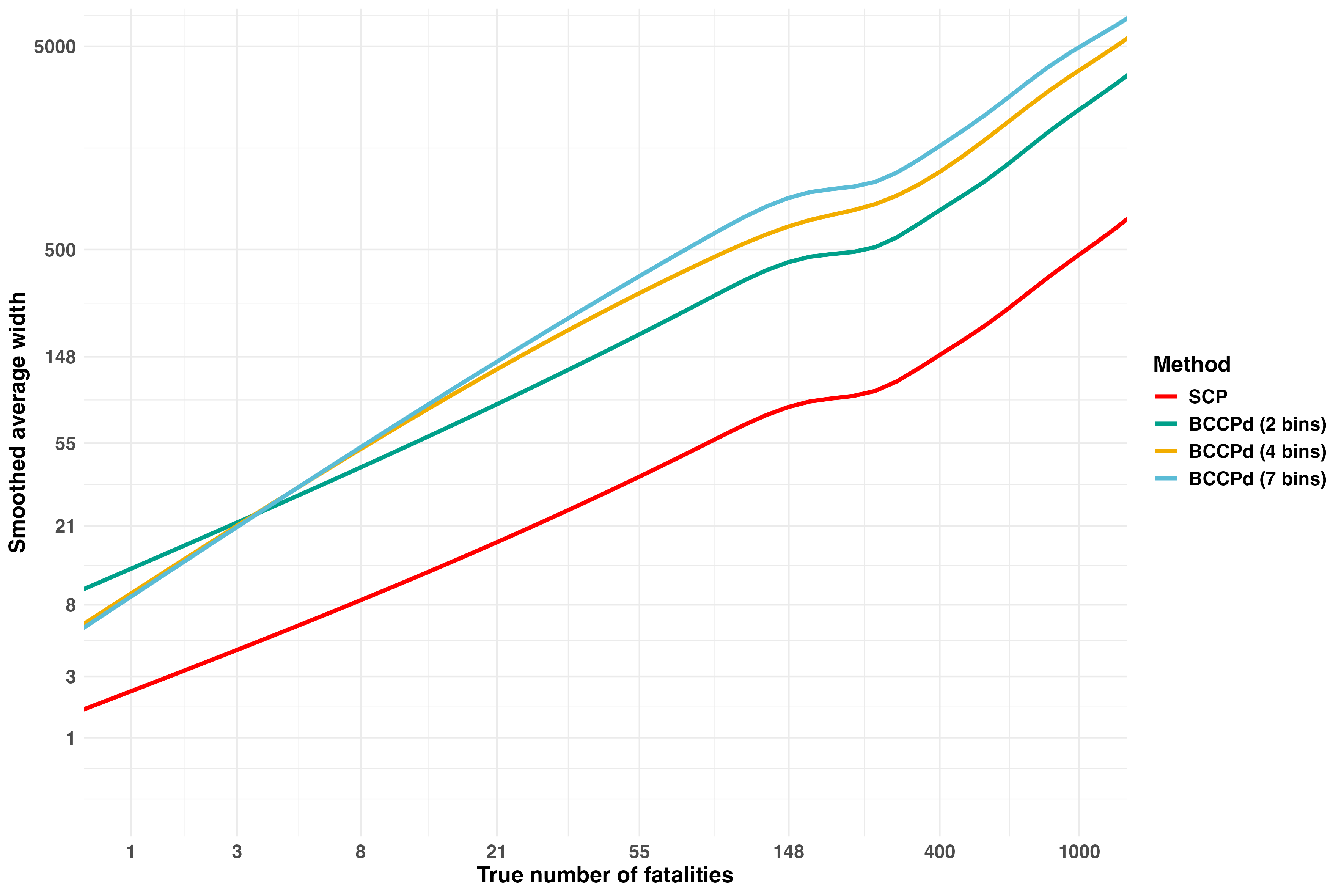
Figure 4: Mean width of prediction intervals for the different conformal prediction methods across different number of fatalities.

5 Discussion

In this paper, we have introduced a new conformal prediction algorithm that maintains an appropriate level of coverage across different ranges of the prediction target. When the prediction target has a heavily right-skewed and/or zero-inflated distribution, standard conformal prediction approaches fail in producing correct coverage. We demonstrated that our bin-conditional conformal prediction method achieves correct coverage within user-defined bins of values, although at the cost of wider prediction intervals. The method performed well in both a simulation study and in a real-world application predicting the number of fatalities from armed conflict.

Furthermore, this paper has highlighted the need for developing methods that allows researchers to produce forecasts which not only give point predictions, but also accurate and interpretable prediction intervals. The bin-conditional conformal prediction algorithm extends the applicability of conformal prediction algorithms to a wider range of prediction problems, as it allows the user to define the most important ranges of the prediction target and ensures that the prediction intervals are calibrated within these ranges. This may be particularly important in fields where the end users of the predictions are not experts in statistics and machine learning but rather stakeholders or policymakers who may need to make decisions based on the predictions.

The algorithms within the Conformal Prediction framework assume that the predictions from the models are exchangeable, meaning that their order does not matter. In the context of conflict prediction, this assumption may not hold as the data generating process may change over time. Despite this potential limitation, the strong performance of the bin-conditional conformal prediction algorithm in the real-world application suggests that the method may be robust to some violations of this assumption. Additionally, the general approach presented in this paper may also easily be combined with other methods developed for conformal prediction in applications which do not necessarily fulfill the exchangeability assumption [1, 12, 11, see for instance].

Selecting the number of bins to use in the bin-conditional conformal prediction algorithm is a crucial step in the application of the method. In this paper, we have argued that the number of bins should be set so that the coverage is appropriate across the most important ranges of the prediction target. However, the optimal number of bins may vary depending on the application and the prediction target. Future research should investigate methods for selecting the number of bins in the bin-conditional conformal prediction algorithm in a data-driven manner, for instance by using cross-validation or other model selection techniques.

We have made the bin-conditional conformal prediction algorithm available in the pintervals package for R on CRAN.

References

- [1] Rina Foygel Barber, Emmanuel J Candes, Aaditya Ramdas and Ryan J Tibshirani “Conformal prediction beyond exchangeability” In The Annals of Statistics 51.2 Institute of Mathematical Statistics, 2023, pp. 816–845
- [2] Curtis Bell “Coup d’état and democracy” In Comparative Political Studies 49.9 Sage Publications Sage CA: Los Angeles, CA, 2016, pp. 1167–1200
- [3] Shawn Davies, Therése Pettersson and Magnus Öberg “Organized violence 1989–2022, and the return of conflict between states” In Journal of Peace Research SAGE Publications Sage UK: London, England, 2023, pp. 00223433231185169
- [4] Neil Dey et al. “Conformal Prediction for Text Infilling and Part-of-Speech Prediction” In The New England Journal of Statistics in Data Science 1 New England Statistical Society, 2023, pp. 69–83
- [5] Matteo Fontana, Gianluca Zeni and Simone Vantini “Conformal prediction: a unified review of theory and new challenges” In Bernoulli 29.1 Bernoulli Society for Mathematical StatisticsProbability, 2023, pp. 1–23
- [6] Leying Guan “Localized conformal prediction: A generalized inference framework for conformal prediction” In Biometrika 110.1 Oxford University Press, 2023, pp. 33–50
- [7] Håvard Hegre et al. “ViEWS2020: revising and evaluating the ViEWS political violence early-warning system” In Journal of peace research 58.3 SAGE Publications Sage UK: London, England, 2021, pp. 599–611
- [8] Håvard Hegre et al. “The 2023/24 VIEWS Prediction Challenge: Predicting the Number of Fatalities in Armed Conflict, with Uncertainty” In arXiv preprint arXiv:2407.11045, 2024
- [9] Håvard Hegre et al. “ViEWS: A political violence early-warning system” In Journal of peace research 56.2, 2019, pp. 155–174
- [10] Håvard Hegre et al. “Forecasting Fatalities”, Uppsala: working paper, 2022 URL: https://www.diva-portal.org/smash/get/diva2:1667048/FULLTEXT01.pdf
- [11] Anders Hjort, Gudmund Horn Hermansen, Johan Pensar and Jonathan P Williams “Uncertainty quantification in automated valuation models with locally weighted conformal prediction” In arXiv preprint arXiv:2312.06531, 2023
- [12] Huiying Mao, Ryan Martin and Brian J Reich “Valid model-free spatial prediction” In Journal of the American Statistical Association 119.546 Taylor & Francis, 2024, pp. 904–914
- [13] Richard Morgan, Andreas Beger and Adam Glynn “Varieties of forecasts: Predicting adverse regime transitions” In V-Dem Working Paper 89, 2019
- [14] Hannes Mueller and Christopher Rauh “Reading between the lines: Prediction of political violence using newspaper text” In American Political Science Review 112.2 Cambridge University Press, 2018, pp. 358–375
- [15] Harris Papadopoulos “Inductive conformal prediction: Theory and application to neural networks” In Tools in artificial intelligence Citeseer, 2008
- [16] David Randahl and Johan Vegelius “Inference with extremes: Accounting for Extreme Values in Count Regression Models” In International Studies Quarterly, forthcoming
- [17] C Saunders, A Gammerman and V Vovk “Transduction with confidence and credibility” In Proceedings of the 16th international joint conference on Artificial intelligence-Volume 2, 1999, pp. 722–726
- [18] Glenn Shafer and Vladimir Vovk “A Tutorial on Conformal Prediction.” In Journal of Machine Learning Research 9.3, 2008
- [19] Paolo Toccaceli and Alexander Gammerman “Combination of inductive mondrian conformal predictors” In Machine Learning 108 Springer, 2019, pp. 489–510
- [20] Paola Vesco et al. “United they stand: Findings from an escalation prediction competition” In International Interactions 48.4 Taylor & Francis, 2022, pp. 860–896
- [21] Vladimir Vovk, Alexander Gammerman and Glenn Shafer “Algorithmic learning in a random world” Springer Science & Business Media, 2005
- [22] Volodya Vovk, Alexander Gammerman and Craig Saunders “Machine-Learning Applications of Algorithmic Randomness” In Proceedings of the Sixteenth International Conference on Machine Learning, 1999, pp. 444–453
- [23] Jonathan P Williams et al. “Bayesian hidden Markov models for latent variable labeling assignments in conflict research: Application to the role ceasefires play in conflict dynamics” In Annals of Applied Statistics 18.3 Institute of Mathematical Statistics, 2024, pp. 2034–2061