Reversals of toroidal magnetic field in local shearing box simulations of accretion disc with a hot corona

Abstract

Presence of a hot corona above the accretion disc can have important consequences for the evolution of magnetic fields and the Shakura-Sunyaev (SS) viscosity parameter $\alpha$ in such a strongly coupled system. In this work, we have performed three-dimensional magnetohydrodynamical (3D-MHD) shearing-box numerical simulations of accretion disc with a hot corona above the cool disc. Such a two-layer, piece-wise isothermal system is vertically stratified under linear gravity and initial conditions here include a strong azimuthal magnetic field with a ratio between the thermal and magnetic pressures being of order unity in the disc region. Instabilities in this magnetized system lead to the generation of turbulence, which, in turn, governs the further evolution of magnetic fields in a self-sustaining manner. Remarkably, the mean toroidal magnetic field undergoes a complete reversal in time by changing its sign, and it is predominantly confined within the disc. This is a rather unique class of evolution of the magnetic field which has not been reported earlier. Solutions of mean magnetic fields here are thus qualitatively different from the vertically migrating dynamo waves that are commonly seen in previous works which model a single layer of an isothermal gas. Effective $\alpha$ is found to have values between 0.01 and 0.03. We have also made a comparison between models with Smagorinsky and explicit schemes for the kinematic viscosity ($\nu$). In some cases with an explicit $\nu$ we find a burst-like temporal behavior in $\alpha$.

1 Introduction

A wide range of regimes of astrophysical MHD find their application in accretion discs around compact objects, which make these systems among the most explored in astrophysics for the past half a century (Pringle, 1981; Balbus & Hawley, 1998; Abramowicz & Fragile, 2013). The complex radiative features observed from these systems such as outbursts of dwarf novae & low mass X-ray binaries (Warner, 2003; Smak, 2000; Lewin & van der Klis, 2006; Bagnoli et al, 2015) and aperiodic variabilities of X-ray binaries (Remillard & McClintock, 2006; Lewin & van der Klis, 2006; Belloni, 2010) & AGNs (Pica, Smith et al, 1988; Giveon, Maoz et al, 1999; Ishibashi & Courvoisier, 2009; Sartori et al, 2018) indicate the existence of different limits of accretion. Temporal evolution of radiative output of the accretion systems are attributed to different phases of inner sub-Keplerian accretion flow such as Advection Dominated Accretion Flow (ADAF) (Narayan & Yi, 1994, 1995; Abramowicz et al, 1995; Fender, Belloni & Gallo, 2004; Belloni et al, 2005; Remillard & McClintock, 2006; Kylafis & Belloni, 2015), Convection Dominated Accretion Flow (CDAF) (Igumenshchev & Abramowicz, 1999), adiabatic inflow-outflow solution (ADIOS) (Blandford & Begelman, 1999), luminous hot accretion flow (LHAF) (Yuan, 2001), jet (Romero et al, 2003; Bosch-Ramon, Aharonian & Paredes, 2005; Piano et al, 2012) corona (de Gouveia Dal Pino & Lazarian, 2005; de Gouveia Dal Pino et al, 2010; Kadowaki et al, 2015) etc, fed by the outer standard cool Keplerian flow (Shakura & Sunyaev, 1973; Novikov & Thorne, 1973). Each of these phases of the accretion flow is characterised by an appropriate $\alpha$ parameter and cooling mechanisms (Yuan & Narayan, 2014) determined by mass accretion rate.

From the spectral analysis of AGNs and X-ray transients, now it is fairly understood that the accretion discs around black holes and neutron stars are hot optically thin geometrically thick flow domain surrounded by a much larger optically thick geometrically thin disc. In the transition region these two flow domain can coexist where a cool disc is embedded in a hot coronal flow (Wojaczyński et al, 2015; Inoue et al, 2019; Gutiérrez, Vieyro & Romero, 2021). Such a structure raises the possibility of interaction of cool disc and hot corona. The radiative transport of the disc will be affected by the presence of hot corona and the global mass-energy exchange of the disc-corona system is modelled separately (Meyer-Hofmeister, Liu & Qiao, 2017; Haardt & Maraschi, 1991; Meyer, Liu & Meyer-Hofmeister, 2000; Liu et al, 2015; Qiao & Liu, 2017). Moreover, the hydrodynamic and magnetic components of the viscous stress could seriously be modified in shear flow with such a strong vertical temperature jump. Therefore it is important to analyse the temporal evolution of the local shearing patch corresponding to the disc-corona system and study the exchange of matter and magnetic energy.

The disc-corona interaction is fairly universal and many phenomena associated to accretion systems can be reduced to such a topology. In the rest of the introduction we briefly identify a few such cases. Interaction between the outer disc and the radiation originating from the very inner part of the disc was suggested in the context of outburst in dwarf nova and X-ray transients (Paradijs & McClintock, 1995; Lasota, 1999). The thermo-viscous instabilities causing these outburst are modelled as influenced by this radiation exposure (van Paradijs & Mc Clintock, 1994; King & Ritter, 1998; Lasota, 2001). Later on it was shown that (RoÂzÇanÂska & Czerny, 1996; RoÂzÇanÂska, 1999; Macioøek-NiedzÂwiecki, Krolik & Zdziarski, 1997) the heating of the outer disc from top by the radiation originating from the inner part of the disc could create a hot corona above the cool disc. A transition region of sharp temperature gradient between the hot coronal layer of temperature $\sim 10^{9}$ K and the disc of temperature $\sim 10^{4}$ K is created. Such a configuration is shown to be unstable which will spontaneously create hot coronal clouds above the cool disc. The interaction between the disc and the hot coronal patches could influence the evolution of the disc properties particularly when they are magnetically coupled.

The physical mechanisms operating in accretion systems of different scales such as X-ray binaries and quasars are similar in nature. However since the sources of the matter inflow are different, the very outer part of the discs themselves may have different topologies. In the case of X-ray binaries the matter is supplied by Roche Lobe overflow and hence the outer disc is mostly concentrated about the midplane of the disc. In the case of quasars or AGN’s the matter is sourced by the hot wind from surrounding stars and hence the outer disc itself could have a relatively denser corona (Liu et al, 2015; Qiao & Liu, 2017). Hence in this context also the interaction between the disc and corona could play crucial role in the dynamical evolution of the accretion system.

Magneto Rotational Instability (MRI) (Chandrasekhar, 1960; Balbus & Hawley, 1991) and origin of turbulent viscosity in accretion disc has been discussed by numerous authors particularly with the types of initial magnetic field configurations such as an effective poloidal magnetic field (Hawley, Gammie & Balbus, 1995; Bai & Stone, 2013; Salvesen et al, 2016b), a zero net initial magnetic field or a weak toroidal field (Brandenburg et al, 1995; Miller & Stone, 2000; Davis, Stone & Pessah, 2010; Simon, Beckwith & Armitage, 2012). The measured value of $\alpha$ viscosity parameter in numerical experiments is smaller than at least by an order of magnitude of the expected value (King, Pringle & Livio, 2007). Various modifications and generalisations such as gravitational stratification, radially extended flow domain and effect of radiative transport were explored by different authors (Miller & Stone, 2000; Hirose, Krolik & Stone, 2006; Winters, Balbus & Hawley, 2003). Numerical experiments on the vertically extended disc could generate magnetically dominated corona above a gas pressure dominated disc (Salvesen et al, 2016b; Kadowaki et al, 2018) for sufficiently strong initial magnetic field. Heating due to magnetic reconnection (Liu, Mineshige & Ohsuga, 2003; Huang, Wu & Wang, 2014) in this magnetically dominated corona could create a sharp temperature gradient across “the cool disc – hot corona system”.

For all the plausible scenarios mentioned above, a vertically extended disc with temperature jump symmetrically above and below the mid-plane is a simple and faithful representation of the actual physical problem. On a global scale, the mass exchange between disc and corona, conduction from hot corona to cool disc and the Comptonization of soft photons from disc by hot corona are the main interaction processes (Meyer, Liu & Meyer-Hofmeister, 2000; Różańska & Czerny, 2000; Remillard & McClintock, 2006; Belloni & Motta, 2016). Whereas on a local scale the interesting scenarios are the growth and evolution of magnetic field topology; hydrodynamic & magneto-hydrodynamic instabilities and the effective viscous stress produced; and oscillations at the disc corona interface.

We have studied a local 3D-MHD numerical simulations using a shearing box approximation (Hawley, Gammie & Balbus, 1995) considering an initial stratified density distribution due to a linear gravity profile in the vertical direction and strong toroidal magnetic field. The disc corona system is mimicked by imposing a temperature jump symmetrically in the vertical direction. This patch of combined disc corona system is allowed to evolve for several rotation times. The paper is organised as follows: in Sect. 2 we the setup of our model, in Sect. 3 we have presented the results. We then discuss our findings and conclude in Sect. 4.

2 Model & Numerical Setup

We numerically model a local patch of an accretion disc with a hot corona above by solving fully compressible hydromagnetic equations using the publicly available Pencil Code which is a high-order, finite-difference, modular, MPI code. Basic equations being solved may be expressed as:

$$\frac{D\ln\rho}{Dt} =-\bm{\nabla}\cdot\bm{v},$$ (1)

$$\frac{D\bm{v}}{Dt} =\bm{g}+\frac{1}{\rho}\left(\bm{J}\times\bm{B}-\bm{\nabla}p+\bm{\nabla}\cdot 2\nu\rho\bm{\mathsf{S}}\right)-2\Omega_{0}\hat{z}\times\bm{v}$$ (2)

$$\rho T\frac{Ds}{Dt} =2\rho\nu\bm{\mathsf{S}}^{2}+\mu_{0}\eta\mbox{\boldmath$J$}{}^{2}-\bm{\nabla}\cdot\bm{F}_{\rm SGS}-(\gamma-1)\rho c_{p}\frac{T-T_{\rm d,c}}{\tau_{\rm c}}\,,$$ (3)

$$\frac{\partial\bm{A}}{\partial t} ={\bm{v}}\times{\bm{B}}-\eta\mu_{0}{\bm{J}},$$ (4)

where $\bm{v}$ is the velocity, $D/Dt=\partial/\partial t+\bm{v}\cdot\bm{\nabla}$ is the advective time derivative, $\bm{g}$ is the gravitational acceleration with a vertically linear profile, $\hat{z}$ is the unit vector along the vertical $z$-direction, $\mathsf{S}_{ij}={\textstyle{1\over 2}}(v_{i,j}+v_{j,i})-\text@frac{1}{3}\delta_{ij}\bm{\nabla}\cdot\bm{v}$ is the traceless rate of strain tensor, where commas denote partial differentiation, $\nu={\rm const}{}$ is the kinematic viscosity, $s$ is the specific entropy, $\rho$ is the fluid density, $p$ is the pressure, ${\bm{A}}$ is the magnetic vector potential, ${\bm{B}}=\bm{\nabla}\times{\bm{A}}$ is the magnetic field, ${\bm{J}}=\mu_{0}^{-1}\bm{\nabla}\times{\bm{B}}$ is the current density, $\eta={\rm const}{}$ is the magnetic diffusivity, $\mu_{0}$ is the vacuum permeability which is taken to be unity in our units, $\gamma=c_{\rm p}/c_{\rm v}$ is the ratio of specific heats at constant pressure and density, respectively, and $T$ is the temperature.

In some cases we have also adopted a Smagorinsky model for viscosity with $\nu=\nu_{S}$ where

$$\nu_{S}=(C_{k}\Delta)^{2}\sqrt{\bm{\mathsf{S}^{2}}}\,.$$ (5)

Here, $C_{k}$ is the Smagorinsky constant and $\Delta$ is the filtering scale which is chosen to be equal to the grid spacing; see, e.g., Haugen & Brandenburg (2006). We have used $C_{k}=0.35$ in this work.

The last term in Eq. (3) is a relaxation term which guarantees that the temperatures in the two subdomains, disc and corona, remain, on average, constant and equal to $T_{\rm d}$ (disc) and $T_{\rm c}$ (corona), respectively. In the present work, we applied the relaxation term only in the corona to maintain its temperature. This is preferable as it allows the flow to evolve more freely in the disk. In one of the simulations, A1s$\chi$, we have used a subgrid-scale (SGS) diffusivity ($\chi_{\rm SGS}$) which acts on the fluctuations of the entropy about its horizontal average (Käpylä, 2021). The SGS flux is given by

$$\bm{F}_{\rm SGS}=-\rho T\chi_{\rm SGS}\bm{\nabla}s^{\prime}\;,\quad s^{\prime}=s-\langle s\rangle_{xy}$$ (6)

The angular velocity of the accretion disc at some arbitrary radius $R=R_{0}$ is denoted by $\Omega_{0}$. In rotating reference frame of the local Cartesian patch of the disc at $R_{0}$, the velocity field is in the toroidal $y$-direction with a linear shear profile:

$$\bm{V}=-q\Omega_{0}x\,\hat{y}$$ (7)

where $q=3/2$ for a Keplerian disc, and $\hat{y}$ is the unit vector along toroidal direction. The total velocity field is $\bm{v}=\bm{V}+\bm{u}$, where $\bm{u}$ is the velocity deviation.

We assume an ideal fluid with an equation of state determining its pressure by $p=(c_{\rm p}-c_{\rm v})\rho T=\rho c_{\rm s}^{2}/\gamma$, where $c_{\rm s}$ is the adiabatic sound speed. Note that we have a piecewise isothermal setup where disc (with sound speed $c_{\rm sd}$) and a hotter corona (with sound speed $c_{\rm su}$) are maintained at two different temperatures, as shown, for example in Figure 1a. The sharp jump in temperature or density at the disc-corona interface in the beginning is characterized by

$$\delta_{0}=T_{\rm c}/T_{\rm d}=c_{\rm su}^{2}/c_{\rm sd}^{2}=\rho_{i-}/\rho_{i+}\,,$$ (8)

where $\rho_{i-}$ and $\rho_{i+}$ are the densities just below and above the interface, respectively.

Table 1: Summary of runs. All runs have $H=1$, ${\rm Sh}=-1.5$, $q\equiv-S/\Omega_{0}=1.5$, and $\delta_{0}=10$.

Run Domain Grid $\beta_{0}$ ${\rm Ma}$ ${\rm Re}$ ${\rm Rm}$ Viscosity A1s$\chi$ $6H\times 6H\times 6H$ $256\times 256\times 256$ 5.7 0.28 – 70.5 Smagorinsky A2s $6H\times 6H\times 6H$ $256\times 256\times 256$ 5.7 0.31 – 78.2 Smagorinsky A3e $6H\times 6H\times 6H$ $256\times 256\times 256$ 5.7 0.16 78 39 Explicit B1e $6H\times 6H\times 6H$ $128\times 128\times 128$ 1.5 0.40 134 134 Explicit C1s $2H\times 2H\times 8H$ $128\times 128\times 320$ 3.4 0.11 – 1111 Smagorinsky

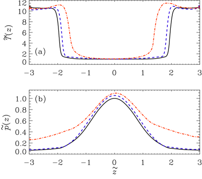
Figure 1: Profiles of (a) temperature, and (b) pressure, as functions of normalized vertical coordinate $\tilde{z}$, with $\tilde{z}=0$ being the midplane of the disc. Panels (c) and (d) display the temporal evolution of root-mean-squared values of total fluid velocity and total magnetic field, respectively. Solid (black), dashed (blue) and dash-dotted (red) curves in (a) and (b) show the profiles at three epochs in time that are marked by corresponding vertical lines in panel (d). These are shown from the run A1s$\chi$ as listed in Table LABEL:tbl1.

2.1 Scaling and initial conditions

In most simulations we have a local cubical shearing box of side $6H$ (unless otherwise stated) and angular velocity $\Omega_{0}$ with a temperature jump at $\pm 2H$ on either sides of the midplane at $z=0$, where $H=\Omega_{0}/c_{\rm sd}$. Initial density (or pressure) profiles of the medium which is vertically stratified under linear gravity are piece-wise Gaussians in disc and corona. We choose a Gaussian profile along $\tilde{z}$ for the toroidal field $B_{y}(z)$ with an initial plasma parameter at the midplane being $\beta_{0}$. With $u_{\rm rms}$ being the rms value of the fluid velocity $u$, we define dimensionless quantities as: the plasma parameter as the initial ratio between the thermal and magnetic pressures, $\beta_{0}=p/(B_{y}^{2}/2\mu_{0})$, where $\beta_{0}$ is a constant in the disc region; Mach number ${\rm Ma}=u_{\rm rms}/c_{\rm sd}$; fluid Reynolds number ${\rm Re}=u_{\rm rms}H/\nu$; magnetic Reynolds number ${\rm Rm}=u_{\rm rms}H/\eta$; shear parameter ${\rm Sh}=-q\Omega_{0}H/c_{\rm sd}$.

We choose $\Omega_{0}=1$ and $c_{\rm sd}=1$, giving $H=1$. Time and length are scaled by rotation time $T=2\pi/\Omega_{0}=2\pi$, and $H$, respectively. Density is scaled in units of initial midplane density $\rho_{0}$ and the magnetic field is scaled in units of $B_{\beta 1}=\sqrt{2\mu_{0}\rho_{0}}\,c_{\rm sd}$. The scaled magnetic field, time and position are $\tilde{B}$, $\tilde{t}$ and $\left(\tilde{x},\tilde{y},\tilde{z}\right)$, respectively.

2.2 Boundary conditions

We have used shearing-periodic boundary conditions in the radial direction (ie; $x$ coordinate) that reproduce the differential rotation through the angular displacement of the radial boundaries. The standard periodic boundary condition is applied in the angular direction (ie; $y$ coordinate). We study the interaction and evolution of the two preexisting flow domains namely the cold disc and the hot corona. Hence there is an exchange of matter between them but the combined system conserves matter. Therefore the appropriate boundary condition in the vertical direction (ie; $z$ direction) is the zero outflow condition such that $u_{z}=0$ at $z=\pm 3H$. A vertical magnetic field boundary condition is applied at the two boundaries. Besides, the density is extrapolated assuming a vertical hydrostatic equilibrium.

2.3 Diagnostics

In order to study the evolution of the system and the associated instabilities we define the following averages. For a quantity $f=f(x,y,z,t)$, the volume average $\langle f\rangle_{V}$, and the planar average $\langle f\rangle$ are given by the expressions,

$$\langle f\rangle_{V}=\frac{\int fdxdydz}{\int dxdydz}\,,\quad\langle f\rangle=\frac{\int fdxdy}{\int dxdy}\,.$$ (9)

The total stress tensor is given by

$$T_{xy}(z,t)=T_{xy}^{\rm Rey}(z,t)+T_{xy}^{\rm Max}(z,t)$$ (10)

where $T_{xy}^{\rm Rey}(z,t)=\langle\rho u_{x}u_{y}\rangle$ is the Reynold’s stress, and $T_{xy}^{\rm Max}(z,t)=-\langle B_{x}B_{y}\rangle/\mu_{0}$ is the Maxwell’s stress. The $z$-dependent $\alpha$ viscosity parameter is defined as

$$\bar{\alpha}(z,t)=\frac{T_{xy}(z,t)}{\langle p\rangle}\,,$$ (11)

where $\langle p\rangle$ is the horizontally averaged gas pressure. By taking the root-mean-squared (rms) value of $\overline{\alpha}$, let us define the time-varying viscosity parameter as $\alpha(t)=\sqrt{\langle\overline{\alpha}(z)^{2}\rangle_{z}}$. The rms values of the fluid velocity and the total magnetic field are given by $u_{\rm rms}=\sqrt{\langle\mbox{\boldmath$u$}^{2}\rangle_{V}}$ and $B_{\rm rms}=\sqrt{\langle\mbox{\boldmath$B$}^{2}\rangle_{V}}$, respectively. Mean magnetic fields are defined with respect to the planar averages of normalized magnetic fields as $\overline{B}_{x}(z,t)=\langle\widetilde{B}_{x}\rangle$ and $\overline{B}_{y}(z,t)=\langle\widetilde{B}_{y}\rangle$.

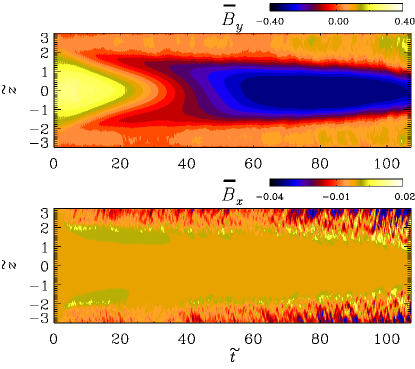
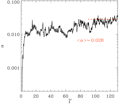
Figure 2: Left: spacetime diagrams of horizontally averaged mean magnetic fields, $\overline{B}_{y}$ (top) and $\overline{B}_{x}$ (bottom), which are normalized by $B_{\beta 1}$. Right: temporal behavior of the viscosity parameter $\alpha$. These are shown from the run A1s$\chi$ as listed in Table LABEL:tbl1.

3 Results

Results of our simulations that are summarised in Table LABEL:tbl1 are being presented here.

3.1 A1s$\chi$ Model

This is a large eddy simulation (LES) with a Smagorinsky viscosity in a shearing box. It covers about $\sim 110$ orbits. With $\beta_{0}=5.7$, initially imposed toroidal magnetic field is strong in this case, and therefore, the Parker-Rayleigh-Taylor-Instability (PRTI) is expected to be operational (Kadowaki et al, 2018). The run A2s as listed in Table LABEL:tbl1 has a slightly larger ${\rm Rm}$, but is otherwise similar to A1s$\chi$ model. Findings from these two runs are quite similar, so, below we present results from the run A1s$\chi$.

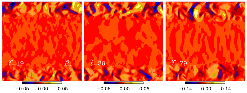
Figure 3: Three snapshots of the normalized vertical magnetic field ($\widetilde{B}_{z}$) from the $y=0$ plane from the run A1s$\chi$; see Table LABEL:tbl1 and Figure 2.

3.1.1 Vertical structure of disc-corona system

Figure 1 shows the vertical profile of the thermodynamic variables and the time evolution of volume average based root-mean-squared (rms) strengths of the fluid velocity ($u_{\rm rms}$) and total magnetic field ($B_{\rm rms}$) from the combined disc-corona system. As may be seen from Figure 1a, a temperature jump, with a corresponding drop in the density (not shown), in the corona by factor 10 compared to the disc is maintained during the simulation. Relaxation term in the entropy equation is applied only for the layers with $|\tilde{z}|\geq 2$. As time passes, we do observe a gradual drift of the transition layer in such a way that the extent of the corona increases. This is expected due to heating in the system by magnetic reconnection.

Thus we a have a piece-wise isothermal domains where a cold disc is embedded between coronal envelope of higher temperatue. System is vertically stratified under liner gravity which leads to correspondingly piece-wise Gaussian profiles for pressure as well as density in the disc and corona; see Figure 1b where $\tilde{z}=0$ is the midplane of the disc, and the pressure is continuous across the interface.

Turbulence is quickly produced within a few rotation time due to the magnetic field. Flow is subsonic and $u_{\rm rms}$ shows a saturation after about 20 rotation time. The simulation starts with an initial toroidal magnetic field $B_{y}$ which is Gaussian in structure with $\beta_{0}=5.7$. Figure 1d shows that $B_{\rm rms}$ decays in the beginning and after about 30 rotation times, it starts to grow. This growing phase is linked to the reversal of the toroidal magnetic field; see the paragraph below for a discussion on the reversal of $\overline{B}_{y}$. Both, the magnetic field and the turbulence, are maintained self-consistently in this system.

3.1.2 Reversal of toroidal magnetic field ($\overline{B}_{y}$)

Figure 2 shows the spacetime diagrams of the horizontally averaged mean magnetic fields, $\overline{B}_{y}$ (left, top) and $\overline{B}_{x}$ (left, bottom), which are normalized by $B_{\beta 1}$ defined earlier. Remarkably, the mean toroidal magnetic field undergoes a complete reversal in time by changing its sign, and it is predominantly confined within the disc. This is a rather unique class of evolution of the magnetic field which has not been reported earlier; see the spacetime diagrams in Figure 2, and in a number of other cases discussed below. The $x$-component of the mean magnetic field is mostly confined in the coronal regions, and it is generated by the MHD instabilities in this system.

Vertically migrating dynamo waves are commonly seen in a number of previous works which typically model an isothermal disc (Brandenburg et al, 1995; Simon, Beckwith & Armitage, 2012; Salvesen et al, 2016a; Kadowaki et al, 2018). The reversal of the toroidal magnetic field that we find in this work is quite intriguing. Unlike magnetic field solutions in an isothermal boxes considered in earlier works, we find here that the first moments of the magnetic fields, $\overline{B}_{x}$ and $\overline{B}_{y}$, are spatially separated. This is caused by the hot corona above the disc.

3.1.3 Vertical magnetic fields

In Figure 3 we show profiles of the unaveraged vertical magnetic fields from the snapshots taken at different times where we chose to display the structure from the $y=0$ plane. These fields are produced by the action of buoyancy effects in such stratified systems which are expected to host instabilities such as MRI and PRTI. As is evident from Figure 3, $B_{z}$ is predominantly confined in the low density coronal regions where it appears to be of small scale in nature and its strength increases in time.

3.1.4 Viscosity parameter ($\alpha$)

Time evolution of the Shakura-Sunyaev (SS) viscosity parameter ($\alpha$) as defined below Eq. (11) is shown in the right panel of Figure 2. We find that $\alpha$ saturates with a mean value of $\sim 0.03$ after about 50 rotation times. This is about ten times larger compared to the value of $\alpha$ obtained in Brandenburg et al (1995), and close to the one seen in simulations of Kadowaki et al (2015).

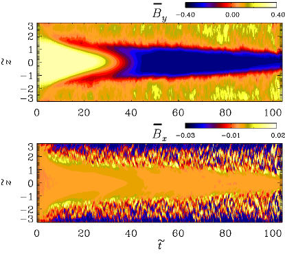
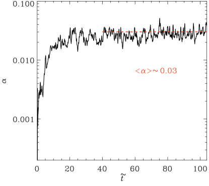
Figure 4: Same as Figure 2 but from the run B1e listed in Table LABEL:tbl1.

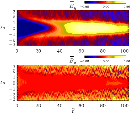
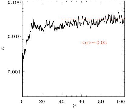
Figure 5: Same as Figure 2 but from the run “B1eN” (not listed in Table LABEL:tbl1) which is identical to the run B1e of Table LABEL:tbl1, except that the initial $B_{y}$ in this case has the opposite sign.

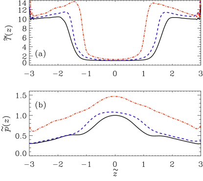
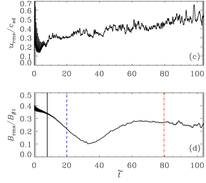
Figure 6: Same as Figure 1 but from the lower resolution run “B1eN”; see the caption of Figure 5.

3.2 Comparison between models with different numerical schemes for kinematic viscosity ($\nu$)

In order to test how sensitive are our results to the numerical schemes adopted for $\nu$, we perform another set of simulations with explicit kinematic viscosity. One such run, called A3e in Table LABEL:tbl1, is presented in this work; see Appendix A where we include results from this run with explicit $\nu$. Note that this has smaller ${\rm Rm}$ (and ${\rm Re}=78$) compared to the A1s$\chi$ model with Smagorinsky viscosity discussed above in Sect. 3.1. Broad conclusions from models with these two different numerical schemes for $\nu$ are same, i.e., the toroidal magnetic field undergoes a complete reversal as discussed in Sect. 3.1. Further discussion on this deferred to Appendix A.

3.3 Models with $\beta_{0}=1.5$ and oppositely directed initial magnetic field configurations

Here we present results from two lower resolution runs, B1e (listed in Table LABEL:tbl1), and B1eN which is identical to the run B1e, except that the initial $B_{y}$ in this case has the opposite sign. We have used explicit $\nu$ in both these cases where we test the robustness of our findings discussed above on the field reversals. In Figures 4 and 5 we show the spacetime diagrams of mean magnetic fields, $\overline{B}_{x}$ and $\overline{B}_{y}$, as well as the time evolution of the SS viscosity parameter $\alpha$. Mean toroidal field $\overline{B}_{y}$ undergoes a complete reversal in time by changing its sign in both these cases, and the SS viscosity parameter $\alpha$ saturates to a mean value of $\sim 0.03$ after about 30 rotation times.

As may be seen from Figure 6(a), there is a gradual drift of the disc-corona interface also in these cases such that the extent of hotter corona slowly increases. Recall that the relaxation term, as discussed in Sect. 2, to maintain the corona of higher (lower) temperature (density) is applied only in layers with $|\tilde{z}|\geq 2$. Figure 6(c) shows that the instabilities in the magnetized disc drive turbulence, which, in turn, governs the evolution of magnetic field in a self-sustaining manner. Ohmic heating due to magnetic reconnection of small scale loop-like structures which are prominant in the low density coronal regions is likely the cause for further heating of corona. This is expected to play a crucial role in the formation of corona in the magnetized accretion discs.

3.4 A discussion on the run C1s in a tall box

We have also performed some simulations in a tall box where the vertical extent is four times larger than the horizontal extents; $\tilde{z}\in[-4,4]$ with relaxation term to maintain the corona operating in $|\tilde{z}|\geq 2$ layers. Corona is therefore thicker compared to the cubic domains considered in cases above. Due to piece-wise isothermal setups that are vertically stratified under linear gravity being studied in this work, the densities become vanishingly small in top layers of corona in such tall boxes. This leads to numerical challenges and increases the computational cost of such models. Nevertheless, some early findings from this run seem interesting enough, so we mention them briefly here without showing any plots from this run.

As in other cases discussed above, the run begins with a toroidal field $B_{y}$ with a Gaussian profile along $\tilde{z}$ such that the initial $\beta_{0}=3.4$ is constant in $\tilde{z}$. Buoyancy instabilities such as PRTI lead to the generation of other components of magnetic fields in a manner similar to the one discussed in Kadowaki et al (2018). Corona acts as a reservoir of small-scale loop-like magnetic fields, especially the $B_{z}$. Ohmic heating due to magnetic reconnection as studied by Kadowaki et al (2018) is expected to be more efficient in this run with a thicker corona. As we enforce a constant temperature at the vertical boundaries determined through the relaxation term in Eq. (3), the excess heat produced is therefore pushed towards the cool disc. This makes the combined system asymptotically isothermal over $\sim 100$ rotation times. The resulting solutions for the mean magnetic fields, $\overline{B}_{x}$ and $\overline{B}_{y}$, thus display the well known vertically migrating butterfly patters found in a number of previous works (Brandenburg et al, 1995; Simon, Beckwith & Armitage, 2012; Salvesen et al, 2016a; Kadowaki et al, 2018).

4 Discussion & Conclusions

The geometrically thin gas pressure dominated accretion disc cannot completely explain the phenomenology of accretion disc around compact objects such as X-ray Binaries and AGNs (Mishra et al, 2020). Thermo-viscous instabilities and high energy spectral characteristics from these sources indicate that hot geometrically thick and magnetised component of accretion flow is also present (Gaburov, Johansen & Levin, 2012; Begelman & Pringle, 2007). Magnetic energy dissipation is the main internal mechanism of heating of the disc except the irradiation by very inner part of the accretion disc. There are several attempts to explain the self-sustained generation of large scale magnetic field in accretion around compact objects. It is argued that even if the system starts with a very week magnetic field, strong toroidal magnetic field could be sustained in a later phase (Kudoh et al, 2002; Pessah & Psaltis, 2005) driven by MRI (Miller & Stone, 2000; Kadowaki et al, 2015; Begelman et al, 2015). In our work we choose such an initial organised toroidal magnetic field (Begelman & Pringle, 2007), which is superposed on a preexisting cold disc – hot corona, as discussed in the introduction.

Main results of this work can be summarised as follows:

1. The cold disc-hot corona vertical temperature profile is stable: in all the simulations the symmetric step profile of the temperature as a function of vertical coordinate is maintained. Results are independent of Smagorinsky or explicit scheme for the kinematic viscosity.

2. Instabilities in the magnetized disc drive turbulence, which, in turn, governs the evolution of magnetic field in a self-sustaining manner.

3. The large scale toroidal magnetic field is largely confined to the cold disc region: contrary to the general belief, in cold disc-hot corona system, the large scale toroidal magnetic field is strong in the disc region and weakens in the corona region. It is found that the system suppresses the magnetic buyount force, confining the large scale toroidal magnetic field in the disc region.

4. Remarkably, the mean toroidal magnetic field undergoes a complete reversal in time by changing its sign, and it is predominantly confined within the disc. This is a rather unique class of evolution of the magnetic field which has not been reported earlier. Toroidal magnetic field thus shows an aperiodic field reversal.

   Vertically extended shearing box simulations in other works where an isothermal gas is modeled, one typically finds dynamo waves, i.e., a butterfly pattern for mean fields which show quasi-periodicity over time scales on the order of 10 rotation times. In our case with a piece-wise isothermal disc-corona system, we find that the toroidal fields reverses over a time scale of the order of $50$ rotation times, and the commonly seen butterfly pattern of the dynamo wave is absent.

5. Saturated value of the SS viscosity parameter $\alpha$ is about $0.03$ for several tens of rotation times. This is in conformity with most of the shearing box simulations of magnatised accretion disc. The Maxwell’s stress is found to be stronger than Reynold’s stress and it largely contributes to $\alpha$.

Thermal Comptonization (Shapiro, Lightman & Eardley, 1976; Sunayev & Titarchuk, 1980) in the hot and low dense corona is generally invoked to explain the high energy emission. Apart from the continuous corona, distinct active regions of coronal clouds above the disc are also suggested in this context (Haardt, Maraschi & Ghisellini, 1994). In a magnetically coupled disc-corona system, the interaction could cause further increase of the coronal temperature (Merloniw & Fabian, 2001; Kuneida et al, 1990; Zdziarski, 1990; Haardt & Maraschi, 1991). The amplification of seed magnetic field in disc by differential rotation and convection is generally balanced by microscopic diffusivities. In a gravitationaly stratified gas, a horizontal magnetic field can trigger unstable modes leading to Parker instability (Parker, 1958, 1966). In an isothermal setup if the magnetic field cannot dissipate at the rate of amplification then magnetic field could emerge from the disc to coronal region due to buoyoncy and magneric loops could dissipate in the coronal region (Galeev, Rosner & Vaiana, 1979).

Differentially rotating systems such as disc galaxies show magnetic field reversals while moving radially (Vallee, 1996; Frick et al, 2001; Van Eck et al, 2011). Mechanisms such as turbulent dynamo effect and stellar feedback are involved to understand the evolution of magnetic fields in these systems (Brandenburg et al, 2015; Kotarba et al, 2009). Fully isothermal, shearing box simulations to model accretion discs reveal a butterfly pattern where the dynamo wave leads to a quasi-periodicity in mean magnetic fields with a period of about 10 rotation time (Brandenburg et al, 1995; Kadowaki et al, 2015; Salvesen et al, 2016a; Kadowaki et al, 2018). Whereas in our two-layer system of cool disc and a hot corona, the quasi-periodicity of mean fields as found in earlier works is absent. Instead, the mean toroidal magnetic field undergoes a complete reversal over a time scale of about 50 rotation by changing its sign, and it is predominantly confined within the disc.

Interaction of a hot corona on top of a cool disc was invoked in the context of the so called slab model to explain thermal Comptonized X-rays from the disc (Dove et al, 1997, 2000). Observations in Black Hole Binaries and AGN’s show that the fraction of total energy dissipated in corona is very large (Haardt & Maraschi, 1991; Petrucci et al, 2018). Magnetically supported steady state accretion disc corona models with active MRI (Gronkiewicz & Różańska, 2019) also suggest that an appreciable amount of energy release could happen in the corona region.

As noted above, $\overline{B}_{y}$ is largely confined to the disc region due to the presence of a hot corona above. Whereas $\overline{B}_{x}$, and also $B_{z}$ are prominent in the corona; see Sect. 3.1. We envisage that Ohmic heating due magnetic reconnection of smaller scale field structures will be more efficient in the coronal region, producing thus an excess heat which may heat-up the disc. Corona thus ‘advances’ towards the disc, swallowing the matter from the disc to facilitate more efficient accretion of the matter. This particular situation could creates a scenario of accretion via corona.

Appendix A Field reversals in runs with explicit kinematic viscosity

Here we show results from the run A3e listed in Table LABEL:tbl1, where we adopt an explicit diffusion scheme for the kinematic viscosity ($\nu$), to demonstrate that the results presented in Sect. 3 are robust. In Figure 7, we show the vertical profiles, and the temporal evolution, of the thermodynamic variables. Also shown are the time dependence of $u_{\rm rms}$ and $B_{\rm rms}$. The sharp transition between the cool disc and the hot corona by the relaxation term in Eq. (3) is better maintained in time in this case. Recall that, just like the other cases discussed in this work, the run begins with a toroidal field $B_{y}$ with a Gaussian profile along $\tilde{z}$ such that the initial $\beta_{0}=5.7$ is constant within the disc.

From Figure 7(c) and (d) we note that, while the $B_{\rm rms}$ evolves smoothly as in Figure 1 for the A1s$\chi$ model, $u_{\rm rms}$ shows an outburst like activity in time. This leads to an interesting, burst-like temporal evolution of the SS viscosity parameter $\alpha$ as shown in the right panel of Figure 8. Peak value of the $\alpha$ exceeds the value 0.01 which is consistent with our findings as presented in Sect. 3, and also with the values reported in some other works discussed before.

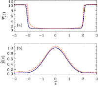
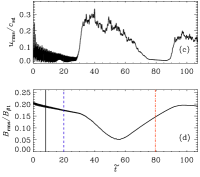
Figure 7: Same as Figure 1 but from the run A3e as listed in Table LABEL:tbl1.

Spacetime diagrams of mean magnetic fields, $\overline{B}_{x}$ and $\overline{B}_{y}$, as shown in Figure 8 reveal the reversal of toroidal component which is strongest in the disc region, whereas $\overline{B}_{x}$ is strong in the coronal regions. This is consistent with the results presented in Sect. 3 where a number of cases with Smagorinsky scheme for $\nu$ also show a similar pattern. Results presented in this work are thus independent of the numerical schemes for kinematic viscosity. Burst-like behavior of the SS viscosity parameter $\alpha$ in time may have interesting consequences for accretion pattern and may help us better understand the observations. In future work, we will focus more on this by performing simulations at larger Reynolds numbers.

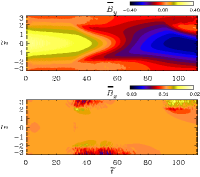
Figure 8: Same as Figure 2 but from the run A3e as listed in Table LABEL:tbl1.

References

- Abramowicz et al (1995) Abramowicz, M. A., Chen, X., Kato, S., Lasota, J.-P., & Regev, O. 1995, ApJL, 438, L37
- Abramowicz & Fragile (2013) Abramowicz, M. A., & Fragile, P. C. 2013, LRR, 16, 1
- Bagnoli et al (2015) Bagnoli, T., in ’t Zand, J. J. M., D’Angelo, C. R., Galloway, D. K., MNRAS, 2015, 449, 268
- Bai & Stone (2013) Bai, X. N., & Stone, J. M. 2013, ApJ, 767, 30
- Balbus & Hawley (1998) Balbus, S. A., & Hawley, J. F. 1998, RvMP, 70, 1
- Balbus & Hawley (1991) Balbus, S. A., & Hawley, J. F. 1991, ApJ, 376, 214
- Begelman & Pringle (2007) Begelman, M. C & Pringle, J. E, 2007, MNRAS, 375, 1070
- Begelman et al (2015) Begelman M. C., Armitage P. J. & Reynolds C. S., 2015, ApJ, 809, 118
- Belloni (2010) Belloni, T. M in Jet paradigm, Lecture Notes in Physics 2010, Springer
- Belloni et al (2005) Belloni, T., Homan, J., Casella, P., et al. 2005, A&A, 440, 207
- Belloni & Motta (2016) Belloni, T. M., & Motta, S. E. 2016, in Astrophysics of Black Holes (Berlin, Heidelberg: Springer-Verlag), Astrophys. Space Sci. Lib., 440, 61
- Blandford & Begelman (1999) Blandford, R. D., & Begelman, M. C. 1999, MNRAS, 303, L1
- Bosch-Ramon, Aharonian & Paredes (2005) Bosch-Ramon, V., Aharonian, F. A., & Paredes, J. M. 2005, A&A, 432, 609
- Brandenburg et al (1995) Brandenburg, A., Nordlund, A., Stein, R. F., & Torkelsson, U. 1995, ApJ, 446, 741
- Brandenburg et al (2015) Brandenburg A., 2015, in Lazarian A., de Gouveia Dal Pino E. M., Melioli C., eds, Astrophysics and Space Science Library Vol. 407, Astrophysics and Space Science Library. p. 529
- Chandrasekhar (1960) Chandrasekhar, S. 1960, PNAS, 46, 253
- Davis, Stone & Pessah (2010) Davis, S. W., Stone, J. M., & Pessah, M. E. 2010, ApJ, 713, 52
- de Gouveia Dal Pino & Lazarian (2005) de Gouveia Dal Pino, E. M., & Lazarian, A. 2005, A&A, 441, 845
- de Gouveia Dal Pino et al (2010) de Gouveia Dal Pino, E. M., Piovezan, P. P., & Kadowaki, L. H. S. 2010, A&A, 518, 5
- Dove et al (2000) Dove, J. B., Wilms, J., & Begelman, M. 2000, ApJ, 999, L1 - L14
- Dove et al (1997) Dove, J. B., Wilms, J., Maisack, M, & Begelman, M. 2000, ApJ, 999, L1 - L14
- Fender, Belloni & Gallo (2004) Fender, R. P., Belloni, T. M., & Gallo, E. 2004, MNRAS, 355, 1105
- Frick et al (2001) Frick P., Stepanov R., Shukurov A., Sokoloff D., 2001, MNRAS, 325, 649
- Gaburov, Johansen & Levin (2012) Gaburov E., Johansen A., Levin Y., 2012, ApJ, 758, 103
- Galeev, Rosner & Vaiana (1979) Galeev, A., Rosner, R. & Vaiana, G. S. 1979, ApJ, 229, 318-326
- Giveon, Maoz et al (1999) Giveon U., Maoz D., Kaspi S., Netzer H., Smith P., 1999, MNRAS, 306, 637
- Gronkiewicz & Różańska (2019) Gronkiewicz, D. & Różańska, A. 2019, A&A, 633, A35, 17
- Gutiérrez, Vieyro & Romero (2021) Gutiérrez, E. M , Vieyro, F. L & Romero, G. E, 2021, A & A 649, A87
- Haardt & Maraschi (1991) Haardt, F., & Maraschi, L. 1991, ApJ, 380, L51
- Haardt, Maraschi & Ghisellini (1994) Haardt F., Maraschi L. & Ghisellini G., 1994, ApJ, 432, L95
- Haugen & Brandenburg (2006) Haugen, N. E. L., & Brandenburg, A., 2006, Phys. Fluids, 18, 075106
- Hawley, Gammie & Balbus (1995) Hawley, J. F., Gammie, C. F., & Balbus, S. A. 1995, ApJ, 440, 742
- Hirose, Krolik & Stone (2006) Hirose S., Krolik J. H.& Stone J. M., 2006, ApJ, 640, 901
- Huang, Wu & Wang (2014) Huang, C. Y., Wu, Q., & Wang, D.X. 2014, MNRAS, 440, 965
- Igumenshchev & Abramowicz (1999) Igor V. Igumenshchev & Marek A. Abramowicz 1999, MNRAS 303, 309–320
- Inoue et al (2019) Inoue, Y., Khangulyan, D., Inoue, S., & Doi, A. 2019, ApJ, 880, 40
- Ishibashi & Courvoisier (2009) W. Ishibashi , T. J.-L. Courvoisier A & A 2009,504, 61 -66
- Lasota (2001) Lasota J.-P., 2001, New. Astron. Rev., 45, 449
- Lasota (1999) Lasota, J.-P., 1999, in: S. Mineshige, J.C. Wheeler (Eds.), Disk Instabilities in Close Binaries - 25 years of the Disk Instability Model, Universal Academy Press, Tokyo, p. 191
- Lewin & van der Klis (2006) Lewin W., van der Klis M., 2006, Compact Stellar X-ray Sources. Cambridge Univ. Press, Cambridge
- Liu, Mineshige & Ohsuga (2003) Liu, B. F., Mineshige, S., & Ohsuga, K. 2003, ApJ, 587, 571
- Liu et al (2015) Liu, B. F., Taam, R., Qiao, E., et al. 2015, ApJ, 806, 223
- Macioøek-NiedzÂwiecki, Krolik & Zdziarski (1997) Macioøek-NiedzÂwiecki A., Krolik J. H. & Zdziarski A. A., 1997, ApJ, 483,111
- Merloniw & Fabian (2001) Merloniw, A & Fabian, A. C., 2001 MNRAS, 321, 549
- Meyer-Hofmeister, Liu & Qiao (2017) Meyer-Hofmeister, E., Liu, B. F. & Qiao, E., 2017 A&A 607, A94
- Meyer, Liu & Meyer-Hofmeister (2000) Meyer, F., Liu, B. F., & Meyer-Hofmeister, E. 2000, A&A, 361, 175
- Miller & Stone (2000) Miller, K. A., & Stone, J. M. 2000, ApJ, 534, 398
- Mishra et al (2020) Mishra, B., Begelman, M. C., Armitage, P. J. & Simon, J., B., 2020, MNRAS, 492, 1855
- Narayan & Yi (1994) Narayan, R., & Yi, I. 1994, ApJL, 428, L13
- Narayan & Yi (1995) Narayan, R., & Yi, I. 1995, ApJ, 452, 710
- Novikov & Thorne (1973) Novikov, I. D., & Thorne, K. S. 1973, Black Holes (Les Astres Occlus) (NY:Gordon and Breach), 343
- Paradijs & McClintock (1995) Paradijs J., McClintock J.E., 1995, in Lewin W.H.G., van Paradijs J., van den Heuvel E.P.J., eds., X-ray Binaries. Cambridge University Press, Cambridge, p. 58
- Parker (1958) Parker, E. N., 1958, Phys. Rev., 109, 1328
- Parker (1966) Parker E. N., 1966, ApJ, 145, 811
- Petrucci et al (2018) Petrucci, P. O., Ursini, F., De Rosa, A., et al. 2018, A&A, 611, A59
- Pessah & Psaltis (2005) Pessah, M. E & Psaltis, D, 2005, ApJ, 628, 879
- Pica, Smith et al (1988) Pica A. J., Smith A. G., Webb. J. R., Leacock R. J., Clements S., Gombola P. P., 1988, AJ, 96, 1215
- Piano et al (2012) Piano, G., Tavani, M., Vittorini, V., et al. 2012, A&A, 545, A110
- Pringle (1981) Pringle, J. E. 1981, ARA&A, 19, 137
- Qiao & Liu (2017) Qiao, E., & Liu, B. F. 2017, MNRAS, 467, 898
- Remillard & McClintock (2006) Remillard R. A, McClintock J. E, ARA&A, 44,49, 2006
- RoÂzÇanÂska & Czerny (1996) RoÂzÇanÂska A. & Czerny 1996, Acta Astronomica, 46,233
- RoÂzÇanÂska (1999) RoÂzÇanÂska A., MNRAS, 1999, 308, 751
- Romero et al (2003) Romero, G. E., Torres, D. F., Kaufman Bernadó, M. M., & Mirabel, I. F. 2003, A&A, 410, L1
- Różańska & Czerny (2000) Różańska, A., & Czerny, B. 2000, MNRAS, 316, 473
- Salvesen et al (2016a) Salvesen, G., Simon, J. B., Armitage, P. J., & Begelman, M. C. 2016, MNRAS, 457, 857
- Salvesen et al (2016b) Salvesen, G., Armitage, P. J., Simon, J. B., & Begelman, M. C. 2016, MNRAS, 460, 3488
- Sartori et al (2018) Sartori, L. F., Schawinski, K., et al. 2018, MNRAS Letters, 476, L34–L38
- Shakura & Sunyaev (1973) Shakura, N. I., & Sunyaev, R. A. 1973, A&A, 500, 33
- Shapiro, Lightman & Eardley (1976) Shapiro S. L., Lightman A. P., Eardley D. M., 1976, ApJ, 204, 187
- Simon, Beckwith & Armitage (2012) Simon, J. B., Beckwith, K., & Armitage, P. J. 2012, MNRAS, 422, 2685
- Smak (2000) Smak, J, New Astronomy Review, 2000, 44, 171
- Sunayev & Titarchuk (1980) Sunayev R. A. & Titarchuk L. G., 1980, A&A, 86, 121
- Kadowaki et al (2015) Kadowaki, L. H. S., de Gouveia Dal Pino, E. M., & Singh, C. B. 2015, ApJ, 802, 113
- Kadowaki et al (2018) Kadowaki, L. H. S., de Gouveia Dal Pino, E. M., & Stone, J. M. 2018, ApJ, 864:52
- Käpylä (2021) Käpylä, P. J. K., 2021, A&A, 655, A78
- King & Ritter (1998) King A. R. & Ritter H., 1998, MNRAS, 293, L42
- King, Pringle & Livio (2007) King, A. R, Pringle, J. E. & Livio, 2007, MNRAS, 376, 1740
- Kudoh et al (2002) Kudoh, T., Matsumoto, R., & Shibata, K. 2002, PASJ, 54, 121
- Kuneida et al (1990) Kuneida, H., Turner, T. J., Awaki, H., Koyama, K., Mushotzky, R. F & Tsusaka, Y. 1990, Nature, 345,786
- Kotarba et al (2009) Kotarba H., Lesch H., Dolag K., Naab T., Johansson P. H., Stasyszyn F. A., 2009, MNRAS, 397, 733
- Kylafis & Belloni (2015) Kylafis, N. D., & Belloni, T. M. 2015, A&A, 574, A133
- Vallee (1996) Vallee, J, P. 1996, A&A, 308, 433
- Van Eck et al (2011) Van Eck C. L., et al., 2011, ApJ, 728, 97
- van Paradijs & Mc Clintock (1994) van Paradijs J., Mc Clintock J. E., 1994, A & A, 290, 133
- Warner (2003) Warner B., 2003, Cataclysmic Variable Stars. Cambridge Univ. Press, Cambridge
- Winters, Balbus & Hawley (2003) Winters W. F., Balbus S. A. & Hawley J. F., 2003, ApJ, 589, 543
- Wojaczyński et al (2015) Wojaczyński, R., Niedźwiecki, A., Xie, F.-G., & Szanecki, M. 2015, A&A, 584, A20
- Yuan (2001) Yuan, F. 2001, MNRAS, 324, 119
- Yuan & Narayan (2014) Yuan, F., Narayan, R 2014, ARA & A, 52, 529
- Zdziarski (1990) Zdziarski, A. A., Ghisellini, G., George, I. M., Fabian, A. C, Svensson, R & Done, C. 1990, ApJ, 363, LI