The application of Hough transform for fast interaction vertex position estimation in heavy-ion collisions

Abstract

Track reconstruction in high-multiplicity events, such as heavy-ion collisions at LHC, is a difficult and resource-demanding process. A priori knowledge of the collision vertex position would allow discarding non-viable track seeds, reducing the overall computing requirements for the track reconstruction. The method proposed in this note uses the Hough transform for the estimation of the interaction vertex position without the necessity to reconstruct the tracks first. It offers admissible resolution with linear scaling of numerical complexity with the track multiplicity.

Keywords: Hough transform; heavy-ion collisions; linear complexity; track reconstruction; vertex reconstruction

1 Introduction

Ultrarelativistic heavy-ion collisions, such as those occurring at the LHC, generate a large number of charged particles. In ultra-central collisions, the number of charged particles produced in a single collision can reach a couple thousand per pseudorapidity unit [1, 2, 3]. Reconstruction of the trajectories of these charged particles from measurements in the detector is a time-consuming process. The required time is a non-linear function of a number of signals and can be as high as several hours per event if reconstruction of low transverse momenta (e.g. 100 MeV) of particles is needed. The first stage of reconstruction involves the generation of the so-called seeds, measurement triplets, from the measurements left by particles in the detector layers [4]. During seed generation, no assumption on vertex position along the $z$-axis is made.

Knowing the vertex $z$-position, even approximately, would allow us to consider only seeds originating from that estimated vertex. Such a constraint would significantly reduce the number of seeds to examine and thus accelerate the reconstruction process. Previously suggested algorithms use combinations of detector hits (doublets or triplets) to generate vertex position estimates [5]. The drawback of this approach is that the algorithm’s complexity is polynomial as a function of the number of measurements.

The approach suggested here employs the Hough transform (HT) [6] and has a linear complexity as a function of the number of measurements. The studies of this method are performed using ACTS toolkit [4] based on ODD detector model [7], a simplified version of silicon tracking detectors to be used by the LHC experiments in High-Luminosity LHC phase [8, 9, 10]. The Pb+Pb events are generated using Pythia Angantyr heavy-ions collision model [11] at centre-of-mass energy per nucleon $\sqrt{s_{{}_{\rm NN}}}=5$ TeV.

2 Method

In high-energy physics experiments, two types of tracking detectors are typically used: pixel detectors and strip detectors. Each type has specific advantages and is utilised based on the requirements of the experiment. The proposed algorithm demands precise information about the $z$-position of the measurements and thus is only applicable with pixel detectors. Also, it can only be applied in case of a uniform magnetic field aligned with the direction of the colliding beams and the $z$ axis or the absence of the field.

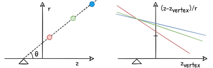
Figure 1: Sketch of the Hough transform. Left: The red, green, and blue measurements originate from the same particle whose trajectory forms an angle $\theta$ with the $z$-axis. The vertex of origin is denoted by a triangle. Right: The same measurements are translated into lines in the Hough image space. They cross each other at the $z_{vertex}$ position of their origin.

First, the measurement coordinates are transformed into a Hough image space using the formula:

$$\cot(\theta)=(z_{m}-z_{vertex})/r_{m},$$ (1)

where $z_{m}$ and $r_{m}$ are cylindrical coordinates of a measurement, $z_{vertex}$ is the vertex position, and $\theta$ is the angle between the particle and the $z$-axis. Usage of $\cot(\theta)$ instead of $\theta$ reduces the computation to a single multiplication and addition per measurement per $z_{vertex}$, making the computation very efficient.

Figure 1 illustrates the construction of such an image space for three measurements. In a collision with many particles originating from the same vertex, the $\theta$ angles and consequently the $\cot(\theta)$ values would differ from particle to particle, yet the $z_{vertex}$ position would be common.

Then, in line with typical HT implementations, the image space is quantised into a 2D histogram, and its bins are filled if coincident with the line corresponding to each measurement. Then, the bins of the histogram undergo a pedestal removal procedure. This process retains only the bins with a sufficient count of intersecting lines, enhancing the signal/background ratio of the image space. After the pedestal removal, the histogram is integrated along the $\cot(\theta)$ dimension, transforming the image into a 1D histogram with a distinct peak.

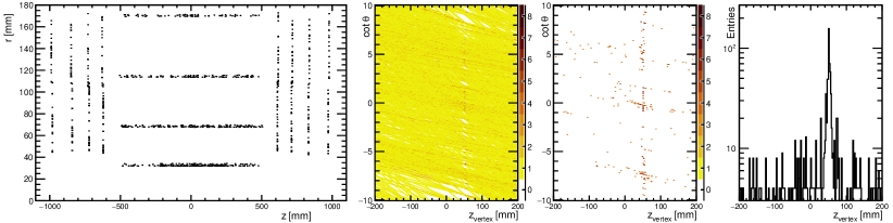
Figure 2: Example of the vertex estimation. From the left: Detector measurements projected into the $r$–$z$ space; Hough image space; Hough image space after the pedestal removal procedure; and 1D projection of the image space along the $\cot(\theta)$ dimension.

An example of this process is shown in Figure 2 for an event with moderate particle multiplicity and a generated vertex at $z=50.9\,\text{mm}$. In this case, the initial image space might not show any evident pattern before pedestal removal. After the pedestal removal, a clear pattern emerges, which becomes even more pronounced in the 1D projection.

3 Evaluation and algorithm parameters

The algorithm’s effectiveness is measured by the resolution of the estimated vertex position. The algorithm shall perform equally effectively for events with large differences in occupancy, as is the case in heavy-ion collisions.

The performance of the algorithm depends on several parameters: (a) the selection of the measurements considered for each $z_{vertex}$; (b) granularity of the binning in the $\cot(\theta)$ dimension; (c) filling scheme for the image histogram; (d) the threshold on the number of entries in the image space in the pedestal removal procedure. Optimal selection of these parameters is crucial for the overall algorithm performance. The effect of modifying the parameters on the 1D projection of the image space is shown in Figure 3.

An option to consider only part of the measurements was studied, to mitigate overpopulation of the image space in the more central events. The set of measurements used for a given $z_{vertex}$ hypothesis is constrained to a range in the angle around it (defined using $\eta=\text{arcsinh}[\cot(\theta)]$). An effect of constraining the $|\eta|$ range is shown in the leftmost panel of Figure 3. A wide range (large $|\eta|$ values) in high-occupancy events leads to an overpopulation of the image histogram, precluding the peak finding. On the contrary, a too-narrow range may result in the absence of a peak for events of small occupancy.

Another approach to tame the occupancy of the image histogram is to change its granularity along the $\cot(\theta)$ axis, as shown in the second panel of Figure 3. Finer granularity may prevent the formation of the peak in low-multiplicity events, but coarser granularity may result in overpopulation in high-multiplicity events.

The combined effect of adapting the $\cot(\theta)$ binning and $|\eta|$ range is illustrated in the third panel of Figure 3. As exemplified, a fixed granularity per unit of $\cot(\theta)$ preserves a peak for diverse kinds of events.

In experimental reality, the tracks do not form perfect trajectories due to scattering effects. Consequently, the bins in the HT image space must be sufficiently broad to accommodate this effect, which on the other hand would deteriorate the performance in the event of high occupancy. To recover the “near-miss” entries in the peak, the line corresponding to each measurement is widened, i.e. the adjacent bins in $\cot(\theta)$ are also filled. The fourth panel of Figure 3 shows the effect of such width expansion for events of different occupancy. For very low occupancy events, this procedure helps to identify the peak, while for “bussier” events it obscures the solution.

The impact of the threshold value in the pedestal removal step is shown in the rightmost panel of Figure 3. Requiring a high count per bin improves the significance of the peak in events with high occupancy; however, a too-high value results in suppression of the peak in events with lower occupancy.

Last but not least, to ensure practical implementation, the design of the algorithm must consider the memory required to store the HT image space histogram. To save both memory and computational time, the algorithm can be run multiple times, with increasing granularity (i.e. bins per mm) and decreasing range along the $z$-axis.

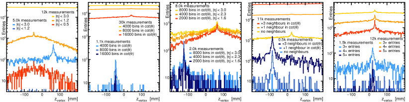
Figure 3: Effects of the different parameter setups. From the left: Considered $|\eta|$ range of the measurements; number of bins along $\cot(\theta)$ axis; number of bins along the $\cot(\theta)$ axis and considered $|\eta|$ range such that the amount of bins per unit of $\cot(\theta)$ remains the same; filling more bins in the HT image space along the $\cot(\theta)$ axis; and a minimum number of entries per bin in the HT image space. Unless stated otherwise in the legend, the algorithm considers $|\eta|<3.0$, has 8000 bins along the $\cot(\theta)$ axis, requires at least 4 entries per bin, and does not fill any neighbouring bins.

The following set of parameters was tuned to the ODD detector and is used to evaluate the algorithm performance discussed in Section 4. If there are more than $10^{4}$ measurements in $|\eta|<3.0$, then the $|\eta|$ range is limited, so the utilised number of measurements remains close to $10^{4}$. The expectations are based on the average distribution of measurements along $|\eta|$. This limitation prevents over-population of the HT image; setup of other parameters wages against the resolution deterioration at lower-multiplicity events. If there are at least $10^{4}$ measurements, then the $\cot(\theta)$ axis has 8000 bins. For fewer measurements, the number of bins is reduced by $2^{4-\log_{10}\left(N_{m}\right)}$, where $N_{m}$ is the number of measurements. Moreover, if there are less than 1000 (200) measurements, then 1 (3) neighbours in $\cot(\theta)$ are filled as well. The pedestal removal procedure requires at least 4 entries per bin. The algorithm is run three times: with 800 bins in $|z_{vertex}|<200$ mm, with 180 bins in $|z^{\prime}_{vertex}-z_{vertex}|<30$ mm, and with 80 bins in $|z^{\prime\prime}_{vertex}-z_{vertex}|<8$ mm.

4 Performance

With the parameters optimised as described above, the performance was evaluated in 250k Pb+Pb events generated using Pythia Angantyr heavy-ions collision model [11] with collision vertices chosen at random following the Gaussian distribution centred at $(x,y,z)=(0,0,0)$ mm and width $(\sigma_{x},\sigma_{y},\sigma_{z})=(0.5,0.5,50)$ mm.

The efficiency of finding a vertex is studied and is found to be precisely 100%. The leftmost panel of Figure 4 shows the correlation between the generated and reconstructed vertex positions. All event multiplicities are combined in this figure. An excellent correlation is found between these two quantities.

The resolution, defined as the mean of a difference between the generated and reconstructed vertices in the $z$-direction, $\Delta z=|z_{vertex}^{reco}-z_{vertex}^{gen}|$, is shown for three event multiplicities as a function of the vertex $z$-position, $r$-position, and the measurement multiplicity is shown in the three right panels of Figure 4.

The resolution is flat along the $z$-axis. This is expected as the algorithm is agnostic about the $z_{vertex}$ position. Some deterioration at large $|z_{vertex}|$ may come from the detector design, though. For the $r$-position, the resolution worsens with increasing $r_{vertex}^{gen}$ because the algorithm assumes $(x_{vertex}^{gen},y_{vertex}^{gen})=(0,0)$ without any attempt to take such bias into account. Finally, the resolution is better for high-multiplicity events, as the peak finding performs better on smoother 1D histograms.

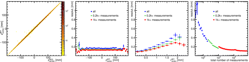
Figure 4: Performance of the algorithm. From the left: Correlation between reconstructed and generated $z$-positions of the vertices; resolution as a function of generated position along the $z$-axis and along the $r$-axis; and resolution as a function of measurements multiplicity in the event.

5 Summary

The algorithm using the Hough transformation for fast vertex estimation has been presented. The numerical complexity of the algorithm is linear as a function of measurements for a wide range of charged-particle multiplicities and becomes sublinear for high-multiplicity events. For the ODD detector, the position estimate resolution is about 1 mm for events with as little as 30 measurements; for events with more than 1000 measurements, the resolution is about $0.2$ mm. Similar performance is expected to be achieved for other detector designs.

To negate the performance degradation with increasing $r^{gen}_{vertex}$, it might be possible to run the algorithm iteratively with different assumptions of $(x_{vertex}^{gen},y_{vertex}^{gen})$ and estimate the correctness of each assumption from the size or shape of the peak in the 1D projection of the HT image space.

Although events with multiple vertices were not investigated, it might be possible to detect more vertices from the 1D projection, assuming the binning along the $z$-axis is fine and the vertices are separated well enough. Moreover, the magnitude of the peak in the 1D projection might be an efficient estimate of overall event multiplicity usable in online filtering applications.

References

- [1] ALICE Collaboration, Centrality Dependence of the Charged-Particle Multiplicity Density at Midrapidity in Pb-Pb Collisions at TeV, Phys. Rev. Lett. 116 no. 22, (2016) 222302, arXiv:1512.06104 [nucl-ex].
- [2] ATLAS Collaboration, Measurement of the centrality dependence of the charged particle pseudorapidity distribution in lead-lead collisions at TeV with the ATLAS detector, Phys. Lett. B 710 (2012) 363–382, arXiv:1108.6027 [hep-ex].
- [3] CMS Collaboration, Pseudorapidity distributions of charged hadrons in xenon-xenon collisions at TeV, Phys. Lett. B 799 (2019) 135049, arXiv:1902.03603 [hep-ex].
- [4] X. Ai et al., A Common Tracking Software Project, Comput. Softw. Big Sci. 6 no. 1, (2022) 8, arXiv:2106.13593 [physics.ins-det].
- [5] N. P. Konstantinidis and H. Drevermann, Determination of the z position of primary interactions in ATLAS, ATL-DAQ-2002-014 (2002).
- [6] P. V. C. Hough, Machine Analysis of Bubble Chamber Pictures, Conf. Proc. C 590914 (1959) 554–558.
- [7] P. Gessinger-Befurt, A. Salzburger, and J. Niermann, The Open Data Detector Tracking System, Journal of Physics: Conference Series 2438 no. 1, (2023) 012110.
- [8] ATLAS Collaboration, Technical Design Report for the ATLAS Inner Tracker Pixel Detector, ATLAS-TDR-030 (2017).
- [9] ATLAS Collaboration, Technical Design Report for the ATLAS Inner Tracker Strip Detector, ATLAS-TDR-025 (2017).
- [10] CMS Collaboration, The Phase-2 Upgrade of the CMS Tracker, CMS-TDR-014 (2017).
- [11] C. Bierlich, G. Gustafson, L. Lönnblad, and H. Shah, The Angantyr model for heavy-ion collisions in Pythia8, JHEP 10 (2018) 134, arXiv:1806.10820 [hep-ph].