Shape Transformation Driven by Active Contour for Class-Imbalanced Semi-Supervised Medical Image Segmentation

Abstract

Annotating 3D medical images demands expert knowledge and is time-consuming. As a result, semi-supervised learning (SSL) approaches have gained significant interest in 3D medical image segmentation. The significant size differences among various organs in the human body lead to imbalanced class distribution, which is a major challenge in the real-world application of these SSL approaches. To address this issue, we develop a novel Shape Transformation driven by Active Contour (STAC), that enlarges smaller organs to alleviate imbalanced class distribution across different organs. Inspired by curve evolution theory in active contour methods, STAC employs a signed distance function (SDF) as the level set function, to implicitly represent the shape of organs, and deforms voxels in the direction of the steepest descent of SDF (i.e., the normal vector). To ensure that the voxels far from expansion organs remain unchanged, we design an SDF-based weight function to control the degree of deformation for each voxel. We then use STAC as a data-augmentation process during the training stage. Experimental results on two benchmark datasets demonstrate that the proposed method significantly outperforms some state-of-the-art methods. Source code is publicly available at https://github.com/GuGuLL123/STAC.

I Introduction

Precise segmentation of medical images is crucial for computer-aided diagnosis (CAD) systems. While supervised segmentation approaches have demonstrated remarkable success with extensive labeled datasets, the process of manual segmentation remains laborious and time-consuming. Recently, semi-supervised segmentation techniques have attracted considerable interest for utilizing easily accessible unlabeled images to enhance the precision of segmentation models. These methods commonly leverage two strategies: consistency regularization and pseudo labeling. Consistency regularization approaches are mainly based on some form of smoothness assumption [1], that aims to produce consistent results under small perturbations at data level [2, 3, 4, 5] and model level [6, 7, 8, 9, 10]. Pseudo labeling approaches [11, 12, 13] leverage predictions of the model on unlabeled data to generate pseudo labels, thereby expanding the initial labeled dataset.

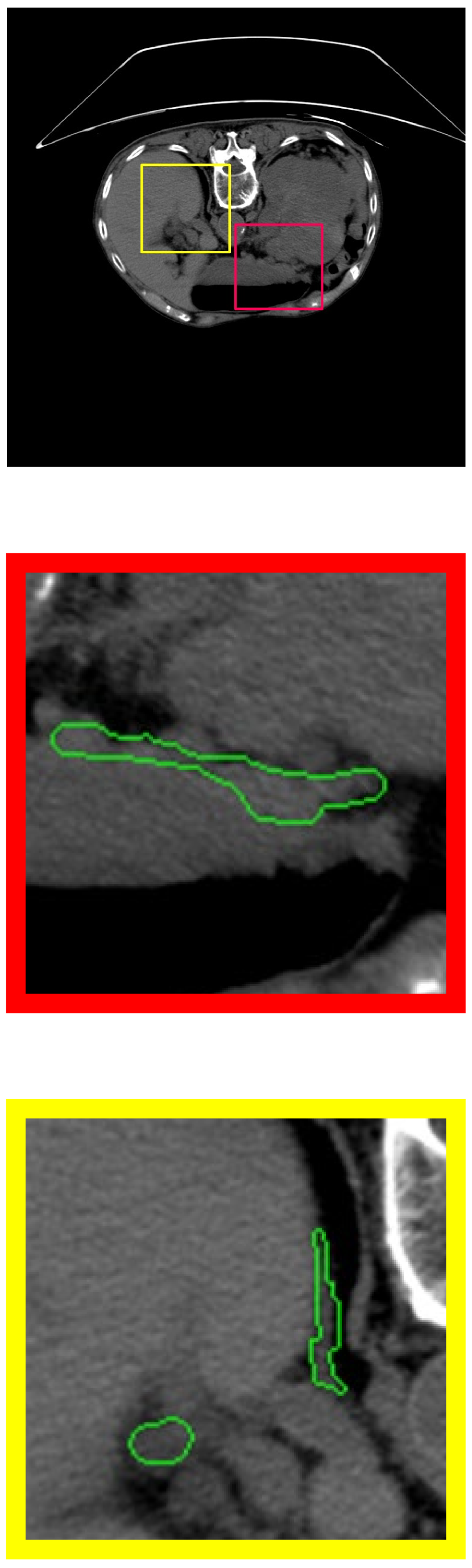
(a) Image

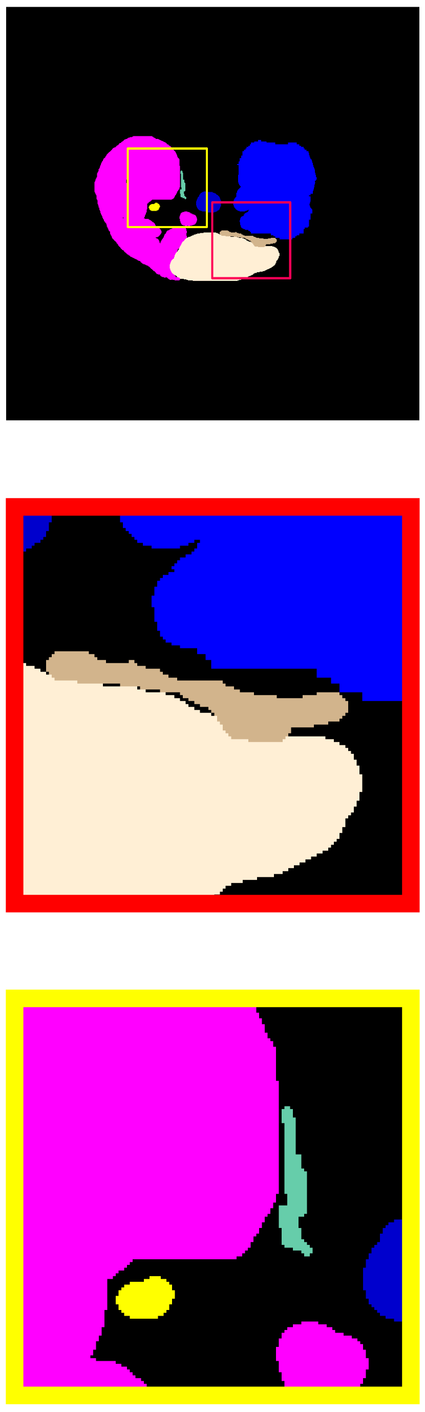
(b) Label

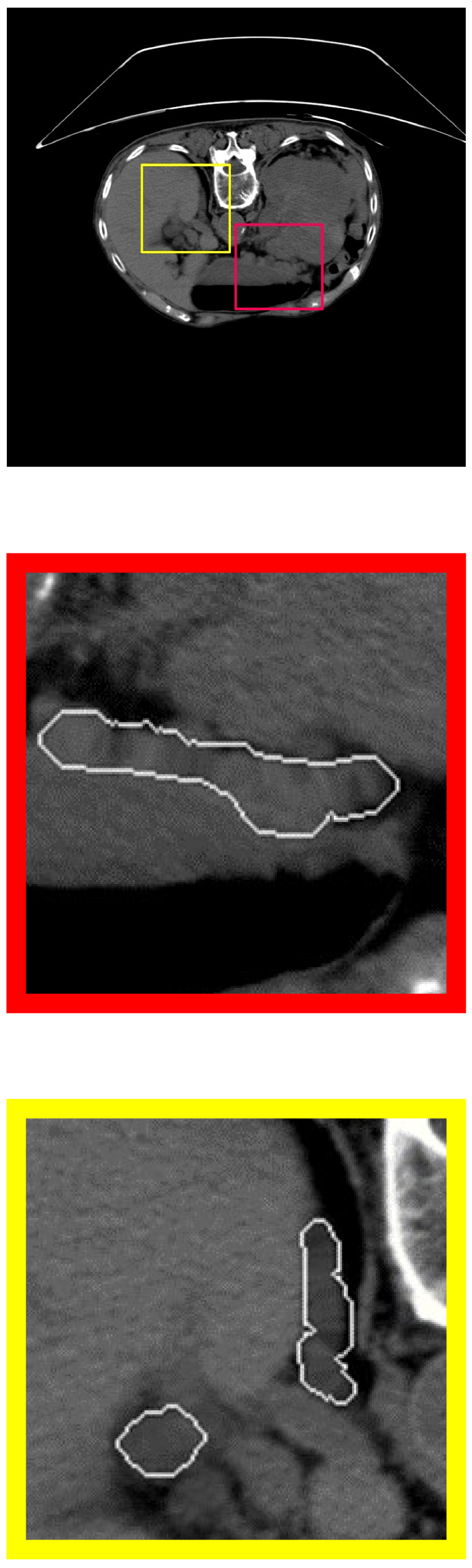
(c) Transformed Image

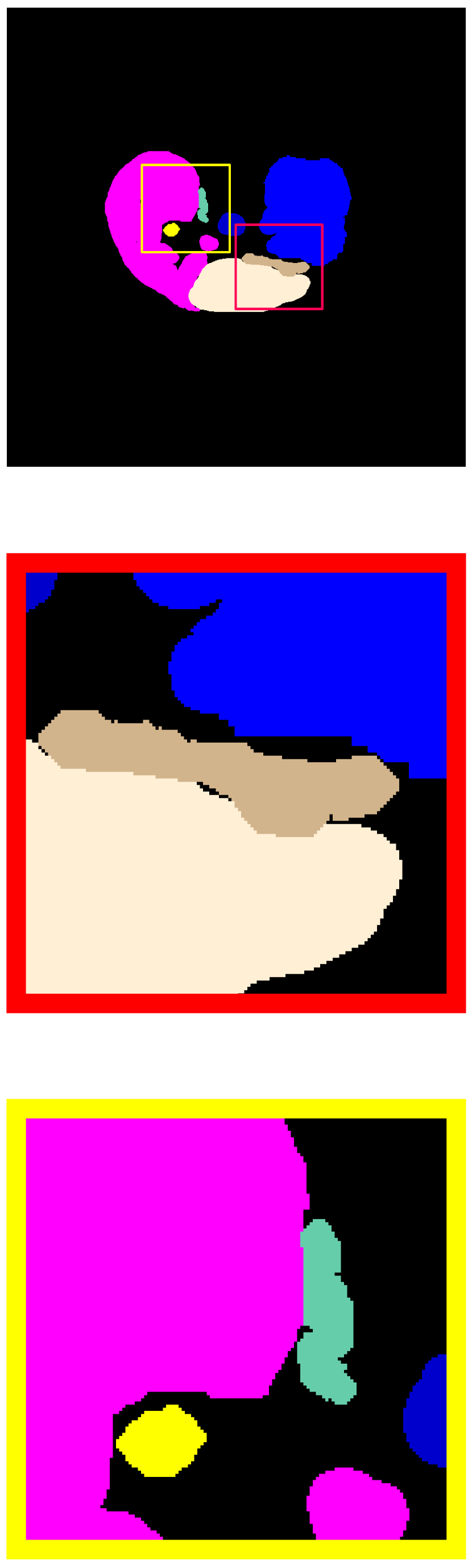
(d) Transformed Label

Figure 1: Motivation of STAC: enlarging smaller organs helps to alleviate imbalanced class distribution across different organs. The second and third rows are magnified images of the corresponding color boxes in the first row. The green curve in the Image represents the corresponding edges of the ground truth for categories with smaller pixel proportions. The white curve in the Transformed Image represents the edges of the corresponding ground-truth category, after processing with STAC.

The size of human organs can vary considerably, frequently causing a notable imbalance in the number of voxels among different categories (as shown in Fig. 1). Recently, some works address this issue of imbalanced class distribution in semi-supervised medical image segmentation by improving the network’s representation ability of imbalanced classes and refining their pseudo labels. For instance, Basak et al. [14] propose a dynamic learning strategy that tracks class-wise confidence during training and incorporates fuzzy fusion and robust class-wise sampling to improve segmentation performance for under-represented classes. To address the issue that the proposed model in [14] can not well model the difficulty, DHC [15] introduces Distribution-aware Debiased Weighting and Difficulty-aware Debiased Weighting, two strategies that use pseudo labels to dynamically address data and learning biases. Yuan et al. [16] combine a traditional linear-based classifier with a prototype-based classifier to alleviate the class-wise bias exhibited in each individual sample. However, these methods do not address the imbalanced class issue from an intuitive perspective in data level, that is, some organs are too small, resulting in low number of voxels.

In this paper, we enlarge smaller organs to alleviate the issue of imbalanced class distribution across different organs. In active contour methods, the contours evolve in the direction of the normal vector and are represented implicitly by a level set function to ensure stability during the evolution process. Inspired by this, we propose the Shape Transformation driven by Active Contour (STAC) method. STAC method utilizes a signed distance function (SDF) as the level set function to subtly represent the shapes of organs. It adjusts the voxels towards the direction of the steepest descent in SDF, which corresponds to the normal vector of the shape in zero level set. To ensure that voxels distant from the expanding organs remain unaffected, we develop a weight function based on SDF to carefully regulate the extent of deformation for each voxel. As shown in Fig. 1, we generate pairs of images and annotations (pseudo-labels for unlabeled images) that alleviate the class imbalance issue through our STAC method. Owing to the fact that evolution along the direction of the normal vector is less likely to produce distorted shapes, STAC can generate stable shape transformations, making the generated image more realistic. Using STAC for data-augmentation during training enhances the network’s ability to represent categories that have a smaller number of voxels. Experimental results demonstrate that enlarging smaller organs to alleviate the issue of imbalanced class distribution is effective. Our experiments demonstrate that the proposed STAC method significantly outperforms some state-of-the-art methods on two datasets.

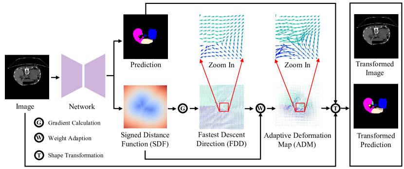
Figure 2: The pipeline of the proposed STAC framework, that is used for data-augmentation. For unlabeled samples, the Fastest Descent Direction (FDD) is defined as the gradient of the Signed Distance Function (SDF), which represents the direction of Adaptive Deformation Map (ADM). The degree of the ADM is SDF-based weight function. The shape transformation for enlarging smaller organs is obtained by interpolating the unlabeled images and pseudo labels according to the ADM. For labeled samples, the ADM is directly obtained using the label.

II Related Works

II-A Semi-supervised medical image segmentation

Semi-supervised learning (SSL) utilizes limited annotated data alongside abundant unlabeled data to enhance model performance. SSL methods are mainly categorized into self-training [17], where pseudo labels are assigned to unlabeled data for retraining, and consistency regularization [18, 8], which relies on the assumption that model outputs should remain stable under some perturbations [1]. Image-level perturbations include simple random augmentations [2] and adversarial approaches [5], while model-level perturbations involve direct stochastic modifications (e.g., Gaussian noise [6] or dropout [7]), parameter ensembling via exponential moving averages [8], or generating variations through different decoders or architectures [9, 10].

Semi-supervised learning is extensively employed in medical image segmentation, to ease the challenges of manual annotation. Consistency regularization methods [19, 20, 21, 22, 14, 23, 12] have significantly enhanced semi-supervised medical semantic segmentation, utilizing strategies such as the Mean Teacher framework [8] or Co-training [10] to introduce model-level variations. Another way involves creating diverse versions of the same image to enforce prediction consistency across image variations [24, 25, 26, 27, 28]. A prevalent method for image variations is the weak-to-strong paradigm [26], which utilizes images ranging from weakly to strongly augmented to promote model consistency. Several methods utilize adversarial training strategies to create adversarial perturbations on images, thereby enhancing the robustness of predictions against these perturbations [27, 28]. Additionally, an increasing number of techniques improve model performance by employing pseudo labels for training unlabeled images [12, 13]. The presence of noisy labels in pseudo labels for unlabeled images necessitates a careful assessment of their confidence levels [13, 29]. Additionally, certain methodologies emphasize the rectification of pseudo labels during the training process [30]. Beyond these strategies, other methods harness contrastive learning to attain consistent feature representation [3, 19].

II-B Class-Imbalanced Learning

Real-world datasets often exhibit a class-imbalanced label distribution, complicating the standard training and generalization of machine learning models [31]. Numerous algorithms [32, 33, 34, 35] have been proposed to address this problem. The most prevalent approach for addressing class imbalances involves rebalancing the training objective based on class-specific sample sizes. These methods are mainly categorized into re-weighting [32, 33], which impacts the loss function by assigning higher costs to examples from minority classes, and re-sampling [34, 35], which directly adjusts the label distribution by over-sampling the minority class or under-sampling the majority class, or both, to achieve a balanced sampling distribution.

The issue of class imbalance poses a significant challenge for extending existing SSL-based methods t o more practical settings. CReST [36] employs a self-training approach that enhances the SSL model by adaptively selecting pseudo-labeled data from the unlabeled set to augment the original labeled set. Unlike traditional self-training methods, CReST [36] chooses pseudo-labels based on label frequency to progressively balance the class distribution, favoring predictions from minority classes. Lin et al. [37] introduce the CLD method, which mitigates data bias by adjusting the overall loss function according to the voxel count of each class. Basak et al. [14] propose a dynamic learning strategy that monitors class-specific confidence throughout training, integrating fuzzy fusion and robust class-wise sampling to enhance segmentation performance for underrepresented classes. However, the model proposed in [14] does not consider the varying difficulty levels in modeling different categories. To address this issue, DHC [15] introduces two innovative strategies: Distribution-aware Debiased Weighting and Difficulty-aware Debiased Weighting. These approaches utilize pseudo labels to dynamically counteract data and learning biases.

III Method

III-A Curve Evolution Theory of Active Contour Model

A shape can be represented by its edge curves. Let $C:s\in[0,1]\rightarrow(x(s),y(s))\in\mathbb{R}^{2}$ denote a parametric curve. The outward normal of $C$ is $\vec{N}(s)=(y^{\prime}(s),-x^{\prime}(s))$. Many active contour methods [38, 39] evolve curves according to a velocity vector in the direction of its normal, which is expressed as $\frac{\partial C(x(s),y(s),t)}{\partial t}=V\vec{N}$. Level set method provides an effective and stable numerical solution for solving the above partial differential equation problem. In the level set implementation, an active curve $C$ is implicitly represented as the zero level set of a function $\phi$, denoted as $C=\{(x,y)|\phi(x,y)=0\}$. The evolution of the level set function is $\frac{\partial\phi(x,y,t)}{\partial t}=V||\nabla\phi||$.

Inspired by the evolution of curves along the normal vector and the level set representation, we design STAC to alleviate imbalanced class distribution. The pipeline of the proposed STAC is depicted in Fig. 2.

III-B Shape Transformation Driven by Active Contour Evolution

Let $\mathcal{D}=\mathcal{D}_{l}\cup\mathcal{D}_{u}$ be the whole training dataset, where $\mathcal{D}_{l}$ and $\mathcal{D}_{u}$ represent labeled and unlabeled dataset. For a labeled data pair $(X_{l},Y)\in\mathcal{D}_{l}$, we denote the minority classes as $M$. The organs we need to enlarge are $\mathcal{O}=\{(x,y,z)\in\mathbb{R}^{3}\;|\;Y(x,y,z)\in M\}$. We define the signed distance function as the level set representation of $\mathcal{O}$:

$$\phi_{\mathcal{O}}(\textbf{p})=\left\{\begin{aligned} &-\inf_{\textbf{q}\in\partial\mathcal{O}}\|\textbf{p}-\textbf{q}\|_{2},&\textbf{p}\in&\mathcal{O}_{\mathrm{in}}\\ &0,&\textbf{p}\in&\mathcal{\partial\mathcal{O}}\\ &+\inf_{\textbf{q}\in\partial\mathcal{O}}\|\textbf{p}-\textbf{q}\|_{2},&\textbf{p}\in&\mathcal{O}_{\mathrm{out}}\end{aligned}\right.$$ (1)

where $\partial\mathcal{O}$ represents the surface of $\mathcal{O}$. $\mathcal{O}_{\mathrm{in}}$ and $\mathcal{O}_{\mathrm{out}}$ denote the inside region and outside region of $\mathcal{O}$. The normal of $\phi_{\mathcal{O}}$ is denoted as $\vec{N}_{\mathcal{O}}(x,y,z)=(\frac{\partial\phi_{\mathcal{O}}}{\partial x},\frac{\partial\phi_{\mathcal{O}}}{\partial y},\frac{\partial\phi_{\mathcal{O}}}{\partial z})$. To ensure that voxels far from the expanding organs remain unaffected, we devise a weight coefficient $W_{\mathcal{O}}(x,y,z)$ based on SDF to carefully control the degree of deformation for each voxel.

$$W_{\mathcal{O}}(x,y,z)=\alpha\times e^{\beta\times\lvert\phi_{\mathcal{O}}(x,y,z)\rvert},$$ (2)

where $\alpha$ and $\beta$ are hyper-parameters. The adaptive deformation map $\vec{D}_{\mathcal{O}}(x,y,z)$ is obtained by multiplying the normal vector with a weight coefficient.

$$\vec{D}_{\mathcal{O}}(x,y,z)=W_{\mathcal{O}}(x,y,z)\times\vec{N}_{\mathcal{O}}(x,y,z).$$ (3)

By transforming the shape of the organs along the direction of the normal vector of the level set function, $X^{transformed}_{l}$ is denoted as:

$$X^{transformed}_{l}(x,y,z)=X_{l}(x +\frac{\partial\phi_{\mathcal{O}}}{\partial x}\times W_{\mathcal{O}},$$ (4)

$$y +\frac{\partial\phi_{\mathcal{O}}}{\partial y}\times W_{\mathcal{O}},$$

$$z +\frac{\partial\phi_{\mathcal{O}}}{\partial z}\times W_{\mathcal{O}}).$$

The same transformation is applied to generate $Y^{transformed}$.

$$Y^{transformed}(x,y,z)=Y(x +\frac{\partial\phi_{\mathcal{O}}}{\partial x}\times W_{\mathcal{O}},$$ (5)

$$y +\frac{\partial\phi_{\mathcal{O}}}{\partial y}\times W_{\mathcal{O}},$$

$$z +\frac{\partial\phi_{\mathcal{O}}}{\partial z}\times W_{\mathcal{O}}).$$

For unlabeled image $X_{u}\in D_{u}$, pseudo SDF $\phi_{pre}$ is predicted by the network. We use $\phi_{pre}$ to calculate the $\vec{D}_{pre}(x,y,z)$ as adaptive deformation map. $X_{u}$ and its pseudo-label $\hat{Y}$ is transformed using $\vec{D}_{pre}(x,y,z)$.

III-C Network architecture and training process

Our method can be integrated into any existing semi-supervised method, in a plug-and-play manner. In this paper, we use mutual supervision of two networks trained with cross-entropy loss (Refer to Eq.(6) and (8) below for this classic approach.), as an illustration of our proposal. For $i\in[1,2]$, let the feature extraction module be denoted as $f^{i}$ the classification head as $h^{i}$, as used in the base approach). We introduce an additional regression head for predicting the signed distance function, denoted as $g^{i}$. For labeled data pair as $(X_{l},Y)\in\mathcal{D}_{l}$, the supervised loss for segmentation task and regression task are:

$$\mathcal{L}_{seg}^{l} =\ell_{ce}({P}_{l}^{1},{Y})+\ell_{ce}({P}_{l}^{2},{Y}),$$ (6)

$$\mathcal{L}_{sdf}^{l} =||\phi_{pre}^{1}-\phi_{Y}||^{2}+||\phi_{pre}^{2}-\phi_{Y}||^{2}$$ (7)

where $\ell_{ce}$ is the cross-entropy loss, $P^{i}_{l}=f^{i}(h^{i}(X_{l}))$ is the output of the segmentation head, $\phi^{i}_{pre}=g^{i}(h^{i}(X_{l}))$ is the output of the level set prediction head, and superscript $i\in[1,2]$ means different network. In other words, we complement the basic supervised loss given in Eq. (6), with a specific loss $\mathcal{L}_{sdf}^{l}$, given in (7), dedicated to the signed distance function.

For unlabeled data $X_{u}\in D_{u}$, we denote the mutual supervision loss as:

$$\mathcal{L}_{seg}^{u} =\ell_{ce}({P}_{u}^{1},\hat{Y}^{2})+\ell_{dc}({P}_{u}^{2},\hat{Y}^{1}),$$ (8)

$$\mathcal{L}_{sdf}^{u} =||\phi_{pre}^{1}-\phi_{pre}^{2}||^{2}$$ (9)

where $\hat{Y}^{1}$ and $\hat{Y}^{2}$ are pseudo labels obtained from $P_{u}^{1}$ and $P_{u}^{2}$, respectively. Again, we complement the base loss for unlabeled data, given in Eq. (8), with a specific cost, given in Eq. (9) dedicated to the signed distance function.

TABLE I: Quantitative comparison of Dice score ($\uparrow$) between our proposed STAC and some class imbalance SSL segmentation methods on 2% labeled AMOS dataset.

Methods	Avg. Dice	Sp	RK	LK	Ga	Es	Li	St	Ao	IVC	PA	RAG	LAG	Du	Bl	P/U
V-Net (fully)	76.5	92.2	92.2	93.3	65.5	70.3	95.3	82.4	91.4	85.0	74.9	58.6	58.1	65.6	64.4	58.3
CReST [36]	32.1	44.6	45.6	49.4	18.3	18.3	52.5	35.9	35.9	42.5	25.4	19.1	10.5	24.4	37.0	22.2
CReST+STAC	37.1(+5.0)	63.5	58.5	55.5	32.6	22.1	69.2	24.3	49.1	48.1	18.6	22.6	13.1	21.8	32.9	25.6
SimiS [40]	37.5	62.4	60.4	59.5	29.7	0.0	70.2	37.1	50.0	46.2	27.8	21.5	8.1	21.0	43.1	26.3
SimiS+STAC	38.0(+0.5)	59.6	59.9	58.9	29.5	0.0	67.9	39.6	52.7	50.6	29.6	19.4	4.9	26.5	45.9	25.6
CLD [37]	36.6	60.9	54.1	56.4	28.1	0.0	67.7	35.6	48.1	48.7	29.7	28.0	6.8	22.1	40.5	22.4
CLD+STAC	40.0(+3.4)	63.2	61.4	59.4	32.4	0.0	73.2	39.7	59.3	56.2	37.0	19.1	8.1	19.4	46.4	25.1
DHC [15]	37.6	62.3	60.1	59.7	27.7	18.3	69.2	31.6	50.9	42.7	24.4	23.9	9.5	13.5	46.7	23.7
DHC+STAC	45.8(+8.2)	63.2	63.6	62.8	38.4	27.3	73.5	45.2	66.5	57.3	41.5	29.9	13.7	31.8	45.6	27.1

TABLE II: Quantitative comparison of Dice score ($\uparrow$) between our proposed STAC and some class imbalance SSL segmentation methods on 5% labeled AMOS dataset.

Methods	Avg. Dice	Sp	RK	LK	Ga	Es	Li	St	Ao	IVC	PA	RAG	LAG	Du	Bl	P/U
V-Net (fully)	76.5	92.2	92.2	93.3	65.5	70.3	95.3	82.4	91.4	85.0	74.9	58.6	58.1	65.6	64.4	58.3
CReST [36]	47.0	74.1	66.7	67.6	24.1	32.3	86.1	47.6	72.4	54.6	39.5	25.8	13.4	29.2	44.6	27.3
CReST+STAC	48.0(+1.0)	73.6	71.1	70.2	31.2	32.3	86.0	44.0	66.9	57.5	40.0	24.2	18.3	29.7	46.9	28.2
SimiS [40]	49.6	80.1	72.7	69.5	36.8	34.9	88.1	53.4	78.5	58.3	43.0	29.3	12.4	21.9	45.9	19.6
SimiS+STAC	53.7(+4.1)	79.0	77.4	74.0	41.0	44.7	88.3	55.2	78.8	59.2	37.5	33.5	28.3	32.2	48.0	29.5
CLD [37]	49.3	80.2	77.6	71.4	34.8	36.5	88.5	44.0	78.7	57.9	44.3	30.1	17.0	23.6	43.4	12.9
CLD+STAC	50.9(+1.6)	81.1	75.6	75.9	39.9	40.4	88.2	51.4	78.8	61.5	47.8	28.9	17.5	31.8	45.9	0.2
DHC [15]	49.2	80.6	68.3	70.6	34.1	35.1	85.3	51.9	73.4	59.0	48.0	26.3	16.0	27.3	42.9	20.7
DHC+STAC	53.9(+4.7)	79.9	78.0	76.3	38.5	45.9	85.8	53.6	76.4	62.0	47.3	32.1	27.1	38.1	47.8	20.0

TABLE III: Quantitative comparison of average surface distance (ASD $\downarrow$) between our proposed STAC and some class imbalance SSL segmentation methods.

Methods	Amos		Synapse
	2%	5%	10%	20%
CReST [36]	22.5	9.7	50.9	29.6
CReST + STAC	19.3	5.9	31.0	14.3
SimiS [40]	26.3	10.9	32.9	38.4
SimiS + STAC	26.2	5.6	31.9	32.7
CLD [37]	28.6	11.4	37.9	20.2
CLD + STAC	26.0	13.6	22.8	17.1
DHC [15]	20.1	11.2	25.8	9.8
DHC + STAC	13.5	6.4	26.7	8.9

TABLE IV: Quantitative results of the proposed STAC compared with other shape transformation on AMOS dataset using 2% labeled images under the DHC [15] baseline.

	DHC [15]	+Elastic	+Anatomy [41]	+STAC
Dice (%)	37.6	40.1	40.0	45.8
ASD	20.1	20.7	16.6	13.5

TABLE V: Quantitative results of applying STAC on labeled images (L) and unlabeled images (U) on AMOS dataset using 2% labeled images under the DHC [15] baseline.

	DHC [15]	+STAC (L)	+STAC (U+L)
Dice (%)	37.6	41.7	45.8
ASD	20.1	17.1	13.5

TABLE VI: Quantitative comparison of Dice score ($\uparrow$) between our proposed STAC and some class imbalance SSL segmentation methods on 10% labeled Synapse dataset.

Methods	Avg. Dice	Sp	RK	LK	Ga	Es	Li	St	Ao	IVC	PSV	PA	RAG	LAG
V-Net (fully)	62.0	84.6	77.2	73.8	73.3	38.2	94.6	68.4	72.1	71.2	58.2	48.5	17.9	29.0
CReST [36]	24.3	39.6	44.7	26.3	26.3	1.4	59.3	16.2	38.5	30.2	3.7	8.1	20.1	1.9
CReST+STAC	26.9(+2.6)	46.9	49.3	36.5	30.2	9.6	51.5	27.4	42.5	23.0	2.9	3.7	23.5	3.8
SimiS [40]	24.5	43.1	38.0	43.8	16.5	4.5	68.1	21.8	46.3	14.4	4.7	7.6	0.5	9.5
SimiS+STAC	29.1(+4.6)	48.1	43.8	42.4	18.3	9.1	54.1	23.7	59.6	50.9	1.6	11.6	2.0	14.0
CLD [37]	24.1	48.1	45.9	39.1	1.0	9.4	46.8	19.4	52.6	33.3	8.2	2.4	5.3	1.9
CLD+STAC	29.7(+5.6)	53.1	55.0	45.8	0.4	9.7	54.1	35.7	50.0	49.2	8.1	10.4	0.6	14.6
DHC  [15]	30.0	60.7	43.9	42.4	0.0	19.2	61.2	36.9	48.8	38.3	9.0	11.8	13.2	4.9
DHC+STAC	34.8(+4.8)	61.4	61.5	60.3	0.2	13.9	74.3	35.1	61.0	53.1	11.6	10.7	9.5	0.0

TABLE VII: Quantitative comparison of Dice score ($\uparrow$) between our proposed STAC and some class imbalance SSL segmentation methods on 20% labeled Synapse dataset.

Methods	Avg. Dice	Sp	RK	LK	Ga	Es	Li	St	Ao	IVC	PSV	PA	RAG	LAG
V-Net (fully)	62.0	84.6	77.2	73.8	73.3	38.2	94.6	68.4	72.1	71.2	58.2	48.5	17.9	29.0
CReST [36]	36.5	68.5	66.7	53.1	36.9	3.0	83.5	25.7	40.6	39.8	9.0	15.8	14.3	17.6
CReST+STAC	38.4 (+1.9)	62.3	70.5	58.8	27.0	19.4	76.0	33.8	52.7	37.8	2.3	15.5	17.2	26.1
SimiS [40]	41.8	84.6	78.5	74.7	2.9	0.0	82.5	44.0	66.3	64.2	29.1	17.7	0.0	0.0
SimiS+STAC	43.5 (+1.7)	83.6	77.4	76.2	4.3	0.0	81.2	43.2	74.5	68.4	30.0	23.6	3.7	0.0
CLD [37]	45.0	76.6	76.9	72.3	9.9	0.0	87.4	34.1	63.3	64.7	14.5	19.4	29.1	37.7
CLD+STAC	46.2 (+1.2)	82.9	79.4	79.4	17.4	0.0	87.5	19.1	72.3	61.4	20.0	24.4	27.9	29.7
DHC  [15]	47.8	75.5	73.3	77.0	1.7	24.5	80.8	38.8	65.6	57.2	28.4	20.6	25.7	52.2
DHC+STAC	50.7 (+2.9)	84.2	81.4	80.4	6.5	26.3	84.8	33.2	76.4	65.8	38.3	21.9	22.8	38.0

In summary, our proposal boils down to adding to a base network, another head to predict the signed distance function, together with a specific cost function for training this head. During the training process, we use $X^{transformed}$ (Eq. (4)) and $Y^{transformed}$ (Eq. (5)) as data-augmentation (see Fig. 2).

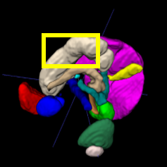
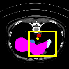
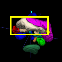
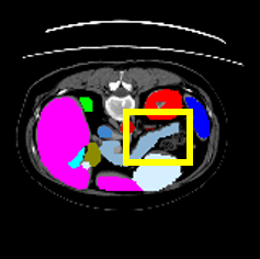
(a) GT

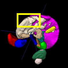
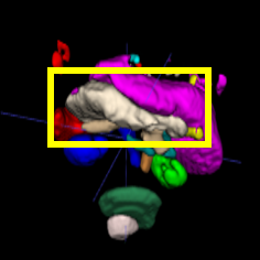
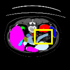
(b) DHC+STAC

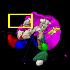
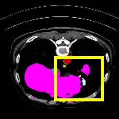
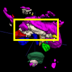
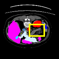
(c) DHC

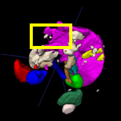
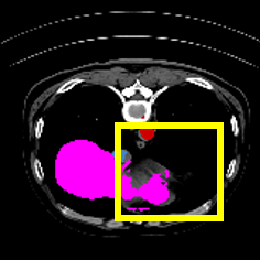
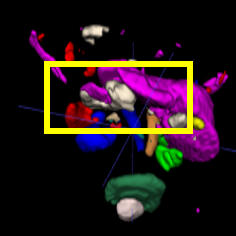
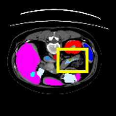
(d) CLD

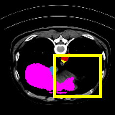
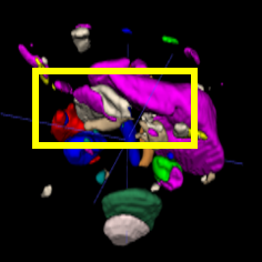
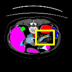
(e) CReST

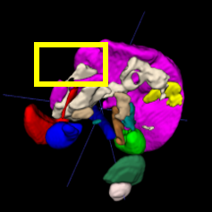
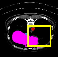
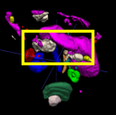
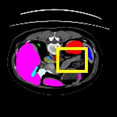
(f) SimiS

Figure 3: Some qualitative segmentation results of STAC and some other methods on AMOS dataset. The first and third rows are 3D views, and the second and fourth rows are 2D slices.

IV Experiments

IV-A Dataset and Implementation Details.

To address class imbalance in semi-supervised medical image segmentation, we adhere to the experimental setup proposed in DHC [15]. We use two different benchmarks: the Synapse [42] and AMOS [43] datasets. The AMOS dataset consists of 360 scans, which are divided into 216, 24 and 120 scans for training, validation, and testing, covering 15 foreground classes, including spleen (Sp), right kidney (RK), left kidney (LK), gallbladder (Ga), esophagus (Es), liver (Li), stomach (St), aorta (Ao), inferior vena cava (IVC), pancreas (PA), right adrenal gland (RAG), left adrenal gland (LAG), duodenum (Du), bladder (Bl), prostate/uterus (P/U). Compared with AMOS, Synapse excludes Du, Bl and P/U but adds portal & splenic veins (PSV). Synapse dataset consists of 30 scans, and we follow DHC [15] splitting them as 20, 4 and 6 scans for training, validation, and testing, respectively. The proposed method is evaluated with two widely used metrics in semi-supervised medical image segmentation: Dice coefficient (Dice) and the average surface distance (ASD).

IV-B Comparison with State-of-the-Art Methods.

To validate the effectiveness of our proposed Shape Transformation driven by Active Contour (STAC) method, we conduct experimental evaluations by integrating STAC with four established baselines: CReST [36], SimiS [40], CLD [37], and DHC [15], which address the class imbalance problem. Following the experiments setting in DHC [15], we conduct semi-supervised experiments on the AMOS dataset using 2% and 5% of the labeled data, and experiments on the Synapse dataset using 10% and 20% of the labeled data. The results of the AMOS dataset [43] experiments are depicted in Tab. I (2%) and Tab. II (5%), and the results of the Synapse dataset [42] experiments are presented in Tab. VI (10%) and Tab. VII (20%). Under the setting of using 2% labeled data of AMOS dataset [43], applying our STAC to the state-of-the-art DHC [15] method resulted in a 8.2% improvement in the Dice coefficient. In the scenario where 5% of the AMOS dataset is labeled, the implementation of our STAC on DHC [15] led to an enhancement of 4.7% in the Dice coefficient. On the Synapse dataset [42], when using 10% labeled data, applying our method to the four approaches—CReST [36] , SimiS [40], CLD [37], and DHC [15]—results in Dice coefficient improvements of 2.6%, 4.6%, 5.6%, and 4.8%, respectively. Some qualitative results are shown in Fig. 3.

IV-C Ablation Studies.

Ablation study using other shape transformation. While random elastic [44] is a simple shape transformation augmentation, it cannot be used to enlarge organs. Tab. IV shows that, while random elastic marginally enhances the Dice coefficient, it increases ASD by altering organ contours. STAC, by evolving along the normal vector to avoid distorted shapes, produces more realistic and stable shape transformations. This leads to a 5.8% improvement in Dice scores over the anatomy-informed shape transformation method [41].

Ablation study on hyperparameters ($\alpha$ and $\beta$) of $W_{\mathcal{O}}$. The proposed STAC only include $\alpha$ and $\beta$ as hyperparameters. The curve of the SDF-based weight function with different parameters $\alpha$ and $\beta$ is shown in Fig. 4. The experimental results obtained by controlling the degree of shape change using the SDF-based weight function are shown in Fig. 5. The best results are achieved when $\alpha=1$ and $\beta=-1$, with a Dice score of 53.9.

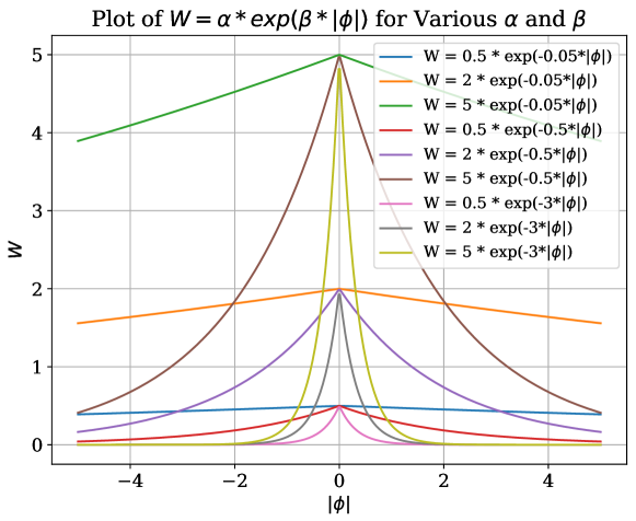
Figure 4: Plot of the SDF-based weight function with different parameters $\alpha$ and $\beta$.

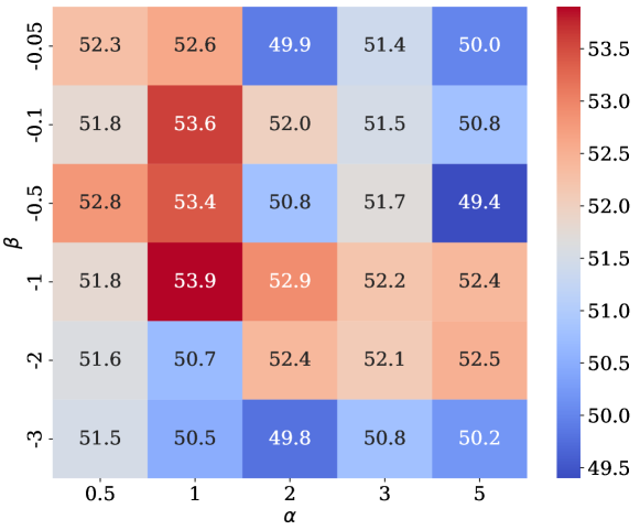
Figure 5: Dice score of using different values for parameters $\alpha$ and $\beta$ on AMOS dataset using 5% labeled images under the DHC [15] baseline. The numerical values in the heatmap represent Dice scores.

Ablation study focusing on the application of shape transformation exclusively to labeled data. Our method can be applied solely to the images and annotation pairs of labeled samples, which does not alter the training process. As shown in Tab. V, performing shape transformations only on labeled samples also significantly improves the results.

V Conclusion

This paper introduces a novel Shape Transformation driven by Active Contour (STAC) method for addressing the issue of imbalanced class distribution in 3D medical image segmentation. By utilizing the Signed Distance Function (SDF) as the level set function, and deforming the voxels in the direction of the steepest descent of SDF, STAC effectively enlarges smaller organs, balancing the class distribution across various organs. This approach ensures that voxels distant from the expanding organs remain unchanged by designing an SDF-based weight function to control the degree of deformation. Experimental results show that using STAC as a data-augmentation process in four baseline models yields consistent and significant improvements, demonstrating the effectiveness of our method.

VI Acknowledgement

This work was supported in part by the National Key Research and Development Program of China (2023YFC2705700), NSFC 62222112 and 62176186, the NSF of Hubei Province of China (2024AFB245).

References

- [1] Y. Chen, M. Mancini, X. Zhu, and Z. Akata, “Semi-supervised and unsupervised deep visual learning: A survey,” IEEE Trans. on Pattern Anal. and Mach. Intell., 2022.
- [2] M. Sajjadi, M. Javanmardi, and T. Tasdizen, “Regularization with stochastic transformations and perturbations for deep semi-supervised learning,” Proc. of Advances in Neural Information Processing Systems, vol. 29, 2016.
- [3] C. You, Y. Zhou, R. Zhao, L. Staib, and J. S. Duncan, “SimCVD: Simple contrastive voxel-wise representation distillation for semi-supervised medical image segmentation,” IEEE Trans. on Medical Imaging, vol. 41, no. 9, pp. 2228–2237, 2022.
- [4] T. Suzuki and I. Sato, “Adversarial transformations for semi-supervised learning,” in Proc. of the AAAI Conf. on Artificial Intelligence, vol. 34, 2020, pp. 5916–5923.
- [5] T. Miyato, S.-i. Maeda, M. Koyama, and S. Ishii, “Virtual adversarial training: a regularization method for supervised and semi-supervised learning,” IEEE Trans. on Pattern Anal. and Mach. Intell., vol. 41, no. 8, pp. 1979–1993, 2018.
- [6] A. Rasmus, M. Berglund, M. Honkala, H. Valpola, and T. Raiko, “Semi-supervised learning with ladder networks,” Proc. of Advances in Neural Information Processing Systems, vol. 28, 2015.
- [7] S. Park, J. Park, S.-J. Shin, and I.-C. Moon, “Adversarial dropout for supervised and semi-supervised learning,” in Proc. of the AAAI Conf. on Artificial Intelligence, vol. 32, 2018.
- [8] A. Tarvainen and H. Valpola, “Mean teachers are better role models: Weight-averaged consistency targets improve semi-supervised deep learning results,” Advances in neural information processing systems, vol. 30, 2017.
- [9] Y. Wu, Z. Ge, D. Zhang, M. Xu, L. Zhang, Y. Xia, and J. Cai, “Mutual consistency learning for semi-supervised medical image segmentation,” Medical Image Analysis, vol. 81, p. 102530, 2022.
- [10] S. Qiao, W. Shen, Z. Zhang, B. Wang, and A. Yuille, “Deep co-training for semi-supervised image recognition,” in Proc. of European Conf. on Computer Vision, 2018, pp. 135–152.
- [11] X. Chen, Y. Yuan, G. Zeng, and J. Wang, “Semi-supervised semantic segmentation with cross pseudo supervision,” in Proc. of IEEE Conf. on Computer Vision and Pattern Recognition, 2021, pp. 2613–2622.
- [12] F. Lyu, M. Ye, J. F. Carlsen, K. Erleben, S. Darkner, and P. C. Yuen, “Pseudo-label guided image synthesis for semi-supervised covid-19 pneumonia infection segmentation,” IEEE Trans. on Medical Imaging, vol. 42, no. 3, pp. 797–809, 2022.
- [13] P. Qiao, H. Li, G. Song, H. Han, Z. Gao, Y. Tian, Y. Liang, X. Li, S. K. Zhou, and J. Chen, “Semi-supervised ct lesion segmentation using uncertainty-based data pairing and swapmix,” IEEE Trans. on Medical Imaging, 2022.
- [14] H. Basak, S. Ghosal, and R. Sarkar, “Addressing class imbalance in semi-supervised image segmentation: A study on cardiac mri,” in Proc. of Intl. Conf. on Medical Image Computing and Computer Assisted Intervention, 2022, pp. 224–233.
- [15] H. Wang and X. Li, “Dhc: Dual-debiased heterogeneous co-training framework for class-imbalanced semi-supervised medical image segmentation,” in International Conference on Medical Image Computing and Computer-Assisted Intervention, 2023, pp. 582–591.
- [16] Y. Yuan, X. Wang, X. Yang, R. Li, and P.-A. Heng, “Semi-supervised class imbalanced deep learning for cardiac mri segmentation,” in Proc. of Intl. Conf. on Medical Image Computing and Computer Assisted Intervention, 2023, pp. 459–469.
- [17] Y. Grandvalet and Y. Bengio, “Semi-supervised learning by entropy minimization,” in Proc. of Advances in Neural Information Processing Systems, 2005.
- [18] S. Laine and T. Aila, “Temporal ensembling for semi-supervised learning,” in Proc. of International Conference on Learning Representations, 2016.
- [19] H. Basak and Z. Yin, “Pseudo-label guided contrastive learning for semi-supervised medical image segmentation,” in Proc. of IEEE Conf. on Computer Vision and Pattern Recognition, 2023, pp. 19 786–19 797.
- [20] T. Lei, D. Zhang, X. Du, X. Wang, Y. Wan, and A. K. Nandi, “Semi-supervised medical image segmentation using adversarial consistency learning and dynamic convolution network,” IEEE Trans. on Medical Imaging, 2022.
- [21] Q. Jin, H. Cui, C. Sun, J. Zheng, L. Wei, Z. Fang, Z. Meng, and R. Su, “Semi-supervised histological image segmentation via hierarchical consistency enforcement,” in Proc. of Intl. Conf. on Medical Image Computing and Computer Assisted Intervention, 2022, pp. 3–13.
- [22] J. Xiang, P. Qiu, and Y. Yang, “FUSSNet: Fusing two sources of uncertainty for semi-supervised medical image segmentation,” in Proc. of Intl. Conf. on Medical Image Computing and Computer Assisted Intervention, 2022, pp. 481–491.
- [23] Y. Wang, B. Xiao, X. Bi, W. Li, and X. Gao, “MCF: Mutual correction framework for semi-supervised medical image segmentation,” in Proc. of IEEE Conf. on Computer Vision and Pattern Recognition, 2023, pp. 15 651–15 660.
- [24] W. Huang, C. Chen, Z. Xiong, Y. Zhang, X. Chen, X. Sun, and F. Wu, “Semi-supervised neuron segmentation via reinforced consistency learning,” IEEE Trans. on Medical Imaging, vol. 41, no. 11, pp. 3016–3028, 2022.
- [25] X. Xu, T. Sanford, B. Turkbey, S. Xu, B. J. Wood, and P. Yan, “Shadow-consistent semi-supervised learning for prostate ultrasound segmentation,” IEEE Trans. on Medical Imaging, vol. 41, no. 6, pp. 1331–1345, 2021.
- [26] J. Fan, B. Gao, H. Jin, and L. Jiang, “Ucc: Uncertainty guided cross-head co-training for semi-supervised semantic segmentation,” in Proc. of IEEE Conf. on Computer Vision and Pattern Recognition, 2022, pp. 9947–9956.
- [27] H. Peiris, Z. Chen, G. Egan, and M. Harandi, “Duo-SegNet: adversarial dual-views for semi-supervised medical image segmentation,” in Proc. of Intl. Conf. on Medical Image Computing and Computer Assisted Intervention, 2021, pp. 428–438.
- [28] P. Wang, J. Peng, M. Pedersoli, Y. Zhou, C. Zhang, and C. Desrosiers, “CAT: Constrained adversarial training for anatomically-plausible semi-supervised segmentation,” IEEE Trans. on Medical Imaging, 2023.
- [29] G. Wang, S. Zhai, G. Lasio, B. Zhang, B. Yi, S. Chen, T. J. Macvittie, D. Metaxas, J. Zhou, and S. Zhang, “Semi-supervised segmentation of radiation-induced pulmonary fibrosis from lung ct scans with multi-scale guided dense attention,” IEEE Trans. on Medical Imaging, vol. 41, no. 3, pp. 531–542, 2021.
- [30] Y. Liu, Y. Tian, Y. Chen, F. Liu, V. Belagiannis, and G. Carneiro, “Perturbed and strict mean teachers for semi-supervised semantic segmentation,” in Proc. of IEEE Conf. on Computer Vision and Pattern Recognition, 2022, pp. 4258–4267.
- [31] Z. Liu, Z. Miao, X. Zhan, J. Wang, B. Gong, and S. X. Yu, “Large-scale long-tailed recognition in an open world,” in Proc. of IEEE Conf. on Computer Vision and Pattern Recognition, 2019, pp. 2537–2546.
- [32] K. Cao, C. Wei, A. Gaidon, N. Arechiga, and T. Ma, “Learning imbalanced datasets with label-distribution-aware margin loss,” Proc. of Advances in Neural Information Processing Systems, vol. 32, 2019.
- [33] J. Shu, Q. Xie, L. Yi, Q. Zhao, S. Zhou, Z. Xu, and D. Meng, “Meta-weight-net: Learning an explicit mapping for sample weighting,” Proc. of Advances in Neural Information Processing Systems, vol. 32, 2019.
- [34] J. Byrd and Z. Lipton, “What is the effect of importance weighting in deep learning?” in Proc. of Intl. Conf. on Machine Learning, 2019, pp. 872–881.
- [35] M. Buda, A. Maki, and M. A. Mazurowski, “A systematic study of the class imbalance problem in convolutional neural networks,” Neural networks, vol. 106, pp. 249–259, 2018.
- [36] C. Wei, K. Sohn, C. Mellina, A. Yuille, and F. Yang, “Crest: A class-rebalancing self-training framework for imbalanced semi-supervised learning,” in Proc. of IEEE Conf. on Computer Vision and Pattern Recognition, 2021, pp. 10 857–10 866.
- [37] Y. Lin, H. Yao, Z. Li, G. Zheng, and X. Li, “Calibrating label distribution for class-imbalanced barely-supervised knee segmentation,” in Proc. of Intl. Conf. on Medical Image Computing and Computer Assisted Intervention, 2022, pp. 109–118.
- [38] Z. Wang, D. Acuna, H. Ling, A. Kar, and S. Fidler, “Object instance annotation with deep extreme level set evolution,” in Proc. of IEEE Conf. on Computer Vision and Pattern Recognition, 2019, pp. 7500–7508.
- [39] C. Li, C. Xu, C. Gui, and M. D. Fox, “Distance regularized level set evolution and its application to image segmentation,” IEEE Trans. on Image Processing, vol. 19, no. 12, pp. 3243–3254, 2010.
- [40] H. Chen, Y. Fan, Y. Wang, J. Wang, B. Schiele, X. Xie, M. Savvides, and B. Raj, “An embarrassingly simple baseline for imbalanced semi-supervised learning,” arXiv preprint arXiv:2211.11086, 2022.
- [41] B. Kovacs, N. Netzer, M. Baumgartner, C. Eith, D. Bounias, C. Meinzer, P. F. Jäger, K. S. Zhang, R. Floca, A. Schrader et al., “Anatomy-informed data augmentation for enhanced prostate cancer detection,” in Proc. of Intl. Conf. on Medical Image Computing and Computer Assisted Intervention, 2023, pp. 531–540.
- [42] B. Landman, Z. Xu, J. E. Igelsias, M. Styner, T. Langerak, and A. Klein, “Miccai multi-atlas labeling beyond the cranial vault–workshop and challenge,” in Proc. MICCAI: Multi-Atlas Labeling Beyond Cranial Vault-Workshop Challenge, 2015.
- [43] Y. Ji, H. Bai, J. Yang, C. Ge, Y. Zhu, R. Zhang, Z. Li, L. Zhang, W. Ma, X. Wan et al., “Amos: A large-scale abdominal multi-organ benchmark for versatile medical image segmentation,” arXiv preprint arXiv:2206.08023, 2022.
- [44] S. Connor and T. M. Khoshgoftaar, “A survey on image data augmentation for deep learning,” Journal of big data, vol. 6, no. 1, pp. 1–48, 2019.