CUT-E as a expansion for multiscale molecular polariton dynamics
Abstract
Molecular polaritons arise when the collective coupling between an ensemble of molecules and an optical mode exceeds individual photon and molecular linewidths. The complexity of their description stems from their multiscale nature, where the local dynamics on each molecule can, in principle, be influenced by the collective behavior of the entire ensemble. To address this, we previously introduced a formalism called collective dynamics using truncated equations (CUT-E). CUT-E approaches the problem in two stages. First, it exploits permutational symmetries to obtain a substantial simplification of the problem. However, this is often insufficient for parameter regimes relevant to most experiments. Second, it takes the exact solution of the problem in the limit as a reference and derives systematic corrections. Here we provide a novel derivation of CUT-E based on recently developed bosonization techniques. We lay down its connections with expansions that are ubiquitous in other fields of physics, and present previously unexplored key aspects of this formalism, including various types of approximations and extensions to high excitation manifolds.
I Introduction
Strong light-matter coupling is achieved when the coherent energy exchange rate between the degrees of freedom (DOF) of matter and a confined electromagnetic field surpasses the losses from either component, forming hybrid light-matter states known as polaritons Ribeiro et al. (2018); Ebbesen, Rubio, and Scholes (2023); Xiong (2023); Bhuyan et al. (2023); Mandal et al. (2023); Xiang and Xiong (2024). In molecular systems, strong coupling is typically attained through the interaction of an ensemble of molecules with a microcavity mode due to the small magnitude of the transition dipole moment of individual molecules. Over the past decade, microcavities have garnered significant attention for their potential for enhanced energy and charge transport Coles et al. (2014); Reitz, Mineo, and Genes (2018); DelPo et al. (2021); Martínez-Martínez et al. (2018); Xiang et al. (2020); Koner et al. (2023); Peng and Rabani (2024), modification and control of chemical reactions Hutchison et al. (2012); Dunkelberger et al. (2016); Zeng et al. (2023); Dunkelberger et al. (2022); Nelson and Weichman (2024), and room-temperature polariton condensation Ishii et al. (2022); Kéna-Cohen and Forrest (2010), among other remarkable phenomena. However, many of these effects remain unresolved, largely due to the computational challenges posed by the multiscale nature of the systems in question. This theoretical complication arises as the collective behavior of the ensemble can influence the local dynamics of each molecule. As a result, most existing molecular polariton simulations are limited to a few tens of molecules using sophisticated numerical methods Luk et al. (2017); Groenhof et al. (2019); Li, Nitzan, and Subotnik (2022); Li and Hammes-Schiffer (2023) or single- or few-molecule systems using ab initio techniques Sidler et al. (2021, 2022); Schäfer (2022); El Moutaoukal et al. .
To address these challenges, we recently introduced a formalism called collective dynamics using truncated equations (CUT-E) Pérez-Sánchez et al. (2023). First, it exploits permutational symmetry for an efficient representation of the system. Second, it provides a simple solution to the problem for large by deriving an exact solution in the limit and subsequently carrying out systematic corrections. This resembles many other techniques in different areas of physics. Witten (1979); Hooft (1974); Chatterjee (1990); Witten (1980); Vollhardt (2012). One of the most seminal instances is the ’t Hooft’s large- expansion that simplifies the analysis of color group gauge theories, and established a duality between quantum chromodynamics (QCD) and string theory in the large- limit Hooft (1974). The use of this top-down approach to study molecular polaritons has recently grown in popularity Zeb, Kirton, and Keeling (2018a); Fowler-Wright, Lovett, and Keeling (2022); Cui and Nizan (2022); Zeb, Kirton, and Keeling (2022); Gu (2023); Sidler, Ruggenthaler, and Rubio (2024); Lindoy, Mandal, and Reichman (2024), as it brings substantial computational efficiency compared to the traditional bottom-up methodologies often applied to mesoscopic ensembles. Our original derivation of CUT-E was carried out in a pedestrian fashion using a first quantization approach to the many-molecule plus cavity wavefunction. Here, we provide a much simpler re-derivation using a recently developed bosonic mapping of polaritons and make new direct connections of CUT-E with expansions of other fields.
The article is organized as follows: in Section II, we present the Tavis-Cummings-Holstein Hamiltonian and establish a bosonic mapping to the vibronic modes of the single molecule. In section III, we state the difference between the collective vs single-molecule light-matter coupling regimes. In section IV, we rigorously solve the quantum dynamics in the first excitation manifold for the case of . Then, we show that exact quantities can be calculated for finite via a expansion. In section V, we present our method in a broader setting and connect it to expansions in other areas of physics. In section VI, we briefly comment on the open problems in the polaritonic quantum dynamics in high excitation manifolds. Sections II, III, and IV yield new insights and simpler re-derivations of results that have been already reported Pérez-Sánchez et al. (2023, 2024a); Yuen-Zhou and Koner (2024); Pérez-Sánchez and Yuen-Zhou (2024); Schwennicke et al. (2024), while sections V and VI contain entirely new results.
II Model
II.1 First-quantized picture
The Hamiltonian for an ensemble of non-interacting molecules strongly coupled to a confined optical mode of a microcavity can be written as
| (1) |
where is the molecular Hamiltonian of the th molecule, is the Hamiltonian for the cavity modes, and is the light-matter interaction between the th molecule and the cavity modes.
For simplicity, let us consider all molecules to be identical and the cavity to have a single photon mode. Although these assumptions are important for our method to work, we discuss how to generalize them to account for disorder and the multimode nature of the cavity further below. Also, for pedagogical purposes, let us assume the Born-Oppenheimer approximation for the molecular Hamiltonian and the Condon and rotating wave approximations to the light-matter interaction (these approximations can be easily relaxed). Thus, the molecular polariton Hamiltonian can be written as
| (2) |
where is the kinetic energy operator, are the ground/excited potential energy surfaces (PES), is the single-molecule light-matter coupling strength, and is the annihilation operator of a photon in the cavity mode.
Notice that is invariant under the permutation of any pair of molecules. For a permutationally-symmetric initial wavefunction, this symmetry is conserved throughout the time evolution. This means we can write the exact time-dependent many-body wavefunction of the polariton system as a multiconfigurational expansion
| (3) |
where are the Fock states for the photon mode, is the th single-particle basis state of the th molecule, and is the bosonic symmetrization operator. In other words, the dynamics of the system can be computed in a permutationally-symmetric subspace of the entire Hilbert space.
II.2 Second-quantized picture
Our original paper on the CUT-E method is based on the first-quantized many-body wavefunction in Eq. 3. However, it involves cumbersome symmetrization and renormalization procedures that can be bypassed by working in a more natural second-quantized picture from the onset Gegg and Richter (2016); Shammah et al. (2018); Zeb (2022a); Silva and Feist (2022); Pizzi et al. (2023); Sukharnikov et al. (2023). Let be the total (symmetric) sum of single-molecule operators , we can move to a second-quantized picture via the mapping
| (4) |
where is a bosonic operator that annihilates a molecule in the single-molecule vibronic state (see Appendix A).
By applying the above mapping to the Hamiltonian in Eq. II.1, we obtain the bosonic molecular polariton Hamiltonian
| (5) |
Here, and annihilate a molecule in the vibronic basis states and . Due to the BO approximation, there are no couplings between and (they are eigenstates). Moreover, is the number of vibrational basis states, are the vibronic eigenvalues, and are the Franck-Condon factors of the corresponding optical transition. This mapping can be regarded as a generalization of the Schwinger boson representation for spins to systems with more than two states Biedenharn and Van Dam (1965), and has been previously employed in the context of molecular polaritons by several authors Gegg and Richter (2016); Shammah et al. (2018); Zeb (2022b); Silva and Feist (2022); Pizzi et al. (2023); Sukharnikov et al. (2023); Pérez-Sánchez and Yuen-Zhou (2024). Yet, we must keep in mind that it only describes the dynamics of the system for permutationally-symmetric Hamiltonians and initial conditions.
The many-body basis states are eigenstates of the non-interacting Hamiltonian (i.e., for ), with being the number of photons in the cavity, and and being the number of molecules in the and vibronic states, respectively (see Fig. 1). These states do not track information of the dynamics of each molecule; instead, they describe how many molecules are in each available state. This contrasts brute-force molecular dynamics simulations that track the vibronic state of each of the molecules, leading to computational costs that grow exponentially with .

It can be easily checked that the molecular polariton Hamiltonian conserves the number of molecules and the number of excitations by noticing that , , and . Moreover, generalization to include nonadiabatic couplings, non-Condon effects, and counter-rotating light-matter coupling terms is simple as such terms do not break the permutational symmetry of the Hamiltonian in Eq. 1.
Notice that this bosonic representation alone is not enough to allow for the exact simulation of the system’s dynamics. In fact, quantum dynamics simulations in the bosonic picture continue to be intractable for the number of molecules, excitations, and vibronic states involved in many experiments. This will be addressed in the next sections.
III Collective vs single-molecule light-matter coupling
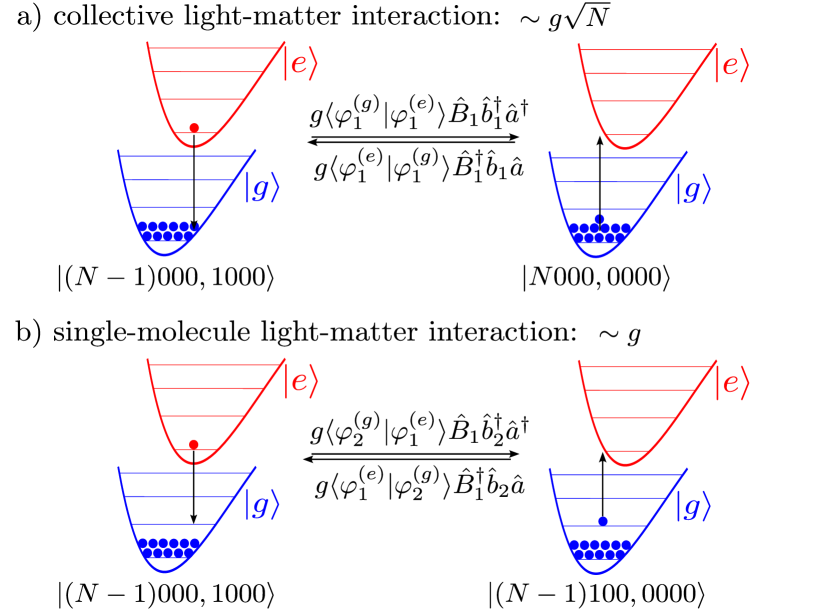
Consider an initial state with molecules in the global ground state and a single excited molecule (zero temperature), i.e., . We can obtain intuition about the dynamics of the excited molecule in the cavity by analyzing the light-matter coupling terms between and the other many-body basis states. Notably, light-matter couplings that destroy the excited state molecule while creating a cavity photon and a molecule at the macroscopically occupied global ground state are amplified by a factor of , while light-matter couplings that create molecules in the unoccupied vibrationally excited states of the ground electronic state are not (see Fig. 2). This collective light-matter interaction can be understood as a consequence of bosonic stimulation, although it can also be thought of as a consequence of the constructive interference of emission pathways for all the molecules when starting with a permutationally-symmetric excited state Pérez-Sánchez et al. (2023).
The clear disparity between collective and single-molecule coupling strengths in the large limit motivates a partitioning of the bosonic molecular polariton Hamiltonian as , with
| (6) |
This partitioning will be instrumental in the next sections.
Naturally, a large number of cavity photons can enhance the light-matter interaction as well (e.g., via stimulated emission). So care must be taken when utilizing this partitioning when a large number of excitations are present.
IV Quantum dynamics in the first excitation manifold
Here we focus on the Hilbert subspace with . This so-called first excitation manifold describes the system containing a single excitation either as a photon or as an electronic excitation. This regime is very important as it describes approximately the polariton system being irradiated by a weak laser Cui, Sukharev, and Nitzan (2023) (the linear regime in the external laser field).
Our method, called collective dynamics using truncated equations (CUT-E) Pérez-Sánchez et al. (2023), was developed to study the first-excitation manifold. At the heart of the method is the observation that the collective couplings are much larger than the single-molecule counterparts (). CUT-E reveals a structure of the equations of motion of the molecular polariton system that allows for their systematic truncation. Our original derivation was carried out in the language of first quantization; here, we provide a new and simpler derivation using the bosonic representation discussed in the previous sections. For simplicity, let us use the multi-particle states notation introduced by Philpott Philpott (1971) in the context of electronic spectra of molecular aggregates, which has been used to describe molecular polaritons previously by Herrera and Spano Herrera and Spano (2017),
| (7) |
Next, we notice that the molecular polariton Hamiltonian of Eq. II.2 becomes block-tridiagonal in this basis (see Appendix B),
| (8) |
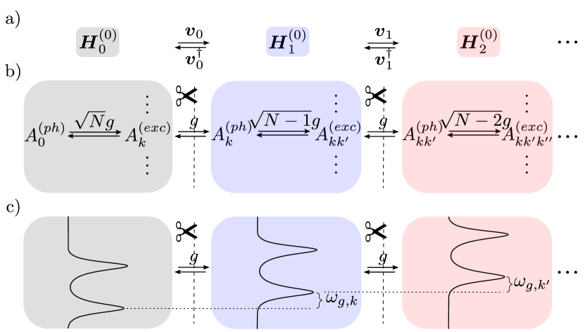
Here, we have used the partitioning of the Hamiltonian in Eq. III, where all collective light-matter couplings are contained inside each block , while the single-molecule light-matter interaction couple neighboring blocks. The subscript corresponds to the number of electronic ground state molecules with vibrational excitations, and we refer to it as a quasi-conserved quantity. In other words, only vibrational excitations in electronic ground state molecules can be created only via the (small) single-molecule light-matter coupling . The states and form a complete basis set for , the states and form a complete basis set for , and so on.
The CUT-E method approximates the polariton dynamics by truncating the basis of the ansatz wavefunction
| (9) |
For instance, if only collective light-matter coupling terms are to be accounted for, only the first two terms in the RHS of Eq. IV must be included in the ansatz wavefunction. We call this zeroth-order CUT-E. On the other hand, if at least one action of the single-molecule coupling is to be considered, the first four terms must be included. We call this first-order CUT-E. This hierarchy is summarized in the scheme of Fig. 3.
IV.1 The limit
A simple solution to the molecular polariton dynamics is obtained by taking the limit when (or ) while keeping the collective coupling constant. In this case, the Hamiltonian in Eq. 8 becomes block diagonal, and the problem is trivially solved by diagonalizing each block separately. The eigenstates of these blocks can be used as reference states from which the exact eigenstates for finite can be approximated. As an illustrative example, let us analyze the zeroth block (hereafter ),
| (10) |
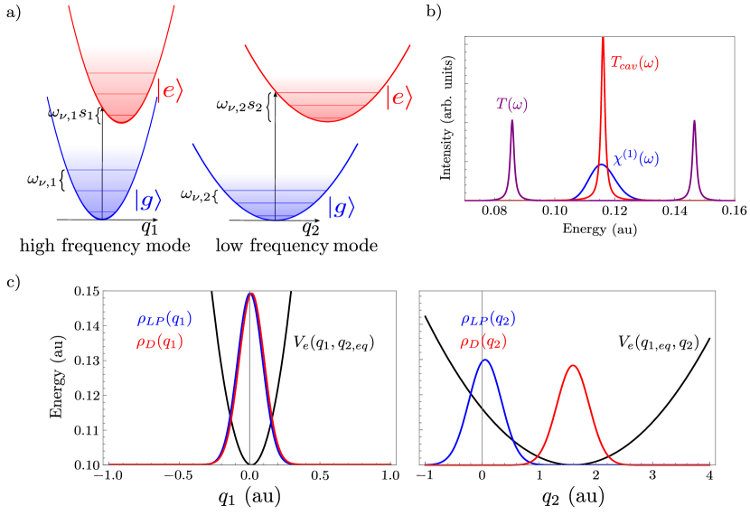
In this picture, the vibro-polaritonic eigenstates of with a high and negligible photonic character are called “polariton” and “dark states” states, respectively. Polaritons typically have a large contribution from the bright state and form two bands known as the upper (high frequency) and lower (low frequency) polaritons. On the other hand, dark states are Stokes-shifted states that remain at their original energies outside the cavity (see Fig 4b).
Besides the obvious simplification obtained by having to calculate the eigenstates of only a single block, using to model the polaritonic system is equivalent to using classical linear optics treatments, where the photonic mode of frequency is strongly coupled to a set of effective oscillators representing the electronic transitions of the bare molecule with frequencies , which can be obtained from the linear response of the bare molecular ensemble Ćwik et al. (2016); Zeb, Kirton, and Keeling (2018b); Yuen-Zhou and Koner (2024); Lieberherr et al. (2023). In fact, it was recently pointed out that the molecular dynamics under can be reproduced by a weak laser acting on the bare molecular ensemble Schwennicke et al. (2024). In the frequency domain, the polaritons act mainly as optical filters that allow only certain frequencies to enter the cavity and interact weakly with the molecular ensemble Schwennicke et al. (2024).
This theoretical prediction holds even in the presence of static disorder, where permutational symmetries are broken by small variations in the molecular environments. For CUT-E to be implemented in this scenario, we coarse-grain the disorder distribution and apply permutational symmetries to the molecules within each disorder bin. Since the ability of the cavity to resolve energetic differences between molecules depends on the propagation time, a relatively small number of disorder bins is needed to capture the ultrafast dynamics of the disorder ensemble, and we can take the limit where the number of molecules within each disorder bin goes to infinity Pérez-Sánchez et al. (2024b). Both the numerical convergence of the dynamics using this coarse-graining approach Sokolovskii, Morozov, and Groenhof (2024); Pérez-Sánchez et al. (2024b), and the optical filtering prediction Dutta et al. (2024) have been numerically tested in recent works. We believe a similar approach can be used to incorporate multiple cavity modes in the CUT-E formalism by coarse-graining the distribution of molecules in real space, which can open a path towards the efficient simulation of polariton transport and polariton condensation in the large limit. Recent theoretical works have already made significant progress in this direction Engelhardt and Cao (2023).
IV.2 corrections
From the previous discussion, it becomes clear that, within the limitations of this theory (e.g., no distance-dependent intermolecular interactions, finite temperature, etc), single-molecule light-matter coupling effects must be included in order to obtain polaritonic phenomena beyond those described by classical linear optics. Here, we show that these effects can be incorporated in a relatively simple manner using perturbation theory.
As an example, consider an initial state that lives in the zeroth block (e.g., a dark state or a polariton at zero temperature). Using the partitioning of the Hamiltonian in Eq. III, we can express the survival amplitude as a expansion:
| (11) |
Notice that, due to the choice of the initial state and the block-tridiagonal structure of the Hamiltonian, only even actions of are allowed. Moreover, each action of adds a factor of , meaning that the perturbative expansion leads to a expansion, with in Eq. IV.2 being .
Although numerical calculations of such corrections can be challenging, a simplification is allowed in the limit where . First, notice that the second block from Eq. 8 can be written as , with
| (12) |
Also, notice that the Hamiltonian in Eq. 12 differs from that in Eq. 10 in a constant energy shift by (the energy of the vibrational excitation in one ground state molecule), and in the reduced collective coupling . In the limit, we can approximate . This implies that only the eigenstates and eigenvalues of must be calculated to obtain the eigenstates of . A similar argument applies for all blocks as long as low-order corrections are needed (see Fig. 3c). Single-molecule coupling effects can be easily included via perturbation theory. The single-molecule light-matter coupling matrix , where the matrix that couples with the sub-block is given by
| (13) |
The perturbative approach in the limit was recently used to describe the radiative decay of dark states Michetti and La Rocca (2008); Coles et al. (2014); Michetti and La Rocca (2009); Coles et al. (2011). In first-order perturbation theory, we find the radiative pumping rate, ; while in second-order perturbation theory, we find the polariton-assisted Raman scattering rate, Pérez-Sánchez and Yuen-Zhou (2024). The existence of a expansion implies that there are additional rate contributions beyond whose underlying physical mechanisms have not been explored yet.
V CUT-E as a expansion
Studying the properties of physical systems in the limit where one of its parameters is taken to infinity, followed by the addition of corrections, is a common practice in quantum field theories Chatterjee (1990); Witten (1979, 1980) and the study of quantum-classical correspondence Prosen, Seligman, and Znidaric (2003); Morita (2022); Pappalardi, Polkovnikov, and Silva (2020); Hashimoto, Murata, and Yoshii (2017); Karnakov and Krainov (2013). For example, the limit where the number of field components approaches infinity Moshe and Zinn-Justin (2003) usually leads to a classical description where quantum fluctuations are suppressed (as in Sec. IV.1). Subsequently, corrections are systematically added to account for quantum fluctuations (as in Sec. IV.2). In electronic structure theory, classical electrostatics or mean-field theory become exact methods in the limit where the number of dimensions, electrons, and coordination number are taken to infinity Dunn et al. (1994); Vollhardt (2012); Metzner and Vollhardt (1989); Georges et al. (1996). In QCD, the number of colors is the parameter taken to infinity Hooft (1974); Manohar (1998). The linear harmonic regime in the large limit is also found in quantum impurity models Makri (1999), and in the Sachdev-Ye-Kitaev (SYK) Sachdev and Ye (1993); Kitaev (2015) and the Sherrington-Kirkpatrick Rosenhaus (2019); Pappalardi, Polkovnikov, and Silva (2020) models in many-body physics where plays the role of the effective Planck’s constant. By mapping the polaritons problem to a quantum impurity model, it can be shown that the dynamics of the photon mode in the large limit can be exactly captured by replacing the complex anharmonic molecular bath with a surrogate harmonic one (see Eq. 10) Yuen-Zhou and Koner (2024); Chin et al. (2010). In our CUT-E method, each term of the expansion has its origins in single-molecule light-matter coupling processes. CUT-E teaches us that there is still much we can learn from expansions for otherwise intractable chemical systems.
VI Quantum dynamics in high excitation manifolds
Generalization of CUT-E for excitation manifolds is paramount to describe experiments where the pump power is high enough to enter the non-linear regime in the external field. Some common scenarios involve polariton condensation Kasprzak et al. (2006); Kéna-Cohen and Forrest (2010); Mazza et al. (2013); Daskalakis et al. (2014); Plumhof et al. (2014); Grant et al. (2016); Pannir-Sivajothi et al. (2022) and non-linear spectroscopy of molecular polaritons Dunkelberger et al. (2016); Chervy et al. (2016); Xiang et al. (2018); Barachati et al. (2018); Renken et al. (2021); Cheng et al. (2022a, b); Hirschmann, Bhakta, and Xiong (2023).
As a first approximation, one may consider calculating the dynamics in higher excitation manifolds while still neglecting corrections of the single-molecule light-matter coupling. This regime is characterized as . For a fixed value of and assuming a zero temperature initial state (all molecules in the electronic ground state are in the vibrational state ), the relevant Hamiltonian can be written as a block tri-diagonal matrix
| (14) |
Here, corresponds to all states with ground state molecules vibrationally excited, and photons in the cavity mode. This is a generalization of Eq. 10 for . Since is the collective coupling, it cannot be treated perturbatively, leading to high computational costs for large .
A much more natural approach is to express the photon and matter annihilation operators as
| (15) |
followed by the use of the Truncated-Wigner-Approximation Wigner (1932); Phuc (2024) or the Meyer-Miller mappings toolbox Meyer and Miller (2008); Stock and Thoss (1997); Ananth, Venkataraman, and Miller (2007); Sun, Sasmal, and Vendrell (2021); Richardson and Thoss (2013); Hu et al. (2022).
It is important to emphasize that Eq. 14 alone corresponds to a well-defined (e.g., starting with a Fock state of photons), a situation that differs from when the initial state corresponds to a largely occupied photon coherent state, which is typically the case in experiments. Future works will focus on adapting Eq. 14 to the study of molecular polaritons in high excitation regimes that are experimentally relevant, as well as its comparison with other currently available theories that work in the same regime Fowler-Wright, Lovett, and Keeling (2022); Zeb, Kirton, and Keeling (2022); Pizzi et al. (2023).
VII Summary
The collective dynamics using truncated equations (CUT-E) formalism was developed to efficiently compute the quantum dynamics of molecular polariton systems. Here, we re-derived and re-interpreted CUT-E in light of recent theoretical advances in the field. Specifically, we provided a simpler derivation using the Schwinger boson representation of the polariton Hamiltonian, which was introduced in recent studies. We also revisited the limit, where the system can be described using classical linear optics, and for the first time showed that corrections for finite can be expressed as a series. This allowed us to formally establish CUT-E as a expansion method for the many-body dynamics of molecular polaritons. Lastly, we outlined a path forward for simulating polariton dynamics in highly excited states, enabling efficient simulations of experiments like polariton condensation and nonlinear spectroscopy.
Acknowledgements.
This work was supported by the Air Force Office of Scientific Research (AFOSR) through the Multi-University Research Initiative (MURI) program no. FA9550-22-1-0317.Data Availability Statement
Data sharing is not applicable – no new data is generated
Appendix A Schwinger boson representation of molecular polaritons
Consider a system of identical non-interacting molecules collectively coupled to a single cavity mode. The Tavis-Cummings Hamiltonian, extended to include vibrational degrees of freedom, can be written as
| (16) |
We can represent the first-quantized many-body wavefunction of the system using a complete basis of single-particle wavefunctions for each of the molecules in the ensemble, and the Fock state basis states for the photon mode. The time-dependent wavefunction in this basis is given by
| (17) |
If we impose a permutationally-symmetric initial wavefunction, such symmetry will be conserved under time evolution since the Hamiltonian is permutationally invariant. Hence, we can write
| (18) |
This implies that the dynamics of the system can be computed in a permutationally-symmetric subspace of the entire Hilbert space. An example of a permutationally-symmetric state is all molecules in the global ground state (zero temperature). In terms of the bosonic symmetrization operator, we get
| (19) |
where is defined by the permanent
| (20) |
At this point, it is clear that we can use the second quantization formalism, just like we do for bosonic particles. This approach avoids the complex symmetrization and renormalization procedures needed in first quantization when dealing with the many-body wavefunction. Those procedures arise from asking the wrong question: what is the state of each individual molecule at any given time? Since the molecules are indistinguishable from the outset, we should instead ask how many molecules are in each single-particle state.
In the second-quantized picture this information is included in the many body states , with being the number of molecules occupying the state .
To map operators to the second-quantized picture, we use bosonic creation and annihilation operators and . Analogue operators acting on the first-quantized many-body wavefunction delete or insert a single-particle state while conserving its symmetrization. Acting on the second-quantized many-body wavefunction, and will lower and increase the occupation in the single-particle state by one, respectively; they destroy and create molecules in the single-particle states . Moreover, we can map any symmetric sum of single-particle operators, , from the first-quantized to the second-quantized picture, using the creation and annihilation operators via Bruus and Flensberg (2004)
| (21) |
Using the vibronic eigenstates and as the basis set, and the mapping between first- and second-quantized operators above, we can obtain the molecular polariton Hamiltonian in Eq. II.2 of the manuscript.
Appendix B Block-tridigonal structure of the molecular polariton Hamiltonian
The molecular polariton Hamiltonian in Eq. II.2 can be partitioned as
| (22) |
where contains the collective light-matter couplings while the perturbation accounts for all single-molecule light-matter couplings.
Notice that commutes with the operators , i.e., the number of molecules in the electronic ground state in each vibrational excited state. This implies that can be written as a block-diagonal matrix of the form
| (23) |
Likewise, can also be written as a block-diagonal matrix where each block represents a distribution of the molecules amongst all excited vibrational excited states. For example, for we have
| (24) |
Notice that does not commute with the perturbation . Based on this, we refer to the number of ground state molecules in each vibrationally excited state as a quasi-conserved quantity. In other words, collective light-matter coupling cannot create or destroy phonons in electronic ground-state molecules. Finally, notice that the perturbation can only create or destroy one ground-state molecule with vibrational excitations at a time. This gives the molecular polariton Hamiltonian in Eq. 8 its block-tridiagonal structure.
References
- Ribeiro et al. (2018) R. F. Ribeiro, L. A. Martínez-Martínez, M. Du, J. Campos-Gonzalez-Angulo, and J. Yuen-Zhou, “Polariton chemistry: controlling molecular dynamics with optical cavities,” Chem. Sci. 9, 6325–6339 (2018).
- Ebbesen, Rubio, and Scholes (2023) T. W. Ebbesen, A. Rubio, and G. D. Scholes, “Introduction: Polaritonic chemistry,” Chem. Rev. 123, 12037–12038 (2023).
- Xiong (2023) W. Xiong, “Molecular vibrational polariton dynamics: What can polaritons do?” Acc. Chem. Res. 56, 776–786 (2023).
- Bhuyan et al. (2023) R. Bhuyan, J. Mony, O. Kotov, G. W. Castellanos, J. Gómez Rivas, T. O. Shegai, and K. Börjesson, “The rise and current status of polaritonic photochemistry and photophysics,” Chem. Rev. 123, 10877–10919 (2023).
- Mandal et al. (2023) A. Mandal, M. A. Taylor, B. M. Weight, E. R. Koessler, X. Li, and P. Huo, “Theoretical advances in polariton chemistry and molecular cavity quantum electrodynamics,” Chem. Rev. 123, 9786–9879 (2023).
- Xiang and Xiong (2024) B. Xiang and W. Xiong, “Molecular polaritons for chemistry, photonics and quantum technologies,” Chem. Rev. 124, 2512–2552 (2024).
- Coles et al. (2014) D. M. Coles, N. Somaschi, P. Michetti, C. Clark, P. G. Lagoudakis, P. G. Savvidis, and D. G. Lidzey, “Polariton-mediated energy transfer between organic dyes in a strongly coupled optical microcavity,” Nat. Mater. 13, 712–719 (2014).
- Reitz, Mineo, and Genes (2018) M. Reitz, F. Mineo, and C. Genes, “Energy transfer and correlations in cavity-embedded donor-acceptor configurations,” Sci. Rep. 8, 9050 (2018).
- DelPo et al. (2021) C. A. DelPo, S.-U.-Z. Khan, K. H. Park, B. Kudisch, B. P. Rand, and G. D. Scholes, “Polariton decay in donor–acceptor cavity systems,” J. Phys. Chem. Lett. 12, 9774–9782 (2021).
- Martínez-Martínez et al. (2018) L. A. Martínez-Martínez, M. Du, R. F. Ribeiro, S. Kéna-Cohen, and J. Yuen-Zhou, “Polariton-assisted singlet fission in acene aggregates,” J. Phys. Chem. Lett. 9, 1951–1957 (2018).
- Xiang et al. (2020) B. Xiang, R. F. Ribeiro, M. Du, L. Chen, Z. Yang, J. Wang, J. Yuen-Zhou, and W. Xiong, “Intermolecular vibrational energy transfer enabled by microcavity strong light–matter coupling,” Science 368, 665–667 (2020).
- Koner et al. (2023) A. Koner, M. Du, S. Pannir-Sivajothi, R. H. Goldsmith, and J. Yuen-Zhou, “A path towards single molecule vibrational strong coupling in a fabry–pérot microcavity,” Chem. Sci. 14, 7753–7761 (2023).
- Peng and Rabani (2024) K. Peng and E. Rabani, “Polariton assisted incoherent to coherent excitation energy transfer between colloidal nanocrystal quantum dots,” (2024), arXiv:2406.09642 [cond-mat.mes-hall] .
- Hutchison et al. (2012) J. A. Hutchison, T. Schwartz, C. Genet, E. Devaux, and T. W. Ebbesen, “Modifying chemical landscapes by coupling to vacuum fields,” Angew. Chem., Int. Ed. Engl. 51, 1592–1596 (2012).
- Dunkelberger et al. (2016) A. Dunkelberger, B. Spann, K. Fears, B. Simpkins, and J. Owrutsky, “Modified relaxation dynamics and coherent energy exchange in coupled vibration-cavity polaritons,” Nat. Commun. 7, 13504 (2016).
- Zeng et al. (2023) H. Zeng, J. B. Pérez-Sánchez, C. T. Eckdahl, P. Liu, W. J. Chang, E. A. Weiss, J. A. Kalow, J. Yuen-Zhou, and N. P. Stern, “Control of photoswitching kinetics with strong light–matter coupling in a cavity,” J. Am. Chem. Soc. 145, 19655–19661 (2023).
- Dunkelberger et al. (2022) A. D. Dunkelberger, B. S. Simpkins, I. Vurgaftman, and J. C. Owrutsky, “Vibration-cavity polariton chemistry and dynamics,” Annu. Rev. Phys. Chem. 73, 429–451 (2022).
- Nelson and Weichman (2024) J. C. Nelson and M. L. Weichman, “More than just smoke and mirrors: Gas-phase polaritons for optical control of chemistry,” J. Chem. Phys. 161 (2024), 10.1063/5.0220077.
- Ishii et al. (2022) T. Ishii, K. Miyata, M. Mamada, F. Bencheikh, F. Mathevet, K. Onda, S. Kéna-Cohen, and C. Adachi, “Low-threshold exciton-polariton condensation via fast polariton relaxation in organic microcavities,” Adv. Opt. Mater. 10, 2102034 (2022).
- Kéna-Cohen and Forrest (2010) S. Kéna-Cohen and S. Forrest, “Room-temperature polariton lasing in an organic single-crystal microcavity,” Nat. Photon. 4, 371–375 (2010).
- Luk et al. (2017) H. L. Luk, J. Feist, J. J. Toppari, and G. Groenhof, “Multiscale molecular dynamics simulations of polaritonic chemistry,” J. Chem. Theory Comp. 13, 4324–4335 (2017).
- Groenhof et al. (2019) G. Groenhof, C. Climent, J. Feist, D. Morozov, and J. J. Toppari, “Tracking polariton relaxation with multiscale molecular dynamics simulations,” J. Phys. Chem. Lett. 10, 5476–5483 (2019).
- Li, Nitzan, and Subotnik (2022) T. E. Li, A. Nitzan, and J. E. Subotnik, “Energy-efficient pathway for selectively exciting solute molecules to high vibrational states via solvent vibration-polariton pumping,” Nat. Commun. 13, 4203 (2022).
- Li and Hammes-Schiffer (2023) T. E. Li and S. Hammes-Schiffer, “Qm/mm modeling of vibrational polariton induced energy transfer and chemical dynamics,” J. Am. Chem. Soc. 145, 377–384 (2023).
- Sidler et al. (2021) D. Sidler, C. Schäfer, M. Ruggenthaler, and A. Rubio, “Polaritonic chemistry: Collective strong coupling implies strong local modification of chemical properties,” J. Phys. Chem. Lett. 12, 508–516 (2021).
- Sidler et al. (2022) D. Sidler, M. Ruggenthaler, C. Schäfer, E. Ronca, and A. Rubio, “A perspective on ab initio modeling of polaritonic chemistry: The role of non-equilibrium effects and quantum collectivity,” J. Chem. Phys. 156, 230901 (2022).
- Schäfer (2022) C. Schäfer, “Polaritonic chemistry from first principles via embedding radiation reaction,” J. Phys. Chem. Lett. 13, 6905–6911 (2022).
- El Moutaoukal et al. (0) Y. El Moutaoukal, R. R. Riso, M. Castagnola, and H. Koch, “Toward polaritonic molecular orbitals for large molecular systems,” J. Chem. Theory Comp. 0, null (0).
- Pérez-Sánchez et al. (2023) J. B. Pérez-Sánchez, A. Koner, N. P. Stern, and J. Yuen-Zhou, “Simulating molecular polaritons in the collective regime using few-molecule models,” Proc. Natl. Acad. Sci. USA. 120, e2219223120 (2023).
- Witten (1979) E. Witten, “Instatons, the quark model, and the 1/n expansion,” Nucl. Phys. B 149, 285–320 (1979).
- Hooft (1974) G. Hooft, “A planar diagram theory for strong interactions,” Nucl. Phys. B 72, 461–473 (1974).
- Chatterjee (1990) A. Chatterjee, “Large- n expansions in quantum mechanics, atomic physics and some o invariant systems,” Phys. Rep. 186, 249–370 (1990).
- Witten (1980) E. Witten, “Quarks, atoms, and the 1/N expansion,” Phys. Today 33, 38–43 (1980).
- Vollhardt (2012) D. Vollhardt, “Dynamical mean-field theory for correlated electrons,” Ann. Phys. 524, 1–19 (2012).
- Zeb, Kirton, and Keeling (2018a) M. A. Zeb, P. G. Kirton, and J. Keeling, “Exact states and spectra of vibrationally dressed polaritons,” ACS Photonics 5, 249–257 (2018a).
- Fowler-Wright, Lovett, and Keeling (2022) P. Fowler-Wright, B. W. Lovett, and J. Keeling, “Efficient many-body non-markovian dynamics of organic polaritons,” Phys. Rev. Lett. 129, 173001 (2022).
- Cui and Nizan (2022) B. Cui and A. Nizan, “Collective response in light–matter interactions: The interplay between strong coupling and local dynamics,” J. Chem. Phys. 157, 114108 (2022).
- Zeb, Kirton, and Keeling (2022) M. A. Zeb, P. G. Kirton, and J. Keeling, “Incoherent charge transport in an organic polariton condensate,” Phys. Rev. B 106, 195109 (2022).
- Gu (2023) B. Gu, “Toward collective chemistry by strong light-matter coupling,” (2023), arXiv:2306.08944 [quant-ph] .
- Sidler, Ruggenthaler, and Rubio (2024) D. Sidler, M. Ruggenthaler, and A. Rubio, “The connection of polaritonic chemistry with the physics of a spin glass,” (2024), arXiv:2409.08986 [physics.chem-ph] .
- Lindoy, Mandal, and Reichman (2024) L. P. Lindoy, A. Mandal, and D. R. Reichman, “Investigating the collective nature of cavity-modified chemical kinetics under vibrational strong coupling,” Nanophotonics 13, 2617–2633 (2024).
- Pérez-Sánchez et al. (2024a) J. B. Pérez-Sánchez, F. Mellini, J. Yuen-Zhou, and N. C. Giebink, “Collective polaritonic effects on chemical dynamics suppressed by disorder,” Phys. Rev. Res. 6, 013222 (2024a).
- Yuen-Zhou and Koner (2024) J. Yuen-Zhou and A. Koner, “Linear response of molecular polaritons,” J. Chem. Phys. 160, 154107 (2024).
- Pérez-Sánchez and Yuen-Zhou (2024) J. B. Pérez-Sánchez and J. Yuen-Zhou, “Radiative pumping vs vibrational relaxation of molecular polaritons: a bosonic mapping approach,” (2024), arXiv:2407.20594 [quant-ph] .
- Schwennicke et al. (2024) K. Schwennicke, A. Koner, J. B. Pérez-Sánchez, W. Xiong, N. C. Giebink, M. L. Weichman, and J. Yuen-Zhou, “When do molecular polaritons behave like optical filters?” (2024), arXiv:2408.05036 [physics.chem-ph] .
- Gegg and Richter (2016) M. Gegg and M. Richter, “Efficient and exact numerical approach for many multi-level systems in open system cqed,” New J. Phys. 18, 043037 (2016).
- Shammah et al. (2018) N. Shammah, S. Ahmed, N. Lambert, S. De Liberato, and F. Nori, “Open quantum systems with local and collective incoherent processes: Efficient numerical simulations using permutational invariance,” Phys. Rev. A 98, 063815 (2018).
- Zeb (2022a) M. A. Zeb, “Efficient linear scaling mapping for permutation symmetric fock spaces,” Comp. Phys. Commun. 276, 108347 (2022a).
- Silva and Feist (2022) R. E. F. Silva and J. Feist, “Permutational symmetry for identical multilevel systems: A second-quantized approach,” Phys. Rev. A 105, 043704 (2022).
- Pizzi et al. (2023) A. Pizzi, A. Gorlach, N. Rivera, A. Nunnenkamp, and I. Kaminer, “Light emission from strongly driven many-body systems,” Nat. Phys. 19, 551–561 (2023).
- Sukharnikov et al. (2023) V. Sukharnikov, S. Chuchurka, A. Benediktovitch, and N. Rohringer, “Second quantization of open quantum systems in liouville space,” Phys. Rev. A 107, 053707 (2023).
- Biedenharn and Van Dam (1965) L. Biedenharn and H. Van Dam, Quantum Theory of Angular Momentum: A Collection of Reprints and Original Papers, Perspectives in Physics: a Series of Reprint Collections (Academic Press, 1965).
- Zeb (2022b) M. A. Zeb, “Efficient linear scaling mapping for permutation symmetric fock spaces,” Comp. Phys. Commun. 276, 108347 (2022b).
- Cui, Sukharev, and Nitzan (2023) B. Cui, M. Sukharev, and A. Nitzan, “Comparing semiclassical mean-field and 1-exciton approximations in evaluating optical response under strong light–matter coupling conditions,” J. Chem. Phys. 158, 164113 (2023), https://pubs.aip.org/aip/jcp/article-pdf/doi/10.1063/5.0146984/17060482/164113_1_5.0146984.pdf .
- Philpott (1971) M. R. Philpott, “Theory of the Coupling of Electronic and Vibrational Excitations in Molecular Crystals and Helical Polymers,” J. Chem. Phys. 55, 2039–2054 (1971).
- Herrera and Spano (2017) F. Herrera and F. C. Spano, “Dark vibronic polaritons and the spectroscopy of organic microcavities,” Phys. Rev. Lett. 118, 223601 (2017).
- Ćwik et al. (2016) J. A. Ćwik, P. Kirton, S. De Liberato, and J. Keeling, “Excitonic spectral features in strongly coupled organic polaritons,” Phys. Rev. A 93, 033840 (2016).
- Zeb, Kirton, and Keeling (2018b) M. A. Zeb, P. G. Kirton, and J. Keeling, “Exact states and spectra of vibrationally dressed polaritons,” ACS Photonics 5, 249–257 (2018b).
- Lieberherr et al. (2023) A. Z. Lieberherr, S. T. E. Furniss, J. E. Lawrence, and D. E. Manolopoulos, “Vibrational strong coupling in liquid water from cavity molecular dynamics,” J. Chem. Phys. 158, 234106 (2023).
- Pérez-Sánchez et al. (2024b) J. B. Pérez-Sánchez, F. Mellini, J. Yuen-Zhou, and N. C. Giebink, “Collective polaritonic effects on chemical dynamics suppressed by disorder,” Phys. Rev. Res. 6, 013222 (2024b).
- Sokolovskii, Morozov, and Groenhof (2024) I. Sokolovskii, D. Morozov, and G. Groenhof, “One molecule to couple them all: Toward realistic numbers of molecules in multiscale molecular dynamics simulations of exciton-polaritons,” J. Chem. Phys. 161, 134106 (2024).
- Dutta et al. (2024) A. Dutta, V. Tiainen, I. Sokolovskii, L. Duarte, N. Markešević, D. Morozov, H. A. Qureshi, S. Pikker, G. Groenhof, and J. J. Toppari, “Thermal disorder prevents the suppression of ultra-fast photochemistry in the strong light-matter coupling regime,” Nat. Commun. 15, 6600 (2024).
- Engelhardt and Cao (2023) G. Engelhardt and J. Cao, “Polariton localization and dispersion properties of disordered quantum emitters in multimode microcavities,” Phys. Rev. Lett. 130, 213602 (2023).
- Michetti and La Rocca (2008) P. Michetti and G. C. La Rocca, “Simulation of j-aggregate microcavity photoluminescence,” Phys. Rev. B 77, 195301 (2008).
- Michetti and La Rocca (2009) P. Michetti and G. C. La Rocca, “Exciton-phonon scattering and photoexcitation dynamics in -aggregate microcavities,” Phys. Rev. B 79, 035325 (2009).
- Coles et al. (2011) D. M. Coles, P. Michetti, C. Clark, W. C. Tsoi, A. M. Adawi, J.-S. Kim, and D. G. Lidzey, “Vibrationally assisted polariton-relaxation processes in strongly coupled organic-semiconductor microcavities,” Adv. Funct. Mater. 21, 3691–3696 (2011).
- Prosen, Seligman, and Znidaric (2003) T. Prosen, T. Seligman, and M. Znidaric, “Theory of quantum loschmidt echoes,” Prog. Theor. Phys. 150 (2003), 10.1143/PTPS.150.200.
- Morita (2022) T. Morita, “Extracting classical lyapunov exponent from one-dimensional quantum mechanics,” Phys. Rev. D 106, 106001 (2022).
- Pappalardi, Polkovnikov, and Silva (2020) S. Pappalardi, A. Polkovnikov, and A. Silva, “Quantum echo dynamics in the Sherrington-Kirkpatrick model,” SciPost Phys. 9, 021 (2020).
- Hashimoto, Murata, and Yoshii (2017) K. Hashimoto, K. Murata, and R. Yoshii, “Out-of-time-order correlators in quantum mechanics,” J. High Energy Phys. 2017, 138 (2017).
- Karnakov and Krainov (2013) B. M. Karnakov and V. P. Krainov, “1/N-expansion in quantum mechanics,” in WKB Approximation in Atomic Physics (Springer Berlin Heidelberg, Berlin, Heidelberg, 2013) pp. 31–55.
- Moshe and Zinn-Justin (2003) M. Moshe and J. Zinn-Justin, “Quantum field theory in the large n limit: a review,” Phys. Rep. 385, 69–228 (2003).
- Dunn et al. (1994) M. Dunn, T. C. Germann, D. Z. Goodson, C. A. Traynor, I. Morgan, John D., D. K. Watson, and D. R. Herschbach, “A linear algebraic method for exact computation of the coefficients of the 1/D expansion of the Schrödinger equation,” J. Chem. Phys. 101, 5987–6004 (1994).
- Metzner and Vollhardt (1989) W. Metzner and D. Vollhardt, “Correlated lattice fermions in dimensions,” Phys. Rev. Lett. 62, 324–327 (1989).
- Georges et al. (1996) A. Georges, G. Kotliar, W. Krauth, and M. J. Rozenberg, “Dynamical mean-field theory of strongly correlated fermion systems and the limit of infinite dimensions,” Rev. Mod. Phys. 68, 13–125 (1996).
- Manohar (1998) A. V. Manohar, “Large n qcd,” (1998), arXiv:hep-ph/9802419 [hep-ph] .
- Makri (1999) N. Makri, “The linear response approximation and its lowest order corrections: An influence functional approach,” J. Phys. Chem. B 103, 2823–2829 (1999).
- Sachdev and Ye (1993) S. Sachdev and J. Ye, “Gapless spin-fluid ground state in a random quantum heisenberg magnet,” Phys. Rev. Lett. 70, 3339–3342 (1993).
- Kitaev (2015) A. Kitaev, “A simple model of quantum holography,” Talk at KITP Program: Entanglement in Strongly-Correlated Quantum Matter, online videos: http://online.kitp.ucsb.edu/online/entangled15/kitaev/ (Part 1) and http://online.kitp.ucsb.edu/online/entangled15/kitaev2/ (Part 2) (2015), online talks.
- Rosenhaus (2019) V. Rosenhaus, “An introduction to the syk model,” J. Phys. A: Math. Theor. 52, 323001 (2019).
- Chin et al. (2010) A. W. Chin, A. Rivas, S. F. Huelga, and M. B. Plenio, “Exact mapping between system-reservoir quantum models and semi-infinite discrete chains using orthogonal polynomials,” J. Math. Phys. 51, 092109 (2010).
- Kasprzak et al. (2006) J. Kasprzak, M. Richard, S. Kundermann, A. Baas, P. Jeambrun, J. M. J. Keeling, F. Marchetti, M. Szymańska, R. André, J. Staehli, et al., “Bose–einstein condensation of exciton polaritons,” Nature 443, 409–414 (2006).
- Mazza et al. (2013) L. Mazza, S. Kéna-Cohen, P. Michetti, and G. C. La Rocca, “Microscopic theory of polariton lasing via vibronically assisted scattering,” Phys. Rev. B 88, 075321 (2013).
- Daskalakis et al. (2014) K. Daskalakis, S. Maier, R. Murray, and S. Kéna-Cohen, “Nonlinear interactions in an organic polariton condensate,” Nat. Mater. 13, 271–278 (2014).
- Plumhof et al. (2014) J. D. Plumhof, T. Stöferle, L. Mai, U. Scherf, and R. F. Mahrt, “Room-temperature bose–einstein condensation of cavity exciton–polaritons in a polymer,” Nat. Mater. 13, 247–252 (2014).
- Grant et al. (2016) R. T. Grant, P. Michetti, A. J. Musser, P. Gregoire, T. Virgili, E. Vella, M. Cavazzini, K. Georgiou, F. Galeotti, C. Clark, et al., “Efficient radiative pumping of polaritons in a strongly coupled microcavity by a fluorescent molecular dye,” Adv. Opt. Mater. 4, 1615–1623 (2016).
- Pannir-Sivajothi et al. (2022) S. Pannir-Sivajothi, J. A. Campos-Gonzalez-Angulo, L. A. Martínez-Martínez, S. Sinha, and J. Yuen-Zhou, “Driving chemical reactions with polariton condensates,” Nat. Commun. 13, 1645 (2022).
- Chervy et al. (2016) T. Chervy, J. Xu, Y. Duan, C. Wang, L. Mager, M. Frerejean, J. A. W. Münninghoff, P. Tinnemans, J. A. Hutchison, C. Genet, A. E. Rowan, T. Rasing, and T. W. Ebbesen, “High-efficiency second-harmonic generation from hybrid light-matter states,” Nano Lett. 16, 7352–7356 (2016).
- Xiang et al. (2018) B. Xiang, R. F. Ribeiro, A. D. Dunkelberger, J. Wang, Y. Li, B. S. Simpkins, J. C. Owrutsky, J. Yuen-Zhou, and W. Xiong, “Two-dimensional infrared spectroscopy of vibrational polaritons,” Proc. Natl. Acad. Sci. USA. 115, 4845–4850 (2018).
- Barachati et al. (2018) F. Barachati, J. Simon, Y. A. Getmanenko, S. Barlow, S. R. Marder, and S. Kéna-Cohen, “Tunable third-harmonic generation from polaritons in the ultrastrong coupling regime,” ACS Photonics 5, 119–125 (2018).
- Renken et al. (2021) S. Renken, R. Pandya, K. Georgiou, R. Jayaprakash, L. Gai, Z. Shen, D. G. Lidzey, A. Rao, and A. J. Musser, “Untargeted effects in organic exciton–polariton transient spectroscopy: A cautionary tale,” J. Chem. Phys. 155 (2021).
- Cheng et al. (2022a) C.-Y. Cheng, N. Krainova, A. N. Brigeman, A. Khanna, S. Shedge, C. Isborn, J. Yuen-Zhou, and N. C. Giebink, “Molecular polariton electroabsorption,” Nat. Commun. 13, 7937 (2022a).
- Cheng et al. (2022b) C.-Y. Cheng, N. Krainova, A. N. Brigeman, A. Khanna, S. Shedge, C. Isborn, J. Yuen-Zhou, and N. C. Giebink, “Molecular polariton electroabsorption,” Nat. Commun. 13, 7937 (2022b).
- Hirschmann, Bhakta, and Xiong (2023) O. Hirschmann, H. H. Bhakta, and W. Xiong, “The role of ir inactive mode in w(co)6 polariton relaxation process,” Nanophotonics (2023), doi:10.1515/nanoph-2023-0589.
- Wigner (1932) E. Wigner, “On the quantum correction for thermodynamic equilibrium,” Phys. Rev. 40, 749–759 (1932).
- Phuc (2024) N. T. Phuc, “Semiclassical truncated-wigner-approximation theory of molecular vibration-polariton dynamics in optical cavities,” J. Chem. Theory Comput. 20, 3019–3027 (2024).
- Meyer and Miller (2008) H. Meyer and W. H. Miller, “Analysis and extension of some recently proposed classical models for electronic degrees of freedom,” J. Chem. Phys. 72, 2272–2281 (2008).
- Stock and Thoss (1997) G. Stock and M. Thoss, “Semiclassical description of nonadiabatic quantum dynamics,” Phys. Rev. Lett. 78, 578–581 (1997).
- Ananth, Venkataraman, and Miller (2007) N. Ananth, C. Venkataraman, and W. H. Miller, “Semiclassical description of electronically nonadiabatic dynamics via the initial value representation,” J. Chem. Phys. 127, 084114 (2007).
- Sun, Sasmal, and Vendrell (2021) J. Sun, S. Sasmal, and O. Vendrell, “A bosonic perspective on the classical mapping of fermionic quantum dynamics,” J. Chem. Phys. 155, 134110 (2021).
- Richardson and Thoss (2013) J. O. Richardson and M. Thoss, “Communication: Nonadiabatic ring-polymer molecular dynamics,” J. Chem. Phys. 139, 031102 (2013).
- Hu et al. (2022) D. Hu, A. Mandal, B. M. Weight, and P. Huo, “Quasi-diabatic propagation scheme for simulating polariton chemistry,” J. Chem. Phys. 157, 194109 (2022).
- Bruus and Flensberg (2004) H. Bruus and K. Flensberg, Many-body quantum theory in condensed matter physics: an introduction (OUP Oxford, 2004).