Inverter Output Impedance Estimation in Power Networks: A Variable Direction Forgetting Recursive-Least-Square Algorithm Based Approach

Abstract

As inverter-based loads and energy sources become increasingly prevalent, accurate line impedance estimation between inverters and the grid is essential for optimizing performance and enhancing control strategies. This paper presents a non-invasive estimation algorithm that avoids signal injection, based on the Variable Direction Forgetting Recursive Least Squares (VDF-RLS) method. The method uses measurement data that is local to the inverter. It proposes a specific method for determining rotational frequency for direct-quadrature (dq) coordinate frame in which data is collected, which ensures a simpler and more accurate estimation. This method is enabled by a secondary Phase Locked Loop (PLL) which appropriately attenuates the effects of variations in grid-voltage measurements. By isolating the variation-sensitive q-axis and relying solely on the less sensitive d-axis, the method further minimizes the impact of variations. The estimation method achieves rapid adaptation while ensuring stability in the absence of persistent excitation by selectively discarding outdated data during updates. Results demonstrate significant improvement (as large as $7$ times) in estimation of line parameters, when compared to existing approaches such as constant forgetting RLS.

I INTRODUCTION

The rapid growth of renewable energy technologies and the demand for greater accuracy in power transactions and voltage/frequency regulations have increased the adoption of inverter-based loads and energy sources like electric vehicles (EVs), photovoltaic (PV) systems, and battery energy storage systems (BESS). Understanding the interaction between these inverters and the grid has become a critical focus for research. A critical factor in this interaction is the output line impedance, which affects inverter performance, including power injection limits and droop control characteristics [1, 2]. Better impedance estimation, as noted in [3], allows for improved controller bandwidth. Line impedance also indicates grid stiffness and aids in detecting islanding events [4], helping inverters transition operational modes [5]. Accurate monitoring of these factors is vital for grid stability as inverter-based resources continue to grow.

This output impedance is often understood as the impedance between the inverter and the grid. Here the grid in the context of an inverter typically represents an abstraction of the remaining network. In a complex grid network setting, we model the grid experienced by the inverter using Thevenin’s theorem as a single grid voltage source and the output line impedance between the inverter and the voltage source. The impedance defined by Thevenin’s theorem can vary significantly with changes in the power network, such as fluctuations in electrical loads, the addition or removal of power sources, and even environmental factors like temperature. As a result, real-time estimation of line impedance becomes critical to optimizing the performance and reliability of inverters. This enables the system to adapt to dynamic grid conditions, ensuring stable power injection and updated control strategies.

A major challenge in accurately estimating the output line impedance stems from the fact that global measurements or network-wide information are typically unavailable to the inverter. Additionally, the measured signals often lack sufficient richness, meaning there is an absence of persistence of excitation, which is crucial for accurate estimation. Inverters typically operate at a steady point, where only the local output voltage and current are measurable, while both line impedance and grid voltage can influence these measurements.

Some methods, such as [6], assume that grid voltage information is accessible, simplifying the impedance estimation process. However, this assumption is often unrealistic. In large grids, where numerous loads, generators, and inverters are interconnected, it is difficult to pinpoint a location that accurately represents the grid voltage. Even if a measurement point is established, it might be located far from the inverter, introducing increased costs and time lags in data collection.

To overcome the challenges of limited excitation and the difficulty in measuring grid voltage, many line impedance estimation methods rely on signal injection techniques. In [7], a high-frequency signal is injected into the grid, assuming that the grid voltage contains only the nominal frequency component. This helps the estimation algorithm distinguish the effects of line impedance from those of the grid voltage. However, while effective in certain cases, this solution is often suboptimal because signal injection distorts the output voltage waveform, and tampering with power flow is either not allowed or not feasible. In [8], a method is proposed that utilizes the pulse-width modulation (PWM) signal as the injected signal. Since inverters already use PWM to convert DC to AC, this method avoids introducing additional distortion to the voltage or current. However, it requires fast sensing at a rate higher than the PWM switching frequency. Additionally, inverters are typically equipped with filters to reduce PWM-induced ripples, meaning the injected signal is very small, leading to a low signal-to-noise ratio (SNR). In [9], an alternative approach is taken that relies on time-domain differentiation rather than frequency-domain techniques. The inverter’s output power is slightly perturbed, under the assumption that the grid voltage remains constant during the perturbation. The resulting changes in the inverter’s voltage and current are attributed solely to the line impedance. However, these invasive, injection-based methods—along with concerns about voltage quality and power control—are often impractical, as such injections may not be permitted due to grid regulations or operational constraints.

Another important class of methods address the lack of persistence of excitation while also avoiding injecting signals into the system by utilizing historical current and voltage data to estimate line impedance. These techniques utilize historical current and voltage data to estimate line impedance, capitalizing on the inverter’s operating point variations over time. For example, [10] assumes that the grid voltage in the direct-quadrature $(d,q)$ frame remains constant and employs a Recursive Least Squares (RLS) algorithm to simultaneously estimate both line impedance and the grid voltage along the $d$ and $q$ axes. However, this algorithm continuously tracks all data, meaning that when line parameters change, these changes must be sustained over an extended period to counteract the influence of previous data. Consequently, updating the estimation to reflect new values can be a slow process.

To address the issue of slow convergence, [4] employs the Constant Forgetting Recursive Least Squares (CF-RLS) method. This technique progressively discounts older data by applying a forgetting factor, which exponentially decreases the weight of past data in the estimation process. While this method enhances the adaptation speed to changing parameters, the exponential discounting of historical data can lead to a loss of relevant information, which is significant especially in the absence of persistent excitation. This issue is significant since many inverters operate in grid-following (GFL) mode, where they track a fixed current set point that seldom changes. Consequently, persistent excitation is often insufficient, and lack of rich information even when aggregated over time poses challenges for line impedance estimation.

In this work, to address the issue of non-persistent excitation, we propose the use of the Variable Direction Forgetting Recursive Least Squares (VDF-RLS) method [11] for line impedance estimation. Similar to RLS and CF-RLS, VDF-RLS, manages historical data using an information matrix. However, when updating the matrix with new data, VDF-RLS compares the direction of the new information vector with the singular vectors of the previous information matrix. The forgetting factor is then applied selectively, discounting only the singular values corresponding to directions aligned with the new information vector. We demonstrate that this method can adapt to changing line parameters while remaining stable even in the absence of persistent excitation.

Here we also address another challenge that arises in methods that use the historical data. A key assumption in these techniques is that data is collected in a reference frame where the grid voltage remains constant. This assumption is valid when the grid voltage magnitude and frequency are tightly regulated, and the rotating reference frame synchronized with the grid. However, this synchronized frame becomes unfeasible when direct measurements of grid voltage are unavailable or not permitted. In [10], the authors assume that the grid frequency is equal to the nominal frequency, which leads them to introduce a rotating frame based on the nominal frequency. However, this assumption is not always valid, since the grid frequency can deviate from the nominal value, causing inaccuracies in line impedance estimation. We choose using inverter’s rotating frame as defined by its Phase Locked Loop (PLL). In steady-state conditions, the inverter’s frequency is synchronized with the grid frequency, making this approach seem plausible. However, during transients, the inverter can adjust its frequency to create a specific phase difference to meet a power or current set point. This transient frequency adjustment introduces variations in the grid voltage within the inverter’s rotating frame, meaning that the grid voltage is no longer constant in this frame.

To address this issue, we propose using the time-scale separation in the changes in frequency due to the control and the phase difference between the grid and inverter. Accordingly we propose an additional PLL with a low bandwidth specifically designed for impedance estimation. Unlike the inverter’s primary PLL, which has a fast bandwidth to quickly track frequency changes, the secondary PLL provides better frequency separation between grid frequency changes and phase difference variations. Here, we also leverage the structure of the system dynamics to reduce the sensitivity to phase difference changes, further improving the accuracy of line impedance estimation. Additionally, through sensitivity analysis, we demonstrate that while the d-axis dynamics are less sensitive to phase difference, the q-axis dynamics are highly sensitive. Therefore, by focusing on the less sensitive d-axis dynamics, we effectively reduce fluctuations in the estimation.

On implementation of our work, we obtained significant improvement on the estimation errors of line impedance; by using the proposed rotating frame based on a secondary PLL, we demonstrated that the estimation error was considerably lower compared to using the inverter’s primary PLL or a nominal frequency, in the presence of persistent excitation. Additionally, we showed that the proposed VDF-RLS-based algorithm not only tracks parameter changes quickly when excitation is present but also remains stable in the absence of excitation, effectively balancing adaptation speed and stability.

II Overview of the grid model and Proposed coordinate system

II-A Thevenin equivalent model

Even though the grid surrounding an inverter contains numerous components, Thevenin’s theorem states that it can be simplified to a single voltage source and an impedance. Specifically, the Thevenin equivalent voltage source can be treated as a stiff voltage source, unaffected by the inverter’s operation, and is therefore considered to represent the grid voltage. The equivalent impedance is regarded as the output line impedance as perceived by the inverter. While the Thevenin equivalent impedance can be more complex and of a higher order, this paper simplifies it by approximating the impedance with a first-order model, consisting of a single resistance $R$ and inductance $L$.

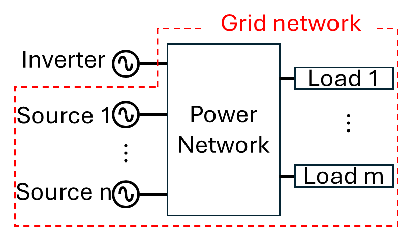
(a) Grid with complex structure

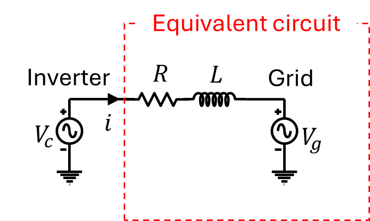
(b) Thevenin equivalent model

Figure 1: Grid model

Let $\overrightarrow{V_{c}}$, $\overrightarrow{V_{g}}$, $\overrightarrow{i}$, and $R$ and $L$ represent the space phasors of the voltage across the inverter’s output capacitance, the grid voltage, the inverter current, and the line impedances, respectively (see Fig. 1). The system dynamics are described by the following equation:

$$\begin{split}\overrightarrow{V_{c}}=R\overrightarrow{i}+L\frac{d\overrightarrow{i}}{dt}+\vec{V_{g}}.\end{split}$$ (1)

If we represent the magnitudes of the grid voltage, the inverter voltage and the output current respectively by $\overline{V_{g}}$, $\overline{V_{c}}$, $\overline{i}$, their phasors in a stationary frame can be expressed as:

$$\begin{split}\overrightarrow{V_{g}}(t)&=\overline{V_{g}}(t)e^{j(\int_{0}^{t}\omega_{grid}(\tau)d\tau+\phi_{grid})}\\ \overrightarrow{V_{c}}(t)&=\overline{V_{c}}(t)e^{j(\int_{0}^{t}\omega_{inv}(\tau)d\tau+\phi_{inv})}\\ \overrightarrow{i}(t)&=\overline{i}(t)e^{j(\int_{0}^{t}\omega_{curr}(\tau)d\tau+\phi_{curr})},\end{split}$$ (2)

where $\omega_{grid}$, $\omega_{inv}$, $\omega_{curr}$ represent the frequency of each signal, ensuring $\phi_{grid}$, $\phi_{inv}$, $\phi_{curr}$ remains constant.

Also, (2) can be rewritten using the rotating frequency $\omega$ as:

$$\begin{split}\overrightarrow{V_{g}}(t)&=\overline{V_{g}}(t)e^{j(\int_{0}^{t}\omega(\tau)d\tau+\psi_{grid}(t))}\\ \overrightarrow{V_{c}}(t)&=\overline{V_{c}}(t)e^{j(\int_{0}^{t}\omega(\tau)d\tau+\psi_{inv}(t))}\\ \overrightarrow{i}(t)&=\overline{i}(t)e^{j(\int_{0}^{t}\omega(\tau)d\tau+\psi_{curr}(t))},\end{split}$$ (3)

where $\psi_{grid}$, $\psi_{inv}$, $\psi_{curr}$ represent the phases of each signal in the rotating frame. Then, the direct-quadrature $(dq)$ components of any phasor $\vec{z}$ in the rotating frame are given by $z_{d}+jz_{q}:=e^{-j\int_{0}^{t}\omega(\tau)d\tau}\vec{z}$. By applying this with (3), (1) can be rewritten as:

$$\begin{split}V_{c}^{d}&=Ri^{d}+L\dot{i^{d}}+\omega Li_{q}+V_{g}^{d}\\ V_{c}^{q}&=Ri^{q}+L\dot{i^{q}}-\omega Li_{d}+V_{g}^{q},\end{split}$$ (4)

where $V_{c}^{d}=\overline{V_{c}}\cos(\psi_{inv})$, $V_{c}^{q}=\overline{V_{c}}\sin(\psi_{inv})$, $V_{g}^{d}=\overline{V_{g}}\cos(\psi_{grid})$, $V_{g}^{q}=\overline{V_{g}}\sin(\psi_{grid})$.

II-B Proposed rotating frame

Estimation of $R$ and $L$ in (4) is much simpler and becomes feasible when the unknown grid voltage $V_{g}^{d,q}$ are constant. However, from (2) and (3), it is evident that the phase of signals in rotating frame is highly dependent on the choice of the frequency $\omega$. By comparing (2) with (3), we get:

$$\begin{split}&\int_{0}^{t}\omega_{grid}(\tau)d\tau+\phi_{grid}=\int_{0}^{t}\omega(\tau)d\tau+\psi_{grid}(t),\\ &\quad\Rightarrow\frac{d}{dt}\psi_{grid}(t)=\omega_{grid}(t)-\omega(t).\end{split}$$ (5)

If grid voltage measurements were available, we could use a PLL to lock the rotating frequency at $\omega_{grid}$ and maintain a constant $\psi_{grid}=\phi_{grid}$. However, since we do not have access to the grid voltage, typical approaches rely on the inverter voltage and its PLL who ensures $\omega=\omega_{inv}$ by driving $\psi_{inv}\rightarrow 0$, or equivalently $V_{c}^{q}\rightarrow 0$. This is done actively through a feedback control law as shown in [12]:

$$\omega(t)=H(p)V_{c}^{q}(t)$$ (6)

where $H(p)$ is a linear transfer function, and $p=\frac{d(\cdot)}{dt}$ represents the differentiation operator.

The primary limitation of this design can be explained as follows. The phase difference $\delta=\psi_{grid}-\psi_{inv}$ represents the phase offset between the grid and inverter voltages. Under the rotating frame of the inverter’s PLL, $\delta=\psi_{grid}$. Since $\delta$ changes with the current injected by the inverter, $V_{g}^{d}$ and $V_{g}^{q}$ are not constant in this rotating frame. This poses a problem because the phase difference $\delta$ and the current $i$ are correlated, and unlike random, uncorrelated errors, this correlation introduces significant estimation errors in line impedance calculations.

We propose design of $\omega$ by analyzing the time-derivatives of $V_{g}^{d}=\overline{V_{g}}\cos(\psi_{grid})$ and $V_{g}^{q}=\overline{V_{g}}\sin(\psi_{grid})$, which are given by

$$\frac{dV_{g}^{d}}{dt} = -\overline{V_{g}}\sin(\psi_{grid})\frac{d\psi_{grid}}{dt}$$ (7)

$$\frac{dV_{g}^{q}}{dt} = \overline{V_{g}}\cos(\psi_{grid})\frac{d\psi_{grid}}{dt};$$ (8)

Here we have assumed that the grid amplitude $\overline{V_{g}}$ is tightly regulated. Therefore a good design of $\omega$ should ensure that both $\frac{d\psi_{grid}}{dt}$ and $\psi_{grid}$ are both small. We analyze each of the these terms below.

In normal operations, when the grid frequency is tightly regulated and changes slowly, we can assume that there are no rapid fluctuations in $\omega_{grid}$. Therefore, as can seen in (5), any fast changes in the rotating frame frequency $\omega$ would contribute to changes in $\frac{d\psi_{grid}}{dt}$, typically occurring when the inverter adjusts its current set point. This motivates us to choose $\omega(t)$ which is band-limited. Therefore by introducing an additional rotating reference frame with a slowly changing frequency—distinct from the inverter’s primary PLL, which has high bandwidth for voltage and current control application—we can effectively reduce the rapid variations in $\psi_{grid}$.

On the other hand in operations with sudden changes in the grid, such as significant load variations, the grid frequency $\omega_{grid}$ can experience large fluctuations, while the inverter’s current tends to change more slowly. This results in gradual (slow) variations in $\psi_{grid}$. Therefore, we need to ensure that our measurements are less sensitive to variations in $\psi_{grid}$. The sensitivity of $V_{g}^{d}$ with respect to changes in $\psi_{grid}$ as seen from (7) is small when $\psi_{grid}$ is small. This can be achieved by ensuring$\psi_{inv}$ small since $\delta$ is typically small, and making $\psi_{inv}$ small will also keep $\psi_{grid}=\psi_{inv}+\delta$ small.

In summary we propose using a secondary PLL with a low bandwidth. With a low bandwidth, we can achieve frequency separation while also preventing $\psi_{inv}$ to be large, as PLL drives the frequency toward $V_{c}^{q}$ to be small.

Note that, while the $d$ and $q$ axis dynamics can separately provide information useful for estimating $R$ and $L$ when $\psi_{grid}$ is fixed, making $\psi_{grid}$ small using a secondary PLL increases the sensitivity of $V_{g}^{q}$ to $\psi_{grid}$. This can cause significant fluctuations in $V_{g}^{q}$, leading to huge errors in the $q$-axis dynamics. Therefore, we proposed using only $d$ axis dynamics for estimation. By isolating the less sensitive $d$ axis dynamics from the more sensitive $q$ axis dynamics, we achieve more robust result and minimize the impact of perturbations on the estimation process.

III Estimation of line parameters: Recursive Least Squares estimation algorithms

In the previous section, we designed the coordinate frame, which attenuated temporal variations of the grid voltage $V_{g}$. We proposed using only the $d$-axis dynamics of (4) , where $V_{g}^{d}$ is not affected much by the effect of phase changes in $V_{g}$. This ensure that the difference $V_{g}^{d}(k+1)-V_{g}^{d}(k)$ is small in successive and close instants $t_{k}$ and $t_{k+1}$; Consequently, for estimating the line parameters $R$ and $L$, we utilize the following difference equation:

$$\begin{split}&\underbrace{V_{c}^{d}(k+1)-V_{c}^{d}(k)}_{y}\\ &=\underbrace{\begin{bmatrix}i^{d}(k+1)-i^{q}(k)\\ \dot{i^{d}}(k+1)-\dot{i^{d}}(k)-\omega(k+1)i^{q}(k+1)+(k)i^{q}(k)\end{bmatrix}^{\top}}_{u^{\top}}\underbrace{\begin{bmatrix}R\\ L\end{bmatrix}}_{\theta}\\ &\quad+\underbrace{V_{g}^{d}(k+1)-V_{g}^{d}(k)}_{w}.\end{split}$$ (9)

Here the output and input vectors $y(k)$ and $u(k)$ are data obtained from local measurements at the inverter. The vector $\theta$ represents the line parameters to be estimated, while $w$ captures the noise associated with variations in the grid voltage. Since we are estimating only two parameters using the RLS algorithm, the computations are significantly faster, reducing $3\times 3$ matrix operations to $2\times 2$. Once the estimations $\widehat{R}$, $\widehat{L}$ are acquired, the grid voltage estimation $\widehat{V_{g}^{d}}$ and $\widehat{V_{g}^{q}}$ can be acquired by substituting the estimated values in (4). The objective of estimation problem is to find an optimal (in the least square sense) $\widehat{\theta}$ that satisfies $y=u^{\top}\widehat{\theta}$.

III-A RLS and CF-RLS

We introduce the RLS and CF-RLS algorithms, previously applied in line-parameter estimation [10, 4]. Our proposed method builds on these algorithms, so we first explain them to highlight their limitations and how our approach of using VDF-RLS, addresses these shortcomings. In the RLS and CF-RLS algorithms, an optimal estimate $\widehat{\theta}_{K}$ is obtained at each $K$th measurement instant by minimizing the following cost function:

$$J(\widehat{\theta},K)=\sum_{k=1}^{K}\lambda^{K-k}\left(y(k)-u^{\top}(k)\widehat{\theta}\right)^{\top}\left(y(k)-u^{\top}(k)\widehat{\theta}\right),$$ (10)

where $\lambda\in(0,1]$ is the forgetting factor. If $\lambda=1$, it is the regular RLS algorithm, where there is no forgetting; that is, the data set from the entire time horizon $1\cdots K$ is weighted equally—from the beginning of the algorithm to the most recent data. On the other hand, in CF-RLS, where a constant forgetting factor $0<\lambda<1$ is chosen, more weight is given to the most recent data. As $\lambda$ decreases, it prioritizes recent data, helping the estimation converge to new parameters when changes occur. Conversely, if $\lambda$ is large, it minimizes the influence of noise or errors, preventing fluctuations in the estimation

The optimal $\widehat{\theta}_{K}$ obtained from $\frac{\partial J}{\partial\widehat{\theta}}=0$ is given by:

$$\widehat{\theta}_{K} =\bigg{(}\sum_{k=1}^{K}\lambda^{K-k}u(k)u^{\top}(k)\bigg{)}^{-1}\bigg{(}\sum_{k=1}^{K}\lambda^{K-k}u(k)y(k)\bigg{)}.$$ (11)

This can be expressed in recursive form as:

$$\begin{split}\hat{\theta}_{K}&=\hat{\theta}_{K-1}+R_{K}^{-1}u(K)\big{(}y(K)-u^{\top}(K)\hat{\theta}_{K-1}\big{)}.\\ \end{split}$$ (12)

Here, $R_{K}$ is the information matrix, which can be updated recursively as:

$$R_{K}=\bigg{(}\sum_{k=1}^{K}\lambda^{K-k}u(k)u^{\top}(k)\bigg{)}=(\lambda R_{K-1}+u(K)u^{\top}(K)).$$ (13)

With this recursive form, there is no need to store all the data; only the information matrix and the previous estimate are required to update the new estimate when a new measurement is obtained. Note that implementing equation (12) requires calculating matrix inversion. This can be further expressed recursively using the matrix inversion lemma. However, since $R_{K}$ is a $2\times 2$ matrix in our estimation problem, we will not explore this further due to its manageable size.

The main challenge in estimation arises from the lack of sufficiently rich data that does not persist over time. This leads to information matrices that are either non-invertible or have very large condition numbers. The CF-RLS algorithm introduces a tradeoff: small values of $\lambda$ discard past information, placing more weight on new data, while larger values of $\lambda$ retain more past information, reducing the relative importance of recent data. Information matrices tend to have good condition numbers (and are invertible) if the available data is sufficiently rich within a short time frame. For example, for any small $\epsilon>0$, the information matrix effectively incorporates data from the past $K=\frac{\log\epsilon}{\log\lambda}$ measurements, as $\lambda^{K}\leq\epsilon$ beyond this time horizon. If there is insufficient new information in $u(k)$ within this period, $R_{K}$ will either become non-invertible or have a high condition number. As shown in equation (13), this method forgets the entire previous information matrix, regardless of the quality of the new data.

In the context of power systems, it is common for the data to lack sufficient richness within such short intervals of time. For example, an inverter might maintain a constant current, meaning $u\approx 0$ over long periods, with only occasional set-point changes. In such scenarios, there is insufficient data richness for the information matrix to remain invertible within the time intervals dictated by a reasonable forgetting factor $\lambda$. In fact, during extended periods of constant current, the information matrix exponentially converges to the zero matrix. More generally, with CF-RLS, if there is no persistent excitation—where the $2\times 1$ input vector $u(t)$ lies along a single direction within the effective time horizon—the smaller singular value of $R_{K}$ will exponentially decay to zero at a rate determined by $\lambda$, except in the direction of $u$. Consequently, the singular value of $R_{K}^{-1}$ grows exponentially, making the estimation highly sensitive to that particular direction, as $R_{K}^{-1}$ dictates the update of the estimate, as seen in equation (12).

III-B VDF-RLS

Therefore, to address the issue of insufficient data richness over short time intervals, we apply the VDF-RLS algorithm. In this method, the forgetting factor is applied selectively, targeting only the portion of the information matrix that corresponds to the new input vector $u$. This involves first evaluating the singular vectors of the information matrix, where the singular values associated with these vectors quantify the amount of information in their respective directions. Zero or low singular values indicate a lack of information richness in those directions. More specifically, we represent the singular value decomposition of information matrix as:

$$R_{K}=V_{K}\Sigma_{K}V_{K}^{\top}=\sum_{i}\sigma_{i,K}v(i,K)v^{\top}(i,K),$$ (14)

where $\sigma_{i,K}$ and $v(i,K)$ correspond to a $i$th singular value and singular vector of information matrix $R_{K}$ at $K$th time instance. An input vector at the next instance $u(K+1)$ can then be evaluated as to how much it is aligned with $v(i,K)$ ; here the alignment is by evaluate by the inner product $u(K+1)^{\top}v(i,K)$. The forgetting factor for eacht direction is then ascribed as:

$$\lambda_{i}=\begin{cases}\lambda\in(0,1)\quad(\text{if }|v(i,K)^{\top}u(K+1)|>\text{threshold})\\ 1\quad\text{else}\end{cases}$$ (15)

In this approach, the forgetting factor is applied only when the inner product between the new input vector and the singular vectors exceeds a certain threshold. By adjusting this threshold, we can enhance the algorithm’s robustness against noise. Specifically, when the magnitude of the input vector is small, it is treated as noise; even if the angle between the input vector and the information direction is aligned, the forgetting factor is not applied in such cases.

With the forgetting factor defined in (15), the information matrix can be updated as follows:

$$\begin{split}R_{K+1}&=\sum_{i}\lambda_{i}\sigma_{i,K}v(i,K)v^{\top}(i,K)+u(K+1)u^{\top}(K+1)\\ &=V_{K}\sqrt{\Lambda}\Sigma_{K}\sqrt{\Lambda}V_{K}^{\top}+u(K+1)u^{\top}(K+1).\end{split}$$ (16)

where $\Lambda$ is a diagonal matrix whose $i$ th diagonal element is $\lambda_{i}$. Then, the new estimation can be obtained recursively using (12).

Note that the recursion in (12) requires $R_{K}$ to be invertible. Therefore, before the recursive form can be applied, the algorithm must wait until sufficient data is collected to ensure that $R_{K}$ becomes invertible. However, for the CF-RLS with $\lambda\in(0,1)$ and VDF-RLS, regardless of the starting values $R_{0}$ and $\widehat{\theta}_{0}$, the algorithm will eventually converges to the desired $\widehat{\theta}_{K}$, as initial conditions are gradually forgotten with enough excitation. This allows for simpler implementation, allowing the algorithm to start from any invertible matrix $R_{0}$ and an initial guess $\widehat{\theta}_{0}$.

IV Simulation results

Figure 2: Simulation setup

The proposed impedance estimation algorithm was implemented and tested using the MATLAB Simscape toolbox with a step size of 0.05 ms. As illustrated in Fig. 2, the simulation models an inverter connected to the grid with a voltage of $480,V_{\text{rms L-L}}$ and a frequency of 59.95 Hz, through a variable impedance. The inverter operates in grid-following mode, adjusting its output to meet a specified power set point. The initial conditions for the parameter estimation and the information matrix are set as $\widehat{\theta}_{0}=[0,0]^{\top}$ and $R_{0}=0.001I_{2}$.

IV-A Evaluation on proposed reference frame

IV-A1 The source of rotating frame

Here, we compare the rotating reference frames used in prevailing designs for rotating frequencies $\omega$ with our proposed design. Specifically, we examine the rotational frequencies determined by the primary PLL design, the nominal $60\text{Hz}$, frequency obtained by low-pass filtering of primary PLL frequencies, and those from our secondary PLL design (See Fig. 3). In all simulations, the grid frequency is set to $59.95$ Hz, while the nominal frequency is $60$ Hz. To evaluate the effect of the selected rotating frame and the impact of the phase difference $\delta$ between the grid and the inverter within the rotating frame, we introduce persistent excitation by setting the active power setpoint to $10+2\sin(20t)$ kW and the reactive power setpoint to $2\sin(30t)$ kVAR. Under all conditions, the VDF-RLS algorithm, using only the $d$-axis dynamic, is applied with a constant forgetting factor ($\gamma=0.99$) and threshold value ($0.02$).

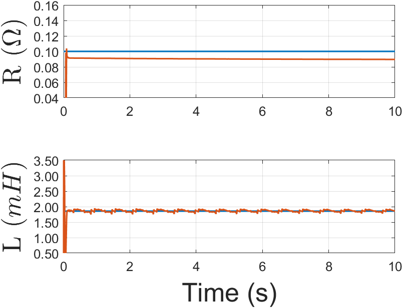
(a)

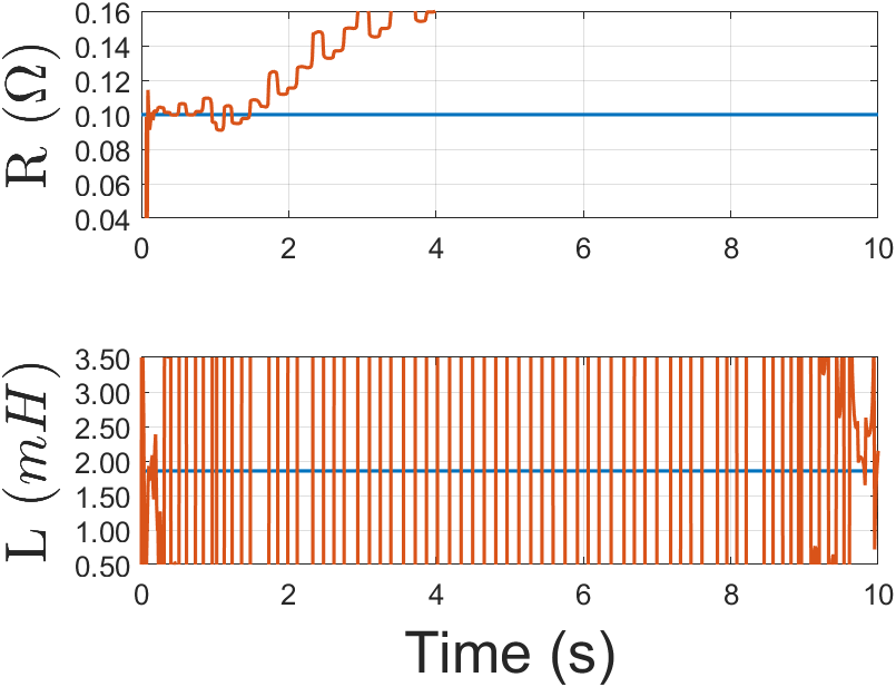
(b)

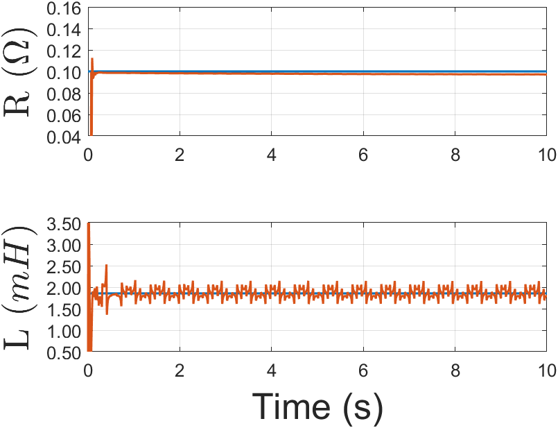
(c)

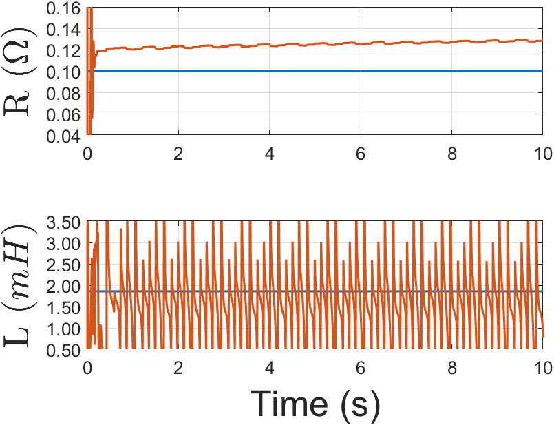
(d)

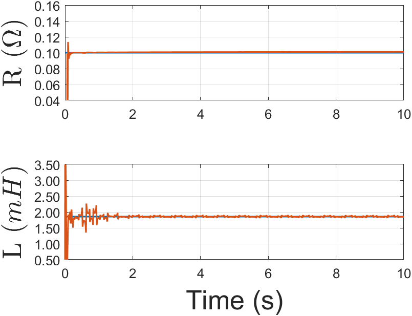
(e)

Figure 3: Estimation result using the rotating frame given by (a) The frequency provided by the inverter’s primary PLL (b) The nominal grid frequency(60Hz) (c) A low-pass filtered version of the inverter’s primary PLL frequency with a cutoff frequency of 5 rad/s and an initial phase of $\psi_{inv}(0)=0$ (d) A low-pass filtered version of the inverter’s primary PLL frequency with a cutoff frequency of 5 rad/s and an initial phase of $\psi_{inv}(0)=\pi/4$ (e) The frequency given by our secondary PLL with a bandwidth 5rad/s

The estimation performance is evaluated by the Root Mean Square Percent Error (RMSPE) for each parameter (see Table I), where

$$\begin{split}RMSPE=\sqrt{\frac{1}{N}\sum_{k=1}^{N}\bigg{(}\frac{\widehat{\theta}_{i}(k)-\theta_{i}(k)}{\theta_{i}(k)}\bigg{)}}\times 100\%.\end{split}$$ (17)

Here, due to a significant initial transient that impacts the RMSPE, the evaluation for each RMSPE begins $1$ second after the scenario starts.

TABLE I: RMSPE of R and L estimation under different rotating frame

Rotating frame frequency source	RMSPE R (%)	RMSPE L(%)
Primray PLL freq	9.7795	1.8251
Nominal Frequency	90.9519	548.0205
LPF of Primary PLL freq	2.3030	5.4050
with initial condition $\psi_{inv}(0)=0$
LPF of Primary PLLfreq	25.2924	66.7926
with initial condition $\psi_{inv}(0)=\pi/4$
2nd PLL freq	0.8891	1.0890
2nd PLL freq	18.1615	19.0683
using both $d$ and $q$ dynamics

With the inverter’s primary PLL, which has a fast bandwidth, the estimated parameters converge to a certain value and do not fluctuate significantly. However, as shown in Fig. 3 (a), the parameters do not align to the actual values of $R$ and $L$. This discrepancy occurs because, while the primary PLL maintains $\psi_{inv}=0$, the excitation-induced variations in $\delta$ introduce errors into the estimation process.

In [10], when the grid frequency matches the nominal frequency, the system ensures that $V_{g}^{d}$ and $V_{g}^{q}$ remain constant, resulting in accurate estimation. However, when the grid frequency deviates from its nominal value, $V_{g}^{d}$ and $V_{g}^{q}$ continually change under this rotating frame, which becomes a significant source of error in the estimation. As illustrated in Fig. 3 (b), the algorithm does not converge under these conditions.

Using the low-pass filtered frequency from the inverter’s primary PLL mitigates the impact of perturbations in $\delta$ as demonstrated in Fig. 3 (c). However, this approach does not ensure where $\psi_{inv}$ is; different initial values of $\psi_{inv}(0)$ can yield varying results. Fig. 3 (d) illustrates this scenario with different initial conditions for $\psi_{inv}$, where the estimation results show significant error. This highlights that the low-pass filter alone does not guarantee uniform performance.

Finally, as seen in Fig. 3 (e),the proposed approach using a secondary PLL combines the benefits of both the low-pass filter and the primary PLL. It achieves low error while ensuring consistent performance by rejecting changes in $\delta$ through the use of a low bandwidth and reducing sensitivity to $\delta$ variations by keeping $\theta_{inv}$ small. This dual approach improves the stability and accuracy of the impedance estimation under varying grid conditions.

IV-A2 Sensitivity to $d$ and $q$ axis grid voltage error

Then, using the rotating frame provided by the secondary PLL, we consider the case where both $d$ and $q$ axis dynamics are utilized. Due to the change in dimensions, we define the output as $y=\begin{bmatrix}\Delta V_{c}^{d}\\ \Delta V_{c}^{q}\end{bmatrix}$ and the input vector as $u=\begin{bmatrix}\Delta i^{d}&\Delta(\dot{i^{d}}-\omega i^{q})\\ \Delta i^{q}&\Delta(\dot{i^{q}}+\omega i^{d})\end{bmatrix}$. Additionally, during the update process, we evaluate the alignment of the input vector using $\|v(i,K)^{\top}u(K+1)\|_{2}$ instead of the absolute value to accommodate the dimensional changes.

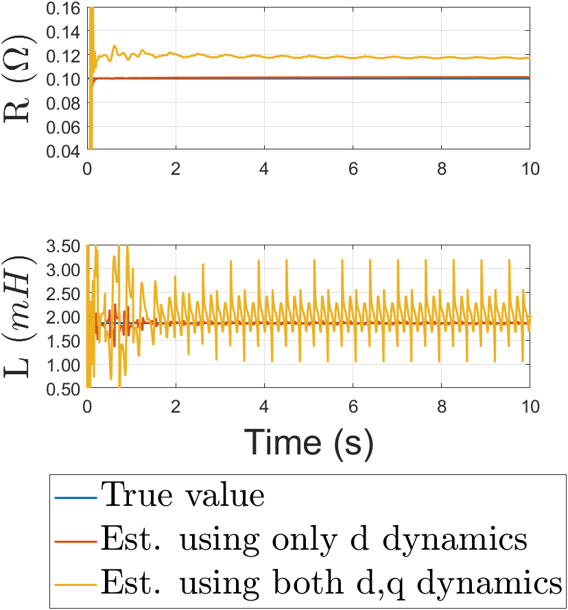
(a)

(b)

Figure 4: (a) Estimation result comparison between using only d axis and both d,q axis dynamics (b) $d$, $q$ component grid voltage and error from them

As seen in Fig. 4 (a), when both $d$ and $q$ axis dynamics are used, the estimation results shows large fluctuations and higher RMSPE values (see Table I) compared to the scenario where only $d$ axis dynamics are used, despite the additional information provided by the $q$ axis dynamics.

This fluctuation arises from noise. When using both $d$ and $q$ axis dynamics, the noise is given by $w=\begin{bmatrix}\Delta V_{c}^{g}\\ \Delta V_{c}^{g}\end{bmatrix}$. Even within the same reference frame, $V_{g}^{q}$ experience larger fluctuation, leading to larger $\Delta V_{g}^{q}$ compare to $V_{g}^{d}$ and $\Delta V_{g}^{d}$ as shown Fig. 4 (b). This is due to its larger sensitivity as discussed in previous section. In contrast, using only $d$ axis dynamics allows for effective rejection of this noise.

IV-B Performance comparison between VDF-RLS and CF-RLS

IV-B1 With Persistent Excitation

To compare the estimation performance between the VDF-RLS algorithm and the CF-RLS algorithm, we evaluated the CF-RLS algorithm under the same excitation signal as before. Also, the line impedance $R$ and $L$ is changed at $t=5$s.

As shown in Fig. 5 (a), both CF-RLS and VDF-RLS algorithm show approaches to true value initially, and update its estimation right after impedance change occurs. However, the CF-RLS algorithm exhibits greater fluctuations in estimation, resulting in larger errors. Their RMSPE values for $R$ and $L$ estimations are 0.6917% and 1.3240% using VDF-RLS, compared to 8.1011% and 1.7646% using CF-RLS before impedance changes (evaluated $1\leq t\leq 5$s). After the impedance changes (evaluated $1\leq t\leq 5$s), their RMSPE values for $R$ and $L$ estimations are 3.5078% and 8.3129% using VDF-RLS, versus 56.3065% and 36.6484% using CF-RLS before impedance changes (evaluated $6\leq t\leq 10$s). This instability arises from the forgetting mechanism, which in the CF-RLS algorithm is applied uniformly across all directions. In contrast, the VDF-RLS algorithm applies forgetting selectively to certain directions, enhancing robustness against noise by incorporating a defined threshold. Consequently, as illustrated in Fig. 5 (b), while the first singular values of both algorithms are nearly identical, the second singular value for the CF-RLS algorithm is significantly smaller. This reduced second singular value increases the sensitivity of the estimation algorithm to noise.

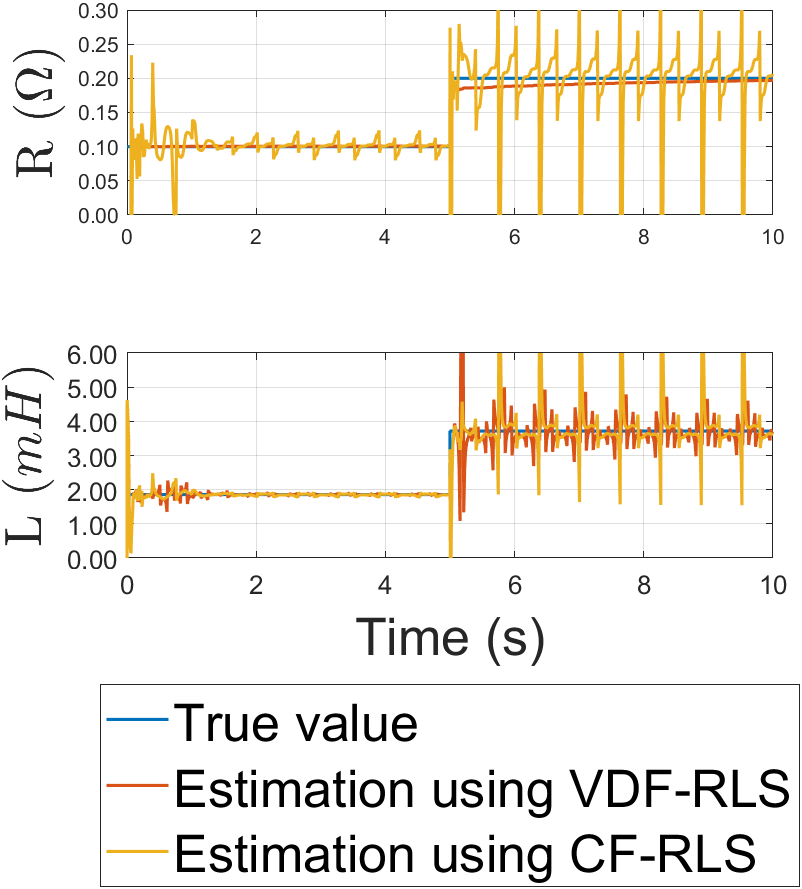
(a)

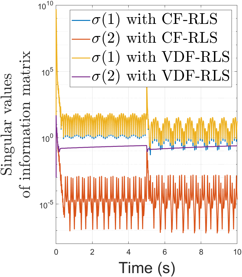
(b)

Figure 5: Performance comparison between VDF-RLS and CF-RLS under persistent excitation. (a) $R$, $L$ estimation result (b) singular values of information matrix

IV-B2 Without Persistent Excitation

Consider the scenario where the inverter’s setpoints for active and reactive power, $P_{0}$ and $Q_{0}$, are changing int a step manner; Initially, $P_{0}=7.5kW$ and $Q_{0}=0kVAR$; at $t=2.5$s, $P_{0}=10kW$ and $Q_{0}=2kVAR$; at $t=7.5$s $P_{0}=11kW$ and $Q_{0}=2kVAR$; and finally at $t=12.5$s $P_{0}=8kW$ and $Q_{0}=1kVAR$. Also, there are changes in impedance occur at $t=5$s and $t=10$s. The parameter estimation results are presented in Fig. 6 (a).

Initially, as there is no excitation, VDF-RLS maintains the initial condition. However, once the step changes in current is applied at $t=2.5$s, estimation result updated and converge toward the desired $R$ and $L$ values. Moreover, when the impedance changes at $t=5$s, the excitation induced by the impedance changes facilitates convergence to the desired values. While there is some estimation error, estimation update due to excitation at $t=7.5$s further reduces this error. A similar pattern occurs at $t=10$s and $t=12.5$s, where impedance changes and step changes in the operating point are again applied.

However, with the CF-RLS algorithm using $\lambda=0.99$, when there is no excitation, the information matrix approaches singularity, causing significant fluctuations in the estimation results. To address this issue, comparisons were made with scenarios where $\lambda=0.999$ and $\lambda=0.9999$ were used instead.

While the $R$ and $L$ estimation approaches to the desired values when excitation is given, the singular values of information matrix diminish when there is no excitation as seen in Fig. 6 (b). This increased sensitivity to noise causes the estimation results to drifting of estimation result, as seen in Fig. 6 (a) CF-RLS case with $\lambda=0.999$ around $t=3$s, $t=6$s, $t=8$s, $t=11$s, and $t=13$s.

The drifting issue can be mitigated by selecting a larger $\lambda$. As shown in Fig. 6 (a), in the case with $\lambda=0.9999$, a larger $\lambda$ reduces the drift in the estimation. However, even with the larger $\lambda$, without persistent excitation, as seen in Fig. 6 (b), the algorithm gradually lose information, leading to drift eventually. Furthermore, using a higher $\lambda$ values prevents the algorithm from tracking changes in $R$ and $L$ when their value is change, requiring additional excitation to properly track parameters.

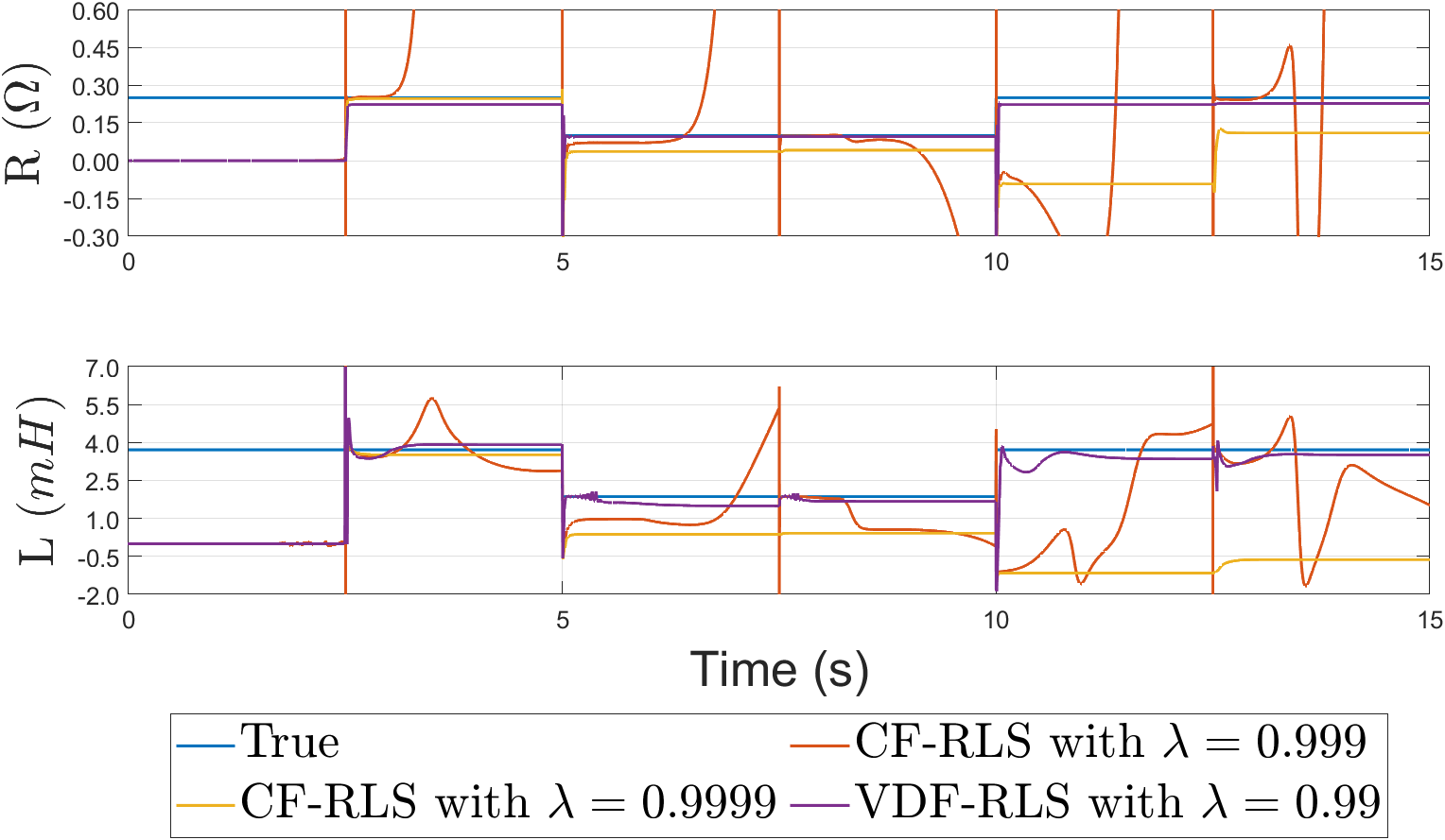
(a) Impedance estimation using CF-RLS and VDF-RLS method

(b) Singular values of imformation matrix

Figure 6: Comparison between VDF-RLS and CF-RLS without persistent excitation

V CONCLUSIONS

In this paper, we propose a VDF-RLS-based grid line parameter estimation algorithm operating within a secondary PLL-based rotating frame. To accurately estimate the line parameters, it is crucial to separate the effects of the grid voltage from the inverter dynamics. We argue that employing a PLL with an appropriately chosen bandwidth can effectively isolate the grid voltage while minimizing sensitivity to perturbations caused by the inverter’s operation. Additionally, with the VDF-RLS algorithm, as the history of information is selectively updated when new data is acquired, the method remains stable even in the absence of persistent excitation, and it effectively estimates the parameter when excitation is given.

We demonstrate this through simulations, comparing the parameter estimation results using data from various rotating frames. Additionally, we compare the VDF-RLS algorithm with the CF-RLS algorithm, evaluating their performance both with and without persistent excitation conditions.

References

- [1] T. Hossen, F. Sadeque, M. Gursoy, and B. Mirafzal, “Self-secure inverters against malicious setpoints,” in 2020 IEEE Electric Power and Energy Conference (EPEC). IEEE, 2020, pp. 1–6.
- [2] Q.-C. Zhong and Y. Zeng, “Universal droop control of inverters with different types of output impedance,” IEEE access, vol. 4, pp. 702–712, 2016.
- [3] A. Askarian, J. Park, and S. Salapaka, “Enhanced grid following inverter (e-gfl): A unified control framework for stiff and weak grids,” IEEE Transactions on Power Electronics, pp. 1–17, 2024.
- [4] I. Jarraya, J. Hmad, H. Trabelsi, A. Houari, and M. Machmoum, “An online grid impedance estimation using recursive least square for islanding detection,” in 2019 16th International Multi-Conference on Systems, Signals & Devices (SSD). IEEE, 2019, pp. 193–200.
- [5] J. Park, A. Askarian, and S. Salapaka, “Control designs for critical-continegency responsible grid-following inverters and seamless transitions to and from grid-forming modes,” in 2024 American Control Conference (ACC), 2024, pp. 2958–2963.
- [6] W. Jiang and H. Tang, “Distribution line parameter estimation considering dynamic operating states with a probabilistic graphical model,” International Journal of Electrical Power & Energy Systems, vol. 121, p. 106133, 2020.
- [7] M. Ciobotaru, R. Teodorescu, and F. Blaabjerg, “On-line grid impedance estimation based on harmonic injection for grid-connected pv inverter,” in 2007 IEEE international symposium on industrial electronics. IEEE, 2007, pp. 2437–2442.
- [8] A. Ghanem, M. Rashed, M. Sumner, M. A. Elsayes, and I. I. Mansy, “Grid impedance estimation for islanding detection and adaptive control of converters,” IET Power Electronics, vol. 10, no. 11, pp. 1279–1288, 2017.
- [9] J. C. Vasquez, J. M. Guerrero, A. Luna, P. Rodríguez, and R. Teodorescu, “Adaptive droop control applied to voltage-source inverters operating in grid-connected and islanded modes,” IEEE transactions on industrial electronics, vol. 56, no. 10, pp. 4088–4096, 2009.
- [10] S. Cobreces, P. Rodriguez, D. Pizarro, F. Rodriguez, and E. Bueno, “Complex-space recursive least squares power system identification,” in 2007 IEEE Power Electronics Specialists Conference. IEEE, 2007, pp. 2478–2484.
- [11] A. Goel, A. L. Bruce, and D. S. Bernstein, “Recursive least squares with variable-direction forgetting: Compensating for the loss of persistency [lecture notes],” IEEE Control Systems Magazine, vol. 40, no. 4, pp. 80–102, 2020.
- [12] A. Yazdani and R. Iravani, Voltage-sourced converters in power systems: modeling, control, and applications. John Wiley & Sons, 2010.