Digesting Gibbs Sampling Using R

Dedicated to my parents.

Preface

This work aims to provide an environment for all users who are beginner in the context of the statistical simulation approaches. These techniques are known as the Monte Carlo methods as a whole nowadays. Indeed, the Monte Carlo, as a statistical simulation technique, itself involves the Markov chain Monte Carlo that attracts the attention of researchers from a wide variety of study fields. One may see the Markov chain Monte Carlo as statistical simulation approaches that work based on the iterative algorithms and so the others that are not based on iterative algorithm are the Monte Carlo approaches. We would recommend the reader(s) to learn the elementary undergraduate courses in calculus, probability, and statistics before studying or applying this report for practical purposes. The required topics may include, but not limited to, concept of mathematical function, limit, derivative, partial derivative, simple integrals, probability axioms, discrete and continuous random variables, probability distributions, concept of central tendency and variance, multivariate probability distributions, functions of random variables, and the central limit theorem (CLT). There is no doubt that almost all of researchers are using statistical methods for supporting their finding(s). When the sample evidence are summarized in a quantity that is called statistic, then statistical decision is made by comparing the computed statistic with some criterion or critical value, leading to accepted or reject the relevant question (hypothesis). Sometimes sample evidence are not gathered from field work and the process of sampling must be implemented within a statistical laboratory that is known as statistical simulation. In fact, sample evidence are simulated (or generated) artificially by researcher through the Monte Carlo methods. The process of simulation is carried out for some specific purposes including computing the reliability of systems or devices in engineering, estimation of benefit, computing the standard error of an statistical estimation, etc. Hence, the terms such as “A limited Monte Carlo study was carried out to demonstrate$\cdots$”, “We carried out a Monte Carlo study to $\cdots$”, and similar expressions may be seen in many scientific reports and monographs. But, the Markov Chain Monte Carlo techniques seem to comprise the large part of the Monte Carlo methods. So, the main concern of this report is placed on showing how users can apply the Markov Chain Monte Carlo techniques in practice. Almost all of examples are followed by the corresponding R codes in order to better understand the theoretical topics in the context of probability and statistics. Hence, overall knowledge of a statistical software R is essential.

Acknowledgements

• Special thanks goe to Amber Jain for a free-to-edit LaTeX template for book-style compilations that is available at https://github.com/amberj/latex-book-template/blob/master/book-template.tex#L29.

• I’m deeply indebted my parents and friends for their support and encouragement.

Mahdi Teimouri Yanesari,
Assistant Professor in Statistics,
Department of Statistics,
Gonbad Kavous University, Iran.
Email:  mahdiba_2001@yahoo.com

Chapter 1 Metropolis-Hastings algorithm

“Be approximately right rather than exactly wrong.”

– John W. Tukey, June 16, 1915 - July 26, 2000

1.1 Metropolis-Hastings algorithm

Herein, we give a general description of the Metropolis-Hastings algorithm followed by one illustration implemented in R environment. First, we recall three basic definitions as follows.

Definition 1.1.1.

A collection of sample evidence (random variables) indexed by time set $t\in\mathbb{N}$, represented as $\bigl{\{}X_{t}\big{\}}_{t\in\mathbb{N}}$, is called stochastic or random process.

Definition 1.1.2.

A stochastic (or random) process $\bigl{\{}X_{t}\big{\}}_{t\geq\mathbb{N}}$ follows a Markov property or Markov process if

$$p\bigl{(}X_{n}=x_{n}\big{|}X_{1}=x_{1},\cdots,X_{n-1}=x_{n-1}\bigr{)}=p\bigl{(}X_{n}=x_{n}\big{|}X_{n-1}=x_{n-1}\bigr{)},$$ (1.1)

that means the position (or state) of a Markov process at time $n$ just depends on its position at previous state $n-1$.

Definition 1.1.3.

State $j$ is said to be accessible from a state $i$ (represented by $i\rightarrow j$), if there exists some $n\geq 1$ such that $p^{n}_{ij}=P\bigl{(}X_{n}=j\big{|}X_{0}=i\bigr{)}>0$. This means that we can move from the state $i$ to state $j$ in $n$ steps with probability $p^{n}_{ij}$. If both of $i\rightarrow j$ and $j\rightarrow i$ hold, then states $i$ and $j$ communicate with each other (represented by $i\leftrightarrow j$). Hence, the Markov chain is irreducible if each two states communicate.

As a method with long history invented at the middle of twentieth century (Hitchcock, 2003), the Metropolis ${\cal{S}}_{f}$.

To this end, we constitute a irreducible Markov process (chain) that converges to a stationary (limiting) distribution with PDF $f(\cdot|\theta)$ from which we would like to draw sample. The Metropolis algorithm works by generating sequence $\{x_{1},x_{2},\cdots,x_{n}\}$ from a Markov chain that we expect $x_{n}$ comes from $f(\cdot|\theta)$ for $n\rightarrow\infty$. More precisely, suppose the current state of Markov chain is $x_{n}$, then within a Metropolis algorithm framework, for moving form the current state (generation) $x_{n}$ to the next state (generation) $x_{n+1}$, the transition probability $p\bigl{(}x_{n},x_{n+1}\bigr{)}$, is

$$p\bigl{(}x_{n}\rightarrow x_{n+1}\bigr{)}=\min\left\{1,\frac{f\bigl{(}x_{n+1}\big{|}\theta\bigr{)}l\bigl{(}x_{n}\big{|}x_{n+1}\bigr{)}}{f\bigl{(}x_{n}\big{|}\theta\bigr{)}l\bigl{(}x_{n+1}\big{|}x_{n}\bigr{)}}\right\}.$$ (1.2)

As it is seen, the transition probability depends on the so-called proposal (or candidate) distribution with PDF $l(\cdot|\cdot)$ that is chosen arbitrarily, but symmetric and provided that ${\cal{S}}_{l}={\cal{S}}_{f}$. Notice that the next state $x_{n+1}$ of $l(\cdot|\cdot)$ depends on the current state $x_{n}$, that is $l\bigl{(}x_{n+1}\big{|}x_{n}\bigr{)}$. In practice, for the proposal distribution, the current state can be its mean (or median) and so $l\bigl{(}x_{n+1}\big{|}x_{n}\bigr{)}$ can be interpreted as the chance of moving to the next state $x_{n+1}$ given that the current state on the average is $x_{n}$. For example, if we chose a Gaussian distribution as the proposal whose PDF is represented as ${\cal{N}}\bigl{(}.|\mu,\sigma^{2}\bigr{)}$, then we can write

$$l\bigl{(}x_{n+1}\big{|}x_{n}\bigr{)}={\cal{N}}\bigl{(}x_{n+1}\big{|}\mu=x_{n},\sigma^{2}\bigr{)}.$$

Since moving to next state $x_{n+1}$ depends on the current state $x_{n}$, hence the sequence of the generated samples constitutes a correlated stochastic process. But, despite existence such dependency, the simulated generations are approximately distributed as $f(\cdot|\theta)$. This dependency has its origin from the Markovian nature of the simulation so that the next generation is highly depends on the current state (generation). Usually a set of the initial generations are removed from the whole generated sample as burn-in or warm-up (Robert et al., 2004). While there some criteria to determine when the chain attains its stationary distribution (Hobert and Robert, 2004). It is known that after sufficiently large number $N$ of generations, the generated samples are statistically uncorrelated and converge to the target distribution with PDF $f(.|\theta)$. We follow the steps of Algorithm 1 given by the following for implementing the MH algorithm.

Algorithm 1 MH-algorithm

1:Set $k=0$, read ${{K}}$, and choose the current state (initial generation) $x_{0}$;

2:while $k\leq{{K}}$ do

3:     Sample $x_{k+1}$ from the proposal distribution with PDF $l\bigl{(}\cdot\big{|}x_{k}\bigr{)}$;

4:     Compute

$$p\bigl{(}x_{k}\rightarrow x_{k+1}\bigr{)}=\min\left\{1,\frac{f\bigl{(}x_{k+1}\big{|}\theta\bigr{)}l\bigl{(}x_{k}\big{|}x_{k+1}\bigr{)}}{f\bigl{(}x_{k}\big{|}\theta\bigr{)}l\bigl{(}x_{k+1}\big{|}x_{k}\bigr{)}}\right\}.$$

5:     Generate $u$ from Unif(0, 1);

6:     if $u<p\bigl{(}x_{k},x_{k+1}\bigr{)}$ then

7:         Set $y\leftarrow x_{k+1}$, $k\leftarrow k+1$, and $x_{k}\leftarrow y$;

8:     else

9:         $x_{k+1}\leftarrow x_{k}$ and $k\leftarrow k+1$;      

10:     end

11:end

12:Accept $x_{{K}}$ as a generation form target distribution $f$.

As mentioned above, within a Metropolis algorithm the proposal has a symmetric PDF that is easy to sampling from. That is $l\bigl{(}x_{n+1}|x_{n}\bigr{)}=l\bigl{(}x_{n}|x_{n+1}\bigr{)}$. For example, if we choose $l\bigl{(}x_{n+1}|x_{n}\bigr{)}={\cal{N}}(x_{n+1}|\mu=x_{n},\sigma^{2})$ as the proposal, then the transition probability simplifies to $p\bigl{(}x_{n},x_{n+1}\bigr{)}=\min\{1,f\bigl{(}x_{n+1}|\theta\bigr{)}/f\bigl{(}x_{n}|\theta\bigr{)}\}$. This holds also if the proposal is an uniform distribution on $(\mu-3\sigma,\mu+3\sigma)$ as the proposal for which we have $l\bigl{(}x_{n+1}|x_{n}\bigr{)}=l\bigl{(}x_{n}|x_{n+1}\bigr{)}=1/(6\sigma)$. The algorithm proposed by Metropolis et al. (1953) was then developed by Hastings (1970) for general case in which the proposal can be either symmetric or asymmetric ($l(x_{n+1}|x_{n})\neq l(x_{n+1}|x_{n})$). Today the latter case is known as the Metropolis-Hasting (MH) algorithm. A privilege of the MH algorithm is its capability to apply for the cases that the target distribution needs only to be specified up to proportionality constant. The care must taking into account that target PDF must never be zero at the initial state $x_{0}$ and the candidate $l(\cdot|\cdot)$ must have a broad enough support to visit any state of ${\cal{S}}_{f}$ with a positive probability while gets as simple as possible form. We give more details on finding a suitable proposal through the following example.

Example 1 Let $f(x|\theta)\propto(x+1)^{-2}x^{\theta}\exp\{-x^{\theta}\}$ where $x>0$ and $\theta>0$ is the family parameter. For simulating from target distribution with PDF $f(x|\theta)$, we chose ${\cal{W}}(\cdot|\theta,1)$ as the proposal PDF where ${\cal{W}}(\cdot|\theta,1)$ denotes the PDF of Weibull distribution with shape parameter $\theta$ and scale unity. We write out the transition probability as

$$p\bigl{(}x_{n},x_{n+1}\bigr{)}= \min\left\{1,\frac{(x_{n+1}+1)^{-2}x_{n+1}^{\theta}\exp\{-x_{n+1}^{\theta}\}{\cal{W}}(x_{n}|\beta,1)}{(x_{n}+1)^{-2}x_{n}^{\theta}\exp\{-x_{n}^{\theta}\}{\cal{W}}(x_{n+1}|\beta,1)}\right\}.$$

$$= \min\left\{1,\frac{(x_{n}+1)^{2}x_{n+1}}{(x_{n+1}+1)^{2}x_{n}}\right\}.$$ (1.3)

Fortunately, though using an asymmetric proposal, but transition probability takes a simple form with possibility of taking large values leading to an almost surely transition from $x_{n}$ to $x_{n+1}$. We adopt algorithm given by the following for simulating from $f(x|\theta=5)$.

• Set $k=0$, ${{K}}=1000$, and the initial state (generation) $x_{0}=1$;

  1. Generate $x_{k+1}\sim{\cal{W}}(\theta=5,1)$

  2. Compute $p\bigl{(}x_{k},x_{k+1}\bigr{)}=\min\left\{1,\frac{(x_{k}+1)^{2}x_{k+1}}{(x_{k+1}+1)^{2}x_{k}}\right\}$;

  3. Generate $u\sim{\text{Unif}}(0,1)$;

  4. If $u<p\bigl{(}x_{k},x_{k+1}\bigr{)}$ then $x_{n}\rightarrow x_{k+1}$ (chain moves from state $x_{k}$ to state $x_{k+1}$) and $k\rightarrow k+1$;

  5. Repeat algorithm from step 1;

• Stop algorithm if $k=K$ and then accept $x_{K}$ as a generation from ${\cal{W}}(\theta=5,1)$.

The R code, for generating from PDF given in Example 1.1 is given as follows.

⬇

1R > set.seed(20240412)

2R > K <- 1000 # total number of iterations

3R > theta <- 5

4R > theta.i <- rep(0, K)

5R > theta.i[1] <- 4 # initial value

6R > for(i in 2:K)

7+ {

8+ theta.n <- rweibull(1, shape = theta , scale = 1)

9+ A <- 2*log(theta.i[i - 1] + 1) + log(theta.n) -

10+ 2*log(theta.n + 1) - log(theta.i[i - 1])

11+ if( runif(1) < exp( A ) )

12+ {

13+ theta.i[i] <- theta.n # theta.n is accepted

14+ }else{

15+ theta.i[i] <- theta.i[i - 1] # theta.n is rejected

16+ }

17+ }

18R > plot(theta.i)

As it is seen in example above, the Weibull choice of candidate yields a simple form of transition probability. Figure 1.1(b) shows the chain’s motion across $K=1000$ iterations while the initial state is $x_{0}=4$. As it is seen, the convergence occurs very soon. There have been introduced some extensions of the MH algorithm in the literature. We refer reader to for more details about extensions such as (Robert et al., 2004; Roberts and Rosenthal, 2009; Robert et al., 2010).

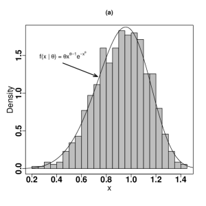
Figure 1.1: (a): Histogram (constructed based on chain’s output between 301$th$ up to 1000$th$ iterations); superimposed is ${\cal{W}}(\cdot|\theta=5,1)$ and (b): Chain’s motion across iterations for sampling from $f(x|\theta)={\cal{W}}(\theta=5,1)$ with starting value $x_{0}=4$.

1.2 Adaptive Metropolis-Hastings algorithm

The MCMC sampling techniques such as the MH algorithm are commonly widely used tools in a wide range of sciences. In some situations, the focus of primary concern is placed on the sampling from complicated high-dimensional distributions. In such cases tuning the parameters of the proposal distribution is of crucial importance. For example, suppose a zero-mean $p$-dimensional Gaussian distribution is chosen as the proposal so that ${\cal{S}}_{f}={\cal{S}}_{l}\in{\mathbb{R}}^{p}$. In practice, the true value of the proposal covariance is not known. The main challenge with Metropolis algorithm in this case is to find a good choice of the proposal covariance. Herein, the term good acceptance rate refers to the case that avoiding two challenging cases including 1: the chain visits all states rarely (generating highly correlated points) and 2: the chain visits all states frequently. Both of above two challenging cases result in generating highly correlated points. Hence, a suitable choice for covariance of proposal distribution is very important. The basic idea of introducing adaptive Metropolis (AM) algorithm is to update the proposal distribution using the information obtained so far about the target distribution. Let $\{\bm{x}_{0},\bm{x}_{1},\cdots,\bm{x}_{t-1}\}$ denote a sequence of $p$-dimensional samples generated until time $t-1$ in which $\bm{x}_{0}$ is the initial state (generation). The only difference between the AM and Metropolis algorithms is that in the former the sample $\bm{x}_{t}$ is drawn from symmetric PDF $l(\cdot|\bm{x}_{t-1})$ while in later the sample $\bm{x}_{t}$ is drawn from symmetric PDF $l(\cdot|\bm{x}_{0},\bm{x}_{1},\cdots,\bm{x}_{t-1})$. Clearly, in each AM algorithm, the pertaining stochastic chain is no longer Markovian and in fact $\bm{x}_{t}$ comes from, for example, a Gaussian distribution with mean $\bm{x}_{t-1}$ and covariance $C_{t}=C_{t}(\bm{x}_{0},\bm{x}_{1},\cdots,\bm{x}_{t-1})$. The main concern corresponds to adaptation is how to link the proposal covariance and $C_{t}$. This relation is represented as $C_{t}=s_{p}{\text{Cov}}(\bm{x}_{0},\bm{x}_{1},\cdots,\bm{x}_{t-1})+s_{p}\epsilon\bm{I}_{p}$ where where $s_{p}$ is a parameter that depends on $p$, $\epsilon$ is a small positive constant compared to size of ${\cal{S}}_{f}$, and $\bm{I}_{p}$ is a $p\times p$ identity matrix, see Haario et al. (2001). For practical purposes, one can chose an arbitrary strictly positive definite initial covariance $C_{0}$ based on user prior information and then consider index $t_{0}>0$ as the length of period. The covariance matrix of the proposal is then defined as

$$\displaystyle C_{t}=\left\{\begin{array}[]{c}\displaystyle C_{0},\leavevmode\nobreak\ \leavevmode\nobreak\ \leavevmode\nobreak\ \leavevmode\nobreak\ \leavevmode\nobreak\ \leavevmode\nobreak\ \leavevmode\nobreak\ \leavevmode\nobreak\ \leavevmode\nobreak\ \leavevmode\nobreak\ \leavevmode\nobreak\ \leavevmode\nobreak\ \leavevmode\nobreak\ \leavevmode\nobreak\ \leavevmode\nobreak\ \leavevmode\nobreak\ \leavevmode\nobreak\ \leavevmode\nobreak\ \leavevmode\nobreak\ \leavevmode\nobreak\ \leavevmode\nobreak\ \leavevmode\nobreak\ \leavevmode\nobreak\ \leavevmode\nobreak\ \leavevmode\nobreak\ \leavevmode\nobreak\ \leavevmode\nobreak\ \leavevmode\nobreak\ \leavevmode\nobreak\ \leavevmode\nobreak\ \leavevmode\nobreak\ \leavevmode\nobreak\ \leavevmode\nobreak\ \leavevmode\nobreak\ \leavevmode\nobreak\ \leavevmode\nobreak\ \leavevmode\nobreak\ \leavevmode\nobreak\ \leavevmode\nobreak\ \mathrm{{if}}\leavevmode\nobreak\ \leavevmode\nobreak\ \leavevmode\nobreak\ t\leq t_{0},\\ \displaystyle s_{d}{\text{Cov}}\bigl{(}\bm{x}_{0},\bm{x}_{1},\cdots,\bm{x}_{t-1}\bigr{)}+s_{d}\epsilon\bm{I}_{d},\leavevmode\nobreak\ \mathrm{if}\leavevmode\nobreak\ \leavevmode\nobreak\ \leavevmode\nobreak\ t>t_{0},\end{array}\right.$$

in which the empirical covariance matrix is

$${\text{Cov}}\bigl{(}\bm{x}_{0},\bm{x}_{1},\cdots,\bm{x}_{k}\bigr{)}=\frac{1}{k}\sum_{i=0}^{k}\bm{x}_{i}\bm{x}^{\top}_{i}-\frac{k+1}{k}\bar{\bm{x}}_{k}\bar{\bm{x}}^{\top}_{k}$$

for $\bar{\bm{x}}_{k}=1/(k+1)\sum_{i=0}^{k}\bm{x}_{i}$ with $\bm{x}_{i}\in\mathbb{R}^{p}$. The AM algorithm can be implemented quickly since for computing $C_{t}$ defined in above one can use the following recursion formula. For $t\geq t_{0}+1$, we have

$$C_{t+1}=\frac{t-1}{t}C_{t}+\frac{S_{p}}{t}\Bigl{(}t\bar{\bm{x}}_{t-1}\bar{\bm{x}}^{\top}_{t-1}-(t+1)\bar{\bm{x}}_{t}\bar{\bm{x}}^{\top}_{t}+\epsilon\bm{I}_{d}\Bigr{)}.$$

There are some more comments on AM algorithm (Haario et al., 2001) and its extensions such as adaptive proposal (Haario et al., 1999), adaptive Metropolis-within-Gibbs (Roberts and Rosenthal, 2009), regional adaptive Metropolis algorithm (Roberts and Rosenthal, 2009), and single component adaptive Metropolis algorithm (Haario et al., 2005). For useful accounts of AM algorithm and its extensions, the reader is referred to Atchadé and Rosenthal (2005); Andrieu and Atchadé (2006), (Roberts and Rosenthal, 2009), and references therein.

Chapter 2 Rejection sampling

2.1 Rejection sampling

Suppose sampling form PDF $f(\cdot|\theta)$ is not easy but it is dominated by another PDF such as $l(\cdot|\theta)$ so that

$$\underset{x\in{\cal{S}}_{f}}{\operatorname{sup}}\frac{f(x|\theta)}{l(x|\theta)}\leq c,$$

where $c\geq 1$ may depend on $\theta$. Finding a proposal PDF $l(x|\theta)$ that is as possible as close to $f(x|\theta)$ and easy-to-sample from would be the key objective in each rejection sampling scheme. The following four-step algorithm shows how a rejection sampling scheme works (Devroye, 1986a).

Algorithm 2 Rejection sampling technique

1:Choose suitable proposal with PDF $l(\cdot|\theta)$ and determine $c$;

2:Generate $y$ from $l(\cdot|\theta)$;

3:Generate $u$ from $\text{Unif}(0,1)$;

4:Squeezing test: If $u<\frac{f(y|\theta)}{c\times l(y|\theta)}$, then accept $y$ as a generation from $f(.|\theta)$, otherwise return to step 2 and repeat algorithm.

It is proved that average numbers of trials for generating a sample in each rejection sampling scheme is $1/c$, see Ross (2022). Figure 2.1(b) shows the chain’s motion across ${{K}}=1000$ iterations while the initial state is $x_{0}=4$. As it is seen, the convergence occurs very soon. There have been introduced some extensions of the MH algorithm in the literature. We refer reader to for more details about extensions such as (Robert et al., 2004; Roberts and Rosenthal, 2009; Robert et al., 2010).

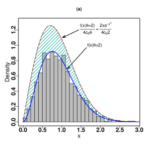
Figure 2.1: (a): Histogram constructed based on 1000 samples generated from ${\cal{W}}(\theta=2,1)$. Superimposed are $cl(x|\theta)$ (red line) and ${\cal{W}}(x|\theta=2,1)$ (blue line). (b): Generations across iterations for sampling from $f(x|\theta=2)={\cal{W}}(x|\theta=2,1)$.

Example 2 Suppose $f(x|\theta)$ is defined as in Example 1.1. Herein, we can rewrite $f(x|\theta)=(x+1)^{-2}x^{\theta}\exp\{-x^{\theta}\}/c_{0}$ where $c_{0}$ is normalizing constant guarantees $\int_{{\cal{S}}_{f}}f(x|\theta)dx=1$. Considering $l(x|\theta)={\cal{W}}(x|\theta,1)$ as the proposal, it is easy to check that

$$\frac{f(x|\theta)}{l(x|\theta)}=\frac{x}{c_{0}\theta(x+1)^{2}}.$$ (2.1)

Differentiating the RHS of (2.1) and setting the resultant to 0 reveals that the maximal value of RHS of (2.1) is $1/(4c_{0}\theta)$ that is obtained for $x=1$. That is

$$\frac{f(x|\theta)}{l(x|\theta)}\leq\frac{1}{4c_{0}\theta}=c.$$

It follows that

$$\frac{f(x|\theta)}{c\times l(x|\theta)}=\frac{4x}{(x+1)^{2}}.$$

Based on Algorithm 2, the rejection sampling scheme for generating realization from $f(\cdot|\theta=2)$ is described as follows.

1. Generate $y\sim{\cal{W}}(\theta=2,1)$;

2. Generate $u\sim\text{Unif}(0,1)$;

3. If $u<4y/(y+1)^{2}$, then accept $y$ as a generation from $f(\cdot|\theta=2)$; otherwise go to step 1 and repeat algorithm.

In Example 2.1 above, the usage time study for generating $N=1000$ realization is around 0.01 second. The pertaining R code, for producing Figure 2.1(b), is given as follows.

⬇

1R > set.seed(20240519)

2R > N <- 10000 # size of generations

3R > theta <- 2

4R > w <- rep(0, N) # vector of generated realizations

5R > j <- 1

6R > while(j <= N)

7+ {

8+ y <- rweibull(1, shape = theta, scale = 1)

9+ u <- runif(1)

10+ if( u < 4*y/(y+1)^2 )

11+ {

12+ w[j] <- y # y is accepted

13+ j <- j + 1

14+ }

15+ }

16R > plot(w)

Example 3 Let random variable $X$ follow a distribution with PDF given by Azzalini (1985):

$$f(x|\mu,\sigma,\lambda)=\frac{2}{\sigma}\phi\Bigl{(}\frac{x-\mu}{\sigma}\Bigr{)}\Phi\Bigl{(}\lambda\frac{x-\mu}{\sigma}\Bigr{)},$$ (2.2)

where $\phi(\cdot)$ and $\Phi(\cdot)$ represent accordingly the PDF and CDF of the standard Gaussian distribution. Herein, $\lambda\in{\mathbb{R}}$ is the skewness parameter (the cases $\lambda\rightarrow-\infty$, $\lambda=0$, and $\lambda\rightarrow+\infty$ yield totally skewed to the left, symmetric (ordinary Gaussian), and totally skewed to the right distributions, respectively), $\mu\in{\mathbb{R}}$ is the location parameter, and $\sigma\in{\mathbb{R}}^{+}$ denotes the scale parameter. Hereafter, we write ${\cal{SG}}(\mu,\sigma,\lambda)$ to denote the distribution with PDF given by (2.2). Without loss of generality, let $\mu=0$ and $\sigma=0$. A direct method proposed by Henze (1986) for simulating from ${\cal{SG}}(0,1,\lambda)$ as follows. Let $Z_{1}$ and $Z_{1}$ denote two independent copy of standard Gaussian random variate. Then random variable $X$ given by

$$X=\frac{\lambda\big{|}Z_{1}\big{|}+Z_{2}}{\sqrt{1+\lambda^{2}}}.$$ (2.3)

follows ${\cal{SG}}(0,1,\lambda)$ distribution. For simulating from ${\cal{SG}}(0,1,\lambda)$ using the rejection method, we proceed by considering the fact that

$$f(x|0,1,\lambda)\leq 2l(x|\lambda)=2\phi(x).$$ (2.4)

Hence, simulating from ${\cal{SG}}(\mu,\sigma,\lambda)$, through the rejection sampling, is possible by considering the proposal PDF to be $\phi(x)$ and $M=2$. Figure 2.2(a) shows histogram of generated realizations as well as the superimposed target and proposal PDFs for $\lambda=4$. The sampler’s motion across 500 iterations are displayed in Figure 2.1(b).

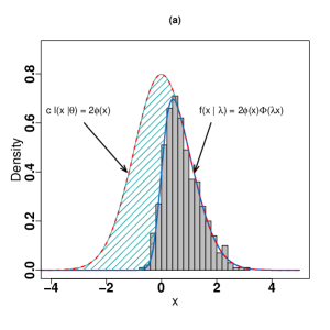
Figure 2.2: (a): Histogram constructed based on 500 samples generated from ${\cal{SG}}(0,1,\lambda=4)$. Superimposed are $cl(x|\theta)=2\phi(x)$ (red line) and ${\cal{SG}}(x|0,1,\lambda=4)$ (blue line). (b): Generations across iterations for sampling from $f(x|\theta=4)={\cal{SG}}(0,1,\lambda=4)$.

The pertaining R code, for producing Figure 2.2(b), is given as follows.

⬇

1R> set.seed(20240225)

2R> N <- 500

3R> i <- 1; x <- rep(0, N); lambda <- 4

4R> while(i <= N)

5+ {

6+ z <- rnorm(1);

7+ if( runif(1) < pnorm(lambda*z) )

8+ {

9+ x[i] <- z; i <- i + 1

10+ }

11+ }

12R > plot(x)

2.2 Adaptive rejection sampling

Suppose $f(x|\theta)$ is a log-concave PDF over ${\cal{S}}_{f}$ that equivalently means ${\cal{H}}(x)=\log f(x|\theta)$ is a concave function of $x$. A method was proposed by Devroye (1986b) for generating realization form log-concave distribution provided that the mode (a point at which derivative of $f(x|\theta)$ with respect to $x$ is zero) of $f(x|\theta)$ to be known. More precisely, the proposed method is a rejection sampling scheme using a three-piece exponential proposal in which the center piece touches the target PDF $f(x|\theta)$ at its mode. While this method is not adaptive, the adaptive rejection sampling (ARS) scheme (Gilks and Wild, 1992) develops this method by improving the proposal distribution in each iteration such that the updated proposal proposes generation that passes the squeezing test with higher probability than the previous iteration. In each ARS scheme, ${\cal{H}}(x)$ can be bounded by piecewise linear upper hull in which each tangent line is defined as

$$U_{k}(x)=(x-a){\cal{H}}^{\prime}(a)+{\cal{H}}(a),$$ (2.5)

for $x\in[z_{i-1},z_{i}]$ and $i=1,\cdots,k$ where

$$z_{i}=\frac{{\cal{H}}\bigl{(}x_{i+1}\bigr{)}-{\cal{H}}\bigl{(}x_{i}\bigr{)}-x_{i+1}{\cal{H}}^{\prime}\bigl{(}x_{i+1}\bigr{)}+x_{i}{\cal{H}}^{\prime}\bigl{(}x_{i}\bigr{)}}{{\cal{H}}^{\prime}\bigl{(}x_{i}\bigr{)}-{\cal{H}}^{\prime}\bigl{(}x_{i+1}\bigr{)}}.$$

We note that the tangent lines are constructed at abscissa (points) $T_{k}=\{x_{1}\leq x_{2}\leq\cdots\leq x_{k}\in{\cal{S}}_{f}\}$ and intersect at $z_{i}$ where $z_{0}$ and $z_{k}$ are the lower ($-\infty$ if ${\cal{S}}_{f}$ is not bounded from below) and the upper ($\infty$ if ${\cal{S}}_{f}$ is not bounded from above) bounds of ${\cal{S}}_{f}$, accordingly. Likewise, we can define a piecewise linear lower hull constructed based on chords between adjacent abscissae in $T_{k}$ as

$$L_{k}(x)=\frac{{\cal{H}}\bigl{(}x_{i+1}-x\bigr{)}{\cal{H}}\bigl{(}x_{i}\bigr{)}-{\cal{H}}\bigl{(}x-x_{i}\bigr{)}{\cal{H}}\bigl{(}x_{i+1}\bigr{)}}{x_{i+1}x_{i}},$$ (2.6)

where $x\in[x_{i},x_{i+1}]$ for $i=1,\cdots,k-1$. If $x<x_{1}$(or $x>x_{k}$), then we set $L_{k}(x)=-\infty$. Notice that log-concavity of $f(x|\theta)$ ensures that $L_{k}(x)\leq{\cal{H}}(x)\leq U_{k}(x)$ for $x\in{\cal{S}}_{f}$. Each ARS algorithm proceeds three initialization, sampling, and updating steps for generating $n$ realizations from PDF $f(x|\theta)$ given by the following.

• initialization step: Construct the abscissae in $T_{k}$. If ${\cal{S}}_{f}$ is left-unbounded, then set $x_{1}$ such that ${\cal{H}}^{\prime}\bigl{(}x_{1}\bigr{)}<0$ and if ${\cal{S}}_{f}$ is right-unbounded, then set $x_{k}$ such that ${\cal{H}}^{\prime}\bigl{(}x_{k}\bigr{)}<0$. Furthermore, compute $L_{k}(x)$, $U_{k}(x)$, and $S_{k}(x)$ where

  $$s_{k}(x)=\frac{\exp\{U_{k}(x)\}}{\int\exp\{U_{k}(y)\}dy},$$

  and functions $L_{k}(x)$ and $U_{k}(x)$ as defined in (2.6) and (2.5), accordingly.

• sampling step: Generate $x^{*}$ from $s_{k}(x)$ and $u\sim\text{Unif}(0,1)$ independently; and then perform squeezing test that accepts $x^{*}$ if $w\leq\exp\{L_{k}(x^{*})-U_{k}(x^{*})\}$; otherwise compute the rejection test that accepts $x^{*}$ if $w\leq\exp\{{\cal{H}}\bigl{(}x^{*}\bigr{)}-U_{k}(x^{*})\}$; otherwise reject $x^{*}$.

• updating step: If evaluating ${\cal{H}}\bigl{(}x^{*}\bigr{)}$ and ${\cal{H}}^{\prime}\bigl{(}x^{*}\bigr{)}$ is necessary, then add $x^{*}$ to $T_{k}$ in order to form updated $T_{k}$ as $T^{*}_{k}=\bigl{\{}\{x_{1}\leq x_{2}\leq\cdots\leq x_{k}\}\cup x^{*}\in{\cal{S}}_{f}\bigr{\}}$. Return to the initialization step while the set of $k+1$ abscissae in $T^{*}_{k}$ is relabeled in ascending order and repeat these three steps if $n$ realizations have been not yet obtained. We note that for initialization, a set of two starting abscissae $(k\geq 2)$ is necessary.

We note that a given PDF $f(.|\theta)$ is unimodal if and only if $f(.|\theta)$ is log-concave. So, for simulating from a distribution with unimodal PDF $f(.|\theta)$, the ARS algorithm would be a suitable candidate provided that ${\cal{H}}(.)$ has closed form.

Example 4 Let $f(x|\bm{\theta})$ represent the PDF of generalized inverse Gaussian (denoted as $GIG(a,b,c)$) distribution defined as

$$f(x|\bm{\theta})=\Bigl{(}\frac{b}{c}\Bigr{)}^{\frac{a}{2}}\frac{x^{c-1}}{2{\cal{K}}_{a}(\sqrt{bc})}\exp\Bigl{\{}-\frac{bx}{2}-\frac{c}{2x}\Bigr{\}},$$ (2.7)

where $\bm{\theta}=(a,b,c)^{\top}$. It is easy to check that $f(x|\bm{\theta})$ is log-concave for $a\geq 1$. Implementing the ARS algorithm is executable through the computer code. For R environment, the package ars developed for this purpose that is available at https://CRAN.R-project.org/package=ars.

2.3 Two-dimensional single rejection sampling

Let $f(x|{\theta})$, that my be known only up to a proportionality constant $z$, is an unimodal PDF of random variable $X\in\mathbb{R}$ from which sampling is of interest. If it is possible to consider an extra auxiliary variable $Y$, thereby the marginal PDF o $X$ can be marginalized by integrating out $Y$ as

$$f(x|{\theta})=\int f(x,y|{\theta})dy,$$

then one can use the two-dimensional rejection sampling scheme in order to generate sample $x$ with PDF $f(x|{\theta})$. For this purpose, let $l(x,y|\theta)$ denote the joint PDF of the proposal (candidate) such that

$$\underset{(x,y)\in{\cal{S}}_{f(x,y|\theta)}}{\operatorname{sup}}\frac{f(x,y|\theta)}{l(x,y|\theta)}=c.$$

We use the following algorithm for simulating from $f(x|{\theta})$ through the two-dimensional single rejection sampling scheme.

1. Generate pair $(X,Y)$ or the joint PDF $l(x,y\theta)$;

2. Generate $u\sim\text{Unif}(0,1)$;

3. If $u<f(x,y|\theta)/\bigl{[}c\times l(x,y|\theta)\bigr{]}$, then accept $X$ as a generation from $f(x|\theta)$; otherwise return to step 1 and repeat the algorithm.

The efficiency of a two-dimensional single rejection sampling scheme depends on quantity $c$ and the complexity of sampling from two-dimensional candidate $l(x,y|\theta)$. If $l(x,y|\theta)$ is easy to sampling from and $c$ is as small as possible, then this algorithm works efficiently.

Example 5 Let $X$ denotes a random variable following an exponentially tilted $\alpha$-stable distribution with tilting parameter $\lambda>0$ if it follows a distribution whose PDF is given by

$$f(x|\bm{\theta})=\exp\bigl{\{}-x\lambda+\lambda^{\frac{\alpha}{2}}\bigr{\}}d(x|\alpha),$$ (2.8)

where $\bm{\theta}=(\alpha,\lambda)^{\top}$ for $0<\alpha\leq 2$ is the family parameter vector and $d(x|\alpha)$ is the PDF of a positive $\alpha$-stable distribution, see Devroye (2009). The PDF $d(x|\alpha)$ has not closed form, but can be represented as

$$d(x|\alpha)=\frac{1}{\pi}\int_{0}^{\pi}\exp\Bigl{\{}-x^{-\frac{\alpha}{2-\alpha}}[A(y)]^{1-\frac{\alpha}{2}}\Bigr{\}}dy,$$ (2.9)

where $A(y)$ in RHS of (2.9) is called the Zolotarev’s function (Devroye, 2009) defined as

$$A(y)=\left[\frac{\Bigl{\{}\sin\bigl{[}\bigl{(}\frac{\alpha}{2}\bigr{)}y\bigr{]}\Bigr{\}}^{\frac{\alpha}{2}}\Bigl{\{}\sin\Bigl{[}\bigl{(}1-\frac{\alpha}{2}\bigr{)}y\Bigr{]}\Bigr{\}}^{1-\frac{\alpha}{2}}}{\sin(y)}\right]^{\frac{2}{2-\alpha}}.$$

From (2.8) and (2.9), it can be easily seen that $f(x|\bm{\theta})$ is the marginal of a joint PDF. Herein, we do not aim to discuss this example in details and just mention that for simulating from $f(x,y|\bm{\theta})$, a bivariate distribution with PDF

$$l(x,y|\bm{\theta})=\frac{1}{\pi}\times\frac{x^{m-1}}{\Gamma(m)}\exp\{-x\},$$ (2.10)

is chosen as candidate. Depending on values of $\alpha$ and $\lambda$, the gamma PDF with shape parameter $m=\alpha\lambda^{\alpha}$ in RHS of (2.10) can be replaced with a gamma PDF with shape parameter $m=(1-\alpha)\lambda^{\alpha}+1$ or truncated Gaussian PDF. The reader is referred to (Hofert, 2011; Qu et al., 2021) for a thorough treatment of this example. For simulating from PDF (2.8), there is an open source code called copula has been developed for R language that is available at https://CRAN.R-project.org/package=copula.

Chapter 3 Importance Sampling

The Monte Carlo techniques essentially can be seen as a tool for computing single or multiple integrals. This feature of the Monte Carlo techniques that focuses on computing integrals is called importance sampling. It is worth noting that, contrary to its name, the importance sampling does not proceed to sample from a statistical distribution, but also aims to compute an integral. This concern of this chapter is placed on computing the single and multiple integrals that are widely used in statistical analyses.

3.1 Importance sampling

Let $h(x)$ to be a continuous real function and $f(x)$ is a given PDF. Suppose we would like to compute the expectation

$$E_{f}\bigl{(}h(X)\bigr{)}=\int_{\mathbb{R}}h(x)f(x)dx,$$ (3.1)

where the generic symbol $E_{f}(h(X))$ indicates that the expectation of random variable $h(X)$ is computed when $X$ follows the PDF $f$. Usually, computing (3.1) directly is not a simple task and mus be evaluated numerically. The importance sampling is a tool to get round this difficulty. To this end, notice that the integral (3.1) can be rewritten as

$$E_{f}\bigl{(}h(X)\bigr{)}=\int_{\mathbb{R}}h(y)\frac{f(y)}{g(y)}g(y)dy=E_{g}\Bigl{(}h(X)\frac{g(X)}{f(X)}\Bigr{)}=E_{g}\bigl{(}h(X)w(X)\bigr{)},$$ (3.2)

where $w(u)=f(u)/g(u)$. Herein, the PDF $g(\cdot)$ is called the importance or instrumental PDF and its support dominates that of the PDF $f(x)$, that is ${\cal{S}}_{f}\subset{\cal{S}}_{g}$. By the law of large numbers, the RHS of (3.2) is estimated as

$$\hat{\mu}=\widehat{E_{f}\bigl{(}h(X)\bigr{)}}=\frac{1}{n}\sum_{i=1}^{n}w(x_{i})h(x_{i}),$$ (3.3)

where $x_{1},\cdots,x_{n}$ come independently from PDF $g(\cdot)$. Hence, by generating a large number of realizations from PDF $g(\cdot)$ the preceding expectation is approximated well. for a wide ranges of applications the target PDF $f(\cdot)$ is just known up to a normalization constant. In such cases, estimator of $E_{f}\bigl{(}h(X)\bigr{)}$ is given by

$$\tilde{\mu}=\widetilde{E_{f}\bigl{(}h(X)\bigr{)}}=\frac{\sum_{i=1}^{n}w(x_{i})h(x_{i})}{\sum_{i=1}^{n}w(x_{i})},$$ (3.4)

that is self-normalized. The bias and variance of both estimators $\hat{\mu}$ and $\tilde{\mu}$ can be evaluated (Liu and Liu, 2001). We have

$$E_{g}\bigl{(}\hat{\mu}\bigr{)} =\mu$$ (3.5)

$$E_{g}\bigl{(}\tilde{\mu}\bigr{)} \approx\mu+\frac{\mu\times\text{var}_{g}(w(X))-\text{cov}_{g}\bigl{(}w(X),w(X)h(X)\bigr{)}}{n}$$ (3.6)

and

$$\text{var}_{g}\bigl{(}\hat{\mu}\bigr{)} =\frac{\text{var}_{g}\bigl{(}w(X)h(X)\bigr{)}}{n}$$ (3.7)

$$\text{var}_{g}\bigl{(}\tilde{\mu}\bigr{)} \approx\frac{\text{var}_{g}\bigl{(}w(X)h(X)\bigr{)}-2\mu\times\text{cov}_{g}\bigl{(}w(X),w(X)h(X)\bigr{)}+\mu^{2}\times\text{var}_{g}\bigl{(}w(X)\bigr{)}}{n}$$ (3.8)

It is clear from (3.5) and (3.6) that $\hat{\mu}$ is unbiased estimator for $\mu$ while the estimator $\tilde{\mu}$ is biased. Of course, in some situations the variance (standard error) of the self-normalized estimator $\tilde{\mu}$, as it is seen from RHS of (3.7), can be smaller than that of $\hat{\mu}$ that is given by (3.8). The main feature in each importance sampling problem is to determine the instrumental PDF $g(\cdot)$. Although, theoretically, there are many choices of $g(\cdot)$, but we have to find the best choice that yields as small as possible standard error for $\hat{\mu}$ (or $\tilde{\mu}$). Fortunately, there is a specific rule available for this purpose. It is proved that the optimal choice $g_{o}(x)$ becomes (Johansen et al., 2010):

$$g_{o}(x)=\frac{|h(x)|f(x)}{\int_{\mathbb{R}}|h(u)|f(u)du}.$$ (3.9)

Example 6 Suppose we are interested in computing ${{\Omega}}=E\bigl{(}\log(1+X)\bigr{)}$ where $X\sim{\cal{G}}(\alpha,\beta)$. We may choose three instrumentals as: 1- exponential distribution with rate parameter $\beta$, say ${\cal{E}}(\beta)$, 2- gamma distribution, say ${\cal{G}}(\alpha,\beta)$, and the optimal one with PDF $g_{0}(x)=h(x){\cal{G}}(x|\alpha,\beta)$. Under the first choice, we have

$$\hat{\Omega}=\frac{\beta^{\alpha-1}}{\Gamma(\alpha)}\frac{1}{N}\sum_{i=1}^{N}x_{i}^{\alpha-1}\log(x_{i}+1)$$ (3.10)

where $x_{i}$s come independently from ${\cal{E}}(\beta)$. In the case of second choice of instrumental, we have

$$\hat{\Omega}=\frac{1}{N}\sum_{i=1}^{N}x_{i},$$ (3.11)

where $x_{i}$s come independently ${\cal{G}}(\alpha,\beta)$. In the case of $g_{o}(x)$ and ${\cal{SG}}(0,1,\lambda)$, respectively. and second choices of instrumental, we have

$$\hat{\Omega}=N\biggl{[}\sum_{i=1}^{N}\frac{1}{\log\bigl{(}x_{i}+1\bigr{)}}\biggr{]}^{-1},$$ (3.12)

where $x_{i}$s come independently from PDF given by (3.13).

$$g_{o}(x)=\frac{\log(x+1){\cal{G}}(x|\alpha,\beta)}{\int_{0}^{\infty}\log(u+1){\cal{G}}(u|\alpha,\beta)du},$$ (3.13)

For sampling from $g_{o}(x)$ given above, we designate a rejection scheme given by the following steps.

1. Sample realization $y$ from ${\cal{G}}(\alpha+1,\beta)$ as the proposal distribution;

2. Sample independent realization $u$ from ${\cal{U}}(0,1)$;

3. if $y<\log(y+1)/y$, then accept $y$ as a generation from PDF $g_{o}(x)$ given by (3.13); otherwise return to step (1) an repeat this procedure until having acceptance.

The R function rlgamma, given below, generates sample from $g_{o}(x)$ based on above rejection scheme.

⬇

1R> rlgamma <- function(N, alpha, beta)

2+ {

3+ g <- rep(0, N) # vector of generated realizations

4+ j <- 1

5+ while(j <= N)

6+ {

7+ y <- rgamma(1, shape = alpha + 1, rate = beta)

8+ u <- runif(1)

9+ A <- log(y+1)/(y)

10+ if( u < A )

11+ {

12+ g[j] <- y # y is accepted

13+ j <- j + 1

14+ }

15+ }

16+ return(g)

17+ }

Table 3.1 represents the results of simulation study based on $M=5000$ runs of samples each of size $N=5000$. It follows from this table that the second instrumental, that is ${\cal{SG}}(0,1,\lambda)$, gives the best summary. Not surprisingly, the optimal instrumental does not work as well as or better than others since ${\text{var}}_{g_{o}}\bigl{(}W(X)\bigr{)}$ is inflated by the small values in the generated data from this instrumental. It is worth noting that the $g_{o}(\cdot)$ works well if $W(x)=f(x)/g_{o}(x)$ is bounded. For our case, this condition may fail since $W(x)=f(x)/g_{o}(x)=1/|x|$ becomes large in presence of even a few number of small realizations. Table 3.1: The summary statistics for computing $\Omega=E\bigl{(}\log(1+X)\bigr{)}$ where $X\sim{\cal{G}}(\alpha,\beta)$ through three instrumentals. summary $(\alpha,\beta)$ $\Omega$ instrumental bias SE minimum maximum (0.5,0.5) 0.6695 ${\cal{E}}(\beta)$ 1.1e-04 5.4e-05 0.5047 0.5611 ${\cal{G}}(\alpha,\beta)$ -4.9e-05 3.4e-06 0.5271 0.5404 $g_{o}$ 6.2e-03 1.9e-03 0.0649 0.6249 (0.5,5) 0.0884 ${\cal{E}}(\beta)$ -4.8e-05 -4.9-05 0.0830 0.0948 ${\cal{G}}(\alpha,\beta)$ -5.9e-07 -5.9e-07 0.0864 0.0902 $g_{o}$ 1.4e-03 1.5e-03 0.0066 0.1076 (5,0.5) 2.3152 ${\cal{E}}(\beta)$ 1.2e-04 3.4e-05 2.2940 2.3356 ${\cal{G}}(\alpha,\beta)$ -4.1e-03 1.2e-01 1.4422 6.0980 $g_{o}$ -2.9e-05 -4.1e-05 2.2926 2.3363 (5,5) 0.6695 ${\cal{E}}(\beta)$ -1.8e-05 3.4e-05 0.6586 0.6814 ${\cal{G}}(\alpha,\beta)$ 1.1e-03 1.1e-01 0.4109 1.5190 $g_{o}$ 1.2e-05 4.1e-05 0.6562 0.6848

Next example shows that if above conditions are not met, then the importance sampling using the optimal choice $g_{o}(\cdot)$ may fail to show the best performance.

Example 7 Suppose we would like to compute $\Omega=E(|X|)$ where $X\sim{\cal{SG}}(0,1,\lambda)$ and expression of ${\cal{SG}}(x|0,1,\lambda)$ is given by (2.2). To this end, we consider three instrumentals including: ${\cal{N}}(0,1)$, ${\cal{SG}}(0,1,\lambda)$, and $g_{o}(x)$. The PDF of the latter is given by

$$g_{o}(x)=\frac{2|x|\phi(x)\Phi(\lambda x)}{\int_{-\infty}^{\infty}2|u|\phi(u)\Phi(\lambda u)du},$$ (3.14)

where quantity $c$ plays the role of normalizing constant. But, first, we need to simulate from $g_{o}(x)$ given by (3.14). In what follows we give two methods for this purpose without proof.

1. Sample independent realizations $z_{1}$ and $z_{2}$ from ${\cal{N}}(0,1)$;

2. Sample independent realization $u\sim{\cal{U}}(0,1)$;

3. if $z_{1}<\lambda z_{2}$ and $4u<\big{|}z_{2}\big{|}$, then accept $z_{2}$ as a generation from PDF (3.14); otherwise return to step (1) an repeat this procedure until having acceptance.

The second method is as follows.

1. Sample realization $w\sim{\cal{W}}(2,1/\sqrt{2})$;

2. Sample independent realization $u\sim{\cal{U}}(0,1)$;

3. If $u<\Phi(\lambda w)$, then accept $w$ as a generation from PDF (3.14); otherwise accept $-w$ as a generation from PDF (3.14).

Evidently, the second algorithm is more efficient than the first one in terms of the time of implementing. For computing $\hat{\Omega}$, we consider under the first choice of instrumental, we have

$$\hat{\Omega}=\frac{2}{N}\sum_{i=1}^{N}\big{|}x_{i}\big{|}\Phi\bigl{(}\lambda x_{i}\bigr{)},$$ (3.15)

where $x_{i}$s come independently from ${\cal{N}}(0,1)$. In the case of second choice of instrumental, we have

$$\hat{\Omega}=\frac{1}{N}\sum_{i=1}^{N}x_{i},$$ (3.16)

where $x_{i}$s come independently ${\cal{SG}}(0,1,\lambda)$, respectively. In the case of $g_{o}(x)$ and ${\cal{SG}}(0,1,\lambda)$, respectively. and second choices of instrumental, we have

$$\hat{\Omega}=N\Bigl{[}\sum_{i=1}^{N}\frac{1}{\big{|}x_{i}\big{|}}\Bigr{]}^{-1},$$ (3.17)

where $x_{i}$s come independently from PDF given by (3.14). Table represents the results of simulation study based on 5000 runs of samples each of size $N=5000$. As it may be seen from Table 3.2, overall, the second instrumental, that is ${\cal{SG}}(0,1,\lambda)$, gives the best summary. Not surprisingly, the optimal instrumental does not work as well as or better than others since ${\text{var}}_{g_{o}}\bigl{(}W(X)\bigr{)}$ is inflated by the small values in the generated data from this instrumental. It is worth noting that the $g_{o}(\cdot)$ works well if $W(x)=f(x)/g_{o}(x)$ is bounded. For our case, this condition may fail since $W(x)=f(x)/g_{o}(x)=1/|x|$ becomes large in presence of even a few number of small realizations. Table 3.2: The summary statistics for computing $\Omega=E(|X|)$ where $X\sim{\cal{SG}}(0,1,\lambda)$ through three instrumentals. summary $\lambda$ instrumental bias SE minimum maximum $\lambda=0$ ${\cal{N}}(0,1)$ 5.1e-05 0.0083 0.7688 0.8250 ${\cal{SG}}(0,1,\lambda=0)$ 3.8e-05 0.0084 0.7663 0.8259 $g_{o}(\cdot)$ 1.0e-03 0.0218 0.4925 0.8574 $\lambda=5$ ${\cal{N}}(0,1)$ 4.3e-04 0.0168 0.7267 0.8560 ${\cal{SG}}(0,1,\lambda=5)$ 3.5e-05 0.0084 0.7693 0.8290 $g_{o}(\cdot)$ 1.1e-03 0.0214 0.5341 0.8573 $\lambda=10$ ${\cal{N}}(0,1)$ 7.2e-05 0.0165 0.7367 0.8553 ${\cal{SG}}(0,1,\lambda=10)$ 2.9e-05 0.0084 0.7683 0.8311 $g_{o}(\cdot)$ 6.9e-04 0.0221 0.2998 0.8533

3.2 Computing the CDF of Gaussian distribution

In this section, we proceed to provide the compute the Monte Carlo approximation for the CDF of the Gaussian distribution.

3.2.1 Computing the CDF of univariate Gaussian distribution

Indeed computing the CDF of a Gaussian distribution is an importance sampling problem. Following example gives more detailed information.

Example 8 Let $Z\sim{\cal{N}}(0,1)$ and we are interested in computing $P(Z<2)$. Evidently the given probability can be represented as

$$P(Z<2) =\frac{1}{\sqrt{2\pi}}\int_{-\infty}^{2}\exp\Bigl{\{}-\frac{z^{2}}{2}\Bigr{\}}dz$$

$$=\frac{1}{\sqrt{2\pi}}\int_{-\infty}^{\infty}\mathbb{I}_{(-\infty,2)}(z)\times\exp\Bigl{\{}-\frac{z^{2}}{2}\Bigr{\}}dz$$

$$=E\Bigl{(}\mathbb{I}_{(-\infty,2)}(Z)\Bigr{)},$$ (3.18)

where $\mathbb{I}_{{\cal{S}}}(x)$ is the well-known indicator function defined as

$$\displaystyle\mathbb{I}_{{\cal{S}}}(x)=\left\{\begin{array}[]{c}\displaystyle 1,\leavevmode\nobreak\ \leavevmode\nobreak\ \mathrm{{if}}\ x\in{\cal{S}},\\ \displaystyle 0,\leavevmode\nobreak\ \leavevmode\nobreak\ \mathrm{if}\ x\notin{\cal{S}}.\end{array}\right.$$ (3.21)

Hence, the quantity can be readily approximated by considering the standard univariate Gaussian as the instrumental distribution. It follows that

$$P(Z<2) \approx\frac{1}{N}\sum_{i=1}^{N}\mathbb{I}_{(-\infty,2)}\bigl{(}z_{i}\bigr{)}=\frac{{\text{number of $z_{i}$s less that 2 with a sample of size $N$}}}{N},$$ (3.22)

where $z_{1},\cdots,z_{N}$ independently follow ${\cal{N}}(0,1)$ and $N$ is a sufficiently large integer value. This means that the Monte Carlo approximation of $P(Z<2)$ given in (3.22) is the average of samples that are less than two. The Central limit theorem guarantees that estimator (3.22) is unbiased for $P(Z<2)$ with variance

$$\frac{\Phi(2|0,1)\bigl{[}1-\Phi(2|0,1)\bigr{]}}{N}.$$

Of course, the command integrate(f, lower, upper, ...) (when f is the PDF of Gaussian distribution) or pnorm(q, mean = 0, sd = 1,...) can be used in R environment for computing the CDF of Gaussian distribution. However, one could use the well known Gaussian quadrature rules discussed in next Chapter.

3.3 Computing the CDF of multivariate Gaussian distribution

Due to significant importance of the multivariate Gaussian distribution in a wide range of study fields, computing its CDF has a long history. Several efforts have been made for computing the CDF of multivariate Gaussian distribution. For more detailed information, we refer the reader to Botev (2017) and references therein. One of the pioneers in this context was Genz (1992) who suggested the separation of variables (SOV) method. Let $\bm{X}\sim{\cal{N}}_{p}(\bm{\mu},\Sigma)$ and $L$ denote the Cholesky decomposition of $\Sigma$, that is $\Sigma=LL^{\top}$ in which $L$ is a $p\times p$ lower triangular matrix. For computing ${\cal{P}}=P(\bm{a}<\bm{X}<\bm{b})$, in which $\bm{a}$ and $\bm{b}$ are vectors of real constants, the SOV method can be described as follows. Consider transformation $\bm{x}=L\bm{y}$, we have

$$\bm{x}^{\top}\Sigma^{-1}\bm{x}=\bm{y}^{\top}L^{\top}L^{-\top}L^{-1}L\bm{y}=\bm{y}^{\top}\bm{y}=\sum_{i=1}^{p}y^{2}_{i},$$

and $d\bm{x}=|L|\bm{y}=\Sigma^{1/2}\bm{y}$. Hence, $\bm{a}<L\bm{y}<\bm{b}$ or equivalently

$$\frac{a_{1}}{L_{1,1}}\leq {y}_{1} \leq\frac{b_{1}}{L_{1,1}}$$

$$\frac{a_{2}-L_{2,1}y_{1}}{L_{2,2}}\leq {y}_{2} \leq\frac{b_{2}-L_{2,1}y_{1}}{L_{2,2}}$$

$$\vdots$$

$$\frac{a_{p}-\sum_{i=1}^{p-1}L_{p,i}y_{i}}{L_{p,p}}\leq {y}_{p} \leq\frac{b_{p}-\sum_{i=1}^{p-1}L_{p,i}y_{i}}{L_{p,p}}.$$

This type of change of variable reduces the problem of computing ${\cal{P}}$ to $p$ univariate integration as follows.

$${\cal{P}}=(2\pi)^{-\frac{p}{2}}\int_{a_{1}^{\prime}}^{b_{1}^{\prime}}\exp\Bigl{\{}-\frac{y_{1}^{2}}{2}\Bigr{\}}\int_{a_{2}^{\prime}}^{b_{2}^{\prime}}\exp\Bigl{\{}-\frac{y_{2}^{2}}{2}\Bigr{\}}\cdots\int_{a_{p}^{\prime}}^{b_{p}^{\prime}}\exp\Bigl{\{}-\frac{y_{m}^{2}}{2}\Bigr{\}}d\bm{y},$$ (3.23)

where $a^{\prime}_{i}=\bigl{(}a_{i}-\sum_{j=1}^{i-1}L_{i,j}y_{j}\bigr{)}/L_{i,i}$ and $b^{\prime}_{i}=\bigl{(}b_{i}-\sum_{j=1}^{i-1}L_{i,j}y_{j}\bigr{)}/L_{i,i}$. By applying another transformation of the form $z_{i}=\Phi\bigl{(}y_{i}\bigr{)}$ (for $i=1,\cdots,p$), we obtain

$${\cal{P}}=\int_{d_{1}}^{e_{1}}\int_{d_{2}}^{e_{2}}\cdots\int_{d_{p}}^{e_{p}}d\bm{z},$$ (3.24)

where

$$d_{i}= \Phi\biggl{(}\frac{a_{i}-\sum_{j=1}^{i-1}L_{i,j}\Phi^{-1}(z_{j})}{L_{i,i}}\biggr{)},$$

$$e_{i}= \Phi\biggl{(}\frac{b_{i}-\sum_{j=1}^{i-1}L_{i,j}\Phi^{-1}(z_{j})}{L_{i,i}}\biggr{)}.$$

Although the integrand in (3.24) has a simpler form than (3.23), but its integral region is complicated. As a solution for this issue, we apply the transformation $w_{i}=(z_{i}-d_{i})/(e_{i}-d_{i})$ to see that

$${\cal{P}} =\int_{0}^{1}\bigl{(}e^{\prime}_{1}-d^{\prime}_{1}\bigr{)}d{w_{1}}\int_{0}^{1}\bigl{(}e^{\prime}_{2}-d^{\prime}_{2}\bigr{)}d{w_{2}}\cdots\int_{0}^{1}\bigl{(}e^{\prime}_{p-1}-d^{\prime}_{p-1}\bigr{)}d{w_{p-1}}\int_{0}^{1}\bigl{(}e^{\prime}_{p}-d^{\prime}_{p}\bigr{)}d{w_{p}},$$

$$=\bigl{(}e^{\prime}_{1}-d^{\prime}_{1}\bigr{)}\int_{0}^{1}\bigl{(}e^{\prime}_{2}-d^{\prime}_{2}\bigr{)}d{w_{1}}\int_{0}^{1}\bigl{(}e^{\prime}_{3}-d^{\prime}_{3}\bigr{)}d{w_{2}}\cdots\int_{0}^{1}\bigl{(}e^{\prime}_{p}-d^{\prime}_{p}\bigr{)}d{w_{p-1}}\int_{0}^{1}d{w_{p}},$$

$$=\bigl{(}e^{\prime}_{1}-d^{\prime}_{1}\bigr{)}\int_{0}^{1}\bigl{(}e^{\prime}_{2}-d^{\prime}_{2}\bigr{)}d{w_{1}}\int_{0}^{1}\bigl{(}e^{\prime}_{3}-d^{\prime}_{3}\bigr{)}d{w_{2}}\cdots\int_{0}^{1}\bigl{(}e^{\prime}_{p}-d^{\prime}_{p}\bigr{)}d{w_{p-1}},$$ (3.25)

where

$$d^{\prime}_{i}= \Phi\biggl{(}\frac{a_{i}-\sum_{j=1}^{i-1}L_{i,j}\Phi^{-1}\bigl{(}d_{j}+w_{j}(e_{j}-d_{j})\bigr{)}}{L_{i,i}}\biggr{)},$$

$$e^{\prime}_{i}= \Phi\biggl{(}\frac{b_{i}-\sum_{j=1}^{i-1}L_{i,j}\Phi^{-1}\bigl{(}d_{j}+w_{j}(e_{j}-d_{j})\bigr{)}}{L_{i,i}}\biggr{)}.$$

It is worth to note that in the RHS of (3.3) the integrand within $i$th integral do not depend on $w_{i}$ and so moves back as an integrand to $(i-1)$th integral. Henceforth, the number of integrals is $p-1$. Furthermore, the quantity $e^{\prime}_{1}-d^{\prime}_{1}$ is independent of $w$.

For computing ${\cal{P}}$ in (3.3), the method proposed by Genz (1992) approximates ${\cal{P}}$ through the Monte Carlo method in which $w_{i}$ (for $i=1,\cdots,p-1$) is drawn from ${\cal{U}}(0,1)$ as the instrumental distribution. This method as originally developed for zero-mean Gaussian distribution. In general, when $\bm{\mu}$ of, the constants $\bm{a}$ and $\bm{b}$ are replaced with $\bm{a}-\bm{\mu}$ and $\bm{b}-\bm{\mu}$, respectively. The following algorithm describes the method of Genz (1992) in more details.

Algorithm 3 Computing CDF of the multivariate Gaussian distribution

1:Read $\bm{a}$, $\bm{b}$, $\bm{\mu}$, $\Sigma$, $\epsilon$, and ${\text{N}}_{max}$;

2:Compute the Cholesky decomposition $L$ of $\Sigma$;

3:Set ${\text{Sum}}_{int}=0$, ${\text{Var}}_{int}=0$, and $\alpha=2.5$;

4:Set $\bm{b}=\bm{b}-\bm{\mu}$ and $\bm{a}=\bm{a}-\bm{\mu}$;

5:Set $e_{1}=\Phi\bigl{(}b_{1}/L_{1,1}\bigr{)}$, $d_{1}=\Phi\bigl{(}a_{1}/L_{1,1}\bigr{)}$, and $f_{1}=e_{1}-d_{1}$;

6:Set $N=0$ and ${\text{Error}}=10$;

7:while  ${\text{Error}}\geq\epsilon$ and $N<{\text{N}}_{max}$  do

8:     Generate realizations $w_{1},w_{2},\cdots,w_{p-1}$ from ${\cal{U}}(0,1)$;

9:     Set $i=2$;

10:     while  $i\leq p$ do

11:         Set $j=i-1$;

12:         $y_{j}=\Phi^{-1}\Bigl{(}d_{j}+w_{j}\bigl{(}e_{j}-d_{j}\bigr{)}\Bigr{)}$;

13:         $L_{y}=\sum_{k=1}^{j}L_{i,k}\times y_{k}$;

14:         $d_{i}=\Phi\Bigl{(}\frac{a_{i}-L_{y}}{L_{i,i}}\Bigr{)}$;

15:         $e_{i}=\Phi\Bigl{(}\frac{b_{i}-L_{y}}{L_{i,i}}\Bigr{)}$;

16:         $f_{i}=\bigl{(}e_{i}-d_{i}\bigr{)}f_{j}$;

17:         Set $i=i+1$;      

18:     end

19:     $N=N+1$;

20:     $\delta=\frac{f_{p}-{\text{Sum}}_{int}}{N}$;

21:     ${\text{Sum}}_{int}={\text{Sum}}_{int}+\delta$;

22:     ${\text{Var}}_{int}=(N-2)\frac{{\text{Var}}_{int}}{N}+\delta^{2}$;

23:     ${\text{Error}}=\alpha\sqrt{{\text{Var}}_{int}}$;

24:end

25:Return ${\text{Sum}}_{int}$ as an estimation of CDF of multivariate Gaussian distribution.

In the following, the R function pmvGauss is written for implementing the Genz (1992) algorithm.

⬇

1R> pmvGauss <- function(a, b, Mu, Sigma, epsilon = 10e-5, N_max = 200)

2+ {

3+ L <- t( chol(Sigma) )

4+ alpha <- 2.5

5+ Error <- 100

6+ d <- e <- f <- w <- y <- rep(0, p)

7+ a <- a - Mu

8+ b <- b - Mu

9+ Int_sum <- N <- Var_sum <- 0

10+ d[1] <- pnorm( a[1]/L[1, 1] )

11+ e[1] <- pnorm( b[1]/L[1, 1] )

12+ f[1] <- e[1] - d[1]

13+ while( Error >= epsilon & N < N_max )

14+ {

15+ w <- runif(p - 1)

16+ i<-2

17+ while( i <= p ){

18+ j <- i - 1

19+ y[j] <- qnorm( d[j] + w[j]*(e[j] - d[j]) )

20+ L_y <- sum( L[i,(1:j)]*y[1:j] )

21+ d[i] <- pnorm( (a[i] - L_y )/L[i, i] )

22+ e[i] <- pnorm( (b[i] - L_y )/L[i, i] )

23+ f[i] <- (e[i] - d[i])*f[j]

24+ i<-i+1

25+ }

26+ N <- N + 1

27+ delta <- (f[p] - Int_sum)/N

28+ Int_sum <- Int_sum + delta

29+ Var_sum <- (N - 2)*Var_sum/N + delta^2

30+ Error <- alpha*sqrt(Var_sum)

31+ }

32+ ls <- list("CDF" = Int_sum, "error" = Error)

33+ return(ls)

34+ }

Chapter 4 Quadrature rules

The quadrature rules involve methods for approximating an integral

$$I=\int_{a}^{b}f(x)dx\approx{\cal{Q}}(f)=\sum_{i=1}^{k}\omega_{i}f\bigl{(}x_{i}\bigr{)}$$ (4.1)

where quantities $\omega_{i}$ and $x_{i}$ are the $i$th weight and node of the quadrature rule, respectively. The idea behind a quadrature rule is to approximate the integrand $f(x)$ through a simple function. Reasonably, an appropriate choice is a polynomial $P(x)$, of degree not greater than $k-1$ that interpolate $f(x)$ at $x_{i}$ (for $i=1,\cdot,k$). Suppose, for a given function $f(x)$, we are interested in approximating the integral of the form $f(x)$ over interval $(a,b)$ using a two-point ($k=2$) quadrature rule. We have

$$\int_{a}^{b}f(x)dx\approx\omega_{1}f\bigl{(}x_{1}\bigr{)}+\omega_{2}f\bigl{(}x_{2}\bigr{)},$$ (4.2)

where the value of above integral is known when all four unknown constants including $\omega_{1}$ (first weight), $\omega_{2}$ (second weight), $x_{1}$ (first node), and $x_{2}$ (second node) are determined. To this end, we assume $f(x)$ is a polynomial of degree three represented as $f(x)=a_{0}+a_{1}x+a_{2}x^{2}+a_{3}x^{3}$. Although we can let for larger values of $m$, but we set $m=2$ for simplicity. So, substituting the third-order polynomial $f(x)=a_{0}+a_{1}x+a_{2}x^{2}+a_{3}x^{3}$ into the LHS of (4.2), it follows that

$$\int_{a}^{b}f(x)\ dx =\int_{a}^{b}a_{0}+a_{1}x+a_{2}x^{2}+a_{3}x^{3}dx$$

$$=\begin{bmatrix}a_{0}x+a_{1}\frac{x^{2}}{2}+a_{2}\frac{x^{3}}{3}+a_{3}\frac{x^{4}}{4}\end{bmatrix}_{a}^{b}$$

$$=a_{0}(b-a)+a_{1}\Bigl{(}\frac{b^{2}-a^{2}}{2}\Bigr{)}+a_{2}\Bigl{(}\frac{b^{3}-a^{3}}{3}\Bigr{)}+a_{3}\Bigl{(}\frac{b^{4}-a^{4}}{4}\Bigr{)}.$$ (4.3)

Representing the RHS of (4.2) in terms of third-order polynomial yields

$$\omega_{1}f(x_{1})+\omega_{2}f(x_{2})=\omega_{1}\bigl{(}a_{0}+a_{1}x_{1}+a_{2}x_{1}^{2}+a_{3}x_{1}^{3}\bigr{)}+\omega_{2}\bigl{(}a_{0}+a_{1}x_{2}+a_{2}x_{2}^{2}+a_{3}x_{2}^{3}\bigr{)}.$$ (4.4)

Equating the RHSs of (4) and (4.4) yields a set of four equations as follows.

$$\left\{\begin{array}[]{l}b-a=\omega_{1}+\omega_{2},\\ \frac{b^{2}-a^{2}}{2}=\omega_{1}x_{1}+\omega_{2}x_{2},\\ \frac{b^{3}-a^{3}}{3}=\omega_{1}{x_{1}}^{2}+\omega_{2}{x_{2}}^{2},\\ \frac{b^{4}-a^{4}}{4}=\omega_{1}{x_{1}}^{3}+\omega_{2}{x_{2}}^{3}.\end{array}\right.$$ (4.9)

Solving the set of four equations given in (4.9), we have

$$\omega_{1} =\frac{b-a}{2},$$

$$\omega_{2} =\frac{b-a}{2},$$

$$x_{1} =-\frac{1}{\sqrt{3}}\Bigl{(}\frac{b-a}{2}\Bigr{)}+\frac{b+a}{2},$$

$$x_{2} =\frac{1}{\sqrt{3}}\Bigl{(}\frac{b-a}{2}\Bigr{)}+\frac{b+a}{2}.$$ (4.10)

Substitute the RHS of (4) into the RHS of (4.2) to see that

$$\int_{a}^{b}f(x)dx \approx\omega_{1}f\bigl{(}x_{1}\bigr{)}+\omega_{2}f\left(x_{2}\right)$$

$$=\frac{b-a}{2}f\Bigl{(}-\frac{1}{\sqrt{3}}\frac{b-a}{2}+\frac{b+a}{2}\Bigr{)}+\frac{b-a}{2}f\Bigl{(}\frac{1}{\sqrt{3}}\frac{b-a}{2}+\frac{b+a}{2}\Bigr{)}.$$ (4.11)

Following example shows how much a quadrature can be reliable.

Example 9 Let $f(x)=x\exp\{-x\}$ and we would like to approximate

$$I=\int_{0}^{3}x\exp\{-x\}dx,$$ (4.12)

based on Gaussian quadrature of $m=2$ points. We compute two weights and nodes through (4.9). It is easy to check that

$$I=\approx 1.5\times f(0.63397)+1.5\times f(2.36602)=0.83755,$$ (4.13)

where the exact value of above integral is $0.80085$. Figure 4.1 displays the integrand and the corresponding nodes. Figure 4.1: Plot of integrand $f(x)=x\exp\{-x\}$ and nodes $x_{1}$ and $x_{2}$. The area under the integrand is shown by shaded area.

The above reasoning can be extended for $k>2$ that yields more accurate approximation of integral (4.2). In general, using the quadrature as described above, one can approximate the given definite integral using a quadrature rule with an arbitrary $k$ numbers of nodes and weights. In general, we can write

$$I=\int_{a}^{b}f(x)dx=\int_{a}^{b}P(x)dx=\int_{a}^{b}\sum_{i=1}^{k}L_{i}(x)f\bigl{(}x_{i}\bigr{)}dx=\sum_{i=1}^{k}\omega_{i}f\bigl{(}x_{i}\bigr{)},$$

where

$$\omega_{i}=\int_{a}^{b}L_{i}(x)dx,$$

in which $L_{i}(x)$ is the well-known Lagrange interpolating polynomial of order $k-1$. defined as

$$L_{i}(x)=\prod_{j=1,j\neq i}^{n}\frac{x-x_{i}}{x_{j}-x_{i}}.$$

In what follows, among several quadrature rules introduced in the literature, we briefly describe the Gaussian quadrature rules for computing a definite integral.

4.0.1 Gaussian quadrature rules

The quadrature rule presented in the previous sub-section works based on a general polynomial. Herein, we describe the well-known Gaussian quadrature that works based on a special class of polynomials known as the orthogonal polynomials and can be applied for approximating accurately a wide range of definite integrals (Dahlquist and Björck, 2003). For presentation and theoretical purposes, the following definitions are useful.

Definition 4.0.1.

(Foupouagnigni and Koepf, 2018) The function $w(\cdot):(a,b)\rightarrow\mathbb{R}^{+}$ that satisfies the following three conditions is said to be a weight function.

1. $w(x)$ is measurable.

2. The $k$th moment of $w(x)$ must be finite, that is $\int_{a}^{b}|x|^{k}w(x)dx<\infty$ for $k=0,1,2,\cdots$.

3. For a given polynomial such as $g(x)$ if $\int_{a}^{b}g(x)w(x)dx=0$ then we must have $g(x)=0$.

Definition 4.0.2.

(Foupouagnigni and Koepf, 2018) The sequence of polynomials $\{f_{0}(x)$,$f_{1}(x)$,$f_{2}(x)$,$\cdots\}$ constitutes a sequence of orthogonal polynomials with respect to weight function $w(\cdot):(a,b)\rightarrow\mathbb{R}^{+}$ if we have

$$\langle f_{n},f_{m}\rangle=\int_{a}^{b}f_{n}(x)f_{m}(x)w(x)dx={\text{C}}_{n}\times{\cal{D}}_{m,n},$$

where $\langle.,.\rangle$ represents the inner product operator, ${\text{C}}_{n}$ is a constant, and ${\cal{D}}_{m,n}$ is the Kronecker delta defined as

$$\displaystyle{\cal{D}}_{m,n}=\left\{\begin{array}[]{c}\displaystyle 1,\leavevmode\nobreak\ \leavevmode\nobreak\ \mathrm{{if}}\ m=n,\\ \displaystyle 0,\leavevmode\nobreak\ \leavevmode\nobreak\ \mathrm{if}\ m\neq n.\end{array}\right.$$

There are several types of the orthogonal polynomials such as Chebyshev of first kind ($T_{1,n}$), Chebyshev of second kind ($T_{2,n}$), generalized Laguerre (${\cal{GL}}_{n}^{\alpha}$), Hermite ($H_{n}$), Jacobi ($J_{n}^{\alpha,\beta}$), Laguerre (${\cal{L}}_{n}$), and Legendre ($L_{n}$), to name a few. In general, the orthogonal polynomials are solution of differential equation and obtained through a recurrence formula. In what follows, we describe briefly the Hermite and Laguerre classes of orthogonal polynomials with widespread applications in statistics.

• Hermite polynomial: the Hermite polynomial of degree $n$, shown by $H_{n}(x)$, is orthogonal with respect to weight function $w(x)=\exp\{-x^{2}\}$. This means that

  $$\langle H_{n},H_{m}\rangle=\int_{-\infty}^{\infty}H_{n}(x)H_{m}(x)\exp\bigl{\{}-{x^{2}}{}\bigr{\}}dx=2^{n}\sqrt{\pi}\Gamma(n+1)\times{\cal{D}}_{m,n}.$$ (4.15)

  The expansion representation for $H_{n}(x)$ is

  $$H_{n}(x)=\Gamma(n+1)\sum_{i=0}^{\lfloor\frac{n}{2}\rfloor}\frac{(-1)^{i}(2x)^{n-2i}}{\Gamma(i+1)\Gamma(n-2i+1)},$$ (4.16)

  where $\lfloor n/2\rfloor$ denotes the greatest integer less or equal $n/2$ (for $n=0,1,2,\cdots$). This class of orthogonal polynomials satisfies with the recurrence relations

  $$\frac{dH_{n}(x)}{dx}-2xH_{n}(x)+H_{n+1}(x)=0,$$

  for $n\geq 0$ and

  $$H_{n+1}(x)-2xH_{n}(x)+2nH_{n-1}(x)=0,$$ (4.17)

  for $n\geq 1$. Using expression (4.17), the first six members of Hermite polynomials are as follows (Arfken et al., 2011).

  $$H_{0}(x) =1,$$

  $$H_{1}(x) =2x,$$

  $$H_{2}(x) =4x^{2}-2,$$

  $$H_{3}(x) =8x^{3}-12x,$$

  $$H_{4}(x) =16x^{4}-48x^{2}+12,$$

  $$H_{5}(x) =32x^{5}-160x^{3}+120x.$$

  

  

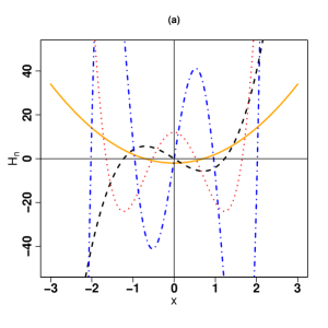
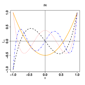
  Figure 4.2: Graph of (a): Hermite and (b): Legendre polynomials of orders $n=2$ (solid orange line), $n=3$ (dashed black line), $n=4$ (dotted red line), and $n=5$ (dotted-dashed blue line).

  Figure 4.2 displays the graph of Hermite and Legendre polynomials of orders $n=2,3,4,5$.

• Laguerre polynomial: The Laguerre polynomial of degree $n$, shown by ${\cal{L}}_{n}(x)$, is orthogonal with respect to weight function $w(x)=\exp\{-x\}$. This means that

  $$\langle{\cal{L}}_{n},{\cal{L}}_{m}\rangle=\int_{0}^{\infty}{\cal{L}}_{n}(x){\cal{L}}_{m}(x)\exp\{-x\}dx={\cal{D}}_{m,n}.$$ (4.18)

  This class of orthogonal polynomials is solution of the differential equation

  $$x\frac{d^{2}{\cal{L}}_{n}(x)}{dx^{2}}+(1-x)\frac{d{\cal{L}}_{n}(x)}{dx}+n{\cal{L}}_{n}(x)=0,$$ (4.19)

  whose solution becomes

  $${\cal{L}}_{n}(x)=\Gamma(n+1)\sum_{i=0}^{n}\frac{(-1)^{i}x^{i}}{\Gamma(n-i+1)\bigl{[}\Gamma(i+1)]^{2}}.$$ (4.20)

  Using expression (4.20), the first six members of Laguerre polynomials are as follows.

  $${\cal{L}}_{0}(x) =1,$$

  $${\cal{L}}_{1}(x) =1-x,$$

  $${\cal{L}}_{2}(x) =\frac{x^{2}-4x+2}{2},$$

  $${\cal{L}}_{3}(x) =-\frac{x^{3}-9x^{2}+18x-6}{6},$$

  $${\cal{L}}_{4}(x) =\frac{x^{4}-16x^{3}+72x^{2}-96x+24}{24},$$

  $${\cal{L}}_{5}(x) =\frac{-x^{5}+25x^{4}-200x^{3}+600x^{2}-600x+120}{120}.$$

Table 4.1 shows a list of most commonly used orthogonal polynomials in statistics.

Table 4.1: The most commonly used orthogonal polynomials.

$P_{n}(\cdot)$	symbol	${\text{C}_{n}}$	$[a,b]$	$w(x)$
$\begin{matrix}{\text{Chebyshev}}\\ {\text{(first kind)}}\end{matrix}$	$T_{1,n}$	$\begin{cases}\pi&\mathrm{if}\ n=0,\\ \frac{\pi}{2}&\mathrm{if}\ n\neq 0\end{cases}$	$(-1,1)$	$\bigl{(}1-x^{2}\bigr{)}^{-\frac{1}{2}}$
$\begin{matrix}{\text{Chebyshev}}\\ {\text{(second kind)}}\end{matrix}$	$T_{2,n}$	$\frac{\pi}{2}$	$[-1,1]$	$\bigl{(}1-x^{2}\bigr{)}^{\frac{1}{2}}$
$\begin{matrix}{\text{Generalized}}\\ {\text{Laguerre}}\end{matrix}$	${\cal{L}}_{n}^{\alpha}$	$\frac{\Gamma(n+\alpha+1)}{\Gamma(n+1)}$	$[0,\infty)$	$\begin{matrix}x^{\alpha}\exp\bigl{\{}-x\bigr{\}},\\ \alpha>-1\end{matrix}$
Hermite	$H_{n}$	$2^{n}\sqrt{\pi}\Gamma(n+1)$	$(-\infty,\infty)$	$\exp\{-{x^{2}}{}\}$
Jacobi	$J_{n}^{\alpha,\beta}$	$\begin{matrix}\frac{2^{\alpha+\beta+1}}{2n+\alpha+\beta+1}\times\\ \frac{\Gamma(n+\alpha+1)\Gamma(n+\beta+1)}{\Gamma(n+\alpha+\beta+1)\Gamma(n+1)}\end{matrix}$	$(-1,1)$	$\begin{matrix}(1-x)^{\alpha}(1+x)^{\beta}\mathrm{,}\\ \alpha,\beta>-1\end{matrix}$
Laguerre	${\cal{L}}_{n}$	1	$[0,\infty)$	$\exp\bigl{\{}-x\bigr{\}}$
Legendre	$L_{n}$	$\frac{2}{2n+1}$	$[-1,1]$	1

There are different types of the Gaussian quadrature rules have been developed in the literature for approximating the integral (4.21). Particular Gauss quadrature rule arises from particular choice of the interval and the form of the weight function $w(x)$. For example, the Gauss-Legendre quadrature rule is applied when $[a,b]=[-1,1]$ and $w(x)=1$, and so is employed for approximating integral of the form

$$\int_{-1}^{1}f(x)dx.$$

Moreover, for approximating integral of the form

$$\int_{0}^{\infty}\exp\{-x\}f(x)dx,$$

we may use the Gauss-Laguerre quadrature rule since as it is seen the range of integral is $[a,b]=[0,\infty)$ and $w(x)=\exp\{-x\}$, and finally, a $k$-point Gauss-Chebyshev rule is useful when $[a,b]=[-1,1]$. The bounds of integral (4.21) can be changed from $(a,b)$ to $[-1,1]$ through a simple transformation when $a\neq-1$ and $b\neq 1$. For integrand of the form $w(x)f(x)$, in which $w(x)$ is given in Table 4.1, an orthogonal polynomial up to degree $k+1$ is fitted to integrand $w(x)f(x)$ that intercepts integrand $w(x)f(x)$ at $k$ nodes $\{x_{n}\}_{n=1}^{k}$. Once we have found $k$ pairs of nodes and associated weights, shown by $\{\bigl{(}x_{n},\omega_{n}\bigr{)}\}_{n=1}^{k}$, the integral can be approximated based on a $k$-point Gaussian quadrature rule as

$$\int_{a}^{b}w(x)f(x)dx\approx\sum_{n=1}^{k}\omega_{n}f\bigl{(}x_{n}\bigr{)}.$$ (4.21)

The nodes and weighs for Gauss-Chebyshev quadrature are determined simply. The class ${{T}}_{1,n}(\cdot)$ and ${{T}}_{2,n}(\cdot)$ of orthogonal polynomials are given by

$$\begin{cases}{{T}}_{1,n}(x)=\cos\bigl{(}n\theta\bigr{)},&{\text{for first kind,}}\\ {{T}}_{2,n}(x)=\frac{\sin\bigl{(}(n+1)\theta\bigr{)}}{\sin(\theta)},&{\text{for second kind,}}\end{cases}$$ (4.22)

where $x=\cos(\theta)$ for $\theta\in[0,\pi]$ (Rivlin, 2020). These two classes of orthogonal polynomials admit the recurrence relation

$${{T}}_{1,n+1}(x)=2x{{T}}_{1,n}(x)-{{T}}_{1,n-1}(x),\leavevmode\nobreak\ \mathrm{for}\leavevmode\nobreak\ n\geq 1,$$ (4.23)

where ${T}_{1,0}(x)=1$ and ${T}_{1,1}(x)=x$. The nodes are given by

$$\begin{cases}x_{n}=\cos\Bigl{(}\frac{2n-1}{2k}\pi\Bigr{)},&{\text{for first kind,}}\\ x_{n}=\cos\Bigl{(}\frac{n}{k+1}\pi\Bigr{)},&{\text{for second kind,}}\end{cases}$$ (4.24)

where $n=1,\cdots,k$. The pertaining weights for the first and second kinds are the same and distributed uniformly, that is $\omega_{n}=\pi/k$, for $n=1,\cdots,k$. The Gaussian quadrature rules based on the other orthogonal polynomials are determined through the Golub-Welsch algorithm (Golub and Welsch, 1969) as follows.

4.0.2 Golub-Welsch algorithm

The fundamental Gaussian quadrature theorem states that the nodes $x_{i}$s are the roots of the orthogonal polynomial. It can be shown that each orthogonal polynomial of degree $k$ has distinct real roots on interval $[a,b]$ (Shen et al., 2011, pp. 53). There are two simple methods for computing the roots of orthogonal polynomial (Shen et al., 2011, pp. 55). Except for the Chebyshev case, the roots of other orthogonal polynomials may be obtained trough the eigenvalue or iterative method. In what follows, we describe briefly the eigenvalue method or Golub-Welsch algorithm, see (Shen et al., 2011, pp. 55).

• nodes: Let $P_{n}(x)$ denote the orthogonal polynomial. It can be seen that the orthogonal polynomials given on Table 4.1 admits the recurrence formula as (Shen et al., 2011, Theorem 3.1):

  $$xP_{n}(x)=a_{n}P_{n+1}(x)+b_{n}P_{n}(x)+c_{n}P_{n-1}(x),$$ (4.25)

  for $c_{0}P_{-1}(x)=0$. The zeros of the orthogonal polynomial $P_{n}(x)$ are eigenvalues of symmetric threediagonal matrix $A$ given by (Gil et al., 2007):

  $$A=\left(\begin{matrix}b_{0}&\sqrt{a_{0}c_{1}}&&&\\ \sqrt{a_{0}c_{1}}&b_{1}&\sqrt{a_{1}c_{2}}&&\\ &\sqrt{a_{1}c_{2}}&b_{2}&&\\ &&&\ddots&\sqrt{a_{k-2}c_{k-1}}\\ &&&\sqrt{a_{k-2}c_{k-1}}\ &b_{k-1}\end{matrix}\right),$$ (4.26)

  where

  $$\alpha_{0}P_{-1}(x)=0,fori\geq 0.$$

  The eigenvalues ${e}_{1},\cdots,{e}_{k}$ of matrix $A$ are also nodes of the Gaussian quadrature rule, that is $e_{n}=x_{n}$, for $n=1,\cdots,k$.

• weight: Once we have computed the eigenvalues of $A$ in (4.26), the $n$th eight $\omega_{n}$ is obtained as

  $$\omega_{n}=\mu_{0}\frac{\bigl{(}\bm{v}_{n}[1]\bigr{)}^{2}}{\lVert\bm{v}_{n}\rVert},$$ (4.27)

  in which

  $$\mu_{0}=\int_{a}^{b}w(x)dx,$$

  $\lVert\cdot\rVert$ denotes the Euclidean norm, $\{\bm{v}_{1},\cdots,\bm{v}_{k}\}$ are the eigenvectors correspond to $\{{e}_{1},\cdots,{e}_{k}\}$, and $\bm{v}_{n}[1]$ is the first element of eigenvector $\bm{v}_{n}$.

In what follows, we compute the Gaussian quadrature rule for orthogonal polynomials presented in Table 4.1.

• nodes and weighs for generalized Laguerre polynomial: The class ${\cal{L}}^{\alpha}_{n}(\cdot)$ of orthogonal polynomials admits the recurrence relation

  $$(n+1){\cal{L}}^{\alpha}_{n+1}(x)=(2n+\alpha+1-x){\cal{L}}^{\alpha}_{n}(x)-(n+\alpha){\cal{L}}^{\alpha}_{n-1}(x),$$ (4.28)

  where ${\cal{L}}^{\alpha}_{0}(x)=1$. Comparing the recurrence relations given in (4.25) and (4.28), we obtain $b_{n}=0$, for $n=0,1,2,\cdots$, and

  $$\begin{cases}a_{n}=-(n+1)\leavevmode\nobreak\ {\text{and}}\leavevmode\nobreak\ b_{n}=(2n+\alpha+1),&{\text{if}}\leavevmode\nobreak\ n\geq 0,\\ c_{n}=-(n+\alpha),&{\text{if}}\leavevmode\nobreak\ n\geq 1.\end{cases}$$ (4.29)

  In this case, matrix $A$ in (4.26) can be reconstructed by using the constants $a_{n}$, $b_{n}$, and $c_{n}$ provided in (4.29) for computing eigenvalues of the reconstructed matrix $A$ as the nodes. For computing weights, it follows from Table 4.1 that

  $$\mu_{0}=\int_{a}^{b}w(x)dx=\int_{0}^{\infty}x^{\alpha}\exp\{-x\}dx=\Gamma(\alpha+1).$$

  Hence the weights $\omega_{n}$ (for $n=1,\cdots,k$) are obtained by considering $\mu_{0}=\Gamma(\alpha+1)$ in the RHS of (4.27) in which $\bm{v}_{n}$ (for $n=1,\cdots,k$) is the eigenvector corresponds to $i$th eigenvalue of matrix $A$ constructed based on information given by (4.29).

• nodes and weighs for Hermite polynomial: The class ${{H}}^{\alpha}_{n}(\cdot)$ of orthogonal polynomials admits the recurrence relation given by (4.17) for $n\geq 1$. Comparing the recurrence relations given in (4.25) and (4.17), we obtain

  $$\begin{cases}a_{n}=\frac{1}{2}\leavevmode\nobreak\ {\text{and}}\leavevmode\nobreak\ b_{n}=0,\leavevmode\nobreak\ \leavevmode\nobreak\ &{\text{if}}\ n\geq 0,\\ c_{n}=n,\leavevmode\nobreak\ \leavevmode\nobreak\ &{\text{if}}\ n\geq 1.\end{cases}$$ (4.30)

  In this case, matrix $A$ in (4.26) can be reconstructed by using the constants $a_{n}$, $b_{n}$, and $c_{n}$ provided in (4.30) for computing eigenvalues of the reconstructed matrix $A$ as the nodes. For computing weights, it follows from Table 4.1 that

  $$\mu_{0}=\int_{a}^{b}w(x)dx=\int_{-\infty}^{\infty}\exp\{-{x^{2}}{}\}dx=\sqrt{2\pi}.$$

  Hence the weights $\omega_{n}$ (for $n=1,\cdots,k$) are obtained by considering $\mu_{0}=\sqrt{\pi}$ in the RHS of (4.27) in which $\bm{v}_{n}$ (for $n=1,\cdots,k$) is the eigenvector corresponds to $i$th eigenvalue of matrix $A$ constructed based on information given by (4.30).

• nodes and weighs for Jacobi polynomial: The class $J^{\alpha,\beta}_{i}(\cdot)$ of orthogonal polynomials admits the recurrence relation

  $$J^{\alpha,\beta}_{n+1}(x)=\bigl{(}xa^{\alpha,\beta}_{n}-b^{\alpha,\beta}_{n}\bigr{)}J^{\alpha,\beta}_{n}(x)-c^{\alpha,\beta}_{n}J^{\alpha,\beta}_{n-1}(x),$$ (4.31)

  with $J^{\alpha,\beta}_{0}(x)=1$ and $J^{\alpha,\beta}_{1}(x)=x(\alpha+\beta+2)/2+(\alpha-\beta)/2$, for $n=1,2,\cdots$. Furthermore,

  $$a^{\alpha,\beta}_{n} =\frac{(2n+\alpha+\beta+1)(2n+\alpha+\beta+2)}{2(n+1)(n+\alpha+\beta+1)},$$

  $$b^{\alpha,\beta}_{n} =\frac{(\beta^{2}-\alpha^{2})(2n+\alpha+\beta+1)}{2(n+1)(n+\alpha+\beta+1)(2n+\alpha+\beta)},$$

  $$c^{\alpha,\beta}_{n} =\frac{(n+\alpha)(n+\beta)(2n+\alpha+\beta+2)}{(n+1)(n+\alpha+\beta+1)(2n+\alpha+\beta)}.$$ (4.32)

  Rearranging the RHS of (4.31) and comparing it with the recurrence relation given in (4.25), we obtain

  $$\begin{cases}a_{0}=\frac{2}{\alpha+\beta+2}\leavevmode\nobreak\ {\text{and}}\leavevmode\nobreak\ b_{0}=\frac{\beta-\alpha}{\alpha+\beta+2},&{\text{if}}\leavevmode\nobreak\ \ n=0,\\ a_{n}=\frac{2(n+1)(n+\alpha+\beta+1)}{(2n+\alpha+\beta+1)(2n+\alpha+\beta+2)},&{\text{if}}\leavevmode\nobreak\ \ n\geq 1,\\ b_{n}=\frac{\beta^{2}-\alpha^{2}}{(2n+\alpha+\beta)(2n+\alpha+\beta+2)},&{\text{if}}\leavevmode\nobreak\ \ n\geq 1,\\ c_{n}=\frac{2(n+\alpha)(n+\beta)}{(2n+\alpha+\beta)(2n+\alpha+\beta+1)},&{\text{if}}\leavevmode\nobreak\ \ n\geq 1.\end{cases}$$ (4.33)

  In this case, matrix $A$ in (4.26) can be reconstructed by using the constants $a_{n}$, $b_{n}$, and $c_{n}$ provided in (4.33). As before, the nodes are eigenvalues of the reconstructed matrix $A$ and for computing weights, it follows from Table 4.1 that

  $$\mu_{0}=\int_{a}^{b}w(x)dx=\int_{-1}^{1}(1-x)^{\alpha}(1+x)^{\beta}dx=\frac{2^{\alpha+\beta+1}\Gamma(\alpha+1)\Gamma(\beta+1)}{\Gamma(\alpha+\beta+1)}.$$

  Hence the weights $\omega_{n}$ (for $n=1,\cdots,k$) are obtained by considering $\mu_{0}=2$ in the RHS of (4.27) in which $\bm{v}_{n}$ (for $n=1,\cdots,k$) is the eigenvector corresponds to $n$th eigenvalue of matrix $A$ constructed based on information given by (4.33).

• nodes and weighs for Legendre polynomial: The class $L_{n}(\cdot)$ of orthogonal polynomials admits the recurrence relation

  $$xL_{n}(x)=\frac{n+1}{2n+1}L_{n+1}(x)+\frac{n}{2n+1}L_{n-1}(x),$$ (4.34)

  with $L_{0}(x)=1$ and $L_{1}(x)=x$, for $n=1,2,\cdots$. Comparing the recurrence relations given in (4.25) and (4.34), we obtain $b_{n}=0$, for $n=0,1,2,\cdots$, and

  $$\begin{cases}a_{n}=\frac{n+1}{2n+1},\leavevmode\nobreak\ &{\text{if}}\ n\geq 0,\\ c_{n}=\frac{n}{2n+1},\leavevmode\nobreak\ &{\text{if}}\ n\geq 1.\end{cases}$$ (4.35)

  In this case, matrix $A$ in (4.26) can be reconstructed by setting $\sqrt{a_{n-1}c_{n}}=n/\sqrt{4n^{2}-1}$ (for $n=1,\cdots,k$) in the RHS of (4.26). The nodes are eigenvalues of the reconstructed matrix $A$. For computing weights, it follows from Table 4.1 that

  $$\mu_{0}=\int_{a}^{b}w(x)dx=\int_{-1}^{1}dx=2.$$

  Hence the weights $\omega_{n}$ (for $n=1,\cdots,k$) are obtained by considering $\mu_{0}=2$ in the RHS of (4.27) in which $\bm{v}_{n}$ (for $n=1,\cdots,k$) is the eigenvector corresponds to $n$th eigenvalue of matrix $A$ constructed based on information given by (4.35).

It should be noted that the accuracy of a Gaussian quadrature depends on the structure of the orthogonal polynomial. In general, if $f(x)$ in (4.21) has continuous derivatives of order $2k$, then the error in approximating integral (4.21) becomes (Kahaner et al., 1989):

$${\text{Error}}=\int_{a}^{b}w(x)f(x)dx-\sum_{i=1}^{k}\omega_{i}f(x_{i})=\frac{f^{(2k)}(\eta)}{\Gamma(2k+1)}\int_{a}^{b}w(x)P^{2}_{k}(x)dx,$$

where $f^{(2k)}(\eta)$ denotes the $(2k)$th derivative of $f(x)$ for some $a<\eta<b$. In special case, when $w(x)=1$, we have

$${\text{Error}}=\frac{(b-a)^{2k+1}\bigl{[}\Gamma(k+1)\bigr{]}^{4}}{(2k+1)\bigl{[}\Gamma(2k+1)\bigr{]}^{3}}f^{(2k)}(\eta).$$

As a useful criterion, the goodness of approximation $\hat{I}$ for integral $I$ is reflected by absolute relative error (ARE) criteria defined as

$${\text{ARE}}=\Bigl{|}\frac{I-\hat{I}}{I}\Bigr{|}.$$ (4.36)

The following R function quad_rule is provided to compute the nodes and weights for implementing the Gaussian quadrature rules discussed earlier. We note that the argument type includes: CH1 (for Chebyshev of first kind), CH2 (for Chebyshev of second kind), HE (for Hermite), GL (for generalized Laguerre), JA (for Jacobi), and LE (for Legendre). Furthermore, arguments alpha and beta are parameters of Gaussian quadrature based on generalized Laguerre or Jacobi orthogonal polynomials.

⬇

1R> quad_rule <- function(n, type = "HE", alpha = 0, beta = 0)

2+{

3+ if (any(c(alpha,beta) <= -1))stop("␣alpha␣and␣beta␣must␣be␣greater␣than␣-1.")

4+ A <- diag(0, n)

5+ if ( type == "CH1" )

6+ {

7+ ia <- 1:n

8+ node <- cos( (2*ia - 1)/(2*n)*pi )

9+ weight <- pi/n

10+ }

11+ if ( type == "CH2" )

12+ {

13+ ia <- 1:n

14+ node <- cos( ia/(n + 1)*pi )

15+ weight <- pi/n

16+ }

17+ if ( type == "HE" )

18+ {

19+ a_nc_n <- 1:(n - 1)/2

20+ A[row(A) - col(A) == 1] <- A[row(A) - col(A) == -1] <- sqrt( a_nc_n )

21+ A_eigen <- eigen(A)

22+ node <- A_eigen$values

23+ weight <- sqrt(pi)*( A_eigen$vector[1, ] )^2

24+ }

25+ if ( type == "GL" )

26+ {

27+ ib <- seq(0, n - 1)

28+ b_n <- 2*ib + alpha + 1

29+ ia <- seq(0, n - 2)

30+ diag(A) <- b_n

31+ A[row(A) - col(A) == 1] <- A[row(A) - col(A) == -1] <-

32+ sqrt( (ia + 1)*(ia + 1 + alpha) )

33+ A_eigen <- eigen(A)

34+ node <- A_eigen$values

35+ weight <- gamma(alpha + 1)*( A_eigen$vector[1, ] )^2

36+ }

37+ if ( type == "JA" )

38+ {

39+ ib <- seq(1, n - 1)

40+ b_n <- (beta^2 - alpha^2)/( (2*ib + alpha + beta)*

41+ (2*ib + alpha + beta + 2) )

42+ ia <- seq(1, n - 2)

43+ a_n <- 2*(ia + 1)*(ia + alpha + beta + 1)/( (2*ia + alpha + beta + 1)*

44+ (2*ia + alpha + beta + 2) )

45+ ic <- ia + 1

46+ c_n <- 2*(ic + alpha)*(ic + beta )/( (2*ic + alpha + beta)*

47+ (2*ic + alpha + beta + 1) )

48+ diag(A) <- c(0, b_n )

49+ A[row(A) - col(A) == 1] <- A[row(A) - col(A) == -1] <- c(0, sqrt( a_n*c_n ) )

50+ A[1, 1] <- (beta - alpha)/( alpha + beta + 2 )

51+ A[1, 2] <- sqrt( 4*(1 + alpha)*(1 + beta )/

52+ ( (2 + alpha + beta)^2*(3 + alpha + beta) ) )

53+ A[2, 1] <- A[1, 2]

54+ A_eigen <- eigen(A)

55+ node <- A_eigen$values

56+ weight <- 2^(alpha + beta + 1)*(alpha + beta + 1)*

57+ beta(alpha + 1, beta + 1)*( A_eigen$vector[1, ] )^2

58+ }

59+ if ( type == "LE" )

60+ {

61+ ia <- seq(0, n - 2)

62+ a_n <- (ia + 1)/(2*ia + 1)

63+ ic <- ia + 1

64+ c_n <- ic/(2*ic + 1)

65+ A[row(A) - col(A) == 1] <- A[row(A) - col(A) == -1] <- sqrt( a_n*c_n )

66+ A_eigen <- eigen(A)

67+ node <- A_eigen$values

68+ weight <- 2*( A_eigen$vector[1, ] )^2

69+ }

70+ ls <- list( "node" = node , "weight" = weight)

71+ return(ls)

72+}

Example 10 Let’s to approximate integral (4.12) of Example 4 through the Gaussian-Legendre rule. To this end, first, we need to convert the range of integration from $[0,3]$ to $[-1,1]$. Using a change of variable $z=2u/3-1$ it turns out that

$$I=\int_{0}^{3}x\exp\{-x\}dx= \frac{9}{4}\exp\Bigl{\{}-\frac{3}{2}\Bigr{\}}\int_{-1}^{1}(z+1)\exp\Bigl{\{}-\frac{3}{2}z\Bigr{\}}dz$$

$$= \frac{9}{4}\exp\Bigl{\{}-\frac{3}{2}\Bigr{\}}\int_{-1}^{1}w(z)f(z)dz,$$ (4.37)

where $w(z)=1$ and $f(z)=(z+1)\exp\bigl{\{}-3z/2\bigr{\}}$. Hence, the sequence of nodes and weights can be computed using function quad_rule, when type=”LE”. Computing the sequence $\{x_{i},\omega_{i}\}_{i=1}^{k}$, we can write

$$I\approx\frac{9}{4}\exp\Bigl{\{}-\frac{3}{2}\Bigr{\}}\sum_{i=1}^{k}\omega_{i}\times\bigl{(}x_{i}+1\bigr{)}\exp\Bigl{\{}-\frac{3}{2}x_{i}\Bigr{\}}.$$ (4.38)

The pertaining AREs for $k=2,3,5$ and 10 are 4.58e-02, 1.50e-03 1.75e-07, and 3.18e-15, respectively. We remind that the general quadrature rule applied in Example 4 yields 0.83755 with ${\text{ARE}}=0.045$. Evidently, he Gaussian quadrature shows superior performance with ${\text{ARE}}=0.045$ just by adding one more node.

Example 11 Suppose we are interested in approximating

$$I(p)=\int_{0}^{\infty}x^{p}\log x\exp\bigl{\{}-x\bigr{\}}dx,$$ (4.39)

where $p>0$. Since the range of integrand $I$ is $(0,\infty)$ and involves the term $\exp\{-x\}$, using class ${\cal{L}}^{p}_{k}$ of orthogonal polynomials, a Gaussian quadrature rule is applied for approximating $I(p)$ for different settings of $k$ and $p$. To this end, we compute the sequence of nodes and weights using function quad_rule, when type=”GL” and alpha=$p$. Computing sequence $\{x_{i},\omega_{i}\}_{i=1}^{k}$, we approximate integral $I(p)$ as follows.

$$I(p)\approx\sum_{i=1}^{k}\omega_{i}\times\bigl{(}x_{i}\bigr{)}^{p}\log x_{i}.$$ (4.40)

Table 4.2 shows the ARE results for computing integral $I(p)$ in (4.39). It turns out from Table 4.2 that for larger $p$, smaller $k$ provides the accuracy at desired level. Table 4.2: The ARE for approximating integral in (4.39). ARE p Exact value of $I(p)$ $k=5$ $k=10$ $k=15$ $k=20$ 0 -0.5772156 0.214375 0.108274 7.24e-02 5.44e-02 1 0.42278433 4.50e-01 0.012404 5.70e-03 3.26e-03 2 1.84556867 5.69e-03 9.12e-04 2.96e-04 1.30e-04 3 7.53670601 1.53e-03 1.51e-04 3.54e-05 1.22e-05 4 36.1468240 5.64e-04 3.55e-05 6.14e-06 1.68e-06

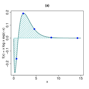
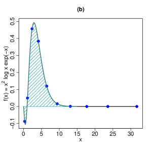
Figure 4.3: Graph of integrand (4.39). (a): $p=1$ and $k=5$, (b): $p=2$ and $k=10$. Figure 4.3 shows the integrand of integral $I(p)$ in (4.39) on which x-coordinates of bullets are the position of the nodes.

Example 12 Suppose we are interested in approximating

$$I(z,\alpha)=\frac{1}{2\pi}\int_{-\infty}^{\infty}\exp\bigl{\{}-u^{\alpha}\bigr{\}}\cos(zu)du,$$ (4.41)

where $0<\alpha\leq 2$. In fact, integral $I(z,\alpha)$ is the PDF of symmetric standard $\alpha$-stable distribution at point $z$ (Nolan, 2020). For $\alpha=2$, each standard symmetric $\alpha$-stable distribution turns into a zero-mean Gaussian distribution with scale $1/\sqrt{2}$. Hence, we have $I(z,2)={\cal{N}}(z|0,1/2)$. Herein, using a Gauss-Hermite rule, we proceed to approximate integral $I(z,\alpha)$. Table 4.3 shows the ARE for different settings of $k$ and $z$. As it is seen, the ARE for large $z$ decreases and a larger $k$ needs to provide the accuracy of desired level. Table 4.3: The ARE for approximating integral in (4.41) using Gauss-Hermite rule. ARE z Exact value of $I(z,2)$ $k=5$ $k=10$ $k=15$ $k=20$ 0 0.28209479 1.96e-16 1.96e-16 1.96e-16 5.90e-16 1 0.21969564 1.18e-06 2.65e-15 8.84e-16 1.51e-15 2 0.10377687 1.80e-03 2.56e-09 3.61e-15 5.08e-15 3 0.02973257 2.02e-01 1.63e-05 9.84e-11 1.08e-14 4 0.00516674 9.18174 1.27e-02 1.35e-06 2.64e-11 5 0.00054457 284.672 3.568332 3.47e-03 6.29e-07 Figure 4.4 displays the pertaining integrand on which x-coordinates of bullets are the position of the nodes that are symmetrically distributed around origin. It it worth to note that integrand in (4.41) is an oscillatory function and when $z$ is large the number of oscillations is large (Nolan, 2020, pp. 68).

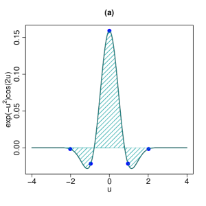
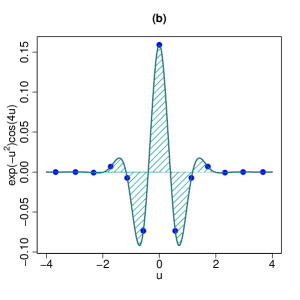
Figure 4.4: Graph of integrand (4.41) for (a): $z=2$ and $k=5$, (b):$z=4$ and $k=15$.

Chapter 5 Moments of truncated distributions

Truncated distribution is widely used in different fields of statistics such as, survival analysis, regression analysis, and model-based clustering. We write ${\cal{X}}$ to denote the truncated version of random variable $X$ on $(a,b)$. The random variable may take any value on real line, but ${\cal{X}}$ just takes values on $(a,b)$. The latter is known as the doubly truncated of $X$. There are two other types of truncated random variable including the left truncated random variables. If ${\cal{X}}$ is defined on $(b,\infty)$, then we may say that ${\cal{X}}$ is the left truncated version of $X$ at $b$. Likewise, if ${\cal{X}}$ is defined on $(-\infty,a)$, then we may say that ${\cal{X}}$ is the right truncated version of $X$ at $a$. The PDF of random variable ${\cal{X}}$ truncated on $(a,b)$ is given by

$$\frac{f(x)}{\int_{a}^{b}f(u)du},$$ (5.1)

where $-\infty<a<x<b<\infty$. Each doubly random variable ${\cal{X}}$ is in fact a conditional version of random variable $X$. In other words

$${{\cal{X}}}_{a,b}=X\big{|}X\in(a,b).$$ (5.2)

Let $F(\cdot)$ denotes the CDF of random variable $X$. Elementary calculations show that the CDF of ${{\cal{X}}}$ can be represented in terms of $F(\cdot)$ as follows.

$$\frac{F(x)-F(a)}{F(b)-F(a)},\leavevmode\nobreak\ \leavevmode\nobreak\ -\infty<a<x<b<\infty.$$ (5.3)

Hence, in univariate case, the $m$th moment of truncated random variable $X$ on $(a,b)$, for $m=1,2,3,\cdots$ is

$$\Omega^{m}=E\bigl{(}X^{m}\big{|}a<X<b\bigr{)}=\frac{\int_{a}^{b}u^{m}f(u)du}{F(b)-F(a)},\leavevmode\nobreak\ -\infty<a<x<b<\infty.$$ (5.4)

In multivariate case, the PDF of truncated random vector $\bm{X}$ on hyper-cube $(\bm{a},\bm{b})\subset\mathbb{R}^{p}$ with lower bound $\bm{a}=(a_{1},\cdots,a_{p})^{\top}$ and upper bound $\bm{b}=(b_{1},\cdots,b_{p})^{\top}$ is given by

$$\frac{f(\bm{x})}{\int_{\bm{a}}^{\bm{b}}f(\bm{u})d\bm{u}}=\frac{f(\bm{x})}{F(\bm{b})-F(\bm{a})},$$ (5.5)

where $\bm{a}<\bm{x}<\bm{b}$ and $F(\cdot)$ is the CDF of $\bm{X}$. So, the first and second moments of truncated random vector $\bm{X}$, respectively, are

$$\bm{\Omega}= E\bigl{(}\bm{X}\big{|}\bm{a}<\bm{X}<\bm{b}\bigr{)}=E\bigl{(}\bm{X}\big{|}a_{1}<X_{1}<b_{1},\cdots,a_{p}<X_{p}<b_{p}\bigr{)},$$

$$\bm{\Omega}^{2}= E\bigl{(}\bm{X}\bm{X}^{\top}\big{|}\bm{a}<\bm{X}<\bm{b}\bigr{)}=E\bigl{(}\bm{X}\bm{X}^{\top}\big{|}a_{1}<X_{1}<b_{1},\cdots,a_{p}<X_{p}<b_{p}\bigr{)}.$$

Herein, the concern of study mainly is devoted to computing the first and second moments given by since these quantities have received more attention than other moments in practice. If $\bm{X}\sim f(\cdot)$, by definition, the first moment of $\bm{X}$ is computed as

$$\bm{\Omega}= \frac{1}{F(\bm{b})-F(\bm{a})}\int_{\bm{a}}^{\bm{b}}\bm{u}f(\bm{u})d\bm{u}.$$ (5.6)

The Monte Carlo approximation of $\bm{\Omega}$ can be obtained by considering the instrumental distribution with PDFs $f(\cdot)/\bigl{[}F(a)-F(b)\bigr{]}$. Here, we can use the rejection approach for simulating from truncated random variable as follows. Suppose, $x_{1},\cdots,x_{N}$, for sufficiently large $N$, are realizations from instrumental with PDF $f_{1}$, the Monte Carlo approximation of $\bm{\Omega}$ is obtained as

$$\hat{\bm{\Omega}}=\frac{1}{N}\sum_{i=1}^{N}f_{1}\bigl{(}x_{i}\bigr{)}.$$ (5.7)

The pseudo code for sampling from $f(\cdot)/\bigl{[}F(a)-F(b)\bigr{]}$ is given as follows.

1. Read ${a},{b}$, and $N$;

2. Set $j=0$ and ${y}=0$;

3. Simulate ${x}\sim f(\cdot)$

4. If $a<x<b$, then accept ${x}$ as a generation from $f(\cdot)/\bigl{[}F(a)-F(b)\bigr{]}$, set ${y}={y}+x$ and $j=j+1$;

5. If $j=N$, then go to the next step, otherwise return to step 2;

6. Approximate $\Omega$ as $\hat{\Omega}=y/N$;

7. End.

The focus of this chapter is placed on compute the the first and second moments of truncated Gaussian distribution in univariate and multivariate cases. Herein, we proceed to compute the exact values of first and second moments of the truncated univariate and multivariate Gaussian distributions.

5.1 Moments of truncated Gaussian distribution in univariate case

For simplicity, we use generic symbols $\phi\bigl{(}{x}\big{|}{\mu},\sigma^{2}\bigr{)}$ and ${\Phi}\bigl{(}{x}\big{|}{\mu},\sigma^{2}\bigr{)}$ to show, accordingly, the PDF and CDF of a Gaussian distribution at point ${x}$ for which ${\mu}$ and $\sigma$ are the location and scale parameters, respectively. We further write ${X}\sim{\cal{N}}({\mu},\sigma^{2})$ to show that random variable ${X}$ follows a Gaussian distribution with location parameter ${\mu}$ and variance $\sigma^{2}$. The corresponding truncated family on $(a,b)$ is represented by $t{\cal{N}}\bigl{(}{\mu},\sigma^{2},a,b\bigr{)}$.

5.1.1 First two moments of truncated Gaussian distribution

Let $X\sim{\cal{N}}\bigl{(}\mu,\sigma^{2}\bigr{)}$. By definition, from (5.4) for $m=1$, it follows that

$$\Omega=E\bigl{(}X\big{|}a<X<b\bigr{)}=\frac{1}{\Phi(b|\mu,\sigma^{2})-\Phi(a|\mu,\sigma^{2})}\int_{a}^{b}x\times\phi(x|\mu,\sigma^{2})dx.$$ (5.8)

It is easy to check that

$$\frac{\partial}{\partial\mu}\phi(x|\mu,\sigma^{2})= \Bigl{(}\frac{x-\mu}{\sigma^{2}}\Bigr{)}\phi(x|\mu,\sigma^{2}).$$ (5.9)

Integrating both sides of (5.9) and dividing by $P_{G}=\Phi(b|\mu,\sigma^{2})-\Phi(a|\mu,\sigma^{2})$ yields

$$\frac{1}{P_{G}}\int_{a}^{b}\frac{\partial}{\partial\mu}\phi(x|\mu,\sigma^{2})dx=\frac{\Omega}{\sigma^{2}}-\frac{\mu}{\sigma^{2}}.$$

It follows that

$$\Omega =\mu+\frac{\sigma^{2}}{P_{G}}\frac{\partial}{\partial\mu}\int_{a-\mu}^{b-\mu}\phi(u|0,\sigma^{2})du$$

$$=\mu+\frac{\sigma^{2}}{P_{G}}\Bigl{[}\phi(a|\mu,\sigma^{2})-\phi(b|\mu,\sigma^{2})\Bigr{]}.$$

Hence,

$$\Omega=E\bigl{(}X\big{|}a<X<b\bigr{)}=\mu+\sigma^{2}\frac{\phi(a|\mu,\sigma^{2})-\phi(b|\mu,\sigma^{2})}{\Phi(b|\mu,\sigma^{2})-\Phi(a|\mu,\sigma^{2})}.$$ (5.10)

By definition, from (5.4) for $m=2$, it follows that

$$\Omega^{2}=E\bigl{(}X^{2}\big{|}a<X<b\bigr{)}=\frac{1}{P_{G}}\int_{a}^{b}x^{2}\phi(x|\mu,\sigma^{2})dx,$$

Taking the second order derivative from (5.9) with respect to $\mu$, we have

$$\frac{\partial^{2}}{\partial\mu^{2}}\phi(x|\mu,\sigma^{2})= \Bigl{(}\frac{x-\mu}{\sigma^{2}}\Bigr{)}^{2}\phi(x|\mu,\sigma^{2})-\frac{\phi(x|\mu,\sigma^{2})}{\sigma^{2}}.$$ (5.11)

Integrating both sides of (5.11), dividing by $P_{G}$, and then rearranging yields

$$\frac{1}{P_{G}}\frac{\partial^{2}}{\partial\mu^{2}}\int_{a-\mu}^{b-\mu}\phi(x|0,\sigma^{2})dx=\frac{1}{P_{G}}\int_{a}^{b}\Bigl{(}\frac{x-\mu}{\sigma^{2}}\Bigr{)}^{2}\phi(x|\mu,\sigma^{2})dx-\frac{1}{\sigma^{2}}.$$ (5.12)

It is easy to check that the LHS of (5.12) becomes

$$\frac{1}{P_{G}}\frac{\partial^{2}}{\partial\mu^{2}}\int_{a-\mu}^{b-\mu}\phi(x|0,\sigma^{2})dx=\frac{1}{P_{G}}\Bigl{[}\Bigl{(}\frac{a-\mu}{\sigma^{2}}\Bigr{)}\phi(a|\mu,\sigma^{2})-\Bigl{(}\frac{b-\mu}{\sigma^{2}}\Bigr{)}\phi(b|\mu,\sigma^{2})\Bigr{]},$$ (5.13)

and further

$$\frac{1}{P_{G}}\int_{a}^{b}\Bigl{(}\frac{x-\mu}{\sigma^{2}}\Bigr{)}^{2}\phi(x|\mu,\sigma^{2})dx= \frac{1}{\sigma^{2}}E\Bigl{[}\Bigl{(}\frac{X-\mu}{\sigma}\Bigr{)}^{2}\Big{|}a<X<b\Bigr{]}$$

$$= \frac{1}{\sigma^{4}}E\bigl{(}X^{2}\big{|}a<X<b\bigr{)}-2\frac{\mu}{\sigma^{4}}E\bigl{(}X\big{|}a<X<b\bigr{)}\Bigr{]}+\frac{\mu^{2}}{\sigma^{4}}.$$ (5.14)

Hence, substituting the RHS of (5.13) and (5.1.1) into (5.12) and rearranging, we obtain

$$\Omega^{2}=\sigma^{2}\frac{(a-\mu)\phi(a|\mu,\sigma^{2})-(b-\mu)\phi(b|\mu,\sigma^{2})}{\Phi(b|\mu,\sigma^{2})-\Phi(a|\mu,\sigma^{2})}+\sigma^{2}-\mu^{2}+2\mu\Omega.$$

In what follows R function Ex is given for computing the first and second moments of truncated univariate Gaussian distribution.

⬇

1R> Ex <- function(mu, sigma, a, b)

2+ {

3+ pb <- pnorm(b, mu, sigma)

4+ pa <- pnorm(a, mu, sigma)

5+ da <- dnorm(a, mu, sigma)

6+ db <- dnorm(b, mu, sigma)

7+ Omega <- mu + sigma^2*( da - db )/( pb - pa )

8+ P1 <- pnorm(b, mu, sigma) - pnorm(a, mu, sigma)

9+ ex <- mu + sigma^2*( da - db )/( pb - pa )

10+ Omega2 <- sigma^2*( (a-mu)*da - (b-mu)*db )/( pb - pa ) + sigma^2 -mu^2 + 2*mu*ex

11+ out2 <- list("Ex" = Omega, "Exx" = Omega2)

12+ return( out2 )

13+ }

5.2 First moment of truncated multivariate Gaussian distribution

For simplicity, we use generic symbols $\bm{\phi}_{p}\bigl{(}\bm{x}\big{|}\bm{\mu},\Sigma\bigr{)}$ and $\bm{\Phi}_{p}\bigl{(}\bm{x}\big{|}\bm{\mu},\Sigma\bigr{)}$ to denote, accordingly, the PDF and CDF of a $p$-dimensional Gaussian distribution at point $\bm{x}$ for which $\bm{\mu}$ and $\Sigma$ are the location and scale parameters, respectively. Also, we write $\bm{X}\sim{\cal{N}}_{p}\bigl{(}\bm{\mu},\Sigma\bigr{)}$ to indicate that random vector $\bm{X}$ follows a Gaussian distribution with location vector $\bm{\mu}$ and scale matrix $\Sigma$. The corresponding family of Gaussian distributions truncated on on hyper-cube $(\bm{a},\bm{b})\subset\mathbb{R}^{p}$ is shown by ${\cal{TN}}_{p}\bigl{(}\bm{\mu},\Sigma,\bm{a},\bm{b}\bigr{)}$. Furthermore, $\bm{\Omega}$ denotes the first moment of family ${\cal{TN}}_{p}\bigl{(}\bm{\mu},\Sigma,\bm{a},\bm{b}\bigr{)}$. Suppose $p$-dimensional random vector ${\bm{X}}=(X_{1},\cdots,X_{p})^{\top}$ follows ${\cal{N}}_{p}(\bm{\mu},\Sigma)$, we define the Mahalanobis distance as

$$\delta(\bm{x},\Sigma)=\bm{{{x}}}^{\top}{\Sigma}^{-1}\bm{x},$$ (5.15)

and

$$\bm{v}_{i}[x]=\bigl{(}{v}_{1},\cdots,{v}_{i-1},x,{v}_{i+1},\cdots,{v}_{p}\bigr{)},$$ (5.16)

$$\bm{v}[-i]=\bigl{(}{v}_{1},\cdots,{v}_{i-1},{v}_{i+1},\cdots,{v}_{p}\bigr{)},$$ (5.17)

in which $\bm{v}=\bigl{(}v_{1},v_{2},\cdots,v_{p}\bigr{)}^{\top}$ is a vector of real values. By definition, we can write

$$\bm{\Omega}= \frac{1}{{\cal{P}}_{G}}\int_{\bm{a}}^{\bm{b}}\bm{x}\times\bm{\phi}_{p}\bigl{(}\bm{x}\big{|}\bm{\mu},\Sigma\bigr{)}d\bm{x}$$

$$\frac{1}{{\bf{C}}_{G}{\cal{P}}_{G}}\int_{\bm{a}}^{\bm{b}}\bm{x}\exp\Bigl{\{}-\frac{\delta(\bm{x}-\bm{\mu},\Sigma)}{2}\Bigr{\}}d\bm{x}$$

$$= \frac{1}{{\bf{C}}_{G}{\cal{P}}_{G}}\int_{\bm{a}}^{\bm{b}}(\bm{x}-\bm{\mu})\exp\Bigl{\{}-\frac{\delta(\bm{x}-\bm{\mu},\Sigma)}{2}\Bigr{\}}d\bm{x}$$

$$+\frac{\bm{\mu}}{{\bf{C}}_{G}{\cal{P}}_{G}}\int_{\bm{a}}^{\bm{b}}\exp\Bigl{\{}-\frac{\delta(\bm{x}-\bm{\mu},\Sigma)}{2}\Bigr{\}}d\bm{x}$$

$$= \Sigma\bm{I}+\bm{\mu},$$ (5.18)

where ${\bf{C}}_{G}=(2\pi)^{p/2}|\Sigma|^{1/2}$, ${\cal{P}}_{G}=\bm{\Phi}_{p}\bigl{(}\bm{b}\big{|}\bm{\mu},{\Sigma}\bigr{)}-\bm{\Phi}_{p}\bigl{(}\bm{a}\big{|}\bm{\mu},{\Sigma}\bigr{)}$. Since

$$\frac{\partial}{\partial\bm{\mu}}\frac{\delta(\bm{x}-\bm{\mu},\Sigma)}{2}=-{\Sigma}^{-1}(\bm{x}-\bm{\mu}),$$

then

$$\bm{I}= \frac{1}{{\bf{C}}_{G}{\cal{P}}_{G}}\frac{\partial}{\partial\bm{\mu}}\int_{\bm{a}}^{\bm{b}}\exp\Bigl{\{}-\frac{\delta(\bm{x}-\bm{\mu},\Sigma)}{2}\Bigr{\}}d\bm{x}$$

$$= \frac{1}{{\bf{C}}_{G}{\cal{P}}_{G}}\frac{\partial}{\partial\bm{\mu}}\int_{\bm{a}-\bm{\mu}}^{\bm{b}-\bm{\mu}}\exp\Bigl{\{}-\frac{\delta(\bm{u},\Sigma)}{2}\Bigr{\}}d\bm{u}$$

$$= \bigl{(}{{I}}_{1},{{I}}_{2},\cdots,{{I}}_{p}\bigr{)}^{\top},$$

where

$${{I}}_{i}=\frac{1}{{\bf{C}}_{G}{\cal{P}}_{G}}\int_{\bm{a}[-i]-\bm{\mu}[-i]}^{\bm{b}[-i]-\bm{\mu}[-i]}\biggl{[}\exp\Bigl{\{}-\frac{\delta\bigl{(}\bm{u}_{i}[a_{i}-\mu_{i}],\Sigma\bigr{)}}{2}\Bigr{\}}-\exp\Bigl{\{}-\frac{\delta\bigl{(}\bm{u}_{i}[b_{i}-\mu_{i}],\Sigma\bigr{)}}{2}\Bigr{\}}\biggr{]}d\bm{u}[-i],$$ (5.19)

for $i=1,\cdots,p$. We note that the quadratic form $\delta\bigl{(}\bm{u}_{i}[x],\Sigma\bigr{)}$ can be decomposed as

$$\delta\bigl{(}\bm{u}_{i}[x],\Sigma\bigr{)}=x^{2}\times\bigl{(}\Sigma_{i,i}\bigr{)}^{-1}+\delta\Bigl{(}\bm{u}[-i]-\bm{\xi}(x),\Delta_{i}\Bigr{)},$$ (5.20)

where

$$\bm{\xi}(x)= \Sigma_{i,-i}\times\bigl{(}\Sigma_{i,i}\bigr{)}^{-1}\times{x},$$ (5.21)

$$\Delta_{i}= \Sigma_{-i,-i}-\bigl{(}\Sigma_{i,i}\bigr{)}^{-1}\times\bigl{(}\Sigma_{i,-i}\bigr{)}^{\top}\Sigma_{i,-i},$$ (5.22)

in which $\Sigma_{i,j}$ denotes the $(i,j)$th element of $\Sigma$, $\Sigma_{-i,-j}$ denotes the matrix $\Sigma$ when its $i$th row and $j$th column is eliminated, and $\Sigma_{i,-j}$ is the $i$th row of matrix $\Sigma$ when its $j$the column is eliminated, for $i,j=1,\cdots,p$. Hence, using expression (5.20), the integrand in the RHS of (5.19) can be rewritten as

$$I_{i}= \frac{1}{{\bf{C}}_{G}{\cal{P}}_{G}}\exp\Bigl{\{}-\frac{(a_{i}-\mu_{i})^{2}}{2\Sigma_{i,i}}\Bigr{\}}\int_{\bm{a}[-i]-\bm{\mu}[-i]}^{\bm{b}[-i]-\bm{\mu}[-i]}\exp\Bigl{\{}-\frac{1}{2}\delta\Bigl{(}\bm{u}[-i]-\bm{\xi}(a_{i}-\mu_{i}),\Delta_{i}\Bigr{)}\Bigr{\}}d\bm{u}[-i]$$

$$-\frac{1}{{\bf{C}}_{G}{\cal{P}}_{G}}\exp\Bigl{\{}-\frac{(b_{i}-\mu_{i})^{2}}{2\Sigma_{i,i}}\Bigr{\}}\int_{\bm{a}[-i]-\bm{\mu}[-i]}^{\bm{b}[-i]-\bm{\mu}[-i]}\exp\Bigl{\{}-\frac{1}{2}\delta\Bigl{(}\bm{u}[-i]-\bm{\xi}(b_{i}-\mu_{i}),\Delta_{i}\Bigr{)}\Bigr{\}}d\bm{u}[-i].$$

The quantity ${\bf{C}}_{G}$ can be represented as

$${\bf{C}}_{G}=\sqrt{2\pi\Sigma_{i,i}}(2\pi)^{\frac{p-1}{2}}\big{|}\Delta_{i}\big{|}^{\frac{1}{2}}.$$ (5.23)

It follows that

$$I_{i}= \frac{1}{{\cal{P}}_{G}}\phi\Bigl{(}a_{i}\Big{|}\mu_{i},\Sigma_{i,i}\Bigr{)}\biggl{[}\bm{\Phi}_{p-1}\Bigl{(}\bm{b}[-i]-\bm{\mu}[-i]\Big{|}\bm{\xi}(a_{i}-\mu_{i}),\Delta_{i}\Bigr{)}$$

$$-\bm{\Phi}_{p-1}\Bigl{(}\bm{a}[-i]-\bm{\mu}[-i]\Big{|}\bm{\xi}(a_{i}-\mu_{i}),\Delta_{i}\Bigr{)}\biggr{]}$$

$$-\frac{1}{{\cal{P}}_{G}}\phi\Bigl{(}b_{i}\Big{|}\mu_{i},\Sigma_{i,i}\Bigr{)}\biggl{[}\bm{\Phi}_{p-1}\Bigl{(}\bm{b}[-i]-\bm{\mu}[-i]\Big{|}\bm{\xi}(b_{i}-\mu_{i}),\Delta_{i}\Bigr{)}$$

$$-\bm{\Phi}_{p-1}\Bigl{(}\bm{a}[-i]-\bm{\mu}[-i]\Big{|}\bm{\xi}(b_{i}-\mu_{i}),\Delta_{i}\Bigr{)}\biggr{]}.$$ (5.24)

Computing $I_{i}$ in (5.2), for $i=1,\cdots,p$, the first moment of truncated Gaussian distribution is then obtained by substituting the constructed vector $\bm{I}$ into the RHS of (5.2).

Here, we carry out a small simulation study for computing the first moment of vector $\bm{X}\sim{{\cal{TN}}}_{2}(\bm{0},\Sigma,\bm{a},\bm{b})$ under two scenarios. Under the first scenario, we assume that $\sigma_{1}^{2}=2,\sigma_{2}^{2}=1,\rho=0.3535$, $\bm{a}=(-1,-1)^{\top}$, and $\bm{b}=(2,2)^{\top}$. Under the second scenario it is assumed that $\sigma_{1}^{2}=2,\sigma_{2}^{2}=2,\rho=0.25$, $\bm{a}=(0,0)^{\top}$, and $\bm{b}=(+\infty,+\infty)^{\top}$. For both scenarios, we compute $\bm{\Omega}$ by generating samples of sizes $N=2000,5000$, and 20000 based on 5000 runs. The instrumental distribution is set to be ${\cal{N}}_{2}(\bm{\mu},\Sigma)$. For computing $\bm{\Omega}$ through the ${\cal{N}}_{2}(\bm{\mu},\Sigma)$, one can follow two ways. In the first way the quantity $\bm{\Omega}$ is estimated as

$$\hat{\bm{\Omega}}=\frac{1}{N}\sum_{i=1}^{N}|\bm{x}_{i}\big{|}$$ (5.25)

where $\big{|}\bm{x}_{i}\big{|}=\bigl{(}\big{|}x_{1i}\big{|},\big{|}x_{2i}\big{|}\bigr{)}^{\top}$ where $\bm{x}_{i}$s come independently from ${\cal{N}}_{2}(\bm{\mu},\Sigma)$, for sufficiently large $N$. The second method computes $\hat{\bm{\Omega}}$ based on sample of size $N$ when the lower and upper truncation bounds are $\bm{a}=\bm{0}$ and $\bm{b}=+\bm{\infty}$, respectively. Details for implementing the second method are given as follows.

1. Read $\bm{a}=\bm{0},\bm{b}=+\bm{\infty},\bm{\mu}$, $\Sigma$, and $N$;

2. Set $j=0$ and $\bm{y}=(0,0)^{\top}$;

3. Simulate $\bm{x}=(x_{1},x_{2})^{\top}\sim{\cal{N}}_{2}(\bm{0},\Sigma)$

4. If $a_{1}<x_{1}<b_{1}$ and $a_{2}<x_{2}<b_{2}$, then accept $\bm{x}$ as a generation from ${{\cal{TN}}}_{2}(\bm{0},\Sigma,\bm{a},\bm{b})$, set $\bm{y}=\bm{y}+\bigl{(}x_{1},x_{2}\bigr{)}^{\top}$ and $j=j+1$;

5. If $j=N$, then go to the next step, otherwise return to step 2;

6. Compute an approximation of $\bm{\Omega}=\bigl{(}{{\Omega}}_{1},{{\Omega}}_{2}\bigr{)}^{\top}$ as $\hat{\bm{\Omega}}=\bigl{(}{y}_{1}/N,{y}_{2}/N\bigr{)}^{\top}$;

7. End.

While the exact value of $\bm{\Omega}$ under both scenarios is computed using (5.2), Table 5.1 shows the results of simulation study for approximating $\bm{\Omega}$ under both scenarios through the instrumental ${\cal{N}}_{2}(\bm{\mu},\Sigma)$.

Table 5.1: The summary statistics for computing $\bm{\Omega}$ through the exact and importance sampling with ${\cal{N}}_{2}(\bm{0},\Sigma)$ as the instrumental.

						summary
Scenario	$\bm{a}^{\top}$	$\bm{b}^{\top}$	$N$	${\bm{\Omega}}$	$\hat{\bm{\Omega}}$	bias	SE	min.	max.
1	(-1,-1)	(2,2)	2000	0.3691	$\hat{{\Omega}_{1}}$	-1.7e-04	0.0174	0.3021	0.4440
				0.2603	$\hat{{\Omega}_{2}}$	5.9e-05	0.0158	0.2072	0.3158
			5000	0.3691	$\hat{{\Omega}_{1}}$	7.5e-06	0.0113	0.3268	0.4071
				0.2603	$\hat{{\Omega}_{2}}$	-1.8e-04	0.0101	0.2255	0.2971
2	(0,0)	$(\infty,\infty)$	2000	1.2150	$\hat{{\Omega}_{1}}$	-7.8e-05	0.0197	1.1287	1.2802
				1.2150	$\hat{{\Omega}_{2}}$	-8.3e-04	0.0196	1.1462	1.2827
			5000	1.2150	$\hat{{\Omega}_{1}}$	-7.4e-04	0.0124	1.1690	1.2603
				1.2150	$\hat{{\Omega}_{2}}$	-4.7e-04	0.0125	1.1701	1.2774

The PDF of bivariate Gaussian distribution and the corresponding truncated version under two scenarios mentioned above is depicted in Figure 5.1.

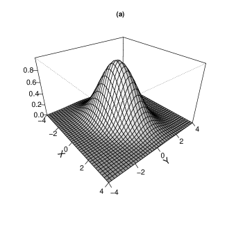
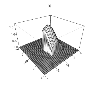
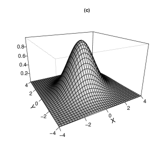
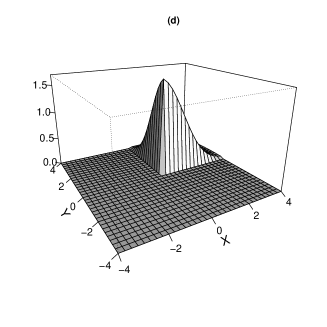
Figure 5.1: (a): The PDF of bivariate Gaussian distribution with parameters $\mu_{1}=\mu_{2}=0$, $\sigma_{1}^{2}=1$, $\sigma_{2}^{2}=2$, and $\rho=0.3535$. (b): The PDF of the corresponding truncated bivariate Gaussian distribution on area with lower limits $\bm{a}=(-1,-1)^{\top}$ and upper limits $\bm{b}=(2,2)^{\top}$. (c) The PDF of bivariate Gaussian distribution with parameters $\mu_{1}=\mu_{2}=0$, $\sigma_{1}^{2}=2$, $\sigma_{2}^{2}=2$, and $\rho=0.25$. (b): The PDF of the corresponding truncated bivariate Gaussian distribution on area with lower limits $\bm{a}=(0,0)^{\top}$ and upper limits $\bm{b}=(+\infty,+\infty)^{\top}$.

The corresponding R function for computing $\bm{\Omega}$ is given by the following.

⬇

1R> library(mvtnorm) # for computing multivariate Gaussian CDF

2R> a <- c(-1, -1); b <- c(2, 2); Mu <- c(0, 0);

3R> Sigma <- matrix( c(2, 0.5, 0.5, 2), nrow = length(Mu), ncol = length(Mu), byrow = TRUE)

4R> EX <- function(Mu, Sigma, a, b)

5+{

6+ if( any(a > b) == TRUE ) stop(message("lower␣bound␣must␣be␣smaller␣than␣the␣upper␣bound."))

7+ if( length(a) != length(Mu) || length(b) != length(Mu) ) stop(message("truncation␣bounds␣and␣location␣parameter␣must␣be␣of␣the␣same␣size."))

8+ p <- length(Mu)

9+ Omega <- numeric(p)

10+ V <- numeric(p)

11+ if(p == 2)

12+ {

13+ for(i in 1:p)

14+ {

15+ Mu_ia <- Sigma[i, -i]*(a[i] - Mu[i])/Sigma[i, i]

16+ Mu_ib <- Sigma[i, -i]*(b[i] - Mu[i])/Sigma[i, i]

17+ Delta_i <- sqrt( Sigma[-i, -i] - Sigma[i, -i]^2/Sigma[i, i] )

18+ V[i] <- dnorm(a[i] - Mu[i], 0, sd = sqrt(Sigma[i, i]) )*(

19+ pnorm(b[-i] - Mu[-i], mean = Mu_ia, sd = Delta_i)-

20+ pnorm(a[-i] - Mu[-i], mean = Mu_ia, sd = Delta_i) )-

21+ dnorm(b[i] - Mu[i], 0, sd = sqrt(Sigma[i, i]) )*(

22+ pnorm(b[-i] - Mu[-i], mean = Mu_ib, sd = Delta_i)-

23+ pnorm(a[-i] - Mu[-i], mean = Mu_ib, sd = Delta_i) )

24+ }

25+ }else{

26+ for(i in 1:p)

27+ {

28+ Mu_ia <- Sigma[i, -i]*(a[i] - Mu[i])/Sigma[i, i]

29+ Mu_ib <- Sigma[i, -i]*(b[i] - Mu[i])/Sigma[i, i]

30+ Delta_i <- Sigma[-i, -i] - c(Sigma[i, -i]%*%t(Sigma[i, -i])/(Sigma[i, i]))

31+ V[i] <- dnorm(a[i] - Mu[i], 0, sqrt(Sigma[i, i]) )*

32+ pmvnorm(a[-i] - Mu[-i], b[-i] - Mu[-i], mean = Mu_ia, sigma = Delta_i)[1] -

33+ dnorm(b[i] - Mu[i], 0, sqrt(Sigma[i, i]) )*

34+ pmvnorm(a[-i] - Mu[-i], b[-i] - Mu[-i], mean = Mu_ib, sigma = Delta_i)[1]

35+ }

36+ }

37+ Omega <- Sigma%*%V/pmvnorm(a, b, mean = Mu, sigma = Sigma)[1] + Mu

38+ return(Omega)

39+ }

40R> EX(a, b, Mu, Sigma)

5.3 Second moment of truncated Gaussian distribution

Let $\bm{v}=\bigl{(}v_{1}\cdots,v_{p}\bigr{)}^{\top}$ represent a vector of $p$ real-valued constants. Based on vector $\bm{v}$, for $i<j$, we define the following notations.

$$\bm{v}_{i,j}[x,y]=\bigl{(}{v}_{1},\cdots,{v}_{i-1},x,{v}_{i+1},\cdots,{v}_{j-1},y,{v}_{j+1},\cdots,{v}_{p}\bigr{)},$$ (5.26)

$$\bm{v}[-i,-j]=\bigl{(}{v}_{1},\cdots,{v}_{i-1},{v}_{i+1},\cdots,{v}_{j-1},{v}_{j+1},\cdots,{v}_{p}\bigr{)},$$ (5.27)

$$\bm{v}[i,j]=\bigl{(}{v}_{i},{v}_{j}\bigr{)}.$$ (5.28)

Let $\bm{X}\sim{\cal{TN}}_{p}(\bm{\mu},\Sigma,\bm{a},\bm{b})$. By definition, the second (raw) moment of truncated Gaussian distribution is given by 5.3

$$\bm{\Omega}^{2}=E\bigl{(}\bm{X}\bm{X}^{\top}\bigr{)}= \frac{1}{{\bf{C}}_{G}{\cal{P}}_{G}}\int_{\bm{a}}^{\bm{b}}\bm{x}\bm{x}^{\top}\exp\Bigl{\{}-\frac{\delta(\bm{x}-\bm{\mu},\Sigma)}{2}\Bigr{\}}d\bm{x}.$$

We recall that ${\bf{C}}_{G}=(2\pi)^{p/2}|\Sigma|^{1/2}$, ${\cal{P}}_{G}=\bm{\Phi}_{p}\bigl{(}\bm{b}\big{|}\bm{\mu},{\Sigma}\bigr{)}-\bm{\Phi}_{p}\bigl{(}\bm{a}\big{|}\bm{\mu},{\Sigma}\bigr{)}$. Using matrix algebra, one can see that

$$\frac{\partial^{2}}{\partial\bm{\mu}\partial\bm{\mu}^{\top}}\exp\Bigl{\{}-\frac{\delta(\bm{x}-\bm{\mu},\Sigma)}{2}\Bigr{\}}= \Bigl{[}{\Sigma}^{-1}(\bm{x}-\bm{\mu})(\bm{x}-\bm{\mu})^{\top}\Sigma^{-1}-\Sigma^{-1}\Bigr{]}$$

$$\times\exp\Bigl{\{}-\frac{\delta(\bm{x}-\bm{\mu},\Sigma)}{2}\Bigr{\}}.$$ (5.29)

Integrating both sides of (5.3), then multiplying from left and right by $\Sigma$, and finally rearranging, we have

$$\bm{\Omega}^{2}= \bm{\Omega}\bm{\mu}^{\top}+\bm{\mu}\bm{\Omega}^{\top}-\bm{\mu}\bm{\mu}^{\top}+\Sigma+\frac{\Sigma}{{\bf{C}}_{G}{\cal{P}}_{G}}\int_{\bm{a}}^{\bm{b}}\frac{\partial^{2}}{\partial\bm{\mu}\partial\bm{\mu}^{\top}}\exp\Bigl{\{}-\frac{\delta(\bm{x}-\bm{\mu},\Sigma)}{2}\Bigr{\}}d\bm{x}\Sigma$$

$$= \bm{\Omega}\bm{\mu}^{\top}+\bm{\mu}\bm{\Omega}^{\top}-\bm{\mu}\bm{\mu}^{\top}+\Sigma+\frac{\Sigma}{{\bf{C}}_{G}{\cal{P}}_{G}}\frac{\partial^{2}}{\partial\bm{\mu}\partial\bm{\mu}^{\top}}\int_{\bm{a}-\bm{\mu}}^{\bm{b}-\bm{\mu}}\exp\Bigl{\{}-\frac{\delta(\bm{u},\Sigma)}{2}\Bigr{\}}d\bm{u}\Sigma$$

$$= \bm{\Omega}\bm{\mu}^{\top}+\bm{\mu}\bm{\Omega}^{\top}-\bm{\mu}\bm{\mu}^{\top}+\Sigma+\Sigma\bm{I}\Sigma,$$ (5.30)

where

$$\bm{I}=\frac{1}{{\bf{C}}_{G}{\cal{P}}_{G}}\frac{\partial^{2}}{\partial\bm{\mu}\partial\bm{\mu}^{\top}}\int_{\bm{a}-\bm{\mu}}^{\bm{b}-\bm{\mu}}\exp\Bigl{\{}-\frac{\delta(\bm{u},\Sigma)}{2}\Bigr{\}}d\bm{u}.$$ (5.31)

As it may seen, $\bm{I}$ is a $p\times p$ square matrix whose $(i,j)$th element is shown by $I_{i,j}$. In order to compute $I_{i,j}$, we consider three scenarios given by the following.

• Scenario 1: $i\neq j=1,\cdots,p$ and $p=2$

• Scenario 2: $i\neq j=1,\cdots,p$ and $p>2$

• Scenario 3: $i=j=1,\cdots,p$

In what follows, we proceed to compute $I_{i,j}$ under three scenarios mentioned above.

• Scenario 1 ($i\neq j=1,\cdots,p$, and $p=2$): It follows from (5.31) that

  $$I_{1,2}=\frac{1}{{\bf{C}}_{G}{\cal{P}}_{G}}\frac{\partial^{2}}{\partial\mu_{1}\partial\mu_{2}}\int_{a_{1}-\mu_{1}}^{b_{1}-\mu_{1}}\int_{a_{2}-\mu_{2}}^{b_{2}-\mu_{2}}\exp\Bigl{\{}-\frac{\delta(\bm{u},\Sigma)}{2}\Bigr{\}}du_{1}du_{2}.$$ (5.32)

  Applying the Leibniz integral rule for the RHS of (5.32), we have

  $$I_{1,2}=\frac{1}{{\cal{P}}_{G}}\Bigl{[}\phi\bigl{(}\bm{b}\big{|}\bm{\mu},\Sigma\bigr{)}-\phi\bigl{(}(b_{1},a_{2})\big{|}\bm{\mu},\Sigma\bigr{)}+\phi\bigl{(}\bm{a}\big{|}\bm{\mu},\Sigma\bigr{)}-\phi\bigl{(}(a_{1},b_{2})\big{|}\bm{\mu},\Sigma\bigr{)}\Bigr{]}.$$

  Obviously $I_{2,1}=I_{1,2}$.

• Scenario 2 ($i\neq j=1,\cdots,p$, and $p>2$): For a given vector $(x,y)^{\top}$, it can be seen that the quadratic form $\delta\bigl{(}\bm{u}_{i,j}[x,y],\Sigma\bigr{)}$, for which $\bm{u}_{i,j}[x,y]$ is defined in (5.26), can be decomposed as

  $$\delta\bigl{(}\bm{u}_{i,j}[x,y],\Sigma\bigr{)}=\delta_{ij}(x,y)+\delta\Bigl{(}\bm{u}[-i,-j]-\bm{\xi}(x,y),\Delta_{ij}\Bigr{)},$$ (5.33)

  where $\delta_{ij}(x,y)=(x,y)^{\top}\Sigma^{-1}_{{\cal{I}},{\cal{I}}}(x,y)$ for ${\cal{I}}=\{i,j\}$ and

  $$\bm{\xi}(x,y)= \Sigma_{-{\cal{I}},{\cal{I}}}\bigl{(}\Sigma_{{\cal{I}},{\cal{I}}}\bigr{)}^{-1}(x,y),$$ (5.34)

  $$\Delta_{ij}= \Sigma_{-{\cal{I}},-{\cal{I}}}-\Sigma_{-{\cal{I}},{\cal{I}}}\bigl{(}\Sigma_{{\cal{I}},{\cal{I}}}\bigr{)}^{-1}\Sigma_{{\cal{I}},-{\cal{I}}}.$$ (5.35)

  Herein, $\bm{\xi}(x,y)$ is a vector of length $p-2$, $\Delta_{ij}$ is a $(p-2)\times(p-2)$ positive definite scale matrix, and $2\times 2$ positive definite scale matrix matrix $\Sigma_{{\cal{I}},{\cal{I}}}$ is given by

  $$\Sigma_{{\cal{I}},{\cal{I}}}=\biggl{[}\begin{matrix}\Sigma_{i,i}&\Sigma_{i,j}\\ \Sigma_{j,i}&\Sigma_{j,j}\end{matrix}\biggr{]}.$$

  For constructing $(p-2)\times 2$ matrix $\Sigma_{-{\cal{I}},{\cal{I}}}$, first construct a two-column matrix based on the $i$th and $j$th columns of matrix $\Sigma$ and then remove $i$th and $j$th rows of the constructed two-column matrix. We apply the Leibniz integral rule twice to the RHS of (5.31), and simultaneously utilize the property (5.33), to see that

  $$I_{i,j}= \frac{1}{{\bf{C}}_{G}{\cal{P}}_{G}}\exp\Bigl{\{}-\frac{\delta_{ij}(\bm{b}[i,j]-\bm{\mu}[i,j])}{2}\Bigr{\}}\times I_{1}\bigl{(}\bm{b}[i,j]\bigr{)}$$

  $$-\frac{1}{{\bf{C}}_{G}{\cal{P}}_{G}}\exp\Bigl{\{}-\frac{\delta_{ij}\bigl{(}(\bm{a}[i],\bm{b}[j])-\bm{\mu}[i,j]\bigr{)}}{2}\Bigr{\}}\times I_{1}\bigl{(}\bm{a}[i],\bm{b}[j]\bigr{)}$$

  $$-\frac{1}{{\bf{C}}_{G}{\cal{P}}_{G}}\exp\Bigl{\{}-\frac{\delta_{ij}\bigl{(}(\bm{b}[i],\bm{a}[j])-\bm{\mu}[i,j]\bigr{)}}{2}\Bigr{\}}\times I_{1}\bigl{(}\bm{b}[i],\bm{a}[j]\bigr{)}$$

  $$+\frac{1}{{\bf{C}}_{G}{\cal{P}}_{G}}\exp\Bigl{\{}-\frac{\delta_{ij}(\bm{a}[i,j]-\bm{\mu}[i,j])}{2}\Bigr{\}}\times I_{1}\bigl{(}\bm{a}[i,j]\bigr{)},$$ (5.36)

  where

  $$I_{1}(\bm{z})= \int_{\bm{a}[-i,-j]-\bm{\mu}[-i,-j]}^{\bm{b}[-i,-j]-\bm{\mu}[-i,-j]}\exp\Bigl{\{}-\frac{1}{2}\delta\Bigl{(}\bm{u}[-i,-j]-\bm{\xi}(\bm{z}),\Delta_{ij}\Bigr{)}\Bigr{\}}d\bm{u}[-i,-j].$$ (5.37)

  We further notice that the quantity ${\bf{C}}_{G}$ can be represented as

  $${\bf{C}}_{G}=(2\pi)^{\frac{p}{2}}|\Sigma|^{\frac{1}{2}}={2\pi\big{|}\Sigma_{{\cal{I}},{\cal{I}}}\big{|}^{\frac{1}{2}}}(2\pi)^{\frac{p-2}{2}}\big{|}\Delta_{ij}\big{|}^{\frac{1}{2}}.$$ (5.38)

  Substituting (5.38) into the RHS of (• ‣ 5.3), it follows that

  $$I_{i,j}= \frac{1}{{\cal{P}}_{G}}\bm{\phi}_{2}\Bigl{(}\bm{b}[i,j]\Big{|}\bm{\mu}[i,j],\Sigma_{{\cal{I}},{\cal{I}}}\Bigr{)}\times I_{2}(\bm{b}[i,j])$$

  $$-\frac{1}{{\cal{P}}_{G}}\bm{\phi}_{2}\Bigl{(}(\bm{a}[i],\bm{b}[j])\Big{|}\bm{\mu}[i,j],\Sigma_{{\cal{I}},{\cal{I}}}\Bigr{)}\times I_{2}(\bm{a}[i],\bm{b}[j])$$

  $$-\frac{1}{{\cal{P}}_{G}}\bm{\phi}_{2}\Bigl{(}(\bm{b}[i],\bm{a}[j])\Big{|}\bm{\mu}[i,j],\Sigma_{{\cal{I}},{\cal{I}}}\Bigr{)}\times I_{2}(\bm{b}[i],\bm{a}[j])$$

  $$+\frac{1}{{\cal{P}}_{G}}\bm{\phi}_{2}\Bigl{(}\bm{b}[i,j]\Big{|}\bm{\mu}[i,j],\Sigma_{{\cal{I}},{\cal{I}}}\Bigr{)}\times I_{2}(\bm{a}[i,j]),$$ (5.39)

  where

  $$I_{2}(\bm{z})= \bm{\Phi}_{p-2}\Bigl{(}\bm{b}[-i,-j]-\bm{\mu}[-i,-j]\Big{|}\bm{\xi}(\bm{z}),\Delta_{ij}\Bigr{)}$$

  $$-\bm{\Phi}_{p-2}\Bigl{(}\bm{b}[-i,-j]-\bm{\mu}[-i,-j]\Big{|}\bm{\xi}(\bm{z}),\Delta_{ij}\Bigr{)}.$$

  The matrix $\bm{I}$ is constructed by computing $I_{i,j}$ in (• ‣ 5.3) for all $i\neq j=1,\cdots,p$. The second moment of truncated Gaussian distribution is then obtained by substituting $\bm{I}$ into the RHS of (5.3).

• Scenario 3 ($i=j=1,\cdots,p$): Using the Leibniz integral rule, the first order derivative of the RHS of (5.31) is

  $$\frac{\partial}{\partial{\mu}_{i}}\bm{I}= \frac{1}{{\bf{C}}_{G}{\cal{P}}_{G}}\frac{\partial}{\partial{\mu}_{i}}\int_{\bm{a}-\bm{\mu}}^{\bm{b}-\bm{\mu}}\exp\Bigl{\{}-\frac{\delta(\bm{u},\Sigma)}{2}\Bigr{\}}d\bm{u}$$

  $$= \frac{1}{{\bf{C}}_{G}{\cal{P}}_{G}}\int_{\bm{a}[-i]-\bm{\mu}[-i]}^{\bm{b}[-i]-\bm{\mu}[-i]}\biggl{[}\exp\Bigl{\{}-\frac{\delta\bigl{(}\bm{u}_{i}[a_{i}-\mu_{i}],\Sigma\bigr{)}}{2}\Bigr{\}}$$

  $$-\exp\Bigl{\{}-\frac{\delta\bigl{(}\bm{u}_{i}[b_{i}-\mu_{i}],\Sigma\bigr{)}}{2}\Bigr{\}}\biggr{]}d\bm{u}[-i],$$ (5.40)

  for $i=1,\cdots,p$. We note that the quadratic form $\delta\bigl{(}\bm{u}_{i}[x],\Sigma\bigr{)}$, for which $\bm{u}_{i}[x]$ is defined in (5.26), can be decomposed as

  $$\delta\bigl{(}\bm{u}_{i}[x],\Sigma\bigr{)}=\delta_{ii}(x,x)+\delta\Bigl{(}\bm{u}[-i]-\bm{\xi}(x),\Delta_{ii}\Bigr{)},$$ (5.41)

  where $\delta_{ii}(x,x)=\bigl{(}x_{i}-\mu_{i}\bigr{)}^{2}\times\bigl{(}\Sigma_{i,i}\bigr{)}^{-1}$ is a scalar and

  $$\bm{\xi}(x)= \Sigma_{i,-i}\times\bigl{(}\Sigma_{i,i}\bigr{)}^{-1}\times x,$$ (5.42)

  $$\Delta_{ii}= \Sigma_{-i,-i}-\Sigma_{i,-i}\bigl{(}\Sigma_{i,-i}\bigr{)}^{\top}\times\bigl{(}\Sigma_{i,i}\bigr{)}^{-1}.$$ (5.43)

  We note that $\bm{\xi}(x)$ is a vector of length $p-1$ and $\Delta_{ii}$ is a $(p-1)\times(p-1)$ positive definite scale matrix. We further notice that the quantity ${\bf{C}}_{G}$ can be represented as

  $${\bf{C}}_{G}={(2\pi)^{\frac{1}{2}}\big{|}\Sigma_{i,i}\big{|}^{\frac{1}{2}}}(2\pi)^{\frac{p-1}{2}}\big{|}\Delta_{i}\big{|}^{\frac{1}{2}}.$$ (5.44)

  Using information given in (5.41), (5.42), (5.43), and (5.44), the RHS of (• ‣ 5.3) can be represented as

  $$\frac{\partial}{\partial{\mu}_{i}}\bm{I}= \frac{1}{{\cal{P}}_{G}}{\phi}\Bigl{(}a_{i}\Big{|}{\mu}_{i},\Sigma_{i,i}\Bigr{)}\times\biggl{[}\bm{\Phi}_{p-1}\Bigl{(}\bm{b}[-i]-\bm{\mu}[-i]\Big{|}\bm{\xi}({a}_{i}-{\mu}_{i}),\Delta_{ii}\Bigr{)}$$

  $$-\bm{\Phi}_{p-1}\Bigl{(}\bm{a}[-i]-\bm{\mu}[-i]\Big{|}\bm{\xi}({a}_{i}-{\mu}_{i}),\Delta_{ii}\Bigr{)}\biggr{]}-$$

  $$\frac{1}{{\cal{P}}_{G}}{\phi}\Bigl{(}{b}_{i}\Big{|}{\mu}_{i},\Sigma_{i,i}\Bigr{)}\times\biggl{[}\bm{\Phi}_{p-1}\Bigl{(}\bm{b}[-i]-\bm{\mu}_{i}\Big{|}\bm{\xi}({b}_{i}-{\mu}_{i}),\Delta_{ii}\Bigr{)}$$

  $$-\bm{\Phi}_{p-1}\Bigl{(}\bm{a}[-i]-\bm{\mu}[-i]\Big{|}\bm{\xi}({b}_{i}-{\mu}_{i}),\Delta_{ii}\Bigr{)}\biggr{]}$$

  $$= {I}_{ia}-{I}_{ib}.$$ (5.45)

  Now, taking the second partial derivative with respect to $\mu_{i}$ from RHS of (• ‣ 5.3), we obtain

  $$\frac{\partial{I}_{ia}}{\partial{\mu}_{i}}= \frac{\bigl{(}a_{i}-{\mu}_{i}\bigr{)}}{\Sigma_{i,i}\times{\cal{P}}_{G}}{\phi}\Bigl{(}a_{i}\Big{|}{\mu}_{i},\Sigma_{i,i}\Bigr{)}\biggl{[}\bm{\Phi}_{p-1}\Bigl{(}\bm{b}[-i]-\bm{\mu}[-i]\Big{|}\bm{\xi}({a}_{i}-{\mu}_{i}),\Delta_{ii}\Bigr{)}-$$

  $$\bm{\Phi}_{p-1}\Bigl{(}\bm{a}[-i]-\bm{\mu}[-i]\Big{|}\bm{\xi}({a}_{i}-{\mu}_{i}),\Delta_{ii}\Bigr{)}\biggr{]}-\frac{{\phi}\bigl{(}a_{i}\big{|}{\mu}_{i},\Sigma_{i,i}\bigr{)}}{\Sigma_{i,i}\times{\cal{P}}_{G}}\times\Sigma_{-i,i}\bigl{(}\Delta_{ii}\bigr{)}^{-1}\times$$

  $$\int_{\bm{a}[-i]-\bm{\mu}[-i]}^{\bm{b}[-i]-\bm{\mu}[-i]}\Bigl{(}\bm{u}[-i]-\bm{\xi}({a}_{i}-{\mu}_{i})\Bigr{)}\exp\Bigl{\{}-\frac{\delta\bigl{(}\bm{u}[-i]-\bm{\xi}({a}_{i}-{\mu}_{i}),\Delta_{ii}\bigr{)}}{2}\Bigr{\}}d\bm{u}[-i].$$ (5.46)

  Clearly, the RHS of (• ‣ 5.3) can be represented in terms of the first moment of a truncated Gaussian distribution. That means

  $$\frac{\partial{I}_{ia}}{\partial{\mu}_{i}}= \frac{1}{\Sigma_{i,i}\times{\cal{P}}_{G}}{\phi}\Bigl{(}a_{i}\Big{|}{\mu}_{i},\Sigma_{i,i}\Bigr{)}\biggl{[}\bm{\Phi}_{p-1}\Bigl{(}\bm{b}[-i]-\bm{\mu}[-i]\Big{|}\bm{\xi}({a}_{i}-{\mu}_{i}),\Delta_{ii}\Bigr{)}-$$

  $$\bm{\Phi}_{p-1}\Bigl{(}\bm{a}[-i]-\bm{\mu}[-i]\Big{|}\bm{\xi}({a}_{i}-{\mu}_{i}),\Delta_{ii}\Bigr{)}\biggr{]}\times\Bigl{[}a_{i}-\mu_{i}-\Sigma_{-i,i}\bigl{(}\Delta_{ii}\bigr{)}^{-1}\bm{\Omega}_{a}\Bigr{]},$$ (5.47)

  where

  $$\bm{\Omega}_{a}=E\Bigl{(}\bm{Y}_{a}\Big{|}\bm{a}[-i]-\bm{\mu}[-i]-\bm{\xi}({a}_{i}-{\mu}_{i})<\bm{Y}_{a}<\bm{b}[-i]-\bm{\mu}[-i]-\bm{\xi}({a}_{i}-{\mu}_{i})\Bigr{)},$$

  in which $\bm{Y}_{a}\sim{\cal{N}}_{p-1}\bigl{(}\bm{0},\Delta_{ii}\bigr{)}$. For computing $\partial{I}_{ib}/\partial{\mu}_{i}$, we likewise have

  $$\frac{\partial{I}_{ib}}{\partial{\mu}_{i}}= \frac{1}{\Sigma_{i,i}\times{\cal{P}}_{G}}{\phi}\Bigl{(}b_{i}\Big{|}{\mu}_{i},\Sigma_{i,i}\Bigr{)}\biggl{[}\bm{\Phi}_{p-1}\Bigl{(}\bm{b}[-i]-\bm{\mu}[-i]\Big{|}\bm{\xi}({b}_{i}-{\mu}_{i}),\Delta_{ii}\Bigr{)}-$$

  $$\bm{\Phi}_{p-1}\Bigl{(}\bm{a}[-i]-\bm{\mu}[-i]\Big{|}\bm{\xi}({b}_{i}-{\mu}_{i}),\Delta_{ii}\Bigr{)}\biggr{]}\times\Bigl{[}b_{i}-\mu_{i}-\Sigma_{-i,i}\bigl{(}\Delta_{ii}\bigr{)}^{-1}\bm{\Omega}_{b}\Bigr{]},$$ (5.48)

  where

  $$\bm{\Omega}_{b}=E\Bigl{(}\bm{Y}_{b}\Big{|}\bm{a}[-i]-\bm{\mu}[-i]-\bm{\xi}({b}_{i}-{\mu}_{i})<\bm{Y}_{b}<\bm{b}[-i]-\bm{\mu}[-i]-\bm{\xi}({b}_{i}-{\mu}_{i})\Bigr{)},$$

  in which $\bm{Y}_{b}\sim{\cal{N}}_{p-1}\bigl{(}\bm{0},\Delta_{ii}\bigr{)}$. Once we have computed $\partial{I}_{ia}/\partial{\mu}_{i}$ in (• ‣ 5.3) and $\partial{I}_{ib}/\partial{\mu}_{i}$ in (• ‣ 5.3), for $i=1,\cdots,p$, then the diagonal elements of $\bm{I}$ given by (5.3) are available.

Once we have construct matrix $\bm{I}$, we can compute $\bm{\Omega}^{2}$ by substituting computed $\bm{I}$ at the RHS of (5.3).

Herein, we carry out a small simulation study for computing the first moment of vector $(X,Y)^{\top}$ under two scenarios. Within the first scenario, we assume that $(X,Y)^{\top}$ follows truncated bivariate Gaussian distribution with parameters $\bm{\mu}=\bm{0}$, $\Sigma\leavevmode\nobreak\ \bigl{(}\sigma_{1}^{2}=2,\sigma_{2}^{2}=1,\rho=0.3535\bigr{)}$ truncated on area with lower limits $\bm{a}=(-1,-1)^{\top}$ and upper limits $\bm{b}=(2,2)^{\top}$. Under the second scenario it is assumed that $(X,Y)^{\top}$ follows truncated bivariate Gaussian distribution with parameters $\bm{\mu}=\bm{0}$, $\Sigma$ $\bigl{(}\sigma_{1}^{2}=2,\sigma_{2}^{2}=2,\rho=0.25\bigr{)}$ truncated on area with lower limits $\bm{a}=(0,0)^{\top}$ and upper limits $\bm{b}=(+\infty,+\infty)^{\top}$. We note that the concern of the second scenario is placed on computing the absolute moment, that is $\bm{\Omega}=E(|\bm{X}|)$. For both scenario, we compute $\bm{\Omega}$ by generating samples of sizes $N=2000,5000$, and 20000 based on 5000 runs. The instrumental distribution is set to be ${\cal{N}}_{2}(\bm{\mu},\Sigma)$. For computing $\bm{\Omega}=E\bigl{(}\bm{{\cal{X}}}_{a,b}\bigr{)}$ through the ${\cal{N}}_{2}(\bm{\mu},\Sigma)$, one can follow two ways. In the first way the quantity $\bm{\Omega}$ is estimated as

$$\hat{\bm{\Omega}}=\frac{1}{N}\sum_{i=1}^{N}|\bm{x}_{i}\big{|}$$ (5.49)

where $\big{|}\bm{x}_{i}\big{|}=\bigl{(}\big{|}x_{1i}\big{|},\big{|}x_{2i}\big{|}\bigr{)}^{\top}$ where $\bm{x}_{i}$s come independently from ${\cal{N}}_{2}(\bm{\mu},\Sigma)$, for sufficiently large $N$. The second method proceeds to compute $\hat{\bm{\Omega}}$ based on sample of size $N$ when the lower and upper truncation bounds are $\bm{a}=\bm{0}$ and $\bm{b}=+\bm{\infty}$, respectively. Details for implementing the second method are given as follows. The corresponding R function EXX for computing $\bm{\Omega}$ is given by the following.

⬇

1R> library(mvtnorm) # for computing multivariate Gaussian CDF

2R> EXX <- function(Mu, Sigma, a, b)

3+{

4+ if(any(a>b) == TRUE) stop(message("vector␣a␣must␣be␣smaller␣than␣vector␣b."))

5+ p <- length(Mu)

6+ PG <- pmvnorm(lower = a, upper = b, mean = Mu, sigma = Sigma)[1]

7+ II <- matrix(0, nrow = p, ncol = p)

8+ if( p == 2 )

9+ {

10+ for(i in 1:p){

11+ Mu_ia <- Sigma[i, -i]*(a[i] - Mu[i])/Sigma[i, i]

12+ Mu_ib <- Sigma[i, -i]*(b[i] - Mu[i])/Sigma[i, i]

13+ Delta_i <- Sigma[-i, -i] - Sigma[i, -i]*Sigma[i, -i]/Sigma[i, i]

14+ La_i <- a[-i] - Mu[-i] - Mu_ia

15+ Ua_i <- b[-i] - Mu[-i] - Mu_ia

16+ Lb_i <- a[-i] - Mu[-i] - Mu_ib

17+ Ub_i <- b[-i] - Mu[-i] - Mu_ib

18+ PG_ia <- pnorm( Ua_i, mean = rep(0, p-1), sd = sqrt( Delta_i) )-

19+ pnorm( La_i, mean = rep(0, p-1), sd = sqrt( Delta_i) )

20+ PG_ib <- pnorm( Ub_i, mean = rep(0, p-1), sd = sqrt( Delta_i) )-

21+ pnorm( Lb_i, mean = rep(0, p-1), sd = sqrt( Delta_i) )

22+ Ex_ia <- Delta_i*( dnorm(La_i, 0, sqrt(Delta_i)) -

23+ dnorm(Ua_i, 0, sqrt(Delta_i)))/PG_ia

24+ Ex_ib <- Delta_i*( dnorm(Lb_i, 0, sqrt(Delta_i)) -

25+ dnorm(Ub_i, 0, sqrt(Delta_i)))/PG_ib

26+ p1 <-(a[i]-Mu[i])/(PG*Sigma[i, i])*dnorm(a[i]-Mu[i],0,sqrt(Sigma[i, i]) )*(

27+ pnorm(b[-i] - Mu[-i], mean = Mu_ia, sd = sqrt( Delta_i) )-

28+ pnorm(a[-i] - Mu[-i], mean = Mu_ia, sd = sqrt( Delta_i) ) )-

29+ PG_ia/PG*dnorm(a[i] - Mu[i], 0, sqrt(Sigma[i, i]) )*

30+ Sigma[i,-i]*Ex_ia/(Delta_i*Sigma[i, i])

31+ p2 <- -(b[i]-Mu[i])/(PG*Sigma[i, i])*dnorm(b[i]-Mu[i],0,sqrt(Sigma[i, i]))*(

32+ pnorm(b[-i] - Mu[-i], mean = Mu_ib, sd = sqrt( Delta_i) )-

33+ pnorm(a[-i] - Mu[-i], mean = Mu_ib, sd = sqrt( Delta_i) ) ) +

34+ PG_ib/PG*dnorm(b[i] - Mu[i], 0, sqrt(Sigma[i, i]) )*

35+ Sigma[i,-i]*Ex_ib/(Delta_i*Sigma[i, i])

36+ II[i, i] <- p1 + p2

37+ }

38+ x_aa <- a - Mu

39+ x_ab <- c(a[1] - Mu[1], b[2] - Mu[2])

40+ x_ba <- c(b[1] - Mu[1], a[2] - Mu[2])

41+ x_bb <- b - Mu

42+ II[1, 2] <-( dmvnorm(x_bb, mean = rep(0, p), sigma = Sigma )-

43+ dmvnorm(x_ab, mean = rep(0, p), sigma = Sigma )-

44+ dmvnorm(x_ba, mean = rep(0, p), sigma = Sigma )+

45+ dmvnorm(x_aa, mean = rep(0, p), sigma = Sigma ))/PG

46+ II[2, 1] <- II[1, 2]

47+ }

48+ if( p == 3 )

49+ {

50+ for(i in 1:(p - 1)){

51+ for(j in (i + 1):p){

52+ I_ij <- c(i, j)

53+ Sigma_ij <- Sigma[I_ij, I_ij]

54+ I0 <- Sigma[I_ij, -I_ij]%*%solve(Sigma_ij)

55+ x_aa <- c(a[i] - Mu[i], a[j] - Mu[j])

56+ x_ab <- c(a[i] - Mu[i], b[j] - Mu[j])

57+ x_ba <- c(b[i] - Mu[i], a[j] - Mu[j])

58+ x_bb <- c(b[i] - Mu[i], b[j] - Mu[j])

59+ Mu_aa <- (I0%*%x_aa)[1]

60+ Mu_ab <- (I0%*%x_ab)[1]

61+ Mu_ba <- (I0%*%x_ba)[1]

62+ Mu_bb <- (I0%*%x_bb)[1]

63+ Delta_ij <- Sigma[-I_ij, -I_ij] - ( I0%*%Sigma[-I_ij, I_ij] )[1]

64+ p1 <- dmvnorm(x_bb, mean = rep(0, 2), sigma = Sigma_ij)*(

65+ pnorm(b[-I_ij] - Mu[-I_ij], mean = Mu_bb, sd = sqrt( Delta_ij ) )-

66+ pnorm(a[-I_ij] - Mu[-I_ij], mean = Mu_bb, sd = sqrt( Delta_ij ) ) )

67+ p2 <- dmvnorm(x_ab, mean = rep(0, 2), sigma = Sigma_ij)*(

68+ pnorm(b[-I_ij] - Mu[-I_ij], mean = Mu_ab, sd = sqrt( Delta_ij ) )-

69+ pnorm(a[-I_ij] - Mu[-I_ij], mean = Mu_ab, sd = sqrt( Delta_ij ) ) )

70+ p3 <- dmvnorm(x_ba, mean = rep(0, 2), sigma = Sigma_ij)*(

71+ pnorm(b[-I_ij] - Mu[-I_ij], mean = Mu_ba, sd = sqrt( Delta_ij ) )-

72+ pnorm(a[-I_ij] - Mu[-I_ij], mean = Mu_ba, sd = sqrt( Delta_ij ) ) )

73+ p4 <- dmvnorm(x_aa, mean = rep(0, 2), sigma = Sigma_ij)*(

74+ pnorm(b[-I_ij] - Mu[-I_ij], mean = Mu_aa, sd = sqrt( Delta_ij ) )-

75+ pnorm(a[-I_ij] - Mu[-I_ij], mean = Mu_aa, sd = sqrt( Delta_ij ) ) )

76+ II[i, j] <- (p1 - p2 - p3 + p4)/PG

77+ II[j, i] <- II[i, j]

78+ }

79+ }

80+ for(i in 1:p){

81+ Mu_ia <- Sigma[i, -i]*(a[i] - Mu[i])/Sigma[i, i]

82+ Mu_ib <- Sigma[i, -i]*(b[i] - Mu[i])/Sigma[i, i]

83+ Delta_i <- Sigma[-i, -i] - Sigma[i, -i]%*%t(Sigma[i, -i])/Sigma[i, i]

84+ La_i <- a[-i] - Mu[-i] - Mu_ia

85+ Ua_i <- b[-i] - Mu[-i] - Mu_ia

86+ Lb_i <- a[-i] - Mu[-i] - Mu_ib

87+ Ub_i <- b[-i] - Mu[-i] - Mu_ib

88+ PG_ia <- pmvnorm(lower=La_i, upper=Ua_i, mean=rep(0, p-1), sigma=Delta_i)[1]

89+ PG_ib <- pmvnorm(lower=Lb_i, upper=Ub_i, mean=rep(0, p-1), sigma=Delta_i)[1]

90+ p5 <- (a[i]-Mu[i])/(PG*Sigma[i, i])*dnorm(a[i]-Mu[i],0,sqrt(Sigma[i, i]) )*

91+ pmvnorm(a[-i] - Mu[-i], b[-i] - Mu[-i], mean = Mu_ia, sigma = Delta_i)[1] -

92+ PG_ia/PG*dnorm(a[i]-Mu[i],0,sqrt(Sigma[i, i]) )*(t(Sigma[i, -i])%*%

93+ solve(Delta_i)%*%EX( rep(0,p-1), Delta_i, La_i, Ua_i)/Sigma[i, i])[1]

94+ p6 <- -(b[i]-Mu[i])/(PG*Sigma[i, i])*dnorm(b[i]-Mu[i],0,sqrt(Sigma[i, i]) )*

95+ pmvnorm(a[-i] - Mu[-i], b[-i] - Mu[-i], mean = Mu_ib, sigma = Delta_i)[1] +

96+ PG_ib/PG*dnorm(b[i] - Mu[i],0, sqrt(Sigma[i, i]) )*(t(Sigma[i, -i])%*%

97+ solve(Delta_i)%*%EX(rep(0,p-1), Delta_i, Lb_i, Ub_i)/Sigma[i, i])[1]

98+ II[i, i] <- p5 + p6

99+ }

100+ }

101+ if ( p > 3 )

102+ {

103+ for(i in 1:(p - 1)){

104+ for(j in (i + 1):p){

105+ I_ij <- c(i, j)

106+ Sigma_ij <- Sigma[I_ij, I_ij]

107+ I0 <- Sigma[-I_ij, I_ij]%*%solve(Sigma_ij)

108+ x_aa <- c( a[i] - Mu[i], a[j] - Mu[j] )

109+ x_ab <- c( a[i] - Mu[i], b[j] - Mu[j] )

110+ x_ba <- c( b[i] - Mu[i], a[j] - Mu[j] )

111+ x_bb <- c( b[i] - Mu[i], b[j] - Mu[j] )

112+ Mu_aa <- c( I0%*%x_aa )

113+ Mu_ab <- c( I0%*%x_ab )

114+ Mu_ba <- c( I0%*%x_ba )

115+ Mu_bb <- c( I0%*%x_bb )

116+ Delta_ij <- Sigma[-I_ij, -I_ij] - ( I0%*%Sigma[-I_ij, I_ij] )[1]

117+ p1 <- dmvnorm(x_bb, mean = rep(0, 2), sigma = Sigma_ij)*

118+ pmvnorm(a[-I_ij]-Mu[-I_ij], b[-I_ij]-Mu[-I_ij], mean = Mu_bb, sigma=Delta_ij )

119+ p2 <- dmvnorm(x_ab, mean = rep(0, 2), sigma = Sigma_ij)*

120+ pmvnorm(a[-I_ij]-Mu[-I_ij], b[-I_ij]-Mu[-I_ij], mean = Mu_ab, sigma=Delta_ij )

121+ p3 <- dmvnorm(x_ba, mean = rep(0, 2), sigma = Sigma_ij)*

122+ pmvnorm(a[-I_ij]-Mu[-I_ij], b[-I_ij]-Mu[-I_ij], mean = Mu_ba, sigma=Delta_ij )

123+ p4 <- dmvnorm(x_aa, mean = rep(0, 2), sigma = Sigma_ij)*

124+ pmvnorm(a[-I_ij]-Mu[-I_ij], b[-I_ij]-Mu[-I_ij], mean = Mu_aa, sigma=Delta_ij )

125+ II[i, j] <- (p1 - p2 - p3 + p4)/PG

126+ II[j, i] <- II[i, j]

127+ }

128+ }

129+ for(i in 1:p){

130+ Mu_ia <- Sigma[i, -i]*(a[i] - Mu[i])/Sigma[i, i]

131+ Mu_ib <- Sigma[i, -i]*(b[i] - Mu[i])/Sigma[i, i]

132+ Delta_i <- Sigma[-i, -i] - Sigma[i, -i]%*%t(Sigma[i, -i])/Sigma[i, i]

133+ La_i <- a[-i] - Mu[-i] - Mu_ia

134+ Ua_i <- b[-i] - Mu[-i] - Mu_ia

135+ Lb_i <- a[-i] - Mu[-i] - Mu_ib

136+ Ub_i <- b[-i] - Mu[-i] - Mu_ib

137+ PG_ia <- pmvnorm(lower=La_i, upper=Ua_i, mean=rep(0, p-1), sigma=Delta_i)[1]

138+ PG_ib <- pmvnorm(lower=Lb_i, upper=Ub_i, mean=rep(0, p-1), sigma=Delta_i)[1]

139+ p5 <- (a[i]-Mu[i])/(PG*Sigma[i, i])*dnorm(a[i] - Mu[i], 0, sqrt(Sigma[i, i]))*

140+ pmvnorm(a[-i] - Mu[-i], b[-i] - Mu[-i], mean=Mu_ia, sigma=Delta_i)[1] -

141+ PG_ia/PG*dnorm(a[i] - Mu[i], 0, sqrt(Sigma[i, i]) )*(t(Sigma[i, -i])%*%

142+ solve(Delta_i)%*%EX( rep(0, p - 1), Delta_i, La_i, Ua_i)/Sigma[i, i])[1]

143+ p6 <- -(b[i]-Mu[i])/(PG*Sigma[i, i])*dnorm(b[i]-Mu[i],0,sqrt(Sigma[i, i]) )*

144+ pmvnorm(a[-i] - Mu[-i], b[-i] - Mu[-i], mean = Mu_ib, sigma = Delta_i)[1] +

145+ PG_ib/PG*dnorm(b[i] - Mu[i], 0, sqrt(Sigma[i, i]))*(t(Sigma[i, -i])%*%

146+ solve(Delta_i)%*%EX(rep(0, p - 1), Delta_i, Lb_i, Ub_i)/Sigma[i, i])[1]

147+ II[i, i] <- p5 + p6

148+ }

149+ }

150+ Omega <- EX(Mu, Sigma, a, b)

151+ EXX <- Omega%*%Mu + t(Omega%*%Mu) - Mu%*%t(Mu) + Sigma + Sigma%*%II%*%Sigma

152+ return(EXX)

153+ }

5.4 Truncated skew Gaussian distribution

Here, we introduce the class of skew Gaussian distributions that is known in the literature as the canonical fundamental unrestricted skew Gaussian distribution, see Arellano-Valle and Azzalini (2006). We write $\bm{X}\sim\text{SG}_{p,q}(\bm{\mu},\Sigma,{\Lambda})$ to denote that $p$-dimensional random vector $\bm{X}$ follows a canonical fundamental unrestricted skew Gaussian distribution with PDF given by

$$f(\bm{x}\big{|}\bm{\mu},{\Sigma},{{\Lambda}})=2^{q}\bm{\phi}_{p}\bigl{(}\bm{x}|\bm{\mu},{\Omega}\bigr{)}\bm{\Phi}_{q}\bigl{(}\bm{m}|\bm{0}_{q},{\Delta}\bigr{)},$$ (5.50)

where ${\Omega}={\Sigma}+{{\Lambda}}{{\Lambda}}^{\top}$, ${\Delta}=\bm{I}_{q}-{{\Lambda}}^{\top}{\Omega}^{-1}{{\Lambda}}$, $\bm{m}={\Lambda}^{\top}{{\Omega}}^{-1}(\bm{y}-\bm{\mu})$, and $\bm{I}_{q}$ denotes the $q\times q$ identity matrix. Further, $\bm{\phi}_{p}\bigl{(}.\big{|}\bm{\mu},{\Omega}\bigr{)}$ denotes the PDF of a $p$-dimensional Gaussian distribution with location vector $\bm{\mu}$ and dispersion matrix $\Sigma$, and $\bm{\Phi}_{q}\bigl{(}.\big{|}\bm{0}_{q},{\Delta}\bigr{)}$ is the CDF of a $q$-dimensional Gaussian distribution with location vector $\bm{0}_{q}$ (a vector of zeros of length $q$) and dispersion matrix ${\Delta}$. The random vector $\bm{X}$ admits stochastic representation as follows, see (Arellano-Valle and Genton, 2005; Arellano-Valle and Azzalini, 2006; Arellano-Valle et al., 2007).

$$\bm{X}\mathop{=}\limits^{d}\bm{\mu}+{\Lambda}\big{|}\bm{Z}_{0}\big{|}+{\Sigma}^{\frac{1}{2}}\bm{Z}_{1},$$ (5.51)

where $\mathop{=}\limits^{d}$ means “distributed as” and random vectors $\bm{Z}_{0}\sim{\cal{N}}_{q}\bigl{(}\bm{0},\bm{I}_{q}\bigr{)}$ and $\bm{Z}_{1}\sim{\cal{N}}_{q}\bigl{(}\bm{0},\bm{I}_{p}\bigr{)}$ are independent. Furthermore, it can be seen that (Lee and McLachlan, 2016; Maleki et al., 2019; Morales et al., 2022)

$$\bm{X}\mathop{=}\limits^{d}\bm{\mu}+\bigl{(}\bm{W}\big{|}\bm{W}_{0}>\bm{0}\bigr{)},$$ (5.52)

in which

$$\bm{Y}=\biggl{[}\begin{matrix}\bm{W}_{0}\\ \bm{W}_{1}\end{matrix}\biggr{]}\sim{\cal{N}}_{q+p}\biggl{(}\biggl{[}\begin{matrix}\bm{0}_{q}\\ \bm{0}_{p}\end{matrix}\biggr{]},\biggl{[}\begin{matrix}\bm{I}_{q}&\bm{\Lambda}^{\top}\\ \bm{\Lambda}&{\Sigma}+\bm{\Lambda}\bm{\Lambda}^{\top}\\ \end{matrix}\biggr{]}\biggr{)}.$$ (5.53)

By the property (6.26), we can construct a method for simulating from $\bm{X}\big{|}\bm{a}<\bm{X}<\bm{b}$ when $\bm{X}$ admits relation (6.24). To this end, we need to simulate from $(p+q)$-dimensional Gaussian random vector $\bm{Y}$ given by (6.26). Some algebra show

$$\bm{X}\big{|}\bigl{(}\bm{a}<\bm{X}<\bm{b}\bigr{)}\mathop{=}\limits^{d}\bm{\mu}^{*}+\bm{Y}\big{|}\bigl{(}\bm{a}^{*}-\bm{\mu}^{*}<\bm{Y}<\bm{b}^{*}-\bm{\mu}^{*}\bigr{)},$$

where $a^{*}=\bigl{(}\bm{0}^{\top}_{q},\bm{a}^{\top}\bigr{)}^{\top}$, $b^{*}=\bigl{(}\bm{\infty}^{\top}_{q},\bm{b}^{\top}\bigr{)}^{\top}$, and $\bm{\mu}^{*}=\bigl{(}\bm{0}^{\top}_{q},\bm{\mu}^{\top}\bigr{)}^{\top}$ in which $\bm{\infty}_{q}$ is a vector of length $q$ of infinities. Hence, using the methodology given in Sections 5.2 and 5.3 for computing the first and second moments of multivariate Gaussian distribution, we can compute the first and second moments of truncated skew Gaussian distribution by computing $E\bigl{(}\bm{Y}\big{|}\bm{a}^{*}<\bm{Y}<\bm{b}^{*}\bigr{)}$ and $E\bigl{(}\bm{Y}\bm{Y}^{\top}\big{|}\bm{a}^{*}<\bm{Y}<\bm{b}^{*}\bigr{)}$, respectively. We note that an R package called MomTrunc uploaded at https://cran.r-project.org/web/packages/MomTrunc/inde
x.html developed for this aim (Morales et al., 2022). The following R code can be used for computing first two moments of the truncated random vector $\bm{X}$ where $\bm{X}\sim\text{SG}_{2,2}(\bm{\mu},\Sigma,{\Lambda})$ truncated on $(\bm{a},\bm{b})$ in which $\bm{\mu}=(0,0)^{\top}$, $\bm{a}=(-3,-3)^{\top}$, $\bm{b}=(2,2)^{\top}$,

$$\Sigma=\left[\begin{matrix}2&0.5\\ 0.5&2\\ \end{matrix}\right],\Lambda=\left[\begin{matrix}4&2\\ 2&-5\\ \end{matrix}\right].$$

⬇

1library("MomTrunc")

2a <- c(-3, -3); b <- c(2, 2); Mu <- c(0, 0); p <- 2; q<- 2

3a_star <- c(0, 0, a); b_star <- c(Inf, Inf, b); Mu_star <- c(0, 0, Mu)

4Sigma <- matrix( c(2, 0.5, 0.5, 2), nrow = p , ncol = p)

5ch <- t(chol(Sigma)); Lambda <- matrix( c(4, 2 ,2, -5 ), nrow = p , ncol = q)

6p1 <- diag(q); p2 <- t(Lambda); p3 <- t(p2); p4 <- Sigma + p3%*%t(p3)

7Sigma_star <- matrix(

8 c(p1[1,1],p1[1,2], p2[1,1], p2[1,2],

9 p1[2,1],p1[2,2], p2[2,1], p2[2,2],

10 p3[1,1],p3[1,2], p4[1,1], p4[1,2],

11 p3[2,1],p3[2,2], p4[2,1], p4[2,2]), nrow = p + q, ncol = p + q)

12out <- MCmeanvarTMD(a_star, b_star, rep(0, p + q), Sigma_star, dist = "normal")

13out$mean[(p+1):(p+q)]

14out$EYY[(p+1):(p+q), (p+1):(p+q)]

5.5 Gaussian scale mixture model

Here, we introduce the useful property known in the literature as Gaussian scale mixture model. Based on this property, one can represent the PDF and other characteristics of a wide range of distributions in terms of the Gaussian model.

Definition 5.5.1.

Let random variable $Z$ follows a standard Gaussian distribution. For given positive valued function $h(\cdot)$ and positive random variable $G$, the random variable $X$ is said to follow a Gaussian scale mixture model if we can write

$$X=\mu+\sigma\frac{Z}{h(G)},$$ (5.54)

where $\mu\in\mathbb{R}$ and $\sigma\in\mathbb{R}^{+}$ are the location and scale parameters, respectively. Herein, and random variable $G$ is the mixing variable.

Likewise, the multivariate version of the Gaussian scale mixture model (representation) is given as follows.

Definition 5.5.2.

Let random variable $\bm{Z}$ follows a $p$-dimensional standard Gaussian distribution. For given positive valued function $h(\cdot)$ and positive random variable $G$. The $p$-dimensional random vector $\bm{X}$ is said to follow a Gaussian scale mixture model if we have

$$\bm{X}=\bm{\mu}+A\frac{\bm{Z}}{h(G)}$$ (5.55)

where $\bm{\mu}\in\mathbb{R}^{p}$ and $p\times p$ lower triangular matrix $A$ is called the Cholesky decomposition of positive definite scale matrix $\Sigma$ such that $\Sigma=AA^{\top}$. Herein, the univariate random variable $G$ plays the role of the mixing variable.

The well-known example of Gaussian scale mixture model is the Student’s $t$ distribution, with PDF given by (5.56), for which $h(G)=\sqrt{G}$ where $G\sim{\cal{G}}(\nu/2,\nu/2)$.

5.6 Moment of truncated Student’s $t$ distribution

Let random vector $\bm{X}=(X_{1},\cdots,X_{p})^{\top}$ follows a $p$-dimensional Student’s $t$ distribution with $\nu>0$ degrees of freedom with PDF given by

$$f(\bm{x}\big{|}\bm{\Psi}\bigr{)}= \frac{\Gamma\bigl{(}\frac{\nu+p}{2}\bigr{)}}{(\nu\pi)^{\frac{p}{2}}\Gamma\bigl{(}\frac{\nu}{2}\bigr{)}|\Sigma|^{\frac{1}{2}}}\biggl{[}1+\frac{\delta(\bm{x}-\bm{\mu},\Sigma)}{\nu}\biggr{]}^{-\frac{\nu+p}{2}},$$ (5.56)

where $\bm{\Psi}=(\bm{\mu},\Sigma,\nu)$ is the parameter vector and Mahalanobis distance $\delta(\cdot)$ is defined in (6.3). By definition

$$E(\bm{X})= \int_{-\bm{\infty}}^{\bm{\infty}}\frac{\bm{x}\Gamma\bigl{(}\frac{\nu+p}{2}\bigr{)}}{(\nu\pi)^{\frac{p}{2}}\Gamma\bigl{(}\frac{\nu}{2}\bigr{)}|\Sigma|^{\frac{1}{2}}}\biggl{[}1+\frac{\delta(\bm{x}-\bm{\mu},\Sigma)}{\nu}\biggr{]}^{-\frac{\nu+p}{2}}d\bm{x},$$ (5.57)

for $\nu>1$. The first moment of the truncated Student’s $t$ distribution (shown by ${\cal{TT}}_{p}(\bm{\mu},\Sigma,\nu,\bm{a},\bm{b})$) can be evaluated through relation (5.6) in which $f(\bm{u})$ is replaced with $f(\bm{x}\big{|}\bm{\Psi}\bigr{)}$ given in (5.56) and $F(\bm{b})-F(\bm{a})=P(\bm{a}<\bm{X}<\bm{b})=\int_{\bm{a}}^{\bm{b}}f(\bm{x}\big{|}\bm{\Psi}\bigr{)}d\bm{x}$. However, herein, we proceed to compute $\bm{\Omega}=E\bigl{(}\bm{{{X}}}\big{|}\bm{a}<\bm{X}<\bm{b}\bigr{)}$ based on the property of Gaussian scale mixture model introduced in Section 5.5.

5.6.1 First two moments of truncated Student’s $t$ distribution distribution in univariate case

Herein, we proceed to compute the first and second moments of an univariate Student’s $t$ distribution. For simplicity, we use generic symbols ${t}\bigl{(}{x}\big{|}{\mu},\sigma^{2},\nu\bigr{)}$ and ${T}\bigl{(}{x}\big{|}{\mu},\sigma^{2},\nu\bigr{)}$ to denote, accordingly, the PDF and CDF of a Student’s $t$ distribution with $\nu$ degrees of freedom at point ${x}$ for which ${\mu}$, $\sigma$, and $\nu$ play the role of location, scale, and degrees of freedom parameters, respectively. Furthermore, we write ${X}\sim{t}({\mu},\sigma^{2},\nu)$ to show that random variable ${X}$ follows a Student’s $t$ distribution with location parameter ${\mu}$, scale parameter $\sigma$, and $\nu$ degrees of freedom. The corresponding truncated family on $(a,b)$ is represented by ${\cal{TT}}\bigl{(}{\mu},\sigma^{2},\nu,a,b\bigr{)}$.

If $X\sim t\bigl{(}\mu,\sigma^{2},\nu\bigr{)}$, it can be seen from (5.4) for $m=1$ that

$$\Omega= \frac{1}{{\cal{P}}_{t}}\int_{a}^{b}x\times{t}\bigl{(}{x}\big{|}{\mu},\sigma^{2},\nu\bigr{)}dx,$$

$$= \frac{1}{{\cal{P}}_{t}}\int_{a}^{b}\frac{x\Gamma\bigl{(}\frac{\nu+1}{2}\bigr{)}}{\sqrt{\nu\pi}\Gamma\bigl{(}\frac{\nu}{2}\bigr{)}\sigma|}\biggl{[}1+\frac{({x}-{\mu})^{2}}{\nu\sigma^{2}}\biggr{]}^{-\frac{\nu+1}{2}}d{x},$$ (5.58)

where ${\cal{P}}_{t}=T\bigl{(}{b}\big{|}{\mu},\sigma^{2},\nu\bigr{)}-{T}\bigl{(}{a}\big{|}{\mu},\sigma^{2},\nu\bigr{)}$. Rather computing $\Omega$ through (5.6.1), we prefer to use Definition 5.5.1 that states each Student’s $t$ distribution is a Gaussian scale mixture model. In fact ${X}$ admits the hierarchy given by

$${X}|G \sim{\cal{N}}\Bigl{(}{\mu},\frac{\sigma^{2}}{{G}}\Bigr{)},$$

$$G \sim{\cal{G}}\Bigl{(}\frac{\nu}{2},\frac{\nu}{2}\Bigr{)}.$$

Using above hierarchy, the quantity $\Omega$ can be computed as follows.

$$\Omega =\frac{1}{{\cal{P}}_{t}}\int_{a}^{b}{x}\int_{0}^{\infty}{\phi}\Bigl{(}{x}\Big{|}\bm{\mu},\frac{\sigma^{2}}{g}\Bigr{)}{\cal{G}}\Bigl{(}g\Big{|}\frac{\nu}{2},\frac{\nu}{2}\Bigr{)}dgd{x},$$

$$=\frac{1}{C_{G}{\cal{P}}_{t}}\int_{0}^{\infty}g^{\frac{1}{2}}\int_{a}^{b}{x}\exp\Bigl{\{}-\frac{g(x-\mu)^{2}}{2\sigma^{2}}\Bigr{\}}dx{\cal{G}}\Bigl{(}g\Big{|}\frac{\nu}{2},\frac{\nu}{2}\Bigr{)}dg,$$

$$=\frac{\sigma^{2}}{C_{G}{\cal{P}}_{t}}\int_{0}^{\infty}g^{-\frac{1}{2}}\int_{a}^{b}\frac{g(x-\mu)}{\sigma^{2}}\exp\Bigl{\{}-\frac{g(x-\mu)^{2}}{2\sigma^{2}}\Bigr{\}}dx{\cal{G}}\Bigl{(}g\Big{|}\frac{\nu}{2},\frac{\nu}{2}\Bigr{)}dg+\mu,$$

where $C_{G}=\sqrt{2\pi}\sigma$. On the other hand, since

$$\frac{\partial}{\partial\mu}\exp\Bigl{\{}-\frac{g(x-\mu)^{2}}{2\sigma^{2}}\Bigr{\}}= g\times\Bigl{(}\frac{x-\mu}{\sigma^{2}}\Bigr{)}\exp\Bigl{\{}-\frac{g(x-\mu)^{2}}{2\sigma^{2}}\Bigr{\}},$$ (5.59)

it turns out that

$$\Omega= \frac{\sigma^{2}}{C_{G}{\cal{P}}_{t}}\int_{0}^{\infty}g^{-\frac{1}{2}}\frac{\partial}{\partial\mu}\int_{a}^{b}\exp\Bigl{\{}-\frac{g(x-\mu)^{2}}{2\sigma^{2}}\Bigr{\}}dx{\cal{G}}\Bigl{(}g\Big{|}\frac{\nu}{2},\frac{\nu}{2}\Bigr{)}dg+\mu,$$

$$= \frac{\sigma^{2}}{C_{G}{\cal{P}}_{t}}\int_{0}^{\infty}g^{-\frac{1}{2}}\frac{\partial}{\partial\mu}\int_{a-\mu}^{b-\mu}\exp\Bigl{\{}-\frac{gu^{2}}{2\sigma^{2}}\Bigr{\}}du{\cal{G}}\Bigl{(}g\Big{|}\frac{\nu}{2},\frac{\nu}{2}\Bigr{)}dg+\mu,$$

$$= \frac{\sigma^{2}}{C_{G}{\cal{P}}_{t}}\int_{0}^{\infty}g^{-\frac{1}{2}}\Bigl{[}\exp\Bigl{\{}-\frac{g(a-\mu)^{2}}{2\sigma^{2}}\Bigr{\}}-\exp\Bigl{\{}-\frac{g(b-\mu)^{2}}{2\sigma^{2}}\Bigr{\}}\Bigr{]}{\cal{G}}\Bigl{(}g\Big{|}\frac{\nu}{2},\frac{\nu}{2}\Bigr{)}dg+\mu,$$

$$= \frac{\sigma^{2}}{C_{G}{\cal{P}}_{t}\Gamma\bigl{(}\frac{\nu}{2}\bigr{)}}\Bigl{(}\frac{\nu}{2}\Bigr{)}^{\frac{\nu}{2}}\int_{0}^{\infty}g^{\frac{\nu-1}{2}-1}\exp\Bigl{\{}-g\Bigl{[}\frac{(a-\mu)^{2}}{2\sigma^{2}}+\frac{\nu}{2}\Bigr{]}\Bigr{\}}dg$$

$$-\frac{\sigma^{2}}{C_{G}{\cal{P}}_{t}\Gamma\bigl{(}\frac{\nu}{2}\bigr{)}}\Bigl{(}\frac{\nu}{2}\Bigr{)}^{\frac{\nu}{2}}\int_{0}^{\infty}g^{\frac{\nu-1}{2}-1}\exp\Bigl{\{}-g\Bigl{[}\frac{(b-\mu)^{2}}{2\sigma^{2}}+\frac{\nu}{2}\Bigr{]}\Bigr{\}}dg+\mu$$

$$= \frac{\sigma^{2}\Gamma\bigl{(}\frac{\nu-1}{2}\bigr{)}}{C_{G}{\cal{P}}_{t}\Gamma\bigl{(}\frac{\nu}{2}\bigr{)}}\Bigl{(}\frac{\nu}{2}\Bigr{)}^{\frac{\nu}{2}}\biggl{[}\Bigl{[}\frac{(a-\mu)^{2}}{2\sigma^{2}}+\frac{\nu}{2}\Bigr{]}^{-\frac{\nu-1}{2}}+\Bigl{[}\frac{(b-\mu)^{2}}{2\sigma^{2}}+\frac{\nu}{2}\Bigr{]}^{-\frac{\nu-1}{2}}\biggr{]}+\mu.$$ (5.60)

Rearranging the RHS of (5.6.1) in terms of Student’s $t$ PDF, we obtain

$$\Omega=\frac{\sigma_{\nu}}{{\cal{P}}_{t}}\biggl{[}t\Bigl{(}\frac{a-\mu}{\sigma_{\nu}}\Big{|}0,1,\nu-2\Bigr{)}-t\Bigl{(}\frac{b-\mu}{\sigma_{\nu}}\Big{|}0,1,\nu-2\Bigr{)}\biggr{]}+\mu,$$ (5.61)

where $\sigma_{\nu}=\sigma\sqrt{\nu}/\sqrt{\nu-2}$ for $\nu>2$. Applying the above argument to computing $\Omega$, we have

$$\Omega^{2}= \frac{1}{{\cal{P}}_{t}}\int_{a}^{b}{x^{2}}\int_{0}^{\infty}{\phi}\Bigl{(}{x}\Big{|}\bm{\mu},\frac{\sigma^{2}}{g}\Bigr{)}{\cal{G}}\Bigl{(}g\Big{|}\frac{\nu}{2},\frac{\nu}{2}\Bigr{)}dgd{x}.$$

For computing $\Omega^{2}$, we take into account the fact that

$$\frac{\partial^{2}}{\partial\mu^{2}}\exp\Bigl{\{}-g\frac{(x-\mu)^{2}}{2\sigma^{2}}\Bigr{\}}= \Bigl{[}-\frac{g}{\sigma^{2}}+g^{2}\times\Bigl{(}\frac{x-\mu}{\sigma^{2}}\Bigr{)}^{2}\Bigr{]}\exp\Bigl{\{}-g\frac{(x-\mu)^{2}}{2\sigma^{2}}\Bigr{\}}.$$ (5.62)

Rearranging equation (5.62) yields

$$\frac{g^{2}x^{2}}{\sigma^{4}}\exp\Bigl{\{}-g\frac{(x-\mu)^{2}}{2\sigma^{2}}\Bigr{\}}= \frac{\partial^{2}}{\partial\mu^{2}}\exp\Bigl{\{}-g\frac{(x-\mu)^{2}}{2\sigma^{2}}\Bigr{\}}$$

$$+\biggl{[}\Bigl{(}\frac{g}{\sigma^{2}}-\frac{\mu^{2}}{\sigma^{4}}g^{2}+2\frac{\mu}{\sigma^{4}}g^{2}x\Bigr{)}\exp\Bigl{\{}-g\frac{(x-\mu)^{2}}{2\sigma^{2}}\Bigr{\}}\biggr{]}.$$ (5.63)

Multiplying both sides of (5.6.1) by $\sigma^{4}g^{-3/2}{\cal{G}}\Bigl{(}g\Big{|}\frac{\nu}{2},\frac{\nu}{2}\Bigr{)}$, then integrating over $x$ and $g$, and finally dividing by $C_{G}{\cal{P}}_{t}$, we have

$$\Omega^{2}= \frac{\sigma^{4}}{C_{G}{\cal{P}}_{t}}\int_{0}^{\infty}g^{-\frac{3}{2}}\frac{\partial^{2}}{\partial\mu^{2}}\int_{a}^{b}\exp\Bigl{\{}-g\frac{(x-\mu)^{2}}{2\sigma^{2}}\Bigr{\}}{\cal{G}}\Bigl{(}g\Big{|}\frac{\nu}{2},\frac{\nu}{2}\Bigr{)}dgd{x}$$

$$+\biggl{[}\frac{\sigma^{2}}{C_{G}{\cal{P}}_{t}}{\cal{R}}_{-\frac{1}{2},0}-\frac{\mu^{2}}{C_{G}{\cal{P}}_{t}}{\cal{R}}_{\frac{1}{2},0}+2\frac{\mu}{C_{G}{\cal{P}}_{t}}{\cal{R}}_{\frac{1}{2},1}\biggr{]},$$ (5.64)

where

$${\cal{R}}_{i,j}= \int_{a}^{b}\int_{0}^{\infty}g^{i}x^{j}\exp\Bigl{\{}-g\frac{(x-\mu)^{2}}{2\sigma^{2}}\Bigr{\}}{\cal{G}}\Bigl{(}g\Big{|}\frac{\nu}{2},\frac{\nu}{2}\Bigr{)}dgdx.$$ (5.65)

For integral in the RHS of (5.6.1), it is not hard to check that

$$\frac{\sigma^{4}}{C_{G}{\cal{P}}_{t}}\int_{0}^{\infty}g^{-\frac{3}{2}}\frac{\partial^{2}}{\partial\mu^{2}}\int_{a}^{b}\exp\Bigl{\{}-g\frac{(x-\mu)^{2}}{2\sigma^{2}}\Bigr{\}}{\cal{G}}\Bigl{(}g\Big{|}\frac{\nu}{2},\frac{\nu}{2}\Bigr{)}dgdx$$

$$=\frac{\sigma_{\nu}}{{\cal{P}}_{t}}(a-\mu)t\Bigl{(}\frac{a-\mu}{\sigma_{\nu}}\Big{|}0,1,\nu-2\Bigr{)}-\frac{\sigma_{\nu}}{{\cal{P}}_{t}}(b-\mu)t\Bigl{(}\frac{b-\mu}{\sigma_{\nu}}\Big{|}0,1,\nu-2\Bigr{)},$$ (5.66)

where $\sigma_{\nu}=\sigma\sqrt{\nu}/\sqrt{\nu-2}$ for $\nu>2$. Hence, replacing the RHS of (5.6.1) with integral in RHS of (5.6.1), we have

$$\Omega^{2}= \frac{\sigma_{\nu}}{{\cal{P}}_{t}}(a-\mu)t\Bigl{(}\frac{a-\mu}{\sigma_{\nu}}\Big{|}0,1,\nu-2\Bigr{)}-\frac{\sigma_{\nu}}{{\cal{P}}_{t}}(b-\mu)t\Bigl{(}\frac{b-\mu}{\sigma_{\nu}}\Big{|}0,1,\nu-2\Bigr{)}$$

$$+\frac{\sigma^{2}}{C_{G}{\cal{P}}_{t}}{\cal{R}}_{-\frac{1}{2},0}-\frac{\mu^{2}}{C_{G}{\cal{P}}_{t}}{\cal{R}}_{\frac{1}{2},0}+2\frac{\mu}{C_{G}{\cal{P}}_{t}}{\cal{R}}_{\frac{1}{2},1}.$$ (5.67)

Moreover, it may seen, for $i>(1-\nu)/2$ and $j=\{0,1\}$, that

$$\displaystyle{\cal{R}}_{i,j}=\left\{\begin{array}[]{c}\displaystyle\frac{2^{i}\Gamma\bigl{(}\frac{\nu(i)}{2}\bigr{)}\sigma_{i}\nu^{-i}}{\bigl{[}\pi\nu(i)\bigr{]}^{-\frac{1}{2}}\Gamma\bigl{(}\frac{\nu}{2}\bigr{)}}\biggl{[}T\Bigl{(}\frac{b-\mu}{\sigma_{i}}\Big{|}0,1,\nu(i)\Bigr{)}-T\Bigl{(}\frac{a-\mu}{\sigma_{i}}\Big{|}0,1,\nu(i)\Bigr{)}\biggr{]},\leavevmode\nobreak\ \leavevmode\nobreak\ \leavevmode\nobreak\ \mathrm{{if}}\ j=0,\\ \displaystyle\frac{2^{i}\Gamma\bigl{(}\frac{\nu(i)}{2}\bigr{)}\sigma_{i}\nu^{-i}}{\bigl{[}\pi\nu(i)\bigr{]}^{-\frac{1}{2}}\Gamma\bigl{(}\frac{\nu}{2}\bigr{)}}\biggl{[}T\Bigl{(}\frac{b-\mu}{\sigma_{i}}\Big{|}0,1,\nu(i)\Bigr{)}-T\Bigl{(}\frac{a-\mu}{\sigma_{i}}\Big{|}0,1,\nu(i)\Bigr{)}\biggr{]}\Omega_{*}^{j},\mathrm{if}\ j>0,\end{array}\right.$$ (5.70)

where $\sigma_{i}=\sigma\sqrt{\nu}/\sqrt{\nu+2i-1}$ (for $i>(1-\nu)/2$), $\nu(i)=\nu+2i-1$, and $\Omega_{*}^{j}=E\bigl{(}Y^{j}\big{|}a<Y<b\bigr{)}$ is the $j$th moment of $Y\sim{\cal{TT}}\bigl{(}\mu,\sigma_{i}^{2},\nu(i),a,b\bigr{)}$. Computing the quantity ${\cal{R}}_{i,j}$ represented in (5.6.1) using (5.70), for $i=\{-1/2,1/2\}$ and $j=\{0,1\}$, and then replacing the results in the RHS of (5.6.1), one can compute the quantity $\Omega^{2}$. The R function given by the following is developed for computing first two moments of the Student’s $t$ distribution truncated on $(a,b)$.

⬇

1R> Ex <- function(mu, sigma, nu, a, b)

2+ {

3+ CG <- sqrt(2*pi*sigma^2)

4+ za <- (a - mu)/sigma; zb <- (b - mu)/sigma

5+ Pt <- pt(zb, df = nu ) - pt(za, df = nu )

6+ ex <- function(m, s, nu, a, b)

7+ {

8+ za <- (a - m)/s; zb <- (b - m)/s

9+ Pt <- pt(zb, df = nu ) - pt(za, df = nu )

10+ s_nu <- s*sqrt( nu/(nu - 2) )

11+ za_nu <- (a - m)/s_nu

12+ zb_nu <- (b - m)/s_nu

13+ p1 <- s_nu/Pt*dt(za_nu, df = nu - 2)

14+ p2 <- s_nu/Pt*dt(zb_nu, df = nu - 2)

15+ return( list("p1" = p1, "p2" = p2, "Omega" = p1 - p2 + m) )

16+ }

17+ out1 <- ex(mu, sigma, nu, a, b)

18+ p3 <- (a - mu)*out1$p1 - (b - mu)*out1$p2

19+ Rij <- function(i, j)

20+ {

21+ nu_i <- nu + 2*i -1

22+ sigma_i <- sigma*sqrt( nu/nu_i )

23+ zb_i <- (b - mu)/sigma_i

24+ za_i <- (a - mu)/sigma_i

25+ C_ij <- (2/nu)^(i)*sqrt( pi*nu_i )*gamma(nu_i/2)/gamma(nu/2)*sigma_i

26+ Pt_i <- pt(zb_i, df = nu_i ) - pt(za_i, df = nu_i )

27+ if(j == 0)

28+ {

29+ R_ij <- C_ij*Pt_i

30+ }else{

31+ R_ij <- C_ij*Pt_i*ex(mu, sigma_i, nu_i, a, b)$Omega

32+ }

33+ R_ij

34+ }

35+ Omega2 <- p3 + sigma^2/(CG*Pt)*Rij(-1/2, 0) - mu^2/(CG*Pt)*Rij(1/2, 0) +

36+ 2*mu/(CG*Pt)*Rij(1/2, 1)

37+ out2 <- list("Ex" = out1$Omega, "Exx" = Omega2)

38+ return( out2 )

39+ }

5.7 First moment of truncated Student’s $t$ distribution in multivariate case

For simplicity, we use generic symbols $\bm{t}_{p}\bigl{(}\bm{x}\big{|}\bm{\mu},\Sigma,\nu\bigr{)}$ and $\bm{T}_{p}\bigl{(}\bm{x}\big{|}\bm{\mu},\Sigma,\nu\bigr{)}$ to denote, accordingly, the PDF and CDF of a $p$-dimensional Student’s $t$ distribution with $\nu$ degrees of freedom at point $\bm{x}$ for which $\bm{\mu}$, $\Sigma$, and $\nu$ play the role of location, scale, and degrees of freedom parameters, respectively. Furthermore, we write $\bm{X}\sim\bm{t}_{p}\bigl{(}\bm{\mu},\Sigma,\nu\bigr{)}$ to indicate that random vector $\bm{X}$ follows a Student’s $t$ distribution with location vector $\bm{\mu}$, scale matrix $\Sigma$, and $\nu$ degrees of freedom. The corresponding family of Student’s $t$ distributions truncated on on hyper-cube $(\bm{a},\bm{b})\subset\mathbb{R}^{p}$ is shown by ${\cal{TT}}_{p}\bigl{(}\bm{\mu},\Sigma,\nu,\bm{a},\bm{b}\bigr{)}$.

Recalling from Definition 5.5.2 that each Student’s $t$ distribution is a Gaussian scale mixture model. In fact if $\bm{X}\sim\bm{t}_{p}\bigl{(}\bm{\mu},\Sigma,\nu\bigr{)}$, then it admits the hierarchy given by

$$\bm{X}|G \sim{\cal{N}}_{p}\Bigl{(}\bm{\mu},\frac{\Sigma}{{G}}\Bigr{)},$$

$$G \sim{\cal{G}}\Bigl{(}\frac{\nu}{2},\frac{\nu}{2}\Bigr{)}.$$ (5.71)

Using above hierarchy, the quantity $E(\bm{X})$ in (5.57) can be represented as

$$E(\bm{X}) =\int_{-\bm{\infty}}^{\bm{\infty}}\bm{x}\int_{0}^{\infty}\bm{\phi}_{p}\Bigl{(}\bm{x}\Big{|}\bm{\mu},\frac{\Sigma}{g}\Bigr{)}{\cal{G}}\Bigl{(}g\Big{|}\frac{\nu}{2},\frac{\nu}{2}\Bigr{)}dgd\bm{x}.$$

$$=\frac{1}{{\bf{C}}_{G}}\int_{0}^{\infty}g^{\frac{p}{2}}\int_{-\bm{\infty}}^{\bm{\infty}}\bm{x}\exp\Bigl{\{}-\frac{g}{2}\delta(\bm{x}-\bm{\mu},\Sigma)\Bigr{\}}d\bm{x}{\cal{G}}\Bigl{(}g\Big{|}\frac{\nu}{2},\frac{\nu}{2}\Bigr{)}dg,$$

where ${\bf{C}}_{G}=(2\pi)^{p/2}\big{|}\Sigma\big{|}^{1/2}$. The first moment of truncated Student’s $t$ distribution is

$$\bm{\Omega}=E(\bm{X}|\bm{a}<\bm{X}<\bm{b})=\frac{1}{{\bf{C}}_{G}{\cal{P}}_{t}}\int_{0}^{\infty}\int_{\bm{a}}^{\bm{b}}g^{\frac{p}{2}}\bm{x}\exp\Bigl{\{}-\frac{g}{2}\delta(\bm{x}-\bm{\mu},\Sigma)\Bigr{\}}d\bm{x}{\cal{G}}\Bigl{(}g\Big{|}\frac{\nu}{2},\frac{\nu}{2}\Bigr{)}dg,$$

where ${\cal{P}}_{t}=P(\bm{a}<\bm{X}<\bm{b})$. We can write

$$\bm{\Omega}= \frac{1}{{\bf{C}}_{G}{\cal{P}}_{t}}\int_{0}^{\infty}\int_{\bm{a}}^{\bm{b}}g^{\frac{p}{2}}(\bm{x}-\bm{\mu})\exp\Bigl{\{}-\frac{g}{2}\delta(\bm{x}-\bm{\mu},\Sigma)\Bigr{\}}d\bm{x}{\cal{G}}\Bigl{(}g\Big{|}\frac{\nu}{2},\frac{\nu}{2}\Bigr{)}dg$$

$$+\frac{\bm{\mu}}{{\bf{C}}_{G}{\cal{P}}_{t}}\int_{0}^{\infty}\int_{\bm{a}}^{\bm{b}}g^{\frac{p}{2}}\exp\Bigl{\{}-\frac{g}{2}\delta(\bm{x}-\bm{\mu},\Sigma)\Bigr{\}}d\bm{x}{\cal{G}}\Bigl{(}g\Big{|}\frac{\nu}{2},\frac{\nu}{2}\Bigr{)}dg$$

$$= \frac{1}{{\bf{C}}_{G}{\cal{P}}_{t}}\int_{0}^{\infty}\int_{\bm{a}}^{\bm{b}}g^{\frac{p}{2}}(\bm{x}-\bm{\mu})\exp\Bigl{\{}-\frac{g}{2}\delta(\bm{x}-\bm{\mu},\Sigma)\Bigr{\}}d\bm{x}{\cal{G}}\Bigl{(}g\Big{|}\frac{\nu}{2},\frac{\nu}{2}\Bigr{)}dg+\bm{\mu}$$

$$= \bm{I}+\bm{\mu}.$$ (5.72)

Since

$$\frac{\partial}{\partial\bm{\mu}}\frac{g}{2}\delta(\bm{x}-\bm{\mu},\Sigma)=-g{\Sigma}^{-1}(\bm{x}-\bm{\mu}),$$

we have

$$\bm{I}= \frac{\Sigma}{{\cal{P}}_{t}}\int_{0}^{\infty}\frac{g^{\frac{p}{2}-1}}{{\bf{C}}_{G}}\frac{\partial}{\partial\bm{\mu}}\int_{\bm{a}}^{\bm{b}}\exp\Bigl{\{}-\frac{g}{2}\delta(\bm{x}-\bm{\mu},\Sigma)\Bigr{\}}d\bm{x}{\cal{G}}\Bigl{(}g\Big{|}\frac{\nu}{2},\frac{\nu}{2}\Bigr{)}dg.$$

Applying the change of variable $\bm{u}=\bm{x}-\bm{\mu}$, it follows that

$$\bm{I}= \frac{\Sigma}{{\cal{P}}_{t}}\int_{0}^{\infty}\frac{g^{\frac{p}{2}-1}}{{\bf{C}}_{G}}\frac{\partial}{\partial\bm{\mu}}\int_{\bm{a}-\bm{\mu}}^{\bm{b}-\bm{\mu}}\exp\Bigl{\{}-\frac{g}{2}\delta(\bm{u},\Sigma)\Bigr{\}}d\bm{u}{\cal{G}}\Bigl{(}g\Big{|}\frac{\nu}{2},\frac{\nu}{2}\Bigr{)}dg$$

$$= \bigl{(}{{I}}_{1},{{I}}_{2},\cdots,{{I}}_{p}\bigr{)}^{\top},$$

where

$${{I}}_{i}= \frac{\Sigma}{{\cal{P}}_{t}}\int_{0}^{\infty}\frac{g^{\frac{p}{2}-1}}{{\bf{C}}_{G}}\int_{\bm{a}[-i]-\bm{\mu}[-i]}^{\bm{b}[-i]-\bm{\mu}[-i]}\Biggl{[}\exp\Bigl{\{}-\frac{g\delta\bigl{(}\bm{u}_{i}[a_{i}-\mu_{i}],\Sigma\bigr{)}}{2}\Bigr{\}}$$

$$-\exp\Bigl{\{}-\frac{g\delta\bigl{(}\bm{u}_{i}[b_{i}-\mu_{i}],\Sigma\bigr{)}}{2}\Bigr{\}}\Biggr{]}d\bm{u}[-i]{\cal{G}}\Bigl{(}g\Big{|}\frac{\nu}{2},\frac{\nu}{2}\Bigr{)}dg,$$ (5.73)

for $i=1,\cdots,p$. Using identity (5.20) and the fact that

$$\frac{g^{\frac{p}{2}-1}}{{\bf{C}}_{G}}=\Bigl{[}\frac{1}{\sqrt{2\pi\Sigma_{i,i}}}\frac{1}{(2\pi)^{\frac{p-1}{2}}\big{|}\Delta_{ii}\big{|}^{\frac{1}{2}}}\Bigr{]}\times g^{\frac{p}{2}-1}=\frac{g^{-1}}{\sqrt{2\pi}}\Bigl{[}\frac{\Sigma_{i,i}}{g}\Bigr{]}^{-\frac{1}{2}}\frac{1}{(2\pi)^{\frac{p-1}{2}}}\Big{|}\frac{\Delta_{ii}}{g}\Big{|}^{-\frac{1}{2}},$$

the integrand in the RHS of (5.7) can be rewritten as

$$I_{i}= \frac{\Sigma}{{\cal{P}}_{t}}\int_{0}^{\infty}\frac{g^{-1}}{\sqrt{2\pi}}\Bigl{[}\frac{\Sigma_{i,i}}{g}\Bigr{]}^{-\frac{1}{2}}\exp\Bigl{\{}-\frac{g(a_{i}-\mu_{i})^{2}}{2\Sigma_{i,i}}\Bigr{\}}{\cal{G}}\Bigl{(}g\Big{|}\frac{\nu}{2},\frac{\nu}{2}\Bigr{)}$$

$$\times\int_{\bm{a}[-i]-\bm{\mu}[-i]}^{\bm{b}[-i]-\bm{\mu}[-i]}\frac{1}{(2\pi)^{\frac{p-1}{2}}}\Big{|}\frac{\Delta_{ii}}{g}\Big{|}^{-\frac{1}{2}}\exp\Bigl{\{}-\frac{g}{2}\delta\Bigl{(}\bm{u}[-i]-\bm{\xi}(a_{i}-\mu_{i}),\Delta_{ii}\Bigr{)}\Bigr{\}}d\bm{u}[-i]dg$$

$$-\frac{\Sigma}{{\cal{P}}_{t}}\int_{0}^{\infty}\frac{g^{-1}}{\sqrt{2\pi}}\Bigl{[}\frac{\Sigma_{i,i}}{g}\Bigr{]}^{-\frac{1}{2}}\exp\Bigl{\{}-\frac{g(b_{i}-\mu_{i})^{2}}{2\Sigma_{i,i}}\Bigr{\}}{\cal{G}}\Bigl{(}g\Big{|}\frac{\nu}{2},\frac{\nu}{2}\Bigr{)}$$

$$\times\int_{\bm{a}[-i]-\bm{\mu}[-i]}^{\bm{b}[-i]-\bm{\mu}[-i]}\frac{1}{(2\pi)^{\frac{p-1}{2}}}\Big{|}\frac{\Delta_{ii}}{g}\Big{|}^{-\frac{1}{2}}\exp\Bigl{\{}-\frac{g}{2}\delta\Bigl{(}\bm{u}[-i]-\bm{\xi}(b_{i}-\mu_{i}),\Delta_{ii}\Bigr{)}\Bigr{\}}d\bm{u}[-i]dg,$$ (5.74)

where $\bm{\xi}(x)$ and $\Delta_{ii}$ are defined in (5.42) and (5.43), respectively. Moreover, it is not hard to check that

$$\frac{g^{-1}}{\sqrt{2\pi}}\Bigl{[}\frac{\Sigma_{i,i}}{g}\Bigr{]}^{-\frac{1}{2}}\exp\Bigl{\{}-\frac{g(a_{i}-\mu_{i})^{2}}{2\Sigma_{i,i}}\Bigr{\}}{\cal{G}}\Bigl{(}g\Big{|}\frac{\nu}{2},\frac{\nu}{2}\Bigr{)}$$

$$= \sqrt{\frac{\nu_{2}}{\Sigma_{i,i}}}t\Bigl{(}a_{i}\Big{|}\mu_{i},\nu_{2}\Sigma_{i,i},\nu-2\Bigr{)}{\cal{G}}\Bigl{(}g\Big{|}\frac{\nu-1}{2},\lambda_{a}\Bigr{)},$$ (5.75)

where $\nu_{2}=\nu/(\nu-2)$, $\lambda_{a}=(a_{i}-\mu_{i})^{2}/(2\Sigma_{i,i})+\nu/2$. Further, for given vectors $\bm{c}_{1}$ and $\bm{c}_{2}$ of length $p-1$ such that $\bm{c}_{1}<\bm{c}_{2}$, we have

$$\int_{0}^{\infty}\int_{\bm{c}_{1}}^{\bm{c}_{2}}\frac{1}{(2\pi)^{\frac{p-1}{2}}}\Big{|}\frac{\Delta_{ii}}{g}\Big{|}^{-\frac{1}{2}}\exp\Bigl{\{}-\frac{g}{2}\delta\bigl{(}\bm{y}-\bm{m},\Delta_{ii}\bigr{)}\Bigr{\}}d\bm{y}{\cal{G}}\Bigl{(}g\Big{|}\frac{\nu-1}{2},\lambda_{a}\Bigr{)}dg$$

$$=\int_{\bm{c}_{1}}^{\bm{c}_{2}}\frac{\lambda^{\frac{\nu-1}{2}}_{a}}{(2\pi)^{\frac{p-1}{2}}\big{|}\Delta_{ii}\big{|}^{\frac{1}{2}}}\frac{\Gamma\bigl{(}\frac{\nu+p-2}{2}\bigr{)}}{\Gamma\bigl{(}\frac{\nu-1}{2}\bigr{)}}\Bigl{[}\frac{\delta\bigl{(}\bm{y}-\bm{m},\Delta_{ii}\bigr{)}}{2}+\lambda_{a}\Bigr{]}^{-\frac{\nu+p-2}{2}}d\bm{y}$$

$$=\bm{T}_{p-1}\Bigl{(}\bm{c}_{2}\Big{|}\bm{m},\frac{2\lambda_{a}}{\nu-1}\Delta_{ii},\nu-1\Bigr{)}-\bm{T}_{p-1}\Bigl{(}\bm{c}_{1}\Big{|}\bm{m},\frac{2\lambda_{a}}{\nu-1}\Delta_{ii},\nu-1\Bigr{)},$$ (5.76)

where $\nu>1$. Using the facts given in (5.7) and (5.7), the RHS of (5.7) becomes

$$I_{i}=\sqrt{\frac{\nu_{2}}{\Sigma_{i,i}}}\frac{\Sigma}{{\cal{P}}_{t}} t\Bigl{(}a_{i}\Big{|}\mu_{i},\nu_{2}\Sigma_{i,i},\nu-2\Bigr{)}\biggl{[}\bm{T}_{p-1}\Bigl{(}\bm{b}[-i]-\bm{\mu}[-i]\Big{|}\bm{\xi}(a_{i}-\mu_{i}),\frac{2\lambda_{a}}{\nu-1}\Delta_{ii},\nu-1\Bigr{)}$$

$$-\bm{T}_{p-1}\Bigl{(}\bm{a}[-i]-\bm{\mu}[-i]\Big{|}\bm{\xi}(a_{i}-\mu_{i}),\frac{2\lambda_{a}}{\nu-1}\Delta_{ii},\nu-1\Bigr{)}\biggr{]}-$$

$$\sqrt{\frac{\nu_{2}}{\Sigma_{i,i}}}\frac{\Sigma}{{\cal{P}}_{t}} t\Bigl{(}b_{i}\Big{|}\mu_{i},\nu_{2}\Sigma_{i,i},\nu-2\Bigr{)}\biggl{[}\bm{T}_{p-1}\Bigl{(}\bm{b}[-i]-\bm{\mu}[-i]\Big{|}\bm{\xi}(b_{i}-\mu_{i}),\frac{2\lambda_{b}}{\nu-1}\Delta_{ii},\nu-1\Bigr{)}$$

$$-\bm{T}_{p-1}\Bigl{(}\bm{a}[-i]-\bm{\mu}[-i]\Big{|}\bm{\xi}(b_{i}-\mu_{i}),\frac{2\lambda_{b}}{\nu-1}\Delta_{ii},\nu-1\Bigr{)}\biggr{]},$$ (5.77)

where $\nu>2$ and $\lambda_{b}=(b_{i}-\mu_{i})^{2}/(2\Sigma_{i,i})+\nu/2$. Computing $I_{i}$ in (5.7), for $i=1,\cdots,p$, the first moment of truncated Student’s $t$ distribution is then obtained by substituting the constructed vector $\bm{I}$ into the RHS of (5.7). In what follows, we perform a small simulation study for computing $\bm{\tau}$ when $\bm{X}=(X_{1},X_{2},X_{3})^{\top}$ follows three-dimensional Student’s $t$ distribution with parameters $\nu=4$, $\bm{\mu}=(1,1,1)^{\top}$ and

$$\Sigma=\left[\begin{matrix}2&0.5&0.4\\ 0.5&1.5&0.3\\ 0.4&0.3&1\end{matrix}\right].$$ (5.78)

The truncation bounds are $\bm{a}=(0,0,0)^{\top}$ and $\bm{b}=(10,10,10)^{\top}$. To this end, we compute $\bm{\Omega}$ using the exact method described above and the importance sampling in which the instrumental distribution is $\bm{t}_{3}(\bm{\mu},\Sigma,\nu)$. For computing $\bm{\Omega}$ through the importance sampling, we generate a sample of size $N$ through the rejection method. Table 5.2 shows the results of simulation study for approximating $\bm{\Omega}$ under both scenarios through the instrumental $t_{2}(\bm{\mu},\Sigma,\nu)$.

Table 5.2: The summary statistics for computing $\bm{\Omega}=E(\bm{X})$ where $\bm{X}\sim{\cal{TT}}_{2}(\bm{0},\Sigma,\nu,\bm{a},\bm{b})$ through the exact and importance sampling with $t_{2}(\bm{0},\Sigma,\nu)$ as the only instrumental.

						summary
	$\bm{a}^{\top}$	$\bm{b}^{\top}$	$N$	${\bm{\Omega}}$	$\hat{\bm{\Omega}}$	bias	SE	min.	max.
1	(-1,-1)	(2,2)	2000	0.3691	$\widehat{{\Omega}_{1}}$	-1.7e-04	0.0174	0.3021	0.4440
				0.2603	$\widehat{{\Omega}_{2}}$	5.9e-05	0.0158	0.2072	0.3158
			5000	0.3691	$\widehat{{\Omega}_{1}}$	7.5e-06	0.0113	0.3268	0.4071
				0.2603	$\widehat{{\Omega}_{2}}$	-1.8e-04	0.0101	0.2255	0.2971
2	(0,0)	$(\infty,\infty)$	2000	1.2150	$\widehat{{\Omega}_{1}}$	-7.8e-05	0.0197	1.1287	1.2802
				1.2150	$\widehat{{\Omega}_{2}}$	-8.3e-04	0.0196	1.1462	1.2827
			5000	1.2150	$\widehat{{\Omega}_{1}}$	-7.4e-04	0.0124	1.1690	1.2603
				1.2150	$\widehat{{\Omega}_{2}}$	-4.7e-04	0.0125	1.1701	1.2774

⬇

1R> library(MomTrunc) #for computing the CDF of multivariate Student’s t

2R> a <- rep(0, p); Mu <- rep(1, p); b <- rep(100, p); nu <- 3;

3R> Sigma <- matrix( c(2,0.5,0.4,0.5,1.5,0.3,0.4,0.3,1), nrow = 3, ncol = 3)

4R> EX <- function(Mu, Sigma, nu, a, b)

5+ {

6+ p <- length(Mu)

7+ V <- numeric(p)

8+ for(i in 1:p){

9+ p1 <- (a[i] - Mu[i])/sqrt(nu/(nu-2)*Sigma[i, i])

10+ p2 <- (b[i] - Mu[i])/sqrt(nu/(nu-2)*Sigma[i, i])

11+ lambda_a <- (a[i] - Mu[i])^2/(2*Sigma[i, i])+ nu/2

12+ lambda_b <- (b[i] - Mu[i])^2/(2*Sigma[i, i])+ nu/2

13+ da <- sqrt(nu)/sqrt( (nu-2)*Sigma[i, i] )*dt(p1, df = nu - 2)

14+ db <- sqrt(nu)/sqrt( (nu-2)*Sigma[i, i] )*dt(p2, df = nu - 2)

15+ xi <- function(x) Sigma[i, -i]*x/Sigma[i, i]

16+ if(p == 2)

17+ {

18+ Delta_i <- Sigma[-i, -i] - Sigma[-i, i]^2/Sigma[i, i]

19+ }else{

20+ Delta_i <- Sigma[-i, -i] - Sigma[-i, i]%*%t(Sigma[-i, i])/Sigma[i, i]

21+ }

22+ Delta_ia <- 2*lambda_a/(nu - 1)*Delta_i

23+ Delta_ib <- 2*lambda_b/(nu - 1)*Delta_i

24+ p3 <- da*pmvEST( a[-i] - Mu[-i], b[-i] - Mu[-i], mu = xi(a[i] - Mu[i]),

25+ Sigma = Delta_ia, lambda = rep(0, p-1), tau = 0, nu = nu - 1 )

26+ p4 <- db*pmvEST( a[-i] - Mu[-i], b[-i] - Mu[-i], mu = xi(b[i] - Mu[i]),

27+ Sigma = Delta_ib, lambda = rep(0, p-1), tau = 0, nu = nu - 1 )

28+ V[i] <- p3 - p4

29+ }

30+ EX <- Sigma%*%V/pmvEST(a, b, Mu, Sigma, rep(0, p), tau = 0, nu = nu) + Mu

31+ return(EX)

32+ }

Chapter 6 Simulating multivariate distributions

This part dealing with simulating from multivariate distributions with widespread use in applications. These include Gaussian, Wishart, and Students $t$.

6.1 Gaussian distribution

Let random vector $\bm{X}=\bigl{(}X_{1},\cdots,X_{p}\bigr{)}^{\top}$ follows ${\cal{N}}_{p}(\bm{\mu},\Sigma)$. Each Gaussian distribution is characterized by its mean (location) vector $\bm{\mu}=(\mu_{1},\cdots,\mu_{p})^{\top}$ and covariance (scale) matrix $\Sigma$. The PDF of $\bm{X}$ is shown by ${\cal{N}}_{p}(\cdot\big{|}\bm{\mu},\Sigma)$ that is

$${\cal{N}}_{p}(\bm{x}\big{|}\bm{\mu},\Sigma)=\frac{1}{{\text{C}}_{G}}\exp\Bigl{\{}-\frac{\delta(\bm{x}-\bm{\mu},\Sigma)}{2}\Bigr{\}},$$ (6.1)

where

$${\text{C}}_{G} =(2\pi)^{\frac{p}{2}}\big{|}\Sigma\big{|}^{\frac{1}{2}},$$ (6.2)

$$\delta(\bm{x}-\bm{\mu},\Sigma)= (\bm{x}-\bm{\mu})^{\top}\Sigma^{-1}(\bm{x}-\bm{\mu}).$$ (6.3)

The quantity ${\text{C}}_{G}$ is the normalizing constant and expression (6.3) is known as the Mahalanobis distance. We write ${\cal{N}}_{p}(\bm{\mu},\Sigma)$ to show that random vector $\bm{X}$ follows a $p$-dimensional Gaussian distribution with location vector $\bm{\mu}$ and covariance matrix $\Sigma$ whose PDF is given by (6.1). The structure of $\Sigma$ may be shown as

$${\small{\Sigma=\left(\begin{matrix}\Sigma_{1,1}&\Sigma_{1,2}&\cdots&\Sigma_{1,p}\\ \Sigma_{2,1}&\Sigma_{2,2}&\cdots&\Sigma_{2,p}\\ \vdots&\vdots&\ddots&\vdots\\ \Sigma_{p,1}&\Sigma_{p,2}&\cdots&\Sigma_{p,p}\end{matrix}\right)=\left(\begin{matrix}{\text{var}}(X_{1})&{\text{cov}}(X_{1},X_{2})&\cdots&{\text{cov}}(X_{1},X_{p})\\ {\text{cov}}(X_{2},X_{1})&{\text{var}}(X_{2})&\cdots&{\text{cov}}(X_{2},X_{p})\\ \vdots&\vdots&\ddots&\vdots\\ {\text{cov}}(X_{p},X_{1})&{\text{cov}}(X_{p},X_{2})&\cdots&{\text{var}}(X_{p})\end{matrix}\right)}}.$$ (6.4)

The matrix $\Sigma$ is a symmetric and positive definite matrix and sometimes is called the variance-covariance matrix. This is because the diagonal elements of $\Sigma$ are variances, that is ${\text{var}}(X_{i})=\Sigma_{i,i}$, and its $(i,j)$th off-diagonal element represents the linear association between marginal variables $X_{i}$ and $X_{j}$, that is ${\text{cov}}(X_{i},X_{j})=\Sigma_{i,j}$.

6.1.1 Properties of Gaussian distribution

Let $\bm{X}\sim{\cal{N}}_{p}(\bm{\mu},\Sigma)$, herein, we mention three interesting properties of Gaussian distribution.

1. Both of expected value and variance of $\bm{X}$ are finite and given by $E(\bm{X})=\bm{\mu}$ and ${\text{var}}(\bm{X})=\Sigma$. The ML estimator of $\bm{\mu}$ and $\Sigma$, based on sample $\bigl{\{}\bm{x}_{1},\cdots,\bm{x}_{n}\bigr{\}}$ is obtained readily as

   $$\hat{\bm{\mu}}_{ML} =\bar{\bm{X}}=\frac{1}{n}\sum_{i=1}^{n}\bm{x}_{i},$$

   $$\hat{\Sigma}_{ML} =S=\frac{1}{n}\sum_{i=1}^{n}\bigl{(}\bm{x}_{i}-\bar{\bm{x}}\bigr{)}\bigl{(}\bm{x}_{i}-\bar{\bm{x}}\bigr{)}^{\top},$$ (6.5)

   respectively.

2. For a given $d\times p$ constant matrix such as $A$ and constant vector $\bm{c}$ of length $d$, we have

   $$\bm{c}+A\bm{X}\sim{\cal{N}}_{d}\bigl{(}\bm{c}+A\bm{\mu},A\Sigma A^{\top}\bigr{)}.$$ (6.6)

3. Let for given constant $1\leq q<p$, the random vector $\bm{X}$ is represented as

   $$\bm{X}=\left(\begin{matrix}\bm{X}_{1}\\ \bm{X}_{2}\end{matrix}\right),$$ (6.7)

   in which $\bm{X}_{1}=\bigl{(}{X}_{1},\cdots,{X}_{q}\bigr{)}^{\top}$ and $\bm{X}_{2}=\bigl{(}{X}_{q+1},\cdots,{X}_{p}\bigr{)}^{\top}$. The mean and scale parameters correspondingly can be represented as

   $$\bm{\mu}=\left(\begin{matrix}\bm{\mu}_{1}\\ \bm{\mu}_{2}\end{matrix}\right)=\left(\begin{matrix}E\bigl{(}\bm{X}_{1}\bigr{)}\\ E\bigl{(}\bm{X}_{2}\bigr{)}\end{matrix}\right),$$ (6.8)

   and

   $$\left(\begin{array}[]{c;{2pt/2pt}c}\bm{\Sigma}_{11}&\bm{\Sigma}_{12}\\ \hdashline[2pt/2pt]\bm{\Sigma}_{21}&\bm{\Sigma}_{22}\end{array}\right)={\tiny{\left(\begin{array}[]{ccc;{3pt/3pt}ccc}\Sigma_{1,1}&\cdots&\Sigma_{1,q}&\Sigma_{1,q+1}&\cdots&\Sigma_{1,p}\\ \Sigma_{2,1}&\cdots&\Sigma_{2,q}&\Sigma_{2,q+1}&\cdots&\Sigma_{2,p}\\ \vdots&\vdots&\vdots&\vdots\\ \Sigma_{q,1}&\cdots&\Sigma_{q,q}&\Sigma_{q,q+1}&\cdots&\Sigma_{q,p}\\ \hdashline[3pt/3pt]\Sigma_{q+1,1}&\cdots&\Sigma_{q+1,q}&\Sigma_{q+1,q+1}&\cdots&\Sigma_{q+1,p}\\ \vdots&\vdots&\vdots&\vdots\\ \Sigma_{p,1}&\cdots&\Sigma_{p,q}&\Sigma_{p,q+1}&\cdots&\Sigma_{p,p}\\ \end{array}\right)}},$$ (6.18)

   where $\bm{\Sigma}_{11}={\text{var}}(\bm{X}_{1})$, $\bm{\Sigma}_{12}=\bm{\Sigma}_{21}={\text{cov}}(\bm{X}_{1},\bm{X}_{2})$ and $\bm{\Sigma}_{22}={\text{var}}(\bm{X}_{2})$. It can be shown that the conditional distribution $\bm{X}_{1}$ given $\bm{X}_{2}=\bm{x}_{2}$ is ${\cal{N}}_{q}\bigl{(}\bm{\mu}_{\bm{X}_{1}|\bm{X}_{2}},\Sigma_{\bm{X}_{1}|\bm{X}_{2}}\bigr{)}$ where

   $$\bm{\mu}_{\bm{X}_{1}|\bm{X}_{2}} =\bm{\mu}_{1}+\bm{\Sigma}_{12}\bigl{(}\bm{\Sigma}_{22}\bigr{)}^{-1}\bigl{(}\bm{x}_{2}-\bm{\mu}_{1}\bigr{)},$$

   $$\Sigma_{\bm{X}_{1}|\bm{X}_{2}} =\bm{\Sigma}_{11}-\bm{\Sigma}_{12}\bigl{(}\bm{\Sigma}_{22}\bigr{)}^{-1}\bm{\Sigma}^{\top}_{12}.$$ (6.19)

4. Sub-vector $\bm{X}_{1}=\bigl{(}{X}_{1},\cdots,{X}_{q}\bigr{)}^{\top}$, for $q=1,\cdots,p$, follows ${\cal{N}}_{q}\bigl{(}\bm{\mu}_{1},\Sigma_{11}\bigr{)}$.

5. If ${\text{cov}}\bigl{(}{X}_{i},{X}_{j}\bigr{)}=0$, for $i\neq j=1,\cdots,p$, then ${X}_{i}$ and $X_{j}$ are independent.

6.1.2 Generation from Gaussian distribution

Several methods have been introduced for sampling from Gaussian distribution in the literature. Herein, we represent the most three commonly used approaches that are based on decomposition (factorization) of scale matrix $\Sigma$.

1. The first approach is based on the Cholesky decomposition of scale matrix $\Sigma$. If lower triangular matrix $L$ denotes the Cholesky decomposition of $\Sigma$, then we can write $\Sigma=LL^{\top}$. Furthermore, suppose $\bm{Z}=\bigl{(}Z_{1},\cdots,Z_{p}\bigr{)}^{\top}$ is a vector $p$ independent univariate standard Gaussian variates. Using property (6.6) while setting $\bm{c}=\bm{\mu}$, $A=L$, and considering the fact that $\bm{Z}\sim{\cal{N}}_{p}\bigl{(}\bm{0},\bm{I}_{p}\bigr{)}$ in which $\bm{I}_{p}$ denotes a $p\times p$ identity matrix, we can easily see that

   $$\bm{\mu}+L\bm{Z}\sim{\cal{N}}_{p}\bigl{(}\bm{\mu},\Sigma\bigr{)}.$$ (6.20)

2. The second way relies on the eigenvalue decomposition of $\Sigma$. Let $\bigl{\{}\lambda_{1},\cdots,\lambda_{p}\bigr{\}}$ is sequence of eigenvalues of $\Sigma$ and columns of $p\times p$ matrix $V$ are associated eigenvectors. It is well known that $\Sigma$ can be represented as

   $$\Sigma= V\left(\begin{matrix}\lambda_{1}&0&0&\cdots&0\\ 0&\lambda_{2}&0&\cdots&0\\ 0&0&\lambda_{3}&&0\\ \vdots&\vdots&&\ddots&\\ 0&0&0&&\lambda_{p}\end{matrix}\right)V^{-1}$$

   $$= VDV^{\top},$$ (6.21)

   where $D$ is a $p\times p$ diagonal matrix whose positive diagonal elements are eigenvalues of $\Sigma$. Furthermore, it should be noted that

   1. Since $V$ is orthogonal then we have $V^{-1}=V^{\top}$.

   2. Usually the software represents the eigenvalues in ascending order meaning that $\lambda_{1}>\lambda_{2}>\cdots>\lambda_{p}>0$.

   3. $\Sigma^{n}=VD^{n}V^{\top}$, for $n\in\mathbb{N}$.

   4. $\Sigma^{-1}=VD^{-1}V^{\top}$.

   5. $$D^{-1}=\left(\begin{matrix}\frac{1}{\lambda_{1}}&0&0&\cdots&0\\ 0&\frac{1}{\lambda_{2}}&0&\cdots&0\\ 0&0&\frac{1}{\lambda_{3}}&&0\\ \vdots&\vdots&&\ddots&\\ 0&0&0&&\frac{1}{\lambda_{p}}\end{matrix}\right).$$

   Using first property given above that states $V^{-1}=V^{\top}$, it is easy to check that $\Sigma=UU^{\top}$ where $U=VD^{1/2}$. So recalling property (ii) given in Sub-section 6.6 while choosing $\bm{c}=\bm{\mu}$, $A=U$, and $\bm{Z}\sim{\cal{N}}_{p}\bigl{(}\bm{0},\bm{I}_{p}\bigr{)}$, it turns out that

   $$\bm{\mu}+VD^{\frac{1}{2}}\bm{Z}\sim{\cal{N}}_{p}\bigl{(}\bm{\mu},\Sigma\bigr{)}.$$ (6.22)

In what follows,a simple the R code is given for simulating from $p$-dimensional Gaussian distribution through the Cholesky decomposition.

⬇

1rmvnorm <- function(n, mean = Mu, scale = Sigma)

2{

3 p <- length(Mu)

4 Z <- matrix( rnorm(n*p), nrow = p, ncol = n )

5 X <- matrix(Mu, nrow = p, ncol = 1)%*%rep(1, n) + L %*%Z

6 t(X)

7}

There are several R packages that can be used for simulating from multivariate Gaussian distribution.

6.2 Skew Gaussian distribution

Here, we introduce the class of skew Gaussian distributions that is known in the literature as the canonical fundamental unrestricted skew Gaussian distribution, see Arellano-Valle and Azzalini (2006). We write $\bm{X}\sim\text{SG}_{p,q}(\bm{\mu},\Sigma,{\Lambda})$ to denote that $p$-dimensional random vector $\bm{X}$ follows a canonical fundamental unrestricted skew Gaussian distribution with PDF given by

$$f(\bm{x}\big{|}\bm{\mu},{\Sigma},{{\Lambda}})=2^{q}\bm{\phi}_{p}\bigl{(}\bm{x}|\bm{\mu},{\Omega}\bigr{)}\bm{\Phi}_{q}\bigl{(}\bm{m}|\bm{0}_{q},{\Delta}\bigr{)},$$ (6.23)

where ${\Omega}={\Sigma}+{{\Lambda}}{{\Lambda}}^{\top}$, ${\Delta}=\bm{I}_{q}-{{\Lambda}}^{\top}{\Omega}^{-1}{{\Lambda}}$, $\bm{m}={\Lambda}^{\top}{{\Omega}}^{-1}(\bm{y}-\bm{\mu})$, and $\bm{I}_{q}$ denotes the $q\times q$ identity matrix. Further, $\bm{\phi}_{p}\bigl{(}.\big{|}\bm{\mu},{\Omega}\bigr{)}$ denotes the PDF of a $p$-dimensional Gaussian distribution with location vector $\bm{\mu}$ and dispersion matrix $\Sigma$, and $\bm{\Phi}_{q}\bigl{(}.\big{|}\bm{0}_{q},{\Delta}\bigr{)}$ is the CDF of a $q$-dimensional Gaussian distribution with location vector $\bm{0}_{q}$ (a vector of zeros of length $q$) and dispersion matrix ${\Delta}$. The random vector $\bm{X}$ admits stochastic representation as follows, see (Arellano-Valle and Genton, 2005; Arellano-Valle and Azzalini, 2006; Arellano-Valle et al., 2007).

$$\bm{X}\mathop{=}\limits^{d}\bm{\mu}+{\Lambda}\big{|}\bm{Z}_{0}\big{|}+{\Sigma}^{\frac{1}{2}}\bm{Z}_{1},$$ (6.24)

where $\mathop{=}\limits^{d}$ means “distributed as" and

$$\biggl{[}\begin{matrix}\bm{Z}_{0}\\ \bm{Z}_{1}\end{matrix}\biggr{]}\sim{\cal{N}}_{q+p}\biggl{(}\biggl{[}\begin{matrix}\bm{0}_{q}\\ \bm{0}_{p}\end{matrix}\biggr{]},\biggl{[}\begin{matrix}\bm{I}_{q}&\bm{0}_{q\times p}\\ \bm{0}_{p\times q}&{\Sigma}\\ \end{matrix}\biggr{]}\biggr{)}.$$ (6.25)

The Bayesian paradigm for $\text{SG}_{p,q}(\bm{\mu},\Sigma,{\Lambda})$ distribution with representation (6.24) has been developed by Liseo and Parisi (2013). It can be shown that (Maleki et al., 2019; Morales et al., 2022):

$$\biggl{[}\begin{matrix}\bm{Z}_{0}\\ \bm{X}\end{matrix}\biggr{]}\sim{\cal{N}}_{q+p}\biggl{(}\biggl{[}\begin{matrix}\bm{0}_{q}\\ \bm{0}_{p}\end{matrix}\biggr{]},\biggl{[}\begin{matrix}\bm{I}_{q}&\bm{\Lambda}^{\top}\\ \bm{\Lambda}&{\Sigma}+\bm{\Lambda}\bm{\Lambda}^{\top}\\ \end{matrix}\biggr{]}\biggr{)}.$$ (6.26)

The following R code can be used for simulating $n$ realizations from skew Gaussian distribution.

⬇

1rsn <- function(n, mean = Mu, scale = Sigma, shape = Lambda)

2 {

3 p <- length(Mu)

4 q <- length(Lambda[1, ])

5 Y <- matrix(NA, nrow = p, ncol = n)

6 Z1 <- rmvnorm( n, mean = rep(0, p), scale = Sigma )

7 Z0 <- abs( rmvnorm(n, mean = rep(0, q), scale = diag(q)) )

8 Y <- matrix(Mu, nrow = p, ncol = 1)%*%rep(1, n) + Lambda%*%t(Z0) + t(Z1)

9 t(Y)

10 }

Chapter 7 Bayesian inference

A Bayesian prior is an assumption of an infinite amount of past relevant experience. But you cannot forget that you have just made up a whole bunch of data

– Bradley Efron, Stanford University

In the framework of classical (or frequentist) statistics, the unknown parameter is assumed to be fixed and there is not any guess or belief about its true value. The only source to estimate the unknown parameter is the sample evidence (information). Contrary to this school of thinking, the Bayesian statistics permits to involve our prior knowledge or belief in process of estimating of unknown parameter. For this reason, the classical and Bayesian statistics are sometimes called objective and subjective statistics, respectively. In other words, the subjectivity of belief about unknown parameter leads us to assume that unknown parameter is a random variable with a known distribution, called in the literature prior distribution. The Bayesian statistics would make a revision on the experimenter belief about the unknown parameter using the sample evidence. Let the PDF corresponds to the prior distribution of unknown parameter $\theta$ is shown by $\pi(\theta)$. Furthermore suppose the revised version of $\pi(\theta)$ given sample evidence $\bm{x}=\{x_{1},x_{2},\cdots,x_{n}\}$, is represented as $\pi(\theta|\bm{x})$ that is known in the literature as the posterior PDF. The elementary Bayesian formula links the prior with posterior as

$$\pi(\theta|\bm{x})=\frac{f(\bm{x}|\theta)}{\int_{\theta}f(\bm{x}|\theta)\pi(\theta)d\theta}\pi(\theta)=\frac{f(\bm{x}|\theta)}{m(\bm{x})}\pi(\theta)\propto f(\bm{x}|\theta)\pi(\theta)=L(\theta|\bm{x})\pi(\theta),$$ (7.1)

where $L(\theta|\bm{x})=f(\bm{x}|\theta)=f(x_{1},x_{2},\cdots,x_{n}|\theta)=\Pi_{i=1}^{n}f(x_{i}|\theta)$ is the likelihood function. Hence,

$$\pi(\theta|\bm{x})\propto\Pi_{i=1}^{n}f(x_{i}|\theta)\pi(\theta),$$ (7.2)

Notice that joint PDF of sample evidence in (7.2), is represented as the product of marginal PDFs since the sample evidence $x_{1},x_{2},\cdots,x_{n}$ are assumed to be independent. Notice that in (8.2) the prior may be either proper or improper. If the choosen prior $\pi(\theta)$ is improper, then the formal Bayes formula (8.2) is valid if we have $\pi(\theta|\bm{x})$ is proper or equivalently $m(\bm{x})=\int_{\theta}f(\bm{x}|\theta)\pi(\theta)d\theta<\infty$. Furthermore, we note that the parameter space may be $d$-dimensional (multi-parameter case), represented as $\bm{\theta}=(\theta_{1},\cdots,\theta_{d})^{\top}$.

7.1 Prior selection

Although the prior reflects experimenter’s belief or prior knowledge on $\theta$, but the term subjectivity does not mean that experimenter is free to choose any candidate for distribution of prior. In practice, there are a veriety of rules for this mean that makes the process of prior selection a quite objective process that may need comprehensive study or knowledge about the unknown parameter. The structure of prior may also depend on some extra parameter(s) that is known in the literature as hyperparameter. In what follows, we cite some known classes of objective prior.

7.1.1 Uniform prior

The first class is the uniform prior $\pi_{U}(\theta)$, that is useful when the parameter space is compact interval and experimenter believes that all points in parameter space are equally likely outcomes. The famous example of this type may happen when one is interested in Bayesian inference for the success probability in a Bernoulli process for which we may have $\pi_{U}(\theta)\propto 1$. Considering a beta distribution for the law of prior, then $\pi_{U}(\theta|a,b)$, for which $a$ and $b$ play the role of hyperparameters, is no longer uniform. Doob (1949)

7.1.2 Reference prior

The first class of priors is known as the reference prior $\pi_{R}(\theta)$, proposed by Bernardo (1979). For convenience let us to give some useful definitions as follows.

Definition 7.1.1.

Let $F(x|\bm{\theta})$ and $f(x|\bm{\theta})$ denote, respectively, the CDF and PDF of the random variable $X$ with unknown parameter $\theta\in\bm{\theta}$.

• location family: The family of random variable $X$ is a location family if ${{F}}(x-\theta|\bm{\theta})$ or $f(x-\theta|\bm{\theta})$ for $\theta\in{\mathbb{R}}$ no longer depends on $\theta$. Statistically speaking, distribution of transformation $X-\theta$ does not depend on $\theta$. Herein, $\theta$ is known in the literature as the location parameter.

• scale family: The family of random variable $X$ is a scale family if ${{F}}(x/\theta|\bm{\theta})$ or $1/\theta\times f(x/\theta|\bm{\theta})$ for $\theta\in{\mathbb{R}^{+}}$ no longer depends on $\theta$. Statistically speaking, distribution of transformation $X/\theta$ does not depend on $\theta$. Herein, $\theta$ is known in the literature as the scale parameter.

• sufficient statistic Let $\bm{x}=\{x_{1},x_{2},\cdots,x_{n}\}$ denote a sequence of observations of random variables $X_{1},X_{2},\cdots,X_{n}$ that follow independently a family of distributions with PDF $f(x|\bm{\theta})$ . A function of random variables $\bm{X}=\{X_{1},X_{2},\cdots,X_{n}\}$ such as $S(\bm{X})$ is called sufficient statistic if $S(\bm{X})$ provides information enough about unknown parameter $\theta\in\bm{\theta}$. Theoretically speaking, the conditional distribution of $\bm{X}$ given $S(\bm{X})$ does not depend on $\theta$.

The reference prior is obtained by maximizing the expected value of the Kullback-Leibler (or logarithmic) divergence between the prior and the posterior. The logarithmic divergence of PDF $\pi(\theta)$ from PDF $\tilde{\pi}(\theta)$ is represented as

$${\cal{K}}(\pi||\tilde{\pi})=\int_{\theta}{\pi}(\theta)\log\frac{{\pi}(\theta)}{\tilde{\pi}(\theta)}d\theta,$$ (7.3)

provided that integral (7.3) is finite. The reference prior must justify two convincing rationales including permissibility and expected logarithmically convergence (Berger et al., 2009, Definition 5). There follows a listing of nice properties of the reference prior including:

• Consistency under reparameterization of the unknown parameter $\theta$

• Independence of sample size when observations are independent

• Compatibility with sufficient statistic

• For a distribution for which nothing is known about unknown parameter $\theta$, the reference prior follows the uniform distribution

For a proof of properties noted above, we refer the reader to Berger et al. (2009). The property (i) states, for a location family, that the reference prior for location parameter is flat (equally likely over $\mathbb{R}$) and within a scale family, the reference prior of the scale parameter $\theta$ is proportional to $1/\theta$ that is the same of Jeffreys prior, that is $\pi_{R}({\theta})=\pi_{J}({\theta})\propto 1/\theta$ (Bernardo, 2005). Although the reference prior is an objective prior and inherits nice properties among them some noted above, but it suffers from some drawbacks as follows.

• The reference prior must be computed point-by-point and then approximated through interpolation techniques.

• The burden of computations grows when sample size increases and it may be critical if $f(x|\theta)$ lacks closed form such as $\alpha$-stable distribution.

• Although the conditions for existence of reference prior for multi-parameter case is guaranteed, but obviously demands for more computational complexity.

In general, a reference prior is obtained by following the steps of the algorithm given below (Berger et al., 2009).

Algorithm 4 Computing the reference prior

1:Choose a moderate integer value for $k$;

2:Choose an arbitrary positive function $\pi^{*}(\theta)$ such as $\pi^{*}(\theta)=1$;

3:Consider the sequence $\theta_{1},\cdots,\theta_{m}$ to be $m$ arbitrary distinct points that $\theta$ can take on;

4:Set $j=1$;

5:while $j\leq m$ do

6:     Generate realizations $x_{1},x_{2},\cdots,x_{k}$ from PDF $f\bigl{(}\cdot\big{|}\theta_{j}\bigr{)}$;

7:     Compute the integral $c_{j}=\int_{\mathbb{R}}\prod_{i=1}^{k}f\bigl{(}x_{i}\big{|}u\bigr{)}\pi^{*}\bigl{(}u\bigr{)}du$;

8:     Compute $r_{j}=\log\Bigl{(}\prod_{i=1}^{k}f\bigl{(}x_{j}\big{|}\theta_{j}\bigr{)}\pi^{*}\bigl{(}\theta_{j}\bigr{)}/c_{j}\Bigr{)}$;

9:     Compute $\pi\bigl{(}\theta_{j}\bigr{)}=\exp\bigl{\{}m^{-1}\sum_{j=1}^{m}r_{j}\bigr{\}}$ and store the pair $\bigl{(}\theta_{j},\pi(\theta_{j})\bigr{)}$

10:     Set $j\leftarrow j+1$;

11:end

12:The set $\bigl{\{}\bigl{(}\theta_{j},\pi(\theta_{j})\bigr{)}\bigr{\}}_{j=1}^{m}$ is the sequence of $m$ paired from which $\pi(\theta)$ can be obtained through interpolation.

7.1.3 Jeffreys prior

The second class of objective prior is known as the Jeffreys prior $\pi_{J}(\bm{\theta})$ that was proposed by Jeffreys (1946). We have

$$\pi_{J}(\bm{\theta})\propto\sqrt{{\text{det}}I(\bm{\theta})},$$ (7.4)

where ${I}(\bm{\theta})=-E\bigl{[}\partial^{2}/\partial\theta_{i}\partial\theta_{j}\log L(\bm{\theta}|\bm{x})\bigr{]}$, for $i,j=1,\cdots,d$ is the Fisher information matrix.

7.1.4 Conjugate prior

The last class of priors is the conjugate prior $\pi_{C}(\theta)$. If prior and posterior follow the same family of distributions, then the corresponding prior is called a conjugate prior. For example, let $x_{1},x_{2},\cdots,x_{n}$ independently follow ${\cal{N}}(\mu,\sigma^{2})$. Considering a prior with PDF ${\cal{N}}(\cdot|\mu_{0},\sigma_{0}^{2})$, it is easy to see that posterior of $\mu$ is

$$\pi(\mu|\bm{x})\sim{\cal{N}}\biggl{(}\frac{\frac{\sigma^{2}}{n}\mu_{0}+\sigma_{0}^{2}\bar{x}}{\frac{\sigma^{2}}{n}+\sigma_{0}^{2}},\Bigl{(}\frac{n}{\sigma^{2}}+\frac{1}{\sigma_{0}^{2}}\Bigr{)}^{-1}\biggr{)},$$ (7.5)

where $\bar{x}$ is the sample mean and $\bm{\theta}_{0}=(\mu_{0},\sigma_{0})^{\top}$ is vector of hyperparameters. As it is seen from (7.5), the posterior follows a Gaussian distribution too. We note that the conjugate prior is an subjective prior since it is chosen by experimenter without rationale and just for the sake of simplicity in form and specially sampling from. The main advantage of the conjugate prior is that sampling from the corresponding posterior is an easy task.

If the PDF of family under study has not closed form, finding $\pi_{J}(\theta)$, $\pi_{R}(\theta)$, or even $\pi_{C}(\theta)$ may be difficult. As we will see in the next section, uniform and conjugate priors will be proposed for $\alpha$ and $\delta=\sigma^{2}$, respectively. These types were chosen by (Buckle, 1995; Lombardi, 2007; Godsill and Kuruoglu, 1999) for Bayesian estimation of tail thickness and scale parameters of $\alpha$-stable distribution. However, some drawbacks of IG conjugate prior were addressed by (Gelman, 2006; Teimouri et al., 2024). Indeed, investigating advantages and disadvantages of above-noted priors in more details needs more space that is out of scope of this work. We refer the reader to (Jeffreys, 1946; Jaynes, 1968; Gelman et al., 1995; Berger et al., 2009; Box and Tiao, 2011) for further specific information.

7.2 Empirical Bayes

As noted earlier, the prior itself may depend on hyperparameter(s). Hence, sometimes we use the notation $\pi(\theta|\bm{\theta}_{0})$ rather than $\pi(\theta)$ to emphasize the fact that prior depends on hyperparameter $\bm{\theta}_{0}$. Evidently, for characterizing distribution of the unknown parameter $\theta$ through the posterior in (8.2), it may be seen

$$\pi\bigl{(}\theta\big{|}\bm{x},\bm{\theta}_{0}\bigr{)}=\frac{f(\bm{x}|\theta)}{m\bigl{(}\bm{x}|\bm{\theta}_{0}\bigr{)}}\pi\bigl{(}\theta|\bm{\theta}_{0}\bigr{)},$$ (7.6)

where the unknown hyperparameter $\bm{\theta}_{0}$ plays the role of a nuisance parameter. The empirical Bayes is essentially an inferential approach, for estimating $\bm{\theta}_{0}$, that was introduced by Robbins (1956). It takes two non-parametric and parametric types (Casella, 1985). The empirical Bayes proposed by Robbins (1956) is a non-parametric approach under which experimenter has no any assumption about specification(s) of the prior’s distribution while within a parametric framework the family of prior is fully specified by experimenter (Morris, 1983; Casella, 1985). More precisely, the parametric empirical Bayes takes into account information provided by sample evidence $\bm{x}$ for estimating hyperparameter $\bm{\theta}_{0}$. Herein, we assume that $\bm{\theta}_{0}$ is fixed, but unknown. If $\bm{\theta}_{0}$ itself follows some distribution, then the procedure of estimating $\theta$ within Bayesian framework is called hierarchical Bayesian inference. For a single observation $x_{i}$, we recall from (7.6) that

$$\pi\bigl{(}\theta\big{|}{x}_{i},\bm{\theta}_{0}\bigr{)}=\frac{f({x}_{i}|\theta)}{m\bigl{(}{x}_{i}|\bm{\theta}_{0}\bigr{)}}\pi\bigl{(}\theta|\bm{\theta}_{0}\bigr{)}.$$ (7.7)

If $\pi\bigl{(}\theta\big{|}{x}_{i},\bm{\theta}_{0}\bigr{)}$ is proper, then $m\bigl{(}{x}_{i}|\bm{\theta}_{0}\bigr{)}$ in denominator of (7.7) itself is a PDF since $0<m\bigl{(}{x}_{i}|\bm{\theta}_{0}\bigr{)}<\infty$ and $\int_{\mathbb{R}}m\bigl{(}{x}_{i}|\bm{\theta}_{0}\bigr{)}d\bm{x}=1$. In fact, $m\bigl{(}{x}_{i}|\bm{\theta}_{0}\bigr{)}$ plays the role of marginal PDF (likelihood function) when $\bm{\theta}$ is integrated out. The unknown hyperparameter $\bm{\theta}_{0}$ is then estimated through the maximum likelihood (ML) by maximizing $\prod_{i=1}^{n}m\bigl{(}{x}_{i}|\bm{\theta}_{0}\bigr{)}$ with respect to $\bm{\theta}_{0}$ or using the method of moments (Teimouri et al., 2024). In what follows, we proceed to compute the parametric empirical Bayes through an example.

Example 13 Let $x_{1},x_{2},\cdots,x_{n}$ independently follow ${\cal{N}}(\mu,\sigma^{2})$ in which scale parameter $\sigma>0$ is assumed to be known. Furthermore, a Gaussian prior $\pi(\mu)={\cal{N}}\bigl{(}\mu\big{|}\mu_{0},\sigma_{0}^{2}\bigr{)}$, is assumed for $\mu$. For estimating $\bm{\theta}_{0}=(\mu_{0},\sigma_{0})^{\top}$, we can write

$$m\bigl{(}{x}_{i}|\bm{\theta}_{0}\bigr{)}=\int_{-\infty}^{\infty}f\bigl{(}{x}_{i}\big{|}\mu\bigr{)}\pi\bigl{(}\mu\big{|}\bm{\theta}_{0}\bigr{)}d\mu=\int_{-\infty}^{\infty}f\bigl{(}x_{i}\big{|}\mu\bigr{)}\pi\bigl{(}\mu\big{|}\bm{\theta}_{0}\bigr{)}d\mu,$$

where $f\bigl{(}x_{i}\big{|}\mu\bigr{)}={\cal{N}}\big{(}x_{i}\big{|}\mu,\sigma^{2}\big{)}$. We have

$$m\bigl{(}{x}_{i}|\bm{\theta}_{0}\bigr{)}=\int_{-\infty}^{\infty}\frac{1}{\sqrt{2\pi}\sigma}\exp\Bigl{\{}-\frac{\bigl{(}x_{i}-\mu\bigr{)}^{2}}{2\sigma^{2}}\Bigr{\}}\frac{1}{\sqrt{2\pi}\sigma_{0}}\exp\Bigl{\{}-\frac{\bigl{(}\mu-\mu_{0}\bigr{)}^{2}}{2\sigma_{0}^{2}}\Bigr{\}}d\mu.$$

Simplifying and some algebra leads to

$$m\bigl{(}{x}_{i}|\bm{\theta}_{0}\bigr{)}={\cal{N}}\big{(}x_{i}\big{|}\mu_{0},\sigma^{2}+\sigma_{0}^{2}\big{)}.$$

It is well known that the ML estimator of mean and variance of each Gaussian distribution are the sample counterparts. So, the empirical Bayesian estimator of $\mu_{0}$ and $\sigma_{0}$ are $\widehat{\mu_{0}}_{EB}=\bar{x}$ and $\widehat{\sigma_{0}}_{EB}=\sqrt{|S^{2}-\sigma^{2}|}$ where $\bar{x}$ and $S^{2}$ are the sample mean and variance, respectively. It is noteworthy that the quantity $S^{2}-\sigma^{2}$ may be negative especially when sample size is small. Hence, the absolute sign is used to avoid negative value for $\widehat{\sigma_{0}}_{EB}$.

It is immediate from Example 7.2 above that the Bayesian estimator of $\mu$, that is $\hat{\mu}_{B}$, becomes the average of the posterior (7.5). Hence, substituting $\widehat{\mu_{0}}_{EB}$ and $\widehat{\sigma_{0}}_{EB}$ obtained above in RHS of (7.5) yields $\hat{\mu}_{B}=\bar{x}$ with standard error

$$SE\bigl{(}\hat{\mu}_{B}\bigr{)}=\Bigl{(}\frac{n}{\sigma^{2}}+\frac{1}{|S^{2}-\sigma^{2}|}\Bigr{)}^{-\frac{1}{2}}.$$

Evidently, $\hat{\mu}_{B}$ is more efficient than the ML counterpart $\hat{\mu}_{ML}=\bar{x}$ since

$$SE\bigl{(}\hat{\mu}_{B}\bigr{)}<SE\bigl{(}\hat{\mu}_{ML}\bigr{)}=\frac{\sigma}{\sqrt{n}}.$$

A different version of Example 7.2 in which $x_{i}$s independently, for $i=1,\cdots,n$, follow ${\cal{N}}(\mu_{i},\sigma^{2})$ is discussed by Casella (1985).

Example 14 Suppose $x_{1},x_{2},\cdots,x_{n}$ follow independently a Bernoulli distribution with success probability $y$, that is $X_{i}\sim{\cal{BER}}(y)$ for $i=1,\cdots,n$ and $0<y<1$. For computing the Bayes estimation of $y$, that is $\hat{y}_{B}$, we may consider a Beta distribution with PDF $\pi\bigl{(}y\big{|}\bm{\theta}_{0}\bigr{)}=1/{\cal{B}}(a,b)y^{a-1}(1-y)^{b-1}$ for the prior of $y$ where $\bm{\theta}_{0}=(a,b)^{\top}$ is the vector of hyperparameters. We can write

$$\pi\bigl{(}y\big{|}\bm{x},\bm{\theta}_{0}\bigr{)} =y^{\sum_{i=1}^{n}x_{i}}(1-y)^{n-\sum_{i=1}^{n}x_{i}}\pi(y|a,b)$$

$$\propto y^{\sum_{i=1}^{n}x_{i}+a-1}(1-y)^{n-\sum_{i=1}x_{i}+b-1},$$ (7.8)

where $\bm{x}=\{x_{1},x_{2},\cdots,x_{n}\}$. Obviously, $y\big{|}\bm{x}$ follows a beta distribution. So, we can consider the mean of posterior, that is $(\sum_{i=1}^{n}x_{i}+a-1)/(n+a+b-2)$, as the Bayes estimator for the success probability $y$. Recalling from Subsection 7.2, for computing the vector of hyperparameters $\bm{\theta}_{0}=(a,b)^{\top}$, we can write

$$m\bigl{(}{x}_{i}|\bm{\theta}_{0}\bigr{)}=\int_{0}^{1}f\bigl{(}{x}_{i}\big{|}y\bigr{)}\pi\bigl{(}y\big{|}\bm{\theta}_{0}\bigr{)}dy =\int_{0}^{1}\frac{y^{x_{i}+a-1}(1-y)^{b-x_{i}}}{{\cal{B}}(a,b)}dy$$

$$=\frac{{\cal{B}}(x_{i}+a,b-x_{i}+1)}{{\cal{B}}(a,b)}$$

$$=\frac{\Gamma(x_{i}+a)\Gamma(b-x_{i}+1)}{(a+b)\Gamma(a)\Gamma(b)}.$$

Hence the likelihood function becomes

$$m\bigl{(}\bm{x}|\bm{\theta}_{0}\bigr{)}=\frac{\Pi_{i=1}^{n}\Gamma(x_{i}+a)\Gamma(b-x_{i}+1)}{(a+b)^{n}[\Gamma(a)\Gamma(b)]^{n}}.$$ (7.9)

Differentiating the RHS of (7.9) with respect to $\bm{\theta}_{0}$ and some algebra leads to the empirical Bayes estimator of $\bm{\theta}_{0}$ as $\widehat{\bm{\theta}_{0}}_{EB}=\bigl{(}\sum_{i=1}^{n}x_{i}/n,(n-\sum_{i=1}^{n}x_{i})/n\bigr{)}^{\top}$.

If in Example 7.2, the Bayesian estimator $\hat{y}_{B}$, of success probability $y$ is desired, one could assume $\hat{y}_{B}$ is equal to the expected value of posterior as usual. To obtain $\hat{y}_{B}$, we recall from (7.2) that

$$\pi(y\big{|}\bm{x})=\frac{y^{\sum_{i=1}^{n}x_{i}+a-1}(1-y)^{n-\sum_{i=1}x_{i}+b-1}}{{\cal{B}}\bigl{(}\sum_{i=1}^{n}x_{i}+a-1,n-\sum_{i=1}x_{i}+b-1\bigr{)}}.$$ (7.10)

It turns out that $y\big{|}\bm{x}$ follows a Beta distribution with parameters $\sum_{i=1}^{n}x_{i}+a$ and $n-\sum_{i=1}x_{i}+b$. Hence,

$$\hat{y}_{B}=E\bigl{(}y\big{|}\bm{x}\bigr{)} =\int_{0}^{1}y\pi(y\big{|}\bm{x})dy=\frac{\sum_{i=1}^{n}x_{i}+a}{n+a+b}.$$ (7.11)

Substituting $\bm{\theta}_{0}$ computed above into the RHS of (7.11) yields

$$\hat{y}_{B}=\frac{\sum_{i=1}^{n}x_{i}+\frac{\sum_{i=1}^{n}x_{i}}{n}}{n+1}.$$

As it is see, the Bayesian estimator $\hat{y}_{B}$ is asymptotically (that is, $n\rightarrow\infty$) equal to the maximum likelihood (ML) estimator $\hat{y}_{ML}=\sum_{i=1}^{n}x_{i}/n$ of success probability $y$.

Example 15 Let $x_{1},x_{2},\cdots,x_{n}$ come independently from ${\cal{G}}(\alpha,\beta)$ with unknown $\alpha$ and known $\beta$. For computing the Bayesian estimator of $\alpha$, we suppose that $\pi\bigl{(}\alpha\big{|}\bm{\theta}_{0}\bigr{)}={\cal{G}}\bigl{(}\alpha\big{|}\alpha_{0},\beta_{0}\bigr{)}$. But, first we need to determine hyperparameter $\bm{\theta}_{0}=(\alpha_{0},\beta_{0})^{\top}$. To this end, we proceed through the empirical Bayes as follows.

$$\pi\bigl{(}\alpha\big{|}\bm{x},\bm{\theta}_{0}\bigr{)}=\frac{f(\bm{x}|\alpha)\pi\bigl{(}\alpha\big{|}\bm{\theta}_{0}\bigr{)}}{m\bigl{(}\bm{x}|\bm{\theta}_{0}\bigr{)}},$$

where

$$f(\bm{x}|\alpha)\pi\bigl{(}\alpha\big{|}\bm{\theta}_{0}\bigr{)}= \Bigl{[}\prod_{i=1}^{n}\frac{\beta^{\alpha}x_{i}^{\alpha-1}}{\Gamma(\alpha)}\exp\bigl{\{}-\beta x_{i}\bigr{\}}\Bigr{]}\frac{\beta_{0}^{\alpha_{0}}\alpha^{\alpha_{0}-1}}{\Gamma\bigl{(}\alpha_{0}\bigr{)}}\exp\bigl{\{}-\beta_{0}\alpha\bigr{\}},$$

$$= \frac{\beta_{0}^{\alpha_{0}}\beta^{n\alpha}\alpha^{\alpha_{0}-1}}{\Gamma\bigl{(}\alpha_{0}\bigr{)}\bigl{[}\Gamma(\alpha)\bigr{]}^{n}}\Bigl{[}\prod_{i=1}^{n}x_{i}\Bigr{]}^{\alpha-1}\exp\bigl{\{}-\beta\sum_{i=1}^{n}x_{i}-\beta_{0}\alpha\bigr{\}},$$

and

$$m\bigl{(}{x}_{i}|\bm{\theta}_{0}\bigr{)} =\int_{0}^{\infty}f\bigl{(}{x}_{i}\big{|}\alpha\bigr{)}\pi\bigl{(}\alpha\big{|}\bm{\theta}_{0}\bigr{)}d\alpha$$

$$=\int_{0}^{\infty}\beta^{\alpha}\frac{x_{i}^{\alpha-1}}{\Gamma(\alpha)}\exp\bigl{\{}-\beta x_{i}\bigr{\}}\beta_{0}^{\alpha_{0}}\frac{\alpha^{\alpha_{0}-1}}{\Gamma\bigl{(}\alpha_{0}\bigr{)}}\exp\bigl{\{}-\beta_{0}\alpha\bigr{\}}d\alpha.$$ (7.12)

Obviously, the integral in the RHS of (7.1) has no closed form and so computing $\widehat{\bm{\theta}_{0}}_{EB}$ using the ML approach is computationally cumbersome. Herein, we proceed to find the moment-based estimator of ${\bm{\theta}_{0}}$. First note that

$$E\bigl{(}X^{s}\big{|}\bm{\theta}_{0}\bigr{)} =\int_{0}^{\infty}x^{s}\int_{0}^{\infty}f\bigl{(}x\big{|}\alpha\bigr{)}\pi\bigl{(}\alpha\big{|}\bm{\theta}_{0}\bigr{)}d\alpha dx$$

$$=\int_{0}^{\infty}x^{s}\int_{0}^{\infty}\beta^{\alpha}\frac{x^{\alpha-1}}{\Gamma(\alpha)}\exp\bigl{\{}-\beta x\bigr{\}}\beta_{0}^{\alpha_{0}}\frac{\alpha^{\alpha_{0}-1}}{\Gamma\bigl{(}\alpha_{0}\bigr{)}}\exp\bigl{\{}-\beta_{0}\alpha\bigr{\}}d\alpha dx$$

$$=\int_{0}^{\infty}\frac{\beta^{\alpha}\beta_{0}^{\alpha_{0}}\alpha^{\alpha_{0}-1}\exp\bigl{\{}-\beta_{0}\alpha\bigr{\}}}{\Gamma(\alpha)\Gamma\bigl{(}\alpha_{0}\bigr{)}}\int_{0}^{\infty}x^{s+\alpha-1}\exp\bigl{\{}-\beta x\bigr{\}}dxd\alpha$$

$$=\int_{0}^{\infty}\frac{\beta^{\alpha}\beta_{0}^{\alpha_{0}}\alpha^{\alpha_{0}-1}\Gamma(s+\alpha)\exp\bigl{\{}-\beta_{0}\alpha\bigr{\}}}{\Gamma(\alpha)\Gamma\bigl{(}\alpha_{0}\bigr{)}\beta^{s+\alpha}}d\alpha,$$ (7.13)

where $s\in\mathbb{N}$. It is easy to check that

$$E\bigl{(}X\big{|}\bm{\theta}_{0}\bigr{)} =\frac{\alpha_{0}}{\beta_{0}\beta},$$ (7.14)

and

$$E\bigl{(}X^{2}\big{|}\bm{\theta}_{0}\bigr{)} =\frac{\alpha_{0}}{\beta_{0}\beta^{2}}+\frac{\alpha_{0}\bigl{(}\alpha_{0}+1\bigr{)}}{\beta^{2}_{0}\beta^{2}}.$$ (7.15)

Using (7.14) and (7.15), and some simplifications yields

$$\alpha_{0}=\frac{\beta\bigl{[}E\bigl{(}X\big{|}\bm{\theta}_{0}\bigr{)}\bigr{]}^{2}}{\beta\text{var}\bigl{(}X\big{|}\bm{\theta}_{0}\bigr{)}-E\bigl{(}X\big{|}\bm{\theta}_{0}\bigr{)}}.$$ (7.16)

So, based on sample evidence $\{x_{1},x_{2},\cdots,x_{n}\}$, the moment-based estimator $\widehat{\alpha_{0}}_{EB}$ is given by

$$\widehat{\alpha_{0}}_{EB}=\frac{\beta\bar{x}^{2}}{\big{|}\beta S^{2}-\bar{x}\big{|}}.$$ (7.17)

Consequently, the moment-based estimator $\widehat{\beta_{0}}_{EB}$ is then given by

$$\widehat{\beta_{0}}_{EB}=\frac{\widehat{\alpha_{0}}_{EB}}{\beta\bar{x}}.$$ (7.18)

As it is seen, theoretically, denominator in the RHS of (7.16) is zero. This means that $\widehat{\alpha_{0}}_{EB}$ must be large. Moreover, the absolute sign is used in denominator of (7.17) to avoid negative value for $\widehat{\alpha_{0}}_{EB}$.

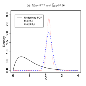
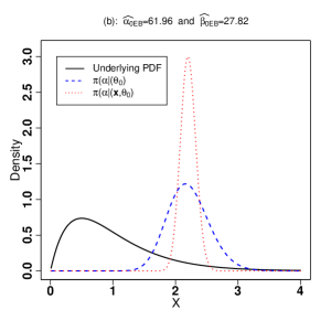
Figure 7.1: Schematic diagram for PDF of underlying, prior, and posterior when (a): $n=50$ and (b): $n=100$. Figure 7.1 shows the visual comparison between prior and posterior distributions when sample evidence are generated from ${\cal{G}}(\alpha=2,\beta=2)$ as underlying distribution for two data sets of sizes $n=50$ and $n=100$.

7.3 Credible interval

One common type of inference in frequentist statistics is confidence interval. The Bayesian analogue of confidence interval is known as credible interval and defined as follows.

Definition 7.3.1.

Given the observed sample evidence $\bm{x}=\{x_{1},\cdots,x_{n}\}$, the interval $(L,U)$ is a $100(1-\gamma)\%$ credible interval for unknown parameter $\theta$ if

$$P(L<\theta<U|\bm{x})=\int_{L}^{U}\pi(\theta|\bm{x})d\theta\geq 1-\gamma,$$ (7.19)

where $0<\gamma<1$.

Indeed, Definition 7.2 states that there is at least $100(1-\gamma)\%$ confidence that interval $(L,U)$ includes unknown parameter $\theta$. Figure 7.2 provides a schematic diagram for credible interval.

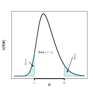
Figure 7.2: Schematic diagram for credible interval.

Example 16 Let $x_{1},x_{2},\cdots,x_{n}$ come independently from ${\cal{N}}(\mu,\sigma^{2})$ with known variance. By considering a conjugate prior ${\cal{N}}(\cdot|\mu_{0},\sigma_{0}^{2})$ for $\mu$, we recall from (7.5) that $\mu|\bm{x}$ follows a Gaussian distribution. Hence

$$\sqrt{\frac{n}{\sigma^{2}}+\frac{1}{\sigma_{0}^{2}}}\biggl{(}\mu-\frac{n^{-1}\sigma^{2}\mu_{0}+\sigma_{0}^{2}\bar{x}}{n^{-1}\sigma^{2}+\sigma_{0}^{2}}\biggr{)}\sim{\cal{N}}(0,1).$$ (7.20)

Therefore, $100(1-\gamma)\%$ credible interval for $\mu$ is given by

$$\frac{n^{-1}\sigma^{2}\mu_{0}+\sigma_{0}^{2}\bar{x}}{n^{-1}\sigma^{2}+\sigma_{0}^{2}}\pm z_{\gamma/2}\sqrt{\frac{n}{\sigma^{2}}+\frac{1}{\sigma_{0}^{2}}},$$ (7.21)

where $z_{\gamma/2}$ is the upper $\gamma/2$-quantile of the standard Gaussian distribution, that is, $P\bigl{(}Z>z_{\gamma/2}\bigr{)}=\gamma/2$ in which $Z\sim{\cal{N}}(0,1)$.

As it is seen from Example 7.3, for constructing credible interval, the upper and lower $\gamma/2$ of the posterior must be known. If the posterior gets complicated from the latter quantities cannot be found easily. In such cases, credible interval is constructed based on upper $\gamma/2$-quantile of the samples generated from the posterior. Let $\pi_{\gamma/2}$ denote the posterior’s upper $\gamma/2$-quantile, that is

$$\int_{\pi_{\gamma/2}}^{\infty}\pi(\theta|\bm{x})d\theta=\frac{\gamma}{2}.$$ (7.22)

Furthermore, suppose $\lceil{u}\rceil$ denotes the smallest integer value equal or greater than real value $u$ and $\theta_{(r)}$ is $r$th order statistic of sample $\{\theta_{1},\theta_{2},\cdots,\theta_{N}\}$ generated from posterior with PDF $\pi(\theta|\bm{x})$. When $N\rightarrow\infty$, then strong law of large numbers states that $\pi_{\gamma/2}\approx\theta_{(v)}$ where $v=\lceil{(1-\gamma/2)N}\rceil$. The definition below gives the empirical credible interval.

Definition 7.3.2.

Let $\{\theta_{1},\theta_{2},\cdots,\theta_{N}\}$, for large $N$, denote generated samples form posterior with PDF $\pi(\theta|\bm{x})$. A $100(1-\gamma)\%$ empirical credible interval for unknown parameter $\theta$ is then give by

$$\bigl{(}L_{e},U_{e}\bigr{)}=\bigl{(}\theta_{(v)},\theta_{(N-v)}\bigr{)},$$ (7.23)

where $v=\lceil{(1-\gamma/2)N}\rceil$.

Example 17 [continued]Recalling from Example 7.2, suppose we observed $n=200$ observations, represented as $\bm{x}=\bigl{\{}x_{1},x_{2},\cdots,x_{200}\bigr{\}}$ from ${\cal{G}}(\alpha=2,\beta=2)$. For known $\beta$, using the moment-based method described earlier in Example 7.2, we obtain $\bm{\theta}_{0}=\bigl{(}\widehat{\alpha_{0}}_{EB},\widehat{\beta_{0}}_{EB}\bigr{)}^{\top}=(62.179,30.083)^{\top}$. The corresponding posterior is given by

$$\pi\bigl{(}\alpha\big{|}\bm{x},\bm{\theta}_{0}\bigr{)}\propto \Bigl{[}\prod_{i=1}^{n}\frac{\beta^{\alpha}x_{i}^{\alpha-1}}{\Gamma(\alpha)}\exp\bigl{\{}-\beta x_{i}\bigr{\}}\Bigr{]}\frac{\beta_{0}^{\alpha_{0}}\alpha^{\alpha_{0}-1}}{\Gamma\bigl{(}\alpha_{0}\bigr{)}}\exp\bigl{\{}-\beta_{0}\alpha\bigr{\}},$$

$$\propto \frac{\beta^{n\alpha}\alpha^{\alpha_{0}-1}}{\bigl{[}\Gamma(\alpha)\bigr{]}^{n}}\Bigl{[}\prod_{i=1}^{n}x_{i}\Bigr{]}^{\alpha-1}\exp\bigl{\{}-\beta_{0}\alpha\bigr{\}}.$$ (7.24)

In order to construct a 95% empirical credible interval for $\alpha$, we need to sample from posterior (7.3) using methods such as MH or ARS. Taking into account into the fact that $\widehat{\alpha_{0}}_{EB}=62.179$ and it is simple to see that the posterior (7.3) is log-concave for $\alpha_{0}\geq 1$. So, we proceed for simulating from this posterior using the ARS approach. Based on a sample of size 5000 generated from posterior (7.3), we obtain quantities $L_{e}=1.778$, $\hat{\alpha}_{B}=1.945$, and $U_{e}=2.121$. The scatterplot of generated samples as well as the latter quantities are shown in Figure 7.3.

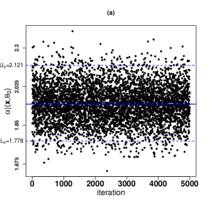
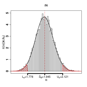
Figure 7.3: (a): the 95% empirical credible interval for parameter $\alpha$ based on a sample of $n=200$ realizations generated from ${\cal{G}}(\alpha=2,\beta=2)$ distribution and (b): histogram of the generated samples with fitted posterior $\pi\bigl{(}\alpha\big{|}\bm{x},\bm{\theta}_{0}\bigr{)}$. The R code for constructing the 95% empirical credible interval for $\alpha$ is given below.

⬇

1R> f.a <- function(x, beta, alpha0, beta0, y)

2+ {

3+ n=length(y); n*x*log(beta)-n*lgamma(x)+(alpha0-1)*log(x)+

4+ (x-1)*sum(y)-beta0*x

5+ }

6R> fprim.a <- function(x, beta, alpha0, beta0, y)

7+ {

8+ n=length(y); n*log(beta)-n*digamma(x)+(alpha0-1)/x+sum(y)-beta0

9+ }

10R> library(ars)

11R> set.seed(20240608)

12R> n <- 200; alpha <-2; beta <- 2

13R> y <- rgamma(n, shape = alpha, rate = beta)

14R> alpha0 <- beta*mean(y)^2/abs( beta*var(y) - mean(y) )

15R> beta0 <- alpha0/(beta*mean(y))

16R> N <- 5000 # number of generations

17R> M <- 0 # size of burn-in period

18R> theta <- rep(0, N)

19R> for(j in 1:N)

20+ {

21+ theta[j] <- ars(1, f.a, fprim.a, x = c(0.1, 4, 10, 30), m = 4,

22+ lb = TRUE, xlb = 0, ub = FALSE, beta = beta, alpha0 = alpha0,

23+ beta0 = beta0, y = log(y) )

24+ }

25R> Le <- quantile(theta[(M+1):N], 0.025)[[1]]

26R> Ue <- quantile(theta[(M+1):N], 0.975)[[1]]

27R> alphahat_B <- mean(theta)

28R> list("Lower_bound"=Le, "Bayes␣estimator"=alphahat_B, "Upper_bound"=Ue)

Chapter 8 Gibbs sampling

“Statistics is the science of information gathering, especially when the information arrives in little pieces instead of big ones.”

– Bradley Efron, Stanford University

This section has three parts. First, we describe the concept of Gibbs sampling as a general framework for generating independent samples from the given multivariate target distribution. Second, we discuss the situation that the Gibbs sampling is utilized to estimate the model’s unknown parameter(s) through the Bayesian paradigm.

8.1 Gibbs sampling in broad sense

The Gibbs sampling (or sampler) is an iterative Markov chain Monte Carlo (MCMC) sampling approach was developed by Geman and Geman (1984) for image reconstruction, but its application in statistical analyses were shown by Gelfand and Smith (1990). Assuming that we are at $t$th iteration of the Gibbs sampling and $\pi(\bm{x})$ denote the PDF of target distribution from which generating sample $\bm{x}=(x_{1},\cdots,x_{p})^{p}$ is of interest. For convenience, there follows a set of generic symbols as

$$\bm{x}^{(t)}=\bigl{(}{x}_{1}^{(t)},{x}_{2}^{(t)},\cdots,{x}_{p}^{(t)}\bigr{)},$$

$$\bm{x}_{i}^{(t)}[y]=\bigl{(}{x}_{1}^{(t)},\cdots,{x}_{i-1}^{(t)},y,{x}_{i+1}^{(t)},\cdots,{x}_{p}^{(t)}\bigr{)},$$

$$\bm{x}^{(t)}[-i]=\bigl{(}{x}_{1}^{(t)},\cdots,{x}_{i-1}^{(t)},{x}_{i+1}^{(t)},\cdots,{x}_{p}^{(t)}\bigr{)}.$$ (8.1)

It is noteworthy that sampling from a $p$-dimensional distribution using the methods such as MH or AMH discussed earlier may involve undesired computational burden. In such cases, the Gibbs sampling technique that works efficiently is becoming increasingly popular in a wide range of applications. Indeed, each Gibbs sampling scheme works by generating sample from conditional distribution of vector $\bm{x}=(x_{1},\cdots,x_{p})^{p}$ that is known in the literature as the full conditional. For example, for generating $\bm{x}=(x_{1},\cdots,x_{p})^{p}$ form target PDF $\pi(\bm{x})$, the conditional distribution (or PDF) $\pi\bigl{(}x_{i}\big{|}\bm{x}[-i]\bigr{)}$ is called full conditional of $x_{i}$ (for $i=1,\cdots,p$). It is proved (Geman and Geman, 1984) that, after burn-in period (Roberts and Smith, 1994), the generated sample comes from the target distribution whose PDF is $\pi(\bm{x})$. Each Gibbs sampling technique is summarized by the following algorithm.

Algorithm 5 Gibbs sampling Technique

1:Set $t=1$, read $M$ (burn-in period), $N$ (total number of iterations), and

2:initiate algorithm with randomly selected sample $\bm{x}^{(0)}$;

3:while $t\leq N$ do

4:     while $i\leq p$ do

5:         Generate sample $y$ from full conditional with PDF $\pi\bigl{(}x^{(t)}_{i}\big{|}\bm{x}^{(t-1)}[-i]\bigr{)}$;

6:         Set $\bm{x}^{(t+1)}\leftarrow\bm{x}_{i}^{(t)}[y]$ (that is

7:         ${x}_{i}^{(t+1)}\leftarrow y$ and $\bm{x}^{(t+1)}[-i]\leftarrow\bm{x}^{(t)}[-i]$);

8:         Set $i\leftarrow i+1$;      

9:     end

10:     Set $t\leftarrow t+1$;

11:end

12:Sequence $\bigl{\{}\bm{x}_{M},\bm{x}_{M+1},\cdots,\bm{x}_{N}\bigr{\}}$ is a sample of size $N-M+1$ from

13:target distribution with PDF $\pi\bigl{(}\bm{x})$.

Example 18 Let $\bm{X}=\bigl{(}X_{1},X_{2}\bigr{)}^{\top}$ follows a bivariate Gaussian distribution with PDF

$$\pi\bigl{(}\bm{x}\big{|}\rho\bigr{)}=\frac{1}{2\pi\sqrt{1-\rho^{2}}}\exp\Bigl{\{}-\frac{x_{1}^{2}+x_{2}^{2}-2\rho x_{1}x_{2}}{2(1-\rho^{2})}\Bigr{\}}.$$ (8.2)

where $\bm{x}=\bigl{(}x_{1},x_{2}\bigr{)}^{\top}$ and $-1<\rho<1$. Since we have just two variables $X_{1}$ and $X_{2}$, so for simulating from $\bm{X}$ using the Gibbs sampling technique, we need to simulate from full conditionals $X_{1}\big{|}\bigl{(}X_{2},\rho\bigr{)}$ and $X_{2}\big{|}\bigl{(}X_{1},\rho\bigr{)}$. It can be easily seen that

$$\pi\bigl{(}x_{1}\big{|}x_{2},\rho\bigr{)}\propto\exp\Bigl{\{}-\frac{x_{1}^{2}-2\rho x_{1}x_{2}}{2(1-\rho^{2})}\Bigr{\}}.$$ (8.3)

Since $x_{1}^{2}-2\rho x_{1}x_{2}=(x_{1}-\rho x_{2})^{2}-(\rho x_{2})^{2}$, then it follows that

$$\pi\bigl{(}x_{1}\big{|}x_{2},\rho\bigr{)}\propto\exp\Bigl{\{}-\frac{(x_{1}-\rho x_{2})^{2}}{2(1-\rho^{2})}\Bigr{\}}.$$ (8.4)

This means that $X_{1}\big{|}\bigl{(}X_{2},\rho\bigr{)}\sim{\cal{N}}(\rho x_{2},1-\rho^{2})$. Likewise, we can write $X_{2}\big{|}\bigl{(}X_{1},\rho\bigr{)}\sim{\cal{N}}(\rho x_{1},1-\rho^{2})$. Hence, given $\bm{x}^{(0)}=\bigl{(}x^{(0)}_{1},x^{(0)}_{2}\bigr{)}^{\top}$, for simulating a sample of $n=3000$ observations when $M=2000$, the steps of the Gibbs sampling given in Algorithm (5) are as follows.

1. Set $t=1$, and generate $\bm{x}^{(0)}=\bigl{(}x^{(0)}_{1},x^{(0)}_{2}\bigr{)}^{\top}$ in which $x^{(0)}_{1}\sim{\cal{N}}\bigl{(}0,1-\rho^{2}\bigr{)}$ and $x^{(0)}_{2}\sim{\cal{N}}\bigl{(}0,1-\rho^{2}\bigr{)}$;

2. Set $t=0$;

3. Simulate $x^{(t+1)}_{1}$ from the full conditional $x^{(t+1)}_{1}\big{|}\bigl{(}x^{(t)}_{2},\rho\bigr{)}\sim{\cal{N}}\bigl{(}\rho x^{(t)}_{2},1-\rho^{2}\bigr{)}$;

4. Having $x^{(t+1)}_{1}$, simulate $x^{(t+1)}_{2}$ from the full conditional $x^{(t+1)}_{2}\big{|}\bigl{(}x^{(t)}_{1},\rho\bigr{)}\sim{\cal{N}}\bigl{(}\rho x^{(t+1)}_{1},1-\rho^{2}\bigr{)}$;

5. If $t=5000$, then go to the next step, otherwise $t\leftarrow t+1$ and return step 3;

6. Sequence $\bigl{\{}\bm{x}_{2001},\bm{x}_{2002},\cdots,\bm{x}_{5000}\bigr{\}}$ constitutes a sample of size 3000 from target distribution with PDF $\pi\bigl{(}\bm{x}\big{|}\rho\bigr{)}$.

The associated R code for generating 3000 realizations from ${\cal{N}}_{2}(\mu_{1}=0,\mu_{2}=0,\sigma_{1}^{2}=1,\sigma_{2}^{2}=1,\rho=0.50)$ is given as follows.

⬇

1R > set.seed(20240520)

2R > N <- 5000 # number of generations

3R > M <- 2000 # size of burn-in period

4R > rho <- 0.5

5R > X <- matrix(0, nrow = N, ncol = 2)

6R > sigma1 <- sigma2 <- 1

7R > Sigma <- matrix( c(1, rho*sigma1*sigma2, rho*sigma1*sigma2, 1), 2, 2)

8R > X[1, ] <- rnorm (2, mean = 0, sd = 1 - rho^2) # intitial generation

9R > j <- 1

10R > while(j < N)

11+ {

12+ X[j + 1, 1] <- rnorm (1, mean = rho*sqrt(Sigma[1,1]/Sigma[2,2])*X[j , 2],

13+ sd = 1 - rho^2)

14+ X[j + 1, 2] <- rnorm (1, mean = rho*sqrt(Sigma[2,2]/Sigma[1,1])*X[j + 1, 1],

15+ sd= 1 - rho^2)

16+ j <- j + 1

17+ }

18R > plot(X[(N-M+1):N,])

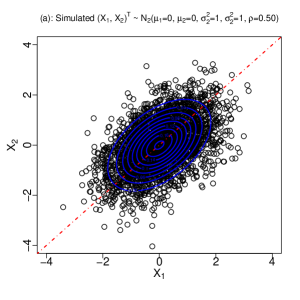
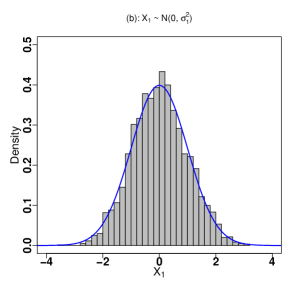
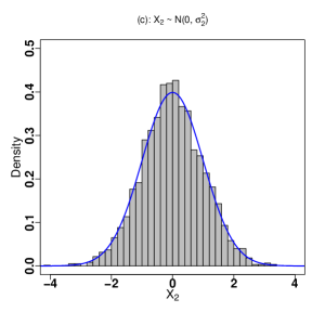
Figure 8.1: (a): Scatterplot with fitted contours based on 3000 samples generated from ${\cal{N}}_{2}(\mu_{1}=0,\mu_{2}=0,\sigma_{1}^{2}=1,\sigma_{2}^{2}=1,\rho=0.50)$, (b): histogram of generated samples from marginal $X_{1}$, and (c): histogram of generated samples from marginal $X_{2}$.

8.2 Gibbs sampling in Bayesian paradigm

Herein, we show how a Gibbs sampling technique described in the previous section can be used for computing the Bayesian estimator of the unknown parameter $\bm{\theta}=(\theta_{1},\cdots,\theta_{p})^{\top}$. Notice that, based on random sample $\{x_{1},\cdots,x_{n}\}$ following a distribution with PDF $f(.|\bm{\theta})$, the Bayes estimator of $\bm{\theta}$ usually becomes the mean of the posterior defined as

$$E\bigl{[}\bm{\theta}\big{|}\bm{x}\bigr{]}=\int_{\mathbb{R}^{p}}\bm{\theta}\pi(\bm{\theta}|\bm{x})d\bm{\theta}.$$ (8.5)

Computing integration (8.5) may involve huge computational burden especially when number of parameters $p$, is large. The law of large numbers guarantees that the sample mean converges with probability one to the population mean when sample size is sufficiently large, that is

$$\hat{\bm{\theta}}=\underset{N\rightarrow\infty}{\operatorname{limit}}\leavevmode\nobreak\ \frac{\bm{\theta}^{(1)}+\cdots+\bm{\theta}^{(N)}}{N}=E\bigl{[}\bm{\theta}\big{|}\bm{x}\bigr{]}.$$

Hence, if we could generate sample enough from the posterior $\pi(\bm{\theta}|\bm{x})$, then $\bm{\theta}$ can be estimated via $\hat{\bm{\theta}}$ in which $\{\bm{\theta}^{(1)},\cdots,\bm{\theta}^{(N)}\}$ is generated from posterior $\pi(\bm{\theta}|\bm{x})$ when $N$ is sufficiently large (here $\bm{\theta}^{(i)}$ denotes the $i$th sample generated from posterior $\pi(\bm{\theta}|\bm{x})$). Generating sample from the target distribution (that is here $\pi(\bm{\theta}|\bm{x})$) using the MCMC techniques described in the previous section appears to be challenging when $p$ is large. In such cases, the Gibbs sampling is guaranteed to work well.

It should be noted that since in each Bayesian framework the unknown parameter $\bm{\theta}=(\theta_{1},\cdots,\theta_{p})^{\top}$ itself is a random variable, in addition of the model’s variables, herein we must consider an extra number of $p$ additional full conditionals within a Gibbs sampler schemes. For instance, recalling from the Example (3), we must consider three full conditionals given by variables $X_{1}\big{|}X_{2},\rho$, $X_{2}\big{|}X_{1},\rho$, and $\rho\big{|}X_{1},X_{2}$. In what follows, we consider the foregoing example when Bayesian inference on $\rho$ is desired.

Example 19 Let ${\underline{\bm{x}}}=\{\bm{x}_{1},\bm{x}_{2},\cdots,\bm{x}_{n}$} account for a sequence of $n$ independent observations in which $\bm{x}_{i}=\bigl{(}x_{i1},x_{i2}\bigr{)}^{\top}$. Furthermore, assume $\bm{x}_{i}$ (for $i=1,2,\cdots,n$) follows a bivariate Gaussian distribution with PDF given by

$$\pi\bigl{(}\bm{x}_{i}\big{|}\bm{\theta}\bigr{)}=\frac{1}{2\pi\sigma_{1}\sigma_{2}\sqrt{1-\rho^{2}}}\exp\Bigl{\{}-\frac{1}{2(1-\rho^{2})}\Bigl{[}\Bigl{(}\frac{x_{i1}}{\sigma_{1}}\Bigr{)}^{2}+\Bigl{(}\frac{x_{i2}}{\sigma_{2}}\Bigr{)}^{2}-2\rho\frac{x_{i1}x_{i2}}{\sigma_{1}\sigma_{2}}\Bigr{]}\Bigr{\}},$$ (8.6)

where $\bm{\theta}=(\sigma_{1},\sigma_{2},\rho)^{\top}$ is the unknown parameter vector. Using a reparameterization $\bm{\theta}=(\theta_{1},\theta_{2},\theta_{3})^{\top}$ in which $\theta_{1}=\sigma_{1}/\sigma_{2}$, $\theta_{2}=\sigma_{1}\sigma_{2}\sqrt{1-\rho^{2}}$, and $\theta_{3}=\rho$, the bivariate Gaussian PDF is rewritten as by

$$\pi\bigl{(}\bm{x}_{i}\big{|}\bm{\theta}\bigr{)}=\frac{1}{2\pi\theta_{2}}\exp\Bigl{\{}-\frac{1}{2(1-\theta_{3}^{2})^{1/2}\theta_{2}}\Bigl{[}\frac{x^{2}_{i1}}{\theta_{1}}+\theta_{1}x^{2}_{i2}-2\theta_{3}x_{i1}x_{i2}\Bigr{]}\Bigr{\}}.$$ (8.7)

For computing the Bayesian estimator of $\bm{\theta}$, we first note that

$$\pi\bigl{(}\rho\big{|}{\underline{\bm{x}}}\bigr{)} \propto\prod_{i=1}^{n}\pi\bigl{(}\bm{x}_{i}\big{|}\bm{\theta})\pi(\bm{\theta}\bigr{)}.$$ (8.8)

The marginals of joint prior $\pi(\bm{\theta})$ are assumed to be independent, that is, $\pi(\bm{\theta})=\pi(\theta_{1})\pi(\theta_{2})\pi(\theta_{3})$. Also, we consider gamma prior for both of $\theta_{1}$, inverse gamma prior for $\theta_{2}$, and an uniform on (-1,1) prior for $\theta$ represented, respectively, as follows.

$$\pi(\theta_{1}\big{|}a_{1},b_{1}) =\frac{b_{1}^{a_{1}}\theta_{1}^{a_{1}-1}}{\Gamma(a_{1})}\exp\bigl{\{}-b_{1}\theta_{1}\bigr{\}},\leavevmode\nobreak\ \leavevmode\nobreak\ \theta_{1}>0,$$

$$\pi(\theta_{2}\big{|}a_{2},b_{2}) =\frac{b_{2}^{a_{2}}\theta_{2}^{-a_{2}-1}}{\Gamma(a_{2})}\exp\bigl{\{}-\frac{b_{2}}{\theta_{2}}\bigr{\}},\leavevmode\nobreak\ \leavevmode\nobreak\ \theta_{2}>0,$$

$$\pi(\theta_{3}) =\frac{1}{2},\leavevmode\nobreak\ \leavevmode\nobreak\ -1<\theta_{3}<1.$$ (8.9)

We note that, here we consider above priors just for the simplicity of computations. It follows that

$$\pi\bigl{(}\bm{\theta}\big{|}{\underline{\bm{x}}}\bigr{)}\propto \frac{1}{\theta_{2}^{n}}\exp\Bigl{\{}-\frac{1}{2\theta_{2}\sqrt{1-\theta_{3}^{2}}}\Bigl{[}\frac{\sum_{i=1}^{n}x_{i1}^{2}}{\theta_{1}}+\theta_{1}\sum_{i=1}^{n}x_{i2}^{2}-2\theta_{3}\sum_{i=1}^{n}x_{i1}x_{i2}{}\Bigr{]}\Bigr{\}}$$

$$\times\frac{b_{1}^{a_{1}}\theta_{1}^{a_{1}-1}}{\Gamma(a_{1})}\exp\bigl{\{}-b_{1}\theta_{1}\bigr{\}}\times\frac{b_{2}^{a_{2}}\theta_{2}^{-a_{2}-1}}{\Gamma(a_{2})}\exp\bigl{\{}-\frac{b_{2}}{\theta_{2}}\bigr{\}}\times\frac{1}{2}$$ (8.10)

We note that, herein, the model’s variables are $\theta_{1}$, $\theta_{2}$, and $\theta_{3}$. So, by dropping out all terms that do not depend on $\theta_{1}$ from the posterior (8.2), then the full conditional ${\theta}_{1}\big{|}(\theta_{2},\theta_{3},{\underline{\bm{x}}})$, after some algebra, is shown to be

$$\pi\bigl{(}{\theta}_{1}\big{|}\theta_{2},\theta_{3},{\underline{\bm{x}}}\bigr{)}\propto \theta_{1}^{-a_{1}-1}\exp\Bigl{\{}-\frac{\theta_{1}}{2}\Bigl{[}2b_{1}+\frac{\sum_{i=1}^{n}x_{i2}^{2}}{\theta_{2}(1-\theta_{3})^{1/2}}\Bigr{]}-\frac{1}{2\theta_{1}}\Bigl{[}\frac{\sum_{i=1}^{n}x_{i1}^{2}}{\theta_{2}(1-\theta_{3})^{1/2}}\Bigr{]}\Bigr{\}}.$$ (8.11)

Comparing the RHSs of (8.11) and (2.7), it turns out that (8.11) is the core of a ${\cal{GIG}}(a,b,c)$ PDF where $a=a_{1}$, $b=2b_{1}+\sum_{i=1}^{n}x_{i2}^{2}/\bigl{[}\theta_{2}(1-\theta_{3})^{1/2}\bigr{]}$, $c=\sum_{i=1}^{n}x_{i1}^{2}/\bigl{[}\theta_{2}(1-\theta_{3})^{1/2}\bigr{]}$. So,

$${\theta}_{1}\big{|}(\theta_{2},\theta_{3},{\underline{\bm{x}}})\sim{\cal{GIG}}\Bigl{(}a_{1},2b_{1}+\sum_{i=1}^{n}x_{i2}^{2}/\bigl{[}\theta_{2}(1-\theta_{3})^{1/2}\bigr{]},\sum_{i=1}^{n}x_{i1}^{2}/\bigl{[}\theta_{2}(1-\theta_{3})^{1/2}\bigr{]}\Bigr{)}.$$ (8.12)

Likewise, we can see that the full conditional ${\theta}_{2}\big{|}(\theta_{1},\theta_{3},{\underline{\bm{x}}})$ follows an inverse gamma distribution. We have

$${\theta}_{2}\big{|}(\theta_{1},\theta_{3},{\underline{\bm{x}}})\sim {\cal{IG}}\biggl{(}n+a_{2},b_{2}+\frac{1}{2\theta_{2}(1-\theta_{3})^{1/2}}$$

$$\times\Bigl{[}\theta^{-1}_{1}\sum_{i=1}^{n}x_{i1}^{2}+\theta_{1}\sum_{i=1}^{n}x_{i2}^{2}-2\theta_{3}\sum_{i=1}^{n}x_{i1}x_{i2}\Bigr{]}\biggr{)},$$ (8.13)

and finally

$${\theta}_{3}\big{|}(\theta_{1},\theta_{2},{\underline{\bm{x}}})\propto\exp\biggl{\{}-\frac{1}{2\theta_{2}\sqrt{1-\theta_{3}^{2}}}\Bigl{[}\theta_{1}^{-1}\sum_{i=1}^{n}x_{i1}^{2}+\theta_{1}\sum_{i=1}^{n}x_{i2}^{2}-2\theta_{3}\sum_{i=1}^{n}x_{i1}x_{i2}\Bigr{]}\biggr{\}}.$$ (8.14)

As it is seen, the full conditional ${\theta}_{3}\big{|}(\theta_{1},\theta_{2},{\underline{\bm{x}}})$ has no closed form. Hence, we can use the MH within Gibbs sampling technique. Recall from Subsection 1.1, considering a symmetric uniform proposal on (-1,1), the transition probability $p\bigl{(}\theta_{3(n)}\rightarrow\theta_{3(n+1)}\bigr{)}=\min\bigl{\{}1,\exp\{R_{1}-R_{2}\}\bigr{\}}$, is

$$R_{1}=-\frac{1}{2\theta_{2}\sqrt{1-\theta_{3(n+1)}^{2}}}\Bigl{[}\theta_{1}^{-1}\sum_{i=1}^{n}x_{i1}^{2}+\theta_{1}\sum_{i=1}^{n}x_{i2}^{2}-2\theta_{3(n+1)}\sum_{i=1}^{n}x_{i1}x_{i2}{}\Bigr{]}$$

$$R_{2}=-\frac{1}{2\theta_{2}\sqrt{1-\theta_{3(n)}^{2}}}\Bigl{[}\theta_{1}^{-1}\sum_{i=1}^{n}x_{i1}^{2}+\theta_{1}\sum_{i=1}^{n}x_{i2}^{2}-2\theta_{3(n)}\sum_{i=1}^{n}x_{i1}x_{i2}{}\Bigr{]}$$ (8.15)

In what follows, we give the steps for computing Bayesian estimation of ${\bm{\theta}}$.

1. Read $N,M,a_{1},b_{1},a_{2},b_{2}$, and suggest $\bm{\theta}^{(0)}=\bigl{(}\theta^{(0)}_{1},\theta^{(0)}_{2},\theta^{(0)}_{3}\bigr{)}^{\top}$ arbitrarily;

2. Set $t=0$;

3. Simulate $\theta^{(t+1)}_{1}$ from the full conditional $\theta^{(t+1)}_{1}\big{|}\bigl{(}\theta^{(t)}_{2},\theta^{(t)}_{3},{\underline{\bm{x}}}\bigr{)}$ that follows

   $${\cal{GIG}}\Bigl{(}a_{1},2b_{1}+\sum_{i=1}^{n}x_{2i}^{2}/\bigl{[}\theta^{(t)}_{2}(1-\theta^{(t)}_{3})^{1/2}\bigr{]},\sum_{i=1}^{n}x_{1i}^{2}/\bigl{[}\theta^{(t)}_{2}(1-\theta^{(t)}_{3})^{1/2}\bigr{]}\Bigr{)};$$

4. Having $\theta^{(t+1)}_{1}$, simulate $\theta^{(t+1)}_{2}$ from the full conditional $\theta^{(t)}_{2}\big{|}\bigl{(}\theta^{(t+1)}_{1},\theta^{(t)}_{3},{\underline{\bm{x}}}\bigr{)}$ that follows

   $${\cal{GIG}}\biggl{(}n+a_{2},2b_{2},\Bigl{[}\frac{1}{\theta^{(t+1)}_{1}}\sum_{i=1}^{n}x_{i1}^{2}+\theta^{(t+1)}_{1}\sum_{i=1}^{n}x_{i2}^{2}-2\theta^{(t)}_{3}\sum_{i=1}^{n}x_{i1}x_{i2}\Bigr{]}$$

   $$\Bigl{[}\theta^{(t)}_{2}(1-\theta^{(t)}_{3})^{1/2}\Bigr{]}^{-1}\biggr{)};$$

5. Having $\theta^{(t+1)}_{1}$ and $\theta^{(t+1)}_{2}$, simulate $\theta^{(t+1)}_{3}$ from the full conditional $\theta^{(t)}_{3}\big{|}\bigl{(}\theta^{(t+1)}_{2},\theta^{(t)}_{3},{\underline{\bm{x}}}\bigr{)}$ using MH-within-Gibbs sampling technique as follows.

   1. Set $k=0$, $K=100$, and choose the initial state as $y_{0}\sim{\cal{U}}(-1,1)$;

   2. Generate $y^{(k+1)}\sim{\cal{U}}(-1,1)$

   3. Compute $p\bigl{(}y^{(k)}\rightarrow y^{(k+1)}\bigr{)}=\min\bigl{\{}1,\exp\{R_{1}-R_{2}\}\bigr{\}}$ where

      $$R_{1}=-\frac{1}{2\theta^{(t+1)}_{2}\sqrt{1-\bigl{(}y^{(k+1)}\bigr{)}^{2}}}\Bigl{[}\frac{1}{\theta^{(t+1)}_{1}}\sum_{i=1}^{n}x_{i1}^{2}+\theta_{1}\sum_{i=1}^{n}x_{i1}^{2}-2y^{(k+1)}\sum_{i=1}^{n}x_{i1}x_{i2}\Bigr{]}$$

      and

      $$R_{2}=-\frac{1}{2\theta^{(t+1)}_{2}\sqrt{1-\bigl{(}y^{(k)}\bigr{)}^{2}}}\Bigl{[}\frac{1}{\theta^{(t+1)}_{1}}\sum_{i=1}^{n}x_{i1}^{2}+\theta^{(t+1)}_{1}\sum_{i=1}^{n}x_{i2}^{2}-2y^{(k)}\sum_{i=1}^{n}x_{i1}x_{i2}\Bigr{]}$$

   4. Generate $u\sim{\text{U}}(0,1)$;

   5. If $u<p\bigl{(}y^{(k)},y^{(k+1)}\bigr{)}$ then $y^{(k)}\rightarrow y^{(k+1)}$ and $k\rightarrow k+1$;

   6. Repeat algorithm from step (b);

   7. If $k=K$ then $y^{(k+1)}\rightarrow\theta^{(t+1)}_{3}$ and stop the algorithm.

6. If $t=N$, then go to the next step, otherwise $t+1\rightarrow t$ and return step 3;

7. The Bayesian estimator $\hat{\bm{\theta}}_{B}$, is the average of $N-M+1$ samples, that is, $\bm{\theta}^{(M+1)},\bm{\theta}^{(M+2)},\cdots,\bm{\theta}^{(M+N)}$ generated from target PDF $\pi\bigl{(}\bm{\theta}|{\underline{\bm{x}}}\bigr{)}$.

We note that, in practice, hyperparameters $a_{1},b_{1},a_{2}$ and $b_{2}$ are determined based on experimenter’s belief or the empirical Bayes. If sample size is small, then the improper Jeffreys prior is suggested. It is noteworthy that for simulating from GIG distribution, one can use the method proposed by Hörmann and Leydold (2014).

The pertaining R code for implementing example above is given as follows. To this end, a sample of $N=5000$ realizations have been generated from a zero-mean bivariate Gaussian when $\sigma_{1}=0.5$, $\sigma_{2}=1$, and $\rho=-0.75$. The output of the Gibbs sampler is displayed in Figure 8.2.

⬇

1R > set.seed(20240522)

2R > library(MASS)

3R > library(GIGrvg)

4R > n <- 5000 # sample size

5R > Mu <- c(0, 0)

6R > X <- matrix(0, nrow = n, ncol = 2)

7R > sigma1 <- 1; sigma2 <- .5; rho <- -0.75

8R > Sigma <- matrix( c(sigma1^2,rho*sigma1*sigma2,rho*sigma1*sigma2,sigma2^2), 2, 2)

9R > X <- mvrnorm(n, Mu, Sigma)

10R > n.sim <- 5000 # number of Gibbs sampling iterations

11R > n.burn <- 2000 # length of burn-in period

12R > K <- 100 # number of MH algorithm iterations

13R > theta3i <- rep(0, K)

14R > a1 <- 0.5; b1<- 0.5; a2 <- 0.5; b2 <- 0.5;

15R > theta <- matrix(0, nrow = n.sim, ncol = 3)

16R > theta[1, ] <- c(1, 1, 0.75)

17R > sx1 <- sum(X[, 1]^2); sx2 <- sum(X[, 2]^2); sx12 <- sum(X[, 1]*X[, 2])

18R > j <- 1

19R > while(j < n.sim)

20+ {

21+ c0 <- ( theta[j, 2]*sqrt( 1 - theta[j, 3]^2 ) )

22+ rate1 <- function(x) (sx1/theta[j, 1] + theta[j, 1]*sx2 - 2*x*sx12)/sqrt(1-x^2)

23+ theta[j + 1, 1] <- rgig(n = 1, lambda = a1, chi = sx1/c0, psi = 2*b1 + sx2/c0 )

24+ theta[j + 1, 2] <- 1/rgamma(n=1, shape=n + a2, rate=rate1(theta[j, 3])/2 + b2 )

25# start of MH-within-Gibbs sampling for sampling

26# from full conditional of theta3

27+ theta3i[1] <- runif(1, -1, 1)

28+ for(k in 2:K)

29+ {

30+ theta3.n <- runif(1, -1, 1)

31+ dif <- -( rate1(theta3.n) - rate1(theta3i[k - 1]) )/(2*theta[j + 1, 2])

32+ if( runif(1) < exp( dif ) )

33+ {

34+ theta3i[k] <- theta3.n # theta3.n is accepted

35+ }else{

36+ theta3i[k] <- theta3i[ k - 1] # theta3.n is rejected

37+ }

38+ }

39# start of MH-within-Gibbs sampling for sampling

40# from full conditional of theta3

41+ theta[j + 1, 3] <- theta3i[k]

42+ j <- j + 1

43+ }

44R > theta.hat <- apply(theta[(n.sim - n.burn + 1):n.sim, ], 2, mean)

45R > rho <- theta.hat[3] #estimator of rho

46R > sigma1 <- sqrt(theta.hat[1]*theta.hat[2]/sqrt(1-rho.hat^2)) #estimator of sigma1

47R > sigma2 <- sigma1.hat/theta.hat[1] #estimator of sigma2

Figure 8.2: Scatterplot of 5000 samples generated from full conditionals: (a) ${\theta}_{1}\big{|}(\theta_{2},\theta_{3},{{\bm{x}}})$, (b): ${\theta}_{2}\big{|}(\theta_{1},\theta_{3},{{\bm{x}}})$, and (c): ${\theta}_{3}\big{|}(\theta_{1},\theta_{2},{{\bm{x}}})$.

Example 20 Suppose response variable $Y$ depends linearly on independent variable (covariate) $X$ through a simple linear model as

$$y_{i}= \beta_{0}+\beta_{1}x_{i}+\epsilon_{i};\leavevmode\nobreak\ \leavevmode\nobreak\ i=1,2,3,\cdots,n.$$ (8.16)

Recording $n$ measurements on $Y$ represented as $y_{1},y_{2},y_{3},\cdots,y_{n}$ at the corresponding levels of covariate $X$ shown by $x_{1},x_{2},\cdots,x_{n}$, the focus is placed on estimating the regression coefficients $\beta_{0}$ and $\beta_{1}$ through the Bayesian approach. Herein, $\epsilon_{i}$s are the simple linear model’s theoretical errors, independently (that is, ${\text{cov}}\bigl{(}\epsilon_{i},\epsilon_{j}\bigr{)}=0$ for $i\neq j=1,2,3,\cdots,n$) assumed to follow ${\cal{N}}\bigl{(}0,\sigma^{2}\bigr{)}$. Of course the skewed Student’s $t$ (Teimouri et al., 2020) and $\alpha$-stable (Nolan and Ojeda-Revah, 2013) may be reasonable candidates for distribution of theoretical error in presence of outliers that yield more robust estimation of ${\bm{\beta}}=(\beta_{0},\beta_{1})^{\top}$ than the Gaussian one. It is known that the least-square (LS) estimator $\hat{\bm{\beta}}_{ls}$ and ML estimator $\hat{\bm{\beta}}_{ml}$, of the regression coefficients $\bm{\beta}$ are the same and given by

$$\hat{{\beta}_{1}}_{ML}=\hat{{\beta}_{1}}_{LS} ={\frac{\sum_{i=1}^{n}(x_{i}-{\bar{x}})(y_{i}-{\bar{y}})}{\sum_{i=1}^{n}(x_{i}-{\bar{x}})^{2}}},$$

$$\hat{{\beta}_{0}}_{ML}=\hat{{\beta}_{0}}_{LS} ={\bar{y}}-\hat{{\beta}_{0}}_{ML}\times\bar{x},$$ (8.17)

where $\bar{x}=\bigl{(}x_{1}+x_{2}+\cdots+x_{n}\bigr{)}/n$. Assuming independent Gaussian priors for elements of $\bm{\beta}$ and a mutually independent conjugate inverse gamma prior for $\delta=\sigma^{2}$ as

$$\pi(\beta_{0})= {\cal{N}}\bigl{(}\beta_{0}\big{|}\mu_{0},\sigma^{2}_{0}\bigr{)},$$

$$\pi(\beta_{1})= {\cal{N}}\bigl{(}\beta_{1}\big{|}\mu_{1},\sigma^{2}_{1}\bigr{)},$$

$$\pi(\delta)= {\cal{IG}}\Bigl{(}\delta\Big{|}\frac{a_{0}}{2},\frac{b_{0}}{2}\Bigr{)}.$$

It follows that

$$\pi(\bm{\theta}|\bm{y},\bm{x})= L\bigl{(}\bm{\theta}\big{|}\bm{y},\bm{x}\bigr{)}\pi(\beta_{0})\pi(\beta_{1})\pi(\delta)$$

$$\propto \frac{1}{\delta^{\frac{n}{2}}}\exp\Bigl{\{}-\frac{1}{2\delta}\sum_{i=1}^{n}\bigl{(}y_{i}-\beta_{0}-\beta_{1}x_{i}\bigr{)}^{2}\Bigr{\}}\frac{1}{\sqrt{2\pi\sigma^{2}_{0}}}\exp\Bigl{\{}-\frac{\bigl{(}\beta_{0}-\mu_{0}\bigr{)}^{2}}{2\sigma^{2}_{0}}\Bigr{\}}$$

$$\times\frac{1}{\sqrt{2\pi\sigma^{2}_{1}}}\exp\Bigl{\{}-\frac{\bigl{(}\beta_{1}-\mu_{1}\bigr{)}^{2}}{2\sigma^{2}_{1}}\Bigr{\}}\Bigl{(}\frac{b_{0}}{2}\Bigr{)}^{\frac{a_{0}}{2}}\frac{\delta^{-\frac{a_{0}}{2}-1}}{\Gamma\bigl{(}\frac{a_{0}}{2}\bigr{)}}\exp\Bigl{\{}-\frac{b_{0}}{2\delta}\Bigr{\}},$$ (8.18)

where $\delta=\sigma^{2}$ and $\bm{\theta}=({\beta}_{0},{\beta}_{1},\delta)^{\top}$. Then more algebra shows

$$\pi\bigl{(}{\beta}_{0}\big{|}\bm{y},\bm{x},\bm{\theta}_{(-\beta_{0})}\bigr{)}={\cal{N}}\biggl{(}{\beta}_{0}\bigg{|}D_{0}\biggl{[}\frac{\mu_{0}}{\sigma^{2}_{0}}+\frac{\sum_{i=1}^{n}\bigl{(}y_{i}-\beta_{1}x_{i}\bigr{)}}{\sigma^{2}}\biggr{]},D_{0}\biggr{)},$$ (8.19)

and

$$\pi\bigl{(}{\beta}_{1}\big{|}\bm{y},\bm{x},\bm{\theta}_{(-\beta_{1})}\bigr{)}={\cal{N}}\biggl{(}{\beta}_{1}\bigg{|}D_{1}\biggl{[}\frac{\mu_{1}}{\sigma^{2}_{1}}+\frac{\sum_{i=1}^{n}x_{i}\bigl{(}y_{i}-\beta_{0}\bigr{)}}{\sigma^{2}}\biggr{]},D_{1}\biggr{)},$$ (8.20)

where $D_{0}=\sigma_{0}^{2}\delta/\bigl{(}n\sigma_{0}^{2}+\delta\bigr{)}$ and $D_{1}=\sigma_{1}^{2}\delta/\bigl{(}\sigma_{1}^{2}\sum_{i=1}^{n}x^{2}_{i}+\delta\bigr{)}$. Furthermore, by considering transformation $\delta=\sigma^{2}$, it can be seen easily that

$$\pi\bigl{(}{\delta}\big{|}\bm{y},\bm{x},\bm{\theta}_{(-\bm{\beta})}\bigr{)}={\cal{IG}}\biggl{(}\delta\bigg{|}\frac{a_{0}+n}{2},\frac{a_{0}+\sum_{i=1}^{n}\bigl{(}y_{i}-{x}_{i}{\beta}\bigr{)}^{2}}{2}\biggr{]}\biggr{)}.$$ (8.21)

Applying a monotone transformation such used as above is a common trick in each Bayesian paradigm to yield a conjugate prior. Finally, the simple reverse transformation gives back the Bayesian estimator of $\sigma$. There follows the steps for computing Bayesian estimation of ${\bm{\theta}}$.

1. Read $N,M$, determine hyperparameters $\mu_{0},\mu_{1},\sigma_{0},\sigma_{1},a_{0},b_{0}$, and propose $\bm{\theta}^{(0)}=\bigl{(}\beta^{(0)}_{0},\beta^{(0)}_{1},\delta^{(0)}\bigr{)}^{\top}$;

2. Set $t=0$;

3. Simulate $\beta^{(t+1)}_{0}$ from the full conditional $\beta_{0}\big{|}\bigl{(}{\bm{y}},{\bm{x}},\bm{\theta}_{(-{\beta}_{0})}\bigr{)}$ that follows

   $${\cal{N}}\biggl{(}D^{(t)}_{0}\biggl{[}\frac{\mu_{0}}{\sigma^{2}_{0}}+\frac{\sum_{i=1}^{n}\bigl{(}y_{i}-\beta^{(t)}_{1}x_{i}\bigr{)}}{\delta^{(t)}}\biggr{]},D^{(t)}_{0}\biggr{)},$$

   where $D^{(t)}_{0}=\sigma_{0}^{2}\delta^{(t)}/\bigl{(}n\sigma_{0}^{2}+\delta^{(t)}\bigr{)}$.

4. Having ${\beta}^{(t+1)}_{0}$, simulate $\beta^{(t+1)}_{1}$ from the full conditional $\beta_{1}\big{|}\bigl{(}{\bm{y}},{\bm{x}},\bm{\theta}_{(-{\beta}_{1})}\bigr{)}$ that follows

   $${\cal{N}}\biggl{(}D^{(t)}_{1}\biggl{[}\frac{\mu_{1}}{\sigma^{2}_{1}}+\frac{\sum_{i=1}^{n}x_{i}\bigl{(}y_{i}-\beta^{(t+1)}_{0}\bigr{)}}{{\delta^{(t)}}}\biggr{]},D^{(t)}_{1}\biggr{)},$$

   where $D^{(t)}_{1}=\sigma_{1}^{2}{\delta^{(t)}}/\bigl{(}\sigma_{1}^{2}\sum_{i=1}^{n}x^{2}_{i}+{\delta^{(t)}}\bigr{)}$.

5. Having $\bm{\beta}^{(t+1)}$, simulate ${\delta}^{(t+1)}$ from the full conditional $\delta\big{|}\bigl{(}{\bm{y}},{\bm{x}},\bm{\theta}_{(-\delta)}\bigr{)}$ that follows

   $${\cal{IG}}\biggl{(}\delta\bigg{|}\frac{a_{0}+n}{2},\frac{b_{0}+\sum_{i=1}^{n}\bigl{(}y_{i}-{\beta}^{(t+1)}_{0}-{x}_{i}{\beta}^{(t+1)}_{1}\bigr{)}^{2}}{2}\biggr{]}\biggr{)}.$$

6. If $t=N$, then go to the next step. Otherwise set $t+1\rightarrow t$ and return to step 3;

7. The average of sequence $\bigl{\{}\bm{\theta}^{(M+1)},\bm{\theta}^{(M+2)},\cdots,\bm{\theta}^{(M+N)}\bigr{\}}$ sampled from target distribution with PDF $\pi\bigl{(}\bm{\theta}|\bm{y},\bm{x}\bigr{)}$ is the Bayesian estimator $\hat{\bm{\theta}}_{B}=\bigl{(}\hat{\beta_{0}}_{B},\hat{\beta_{1}}_{B},\hat{\sigma}_{B}\bigr{)}^{\top}$.

Herein, we set the hyperparameters $\{\mu_{0},\mu_{1}\}$ are supposed to be $\widehat{\bm{\beta}_{ml}}$ and also, we set $\sigma_{0}=1$, $\sigma_{1}=1$, and $\sigma_{2}=1$. Furthermore, $a_{0}$ and $b_{0}$ are determined through the empirical Bayes as follows.

$$m\bigl{(}\bm{y}|{a}_{0},{b}_{0}\bigr{)}= \Pi_{i=1}^{n}m\bigl{(}{y}_{i}|{a}_{0},{b}_{0}\bigr{)}$$

$$= \Pi_{i=1}^{n}\int_{0}^{\infty}f({y}_{i}|\delta)\pi\bigl{(}\delta\big{|}{a}_{0},{b}_{0}\bigr{)}d\delta$$

$$= \Pi_{i=1}^{n}\int_{0}^{\infty}\frac{\delta^{-\frac{1}{2}}}{\sqrt{2\pi}}\exp\Bigl{\{}-\frac{1}{2\delta}\bigl{(}y_{i}-\beta_{0}-\beta_{1}x_{i}\bigr{)}^{2}\Bigr{\}}$$

$$\times\bigl{(}\frac{b_{0}}{2}\bigr{)}^{\frac{a_{0}}{2}}\delta^{-\frac{a_{0}}{2}-1}{\Gamma^{-1}\bigl{(}\frac{a_{0}}{2}\bigr{)}}\exp\Bigl{\{}-\frac{b_{0}}{2\delta}\Bigr{\}}d\delta$$

$$= \Pi_{i=1}^{n}\bigl{(}\frac{b_{0}}{2}\bigr{)}^{\frac{a_{0}}{2}}\int_{0}^{\infty}\frac{\delta^{-\frac{a_{0}+1}{2}-1}}{\sqrt{2\pi}\Gamma\bigl{(}\frac{a_{0}}{2}\bigr{)}}\exp\Bigl{\{}-\frac{1}{2\delta}\bigl{[}\bigl{(}y_{i}-\beta_{0}-\beta_{1}x_{i}\bigr{)}^{2}+b_{0}\bigr{]}\Bigr{\}}d\delta$$

$$= \Pi_{i=1}^{n}\frac{\Gamma\bigl{(}\frac{a_{0}+1}{2}\bigr{)}}{\sqrt{b_{0}\pi}\Gamma\bigl{(}\frac{a_{0}}{2}\bigr{)}}\Bigl{[}1+\frac{\bigl{(}y_{i}-\beta_{0}-\beta_{1}x_{i}\bigr{)}^{2}}{b_{0}}\Bigr{]}^{-\frac{a_{0}+1}{2}},$$ (8.22)

where $f({y}_{i}|\delta)={\cal{N}}\bigl{(}{y}_{i}\big{|}\beta_{0}+\beta_{1}x_{i},\delta=\sigma^{2}\bigr{)}$. Further, taking into account the fact that if $a_{0}=b_{0}$, the RHS of (8.2) becomes $\Pi_{i=1}^{n}{{t}}(y_{i}|\beta_{0}+\beta_{1}x_{i},b_{0},a_{0})$. Assuming $\bm{\beta}$ is known, the ML estimator of $a_{0}$ and $b_{0}$ is obtained by maximizing the RHS of (8.2) based on the sequence of $n$ observed data $\bigl{\{}y_{i}-\beta_{0}-\beta_{1}x_{i}\bigr{\}}_{i=1}^{n}$. Moreover, the hyperparameters can be estimated through the the moment-based (MO) approach. While the likelihood function in the RHS of (8.2) is complicated in terms of $a_{0}$, a simple argument shows that this function gets its maximum when $b_{0}$ is large. We consider this fact when finding the ML estimators of $a_{0}$ and $b_{0}$. To illustrate how one can estimate the simple regression coefficients within a Bayesian framework, we generate $n=200$ realizations $x_{1},x_{2},\cdots,x_{n}$ form uniform distribution on (-1,1) and then responses $y_{1},y_{2},\cdots,y_{n}$ are obtained using the linear relationship $y_{i}=\beta_{0}+\beta_{1}x_{i}+\epsilon_{i}=5+2x_{i}+\epsilon_{i}$ where $\epsilon_{i}\sim{\cal{N}}(0,1)$ for $i=1,2,\cdots,n$.

The corresponding R code for implementing this example is given as follows. The output of the Gibbs sampler is displayed in Figure 8.3.

⬇

1R> set.seed(20240530)

2R> n <- 200

3R> x <- runif( n, -4, 4)

4R> y <- 5 + 2*x + rnorm(n, mean = 0, sd = 2)

5R> out <- lm(y ~ x)

6R> ML <- as.vector( coefficients(out) )

7R> error <- as.vector( y - ML[1] - ML[2]*x )

8R> param0 <- var(error)

9R> obj <- function(par) -sum( -log(par[2])/2 + lgamma( (par[1]+1)/2 ) -

10+ lgamma( par[1]/2 ) - (par[1]+1)/2*log( 1 + error^2/par[2] ))

11R> hyper0 <- optim( rep(param0, 2), fn = obj, method = "L-BFGS-B",

12+ lower = rep(0.5, 2), upper = rep(n, 2) )$par

13R> N <- 5000 # number of generations

14R> M <- 2000 # size of burn-in period

15R> theta <-matrix(0, nrow = N, ncol = 3 )

16R> sigma0 <- 1; sigma1 <- 1;

17R> Sigma0 <- c(sigma0, sigma1)

18R> mu0 <- ML

19R> delta <- 1

20R> theta[1, ] <- c(ML, delta )

21R> s.x2 <- c(n, sum(x^2) )

22R> j <- 1

23R> while(j < N)

24+ {

25+ Di <- Sigma0^2*theta[j, 3]/(Sigma0^2*s.x2 + theta[j, 3])

26+ A0 <- sum( y - x*theta[j, 2] )

27+ Mu0 <- Di[1]*(mu0[1]/Sigma0[1]^2 + sum(A0)/delta)

28+ hat0 <- rnorm(1, Mu0, sqrt(Di[1]) )

29+ theta[j + 1, 1] <- hat0

30+ A1 <- sum( x*(y - theta[j + 1, 1]) )

31+ Mu1 <- Di[2]*(mu0[2]/Sigma0[2]^2 + sum(A1)/delta)

32+ hat1 <- rnorm(1, Mu1, sqrt(Di[2]) )

33+ theta[j + 1, 2] <- hat1

34+ SSE <- sum(error^2)

35+ delta <- 1/sqrt( rgamma( 1, shape = (theta0[1] + n)/2,

36+ rate = (theta0[2] + SSE)/2 ) )

37+ theta[j + 1, 3] <- delta

38+ j <- j + 1

39+ }

40R> Bayes <- apply(theta[(N - M + 1):N, ], 2, mean)

41R> list(beta0 = Bayes[1], beta1 = Bayes[2], sigma = Bayes[3])

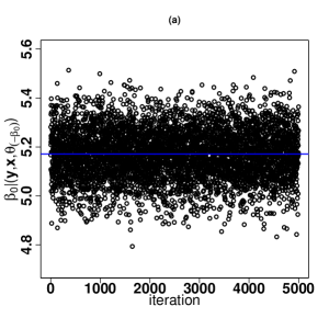
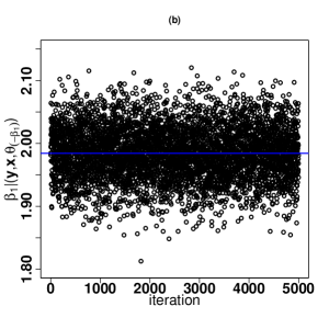
Figure 8.3: Scatterplot of 5000 samples generated from full conditionals: (a) $\beta_{0}\big{|}\bigl{(}\bm{y},\bm{x},\bm{\theta}_{(-\beta_{0})}\bigr{)}$ , (b): $\beta_{1}\big{|}\bigl{(}\bm{y},\bm{x},\bm{\theta}_{(-\beta_{1})}\bigr{)}$, and (c): $\sigma\big{|}\bigl{(}\bm{y},\bm{x},\bm{\theta}_{(-\sigma)}\bigr{)}$. The blue line, in each subfigure, shows the Bayesian estimator.

Example 21 Suppose response variable $Y$ depends linearly on independent variable (covariate) $X$ through a simple linear model as

$$y_{i}= \beta_{0}+\beta_{1}x_{i1}+\beta_{2}x_{i2}+\cdots+\beta_{K}x_{iK}+\epsilon_{i}$$

$$= \bm{x}_{i}^{\top}\bm{\beta}+\epsilon_{i};\leavevmode\nobreak\ \leavevmode\nobreak\ i=1,2,3,\cdots,n,$$

where $\bm{x}_{i}=\bigl{(}1,x_{i1},\cdots,x_{iK}\bigr{)}^{\top}$, $\bm{\beta}=\bigl{(}\beta_{0},\beta_{1},\cdots,\beta_{K}\bigr{)}^{\top}$ is the vector of unknown regression coefficients, and $\epsilon_{i}$s are the model’s theoretical error assumed to follow ${\cal{N}}\bigl{(}0,\sigma^{2}\bigr{)}$ independently (that is, ${\text{cov}}\bigl{(}\epsilon_{i},\epsilon_{j}\bigr{)}=0$ for $i\neq j=1,2,3,\cdots,n$). Of course the skewed Student’s $t$ (Teimouri et al., 2020) and $\alpha$-stable (Nolan and Ojeda-Revah, 2013) may be reasonable candidates for distribution of theoretical error in presence of outliers that yield more robust estimation of ${\bm{\beta}}$ than the Gaussian one. It is known that the least-square (LS) estimator $\hat{\bm{\beta}}_{ls}$ and ML estimator $\hat{\bm{\beta}}_{ml}$, of the regression coefficients $\bm{\beta}$ are the same and given by

$$\hat{\bm{\beta}}_{ML}=\hat{\bm{\beta}}_{LS}=\bigl{(}\bm{X}^{\top}\bm{X}\bigr{)}^{-1}\bm{X}^{\top}\bm{y},$$ (8.23)

where $\bm{y}$ (vector of responses) and $\bm{X}$ is $n\times(K+1)$ design matrix are

$$\bm{y}=\left[\begin{matrix}y_{1}\\ y_{2}\\ \vdots\\ y_{n}\end{matrix}\right],\leavevmode\nobreak\ \bm{X}=\left[\begin{matrix}\bm{x}_{1}\\ \bm{x}_{2}\\ \vdots\\ \bm{x}_{n}\end{matrix}\right]=\left[\begin{matrix}1&x_{11}&x_{12}&\cdots&x_{1K}\\ 1&x_{21}&x_{22}&\cdots&x_{2K}\\ \vdots&\vdots&\vdots&\vdots&\vdots\\ 1&x_{n1}&x_{n2}&\cdots&x_{nK}\\ \end{matrix}\right].$$ (8.24)

Although it is possible to consider a Gaussian conjugate prior for each regression coefficient separately, but we prefer to consider a $(K+1)$-dimensional Gaussian prior for vector of regression coefficients $\bm{\beta}$ and a mutually independent inverse gamma conjugate prior for $\delta=\sigma^{2}$ as

$$\pi(\bm{\beta})= {\cal{N}}_{K+1}\bigl{(}\bm{\beta}\big{|}\bm{\mu}_{0},\Sigma_{0}\bigr{)},$$

$$\pi(\delta)= {\cal{IG}}\Bigl{(}\delta\Big{|}\frac{a_{0}}{2},\frac{b_{0}}{2}\Bigr{)}.$$ (8.25)

It follows that

$$\pi(\bm{\Psi}|\bm{y},\bm{x})= L\bigl{(}\bm{\Psi}\big{|}\bm{y},\bm{x}\bigr{)}\pi(\bm{\beta})$$

$$\propto \delta^{-\frac{n}{2}}\exp\Bigl{\{}-\frac{1}{2\delta}\sum_{i=1}^{n}\bigl{(}y_{i}-\bm{x}_{i}^{\top}\bm{\beta}\bigr{)}^{2}\Bigr{\}}\exp\Bigl{\{}-\frac{1}{2}\bigl{(}\bm{\beta}-\bm{\mu}_{0}\bigr{)}^{\top}\Sigma_{0}^{-1}\bigl{(}\bm{\beta}-\bm{\mu}_{0}\bigr{)}\Bigr{\}}$$

$$\times\Bigl{(}\frac{a_{0}}{2}\Bigr{)}^{\frac{a_{0}}{2}}\frac{\delta^{-a_{0}/2-1}}{\Gamma\bigl{(}\frac{a_{0}}{2}\bigr{)}}\exp\Bigl{\{}-\frac{a_{0}}{2\delta}\Bigr{\}},$$ (8.26)

where $\bm{\Psi}=(\bm{\beta}^{\top},\delta)^{\top}$. For computing the full conditional $\bm{\beta}\big{|}\bigl{(}\bm{y},\bm{x},\bm{\Psi}_{(-\bm{\beta})}\bigr{)}$, it is worth taking into account to the fact that

$$\sum_{i=1}^{n}\bigl{(}y_{i}-\bm{x}_{i}^{\top}\bm{\beta}\bigr{)}^{2}=\sum_{i=1}^{n}y^{2}_{i}-2\bm{\beta}^{\top}\bm{X}^{\top}\bm{y}+\bm{\beta}^{\top}\bm{X}^{\top}\bm{X}\bm{\beta}.$$

Then more algebra shows

$$\pi\bigl{(}\bm{\beta}\big{|}\bm{y},\bm{x},\bm{\Psi}_{(-\bm{\beta})}\bigr{)}\propto \exp\Bigl{\{}-\frac{1}{2}\bigl{(}\bm{\beta}-\bm{\mu}_{\bullet}\bigr{)}^{\top}\Sigma^{-1}_{\bullet}\bigl{(}\bm{\beta}-\bm{\mu}_{\bullet}\bigr{)}\Bigr{\}},$$

where $\bm{\mu}_{\bullet}=\Sigma_{\bullet}\bigl{[}\Sigma_{0}^{-1}\bm{\mu}_{0}+\bm{X}^{\top}\bm{y}\bigr{]}$ and $\Sigma_{\bullet}=\bigl{[}\Sigma_{0}^{-1}+\bm{X}^{\top}\bm{X}\bigr{]}^{-1}$. So,

$$\pi\bigl{(}\bm{\beta}\big{|}\bm{y},\bm{x},\bm{\Psi}_{(-\bm{\beta})}\bigr{)}={\cal{N}}_{K+1}\biggl{(}\bm{\beta}\Big{|}\Sigma_{\bullet}\Bigl{[}\Sigma_{0}^{-1}\bm{\mu}_{0}+\bm{X}^{\top}\bm{y}\Bigr{]},\Sigma_{\bullet}\biggr{)}.$$

Furthermore, it can be seen easily that

$$\pi\bigl{(}{\delta}\big{|}\bm{y},\bm{x},\bm{\Psi}_{(-{\delta})}\bigr{)}={\cal{IG}}\biggl{(}\delta\bigg{|}\frac{a_{0}+n}{2},\frac{b_{0}+\sum_{i=1}^{n}\bigl{(}y_{i}-\bm{x}_{i}^{\top}\bm{\beta}\bigr{)}^{2}}{2}\biggr{]}\biggr{)}.$$

The hyperparameters $a_{0}$ and $b_{0}$ can be estimated in the same way as in Example 8.2, $\bm{\mu}_{0}$ is assumed to be (8.23), and $\Sigma_{0}=\text{cov}\bigl{(}\hat{\bm{\beta}}_{ML}\bigr{)}=\sigma^{2}\bigl{(}\bm{X}^{\top}\bm{X}\bigr{)}^{-1}$. In what follows, we give the steps for computing Bayesian estimation of ${\bm{\Psi}}$ in Example 8.2.

1. Read $N,M$, and determine hyperparameters $a_{0}$, $b_{0}$, $\bm{\mu}_{0}$, and $\Sigma_{0}$;

2. Set $t=0$;

3. Simulate $\bm{\beta}^{(t+1)}$ from the full conditional $\bm{\beta}\big{|}\bigl{(}{\bm{y}},{\bm{x}},\bm{\Psi}_{(-\bm{\beta})}\bigr{)}$ with PDF

   $$\pi\bigl{(}\bm{\beta}\big{|}\bm{y},\bm{x},\bm{\Psi}_{(-\bm{\beta})}\bigr{)}={\cal{N}}_{K+1}\Bigl{(}\bm{\beta}\Big{|}\bm{\mu}_{\bullet},\Sigma_{\bullet}\Bigl{)},$$

   where $\bm{\mu}_{\bullet}=\Sigma_{\bullet}\bigl{[}\Sigma_{0}^{-1}\bm{\mu}_{0}+\bm{X}^{\top}\bm{y}\bigr{]}$ and $\Sigma_{\bullet}=\bigl{[}\Sigma_{0}^{-1}+\bm{X}^{\top}\bm{X}\bigr{]}^{-1}$. So,

4. Having $\bm{\beta}^{(t+1)}$, set ${\delta}^{(t+1)}=\sqrt{z}$ where $z$ follows ${\cal{IG}}$ distribution with PDF

   $${\cal{IG}}\biggl{(}z\bigg{|}\frac{a_{0}+n}{2},\frac{a_{0}+\sum_{i=1}^{n}\bigl{(}y_{i}-\bm{x}_{i}^{\top}\bm{\beta}^{(t+1)}\bigr{)}^{2}}{2}\biggr{]}\biggr{)}.$$

5. If $t=N$, then go to the next step. Otherwise set $t+1\rightarrow t$ and return to step 3;

6. The average of sequence $\bigl{\{}\bm{\Psi}^{(M+1)},\bm{\Psi}^{(M+2)},\cdots,\bm{\Psi}^{(M+N)}\bigr{\}}$ sampled from target distribution with PDF $\pi\bigl{(}\bm{\Psi}|\bm{y},\bm{x}\bigr{)}$ is the Bayesian estimator $\hat{\bm{\Psi}}_{B}=\bigl{(}\hat{\bm{\beta}}_{B},\hat{\sigma}_{B}\bigr{)}^{\top}$.

Herein, Example 8.2 will be illustrated with computing the Bayesian estimator of regression plane coefficients fitted to trees data. This data set is available in R environment. The corresponding R code for implementing this example is given as follows. The output of the Gibbs sampler is displayed in Figure 8.4.

⬇

1R> set.seed(20240601)

2R> data(trees)

3R> y <- trees$Volume;

4R> n <- length(y)

5R> x <- cbind(trees$Girth, trees$Height)

6R> K <- 3 # number of regression coefficients

7R> X <- as.matrix( cbind(1, x), nrow = n, ncol = K)

8R> out <- lm(y ~ X[, 2] + X[, 3])

9R> ML <- as.vector( coefficients(out) )

10R> error <- as.vector(y - X%*%ML)

11R> param0 <- var(error)

12R> obj <- function(par) -sum( -log(par[2])/2 + lgamma( (par[1]+1)/2 ) -

13+ lgamma( par[1]/2 ) - (par[1]+1)/2*log( 1 + error^2/par[2] ))

14R> theta0 <- optim( rep(param0, 2), fn = obj, method = "L-BFGS-B",

15+ lower = rep(0.5, 2), upper = rep(n, 2) )$par

16R> N <- 5000 # number of generations

17R> M <- 2000 # size of burn-in period

18R> Psi <- matrix(0, nrow = N, ncol = K + 1)

19R> delta <- 1

20R> Psi[1, ] <- c(ML, delta )

21R> hat <- Psi[1, ]

22R> Mu0 <- ML

23R> sigma2_hat <- theta0[2]/abs(theta0[1] - 1)

24R> Sigma0_inv <- solve( sigma2_hat*solve(t(X)%*%X) )

25R> j <- 1

26R> while(j < N)

27+ {

28+ Sigma_bullet <- solve( Sigma0_inv + t(X)%*%X )

29+ Mu_bullet <- Sigma_bullet%*%( Sigma0_inv%*%Mu0 + t(X)%*%y )

30+ Psi[j+1, 1:K] <- mvrnorm(1, mu = Mu_bullet, Sigma = Sigma_bullet )

31+ error <- as.vector( y - X%*%Psi[j+1, 1:K] )

32+ SSE <- sum(error^2)

33+ delta <- 1/sqrt(rgamma( 1, shape = (theta0[1] + n)/2,

34+ rate = (theta0[2] + SSE)/2 ) )

35+ Psi[j + 1, 4] <- delta

36+ j <- j + 1

37+ }

38R> Bayes <- apply(Psi[(N - M + 1):N, ], 2, mean)

39R> list(beta0=Bayes[1],beta1=Bayes[2],beta2=Bayes[3],sigma=sqrt(Bayes[4]))

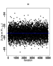
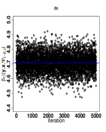
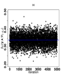
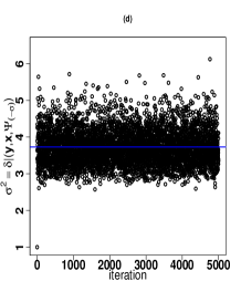
Figure 8.4: Scatterplot of 5000 samples generated from full conditionals: (a) $\beta_{0}\big{|}\bigl{(}\bm{y},\bm{x},\bm{\Psi}_{(-\beta_{0})}\bigr{)}$ , (b): $\beta_{1}\big{|}\bigl{(}\bm{y},\bm{x},\bm{\Psi}_{(-\beta_{1})}\bigr{)}$, (c): $\beta_{2}\big{|}\bigl{(}\bm{y},\bm{x},\bm{\Psi}_{(-\beta_{2})}\bigr{)}$, and (d): $\sigma^{2}=\delta\big{|}\bigl{(}\bm{y},\bm{x},\bm{\Psi}_{(-\delta)}\bigr{)}$. The blue line, in each subfigure, shows the Bayesian estimator.

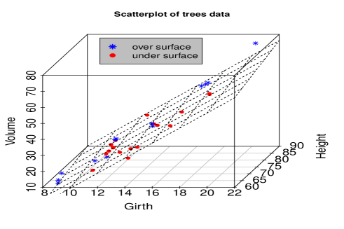
Figure 8.5: Scatterplot of trees data. Superimposed is the fitted regression plane whose coefficients are estimated through the Bayesian paradigm.

8.3 Gibbs sampling in Bayesian paradigm with one latent variable

Sometimes implementing the MCMC techniques such as MH or Gibbs sampling for drawing the Bayesian inference is computationally inefficient due to the complex form of the posterior. In such cases, inference about the unknown parameter(s) may be drawn by involving some latent (unobservable or augmented) variable(s). The rationale behind using the term “latent” traced back to this fact that the experimenter cannot observe some extra variable(s) existing in the model at quick glance, but there exists. For example, let random vector $\bm{X}=(X_{1},\cdots,X_{p})^{\top}$ follows a $p$-dimensional Student’s $t$ distribution with $\nu>0$ degrees of freedom with PDF given by (5.56). Evidently implementing the MH or Gibbs sampling in which the full conditionals are constructed based on PDF (5.56) is quite difficult. On the other hand, it is easy to see that $\bm{X}$ admits the stochastic representation $\bm{X}\mathop{=}\limits^{d}\bm{\mu}+\Sigma^{1/2}\bm{Z}/\sqrt{G}$ where $\bm{Z}\sim{\cal{N}}_{p}\bigl{(}\bm{0}_{p},\bm{I}_{p}\bigr{)}$ and $G\sim{\cal{G}}(\nu/2,\nu/2)$ (${\cal{G}}(a,b)$ accounts for a gamma distribution with shape and rate parameters, $a$ and $b$, respectively.). Herein, random variable $G$ plays the role of a latent variable. We also can consider more than one latent variable in each statistical model. Nevertheless, the Gibbs sampling is a very useful approach in presence of latent variable in the case of either sampling or Bayesian inference. In what follows, we give a definition that plays a main role in understanding Bayesian inference for the parameters of a statistical model that includes latent variable(s).

Definition 8.3.1.

Let $x_{1},\cdots,x_{n}$ are a sample of $n$ independent observed values from a model with PDF $f(x|\bm{\theta})$ where $\bm{\theta}$ is the unknown parameter vector. If model includes latent variable $g$ whose PDF is $f(g|\bm{\theta}_{g})$ in which $\bm{\theta}_{g}$ is the unknown parameter vector of distribution of $g$. Furthermore, let $f(x,g|\bm{\Psi})$ is the joint PDF of vector $(x,g)^{\top}$ where $\bm{\Psi}=\bm{\theta}\cup\bm{\theta}_{g}$. Then we have:

• The sequence $\bigl{\{}x_{1},\cdots,x_{n}\bigr{\}}$ and $\bigl{\{}g_{1},\cdots,g_{n}\bigr{\}}$, are called the observed and latent data, respectively.

• The sequence of paired-data $\{\bigl{(}x_{1},g_{1}\bigr{)},\cdots,\bigl{(}x_{n},g_{n}\bigr{)}\}$ is called complete data that evidently is the union of observed and latent data.

• The complete data likelihood function becomes

  $$L_{c}(\bm{\Psi}|\bm{x},\bm{g})=f(\bm{x},\bm{g}|\bm{\Psi})=\prod_{i=1}^{n}f\bigl{(}x_{i}\big{|}g_{i},\bm{\Psi}\bigr{)}=\prod_{i=1}^{n}f\bigl{(}x_{i}\big{|}g_{i},\bm{\theta}\bigr{)}f\bigl{(}g_{i}\big{|}\bm{\theta}_{g}\bigr{)}.$$ (8.27)

Definition 8.3.1 is based on just one latent variable, but can be easily extended and is valid for two or more latent variables. It is noteworthy that for a Bayesian paradigm in which we have latent variable(s), we rewrite the posterior (8.2) in terms of the complete data likelihood function as follows.

$$\pi(\bm{\Psi}|\bm{x},\bm{g})\propto L_{c}(\bm{\Psi}|\bm{x},\bm{g})\pi(\bm{\Psi}),$$ (8.28)

where $L_{c}(\bm{\Psi}|\bm{x},\bm{g})$ is given by Definition 8.3.1. To implement the Bayesian paradigm, notice that the conditional PDF $f\bigl{(}x_{i}\big{|}g_{i},\bm{\theta}\bigr{)}$ and marginal PDF $f\bigl{(}g_{i}\big{|}\bm{\theta}_{g}\bigr{)}$ given in RHS of (8.27) must be known and possibly in closed form. In what follows, we give an example in which Bayesian inference on the parameters of a Student’s $t$ distribution is desired.

Example 22 He et al. (2021) Suppose ${\underline{\bm{x}}}=\bigl{(}\bm{x}_{1},\cdots,\bm{x}_{n}\bigr{)}$ is vector of $n$ independent observations from a $p$-dimensional Student’s $t$ distribution. Recall that for each Student’s $t$ random vector $\bm{X}$ we can write $\bm{X}\mathop{=}\limits^{d}\bm{\mu}+\Sigma^{1/2}\bm{Z}/\sqrt{G}$. Evidently $\bm{X}$ admits the hierarchy given by

$$\bm{X}|G \sim f\bigl{(}\bm{x}_{i}|g_{i},\bm{\theta}=(\bm{\mu},\Sigma)\bigr{)}={\cal{N}}_{p}\Bigl{(}\bm{x}_{i}\Big{|}\bm{\mu},\frac{\Sigma}{{G}}\Bigr{)},$$

$$G \sim f\bigl{(}g_{i}\big{|}\bm{\theta}_{g}=\nu\bigr{)}={\cal{G}}\bigl{(}g_{i}\big{|}\nu/2,\nu/2\bigr{)},$$ (8.29)

where ${\cal{N}}_{p}\bigl{(}.\big{|}\bm{\mu},{\Sigma}\bigr{)}$ denotes the PDF of a $p$-dimensional Gaussian distribution with location vector $\bm{\mu}$ and scale matrix ${\Sigma}$ and ${\cal{G}}(\cdot\big{|}a,b)$ accounts for the PDF of a gamma distribution with shape parameter $a$ and rate parameter $b$. Hence, the complete data likelihood is

$$L_{c}(\bm{\Psi}|{\underline{\bm{x}}},\bm{g})= \prod_{i=1}^{n}\Bigl{[}{\cal{N}}_{p}\bigl{(}\bm{x}_{i}\big{|}\bm{\mu},[g_{i}]^{-1}\Sigma\bigr{)}f\bigl{(}g_{i}\big{|}\bm{\theta}_{g}\bigr{)}\Bigr{]}$$

$$= \Bigl{[}\Gamma\Bigl{(}\frac{\nu}{2}\Bigr{)}\Bigr{]}^{-n}\Bigl{(}\frac{\nu}{2}\Bigr{)}^{\frac{n\nu}{2}}$$

$$\times\prod_{i=1}^{n}\biggl{\{}\bigl{[}g_{i}\bigr{]}^{\frac{\nu+p}{2}-1}\exp\Bigl{\{}-\frac{g_{i}}{2}\Bigl{[}\nu+\bigl{(}\bm{x}_{i}-\bm{\mu}\bigr{)}^{\top}\Sigma^{-1}\bigl{(}\bm{x}_{i}-\bm{\mu}\bigr{)}\Bigr{]}\Bigr{\}}\biggr{\}},$$ (8.30)

where $\bm{\Psi}=\bm{\theta}\cup\bm{\theta}_{g}=(\bm{\mu},\Sigma,\nu)$ is the model’s parameter vector. For the prior, we proceed to assume independence, that is $\pi(\bm{\Psi})=\pi(\bm{\mu})\pi(\Sigma)\pi(\nu)$ in which $\pi(\bm{\mu})$ and $\pi(\Sigma)$ are conjugate Gaussian and inverse Wishart priors. Furthermore, we let $\pi(\nu)$ to be the PDF of a gamma distribution. We have

$$\pi(\bm{\mu}) \sim{\cal{N}}_{p}({\cal{M}}_{0},{\cal{S}}_{0}),$$

$$\pi(\Sigma) \sim{\cal{IW}}({\cal{D}}_{0},\nu_{0}),$$

$$\pi(\nu) \sim{\cal{G}}\bigl{(}a_{0},b_{0}\bigr{)}.$$

We note that in above an objective prior such as Jeffreys’ prior can be chosen, however, the most concern is placed on $\pi(\nu)$ that was proposed by Fernández and Steel (1999) to be $\pi(\nu)=10\exp\{-10\nu\}$. It can be seen that the jeffreys’ prior becomes $\pi(\bm{\mu},\Sigma,\nu)=|\Sigma|^{-(p+1)/2}$ (Fernández and Steel, 1999), and so considering a flat prior for both of $\bm{\mu}$ and $\nu$ is acceptable. We note that for drawing inference about $\bm{\Psi}$, one needs to generate from full conditional of the latent variable too. So, by considering $\bm{\mu}$, $\Sigma$, $\nu$, and $g$ (latent variable) as the model’s variables, within a Gibbs sampling framework, we proceed to sample from full conditionals $\bm{\mu}|({\Sigma},\nu)$, $\Sigma|(\bm{\mu},\nu)$, $\nu|(\bm{\mu},{\Sigma})$. But, keep in mind that for each observed data $\bm{y}_{i}$, $g_{i}$ (for $i=1,\cdots,n$) is also latent unobservable). In order to $g_{i}$ being known, we proceed to simulate $g_{i}$ (for $i=1\cdots,n$) for each $\bm{y}_{i}$. To do this, in each iteration of the Gibbs sampling, we simulate (for each $\bm{y}_{i}$) from full conditional $g_{i}\big{|}\bigl{(}\bm{\mu},{\Sigma},\nu,{\bm{y}}_{i}\bigr{)}$ as follows. From RHS of (8.3), for a single observed value $\bm{y}_{i}$, it follows that

$$\pi\bigl{(}g_{i}\big{|}\bm{\Psi},\bm{y}_{i}\bigr{)} \propto\bigl{[}g_{i}\bigr{]}^{\frac{\nu+p}{2}-1}\exp\Bigl{\{}-\frac{g_{i}}{2}\Bigl{[}\nu+\bigl{(}\bm{y}_{i}-\bm{\mu}\bigr{)}^{\top}\Sigma^{-1}\bigl{(}\bm{y}_{i}-\bm{\mu}\bigr{)}\Bigr{]}\Bigr{\}}.$$

This means that

$$\pi\bigl{(}g_{i}\big{|}\bm{\Psi},\bm{y}_{i}\bigr{)}\sim{\cal{G}}\Bigl{(}(\nu+p)/2,\nu/2+\bigl{(}\bm{y}_{i}-\bm{\mu}\bigr{)}^{\top}\Sigma^{-1}\bigl{(}\bm{y}_{i}-\bm{\mu}\bigr{)}/2\Bigr{)}.$$

Let $\bm{\Psi}_{(-\theta)}$ denote the whole parameter vector excluding its element $\theta$, once we have generated a whole vector of latent variable as $\bm{g}=(g_{1},\cdots,g_{n})^{\top}$, the complete data is known and we proceed to simulate from other full conditionals as follows.

• full conditional of $\bm{\mu}\big{|}\bigl{(}{{\underline{\bm{y}}}},\bm{g},\Psi_{(-\bm{\mu})}\bigr{)}$: By considering a conjugate prior, shown earlier by $\pi(\bm{\mu})\sim{\cal{N}}_{p}({\cal{M}}_{0},{\cal{S}}_{0})$, we have

  $$\pi\bigl{(}\bm{\mu}\big{|}{{\underline{\bm{y}}}},\bm{g},\Psi_{(-\bm{\mu})}\bigr{)}\propto L_{c}(\bm{\Psi}|{\underline{\bm{x}}},\bm{g}){\cal{N}}_{p}\bigl{(}\bm{\mu}\big{|}{\cal{M}}_{0},{\cal{S}}_{0}\bigr{)}.$$

  More algebra shows that

  $$\bm{\mu}\big{|}\bigl{(}{{\underline{\bm{y}}}},\bm{g},\Psi_{(-\bm{\mu})}\bigr{)}\sim{\cal{N}}_{p}\Bigl{(}{\cal{Q}}_{0}\Bigl{[}{\cal{S}}^{-1}_{0}{\cal{M}}_{0}+\Sigma^{-1}\sum_{i=1}^{n}g_{i}\bm{y}_{i}\Bigr{]},{\cal{Q}}_{0}\Bigr{)},$$

  where

  $${\cal{Q}}_{0}=\Bigl{[}{\cal{S}}^{-1}_{0}+\Sigma^{-1}\sum_{i=1}^{n}g_{i}\Bigr{]}^{-1}.$$

• full conditional of ${\Sigma}\big{|}\bigl{(}{{\underline{\bm{y}}}},\bm{g},\Psi_{(-{\Sigma})}\bigr{)}$: By considering a conjugate prior, that is ${\Sigma}\sim{\cal{IW}}\bigl{(}{\cal{D}}_{0},\nu_{0}\bigr{)}$, we can write

  $$\pi\bigl{(}\Sigma\big{|}{{\underline{\bm{y}}}},\bm{g},\Psi_{(-\Sigma)}\bigr{)}\propto L_{c}(\bm{\Psi}|{\underline{\bm{x}}},\bm{g}){\cal{IW}}(\Sigma\big{|}{\cal{D}}_{0},\nu_{0}\bigr{)},$$

  where ${\cal{IW}}(\Sigma\big{|}{\cal{D}}_{0},\nu_{0}\bigr{)}$ denotes the PDF of an inverse Wishart distribution. More algebra shows that

  $${\Sigma}\big{|}\bigl{(}{{\underline{\bm{y}}}},\bm{g},\Psi_{(-{\Sigma})}\bigr{)}\sim{\cal{IW}}\bigl{(}{\cal{R}}_{0},\nu_{0}+n\bigr{)},$$

  where ${\cal{R}}_{0}={\cal{D}}_{0}+\sum_{i=1}^{n}g_{i}\bigl{(}\bm{y}_{i}-\bm{\mu}\bigr{)}\bigl{(}\bm{y}_{i}-\bm{\mu}\bigr{)}^{\top}$.

• full conditional of ${\nu}\big{|}\bigl{(}{\underline{\bm{y}}},\bm{g},\Psi_{(-{\nu})}\bigr{)}$: By considering a truncated exponential distribution with PDF $\pi(\nu)={\cal{G}}\bigl{(}\nu-2\big{|}1,b_{0}\bigr{)}$ for $\nu\geq 2$, we can write

  $$\pi\bigl{(}\nu\big{|}{\underline{\bm{y}}},\bm{g},\Psi_{(-{\nu})}\bigr{)} \propto L_{c}(\bm{\Psi}|\underline{\bm{x}},\bm{g})\pi(\nu)$$

  $$\propto\Bigl{[}\Gamma\Bigl{(}\frac{\nu}{2}\Bigr{)}\Bigr{]}^{-n}\Bigl{(}\frac{\nu}{2}\Bigr{)}^{\frac{n\nu}{2}}b_{0}\exp\Bigl{\{}-\frac{\nu}{2}\bigl{[}2b_{0}+\sum_{i=1}^{n}g_{i}\bigr{]}\Bigr{\}}\prod_{i=1}^{n}\bigl{[}g_{i}\bigr{]}^{\frac{\nu}{2}}.$$ (8.31)

  As it is seen, the full conditional (• ‣ 8.3) has not closed form. The MH algorithm can be suggested to draw sample from this full conditional. It is easy to check that $\pi\bigl{(}\nu\big{|}{\underline{\bm{y}}},\bm{g},\Psi_{(-{\nu})}\bigr{)}$ is log-concave and hence the ARS-within-Gibbs sampling algorithm can be suggested for simulating from this full conditional. For computing the vector of hyperparameter $\bm{\theta}_{0}=b_{0}$, it follows from hierarchy (8.3) that

  $$m\bigl{(}\underline{\bm{x}}|{b}_{0}\bigr{)} =\Pi_{i=1}^{n}\int_{2}^{\infty}f\bigl{(}\bm{x}_{i}\big{|}\nu\bigr{)}\pi\bigl{(}\nu\big{|}{b}_{0}\bigr{)}d\nu$$

  $$=\Pi_{i=1}^{n}\int_{2}^{\infty}\frac{\Gamma\bigl{(}\frac{\nu+p}{2}\bigr{)}\pi\bigl{(}\nu\big{|}{b}_{0}\bigr{)}d\nu}{(\nu\pi)^{\frac{p}{2}}\Gamma\bigl{(}\frac{\nu}{2}\bigr{)}|\Sigma|^{\frac{1}{2}}\bigl{[}1+\frac{(\bm{x}-\bm{\mu})^{\top}\Sigma^{-1}(\bm{x}-\bm{\mu})}{\nu}\bigr{]}^{\frac{\nu+p}{2}}},$$ (8.32)

  where $\underline{\bm{x}}=(\bm{x}_{1},\cdots,\bm{x}_{n})$. Maximizing the RHS of (• ‣ 8.3) with respect to $b_{0}$ is not a simple task, an so we proceed to compute the moment-type estimator of $b_{0}$ as follows. First notice that

  $$E\bigl{[}(\bm{X}-\bm{\mu})(\bm{X}-\bm{\mu})^{\top}\big{|}b_{0}\bigr{)}= \int_{2}^{\infty}\int_{\mathbb{R}^{p}}(\bm{x}-\bm{\mu})(\bm{x}-\bm{\mu})^{\top}f\bigl{(}\bm{x}\big{|}\nu\bigr{)}\pi\bigl{(}\nu\big{|}{b}_{0}\bigr{)}d\bm{x}d\nu$$

  $$= \int_{2}^{\infty}\int_{\mathbb{R}^{p}}\frac{(\bm{x}-\bm{\mu})(\bm{x}-\bm{\mu})^{\top}\Gamma\bigl{(}\frac{\nu+p}{2}\bigr{)}}{(\nu\pi)^{\frac{p}{2}}\Gamma\bigl{(}\frac{\nu}{2}\bigr{)}|\Sigma|^{\frac{1}{2}}\bigl{[}1+\frac{(\bm{x}-\bm{\mu})^{\top}\Sigma^{-1}(\bm{x}-\bm{\mu})}{\nu}\bigr{]}^{\frac{\nu+p}{2}}}$$

  $$\times\frac{b^{b_{0}-1}_{0}}{\Gamma(b_{0})}(\nu-2)^{b_{0}-1}\exp\{-b_{0}(\nu-2)\}d\bm{x}d\nu$$

  $$= \int_{2}^{\infty}\Bigl{(}\frac{\nu}{\nu-2}{\Sigma}\Bigr{)}\frac{b^{b_{0}-1}_{0}}{\Gamma(b_{0})}(\nu-2)^{b_{0}-1}\exp\{-b_{0}(\nu-2)\}d\nu$$

  $$= 3-\frac{1}{b_{0}}.$$

  Let AD denote the average of diagonal elements of matrix $\big{[}\sum_{i=1}^{n}(\bm{x}^{2}_{i}-\bm{\mu})(\bm{x}^{2}_{i}-\bm{\mu})^{\top}/n\bigr{]}\Sigma^{-1}$, then $b_{0}$ can be exploited as $b_{0}=1/(3-AD)$.

Furthermore, one can employ the MH-within-Gibbs sampling technique for drawing sample from full conditional (• ‣ 8.3). To this end, we assume gamma distribution for the prior with PDF $\pi(\nu)={\cal{G}}\bigl{(}.\big{|}b_{0},b_{0}\bigr{)}$. Herein there is just one hyperparameter that we prefer to compute it as $b_{0}=1/(3-AD)$. We further choose $gamma\bigl{(}b_{0},b_{0}\bigr{)}$ as the candidate. For other hyperparameters including ${\cal{M}}_{0},{\cal{S}}_{0},{\cal{D}}_{0}$, and $\nu_{0}$, in example above, we set ${\cal{M}}_{0}$ to be the mean of ${\underline{\bm{y}}}$ and $\nu_{0}=1$. For ${\cal{S}}_{0}$ and ${\cal{D}}_{0}$ we suggest to consider $\bm{I}_{p}$. The steps for computing the Bayesian estimator of ${\bm{\Psi}}$ are given by Algorithm 6.

Algorithm 6 Bayesian inference for Student’s $t$ distribution

1:Read $N$, $M$, ${{K}}$, ${\cal{M}}_{0}$, ${\cal{S}}_{0}$, ${\cal{D}}_{0}$, and $\nu_{0}$;

2:Set $t\leftarrow 0$;

3:Set $\bm{\mu}^{(0)}\leftarrow{\cal{M}}_{0}$, $\Sigma^{(0)}\leftarrow 1/n\sum_{i=1}^{n}\bigl{(}\bm{y}_{i}-\bm{\mu}^{(0)}\bigr{)}\bigl{(}\bm{y}_{i}-\bm{\mu}^{(0)}\bigr{)}^{\top}$, ${\nu}^{(0)}=2$,

4:and set $\bm{\Psi}^{(0)}=\bigl{(}\bm{\mu}^{(0)},\Sigma^{(0)},\nu^{(0)}\bigr{)}$;

5:while $t\leq N$ do

6:     Set $i=1$;

7:     while $i\leq n$ do

8:         Simulate $g_{i}$ from ${\cal{G}}(a,b)$ where $a=(\nu^{(t)}+p+1)/2$ and $b=$

9:         $\Bigl{[}\nu^{(t)}/2+\bigl{(}\bm{y}_{i}-\bm{\mu}^{(t)}\bigr{)}^{\top}\bigl{[}\Sigma^{(t)}\bigr{]}^{-1}\bigl{(}\bm{y}_{i}-\bm{\mu}^{(t)}\bigr{)}\Bigr{]}/2$;

10:         Set $i\leftarrow i+1$;      

11:     end

12:     Generate $\bm{\mu}^{(t+1)}$ from ${\cal{N}}_{p}\Bigl{(}{\cal{Q}}_{0}\Bigl{[}{\cal{S}}^{-1}_{0}{\cal{M}}_{0}+\bigl{[}\Sigma^{(t)}\bigr{]}^{-1}\sum_{i=1}^{n}g_{i}\bm{y}_{i}\Bigr{]},{\cal{Q}}_{0}\Bigr{)}$ where

13:     ${\cal{Q}}_{0}=\Bigl{[}{\cal{S}}^{-1}_{0}+\bigl{[}\Sigma^{(t)}\bigr{]}^{-1}\sum_{i=1}^{n}g_{i}\Bigr{]}^{-1}$;

14:     Generate $\Sigma^{(t+1)}$ from ${\cal{IW}}\bigl{(}{\cal{R}}_{0},\nu_{0}+n\bigr{)}$ where ${\cal{R}}_{0}={\cal{D}}_{0}$ +

15:     $\sum_{i=1}^{n}g_{i}\bigl{(}\bm{y}_{i}-\bm{\mu}^{(t+1)}\bigr{)}\bigl{(}\bm{y}_{i}-\bm{\mu}^{(t+1)}\bigr{)}^{\top}$;

16:     Use the MH-within-Gibbs sampling technique for simulating $\nu^{(t+1)}$

17:     as follows;

18:     Set $k=0$ and $x_{0}\leftarrow\nu_{0}$

19:     while $k\leq{{K}}$ do

20:         $x_{0}\sim{\cal{G}}\bigl{(}a_{0},b_{0}\bigr{)}$;

21:         Generate $x^{(k+1)}\sim{\cal{G}}\bigl{(}a_{0},b_{0}\bigr{)}$;

22:         Compute $p\bigl{(}x^{(k)}\rightarrow x^{(k+1)}\bigr{)}=\min\bigl{\{}1,\exp\{R_{1}-R_{2}\}\bigr{\}}$ where

23:         $R_{1}=-n\log\Gamma\bigl{(}\frac{x^{(k+1)}}{2}\bigr{)}+\frac{nx^{(k+1)}}{2}\log\bigl{(}\frac{x^{(k+1)}}{2}\bigr{)}+(b_{0}-1)\log x^{(k+1)}$

24:         $-\frac{x^{(k+1)}}{2}\bigl{[}2b_{0}+\sum_{i=1}^{n}g_{i}\bigr{]}+\frac{x^{(k+1)}}{2}\sum_{i=1}^{n}\log g_{i}$

25:         and

26:         $R_{2}=-n\log\Gamma\bigl{(}\frac{x^{(k)}}{2}\bigr{)}+\frac{nx^{(k)}}{2}\log\bigl{(}\frac{x^{(k)}}{2}\bigr{)}+(b_{0}-1)\log x^{(k)}$

27:         $-\frac{x^{(k)}}{2}\bigl{[}2b_{0}+\sum_{i=1}^{n}g_{i}\bigr{]}+\frac{x^{(k)}}{2}\sum_{i=1}^{n}\log g_{i}$;

28:         Generate $u\sim{\cal{U}}(0,1)$;

29:         If $u<p\bigl{(}x^{(k)},x^{(k+1)}\bigr{)}$ then $x^{(k)}\rightarrow x^{(k+1)}$ and $k\rightarrow k+1$;

30:         Repeat algorithm from line (21);

31:         If $k={{K}}$ then $\nu^{(t+1)}\leftarrow x^{(k+1)}$ and stop the algorithm;      

32:     end

33:Set $\bm{\Psi}^{(t+1)}\leftarrow\bigl{(}\bm{\mu}^{(t+1)},\Sigma^{(t+1)},\nu^{(t+1)}\bigr{)}$ and $t\leftarrow t+1$;

34:end

35:Sequence $\bigl{\{}\bm{\Psi}^{(M)},\bm{\Psi}^{(M+1)},\cdots,\bm{\Psi}^{(M)}\bigr{\}}$ is a sample of size $N-M+1$ from

36:posterior with PDF $\pi\bigl{(}\bm{\Psi}|\underline{\bm{x}})$;

37:The Bayesian estimator of $\hat{\bm{\Psi}}_{B}$ is given by $\frac{1}{N-M+1}\sum_{t=1}^{N-M+1}\bm{\Psi}^{(t)}$.

The pertaining R code for implementing example above is given as follows. The R code is applied to a sample of $n=500$ realizations have been generated from a bivariate Student’s $t$ distribution with parameters $\bm{\mu}=(0,2)^{\top}$, $\sigma_{11}=1$, $\sigma_{12}=-0.50$, $\sigma_{22}=0.75$, and $\nu=5$. The output of the Gibbs sampler is displayed in Figure 8.6.

⬇

1R > rssg<-function(n, nu, Mu, Sigma)

2+ {

3+ Dim <- length(Mu)

4+ Y <- matrix(NA, nrow = n, ncol = Dim)

5+ for (i in 1:n)

6+ {

7+ Z <- rgamma(1, shape = nu/2, rate = nu/2)

8+ X <- mvrnorm(n = 1, mu = rep(0, Dim), Sigma = Sigma )

9+ Y[i, ] <- Mu + X/sqrt(Z)

10+ }

11+ Y

12+ }

13R > f.a <- function(x, b0, y)

14+ {

15+ n <- length(y)

16+ -n*lgamma(x/2) + n*(x/2)*log(x/2) - x/2*( 2*b0 + sum(y) ) + x/2*sum( log(y) ) + (b0-1)*log(x)

17+ }

18R > fprim.a <- function(x, b0, y)

19+ {

20+ n <- length(y)

21+ -n*digamma(x/2)/2 + n/2 + n/2*log(x/2) - ( 2*b0 + sum(y) )/2 + sum( log(y) )/2 + (b0-1)/x

22+ }

23R > set.seed(20240529)

24R > library(MASS); library(ars)

25R > n <- 500; nu <- 5; Mu <- c(0, 2)

26R > Sigma <- matrix( c(1,-0.5,-0.5,0.75), 2, 2)

27R > Y <- rssg(n, nu, Mu, Sigma)

28R > N <- 5000; M <- 2000; p <- length(Mu)

29R > Psi <- matrix(0, nrow = N, ncol = p + 1 + p^2)

30R > g <- rate <- rep(0, n)

31R > S0Mu <- diag(2); M0Mu <- rep(0, 2); nu0 <- 2

32R > D0 <- matrix(diag(2), 2, 2)

33R > for(j in 1:N)

34+ {

35+ rate <- mahalanobis(x = Y, center = Mu, cov = Sigma )

36+ for(i in 1:n) g[i] <- rgamma( 1, shape = (nu + p)/2, rate = rate[i]/2 + nu/2 )

37+ Sigmainv <- solve( Sigma )

38+ dy <- mahalanobis( Y, center = Mu, cov = Sigma )

39+ Sum.g <- sum(g)

40+ M_sum <- rowSums( sapply(1:n, function(i) g[i]*c( Y[i, ] ) ) )

41+ Q <- solve( solve( S0Mu ) + Sigmainv*Sum.g )

42+ Mu <- c( mvrnorm(1, mu = Q%*%( solve( S0Mu )%*%M0Mu +

43+ Sigmainv%*%M_sum ) , Sigma = Q) )

44+ Psi[j, 1:p] <- Mu

45+ R0 <- matrix(0, nrow = p, ncol = p)

46+ for(i in 1:n){R0 <- R0 + g[i]*c( Y[i, ] - Mu )%*%t(c( Y[i, ] - Mu ))}

47+ Sigma <- solve(rWishart(1, df = nu0 + n, Sigma = solve(D0 + R0) )[,,1])

48+ Psi[j, (p+1):(p + p^2)] <- as.numeric(Sigma)

49+ b0 <- 1/(3-(cov(Y)%*%solve(Sigma))[1,1])

50+ nu <- ars(1, f.a, fprim.a, x = c(2, 5, 10, 50), m = 4,

51+ lb = TRUE, xlb = 2, b0 = b0, y = g)

52+ Psi[j, p + 1 + p^2] <- nu

53+ }

54R > Psi.hat <- apply(Psi[(N - M + 1):N, ], 2, mean)

55R > Mu <- Psi.hat[1:p]

56R > Sigma <- Psi.hat[(p+1):(p + p^2)]

57R > nu <- Psi.hat[p + 1 + p^2]

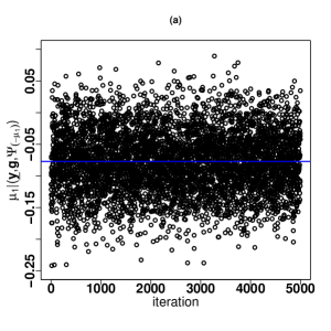
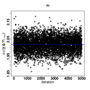
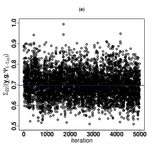
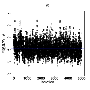
Figure 8.6: Scatterplot of 5000 samples generated from full conditionals: (a) $\mu_{1}\big{|}\bigl{(}{{\bm{y}}},{\bm{g}},\Psi_{(-{\mu}_{1})}\bigr{)}$, (b): ${\mu}_{2}\big{|}\bigl{(}{{\bm{y}}},{\bm{g}},\Psi_{(-{\mu}_{2})}\bigr{)}$, (c): ${\Sigma}_{11}\big{|}\bigl{(}{{\bm{y}}},{\bm{g}},\Psi_{(-\Sigma_{11})}\bigr{)}$, (d) ${\Sigma}_{12}\big{|}\bigl{(}{{\bm{y}}},{\bm{g}},\Psi_{(-\Sigma_{12})}\bigr{)}$, (e) ${\Sigma}_{22}\big{|}\bigl{(}{{\bm{y}}},{\bm{g}},\Psi_{(-\Sigma_{22})}\bigr{)}$, and (f) ${\nu}\big{|}\bigl{(}{{\bm{y}}},{\bm{g}},\Psi_{(-\nu)}\bigr{)}$. The blue line, in each subfigure, shows the Bayesian estimator.

8.4 Gibbs sampling in Bayesian paradigm with two latent variables

8.4.1 Heavy-tailed skew models

The Bayesian paradigm for $\text{SG}_{p,q}(\bm{\mu},\Sigma,{\Lambda})$ distribution with representation (6.24) has been developed by Liseo and Parisi (2013). The skew Gaussian model introduced in Section 6.2 can be developed for modelling the heavy tailed skewed data. This can be accomplished by involving an extra latent variable $G$. Let

$$\bm{Y}\mathop{=}\limits^{d}\bm{\mu}+\frac{\bm{X}}{\sqrt{h(G)}},$$ (8.33)

in which $\bm{X}\sim\text{SG}_{p,q}(\bm{0}_{p},\Sigma,{\Lambda})$ and $h(\cdot)$ is a continuous monotone real function. Equivalently,

$$\bm{Y}\mathop{=}\limits^{d}\bm{\mu}+\frac{{\Lambda}\big{|}\bm{Z}_{0}\big{|}}{\sqrt{h(G)}}+{\Sigma}^{\frac{1}{2}}\frac{\bm{Z}_{1}}{\sqrt{h(G)}}.$$ (8.34)

It is easy to see that random vector $\bm{Y}$ in (8.34) admits the hierarchy given by

$$\bm{Y}|{\bm{U}},G \sim{\cal{N}}_{p}\Bigl{(}\bm{\mu}+{\Lambda}{\bm{U}},\frac{\Sigma}{h(G)}\Bigr{)},$$

$${\bm{U}}|G \sim{\cal{HN}}_{q}\Bigl{(}\bm{0}_{q},\frac{\bm{I}_{q}}{h(G)}\Bigr{)},$$

$$G \sim f(g|\bm{\theta}),$$ (8.35)

where the short form ${\cal{HN}}_{q}(\bm{0}_{q},\Sigma)$ accounts for the half-normal distribution truncated on ${{\mathbb{R}}}^{q+}$ with a zero-location vector of length $q$ and scale matrix $\Sigma$. Regarding $\bigl{\{}\bm{y}_{1},\cdots,\bm{y}_{n}\bigr{\}}$ as the sequence of observed data and two sequences of latent variables are represented as $\bigl{\{}\bm{u}_{1},\cdots,\bm{u}_{n}\bigr{\}}$ and $\bigl{\{}g_{1},\cdots,g_{n}\bigr{\}}$. Based on hierarchy (8.4.1) the complete data log-likelihood is

$$L_{c}(\bm{\Psi}|{\underline{\bm{y}}},\underline{\bm{u}},\bm{g})= \prod_{i=1}^{n}\Bigl{[}\bm{\phi}_{p}\bigl{(}\bm{y}_{i}\big{|}\bm{\mu}+\bm{\Lambda}\bm{u}_{i},[h(g_{i})]^{-1}\Sigma\bigr{)}\bm{\phi}_{q}\bigl{(}\bm{u}_{i}\big{|}\bm{0}_{q},[h(g_{i})]^{-1}\bm{I}_{q}\bigr{)}f\bigl{(}g_{i}\big{|}\bm{\theta}\bigr{)}\Bigr{]}$$

$$\propto \prod_{i=1}^{n}\bigl{[}h(g_{i})\bigr{]}^{\frac{p+q}{2}}\exp\Bigl{\{}-\frac{h(g_{i})}{2}\Bigl{[}\bigl{(}\bm{y}_{i}-\bm{\mu}-\bm{\Lambda}\bm{u}_{i}\bigr{)}^{\top}\Sigma^{-1}\bigl{(}\bm{y}_{i}-\bm{\mu}-\bm{\Lambda}\bm{u}_{i}\bigr{)}$$

$$+\bm{u}^{\top}_{i}\bm{I}_{q}\bm{u}_{i}\Bigr{]}\Bigr{\}}f\bigl{(}g_{i}\big{|}\bm{\theta}\bigr{)},$$ (8.36)

where $\bm{\Psi}=(\bm{\mu},\Sigma,\bm{\Lambda},\bm{\theta})$ is the model’s parameter vector. We write $\bm{Y}\sim\text{SGX}_{p,q}(\bm{\mu},\Sigma,\bm{\Lambda},\bm{\theta})$ (the term SG in SGX is a short form for skewed Gaussian and X refers to distribution of latent variable $G$), to denote the family of distributions that follow representation (8.34). For example, if in (8.34) $G$ follows a generalized Lindley distribution, then $\text{SGGL}_{p,q}(\bm{\mu},\Sigma,\bm{\Lambda},\bm{\theta})$ refers to the class of skew Gaussian generalized Lindely distribution in which $\bm{\theta}=(\omega,\beta,\gamma)^{\top}$.

Theorem 8.4.1.

Let $\bm{Y}\sim\text{SGGL}_{p,q}(\bm{\mu},\Sigma,{\Lambda},\bm{\theta})$. The PDF of $\bm{Y}$ is given by

$$f(\bm{y}|\bm{\Psi})= \frac{2^{q}\beta^{1-\frac{p}{2}}\omega^{\frac{p}{2}}}{(\beta+\gamma)}\bm{t}_{p}\Bigl{(}\sqrt{\frac{\omega}{\beta}}(\bm{y}-\bm{\mu})\bigg{|}\bm{0},{\Omega},2\omega\Bigr{)}\bm{T}_{q}\Bigl{(}\bm{m}\sqrt{\frac{p+2\omega}{2\beta+d(\bm{y})}}\bigg{|}\bm{0},{\Delta},p+2\omega\Bigr{)}$$

$$+\frac{2^{q}\gamma\beta^{-\frac{p}{2}}(\omega+1)^{\frac{p}{2}}}{(\beta+\gamma)}\bm{t}_{p}\Bigl{(}\sqrt{\frac{\omega+1}{\beta}}(\bm{y}-\bm{\mu})\bigg{|}\bm{0},{\Omega},2\omega+2\Bigr{)}$$

$$\times\bm{T}_{q}\Bigl{(}\bm{m}\sqrt{\frac{p+2\omega+2}{2\beta+d(\bm{y})}}\bigg{|}\bm{0},{\Delta},p+2\omega+2\Bigr{)},$$

where $\bm{\Psi}=(\bm{\mu},\Sigma,{\Lambda},\bm{\theta})$ , $\bm{\theta}=(\omega,\beta,\gamma)^{\top}$, $d(\bm{y})=(\bm{y}-\bm{\mu})^{\top}{{\Omega}^{-1}}(\bm{y}-\bm{\mu})$, $\bm{m}={\Lambda}^{\top}{{\Omega}}^{-1}(\bm{y}-\bm{\mu})$, ${\Omega}={\Sigma}+{{\Lambda}}{{\Lambda}}^{\top}$, ${\Delta}=\bm{I}_{q}-{{\Lambda}}^{\top}{\Omega}^{-1}{{\Lambda}}$, $\bm{t}_{p}(.|\bm{0},\Omega,2\omega)$ is the PDF of a $p$-dimensional Student’s $t$ with location parameter $\bm{0}$, dispersion matrix $\Omega$ and $2\omega$ degrees of freedom, and $\bm{T}_{q}(.|\bm{0},{\Delta},p+2\omega+2)$ is the CDF of $q$-dimensional Student’s $t$ distribution with location parameter $\bm{0}$, dispersion matrix ${\Delta}$, and $p+2\omega+2$ degrees of freedom.

Proof: By definition, based on (8.4.1), we have

$$f_{\bm{Y}}(\bm{y}\big{|}{\Psi})= \int_{\mathbb{R}^{q+}}{\int_{0}^{\infty}}f(\bm{y}|\bm{t},g,{\Psi})f(\bm{t}|g)f(g|\bm{\theta})dgd\bm{t},$$

$$= \frac{2^{q}|{\Sigma}|^{-\frac{1}{2}}}{(2\pi)^{\frac{p+q}{2}}}\int_{\mathbb{R}^{q+}}{\int_{0}^{\infty}}g^{\frac{p+q}{2}}\exp\Bigl{\{}-\frac{g}{2}(\bm{y}-\bm{\mu}-{\Lambda}\bm{t})^{\top}{{\Sigma}}^{-1}(\bm{y}-\bm{\mu}-{\Lambda}\bm{t})\Bigr{\}}$$

$$\times\exp\Bigl{\{}-\frac{g}{2}\bm{t}^{\top}\bm{I}_{q}\bm{t}\Bigr{\}}f(g|\bm{\theta})dgd\bm{t}$$

$$= \frac{2^{q}}{(2\pi)^{\frac{p+q}{2}}|{\Sigma}|^{\frac{1}{2}}}\int_{\mathbb{R}^{q+}}{\int_{0}^{\infty}}g^{\frac{p+1}{2}}\exp\Bigl{\{}-\frac{g}{2}\Bigl{[}d(\bm{y})+(\bm{t}-\bm{m})^{\top}\Delta^{-1}(\bm{t}-\bm{m})\Bigr{]}\Bigr{\}}$$

$$\times f(g|\bm{\theta})dgd\bm{t}$$

$$= \frac{2^{q}\beta^{\alpha+1}}{(\beta+\gamma)\Gamma(\alpha)(2\pi)^{\frac{p+q}{2}}|{\Sigma}|^{\frac{1}{2}}}\int_{\mathbb{R}^{q+}}{\int_{0}^{\infty}}g^{\frac{p+q+2\alpha}{2}-1}$$

$$\times\exp\Bigl{\{}-\frac{g}{2}\Bigl{[}d(\bm{y})+(\bm{t}-\bm{m})^{\top}\Delta^{-1}(\bm{t}-\bm{m})+2\beta\Bigr{]}\Bigr{\}}dgd\bm{t}$$

$$+\frac{2^{q}\gamma\beta^{\alpha+1}}{\alpha(\beta+\gamma)\Gamma(\alpha)(2\pi)^{\frac{p+q}{2}}|{\Sigma}|^{\frac{1}{2}}}\int_{\mathbb{R}^{q+}}{\int_{0}^{\infty}}g^{\frac{p+q+2\alpha+2}{2}-1}$$

$$\times\exp\Bigl{\{}-\frac{g}{2}\Bigl{[}d(\bm{y})+(\bm{t}-\bm{m})^{\top}\Delta^{-1}(\bm{t}-\bm{m})+2\beta\Bigr{]}\Bigr{\}}dgd\bm{t}.$$

It follows that

$$f_{\bm{Y}}(\bm{y}\big{|}{\Psi})= \frac{2^{q}\beta^{\alpha+1}\Gamma\bigl{(}\frac{p+q+2\alpha}{2}\bigr{)}|{\Sigma}|^{-\frac{1}{2}}}{(\beta+\gamma)\Gamma(\alpha)(2\pi)^{\frac{p+q}{2}}}\int_{\mathbb{R}^{q+}}\frac{d\bm{t}}{\Bigl{[}\frac{2\beta+d(\bm{y})+(\bm{t}-\bm{m})^{\top}\Delta^{-1}(\bm{t}-\bm{m})}{2}\Bigr{]}^{\frac{p+q+2\alpha}{2}}}$$

$$+\frac{2^{q}\gamma\beta^{\alpha+1}\Gamma\bigl{(}\frac{p+q+2\alpha+2}{2}\bigr{)}|{\Sigma}|^{-\frac{1}{2}}}{\alpha(\beta+\gamma)\Gamma(\alpha)(2\pi)^{\frac{p+q}{2}}}\int_{\mathbb{R}^{q+}}\frac{d\bm{t}}{\Bigl{[}\frac{2\beta+d(\bm{y})+(\bm{t}-\bm{m})^{\top}\Delta^{-1}(\bm{t}-\bm{m})}{2}\Bigr{]}^{\frac{p+q+2\alpha+2}{2}}}$$

$$= I_{1}+I_{2}.$$ (8.37)

Using a change of variable $\bm{v}=(\bm{t}-\bm{m})\sqrt{p+2\alpha}/\sqrt{2\beta+d(\bm{y})}$, we can write

$$I_{1}= \frac{2^{q}\beta^{\alpha+1}\Gamma\bigl{(}\frac{p+q+2\alpha}{2}\bigr{)}|{\Sigma}|^{-\frac{1}{2}}}{(\beta+\gamma)\Gamma(\alpha)(2\pi)^{\frac{p+q}{2}}}\frac{2^{\frac{p+q+2\alpha}{2}}(p+2\alpha)^{-\frac{q}{2}}}{\Bigl{[}2\beta+d(\bm{y})\Bigr{]}^{\frac{p+2\alpha}{2}}{}}{\int_{-\bm{\infty}}^{\bm{m}_{0}}}\frac{d\bm{v}}{\Bigl{[}1+\frac{\bm{v}^{\top}\Delta^{-1}\bm{v}}{p+2\alpha}\Bigr{]}^{\frac{p+q+2\alpha}{2}}},$$

$$= \frac{2^{q}\beta^{\alpha+1}\Gamma\bigl{(}\frac{p+2\alpha}{2}\bigr{)}|{\Sigma}|^{-\frac{1}{2}}}{(\beta+\gamma)\Gamma(\alpha)(2\pi)^{\frac{p}{2}}}\frac{2^{\frac{p+2\alpha}{2}}|{\Delta}|^{\frac{1}{2}}}{\Bigl{[}2\beta+d(\bm{y})\Bigr{]}^{\frac{p+2\alpha}{2}}{}}\bm{T}_{q}\Bigl{(}\bm{m}\sqrt{\frac{p+2\alpha}{2\beta+d(\bm{y})}}\Big{|}\bm{0},\Delta,p+2\alpha\Bigr{)},$$

where $\bm{m}_{0}=\bm{m}\sqrt{p+2\alpha}/\sqrt{2\beta+d(\bm{y})}$. It follows that

$$I_{1}= \frac{2^{q}\beta^{\alpha+1}2^{\frac{p+2\alpha}{2}}(2\alpha)^{\frac{p}{2}}{|\Omega}|^{\frac{1}{2}}|{\Delta}|^{\frac{1}{2}}}{(\beta+\gamma)2^{\frac{p}{2}}|{\Sigma}|^{\frac{1}{2}}}\frac{\Gamma\bigl{(}\frac{p+2\alpha}{2}\bigr{)}}{\pi^{\frac{p}{2}}(2\alpha)^{\frac{p}{2}}\Gamma(\alpha){|\Omega}|^{\frac{1}{2}}\Bigl{[}2\beta+d(\bm{y})\Bigr{]}^{\frac{p+2\alpha}{2}}}$$

$$\times\bm{T}_{q}\Bigl{(}\bm{m}\sqrt{\frac{p+2\alpha}{2\beta+d(\bm{y})}}\Big{|}\bm{0},\Delta,p+2\alpha\Bigr{)}$$

$$= \frac{2^{q}\beta^{1-\frac{p}{2}}\alpha^{\frac{p}{2}}}{(\beta+\gamma)}\bm{t}_{p}\Bigl{(}\sqrt{\frac{\alpha}{\beta}}(\bm{y}-\bm{\mu})\Big{|}\bm{0},{\Omega},2\alpha\Bigr{)}\bm{T}_{q}\Bigl{(}\bm{m}\sqrt{\frac{p+2\alpha}{2\beta+d(\bm{y})}}\Big{|}\bm{0},\Delta,p+2\alpha\Bigr{)}.$$ (8.38)

It should be noted that for obtaining the term in the RHS of (8.4.1), we use this fact that $|{\Delta}|^{\frac{1}{2}}\Omega|^{\frac{1}{2}}/|{\Sigma}|^{\frac{1}{2}}=1$. Likewise, we can obtain $I_{2}$ as

$$I_{2}= \frac{2^{q}\gamma\beta^{\alpha+1}\Gamma\bigl{(}\frac{p+2\alpha+2}{2}\bigr{)}}{\alpha(\beta+\gamma)\Gamma(\alpha)(2\pi)^{\frac{p}{2}}|{\Sigma}|^{\frac{1}{2}}}\frac{2^{\frac{p+2\alpha+2}{2}}|{\Delta}|^{\frac{1}{2}}}{\Bigl{[}2\beta+d(\bm{y})\Bigr{]}^{\frac{p+2\alpha+2}{2}}{}}$$

$$\times\bm{T}_{q}\Bigl{(}\bm{m}\sqrt{\frac{p+2\alpha+2}{2\beta+d(\bm{y})}}\Big{|}\bm{0},\Delta,p+2\alpha\Bigr{)},$$

$$= \frac{2^{q}\gamma\beta^{\alpha+1}2^{\frac{p+2\alpha+2}{2}}(2\alpha+2)^{\frac{p}{2}}{|\Omega}|^{\frac{1}{2}}|{\Delta}|^{\frac{1}{2}}}{(\beta+\gamma)2^{\frac{p}{2}}|{\Sigma}|^{\frac{1}{2}}}\frac{\Gamma\bigl{(}\frac{p+2\alpha+2}{2}\bigr{)}\Bigl{[}2\beta+d(\bm{y})\Bigr{]}^{-\frac{p+2\alpha+2}{2}}}{\pi^{\frac{p}{2}}(2\alpha+2)^{\frac{p}{2}}\alpha\Gamma(\alpha)|\Omega|^{\frac{1}{2}}}$$

$$\times\bm{T}_{q}\Bigl{(}\bm{m}\sqrt{\frac{p+2\alpha+2}{2\beta+d(\bm{y})}}\Big{|}\bm{0},\Delta,p+2\alpha+2\Bigr{)}$$

$$= \frac{2^{q}\gamma\beta^{-\frac{p}{2}}(\alpha+1)^{\frac{p}{2}}}{(\beta+\gamma)}\bm{t}_{p}\Bigl{(}\sqrt{\frac{\alpha+1}{\beta}}(\bm{y}-\bm{\mu})\Big{|}\bm{0},{\Omega},2\alpha+2\Bigr{)}$$

$$\times\bm{T}_{q}\Bigl{(}\bm{m}\sqrt{\frac{p+2\alpha+2}{2\beta+d(\bm{y})}}\Big{|}\bm{0},\Delta,p+2\alpha+2\Bigr{)}.$$

The proof is complete.

Corollary 8.4.1.

If in (8.4.1) $G\sim{\cal{G}}(\nu/2,\nu/2)$, then $\bm{Y}\sim\text{SNG}_{p,q}(\nu,\bm{\mu},\Sigma,{\Lambda})$ follows skew Student’s $t$ distribution with PDF given by

$$f(\bm{y}|\bm{\Psi})= {2^{q}}\bm{t}_{p}\bigl{(}\bm{y}\big{|}\bm{\mu},{\Omega},\nu\bigr{)}\bm{T}_{q}\Bigl{(}\bm{m}\sqrt{\frac{\nu+p}{\nu+d(\bm{y})}}\bigg{|}\bm{0},{\Delta},p+\nu\Bigr{)},$$

where $\bm{\Psi}=(\nu,\bm{\mu},\Sigma,{\Lambda})$.

Theorem 8.4.2.

Let $\bm{Y}\sim\text{SNGIG}_{p,q}(\bm{\mu},\Sigma,{\Lambda},\bm{\theta})$. The PDF of $\bm{Y}$ is given by

$$f(\bm{y}|\bm{\Psi})= 2^{q}\bm{h}_{p}\bigl{(}\bm{y}\big{|}\bm{\mu},{\Omega},\tau,\chi,\chi\bigr{)}\bm{H}_{q}\Bigl{(}\bm{m}\Bigl{[}\frac{\chi}{\chi+d(\bm{y})}\Bigr{]}^{\frac{1}{4}}\Big{|}\bm{0},{\Delta},\tau-\frac{p}{2},\kappa,\kappa\Bigr{)},$$

where $\bm{\Psi}=(\bm{\mu},\Sigma,\bm{\Lambda},\bm{\theta})$, $\bm{\theta}=(\tau,\chi)^{\top}$, $\kappa=\chi\sqrt{1+d(\bm{y})/\chi}$, $\bm{h}_{p}(.\big{|}\bm{\mu},{\Omega},\tau,\chi,\chi)$ and $\bm{H}_{q}\bigl{(}\cdot\big{|}\bm{0},{\Delta},\tau-p/2,\kappa,\kappa\bigr{)}$ are the PDF and CDF of a $p$- and $q$-dimensional symmetric hyperbolic distribution, respectively.

Proof: See Murray et al. (2017).

Table 8.1: Family heavy-tailed skew models

Characteristics	$\text{SGGL}_{p,q}(\bm{\mu},\Sigma,{\Lambda},\bm{\theta})$	$\text{SGG}_{p,q}(\bm{\mu},\Sigma,{\Lambda},\bm{\theta})$	$\text{SGGIG}_{p,q}(\bm{\mu},\Sigma,{\Lambda},\bm{\theta})$
family of $G$	Generalized Lindley (${\cal{GL}}(\omega,\beta,\gamma)$)	${\cal{G}}(\eta,\zeta)$	generalized inverse Gaussian (${\cal{GIG}}(\tau,\chi,\chi)$)
parameter	${\bm{\theta}}=(\omega,\beta,\gamma)^{\top}$	${\bm{\theta}}=(\eta,\zeta)^{\top}$	${\bm{\theta}}=(\tau,\chi)^{\top}$
PDF of $G$	$f(g|\bm{\theta})=\frac{\beta^{\omega+1}g^{\omega-1}(\omega+\gamma g)}{(\beta+\gamma)\Gamma(\omega+1)}\exp\bigl{\{}-\beta g\bigr{\}}$	$f(g|\bm{\theta})=\frac{\zeta^{\eta}}{\Gamma(\eta)}g^{\eta-1}\exp\{-\zeta g\}$	$f(g|\bm{\theta})=\frac{g^{\tau-1}}{2{\cal{K}}_{\tau}({\chi})}\exp\bigl{\{}-\frac{\chi g}{2}-\frac{\chi}{2g}\bigr{\}}$
PDF	$f(\bm{y}|\bm{\Psi})=\frac{2^{q}\beta^{1-\frac{p}{2}}\omega^{\frac{p}{2}}}{(\beta+\gamma)}\bm{t}_{p}\Bigl{(}\sqrt{\frac{\omega}{\beta}}(\bm{y}-\bm{\mu})\bigg{|}\bm{0},{\Omega},2\omega\Bigr{)}$	$f(\bm{y}|\bm{\Psi})=2^{q}\bigl{(}\frac{\eta}{\zeta}\bigr{)}^{\frac{p}{2}}$	$f(\bm{y}|\bm{\Psi})={2^{q}}\bm{h}_{p}\Bigl{(}\bm{y}\big{|}\bm{\mu},{\Omega},\tau,\chi,\chi\Bigr{)}$
	$\times\bm{T}_{q}\Bigl{(}\bm{m}\sqrt{\frac{p+2\omega}{2\beta+d(\bm{y})}}\bigg{|}\bm{0},{\Delta},p+2\omega\Bigr{)}$	$\times\bm{t}_{p}\Bigl{(}\sqrt{\frac{\eta}{\zeta}}(\bm{y}-\bm{\mu})\bigg{|}\bm{0},{\Omega},2\eta\Bigr{)}$	$\times\bm{H}_{q}\Bigl{(}\bm{m}\Bigl{[}\frac{\chi}{\chi+d(\bm{y})}\Bigr{]}^{\frac{1}{4}}\Big{|}\bm{0},\Delta,\tau-\frac{p}{2},\chi\sqrt{1+\frac{d(\bm{y})}{\chi}},$
	$+\frac{2^{q}\gamma\beta^{-\frac{p}{2}}(\omega+1)^{\frac{p}{2}}}{(\beta+\gamma)}\bm{t}_{p}\Bigl{(}\sqrt{\frac{\omega+1}{\beta}}(\bm{y}-\bm{\mu})\bigg{|}\bm{0},{\Omega},2\omega+2\Bigr{)}$	$\times\bm{T}_{q}\Bigl{(}\bm{m}\sqrt{\frac{p+2\eta}{2\zeta+d(\bm{y})}}\bigg{|}\bm{0},{\Delta},p+2\eta\Bigr{)}$	$\chi\sqrt{1+\frac{d(\bm{y})}{\chi}}\biggr{)}$
	$\times\bm{T}_{q}\Bigl{(}\bm{m}\sqrt{\frac{p+2\omega+2}{2\beta+d(\bm{y})}}\bigg{|}\bm{0},{\Delta},p+2\omega+2\Bigr{)}$
Representation	$\bm{Y}\mathop{=}\limits^{d}\bm{\mu}+\frac{{{\Lambda}}|\bm{Z}_{0}|}{\sqrt{GL}}+{\Sigma}^{\frac{1}{2}}\frac{\bm{Z}_{1}}{\sqrt{GL}}$	$\bm{Y}\mathop{=}\limits^{d}\bm{\mu}+\frac{{{\Lambda}}|\bm{Z}_{0}|}{\sqrt{G}}+{\Sigma}^{\frac{1}{2}}\frac{\bm{Z}_{1}}{\sqrt{G}}$	$\bm{Y}\mathop{=}\limits^{d}\bm{\mu}+\frac{{\Lambda}}{\sqrt{GIG}}\big{|}\bm{Z}_{0}\big{|}+{\Sigma}^{\frac{1}{2}}\frac{\bm{Z}_{1}}{\sqrt{GIG}}$

Full conditional $G|(\bm{Y}=\bm{y}_{i},\cdots)$

Implementing the Gibbs sampling for making Bayesian inference about parameters of the heavy-tailed skew models represented earlier in (8.4.1) involves sampling from the full conditionals of variables $G$ and $\bm{U}$. Herein, we represent the full conditionals ${G}|(\bm{Y}=\bm{y}_{i},\bm{U}=\bm{u}_{i},\bm{\Psi})$ and $\bm{U}|(\bm{Y}=\bm{y}_{i},{G}={g}_{i},\bm{\Psi})$, and describe how to sample from it under three scenarios shown in Table 8.1.

1. Scenario 1 (mixing random variable is ${\cal{GL}}(\omega,\beta,\gamma)$): By definition we have

   $$\pi\bigl{(}g_{i}\big{|}\bm{y}_{i},\bm{u}_{i},\bm{\Psi}\bigr{)}= \frac{f\bigl{(}\bm{y}_{i},\bm{u}_{i},g_{i}\big{|}\bm{\Psi}\bigr{)}}{f\bigl{(}\bm{y}_{i},\bm{u}_{i}\big{|}\bm{\Psi}\bigr{)}}$$

   $$\propto f\bigl{(}\bm{y}_{i},\bm{u}_{i},g_{i}\big{|}\bm{\Psi}\bigr{)}$$

   $$= f\bigl{(}\bm{y}_{i}\big{|}\bm{u}_{i},g_{i}\big{|}\bm{\Psi}\bigr{)}f\bigl{(}\bm{u}_{i}\big{|}g_{i}\bigr{)}f\bigl{(}g_{i}\big{|}\bm{\theta}\bigr{)}$$

   $$\propto \frac{\beta^{\omega+1}}{(\beta+\gamma)\Gamma(\omega+1)}\Bigl{[}h(g_{i})\Bigr{]}^{\frac{p+q}{2}}\Bigl{[}g_{i}^{\omega-1}(\omega+\gamma g_{i})\Bigr{]}\exp\Bigl{\{}-\beta g_{i}$$

   $$-\frac{h(g_{i})}{2}\Bigl{[}\bigl{(}\bm{y}_{i}-\bm{\mu}-\bm{\Lambda}\bm{u}_{i}\bigr{)}^{\top}\Sigma^{-1}\bigl{(}\bm{y}_{i}-\bm{\mu}-\bm{\Lambda}\bm{u}_{i}\bigr{)}+\bm{u}^{\top}_{i}\bm{u}_{i}\Bigr{]}\Bigr{\}}.$$ (8.39)

   Setting $h(g_{i})=g_{i}$ in the RHS of (i.), it turns out that

   $$\pi(g_{i}|\bm{y}_{i},\bm{u}_{i},\bm{\Psi})\propto g_{i}^{\frac{p+q}{2}+\omega-1}(\omega+\gamma g_{i})\exp\Bigl{\{}-g_{i}\Bigl{[}\beta+\frac{\bm{u}^{\top}_{i}\bm{u}_{i}}{2}+\bigl{(}\bm{y}_{i}-\bm{\mu}-{\Lambda}\bm{u}_{i}\bigr{)}^{\top}$$

   $$\Sigma^{-1}\bigl{(}\bm{y}_{i}-\bm{\mu}-{\Lambda}\bm{u}_{i}\bigr{)}/2\Bigr{]}\Bigr{\}}.$$ (8.40)

   Comparing the RHS of (i.) with the PDF $f(g|\bm{\theta})$ given in the first column of Table 8.1. Then more algebra shows that

   $$G|\bigl{(}\bm{Y}=\bm{y}_{i},\bm{U}=\bm{u}_{i},\bm{\Psi}\bigr{)}\sim{\cal{GL}}\bigl{(}\omega^{*},\beta^{*},\gamma^{*}\bigr{)},$$ (8.41)

   where $\omega^{*}=(p+q)/2+\omega$, $\beta^{*}=\beta+\bigl{(}\bm{y}_{i}-\bm{\mu}-{\Lambda}\bm{u}_{i}\bigr{)}^{\top}\Sigma^{-1}\bigl{(}\bm{y}_{i}-\bm{\mu}-\bm{\Lambda}\bm{u}_{i}\bigr{)}/2+\bm{u}^{\top}_{i}\bm{u}_{i}/2$, and $\gamma^{*}=\gamma/\omega$.

2. Scenario 2 (mixing random variable is ${\cal{G}}(\eta,\zeta)$): Following the same argument as in Scenario 1 when $\gamma=0$, $\omega=\eta$, and $\beta=\zeta$, then it turns out from RHS of (8.41) that

   $$G|\bigl{(}\bm{Y}=\bm{y}_{i},\bm{U}=\bm{u}_{i},\bm{\Psi}\bigr{)}\sim{\cal{G}}\bigl{(}\eta^{*},\zeta^{*}\bigr{)},$$ (8.42)

   where $\eta^{*}=(p+q)/2+\eta$ and $\zeta^{*}=2\zeta+\bigl{(}\bm{y}_{i}-\bm{\mu}-{\Lambda}\bm{u}_{i}\bigr{)}^{\top}\Sigma^{-1}\bigl{(}\bm{y}_{i}-\bm{\mu}-{\Lambda}\bm{u}_{i}\bigr{)}/2+\bm{u}^{\top}_{i}\bm{u}_{i}/2$.

3. Scenario 3 (mixing random variable is ${\cal{GIG}}(\tau,\chi,\chi)$): If we let $f\bigl{(}g_{i}\big{|},\bm{\theta}\bigr{)}$ in the RHS of (8.4.1) to be PDF of GIG distribution whose form is given in third column of Table 8.1, we have

   $$\pi\bigl{(}g_{i}\big{|}\bm{y}_{i},\bm{u}_{i},\bm{\Psi}\big{)}\propto \biggl{[}\frac{g_{i}^{\tau-1}}{2{\cal{K}}_{\tau}({\chi})}\exp\Bigl{\{}-\frac{\chi g_{i}}{2}-\frac{\chi}{2g_{i}}\Bigr{\}}\biggr{]}\bigl{[}h(g_{i})\bigr{]}^{\frac{p+q}{2}}\exp\Bigl{\{}-\frac{h(g_{i})}{2}$$

   $$\times\Bigl{[}\bigl{(}\bm{y}_{i}-\bm{\mu}-\bm{\Lambda}\bm{u}_{i}\bigr{)}^{\top}\Sigma^{-1}\bigl{(}\bm{y}_{i}-\bm{\mu}-\bm{\Lambda}\bm{u}_{i}\bigr{)}+\bm{u}^{\top}_{i}\bm{I}_{q}\bm{u}_{i}\Bigr{]}\Bigr{\}},$$ (8.43)

   If in the RHS of (iii.) we let $h(g_{i})=g_{i}$, then it turns out that

   $$\pi\bigl{(}g_{i}\big{|}\bm{y}_{i},\bm{u}_{i},\bm{\Psi}\big{)}\propto g_{i}^{\frac{p+q}{2}+\tau-1}\exp\Bigl{\{}-\epsilon\frac{g_{i}}{2}-\frac{\chi}{2g_{i}}\Bigr{\}}.$$ (8.44)

   Evidently,

   $${G}|\bigl{(}\bm{Y}=\bm{y}_{i},\bm{U}=\bm{u}_{i},\bm{\Psi}\bigr{)}\sim{\cal{GIG}}\Bigl{(}\frac{p}{2}+\frac{q}{2}+\tau,\epsilon,\chi\Bigr{)},$$

   where $\epsilon=\bigl{[}\bigl{(}\bm{y}_{i}-\bm{\mu}-{\Lambda}\bm{u}_{i}\bigr{)}^{\top}\Sigma^{-1}\bigl{(}\bm{y}_{i}-\bm{\mu}-{\Lambda}\bm{u}_{i}\bigr{)}+\bm{u}^{\top}_{i}\bm{u}_{i}+\chi\bigr{]}$.

Full conditional $\bm{U}|(\bm{Y}=\bm{y}_{i},\cdots)$

By definition we have

$$\pi\bigl{(}\bm{u}_{i}\big{|}\bm{y}_{i},g_{i},\bm{\Psi}\bigr{)}= \frac{f\bigl{(}\bm{y}_{i},\bm{u}_{i},g_{i}\big{|}\bm{\Psi}\bigr{)}}{f\bigl{(}\bm{y}_{i},{g}_{i}\big{|}\bm{\Psi}\bigr{)}}\times\mathbb{I}_{\mathbb{R}^{q+}}(\bm{u}_{i})$$

$$\propto f\bigl{(}\bm{y}_{i},\bm{u}_{i},g_{i}\big{|}\bm{\Psi}\bigr{)}\times\mathbb{I}_{\mathbb{R}^{q+}}(\bm{u}_{i})$$

$$= f\bigl{(}\bm{y}_{i}\big{|}\bm{u}_{i},g_{i}\big{|}\bm{\Psi}\bigr{)}f\bigl{(}\bm{u}_{i}\big{|}g_{i}\bigr{)}f\bigl{(}g_{i}\big{|}\bm{\theta}\bigr{)}\times\mathbb{I}_{\mathbb{R}^{q+}}(\bm{u}_{i})$$

$$\propto f\bigl{(}\bm{y}_{i}\big{|}\bm{u}_{i},g_{i}\big{|}\bm{\Psi}\bigr{)}f\bigl{(}\bm{u}_{i}\big{|}g_{i}\bigr{)}\times\mathbb{I}_{\mathbb{R}^{q+}}(\bm{u}_{i})$$

$$\propto -\exp\Bigl{\{}\frac{h(g_{i})}{2}\Bigl{[}\bigl{(}\bm{y}_{i}-\bm{\mu}-\bm{\Lambda}\bm{u}_{i}\bigr{)}^{\top}\Sigma^{-1}\bigl{(}\bm{y}_{i}-\bm{\mu}-\bm{\Lambda}\bm{u}_{i}\bigr{)}$$

$$+\bm{u}^{\top}_{i}\bm{u}_{i}\Bigr{]}\Bigr{\}}\times\mathbb{I}_{\mathbb{R}^{q+}}(\bm{u}_{i}),$$

where $\mathbb{I}_{{\cal{S}}}(x)$ is defined in (3.21). We use the fact that

$$\bigl{(}\bm{y}_{i}-\bm{\mu}-\bm{\Lambda}\bm{u}_{i}\bigr{)}^{\top}\Sigma^{-1}\bigl{(}\bm{y}_{i}-\bm{\mu}-\bm{\Lambda}\bm{u}_{i}\bigr{)}+\bm{u}^{\top}_{i}\bm{u}_{i}$$

$$=d\bigl{(}\bm{y}_{i}\bigr{)}+\bigl{(}\bm{u}_{i}-\bm{m}\bigr{)}^{\top}\Delta^{-1}\bigl{(}\bm{u}_{i}-\bm{m}\bigr{)},$$ (8.45)

where $d\bigl{(}\bm{y}_{i}\bigr{)}$, $\bm{m}$, and $\Delta$ are defined in Theorem 8.4.1. Hence,

$$\pi\bigl{(}\bm{u}_{i}\big{|}\bm{y}_{i},g_{i},\bm{\Psi}\bigr{)}\propto \exp\Bigl{\{}-\frac{h(g_{i})}{2}\bigl{(}\bm{u}_{i}-\bm{m}\bigr{)}^{\top}\Delta^{-1}\bigl{(}\bm{u}_{i}-\bm{m}\bigr{)}\Bigr{\}}\times\mathbb{I}_{\mathbb{R}^{q+}}(\bm{u}_{i}).$$ (8.46)

This means that

$$\bm{U}|\bigl{(}\bm{Y}=\bm{y}_{i},G={g}_{i},\bm{\Psi}\bigr{)}\sim{\cal{TN}}_{q}\Bigl{(}\bm{m},\frac{\Delta}{h(g_{i})}\bm{0},\bm{\infty}\Bigr{)},$$ (8.47)

where ${\cal{TN}}_{q}(\cdot,\cdot,\cdot,\cdot)$ refers to the family of truncated $q$-dimensional Gaussian distributions introduced in Sub-section 5.2.

Bayesian inference for skew Student’s $t$ distribution

As it is seen from second column of Table 8.1, the skew Gaussian gamma distribution in which $G\sim{\cal{G}}(\alpha,\beta)$ specializes, for $\alpha=\beta=\nu/2$, to skew Student’s $t$ distribution with $\nu$ degrees of freedom for which a Bayesian paradigm has been developed by (Parisi and Liseo, 2018). Herein, we compute the Bayesian estimators for parameters of $\text{SGG}_{p,q}(\bm{\mu},\Sigma,\bm{\Lambda},\bm{\theta})$ in which $\bm{\theta}=(\alpha,\beta)^{\top}$. To this end, first, we simulate from full conditionals $g_{i}\big{|}\bigl{(}\bm{\mu},{\Sigma},\nu,\bm{u}_{i},{\bm{y}}_{i}\bigr{)}$ and $\bm{u}_{i}\big{|}\bigl{(}\bm{\mu},{\Sigma},\nu,{{g}}_{i},{\bm{y}}_{i}\bigr{)}$ (for $i=1\cdots,n$) in order to construct the complete data $\{(\bm{y}_{1},\bm{u}_{1},g_{1}),\cdots,(\bm{y}_{n},\bm{u}_{n},g_{n})\}$. It follows from the RHS of (8.42) that

$$\pi\bigl{(}g_{i}\big{|}\bm{y}_{i},\bm{u}_{i},\bm{\Psi}\bigr{)}={\cal{G}}(\alpha^{*},\beta^{*}),$$ (8.48)

where $\alpha^{*}=(p+q)/2+\alpha$ and $\beta^{*}=2\beta+\bigl{(}\bm{y}_{i}-\bm{\mu}-\bm{\Lambda}\bm{u}_{i}\bigr{)}^{\top}\Sigma^{-1}\bigl{(}\bm{y}_{i}-\bm{\mu}-\bm{\Lambda}\bm{u}_{i}\bigr{)}/2+\bm{u}^{\top}_{i}\bm{u}_{i}/2$. Moreover, using $h(g_{i})=g_{i}$, it turns out from (8.47) that

$$\pi\bigl{(}\bm{u}_{i}\Big{|}\bm{y}_{i},g_{i},\bm{\Psi}\bigr{)}={\cal{TN}}_{q}\Bigl{(}\bm{m}_{i},\frac{{\Delta}}{{g_{i}}},\bm{0},\bm{\infty}\Bigr{)},$$ (8.49)

where $\bm{m}_{i}={\Lambda}^{\top}\Omega^{-1}(\bm{y}_{i}-\bm{\mu})$, ${\Delta}=\bm{I}_{q}-{{\Lambda}}^{\top}{\Omega}^{-1}{{\Lambda}}$, and ${\Omega}={\Sigma}+{{\Lambda}}{{\Lambda}}^{\top}$. Constructing the complete data, we proceed to generate from the remainder full conditionals $\bm{\mu}\big{|}\bigl{(}{\underline{\bm{y}}},\underline{\bm{u}},{\bm{g}},\bm{\Psi}_{(-\bm{\mu})}\bigr{)}$, $\Sigma\big{|}\bigl{(}{\underline{\bm{y}}},\underline{\bm{u}},{\bm{g}},\bm{\Psi}_{(-{\Sigma})}\bigr{)}$, ${\Lambda}\big{|}\bigl{(}{\underline{\bm{y}}},\underline{\bm{u}},{\bm{g}},\bm{\Psi}_{(-{\Lambda})}\bigr{)}$, $\alpha\big{|}\bigl{(}{\underline{\bm{y}}},\underline{\bm{u}},{\bm{g}},\bm{\Psi}_{(-{\alpha})}\bigr{)}$, and $\beta\big{|}\bigl{(}{\underline{\bm{y}}},\underline{\bm{u}},{\bm{g}},\bm{\Psi}_{(-{\beta})}\bigr{)}$ in which ${\underline{\bm{y}}}=(\bm{y}^{\top}_{1},\cdots,\bm{y}^{\top}_{n})^{\top}$, $\underline{\bm{u}}=(\bm{u}^{\top}_{1},\cdots,\bm{u}^{\top}_{n})^{\top}$, and ${\bm{y}}=({g}_{1},\cdots,{g}_{n})^{\top}$. First, we notice that

$$\pi(\bm{\Psi}|{\underline{\bm{y}}},\underline{\bm{u}},{\bm{g}}) \propto L_{c}(\bm{\Psi}|\underline{\bm{y}},\underline{\bm{u}},{\bm{g}})\pi(\bm{\theta})$$

$$=L_{c}(\bm{\Psi}|\underline{\bm{y}},\underline{\bm{u}},{\bm{g}})\pi(\bm{\mu})\pi(\Sigma)\pi({\Lambda})\pi(\alpha)\pi(\beta),$$ (8.50)

where, as usual, we assumed that priors are independent and furthermore

$$\pi(\bm{\mu}) \sim{\cal{N}}_{p}\bigl{(}{\cal{M}}_{0},{\cal{S}}_{0}\bigr{)},$$

$$\pi(\Sigma) \sim{\cal{IW}}\bigl{(}{\cal{D}}_{0},\nu_{0}\bigr{)},$$

$$\pi(\Lambda) \sim{\cal{N}}_{q}\bigl{(}{\cal{L}}_{0},{\cal{P}}_{0}\bigr{)},$$

$$\pi(\alpha) \sim{\cal{G}}\bigl{(}a_{0},a_{0}\bigr{)},$$

$$\pi(\beta) \sim{\cal{G}}\bigl{(}b_{0},b_{0}\bigr{)}.$$

As it is seen, for priors of $\alpha$ and $\beta$, we assumed a gamma distribution with common shape and rate parameters. The results below give the full conditionals needed for implementing the Bayesian paradigm.

• full conditional of $\bm{\mu}\big{|}\bigl{(}{\underline{\bm{y}}},\underline{\bm{u}},{\bm{g}},\bm{\Psi}_{(-\bm{\mu})}\bigr{)}$: By considering a conjugate prior, that is $\pi(\bm{\mu})\sim{\cal{N}}_{p}({\cal{M}}_{0},{\cal{S}}_{0})$, more algebra shows that

  $$\pi\bigl{(}\bm{\mu}\big{|}{\underline{\bm{y}}},\underline{\bm{u}},{\bm{g}},\bm{\Psi}_{(-\bm{\mu})}\bigr{)}={\cal{N}}_{p}\Bigl{(}\bm{\mu}\Big{|}{\cal{Q}}_{0}\Bigl{[}{\cal{S}}^{-1}_{0}{\cal{M}}_{0}+\Sigma^{-1}\sum_{i=1}^{n}g_{i}(\bm{y}_{i}-{\Lambda}\bm{u}_{i})\Bigr{]},{\cal{Q}}_{0}\Bigr{)},$$

  where

  $${\cal{Q}}_{0}=\Bigl{[}{\cal{S}}^{-1}_{0}+\Sigma^{-1}\sum_{i=1}^{n}g_{i}\Bigr{]}^{-1}.$$

• full conditional of $\Sigma\big{|}\bigl{(}{\underline{\bm{y}}},\underline{\bm{u}},{\bm{g}},\bm{\Psi}_{(-{\Sigma})}\bigr{)}$: By considering a conjugate prior, that is ${\Sigma}\sim{\cal{IW}}({\cal{D}}_{0},\nu_{0})$, we can write

  $$\pi\bigl{(}\Sigma\big{|}{\underline{\bm{y}}},\underline{\bm{u}},{\bm{g}},\bm{\Psi}_{(-{\Sigma})}\bigr{)}={\cal{IW}}\bigl{(}\cdot\big{|}{\cal{R}}_{0},\nu_{0}+n\bigr{)},$$

  where ${\cal{R}}_{0}={\cal{D}}_{0}+\sum_{i=1}^{n}g_{i}\bigl{(}\bm{y}_{i}-\bm{\mu}-{\Lambda}\bm{u}_{i}\bigr{)}\bigl{(}\bm{y}_{i}-\bm{\mu}-{\Lambda}\bm{u}_{i}\bigr{)}^{\top}$.

• full conditional of ${\Lambda}\big{|}\bigl{(}{\underline{\bm{y}}},\underline{\bm{u}},{\bm{g}},\bm{\Psi}_{(-{{\Lambda}})}\bigr{)}$: Although a possible choice for prior of ${\Lambda}$ is a matrix normal normal distribution, but we prefer rather to sample from this full conditional in a slightly different method. We perform this by sampling from each column of ${\Lambda}$ separately. Let ${{\Lambda}}_{(c)}$ denote the $c$-th column (for $c=1,\dots,q$) of matrix ${\Lambda}$ and ${\Lambda}_{(-c)}$ is the matrix ${\Lambda}$ when its $c$-th column is removed. Likewise, assume $u_{i(c)}$ denote the $c$-th element of vector $\bm{u}_{i}$ and $\bm{u}_{i(-c)}$ is vector $\bm{u}_{i}$ when its $c$-th element is removed. Suppose $\bm{\xi}_{i}=\bm{y}_{i}-\bm{\mu}-{{\Lambda}}_{(-c)}\bm{u}_{i(-c)}$, then it can be seen that

  $$\bigl{(}\bm{y}_{i}-\bm{\mu}-{{\Lambda}}\bm{u}_{i}\bigr{)}^{\top}\Sigma^{-1}\bigl{(}\bm{y}_{i}-\bm{\mu}-{{\Lambda}}\bm{u}_{i}\bigr{)}$$

  $$=\bigl{(}{\Lambda}_{(c)}{u}_{i(c)}-\bm{\xi}_{i}\bigr{)}^{\top}\Sigma^{-1}\bigl{(}{\Lambda}_{(c)}{u}_{i(c)}-\bm{\xi}_{i}\bigr{)}.$$

  Replacing above identity in the RHS of (8.4.1) and simultaneously assuming a multivariate Gaussian conjugate prior for ${\Lambda}_{(c)}$, that is ${{\Lambda}}_{(c)}\sim{\cal{N}}_{p}\bigl{(}{\cal{L}}_{0(c)},{\cal{P}}_{0(c)}\bigr{)}$, it turns out that

  $${\Lambda}_{(c)}\big{|}\bigl{(}{\underline{\bm{y}}},\underline{\bm{u}},{\bm{g}},\Psi_{(-\Lambda_{0(c)})}\bigr{)}\sim{\cal{N}}_{p}\bigl{(}{\cal{V}},{\cal{W}}\bigr{)},$$

  where, for $c=1,\dots,q$, we have

  $${\cal{V}} ={\cal{W}}\Bigl{[}{\cal{P}}^{-1}_{0(c)}{\cal{L}}_{0(c)}+\Sigma^{-1}\sum_{i=1}^{n}g_{i}u_{i(c)}\bm{\xi}_{i}\Bigr{]},$$

  $${\cal{W}} =\Bigl{[}{\cal{P}}^{-1}_{0(c)}+\Sigma^{-1}\sum_{i=1}^{n}g_{i}u^{2}_{i(c)}\Bigr{]}^{-1}.$$

  After simulating sequence $\{\Lambda_{(1)},\Lambda_{(2)},\ldots,\Lambda_{(q)}\}$, the generated skewness matrix ${\Lambda}$ is reconstructed as ${\Lambda}=\bigl{[}\Lambda_{(1)}\big{|}\Lambda_{(2)}\big{|}\ldots\big{|}\Lambda_{(q)}\bigr{]}$.

• full conditionals ${\alpha}\big{|}\bigl{(}{\underline{\bm{y}}},\underline{\bm{u}},{\bm{g}},\bm{\Psi}_{(-{\alpha})}\bigr{)}$ and ${\beta}\big{|}\bigl{(}{\underline{\bm{y}}},\underline{\bm{u}},{\bm{g}},\bm{\Psi}_{(-{\alpha})}\bigr{)}$: We have

  $$\bm{\theta}\big{|}\bigl{(}{\underline{\bm{y}}},\underline{\bm{u}},{\bm{g}},\bm{\Psi}_{(-\bm{\theta})}\bigr{)}\propto L_{c}(\bm{\Psi}|{\underline{\bm{y}}},\underline{\bm{u}},\bm{g})\pi(\bm{\theta}),$$ (8.51)

  By assuming independence between marginals of $\pi(\bm{\theta})$, it follows from RHS of in (8.51) that

  $$\pi\bigl{(}\alpha\big{|}{\underline{\bm{y}}},\underline{\bm{u}},{\bm{g}},\bm{\Psi}_{(-\alpha)}\bigr{)} \propto\prod_{i=1}^{n}f\bigl{(}g_{i}\big{|}\bm{\theta}\bigr{)}\pi(\alpha)$$

  $$=\frac{\beta^{n\alpha}\alpha_{0}^{\alpha_{0}}}{[\Gamma(\alpha)]^{n}\Gamma(\alpha_{0})}\bigl{(}\prod_{i=1}^{n}g_{i}\bigr{)}^{\alpha-1}\alpha^{\alpha_{0}-1}\exp\bigl{\{}-\alpha_{0}\alpha\bigr{\}}.$$ (8.52)

  It can be easily seen that $\pi\bigl{(}\alpha\big{|}{\underline{\bm{y}}},\underline{\bm{u}},{\bm{g}},\bm{\Psi}_{(-\alpha)}\bigr{)}$ is log-concave for $\alpha_{0}\geq 1$, and hence the ARS approach is suggested for sampling from this full conditional. If one would like to employ the MH approach, one choice for candidate may be ${\cal{G}}(\alpha_{0},\alpha_{0})$. This yields the the acceptance ratio as

  $$p\bigl{(}\alpha_{k},\alpha_{k+1}\bigr{)}=\min\Biggl{\{}1,\leavevmode\nobreak\ \Bigl{(}\frac{\alpha_{k+1}}{\alpha_{k}}\Bigr{)}^{\alpha_{0}-1}\Bigl{[}\frac{\Gamma\bigl{(}\alpha_{k}\bigr{)}}{\Gamma\bigl{(}\alpha_{k+1}\bigr{)}}\Bigr{]}^{n}\beta^{n(\alpha_{k+1}-\alpha_{k})}$$

  $$\times\exp\Bigl{\{}\alpha_{0}(\alpha_{k}-\alpha_{k+1})\Bigr{\}}\bigl{(}\prod_{i=1}^{n}g_{i}\bigr{)}^{\alpha_{k+1}-\alpha_{k}}\Biggr{\}}.$$ (8.53)

  Similarly, assuming $\pi(\beta)\sim{\cal{G}}\bigl{(}\beta_{0},\beta_{0}\bigr{)}$. We have

  $$\pi\bigl{(}\beta\big{|}{\underline{\bm{y}}},\underline{\bm{u}},{\bm{g}},\bm{\Psi}_{(-\beta)}\bigr{)} \propto\prod_{i=1}^{n}f\bigl{(}g_{i}\big{|}\bm{\theta}\bigr{)}\pi(\beta)$$

  $$\propto\beta^{n\alpha+\beta_{0}-1}\exp\Bigl{\{}-\beta\bigl{(}\beta_{0}+\sum_{i=1}^{n}g_{i}\bigr{)}\Bigr{\}}.$$ (8.54)

  From the RHS of (• ‣ 8.4.1), it turns out that $\beta\big{|}\bigl{(}{\underline{\bm{y}}},\underline{\bm{u}},{\bm{g}},\bm{\Psi}_{(-\beta)}\bigr{)}\sim{\cal{G}}\bigl{(}\beta_{0}+n\alpha,\beta_{0}+\sum_{i=1}^{n}g_{i}\bigr{)}$.

In what follows, Algorithm 7 describes how to compute the Bayesian estimator for parameters of ${\text{SGG}}_{p,q}(\bm{\mu},\Sigma,{\Lambda},\bm{\theta})$.

Algorithm 7 Bayesian inference for SGG

1:Read $N$, $M$, and determine quantities ${\cal{M}}_{0}$, ${\cal{S}}_{0}$, ${\cal{D}}_{0}$, $\nu_{0}$, ${\cal{L}}_{0}$, ${\cal{P}}_{0}$, $a_{0}$, and

2:$\bm{\theta}_{0}=(a_{0},b_{0})^{\top}$;

3:Set $t\leftarrow 0$;

4:Set $\bm{\mu}^{(0)}\leftarrow{\cal{M}}^{0}$, $\Sigma^{(0)}\leftarrow 1/n\sum_{i=1}^{n}\bigl{(}\bm{y}_{i}-\bm{\mu}^{(0)}\bigr{)}\bigl{(}\bm{y}_{i}-\bm{\mu}^{(0)}\bigr{)}^{\top}$, ${\nu}^{(0)}=2$,

5:and set $\bm{\Psi}^{(0)}=\bigl{(}\bm{\mu}^{(0)},\Sigma^{(0)},{\Lambda}^{(0)},\bm{\theta}^{(0)}\bigr{)}$;

6:while $t\leq N$ do

7:     Set $i=1$;

8:     while $i\leq n$ do

9:         Simulate $g_{i}$ from ${\cal{G}}(a,b)$ where $a=\alpha^{(t)}+(p+q)/2$ and $b=$

10:         $\Bigl{[}2\beta^{(t)}+\bigl{(}\bm{y}_{i}-\bm{\mu}^{(t)}-{\Lambda}^{(t)}\bm{u}_{i}\bigr{)}^{\top}\bigl{[}\Sigma^{(t)}\bigr{]}^{-1}\bigl{(}\bm{y}_{i}-\bm{\mu}^{(t)}-{\Lambda}^{(t)}\bm{u}_{i}\bigr{)}\Bigr{]}/2+\bm{u}^{\top}_{i}\bm{u}_{i}/2$;

11:         Simulate $\bm{u}_{i}$ from ${\cal{HN}}_{q}\bigl{(}\bm{m}^{(t)}_{i},\frac{{\Delta}^{(t)}}{{g_{i}}}\bigr{)}$ where $\bm{m}^{(t)}_{i}=\bigl{[}{\Lambda}^{(t)}\bigr{]}^{\top}\bigl{[}\Omega^{(t)}\bigr{]}^{-1}(\bm{y}_{i}-$

12:         $\bm{\mu})$ with ${\Omega}^{(t)}={\Sigma}^{(t)}+{{\Lambda}^{(t)}}\bigl{[}{{\Lambda}^{(t)}}\bigr{]}^{\top}$ and ${\Delta}^{(t)}=\bm{I}_{q}-\bigl{[}{{\Lambda}^{(t)}}\bigr{]}^{\top}\bigl{[}{\Omega^{(t)}}\bigr{]}^{-1}{{\Lambda}^{(t)}}$;

13:         Set $i\leftarrow i+1$;      

14:     end

15:     Generate $\bm{\mu}^{(t+1)}\sim{\cal{N}}_{p}\Bigl{(}{\cal{Q}}_{0}\Bigl{[}{\cal{S}}^{-1}_{0}{\cal{M}}_{0}+\bigl{[}\Sigma^{(t)}\bigr{]}^{-1}\sum_{i=1}^{n}g_{i}(\bm{y}_{i}-{\Lambda}^{(t)}\bm{u}_{i})\Bigr{]},{\cal{Q}}_{0}\Bigr{)}$

16:     where ${\cal{Q}}_{0}=\Bigl{[}{\cal{S}}^{-1}_{0}+\bigl{[}\Sigma^{(t)}\bigr{]}^{-1}\sum_{i=1}^{n}g_{i}\Bigr{]}^{-1}$;

17:     Generate $\Sigma^{(t+1)}$ from ${\cal{IW}}\bigl{(}{\cal{R}}_{0},\nu_{0}+n\bigr{)}$ where ${\cal{R}}_{0}={\cal{D}}_{0}+\sum_{i=1}^{n}g_{i}\bigl{(}\bm{y}_{i}-$

18:     $\bm{\mu}^{(t+1)}\bigr{)}\bigl{(}\bm{y}_{i}-\bm{\mu}^{(t+1)}\bigr{)}^{\top}$;

19:     Set $j=1$;

20:     while $j\leq q$ do

21:         Set ${\cal{W}}^{-1}=\bigl{[}{\cal{P}}^{-1}_{0(j)}+\bigl{[}\Sigma^{-1}\bigr{]}^{(t+1)}\sum_{i=1}^{n}g_{i}u^{2}_{i(j)}\bigr{]}$, ${\cal{V}}={\cal{W}}\bigl{[}{\cal{P}}^{-1}_{0(j)}{\cal{L}}_{0(j)}+$

22:

23:         $\bigl{[}\Sigma^{(t+1)}\bigr{]}^{-1}\sum_{i=1}^{n}g_{i}u_{i(j)}{\bm{\xi}_{i}}\bigr{]}$, and $\bm{\xi}_{i}=\bm{y}_{i}-\bm{\mu}^{(t+1)}-{{\Lambda}}^{(t)}_{(-j)}\bm{u}_{i(-j)}$;

24:         Generate ${{\Lambda}}_{(j)}\sim{\cal{N}}_{p}\bigl{(}{\cal{V}},{\cal{W}}\bigr{)}$;      

25:     end

26:     Construct ${\Lambda}^{(t+1)}=\bigl{[}{\Lambda}_{(1)}\big{|}{\Lambda}_{(2)}\big{|}\ldots\big{|}{\Lambda}_{(q)}\bigr{]}$;

27:     Use the ARS-within-Gibbs sampling technique for simulating $\alpha^{(t+1)}$ while

28:     $\log\pi\bigl{(}\alpha\big{|}{\underline{\bm{y}}},\underline{\bm{u}},{\bm{g}},\bm{\Psi}_{(-\alpha)}\bigr{)}\propto n\alpha\log\beta-n\log\Gamma(\alpha)+(\alpha-1)\sum_{i=1}^{n}\log g_{i}+$

29:     $(\alpha_{0}-1)\log\alpha-\alpha_{0}\alpha$

30:     Simulate $\beta^{(t+1)}$ from full conditional $\beta\big{|}\bigl{(}{\underline{\bm{y}}},\underline{\bm{u}},{\bm{g}},\bm{\Psi}_{(-\beta)}\bigr{)}\sim{\cal{G}}\bigl{(}\beta_{0}+$

31:     $n\alpha^{(t+1)},\beta_{0}+\sum_{i=1}^{n}g_{i}\bigr{)}$;

32:end

33:Set $\bm{\Psi}^{(t+1)}\leftarrow\bigl{(}\bm{\mu}^{(t+1)},\Sigma^{(t+1)},{\Lambda}^{(t+1)},\bm{\theta}^{(t+1)}\bigr{)}$ and $t\leftarrow t+1$;

34:end

35:Sequence $\bigl{\{}\bm{\Psi}^{(M)},\bm{\Psi}^{(M+1)},\cdots,\bm{\Psi}^{(N)}\bigr{\}}$ is a sample of size $N-M+1$ from

36:posterior $\pi(\bm{\Psi}|{\underline{\bm{y}}},\underline{\bm{u}},{\bm{g}})$;

37:The Bayesian estimator of $\bm{\Psi}$ is given by $\frac{1}{N-M+1}\sum_{t=1}^{N-M+1}\bm{\Psi}^{(t)}$.

Example 23 Herein, we suppose a sample of $n=500$ observations are drawn from $\bm{Y}\sim{\text{SGG}}_{2,2}(\bm{\mu},\Sigma,\bm{\Lambda},\bm{\theta})$ with parameters

$$\bm{\mu}=\biggl{[}\begin{matrix}2\\ -2\end{matrix}\biggr{]},\leavevmode\nobreak\ \Sigma=\biggl{[}\begin{matrix}0.4&0\\ 0&0.4\\ \end{matrix}\biggr{]},\leavevmode\nobreak\ \bm{\Lambda}=\biggl{[}\begin{matrix}-2&2\\ 3&0\\ \end{matrix}\biggr{]},\leavevmode\nobreak\ \bm{\theta}=\biggl{[}\begin{matrix}\alpha\\ \beta\end{matrix}\biggr{]}=\biggl{[}\begin{matrix}5\\ 5\end{matrix}\biggr{]}.$$

We follow the steps of Algorithm 7 to obtain Bayesian estimator of $\bm{\Psi}$.

The pertaining R code for implementing example above is given as follows. As it may seen from R code, we hyperparameters as ${\cal{M}}_{0}=(0,0)^{\top}$, ${\cal{S}}_{0}={\cal{D}}_{0}={\cal{P}}_{0}=\bm{I}_{p}$, $\nu_{0}=2$, ${\cal{L}}_{0}=(0,0)^{\top}$, $\beta_{0}=2$, and $\alpha_{0}=2$. The output of the Gibbs sampler is displayed in Figure 8.6.

⬇

1R > f.a <- function(x, beta, alpha0, y)

2+ {

3+ n = length(y)

4+ n*x*log(beta) - n*lgamma(x) + (x-1)*sum(log(y)) +

5+ (alpha0-1)*log(x) - alpha0*x

6+ }

7R > fprim.a <- function(x, beta, alpha0, y)

8+ {

9+ n = length(y)

10+ n*log(beta) - n*digamma(x) + sum(log(y)) + (alpha0-1)/x - alpha0

11+ }

12R> rssg <- function(n, alpha, beta, Mu, Sigma, Lambda)

13+ {

14+ Dim <- length(Mu)

15+ Q <- length(Lambda[1,])

16+ Y <- matrix(NA, nrow = n, ncol = Dim)

17+ for (i in 1:n)

18+ {

19+ Z <- rgamma(1, shape = alpha, rate = beta)

20+ X <- mvrnorm(n= 1, mu = rep(0, Dim), Sigma = Sigma )

21+ u <- abs( rnorm(Q) )

22+ Y[i, ] <- Mu + Lambda%*%u/sqrt(Z) + X/sqrt(Z)

23+ }

24+ Y

25+ }

26R> set.seed(20240520)

27R> library(MASS); library(tmvtnorm); library(ars)

28R> n <- 500; alpha <- 5; beta <- 5; Sigma <- matrix( c(.4,0,0,.4), 2, 2);

29R> Mu <- c(2, -2); Lambda <- matrix( c(-2,3,2,0), 2, 2)

30R> Y <- rssg(n, alpha, beta, Mu, Sigma, Lambda );

31R> g <- rgamma(n, shape = alpha, rate = beta);

32R> Q <- dim(Lambda)[2]

33R> p <- length(Mu)

34R> T <- matrix( abs(rnorm(n*Q, mean = 0, sd = 1)), nrow = n, ncol = Q)

35R> N <-10000; M <-5000; Mu0c <-rep(0, p); beta0 <-2; alpha0 <-2; nu0 <-2;

36R> S0Mu <- diag(p); M0Mu <- rep(0, p);

37R> D0 <- S0c <- P0c <-diag(p);

38R> Psi <-matrix(0, nrow = N, ncol = p + p^2 + p*Q + 2 )

39R> for(k in 1:N)

40+ {

41+ Sigmainv <- solve(Sigma)

42+ Omega <- Sigma + tcrossprod( Lambda )

43+ Omegainv <- solve(Omega)

44+ Delta <- diag(Q) - (t(Lambda)%*%Omegainv%*%Lambda)

45+ for(i in 1:n)

46+ {

47+ rate <- mahalanobis(x = Y[i, ], center = Mu + Lambda%*%T[i, ], cov = Sigma )/2 + (T[i,]%*%T[i,])[1]/2 + beta

48+ g[i] <- rgamma(1, shape = alpha + (p + Q)/2, rate = rate )

49+ T[i,] <- rtmvnorm(1, mean = c(t(Lambda)%*%Omegainv%*%c( Y[i, ] - Mu )), sigma = Delta/g[i],

50+ lower = rep(0, length = Q), upper = rep( Inf, length = Q), algorithm = c("rejection") )

51+ }

52+ Sum_g <- sum(g)

53+ M_sum <- rowSums( sapply(1:n, function(i) g[i]*c( Y[i, ] -

54+ Lambda%*%T[i, ]) ) )

55+ Q0 <- solve( solve( S0Mu ) + Sigmainv*Sum_g )

56+ Mu <- c( mvrnorm(1, mu = Q0%*%( solve( S0Mu )%*%M0Mu + Sigmainv%*%M_sum ),

57+ Sigma = Q0) );

58+ Psi[k, 1:p] <- Mu

59+ R <- matrix(0, nrow = p, ncol = p)

60+ for(i in 1:n)

61+ {

62+ R <- R + g[i]*c( Y[i, ] - Mu - Lambda%*%T[i, ])%*%t( c( Y[i, ] - Mu -

63+ Lambda%*%T[i, ])

64+ )}

65+ Sigma <- solve( rWishart(1, df = n+nu0+1, Sigma = solve(D0 + R) )[,,1] )

66+ Psi[k, (p + 1):(p + p^2)] <- as.numeric(Sigma)

67+ for(j in 1:Q)

68+ {

69+ Sumgt <- sum( g*T[, j]^2 )

70+ Sc <- solve( solve( S0c ) + Sigmainv*Sumgt )

71+ if(Q >=3)

72+ {

73+ Mc_sum <- rowSums( sapply(1:n,function(i) g[i]*T[i, j]*c( Y[i, ] -

74+ Mu - Lambda[,-j]%*%T[i, -j]) ) )

75+ }else{

76+ Mc_sum <- rowSums( sapply(1:n,

77+ function(i) g[i]*T[i, j]*c( Y[i, ] - Mu - Lambda[,-j]*T[i, -j]) ) )

78+ }

79+ Mc <- Sc%*%( solve( S0c )%*%Mu0c + Sigmainv%*%Mc_sum )

80+ Lambda[, j] <- mvrnorm(n= 1, mu = Mc , Sigma = Sc )

81+ }

82+ Psi[k, (p + p^2 + 1):(p + p^2 + p*Q)] <- as.numeric(Lambda)

83+ alpha <- ars(1, f.a, fprim.a, x=c(0.5, 4, 10, 30), m=4, lb=TRUE, xlb=0,

84+ ub=FALSE, beta=beta, alpha0=alpha0, y=g )

85+ beta <- rgamma( 1, n*alpha + beta0, beta0 + sum(g) )

86# b0 <- 1/(3-(cov(Y)%*%solve(Sigma))[1,1])

87+ Psi[k, (p + p^2 + p*Q + 1)] <- alpha

88+ Psi[k, (p + p^2 + p*Q + 2)] <- beta

89+ }

90R > Psi.hat <- apply(Psi[(N-M+1):N,], 2, mean)

91R > Mu <- Psi.hat[1:p]

92R > Sigma <- Psi.hat[(p+1):(p + p^2)]

93R > Lambda <- Psi.hat[(p + p^2 + 1):(p + p^2 + p*Q)]

94R > alpha <- Psi.hat[p + p^2 + p*Q + 1]

95R > beta <- Psi.hat[p + p^2 + p*Q + 2]

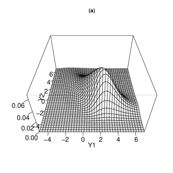
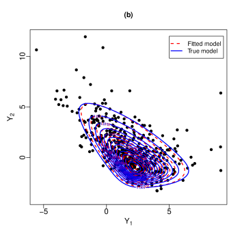
Figure 8.7: The PDF of $\text{SGG}_{2,2}(\bm{\mu},\Sigma,{\Lambda},\bm{\theta})$. (a): true model and (b): true and fitted contour plots.

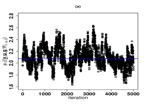
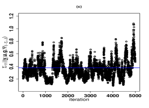
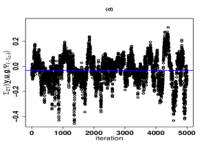
Figure 8.8: Scatterplot of 10000 samples generated from full conditionals involved in Bayesian paradigm of $\text{SGG}_{2,2}(\bm{\mu},\Sigma,{\Lambda},\bm{\theta})$.

8.5 Gibbs sampling in Bayesian paradigm with more than two latent variable: Model-based Clustering

The aim of clustering technique is to divide a non-homogeneous population into K numbers of homogeneous sub-populations. Obviously, members of a non-homogeneous population have dissimilarities while the clustered or partitioned sub-populations have more similarities. Herein, the term “similarity” may refer to some measurable attribute or criterion such as Euclidean distance. If two observations are similar, then they are close together (high degree of similarity) and otherwise, two observations are dissimilar (low degree of similarity).

Figure 8.9: (a): Ten data points that can constitute a cluster, (b): Ten data points that should be clustered into two groups, (c): Ten data points in part (a) that can be modelled through a single-component (homogeneous) model with PDF $f\bigl{(}\bm{y}\bigl{|}\bm{\Theta}\bigr{)}$, and (d): Ten data points in part (b) that can be modelled through a two-component (non-homogeneous) mixture model with PDF $0.4f\bigl{(}\bm{y}\bigl{|}\bm{\Theta}_{1}\bigr{)}+0.6f\bigl{(}\bm{y}\bigl{|}\bm{\Theta}_{2}\bigr{)}$.

Figure 8.9(a) displays a set of ten observations, labeled with numbers $1,2,\cdots,10$, that are similar and so can constitute a cluster. On the other hand, consider the situation in which ten observations are non-homogeneous or dissimilar as shown by Figure 8.9(b). Herein, ten observations with labels $\{7,6,1,4\}$ are similar together, but quite dissimilar with observations whose label are $\{2,8,1,3,9,5\}$. So, observations in Figure 8.9(b) should be groped into two clusters. We emphasize that the objective of clustering technique is to determine the label of each observation. Furthermore, sometimes the yardstick for measuring the similarity between observations may not be a quantitative tool such as the Euclidean distance. The clustering technique proceeds to divide observations into K groups such that the observations within each group have the maximum degree of similarity while the observations between groups have the maximum degree of dissimilarity. Sometimes the clustering technique is known as semi-supervised or unsupervised machine learning since label of observations are not known and the only available information are observed data McNicholas (2016).

The model-based clustering (or non-hierarchical clustering) uses a finite mixture of multivariate statistical distributions of the same family for the purpose of clustering. Hence, the model-based clustering and finite mixture models are often used interchangeably in the literature. As mentioned above, the aim of clustering is to determine the label or the origin of an observation is coming from. It is worth to note that the concepts “origin”, “cluster”, “label”, and “component” may be used interchangeably. For more clarifications, Figure 8.9(c) shows a set of ten observations with perfect similarity and, within the model-based clustering framework, we assume that these ten observations follow independently the same multivariate distribution. On the other hand, Figure 8.9(d) shows another set of ten observations with two clusters, and hence within the model-based clustering framework, we prefer to assume these data points are coming from two different multivariate statistical distribution of the same family. In other words, for the first and second clusters we consider two multivariate statistical distributions of the same family whose PDFs are $f\bigl{(}\bm{y}\bigl{|}\bm{\Theta}_{1}\bigr{)}$ and $f\bigl{(}\bm{y}\bigl{|}\bm{\Theta}_{2}\bigr{)}$, respectively. The corresponding weights are 0.4 and 0.6 and hence the distribution of ten observations is a mixture of two distributions fitted to two clusters whose PDF is

$$g(\bm{y}|\bm{\Psi})=0.4f\bigl{(}\bm{y}\bigl{|}\bm{\Theta}_{1}\bigr{)}+0.6f\bigl{(}\bm{y}\bigl{|}\bm{\Theta}_{2}\bigr{)}.$$ (8.55)

In (8.55), the vector $\bm{\omega}=(0.40,0.60)^{\top}$, is known as the weight vector that means 40% of observations in Figure 8.9(d) are coming from the first component and the remaining 60% are coming from the second component. Overall, for $p$-dimensional random vector $\bm{Y}$, the PDF of a K-component mixture model is given by

$$g(\bm{y}|\bm{\Psi})=\sum_{k=1}^{\text{K}}\omega_{k}f\bigl{(}\bm{y}\bigl{|}\bm{\Theta}_{k}\bigr{)},$$ (8.56)

where $\bm{\Psi}=(\bm{\omega}^{\top},\bm{\Theta}_{1},\cdots,\bm{\Theta}_{\text{K}})$ is the parameter space in which $\bm{\omega}=(\omega_{1},\dots,\omega_{\text{K}})^{\top}$ is vector of mixing parameters such that $\sum_{k=1}^{\text{K}}\omega_{k}=1$. In (8.56), $f_{\bm{Y}}(\bm{y}|\bm{\Theta}_{k})$ is the PDF of $k$-th component and hence the PDF $g(\bm{y}|\bm{\Psi})$ is proper since

$$\int_{\mathbb{R}^{p}}g(\bm{y}|\bm{\Psi})d\bm{y}=\sum_{k=1}^{\text{K}}\omega_{k}\int_{\mathbb{R}^{p}}f\bigl{(}\bm{y}\bigl{|}\bm{\Theta}_{k}\bigr{)}d\bm{y}=\sum_{k=1}^{\text{K}}\omega_{k}=1.$$

The weight parameter $\bm{\omega}$ provides the chance of observing sample from components. Sometimes, representation (8.56) is called the finite mixture model since the quantity K or number of clusters is assumed to be finite. In next two subsections, we proceed to discuss about generating realization from a finite mixture model and how to determine quantity K.

8.5.1 Generating from Gaussian finite mixture model

For generating $n$ realizations from a K-component mixture model, we may follow one of the two following approaches. In the first method, one can generate independently $n_{k}=\lceil n\times\omega_{k}\rceil$ (for $k=1,\cdots,{\text{K}}-1$) realizations from PDF $f\bigl{(}\bm{y}\big{|}\bm{\Theta}_{k}\bigr{)}$ in which $\lceil n\times\omega_{k}\rceil$ denotes the smallest integer value equal or greater than $n\times\omega_{k}$, and finally $n_{\text{K}}=n-\sum_{k=1}^{{\text{K}}-1}n_{k}$ realizations are drawn independently from PDF $f\bigl{(}\bm{y}\big{|}\bm{\Theta}_{\text{K}}\bigr{)}$. Herein, we represent the multinomial distribution. If random vector $\bm{X}=(X_{1},\cdots,X_{\text{K}})^{\top}$ follows a multinomial distribution, then its PDF is given by

$${\cal{MUL}}\bigl{(}\bm{x}\big{|}n,\bm{\omega}\bigr{)}=\frac{\Gamma(n+1)}{\prod_{k=1}^{{\text{K}}}\Gamma\bigl{(}n_{k}+1\bigr{)}}\omega_{1}^{x_{1}}\omega_{2}^{x_{2}}\cdots\omega_{{\text{K}}}^{x_{{\text{K}}}},$$ (8.57)

where $\bm{\omega}=\bigl{(}\omega_{1},\cdots,\omega_{\text{K}}\bigr{)}^{\top}$ is distribution’s parameter vector, $n=\sum_{k=1}^{{\text{K}}}x_{k}$, and $\omega_{k}>0$ provided that $\sum_{k=1}^{{\text{K}}}\omega_{k}=1$. We write $\bm{X}\sim{\cal{MUL}}(n,\bm{\omega})$ to indicate that random vector $\bm{X}$ follows a multinomial distribution with PDF given by (8.57). Moreover, if random vector $\bm{X}=(X_{1},\cdots,X_{\text{K}})^{\top}$ follows a Dirichlet distribution with parameter vector $\bm{\rho}$, say $\bm{X}\sim{\cal{DIR}}(\bm{\rho})$, then the PDF of $\bm{X}$ is

$${\cal{DIR}}(\bm{x}|\bm{\rho})=\frac{\Gamma\bigl{(}\rho_{1}+\cdots+\rho_{{\text{K}}}\bigr{)}}{\prod_{k=1}^{{\text{K}}}\Gamma\bigl{(}\rho_{k}\bigr{)}}x_{1}^{\rho_{1}-1}\times x_{2}^{\rho_{2}-1}\times\cdots\times x_{{\text{K}}}^{\rho_{\text{K}}-1},$$ (8.58)

where $0<x_{k}<1$ and ${\rho}_{k}>0$ (for $k=1,\cdots,{\text{K}}$), provided that $\sum_{k=1}^{{\text{K}}}x_{k}=1$. The following pseudo code describes how to draw a sample of size $n$ from a K-component Gaussian mixture model under the second method.

Algorithm 8 Simulating from a mixture model-2

1:Read $n$, K (number of components), and $\bm{\Psi}=(\bm{\omega},\bm{\Theta}_{1},\cdots,\bm{\Theta}_{\text{K}})$;

2:Set $\bm{Y}$ a vector of length $n$;

3:Set $i=1$;

4:while $i\leq n$ do

5:     Sample $\bm{u}\sim{\cal{MUL}}(1,\bm{\omega})$;

6:     Set $k_{max}=\bigl{\{}k|\bm{u}[k]=1\bigr{\}}$ where $\bm{u}[k]$ is the $k$th element of vector $\bm{u}$ for

7:     $k=1,\cdots,{\text{K}}$;

8:     Sample $\bm{y}$ from PDF $f\bigl{(}\cdot\bigl{|}\bm{\Theta}_{k_{max}}\bigr{)}$

9:     Set $\bm{Y}[i]\leftarrow\bm{y}$;

10:     Set $i\leftarrow i+1$;

11:end

12:Accept $\bm{Y}$ as sample of size $n$ from K-component mixture model.

Example 24 Suppose we are interested in generating a sample of $n=300$ observations from observations are coming from a three-component bivariate Gaussian mixture model with PDF given by

$$g(\bm{y}|\bm{\Psi})=\frac{1}{3}{\cal{N}}_{2}\bigl{(}\bm{\mu}_{1},\Sigma_{1}\bigr{)}+\frac{1}{3}{\cal{N}}_{2}\bigl{(}\bm{\mu}_{2},\Sigma_{2}\bigr{)}+\frac{1}{3}{\cal{N}}_{2}\bigl{(}\bm{\mu}_{3},\Sigma_{3}\bigr{)},$$ (8.59)

where $\bm{\Psi}=\bigl{(}\omega_{1},\omega_{2},\omega_{3},\Theta_{1},\Theta_{2},\Theta_{3}\bigr{)}$ is whole parameter vector whose elements are

$$\Theta_{1}=\omega_{1}=\frac{1}{3},\bm{\mu}_{1}=(-3,-3)^{\top},\Sigma_{1}=\biggl{[}\begin{matrix}1&0.5\\ 0.5&1\end{matrix}\biggr{]},$$

$$\Theta_{2}=\omega_{2}=\frac{1}{3},\bm{\mu}_{2}=(0,0)^{\top},\leavevmode\nobreak\ \leavevmode\nobreak\ \leavevmode\nobreak\ \leavevmode\nobreak\ \leavevmode\nobreak\ \Sigma_{2}=\biggl{[}\begin{matrix}1&0\\ 0&1\end{matrix}\biggr{]},$$

$$\Theta_{3}=\omega_{3}=\frac{1}{3},\bm{\mu}_{3}=(3,3)^{\top},\leavevmode\nobreak\ \leavevmode\nobreak\ \leavevmode\nobreak\ \leavevmode\nobreak\ \leavevmode\nobreak\ \Sigma_{3}=\biggl{[}\begin{matrix}1&-0.25\\ -0.25&1\end{matrix}\biggr{]}.$$ (8.60)

Based on Algorithm 8, we use the following R code to generate from three-component bivariate Gaussian mixture model with whole parameter given as above. Figure 8.10(a) displays the corresponding scatterplot.

⬇

1R> library(MASS) # for generating realization from multivariate Gaussian

2R> set.seed(20240713)

3R> K <- 3

4R> omega <- rep(1/3, K)

5R> Mu1 <- rep(-3, p); Mu2 <- rep(0, p); Mu3 <- c(3, -3)

6R> Sigma1 <- diag(0.5, p) + matrix(.5, p, p)

7R> Sigma2 <- diag(1, p)

8R> Sigma3 <- diag(1.5, p) + matrix(-0.5, p, p)

9R> Sigma2 <-matrix(c(1, 0, 0, 1), 2, 2);

10R> Sigma3 <-matrix(c(1,-0.25,-0.25,1), 2, 2);

11R> Mu <- list(Mu1, Mu2, Mu3)

12R> Sigma <- list(Sigma1, Sigma2, Sigma3)

13R> rmixnorm <- function(n, Mu, Sigma, omega)

14+ {

15+ p <- length( Mu[[1]] )

16+ label <- rep(0, n)

17+ Y <- matrix(0, nrow = n, ncol = p)

18+ for(i in 1:n)

19+ {

20+ r_MUL <- rmultinom(n = 1, size = 1, omega)

21+ k <- apply(r_MUL, 2, which.max)

22+ label[i] <- k

23+ Y[i, ] <- mvrnorm(n = 1, mu = Mu[[k]], Sigma = Sigma[[k]])

24+ }

25+ ls <- list( "sample" = Y, "label" = label )

26+ return(ls)

27+ }

28R> Y <- rmixnorm(n, Mu, Sigma, omega)

29R> plot( Y$sample, col = Y$label )

8.5.2 Model selection

The true value of K is not known in practice. This quantity can be determined through the Bayesian information criterion (BIC) (Schwarz et al., 1978). The process of finding best K is known as the model selection in the literature. Based on $n$ realizations $\bm{y}_{1},\cdots,\bm{y}_{n}$ that are assumed to follow independently a distribution with PDF $g(\bm{y}|\bm{\Psi})$, the BIC is defined as

$$\text{BIC}=2\sum_{i=1}^{n}\log\sum_{k=1}^{{\text{K}}}\widehat{\omega_{k}}f\bigl{(}\bm{y}_{i}\big{|}\widehat{\bm{\Theta}_{k}}\bigr{)}-N\log n,$$ (8.61)

where $\widehat{{\omega}_{k}}$ and $\widehat{\bm{\Theta}_{k}}$ (for $k=1,\cdots,{{\text{K}}}$) account for the ML estimators of ${{\omega}}_{k}$ and ${\bm{\Theta}}_{k}$, respectively. Furthermore, constant $N$ denotes number of model’s free parameters that must be estimated. The BIC is an effective criterion for model selection in Gaussian mixture models, see Fraley and Raftery (2002); Mcnicholas and Murphy (2008), and has been used frequently for other model-based clustering, seeKeribin (2000); Fraley and Raftery (1998, 2002); Mcnicholas and Murphy (2008); McNicholas and Murphy (2010). In practice, for determining K, we compute BIC defined by (8.61) when data points are clustered through other clustering approaches such as k-mean (Hartigan and Wong, 1979) or other approaches of clustering, for $k=1,2,\cdots$. We choose the mixture model for which BIC is the largest. For instance, suppose that we do not know the true value of K when 300 observations are coming from a three-component bivariate Gaussian mixture model with true parameters given by (8.5.1). As expected, when ${{\text{K}}}=3$ the BIC gets its maximum value, see Figure 8.10(b). The R function BIC has been developed for determining the true value of K for a K-component Gaussian mixture model.

⬇

1R> dmvnorm <- function(x, mean, sigma)

2+ {

3+ p <- length(mean)

4+ 1/sqrt((2*pi)^p*det(sigma))*exp(-mahalanobis(x, mean, sigma)/2)

5+ }

6R> BIC <- function(Y, param = NULL, k_max = 6)

7+ {

8+ dim_y <- dim(Y)

9+ n <- dim_y[1]

10+ p <- dim_y[2]

11+ if( is.null(param) )

12+ {

13+ bic <- rep(0, k_max)

14+ for(k in 1:k_max)

15+ {

16+ Mu_hat <- matrix(0, nrow = k, ncol = p)

17+ Sigma_hat <- array(0, dim = c(p, p, k) )

18+ N <- (k - 1) + k*( p + p*(p + 1)/2 )

19+ cluster <- kmeans(Y, k)

20+ omega <- cluster$size/n

21+ Sum_bic <- matrix(0, nrow = n, ncol = k)

22+ for(i in 1:k)

23+ {

24+ clust <- Y[cluster$cluster == i, ]

25+ Mu_hat[i,] <- apply(clust, 2, mean)

26+ Sigma_hat[,,i] <- cov(clust)

27+ Sum_bic[, i] <- omega[i]*dmvnorm(Y, mean = Mu_hat[i,],

28+ sigma = Sigma_hat[,,i])

29+ }

30+ bic[k] <- 2*sum( log( apply(Sum_bic, 1, sum) ) ) - N*log(n)

31+ }

32+ out <- data.frame(k = 1:k, bic = bic)

33+ ls <- list( "model" = out, "K" = which.max(bic) )

34+ }else{

35+ omega <- param[[1]]

36+ Mu <- param[[2]]

37+ Sigma <- param[[3]]

38+ K <- length( Mu )

39+ Sum_bic <- matrix(0, nrow = n, ncol = K)

40+ N <- (K - 1) + K*( p + p*(p + 1)/2 )

41+ for(k in 1:K)

42+ {

43+ Sum_bic[, k] <- omega[k]*dmvnorm(Y, mean = Mu[[k]],

44+ sigma = Sigma[[k]])

45+ }

46+ out <- 2*sum( log( apply(Sum_bic, 1, sum) ) ) - N*log(n)

47+ ls <- list( "bic" = out, "K" = K )

48+ }

49+ return(ls)

50+ }

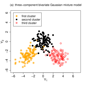
Figure 8.10: (a): Scatterplot of 300 data points drawn from $\bm{Y}=(Y_{1},Y_{2})^{\top}$ following a three-component Gaussian mixture model and (b): Computed BIC versus number of clusters.

As noted earlier, determining the label of each observation is the main task of each clustering technique. To this end, we may use the Bayesian (Gibbs sampling) or the expectation-maximization (EM) (Dempster et al., 1977) algorithm. If the former applied, depending on the model structure, the Gibbs sampling involves one, two, or more latent variables.

8.6 Finite mixture of Gaussian distributions

Evidently the most commonly used statistical distribution for the purpose of model-based clustering is Gaussian mixture model. Suppose $p$-dimensional random vector $\bm{Y}$ follows a K-component Gaussian mixture model. It is clear that

$$\bm{Y}\big{|}H_{ik}=1 \sim{\cal{N}}_{p}\bigl{(}\bm{\mu}_{k},\Sigma_{k}\bigr{)},$$

$$\bm{H}_{i} \sim{\cal{MUL}}\bigl{(}\bm{\omega}\big{|}1\bigr{)}.$$

Since $\bm{H}_{i}$ is latent variable, hence we encounter with a incomplete data problem. Here $\{\bm{y}_{1},\cdots,\bm{y}_{n}\}$ is the sequence of observed data and $\bm{H}_{i}=(H_{i1},\cdots,H_{i\text{K}})^{\top}$ is the missing component’s label. Herein ${H}_{ik}=1$ takes on values zero and one. If ${H}_{ik}=1$, then $\bm{y}_{i}$ comes from $k$-th component, otherwise $H_{i1}=0$. Hence, the complete data PDF can be represented as

$$g_{c}({\underline{\bm{y}}}|\bm{\Psi})=\prod^{n}_{i=1}g\bigl{(}\bm{y}_{i},\bm{H}_{i}\big{|}\bm{\Psi}\bigr{)},$$ (8.62)

where ${\underline{\bm{y}}}=\{\bm{y}_{1},\cdots,\bm{y}_{n}\}$ and

$$g\bigl{(}\bm{y}_{i},\bm{H}_{i}\big{|}\bm{\Psi}\bigr{)} =g\bigl{(}\bm{y}_{i}\big{|}\bm{H}_{i},\bm{\Psi}\bigr{)}\times{\cal{MUL}}\bigl{(}\bm{\omega}\big{|}1\bigr{)}$$

$$=\biggl{[}{\cal{N}}_{p}\Bigl{(}\bm{y}_{i}\Big{|}\bm{\mu}_{k},\Sigma_{k}\Bigr{)}\biggr{]}^{H_{ik}}\times\omega_{1}^{H_{i1}}\times\cdots\times\omega_{{\text{K}}}^{H_{i{\text{K}}}}$$

$$=\prod_{k=1}^{{\text{K}}}\biggl{[}\omega_{k}{\cal{N}}_{p}\Bigl{(}\bm{y}_{i}\Big{|}\bm{\mu}_{k},\Sigma_{k}\Bigr{)}\biggr{]}^{H_{ik}}.$$ (8.63)

Replacing the RHS of (8.6) into the RHS of (8.62), the PDF of complete-data is

$$g_{c}({\underline{\bm{y}}}|\bm{\Psi})=\prod^{n}_{i=1}\prod_{k=1}^{{\text{K}}}\biggl{[}\omega_{k}{\cal{N}}_{p}\Bigl{(}\bm{y}_{i}\Big{|}\bm{\mu}_{k},\Sigma_{k}\Bigr{)}\biggr{]}^{H_{ik}}.$$ (8.64)

Thus, the complete-data likelihood function is

$$L_{c}(\bm{\Psi}|{\underline{\bm{y}}},\underline{\bm{H}})= (2\pi)^{-\frac{np}{2}}\times\omega_{k}^{\sum_{i=1}^{n}H_{ik}}\times\cdots\times\omega_{{\text{K}}}^{\sum_{i=1}^{n}H_{i{\text{K}}}}\times\big{|}\Sigma_{k}\big{|}^{-\frac{\sum_{i=1}^{n}\sum_{k=1}^{{\text{K}}}H_{ik}}{2}}$$

$$\times\exp\Bigl{\{}-\frac{1}{2}\sum_{i=1}^{n}\sum_{k=1}^{{\text{K}}}H_{ik}\bigl{(}\bm{y}_{i}-\bm{\mu}_{k}\bigr{)}^{\top}\Sigma^{-1}_{k}\bigl{(}\bm{y}_{i}-\bm{\mu}_{k}\bigr{)}\Bigr{\}},$$

$$\propto \omega_{1}^{n_{1}}\times\cdots\times\omega_{{\text{K}}}^{n_{\text{K}}}\times\big{|}\Sigma_{1}\big{|}^{-\frac{n_{1}}{2}}\times\cdots\times\big{|}\Sigma_{{\text{K}}}\big{|}^{-\frac{n_{{\text{K}}}}{2}}$$

$$\times\exp\Bigl{\{}-\frac{1}{2}\sum_{i=1}^{n}\sum_{k=1}^{{\text{K}}}H_{ik}\bigl{(}\bm{y}_{i}-\bm{\mu}_{k}\bigr{)}^{\top}\Sigma^{-1}_{k}\bigl{(}\bm{y}_{i}-\bm{\mu}_{k}\bigr{)}\Bigr{\}},$$ (8.65)

where $\underline{\bm{H}}=\{\bm{H}_{1},\cdots,\bm{H}_{n}\}$ in which $\bm{H}_{i}=(H_{i1},\cdots,H_{i\text{K}})^{\top}$ and $n_{k}=\sum_{i=1}^{n}H_{ik}$ provided that $n=\sum_{k=1}^{{\text{K}}}n_{k}$. Given $i$th observed data $\bm{y}_{i}$, for computing PDF of $\bm{H}_{i}|\bm{Y}=\bm{y}_{i}$, it follows from (8.6) that

$$L_{c}\bigl{(}\bm{\Psi}\big{|}{\bm{y}}_{i},{\bm{H}}_{i}\bigr{)}\propto g\bigl{(}\bm{y}_{i}\big{|}\bm{H}_{i},\bm{\Psi}\bigr{)}\times{\cal{MUL}}\bigl{(}\bm{\omega}\big{|}1\bigr{)}.$$

Obviously,

$$\bm{H}_{i}\big{|}\bm{\Psi},\bm{Y}=\bm{y}_{i}\sim{\cal{MUL}}\bigl{(}\bm{\tau}_{i}\big{|}1\bigr{)},$$ (8.66)

where $\bm{\tau}_{i}=(\tau_{i1},\cdots,\tau_{i\text{K}})^{\top}$ denotes the $i$th row of $n\times{\text{K}}$ matrix $\bm{\tau}$ whose $(i,k)$th element is

$${\tau}_{i,k}=\frac{\omega_{k}{\cal{N}}_{p}\bigl{(}\bm{y}_{i}\big{|}\bm{\mu}_{k},\Sigma_{k}\bigr{)}}{\sum_{k=1}^{\text{K}}\omega_{k}{\cal{N}}_{p}\bigl{(}\bm{y}_{i}\big{|}\bm{\mu}_{k},\Sigma_{k}\bigr{)}}.$$ (8.67)

Once we have generated the entire sample (for $i=1,\cdots,n$) from full conditional $\bm{H}_{i}\big{|}\bigl{(}\bm{\Psi},{\bm{y}}_{i}\bigr{)}$, we proceed to generate from full conditionals $\bm{\mu}_{k}\big{|}\bigl{(}{\underline{\bm{y}}},\underline{\bm{H}},\bm{\Psi}_{(-\bm{\mu}_{k})}\bigr{)}$ and $\Sigma_{k}\big{|}\bigl{(}{\underline{\bm{y}}},\underline{\bm{H}},\bm{\Psi}_{(-{\Sigma}_{k})}\bigr{)}$ (for $k=1,\cdots,{\text{K}}$). To this end, first we have

$$\pi(\bm{\Psi}|{\underline{\bm{y}}},\underline{\bm{H}}) \propto L_{c}(\bm{\Psi}|\underline{\bm{y}},\underline{\bm{H}})\times\pi\bigl{(}\bm{\Psi}_{1}\bigr{)}\times\cdots\times\pi\bigl{(}\bm{\Psi}_{{\text{K}}}\bigr{)}$$

$$=L_{c}(\bm{\Psi}|\underline{\bm{y}},\underline{\bm{H}})\times\pi\bigl{(}\bm{\omega}\bigr{)}\times\pi\bigl{(}\bm{\mu}_{1}\bigr{)}\times\cdots\times\pi\bigl{(}\bm{\mu}_{{\text{K}}}\bigr{)}\times\pi\bigl{(}\Sigma_{1}\bigr{)}\times\cdots\times\pi\bigl{(}\Sigma_{{\text{K}}}\bigr{)}.$$ (8.68)

Substituting $L_{c}(\bm{\Psi}|\underline{\bm{y}},\underline{\bm{H}})$ given by (8.6) into the RHSS of (8.6) yields

$$\pi(\bm{\Psi}|{\underline{\bm{y}}},\underline{\bm{H}})\propto \times\pi\bigl{(}\bm{\omega}\bigr{)}\times\pi\bigl{(}\bm{\mu}_{1}\bigr{)}\times\cdots\times\pi\bigl{(}\bm{\mu}_{{\text{K}}}\bigr{)}\times\pi\bigl{(}\Sigma_{1}\bigr{)}\times\cdots\times\pi\bigl{(}\Sigma_{{\text{K}}}\bigr{)}\times$$

$$\omega_{1}^{n_{1}}\times\cdots\times\omega_{{\text{K}}}^{n_{\text{K}}}\times\big{|}\Sigma_{1}\big{|}^{-\frac{n_{1}}{2}}\times\cdots\times\big{|}\Sigma_{{\text{K}}}\big{|}^{-\frac{n_{{\text{K}}}}{2}}$$

$$\times\exp\Bigl{\{}-\frac{1}{2}\sum_{i=1}^{n}\sum_{k=1}^{{\text{K}}}H_{ik}\bigl{(}\bm{y}_{i}-\bm{\mu}_{k}\bigr{)}^{\top}\Sigma^{-1}_{k}\bigl{(}\bm{y}_{i}-\bm{\mu}_{k}\bigr{)}\Bigr{\}}.$$ (8.69)

We consider, for $k=1,\cdots,{\text{K}}$, independent conjugate priors as follows.

$$\pi(\bm{\omega}) \sim{\cal{DIR}}\bigl{(}\bm{\rho}\bigr{)},$$ (8.70)

$$\pi\bigl{(}\bm{\mu}_{k}\bigr{)} \sim{\cal{N}}_{p}\bigl{(}{\cal{M}}_{k},{\cal{S}}_{k}\bigr{)},$$ (8.71)

$$\pi\bigl{(}\Sigma_{k}\bigr{)} \sim{\cal{IW}}\bigl{(}{\cal{D}}_{k},\nu_{k}\bigr{)},$$ (8.72)

where ${\cal{DIR}}\bigl{(}\cdot\bigr{)}$ is defined in (8.58). In what follows, we give the full conditionals needed for implementing the Gibbs sampling.

• full conditional of $\bm{\omega}\big{|}\bigl{(}{\underline{\bm{y}}},\underline{\bm{H}},\bm{\Psi}_{(-\bm{\omega})}\bigr{)}$: Substituting prior $\pi(\bm{\omega})$ given by (8.6) into the RHS of (8.6) yields

  $$\pi\bigl{(}\bm{\omega}\big{|}{\underline{\bm{y}}},\underline{\bm{H}},\bm{\Psi}_{(-\bm{\mu})}\bigr{)} \propto{\cal{DIR}}\bigl{(}\bm{\omega}\big{|}\bm{\rho}\bigr{)}\times\omega_{1}^{n_{1}}\times\cdots\times\omega_{{\text{K}}}^{n_{\text{K}}}={\cal{DIR}}\bigl{(}\bm{\omega}\big{|}\bm{\rho}_{*}\bigr{)},$$

  where

  $$\bm{\rho}_{*}=\Bigl{(}\rho_{1}+\sum_{i=1}^{n}H_{i1},\cdots,\rho_{{\text{K}}}+\sum_{i=1}^{n}H_{i{\text{K}}}\Bigr{)}^{\top}.$$

• full conditional of $\bm{\mu}_{k}\big{|}\bigl{(}{\underline{\bm{y}}},\underline{\bm{H}},\bm{\Psi}_{(-\bm{\mu}_{k})}\bigr{)}$: Substitute the prior $\pi\bigl{(}\bm{\mu}_{k}\bigr{)}$ given by (8.70) into the RHS of (8.6). Then more algebra shows

  $$\pi\bigl{(}\bm{\mu}\big{|}{\underline{\bm{y}}},\underline{\bm{H}},\bm{\Psi}_{(-\bm{\mu}_{k})}\bigr{)}={\cal{N}}_{p}\Bigl{(}\bm{\mu}\Big{|}{\cal{Q}}_{k}\Bigl{[}{\cal{S}}^{-1}_{k}{\cal{M}}_{k}+\Sigma_{k}^{-1}\sum_{i=1}^{n}H_{ik}\bm{y}_{i}\Bigr{]},{\cal{Q}}_{k}\Bigr{)},$$

  where

  $${\cal{Q}}_{k}=\Bigl{[}{\cal{S}}^{-1}_{k}+\Sigma_{k}^{-1}\times\sum_{i=1}^{n}H_{ik}\Bigr{]}^{-1}.$$

• full conditional of ${\Sigma}_{k}\big{|}\bigl{(}{\underline{\bm{y}}},\underline{\bm{H}},\bm{\Psi}_{(-\Sigma_{k})}\bigr{)}$: Substitute the prior $\pi\bigl{(}{\Sigma}_{k}\bigr{)}$ given by (8.71) into the RHS of (8.6). Then more algebra shows

  $$\pi\bigl{(}{\Sigma}\big{|}{\underline{\bm{y}}},\underline{\bm{H}},\bm{\Psi}_{(-{\Sigma}_{k})}\bigr{)}\sim{\cal{IW}}\bigl{(}{\cal{R}}_{k},\nu_{k}+\sum_{i=1}^{n}H_{ik}\bigr{)},$$

  where ${\cal{R}}_{k}={\cal{D}}_{k}+\sum_{i=1}^{n}H_{ik}\bigl{(}\bm{y}_{i}-\bm{\mu}_{k}\bigr{)}\bigl{(}\bm{y}_{i}-\bm{\mu}_{k}\bigr{)}^{\top}$.

The following pseudo code gives the details for implementing the model-based clustering for finite mixture of Gaussian distributions.

Algorithm 9 Bayesian inference for finite mixture of Gaussian distributions

1:Read $N$, $M$, and determine quantities K, ${\omega}_{k}$, ${\cal{M}}_{k}$, ${\cal{S}}_{k}$, ${\cal{D}}_{k}$, $\nu_{k}$, for $k=1\cdots,{\text{K}}$

2:Set $t=0$;

3:Determine initial values $\bm{\omega}^{(0)}$, $\bm{\mu}^{(0)}$, $\Sigma^{(0)}$, and set $\bm{\Psi}^{(0)}=\bigl{(}\bm{\omega}^{(0)}$,$\bm{\mu}^{(0)},\Sigma^{(0)}\bigr{)}$;

4:while $t\leq N$ do $\triangleright$ start Gibbs sampling

5:     Set $i=1$;

6:     while $i\leq n$ do $\triangleright$ start for sampling form missing labels

7:         Simulate the $i$ row of $n\times{\text{K}}$ matrix $\bm{H}$ as $\bm{H}_{i}\sim{\cal{MUL}}\bigl{(}\cdot\big{|}\bm{\tau}_{i}\bigr{)}$ where

8:         $\bm{\tau}_{i}=(\tau_{i1},\ldots,\tau_{i\text{K}})^{\top}$ is the $i$th row of matrix $\bm{\tau}$ is given by (8.67);

9:         Set $i=i+1$;      

10:     end

11:     Set, for $k=1,\cdots,{\text{K}}$, $n_{k}=\sum_{i=1}^{n}H_{i,k}$ where $H_{i,k}$ denotes the $(i,k)$th

12:     element of $\bm{H}$;

13:     Simulate $\bm{\omega}\sim{\cal{DIR}}\bigl{(}1|\rho_{*}\bigr{)}$ where $\rho_{*}=(\rho_{1}+n_{1},\cdots,\rho_{{\text{K}}}+n_{{\text{K}}})^{\top}$;

14:     Set $k=1$;

15:     while $k\leq K$ do $\triangleright$ start sampling from full conditionals of $\bm{\mu}_{k}$, and $\Sigma_{k}$

16:         Generate $\bm{\mu}_{k}^{(t+1)}\sim{\cal{N}}_{p}\Bigl{(}{\cal{Q}}_{k}\Bigl{[}{\cal{S}}^{-1}_{k}{\cal{M}}_{k}+\bigl{[}\Sigma_{k}^{(t)}\bigr{]}^{-1}\sum_{i=1}^{n}H_{i,k}\times\bm{y}_{i}\Bigr{]},{\cal{Q}}_{k}\Bigr{)}$

17:         where ${\cal{Q}}_{0}=\Bigl{[}{\cal{S}}^{-1}_{0}+\bigl{[}\Sigma_{k}^{(t)}\bigr{]}^{-1}\times n_{k}\Bigr{]}^{-1}$;

18:         Generate $\Sigma_{k}^{(t+1)}$ from ${\cal{IW}}\bigl{(}{\cal{R}}_{k},\nu_{k}+n_{k}\bigr{)}$ where ${\cal{R}}_{k}={\cal{D}}_{k}+\sum_{i=1}^{n}H_{i,k}\times$

19:         $\bigl{(}\bm{y}_{i}-\bm{\mu}_{k}^{(t+1)}\bigr{)}\bigl{(}\bm{y}_{i}-\bm{\mu}_{k}^{(t+1)}\bigr{)}^{\top}$;

20:         Set $k=k+1$;      

21:     end

22:     Set $\bm{\Psi}^{(t+1)}=\bigl{(}\bm{\omega}^{(t+1)},\bm{\mu}_{1}^{(t+1)}\cdots,\bm{\mu}_{{\text{K}}}^{(t+1)},\Sigma_{1}^{(t+1)},\cdots,\Sigma_{{\text{K}}}^{(t+1)}\bigr{)}$ and $t=t+1$;

23:end

24:Sequence $\bigl{\{}\bm{\Psi}^{(M+1)},\cdots,\bm{\Psi}^{(N)}\bigr{\}}$ is a sample of size $N-M$ from

25:posterior $\pi\bigl{(}\bm{\Psi}|{\underline{\bm{y}}},\underline{\bm{H}}\bigr{)}$;

26:The Bayesian estimator of $\bm{\Psi}$ is given by $\frac{1}{N-M}\sum_{t=1}^{N-M}\bm{\Psi}^{(t)}$.

While Algorithm 9 works reasonably well, its performance is subject to outliers. If clusters have large variances, then the Gibbs sampling may fail to allocate true label to each cluster. This mainly because this fact that Gaussian distribution has light tails and the PDF decays exponentially for observation are far from the center of distribution. For instance, consider a two-component bivariate mixture model with equal weights $\omega_{1}=\omega_{2}=0.5$ while the second cluster has large locations and variances. It is easy to check that the elements of second column of matrix $\bm{\tau}$ in (8.67) are very small and hence, $P(H_{i,2}=1)\rightarrow 1$ for $i=1,\cdots,n$. Hence, all observations are allocated to the first cluster. One way to tackle this issue is standardization of observations before clustering (Tortora et al., 2021). The following example gives more detailed information about this case.

Example 25 Herein, we are interested in clustering the famous Old Faithful Geyser Data (known as faithful data). This faithful data consists of 272 observations on two variables duration of the eruption in minutes and waiting time between eruptions for the Old Faithful geyser in Yellowstone National Park, Wyoming, USA, (Azzalini and Bowman, 1990). Figure 8.11(a) displays the scatterplot of this dataset. Our investigation shows that the BIC of -833.7747 suggests that ${\text{K}}=2$ for which the k-mean algorithm pre-clustering results shows that the variances of second variable in both clusters are significantly large as 31.66 and 34.75. Using the R code after standardization given by

R> data(faithful)
R> Y <- matrix( cbind(faithful$eruptions, faithful$waiting),
+Ψ      nrow = 272, ncol = 2)
R> Z <- apply( Y, 2, function(x)( x - mean(x) )/sd(x) )
R> bic <- BIC(Z)
R> out_kmeans <- kmeans(Z, bic$K)
R> label <- out_kmeans$cluster
R> sapply(1:K, function(x) var( Z[label == x, ] ))

then, it can be seen that variances of second variable in both clusters are 0.1876 and 0.1874, correspondingly. The R package mclust (Scrucca et al., 2016) applies the EM algorithm for model-based clustering based on the finite mixture of Gaussian distributions. We notice that the clustering results based on both the Gibbs sampling proposed here and EM algorithm proposed in (Scrucca et al., 2016) are the same. The most commonly used criterion for measuring the degree of agreement between clustering approaches is the adjusted Rand index (ARI) that varies from 0 (for zero agreement in clustering) to 1 (for perfect agreement in clustering) (Hubert and Arabie, 1985). Herein, we use the ARI to compare the Bayesian paradigm and EM algorithm for clustering the faithful data. To this end, among several R packages that can compute the ARI, we call the package MixGHD. Fortunately, the agreement between two above approaches in clustering faithful data is perfect, that is ARI=1. Figure 8.11(b) and (c) display the contour and scatterplot fitted to standardized faithful data. The R function FGM given by the following can be used for applying the model-based clustering to the Gaussian finite mixture model.

⬇

1R> FMG <- function(Y, K, n_burn, n_sim, param, hyper = NULL, scale = FALSE )

2+ {

3+ if( scale == TRUE ) Y <- apply( Y, 2, function(x)( x - mean(x) )/sd(x) )

4+ dim_y <- dim(Y)

5+ n <- dim_y[1]

6+ p <- dim_y[2]

7+ dim_Psi <- K + K*p + K*p^2

8+ Psi <- matrix(0, nrow = n_sim, ncol = dim_Psi)

9+ if( is.null(hyper) )

10+ {

11+ rho <- rep(1, K)

12+ M <- rep( list( rep(0, p) ), K )

13+ S <- rep( list( diag(1, p) ), K )

14+ nu <- rep(1, K)

15+ D0 <- rep( list( diag(10, p) ), K )

16+ }else{

17+ rho <- hyper[[1]]

18+ M <- hyper[[2]]

19+ S <- hyper[[3]]

20+ D0 <- hyper[[4]]

21+ nu <- hyper[[5]]

22+ }

23+ omega <- param[[1]]

24+ Mu <- param[[2]]

25+ Sigma <- param[[3]]

26+ index_Mu <- (K + 1):(K*p + K)

27+ index_Sigma <- (K*p + K + 1):(K*(p^2+p+1))

28+ Psi[1, 1:K ] <- omega

29+ Psi[1, index_Mu] <- as.numeric( unlist( Mu ) )

30+ Psi[1, index_Sigma] <- as.numeric( unlist(Sigma) )

31+ A <- tau <- H <- matrix(0, nrow = n, ncol = K)

32+ for(j in 2:n_sim)

33+ {

34+ for(k in 1:K) A[, k] <- omega[k]*dmvnorm(Y, mean = Mu[[k]], sigma =

35+ Sigma[[k]])

36+ tau <- A/apply(A, 1, sum)

37+ for(i in 1:n) H[i, ] <- rmultinom(n = 1, size = 1, tau[i, ])

38+ n_k <- apply(H, 2, sum)

39+ omega <- rDIR( rho + n_k )

40+ for(k in 1:K){

41+ index_H <- which(H[, k] == 1)

42+ Y_k <- Y[index_H, ]

43+ Q_k <- solve( solve(S[[k]]) + solve(Sigma[[k]])*n_k[k] )

44+ Sum_Yk <- apply(Y_k, 2, sum)

45+ Mu_k <- Q_k%*%( solve(S[[k]])%*%M[[k]] + solve(Sigma[[k]])%*%Sum_Yk )

46+ Mu[[k]] <- mvrnorm(n = 1, mu = Mu_k, Sigma = Q_k )

47+ R <- matrix(0, nrow = p, ncol = p)

48+ for(i in index_H){R <- R + c( Y[i, ] - Mu[[k]] )%o%c( Y[i, ] - Mu[[k]] )}

49+ Sigma[[k]] <- solve( rWishart(1, df = n_k[k] + nu[k], Sigma =

50+ solve(D0[[k]] + R) )[,,1] )

51+ #print(Sigma[[k]])

52+ }

53+ Psi[j, 1:K ] <- omega

54+ Psi[j, index_Mu] <- as.numeric( unlist( Mu ) )

55+ Psi[j, index_Sigma] <- as.numeric( unlist(Sigma) )

56+ }

57+ omega_hat <- rep(1/K, K)

58+ Mu_hat <- rep( list( rep(0, p) ), K )

59+ Sigma_hat <- rep( list( diag(p) ), K )

60+ out <- apply(Psi[n_burn:n_sim, ], 2, mean)

61+ for(k in 1:K)

62+ {

63+ omega_hat[k] <- out[k]

64+ Mu_hat[[k]] <- out[index_Mu[((k-1)*p + 1):(k*p)]]

65+ Sigma_hat[[k]] <- matrix( out[index_Sigma[((k-1)*p^2 + 1):(k*p^2)]],

66+ nrow = p, ncol = p )

67+ A[, k] <- omega_hat[k]*dmvnorm(Y, mean = Mu_hat[[k]], sigma =

68+ Sigma_hat[[k]])

69+ }

70+ label <- apply(A, 1, which.max)

71+ ls <- list( "omega" = omega, "Mu" = Mu_hat, "Sigma" = Sigma_hat,

72+ "label" = label )

73+ return(ls)

74+ }

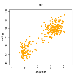
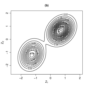
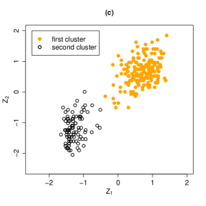
Figure 8.11: (a): Scatterplot of faithful data, (b): contour plot fitted to standardized faithful data, and (c): scatterplot of clustered standardized faithful data.

References

- Andrieu and Atchadé [2006] Christophe Andrieu and Yves F Atchadé. On the efficiency of adaptive mcmc algorithms. In Proceedings of the 1st international conference on Performance evaluation methodolgies and tools, pages 43–es, 2006.
- Arellano-Valle et al. [2007] RB Arellano-Valle, H Bolfarine, and VH Lachos. Bayesian inference for skew-normal linear mixed models. Journal of Applied Statistics, 34(6):663–682, 2007.
- Arellano-Valle and Azzalini [2006] Reinaldo B Arellano-Valle and Adelchi Azzalini. On the unification of families of skew-normal distributions. Scandinavian Journal of Statistics, 33(3):561–574, 2006.
- Arellano-Valle and Genton [2005] Reinaldo B Arellano-Valle and Marc G Genton. On fundamental skew distributions. Journal of Multivariate Analysis, 96(1):93–116, 2005.
- Arfken et al. [2011] George B Arfken, Hans J Weber, and Frank E Harris. Mathematical Methods for Physicists: A Comprehensive Guide. Academic Press, 2011.
- Atchadé and Rosenthal [2005] Yves F Atchadé and Jeffrey S Rosenthal. On adaptive markov chain monte carlo algorithms. Bernoulli, 11(5):815–828, 2005.
- Azzalini [1985] Adelchi Azzalini. A class of distributions which includes the normal ones. Scandinavian Journal of Statistics, pages 171–178, 1985.
- Azzalini and Bowman [1990] Adelchi Azzalini and Adrian W Bowman. A look at some data on the old faithful geyser. Journal of the Royal Statistical Society: Series C (Applied Statistics), 39(3):357–365, 1990.
- Berger et al. [2009] James O Berger, José M Bernardo, and Dongchu Sun. The formal definition of reference priors. The Annals of Statistics, 37(2):905–938, 2009.
- Bernardo [1979] Jose M Bernardo. Reference posterior distributions for bayesian inference. Journal of the Royal Statistical Society Series B: Statistical Methodology, 41(2):113–128, 1979.
- Bernardo [2005] José M Bernardo. Reference analysis. Handbook of Statistics, 25:17–90, 2005.
- Botev [2017] Zdravko I Botev. The normal law under linear restrictions: simulation and estimation via minimax tilting. Journal of the Royal Statistical Society Series B: Statistical Methodology, 79(1):125–148, 2017.
- Box and Tiao [2011] George EP Box and George C Tiao. Bayesian Inference in Statistical Analysis. John Wiley & Sons, 2011.
- Buckle [1995] DJ Buckle. Bayesian inference for stable distributions. Journal of the American Statistical Association, 90(430):605–613, 1995.
- Casella [1985] George Casella. An introduction to empirical bayes data analysis. The American Statistician, 39(2):83–87, 1985.
- Dahlquist and Björck [2003] Germund Dahlquist and Åke Björck. Numerical Methods. Courier Corporation, 2003.
- Dempster et al. [1977] Arthur P Dempster, Nan M Laird, and Donald B Rubin. Maximum likelihood from incomplete data via the em algorithm. Journal of the royal statistical society: series B (methodological), 39(1):1–22, 1977.
- Devroye [1986a] Luc Devroye. Non-uniform random variate generation. 1986a.
- Devroye [1986b] Luc Devroye. Non-Uniform Random Variate Generation. Springer-Verlag, Berlin, Germany, 1986b.
- Devroye [2009] Luc Devroye. Random variate generation for exponentially and polynomially tilted stable distributions. ACM Transactions on Modeling and Computer Simulation (TOMACS), 19(4):1–20, 2009.
- Doob [1949] Joseph L Doob. Application of the theory of martingales. Le calcul des probabilites et ses applications, pages 23–27, 1949.
- Fernández and Steel [1999] Carmen Fernández and Mark FJ Steel. Multivariate student-t regression models: Pitfalls and inference. Biometrika, 86(1):153–167, 1999.