Data-driven rainfall prediction at a regional scale: a case study with Ghana

Abstract

With a warming planet, tropical regions are expected to experience the brunt of climate change, with more intense and more volatile rainfall events. Currently, state-of-the-art numerical weather prediction (NWP) models are known to struggle to produce skillful rainfall forecasts in tropical regions of Africa. There is thus a pressing need for improved rainfall forecasting in these regions. Over the last decade or so, the increased availability of large-scale meteorological datasets and the development of powerful machine learning models have opened up new opportunities for data-driven weather forecasting. Focusing on Ghana in this study, we use these tools to develop two U-Net convolutional neural network (CNN) models, to predict 24h rainfall at 12h and 30h lead-time. The models were trained using data from the ERA5 reanalysis dataset, and the GPM-IMERG dataset. A special attention was paid to interpretability. We developed a novel statistical methodology that allowed us to probe the relative importance of the meteorological variables input in our model, offering useful insights into the factors that drive precipitation in the Ghana region. Empirically, we found that our 12h lead-time model has performances that match, and in some accounts are better than the 18h lead-time forecasts produced by the ECMWF (as available in the TIGGE dataset). We also found that combining our data-driven model with classical NWP further improves forecast accuracy.

Keywords Tropical Rainfall Prediction  $\cdot$ ECMWF Forecast  $\cdot$ Data-Driven forecasting  $\cdot$ Convolutional Neural Ensemble learning  $\cdot$ Feature Importance Estimation

1 Introduction

The precipitation of liquid water from Earth’s atmosphere to the surface is one of the most crucial atmospheric processes shaping life on earth (Box and Box, 2015). Lack of rainfall leads to drought, and too much rainfall often leads to flooding, two natural disasters that have been plaguing human societies since the dawn of time. The spatio-temporal distribution and intensity of precipitation events also hold significant implications for the smooth running of human societies, from day-to-day events, to large-scale urban and agricultural plans. As such, precipitation prediction is an essential tool for planning and decision making. However, rain and other precipitations are notoriously difficult to predict (Tapiador et al., 2019). Unlike most atmospheric variables, rainfall amounts are spatio-temporally non-smooth, and this poses significant challenge to modeling, with many models often based (implicitly or explicitly) on smoothness assumptions.

The situation is particularly problematic under the tropics where rainfall are dominated by multiscale convective flows that are currently challenging to represent in numerical weather prediction (NWP) models (Becker et al. (2021)). In tropical West Africa, this issue is compounded with the lack of quality measurements. As a consequence state-of-the-art NWP models such as the European Center for Mid-Range Weather Forecasting (ECMWF) models are known to struggle to produce skillful forecasts in these regions (Vogel et al. (2020); Kniffka et al. (2020); Rojas-Campos et al. (2023)). At the same time, regions of sub-Sahara Africa are projected to experience the brunt of climate change, with more intense and more volatile precipitation as Earth’s atmosphere warms (WMO, 2024). For instance, flooding from the 2024 raining season in West and Central Africa have claimed the lives of more than a thousand, and displaced close to a million people.

The rise of deep learning (DL) models and the growing availability of extensive weather data sets are ushering in new set of tools and new opportunities for improved weather forecasting (Bouallegue et al. (2024)). Following a similar trend in other areas, several foundation weather forecasting models have recently appeared with striking capabilities (Pathak et al. (2022); Lam et al. (2022); Bi et al. (2023); Chen et al. (2023)). However precipitation remains poorly handled by these foundation AI models, and is often omitted from their evaluations. In some of these models, the approach adopted may not be well-suited for precipitation forecasting. For instance the dynamical system perspective adopted in GraphCast (Lam et al. (2022)) using a mesh-based graph convolutional neural networks is predicated on a smooth dynamics of the atmosphere, which typically does not apply to rainfall under the tropics.

In this work we tackle the tropical rainfall prediction problem at a smaller, region scale. Unlike foundation models, we focus solely on rainfall prediction, and we build models that are more modest in size and can be easily deployed with limited resources. Specifically, using the ERA5 and GPM-IMERG datasets we develop two deep learning (DL) models for 24h rainfall prediction over Ghana, with prediction lead-times of 12 hours and 30 hours respectively. Overall, we found that our 12h lead-time model matches, and in some accounts outperforms the 18h lead-time forecasts by the ECMWF (as available in the TIGGE dataset). Another important contribution of our work is that we develop a statistical method to probe the relative importance of the meteorological variables used in our model, leading to useful insights into the factors driving precipitation in the Ghana region.

Beside foundation models, several other data-driven models have been developed for weather and precipitation prediction at a regional scale (Shi et al., 2015; Dueben and Bauer, 2018; Agrawal et al., 2019; Weyn et al., 2019; Ayzel et al., 2020; Ko et al., 2022; Oh et al., 2023). Several works have also targeted specifically rainfall prediction in West africa using data-driven approaches (Vogel et al. (2020, 2021); Gebremichael et al. (2022); Ageet et al. (2023)), including (Walz et al., 2024a) that uses deep learning techniques and is the closest to our work. Compared to (Walz et al., 2024a), the prediction problem that we consider in this work is more challenging. Indeed, our work focuses on Ghana at a 64-by-64 spatial resolution, compared to a 19-by-61 resolution in (Walz et al., 2024a) for an area 25 times bigger than Ghana. The challenge in rainfall prediction increases significantly as the spatial resolution is refined. Furthermore, we consider predictions with longer lead-times (12h and 30h compared to 6h in (Walz et al., 2024a)). Another important contribution of our work is a novel and widely applicable methodology that has allowed us to assess the relative importance of the meteorological variables used.

The rest of the manuscript is structured as follows. Section 2 presents the general modeling approach and the datasets employed, Section 3 discusses our methodology, specifically the U-Net architecture employed. Section 4 describes the evaluation setup, including a novel approach for probing the importance of the input variables. In Section 5 we present and discuss our finding. Finally Section 6 contains some concluding thoughts.

2 General approach and datasets

The current study focuses on Ghana, a country in West Africa spanning latitudes $4.3^{\circ}$ North to $11.6^{\circ}$ North and longitudes $3.8^{\circ}$ West to $1.8^{\circ}$ East, as depicted on Figure 1. By area size, the country is smaller but comparable to the United Kingdom, and to the state of Michigan in the United States. The climate of Ghana is tropical, with distinct rainy and dry seasons, with the rainy season usually lasting from April to November, followed by a dry season (Manzanas et al., 2014). The rainy season varies with the latitudes: the south typically experiences two rainy seasons (a big rainy season from April to July, and a small one from September to November), whereas the north typically experiences one rainy season from April to October).

Figure 1: Ghana: The area of Interest within West Africa.

For this study daily rainfall measurements and meteorological variables over Ghana were collected from the GPM-IMERG data product developed by the National Aeronautics and Space Administration (NASA), and from the ERA5 data product of the European Center for Mid-range Weather Forecasting (ECMWF). We describe these data products below. Here we give a general overview of our approach. Specifically, our study time-window is June 1st, 2000 to September 30th, 2021, and we discretize the bounding box around Ghana into a $64\times 64$ image. For each date $t$ in the study window, we let ${\bf y}_{t}=\{y_{i,t},\;i\in 64\times 64\}$ be the image of rainfall observations over the 24h of date $t$, obtained from the GPM-IMERG data product. Actually, we follow the convention of GPM-IMERG that defined the 24h rainfall period as 6AM-6AM UTC. Similarly, for each date $t$ in the study window, and for a prediction with lead-time $h$, we collected $K=57$ environmental and meteorological variables over Ghana from the ERA5 data product at time $t-h$, as described below. We denote these variables on pixel $i$ by ${\bf x}_{i,t-h}\in\mathbb{R}^{K}$, and we set ${\bf x}_{t-h}=\{{\bf x}_{i,t-h},\;i\in 64\times 64\}$ for the 3D images of meteorological predictor variables.

For a prediction task with lead-time $h$, we thus obtain a dataset $\mathcal{D}=\{({\bf x}_{t-h},\;{\bf y}_{t}),\;1\leq t\leq T\}$ of size $T=7,791$ that we split into a training set $\mathcal{D}^{\prime}$ and a test set $\mathcal{D}^{{}^{\prime\prime}}$ of size $7736$ ($100$ as validation samples) and $55$, respectively. Using the training set, we train a model that aims to predict ${\bf y}_{t}$ using the variables ${\bf x}_{t-h}$, assuming independent between time points. We explore two lead-time values: $h=12$, and $h=30$. And we evaluate and compare the models using the test set $\mathcal{D}^{{}^{\prime\prime}}$.

2.1 GPM-IMERG precipitation data

The Global Precipitation Measurement (GPM) mission is an international satellite mission launched jointly by NASA and the Japanese JAXA in 2014 for precipitation measurements at the scale of the planet (Hou et al. (2014)). The mission was built on the successful Tropical Rainfall Measuring Mission (TRMM) satellites that operated from 1997 to 2015. The GPM mission carries the first space-borne Ku/Ka-band Dual-frequency Precipitation Radar (DPR) and a multi-channel GPM Microwave Imager (GMI). The Integrated Multi-satellite Retrievals for the Global Precipitation Measurement (IMERG) is a multi-satellite data processing algorithm developed by NASA (Huffman et al. (2020)). The algorithm is applied to the data collected by TRMM and GPM, and further leverages whatever constellation of satellites is available at a given time to produce a long time-series of rainfall measurement at the scale of the planet. The GPM-IMERG product is the current state-of-the-art satellite precipitation observation system, particularly under the tropics. The data is available at a 30-minute temporal resolution and 0.1 degree spatial resolution. For this study, we collected 24h accumulated (6AM-6AM UTC) GPM-IMERG data over the bounding box of Ghana at 0.1 degree spatial resolution, that we then regrid to a $64\times 64$ image. The image obtained for date $t$ is denoted ${\bf y}_{t}$. Although GPM-IMERG is known to have some bias, we will consider it as our precipitation ground truth.

2.2 ERA5 meteorological variables

The ECMWF Reanalysis version 5 (ERA5) is the 5th generation of the gridded reanalysis climate and weather dataset maintained by the European Center for Mid-range Weather Forecasting (ECMWF). See e.g. (Hersbach et al., 2020) for a description. The dataset is produced through reanalysis, that is through a data assimilation approach that combines numerical weather models with global climate observations. ERA5 data contains a large number of environmental and atmospheric variables, from 1940 onwards, at an hour temporal resolution, and $0.25^{\circ}$ spatial resolution. The ERA5 dataset is driving much of the recent machine learning effort for data-driven weather forecasting over the last several years (Keisler (2022); Lam et al. (2022); Chen et al. (2023)). We note that the dataset is not available in real-time. Its current latency is 5 days. This means that our model – like most other data-driven weather prediction models that rely on ERA5 data as inputs – is not currently operationally implementable.

Table 1 lists the 55 ERA5 variables used for this project. We compiled this list from the literature, notably Walz et al. (2024a), as well as from a basic correlation analysis. We group the variables following Walz et al. (2024a). As noted in Walz et al. (2024a), all these variables have been reported in the literature as playing some role in rain formation processes. We retrieved these variables over the bounding box around the Ghana region: $(3.8^{\circ}W,1.8^{\circ}E)$, and $(11.6^{\circ}N,4.3^{\circ}S)$, and with a temporal resolution of six hours.

Table 1: ERA5 variables collected

Variable	Name	Levels (in hPa)
Specific rainwater content	crwc	850, 925, 950
Total column water vapor	tcwv	single level
Total cloud cover	tcc	single level
Total column liquid water	tclw	single level
Vertic. integ. moist. div.	vimd	single level
K index	kx	single level
Convec. avail. pot. energy	cape	single level
Convective inhibition	cin	single level
Surface pressure	sp	single level
Surface temperature	t2m	single level (2m)
Dewpoint temperature	d2m	single level (2m)
Relative humidity	r	300, 500, 600, 700, 850, 925, 950
Specific humidity	q	300, 500, 600, 700, 850, 925, 950
Temperature	t	300, 500, 600, 700, 850, 925, 950
Components of wind	u, v, w	300, 500, 600, 700, 850, 925, 950

Since Ghana has a seasonal rainfall pattern that also varies strongly with latitude, accounting for space-time variability in the model is crucial for accurate forecasts. Thus in addition to the 55 variables listed in Table 1, for each pixel $i$ and each date $t$, we also constructed two new variables

$$\textsf{COS}_{i,t}=\cos\left(2\pi\frac{\mathsf{day}(t)}{365}\right)\times\mathsf{lat}(i),$$ (1)

$$\textsf{SIN}_{i,t}=\sin\left(2\pi\frac{\mathsf{day}(t)}{365}\right)\times\mathsf{lat}(i),$$ (2)

where $\mathsf{day}(t)\in\{1,\ldots,365\}$ is the day of the year of date $t$, and $\mathsf{lat}(i)$ is the latitude of the center point of pixel $i$.

In summary, for each date $t$ in our study window (between June 1st, 2000 and September 30th, 2021), and for each pixel $i\in 64\times 64$, we collected ${\bf x}_{i,t-h}\in\mathbb{R}^{57}$, composed of the values of the 55 variables listed in Table 1, plus the two constructed variables $\mathsf{COS}$ and $\mathsf{SIN}$, $h$ hours before 6AM UTC of date $t$.

2.3 TIGGE forecast data

We compare the skills of our models with the predictions from the European Center for Mid-range Weather Forecasting (ECMWF) made available through the THORPEX Interactive Grand worldwide Ensemble (TIGGE) program (Swinbank et al. (2016)). The TIGGE database has established itself as a key window into the capability of state-of-the-art operational NWP models, and has proven very useful to the research community. For this project we use the Noon-forecasts of the ECMWF model, which corresponds to a 18h lead-time 24h rainfall forecast. The ECMWF forecast that would match our 12h lead-time is not available in TIGGE. We downloaded their total rainfall (the sum of large scale organized precipitation and convective precipitation), that we re-grid to $64\times 64$ images.

3 Methodology

We relate the rainfall image observation ${\bf y}_{t}$ to the environmental and meteorological variables ${\bf x}_{t-h}$ via the model

$${\bf y}_{t}=\mathcal{F}_{W}\left({\bf x}_{t-h}\right)+\bm{\epsilon}_{t},\;\;\;t=1,\ldots,T,$$ (3)

for some error term $\bm{\epsilon}_{t}$. We assume that the error terms $\{\bm{\epsilon}_{t},\;1\leq t\leq T\}$ are independent and identically distributed. This is clearly a strong assumption, and it may be possible to improve the model by leveraging temporal dependence in the data. We leave this issue for further research. For constructing the function $\mathcal{F}_{W}$, we employ a U-Net architecture with weight parameter $W$ (Ronneberger et al., 2015). The U-Net is a CNN-based deep neural network (DNN) architecture specifically designed for image tasks. In contrast to more computationally expensive architectures like graph neural networks (GNNs) and Transformers, U-Net models offer a balance between accuracy and efficiency. It leverages a unique encoder-decoder structure with skip connections to achieve high segmentation accuracy while maintaining computational efficiency. Specifically, we utilize a 2D U-Net model with three downsampling blocks, each containing two convolutional layers, followed by three upsampling blocks with skip connection (see Figure 2).

Figure 2: The U-Net architecture employed. In each block, the first dimension indicates the number of feature maps, while the second and third dimensions correspond to the width and height of each feature map. The input dimensions consist of 57 (representing weather variables), followed by a width of 64 and a height of 64, respectively.

Using the same U-Net architecture, we trained two models with different lead-times. The first model has a lead-time $h=12$ hour that we denote by $\mathsf{UNET}_{12}$ (this model uses as input, the state of the meteorological variable at 6PM, 12 hours before the 6AM-6AM rainfall window). The second model has a lead-time of $h=30$ hour, and is denoted $\mathsf{UNET}_{30}$ (based on meteorological variables at Midnight, 30 hours before the 6AM-6AM rainfall window).

Given the training data $\mathcal{D}^{\prime}$, we train the U-Net models (3) by minimizing the L1 loss

$$\textsf{L}(W;\mathcal{D})=\sum_{t\in\mathcal{D}^{\prime}}\;\left\|\textbf{y}_{t}-\mathcal{F}_{W}\left({\bf x}_{t-h}\right)\right\|_{1},$$ (4)

where for an image ${\bf a}$, $\|{\bf a}\|_{1}$ denotes the sum of the absolute values of the pixel values of ${\bf a}$. The L1 loss is used for added robustness to outliers. We solve this minimization problem using the Adam optimizer (Kingma and Ba (2015)) with a learning rate of $1e^{-4}$ and a weight decay of $1e^{-4}$. During training, a batch size of $256$ is used (based on the availability of the GPU memory). We adjust the learning rate dynamically during training, using the ReduceLROnPlateau method Krizhevsky et al. (2012). This scheduler monitors the loss and adjusts the learning rate when a plateau in performance is detected. Specifically, the learning rate is reduced by a factor of $0.1$ if no improvement is observed in the loss for a specified patience period of $100$ epochs.

If $\widehat{W}$ is an approximate solution to the minimization of (4), and given a new test data point ${\bf x}_{t^{\prime}-h}\in\mathcal{D}^{{}^{\prime\prime}}$, we predict the rainfall amount at time $t^{\prime}$ using

$$\hat{\bf y}_{t^{\prime}}=\mathcal{F}_{\widehat{W}}\left({\bf x}_{t^{\prime}-h}\right).$$

We evaluate the performance of the model by comparing $\hat{\bf y}_{t^{\prime}}$ and ${\bf y}_{t^{\prime}}$ over the test set $\mathcal{D}^{{}^{\prime\prime}}$, as we describe below.

3.1 Combining $\mathsf{UNET}_{12}$ and ECMWF forecasts

In addition of the two models $\mathsf{UNET}_{12}$ and $\mathsf{UNET}_{30}$ we also explore a prediction model that combines $\mathsf{UNET}_{12}$ with the 18h lead-time forecast of the ECMWF obtained from the Tigge database. This averaging approach takes stock in the distinctive features of both methodologies, potentially yielding a more accurate forecast. To accomplish this, and after some trial-and-errors, a weighted average of the ECMWF forecast (with weight $0.1$), and the $\mathsf{UNET}_{12}$ prediction (with weight $0.9$) is proposed. The resulting ensemble weighted average forecast will be denoted below by $\mathsf{Ens}$.

4 Model evaluation

We evaluate and compare four models: $\mathsf{UNET}_{12}$, $\mathsf{UNET}_{30}$, the 18h lead-time predictions of the ECMWF obtained from TIGGE, and denoted as $\mathsf{NWP}$, and model $\mathsf{Ens}$ that is the weighted average of $\mathsf{UNET}_{12}$ and $\mathsf{NWP}$. We use the climatology prediction as reference, and denote it as $\mathsf{CLIM}$. The climatology rainfall prediction at location $i$ and date $t$ is defined as the average of all the 24h rainfall values in the GPM-IMERG data set occurring at location $i$, and on same day of the year as $t$ (plus two days prior and two days after). We compare these models using the mean absolute error (MAE), as well as the precision, recall and F1-score for rainfall event detection.

4.1 Prediction error

For a given model $m\in\{\mathsf{CLIM},\mathsf{UNET}_{12},\mathsf{UNET}_{30},\mathsf{NWP},\mathsf{Ens}\}$, we write $\hat{y}_{it^{\prime}}(m)$ to denote the predicted rainfall at location $i\in 64\times 64$, and at time $t^{\prime}$ by model $m$. The mean absolute prediction error (MAE) of model $m$ at pixel $i$ is defined as

$$\ell(i,m)=\frac{1}{|\mathcal{D}^{{}^{\prime\prime}}|}\sum_{t^{\prime}\in\mathcal{D}^{{}^{\prime\prime}}}\left|\widehat{y}_{i,t^{\prime}}(m)-y_{i,t^{\prime}}\right|,$$

where the average is taken over the test dataset $\mathcal{D}^{{}^{\prime\prime}}$. This metric can also be viewed as a special case of the CRPS (Gneiting and Raftery (2007)) with one forecast value. Using the NWP prediction as reference, we compute the pixel-by-pixel prediction error skill of model $m$ as

$$\mathsf{Skill}(i,m)=\frac{\ell(i,\mathsf{NWP})-\ell(i,m)}{\ell(i,\mathsf{NWP})},$$ (5)

which offers a visual evaluation of model $m$. As defined, $\mathsf{Skill}(i,m)$ is positive if model $m$ performs better than the ECMWF forcast at $i$, and $\mathsf{Skill}(i,m)$ is nonpositive otherwise.

4.2 Precision, recall, and F1-score

We also compare the models in their ability to correctly predict rainfall events. Given a threshold level $\tau$, and a model $m\in\{\mathsf{CLIM},\mathsf{UNET}_{12},\mathsf{UNET}_{30},\mathsf{NWP},\mathsf{Ens}\}$, its precision and recall at pixel $i$ are defined respectively as

$$\mathcal{P}_{i}(m)=\frac{\sum_{t^{\prime}\in\mathcal{D}^{{}^{\prime\prime}}}\textbf{1}_{\left\{|\hat{y}_{it^{\prime}}|>\tau\right\}}\textbf{1}_{\left\{|y_{it^{\prime}}|>\tau\right\}}}{\sum_{t^{\prime}\in\mathcal{D}^{{}^{\prime\prime}}}\textbf{1}_{\{|\hat{y}_{it^{\prime}}|>\tau\}}},\;\;\mathcal{R}_{i}(m)=\frac{\sum_{t^{\prime}\in\mathcal{D}^{{}^{\prime\prime}}}\textbf{1}_{\{|\hat{y}_{it^{\prime}}|>\tau\}}\textbf{1}_{\{|y_{it^{\prime}}|>\tau\}}}{\sum_{t^{\prime}\in\mathcal{D}^{{}^{\prime\prime}}}\textbf{1}_{\{|y_{it^{\prime}}|>\tau\}}}.$$

We further combine the precision and the recall into a $(\mathcal{F}_{1})$ score

$$(\mathcal{F}_{1})_{i}(m)=\frac{2\mathcal{P}_{i}(m)\mathcal{R}_{i}(m)}{\mathcal{P}_{i}(m)+\mathcal{R}_{i}(m)}.$$

We further average the precision statistic $\mathcal{P}_{i}(m)$ across pixels to obtain the overall precision of model $m$ as

$$\mathcal{P}(m)=\frac{1}{4096}\sum_{i}\mathcal{P}_{i}(m).$$

We compute $\mathcal{R}(m)$ and $(\mathcal{F}_{1})(m)$ similarly. We compute these statistics with two threshold values: $\tau=0.5$mm which allows us to compare the models in their ability to predict rainfall events, and $\tau=10$mm to evaluate the ability of the models to prediction heavy rainfall events (a larger value of $\tau$ would lead to rare-events and high-variance estimates).

4.3 Probing the importance of the input variables

One of the main limitations of deep learning models is their lack of interpretability. With the development and adoption of these techniques in Earth science research, there is a growing need for interpretable/explanable deep learning models (Bommer et al., 2024). We focus here on our model $\mathsf{UNET}_{12}$, and we propose a novel methodology to evaluate the importance of its input predictors. Let $\mathcal{F}_{\hat{W}}$ denote the fitted model $\mathsf{UNET}_{12}$. We recall that the input feature ${\bf x}$ is of dimension ${\bf x}\in\mathbb{R}^{K\times I}$, where $K$ denote the number of variables, and $I$ the number of pixels (we have collapsed the longitude and latitude dimensions into one pixel dimension). One common approach that one could use to measure the importance of a given feature input in this setting is the sensitivity of the predicted rainfall with respect to that input (Baehrens et al., 2010; Bommer et al., 2024). Specifically, the sensitivity of the predicted rainfall to the input variable $k$ is defined as

$$\frac{1}{|\mathcal{D}^{{}^{\prime\prime}}|}\sum_{t^{\prime}\in\mathcal{D}^{{}^{\prime\prime}}}\;\sum_{\iota}\;\left|{\bf s}_{k,\iota}({\bf x}_{t^{\prime}})\right|,\;\;\mbox{ where }\;\;{\bf s}_{k,\iota}({\bf x})=\frac{1}{2}\frac{\partial\|\mathcal{F}_{\hat{W}}({\bf x})\|_{2}^{2}}{\partial{\bf x}_{k,\iota}},$$

where the average is over the test dataset $\mathcal{D}^{{}^{\prime\prime}}$. (Bommer et al., 2024) presented several variations of this metric that have been used in the literature. We note however that these sensitivity metrics are defined without any reference to model performance. Hence a variable could have high sensitivity without being essential for accurate prediction.

To address this issue, we propose a novel methodology built on the idea of posterior predictive checking, a powerful tool in Bayesian data analysis for model checking and validation (Gelman et al. (2004)). The basic idea is the use of the posterior predictive distribution as a data generating process for the test data. Based on that data generating process we then perform a variable selection to determine which input variable best explains the observed performance on the test data. To be more specific, suppose for a moment that we have fitted our deep neural network model in the Bayesian framework with a posterior distribution $\Pi(\cdot|\mathcal{D}^{\prime})$. Then the posterior predictive distribution of a data point $\mathbf{x}_{t-h}$ in the test set $\mathcal{D}^{{}^{\prime\prime}}$ would be defined as

$$\hat{f}(\mathbf{x}_{t-h})=\int\exp\left(-\frac{1}{2\sigma^{2}}\|\mathbf{y}_{t}-\mathcal{F}_{W}(\mathbf{x}_{t-h})\|_{1}\right)\Pi(W|\mathcal{D}^{\prime})\mathrm{d}W.$$

To the $K=57$ input variables in model (3), we assign binary variables $\delta=(\delta_{1},\ldots,\delta_{K})$, where $\delta_{k}\in\{0,1\}$. Let $\delta\odot\mathbf{x}_{t}$ be the input data point with the same size as $\mathbf{x}_{t}$, but where the channel of the $j$-th variable is multiplied by $\delta_{j}$. In other words, with $\delta\odot\mathbf{x}_{t}$, we mask out from the input data, all the variables $j$ for which $\delta_{j}=0$. We endow each $\delta_{j}$ with a Bernoulli prior distribution: $\delta_{j}\sim\textbf{Ber}(1/(1+e^{r}))$, for some hyper-parameter $r$ to be set by the user. Note that under this prior distribution, the probability $\mathbb{P}(\delta_{k}=1)$ is of order $e^{-r}$, and thus can be very small even for $r$ modestly large. Given this prior distribution and the posterior predictive model, we consider the posterior distribution (from the posterior predictive model)

$$\Pi(\delta_{1},\ldots,\delta_{K}|\mathcal{D}^{\prime}\cup\mathcal{D}^{{}^{\prime\prime}})\propto\exp\left(-r\sum_{j=1}^{K}\delta_{j}\right)\;\prod_{t\in\mathcal{D}^{{}^{\prime\prime}}}\;\hat{f}(\delta\odot\mathbf{x}_{t-h}),$$ (6)

which gives the relative importance of each variable $\delta_{j}$ in explaining the performance of our fitted model $\Pi(W|\mathcal{D}^{\prime})$ on the test data $\mathcal{D}^{{}^{\prime\prime}}$. We note that the posterior predictive distribution $\Pi(\delta|\mathcal{D}^{\prime}\cup\mathcal{D}^{{}^{\prime\prime}})$ in (6) depends both on the test set $\mathcal{D}{{}^{\prime\prime}}$ and the training set $\mathcal{D}^{\prime}$. We note also that the test set $\mathcal{D}^{{}^{\prime\prime}}$ is typically not very large, therefore we do not expect $\Pi(\delta|\mathcal{D}^{\prime}\cup\mathcal{D}^{{}^{\prime\prime}})$ to concentrate, in the sense of putting high probability on a small number of variables. Instead it provides a ranking of the relative importance of the input variables in explaining the performance of the fitted model on the test data.

Now, since we did not build our deep learning model in the Bayesian framework, the implementation of the procedure outlined above needs some adjustments. Specifically, we will replace the posterior distribution $\Pi(W|\mathcal{D}^{\prime})$ by a point mass measure at $\hat{W}$, where $\hat{W}$ is the minimizer of (4) obtained above from the training dataset $\mathcal{D}^{\prime}$. The resulting approximation to the posterior distribution (6) is

$$\Pi\left(\delta_{1},\ldots,\delta_{K}|\mathcal{D}^{\prime}\cup\mathcal{D}^{{}^{\prime\prime}}\right)\propto\exp\left(-r\sum_{j=1}^{K}\delta_{j}-\frac{1}{2\sigma^{2}}\mathsf{L}(\delta;\mathcal{D})\right),$$ (7)

where

$$\textsf{L}(\delta;\mathcal{D})=\sum_{t\in\mathcal{D}^{{}^{\prime\prime}}}\left\|\textbf{y}_{t}-\mathcal{F}_{\widehat{W}}(\delta\odot\mathbf{x}_{t-h})\right\|_{1}.$$

We note that L depends both on the test set $\mathcal{D}{{}^{\prime\prime}}$ and the training set $\mathcal{D}^{\prime}$. We sample from (7) using a straightforward Gibbs sampling. For an introduction to MCMC and the Gibbs sampler, we refer the reader to (Brooks et al., 2011). Specifically, given $\delta\in\{0,1\}^{K}$, and $1\leq j\leq K$, let $\delta^{(j,1)}$ (resp. $\delta^{(j,0)}$) be the element of $\{0,1\}^{K}$, that is equal to $\delta$ except perhaps on component $j$, where $(\delta^{(j,1)})_{j}=1$ (resp. $(\delta^{(j,0)})_{j}=0$). Then under the joint (7), the conditional distribution of $\delta_{j}$ given the remaining components denoted $\delta_{-j}$ and given $\mathcal{D}$ is a Bernoulli distribution $\textbf{Ber}(q_{j})$, with probability $q_{j}$ given by

$$q_{j}=\left[1+\exp\left\{r+\frac{1}{2\sigma^{2}}\left(\mathsf{L}(\delta^{(j,1)};\mathcal{D})-\mathsf{L}(\delta^{(j,0)};\mathcal{D})\right)\right\}\right]^{-1}.$$

$q_{j}$ can be computed at the cost of two forward runs through the model $\mathcal{F}_{\hat{W}}$ using the test data sets with masks $\delta^{(j,0)}$ and $\delta^{(j,1)}$ applied.

5 Results and Discussion

We evaluate the performance of the models using the metrics presented above. As a start, Figure 3 shows some prediction samples from the models.

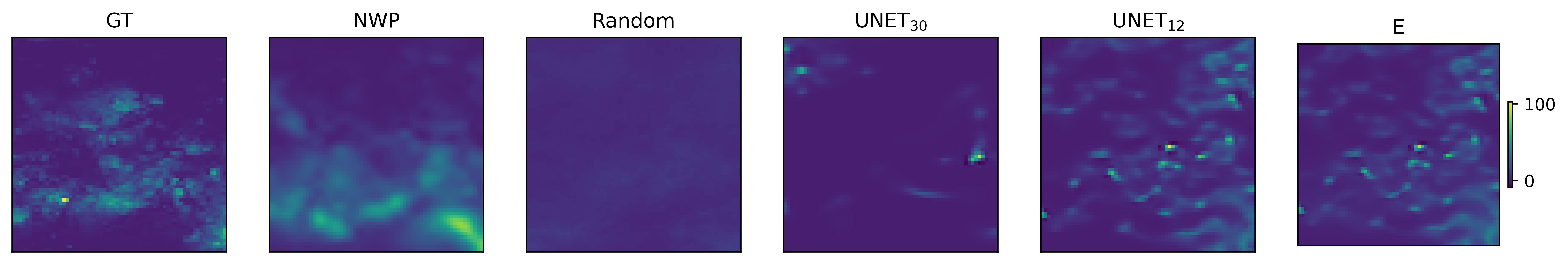
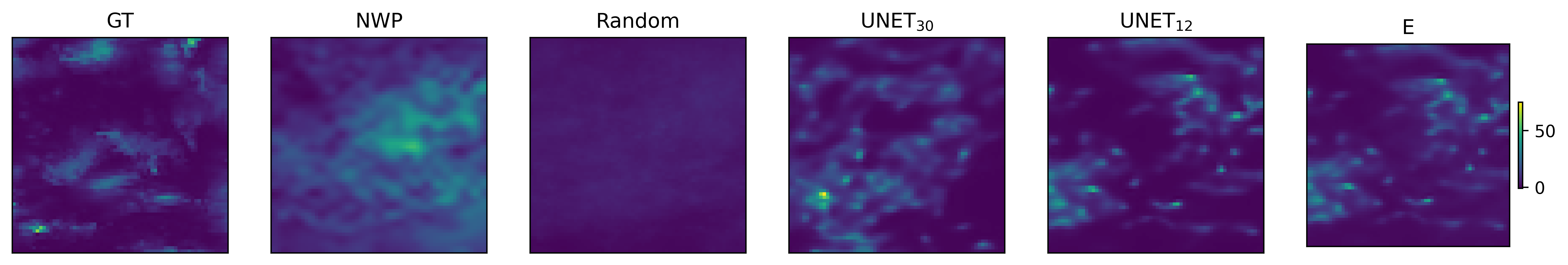
Figure 3: Sample forecasts ($\mathsf{NWP}$, $\mathsf{CLIM}$, $\mathsf{UNET}_{30}$, $\mathsf{UNET}_{12}$, and $\mathsf{Ens}$), along with the corresponding ground truth (GT) from GPM-IMERG.

5.1 Comparison in terms of mean absolute error

Table 2 shows the overall mean and standard deviation of the mean absolute errors computed across all pixels in the test dataset. The results show that in terms of the mean absolute error, the numerical weather prediction model $\mathsf{NWP}$ model is comparable to the climatology $\mathsf{CLIM}$, but $\mathsf{UNET_{12}}$ and the ensemble model show clear improvement. The fact that the numerical weather prediction model does not outperform the climatology forecast under the tropics is well-documented as we discussed in the introduction (Vogel et al. (2020)). However, climatology forecasts are broad averages and therefore lack precision as we will see below.

Figure 4 shows the MAE skill maps of the models compared to $\mathsf{NWP}$ as given in (5). White areas holds negative values and indicate locations at which the NWP has better MAE. The maps show the NWP significantly under-performs $\mathsf{UNET_{12}}$, Ens, (and $\mathsf{UNET_{30}}$ to a lesser extent), particularly in the coastal south and the north.

Table 2: Means and standard deviations of the Mean absolute errors

	CLIM	NWP	$\mathsf{UNET}_{30}$	$\mathsf{UNET}_{12}$	Ens
Mean	3.89	3.92	3.83	3.74	3.63
Std	1.15	1.12	1.28	1.13	1.10

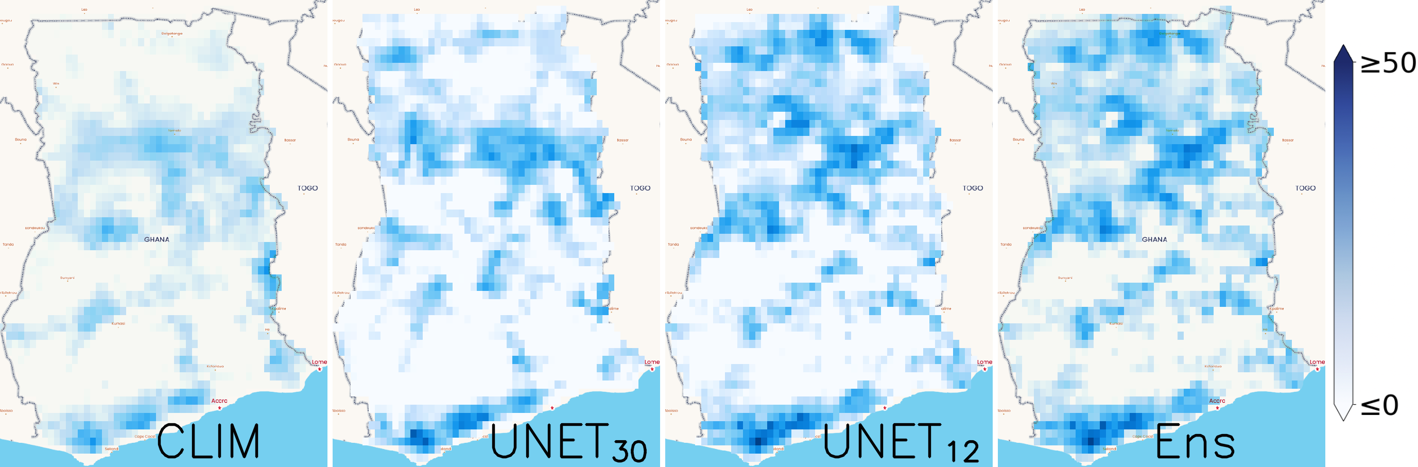
Figure 4: MAE skill maps. We treat the spatial locations as independent. Each skill value is computed as in (5)

5.2 Comparing the biases of $\mathsf{NWP}$ and $\mathsf{UNET}_{12}$ predictions

Here we further investigate the structure of the prediction biases of the models $\mathsf{NWP}$ and $\mathsf{UNET}_{12}$. We combine all the pixels of all the test samples together, and look at the proportion of pixels with bias (defined as the difference between the predicted rainfall and the corresponding GPM-IMERG estimate) falling within each of the following ranges $(-0.1,0)$, $(0,0.1)$, $(-1,0)$, and $(0,-1)$. The results are presented in Table 3. We note that $\mathsf{UNET}_{12}$ has 50% more bias values in the interval $(-0.1,0.1)$ than $\mathsf{NWP}$, and 22% more bias values in the interval $(-1,1)$. These statistics support again our conclusion that the DL model $\mathsf{UNET}_{12}$ performs better than $\mathsf{NWP}$. We note however that $\mathsf{UNET}_{12}$ has a strong tendency to underestimate the rainfall values, whereas $\mathsf{NWP}$ has a tendency to overestimate the rainfall values. These observed bias patterns has motivated the introduction of our ensemble forecast model Ens that combines $\mathsf{UNET}_{12}$ and $\mathsf{NWP}$.

Table 3: Proportion of pixels (in percentage) in each range

Model	Proportions
	(-0.1, 0)	(0, 0.1)	(-1, 0)	(0, 1)
$\mathsf{NWP}$	11.99	16.72	16.39	32.74
$\mathsf{UNET}_{12}$	34.07	10.00	42.26	17.69

5.3 Comparison in terms of precision and recall

Correctly matching the tail events of the rainfall distribution has significant practical values. Here we compare our forecast models in their ability to correctly predict rainy days and heavy rainy days (days with 24h rainfall larger than $0.5$mm, and $10$mm respectively). Using the GPM-IMERG as ground truth, we compare the models in terms of precision (P), recall (R) and F1 score as described in Section 4. Table 4 summarizes the overall performance of each model. We first consider the detection of rainy days (at threshold $\tau=0.5$mm). As expected, due to broad averaging, the CLIM forecast suffers from low precision ($0.45$), as it frequently misclassifies non-rain events as rain. Similarly, the NWP model also shows a strong recall ($88\%$) but a relatively low precision ($0.52$). This suggests that the NWP model captures much of the rainfall signal, but also has some amount of spurious phenomena driving its forecasts. In contrast, the data-driven models have lower recall, which suggests that these models are missing some of the rainfall signal (the physics), however they have better precision. The ensemble model (Ens) is able to leverage the complementary strengths of the two approaches and scores better. The location-wise distribution of P and R across the area of interest can be further visualized in Figures 5 and 6, respectively.

Table 4: The overall Precision (P), Recall (R), and F1-Score (F1) of the models at the threshold, $\tau=0.5$ and $10$

Model	$\tau=0.5$			$\tau=10$
	Precision	Recall	F1	Precision	Recall	F1
$\mathsf{CLIM}$	0.45	0.97	0.61	0.17	0.02	0.04
$\mathsf{NWP}$	0.52	0.88	0.65	0.27	0.25	0.26
$\mathsf{UNET}_{30}$	0.59	0.57	0.58	0.23	0.14	0.17
$\mathsf{UNET}_{12}$	0.62	0.64	0.63	0.31	0.26	0.28
$\mathsf{Ens}$	0.61	0.79	0.69	0.32	0.25	0.28

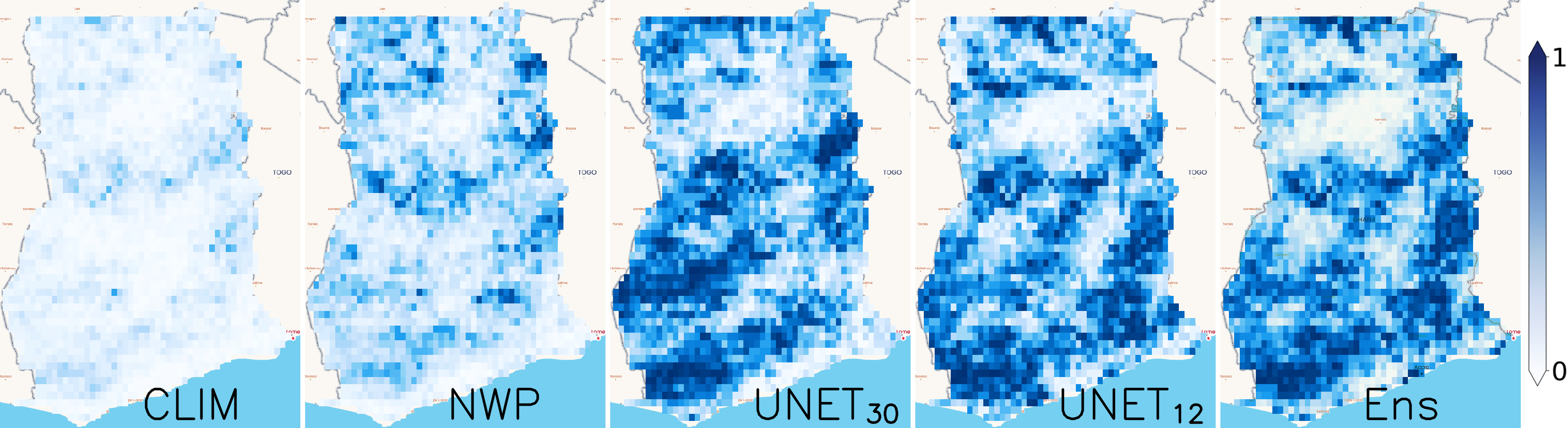
Figure 5: Locationwise precision (P) of the models at threshold $\tau=0.5$mm

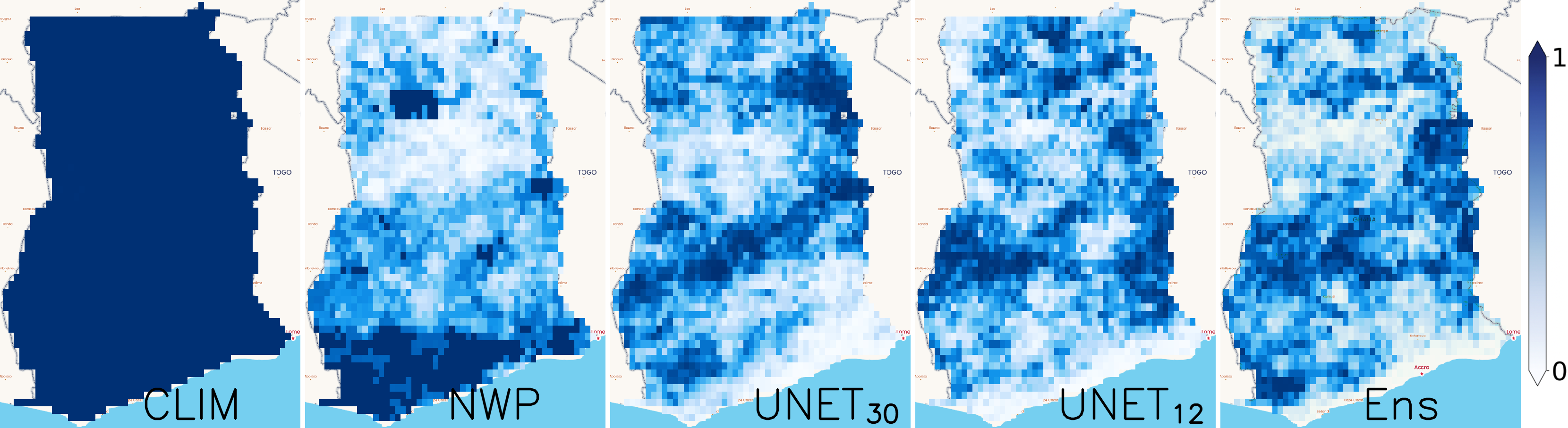
Figure 6: Locationwise recall (R) of the models at threshold $\tau=0.5$mm

5.3.1 Detection of heavy rainfall

We also compare the models through their predictions of heavy rainy days, particularly on how such predictions agree with GPM-IMERG. We set the threshold for heavy rain to $\tau=10$mm. The performance of the models is much worst. This suggests that more work is needed to better predict large and extreme rainfall events. Figures 7 and 8 show the location-wise distribution of P and R across the area of interest (AOI). From these figures we see again that $\mathsf{UNET_{12}}$ (and $\mathsf{UNET_{30}}$ to a lesser extent) performs better than NWP.

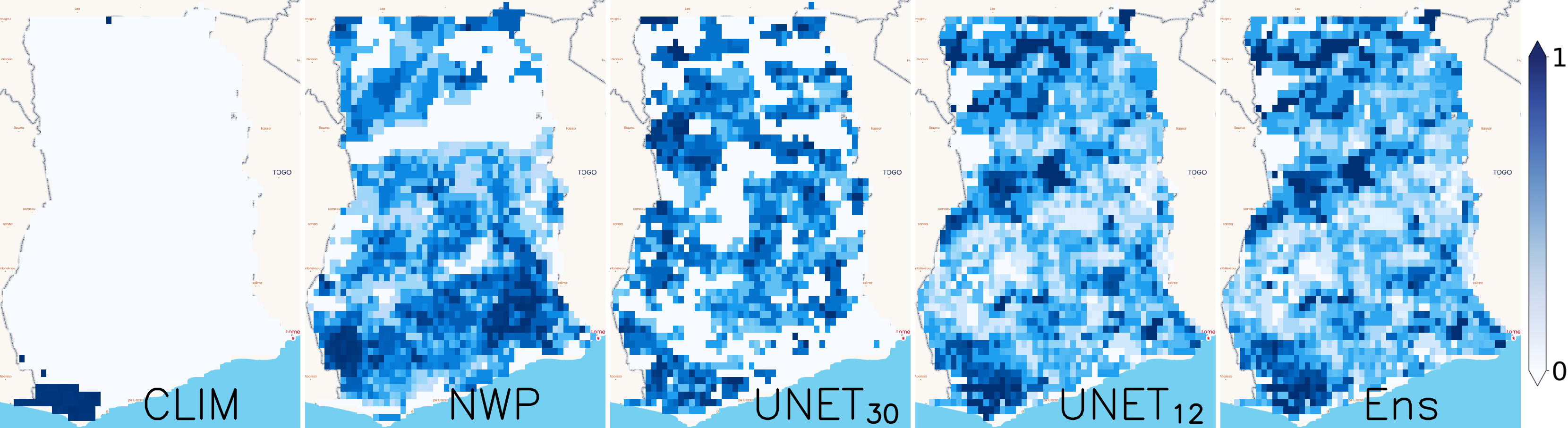
Figure 7: Locationwise precision (P) of the models at threshold $\tau=10$mm

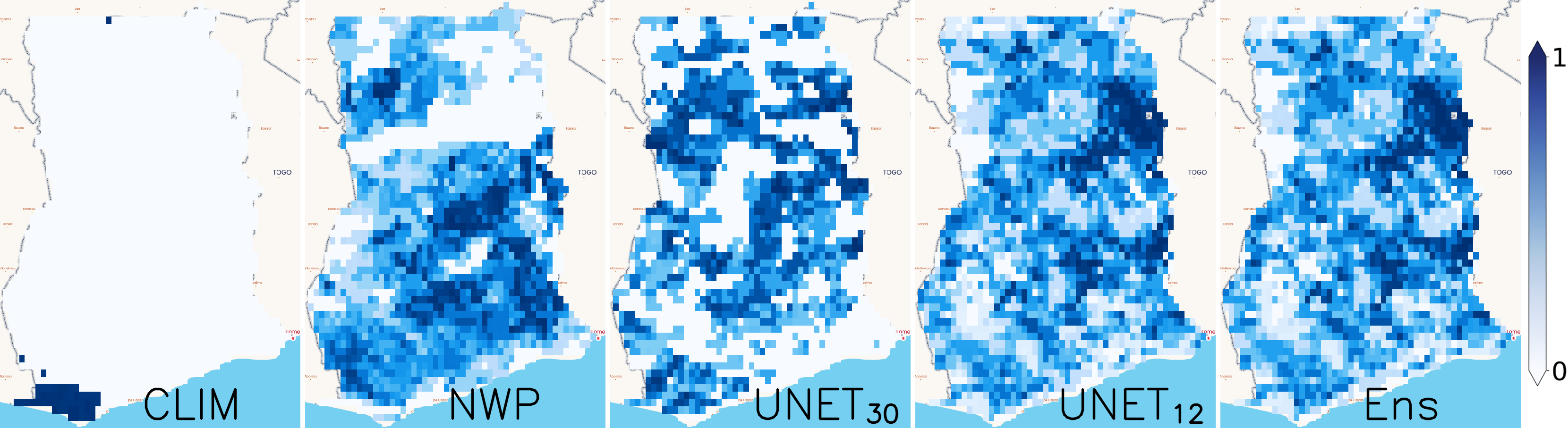
Figure 8: Locationwise recall (R) of the models at threshold $\tau=10$mm

5.4 Input variables selection

We run the Gibbs sampler described in Section 4.3 for $1,000$ epochs, where each iteration is a full sweep through the $K$ variables. We use $\sigma^{2}=0.01$, and $r=3.76$. We discard the first 950 epochs as burn-in. For each input variable $j$, we take the average of $\delta_{j}$ along the MCMC output as an estimate of the posterior probability of $\delta_{j}$. Figure 9 shows the $30$ largest posterior probabilities. The results show that the most important predictive variable is the spatio-temporal variable Cos defined in (1). This is hardly surprising since rainfall in Ghana is known to have a strong seasonality which varies with latitude. Evaporation drives rainfall, and our method indeed highlights specific humidity ($q925$), relative humidity ($r950$) and total column water vapor ($tcwv$) as important input variables. The variable wind ($u300$) also appears important. The wind variable $u300$ is possibly related to the African Easterly Jet (AEJ), which plays a fundamental in the West African monsoon. However, additional research is needed on this connection, since the bulk of the AEJ is typically located much lower, at around $700$hPa. Our methodology also highlights several convection-related variables: convective inhibition ($cin$), K-index ($kx$) and the convective available potential energy ($cape$) as key input variables. This is consistent, since a large part of the rainfall in Ghana is convection-driven. One important limitation of our methodology is that it does not offer much insight on the physical process(es) by which these variables affect rainfall. More research is needed on this point.

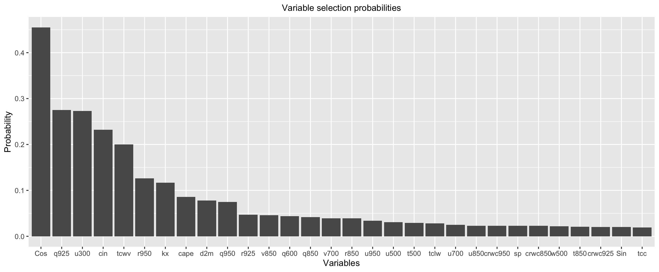
Figure 9: Top 30 marginal posterior means of input variables using samples from the posterior distribution (7).

6 Conclusion

This research dealt with the challenging problem of predicting rainfall in tropical regions. Although we have focused on Ghana, our methodology can be readily applied to other regions. Our proposed data-driven model is a U-Net convolutional neural network model (CNN) that we trained to predict 24h rainfall at 12h and 30h lead-time using data from ERA5 and GPM-IMERG. As illustrated, the 12h lead-time prediction model shows significant improvement over a numerical weather prediction (NWP) model developed by the ECMWF as obtained through TIGGE. Our investigation also found that a strategy that mixes our U-Net model and NWP further enhanced forecasting performance. We also developed a novel methodology that enhanced the interpretability of our model, by identifying the input variables that best capture the performance of the model.

Our work comes with several limitations, but also opens up several avenues for further research that we hope to tackle in the future. Although we have identified a small list of variables that appear to play an important role in the forecasts, the precise physical processes by which these variables impact rainfall remain largely unclear. There is a growing literature that combines statistics, machine learning and partial differential equations and aims to discover new physical laws from data (Raissi et al., 2019; Chen et al., 2020). Extending these methods to atmospheric sciences can provide a powerful empirical framework to identifying the physical processes involved in the present study.

Another major limitation of our work is the lack of probabilistic forecast and uncertainty quantification (UQ). Fully addressing this issue in a way that captures correctly both the aleatoric and epistemic uncertainties requires further methodological advances than what is currently available in the literature. We refer the reader to (Haynes et al., 2023) for a good review and illustration of the current state-of-the-art on UQ in environmental sciences. Clearly, some degree of uncertainty quantity can be easily achieved by training an ensemble of our U-Net models. However, the practical reliability of these methods remains limited. Particularly, it is unclear whether these methods can reliably capture the aleatoric uncertainty (see Haynes et al. (2023) for further discussion). Another interesting methodology for UQ from single model outputs is the EasyUQ of (Walz et al., 2024b). However, although very easy to implement, the methodology relies on a fundamental monotonicity assumption that in general is untestable. There is a burgeoning literature that aims to develop rigorous Bayesian methodology for training deep learning models (Wilson and Izmailov, 2020; Atchade and Wang, 2023), with suitable built-in UQ. However the implementation cost of these algorithms for the moment seems prohibitive. Overall, given the state of the literature, and despite the fundamental importance of UQ in predictive modeling, we have chosen to defer this issue to future research.

Another notable shortcoming of our method is its poor performance in predicting heavy and extreme rainfall events, driven mainly by the lack of sufficient tail event data. Models for better prediction of tail-events in statistics are often built using quantile regression. However, quantile regression at extreme quantile levels suffer from the same lack of tail data as in this study. New methodology are thus needed to address this issue, perhaps along the emerging literature of extreme quantile regression that merges classical quantile regression and extreme value theory (Velthoen et al. (2023); Pasche and Engelke (2024)).

Finally, we acknowledge that, due to the current 5-days latency on the ERA5 dataset, our forecast models are currently not operational. This delay in data availability, (which affects all models, including foundation models built on ERA5) clearly creates a barrier to the widespread deployment of data-driven weather forecasting.

Data and Code Availability

This research was conducted entirely from publicly available data for research purpose. The code to process the data and train our models are available at the Github address https://github.com/indrakalita/RainfallForecasting. The address also includes a script that utilizes the cdsapi interface to download the ERA5 data. We have used the website interface https://gpm.nasa.gov/data/directory and (https://apps.ecmwf.int/datasets/data/tigge/levtype=sfc/type=cf/ to download the GPM-IMERG and TIGGE data, respectively.

References

- Box and Box [2015] Michael A Box and Gail P Box. Physics of radiation and climate. Taylor and Francis, 2015. ISBN 9781466572058.
- Tapiador et al. [2019] Francisco J. Tapiador, Rémy Roca, Anthony Del Genio, Boris Dewitte, Walt Petersen, and Fuqing Zhang. Is precipitation a good metric for model performance? Bulletin of the American Meteorological Society, 100(2):223 – 233, 2019. doi:10.1175/BAMS-D-17-0218.1.
- Becker et al. [2021] Tobias Becker, Peter Bechtold, and Irina Sandu. Characteristics of convective precipitation over tropical africa in storm-resolving global simulations. Quarterly Journal of the Royal Meteorological Society, 147(741):4388–4407, 2021. doi:https://doi.org/10.1002/qj.4185.
- Vogel et al. [2020] Peter Vogel, Peter Knippertz, Andreas H. Fink, Andreas Schlueter, and Tilmann Gneiting. Skill of global raw and postprocessed ensemble predictions of rainfall in the tropics. Weather and Forecasting, 35(6):2367 – 2385, 2020.
- Kniffka et al. [2020] Anke Kniffka, Peter Knippertz, Andreas H. Fink, Angela Benedetti, Malcolm E. Brooks, Peter G. Hill, Marlon Maranan, Gregor Pante, and Bernhard Vogel. An evaluation of operational and research weather forecasts for southern west africa using observations from the dacciwa field campaign in june-july 2016. Quarterly Journal of the Royal Meteorological Society, 146(728):1121–1148, 2020.
- Rojas-Campos et al. [2023] Adrian Rojas-Campos, Michael Langguth, Martin Wittenbrink, and Gordon Pipa. Deep learning models for generation of precipitation maps based on numerical weather prediction. Geoscientific Model Development, 16(5):1467–1480, 2023.
- WMO [2024] WMO. State of the Climate in Africa 2023. WMO, 2024. ISBN 978-92-63-11360-3.
- Bouallegue et al. [2024] Zied Ben Bouallegue, Mariana C. A. Clare, Linus Magnusson, Estibaliz Gascón, Michael Maier-Gerber, Martin Janoušek, Mark Rodwell, Florian Pinault, Jesper S. Dramsch, Simon T. K. Lang, Baudouin Raoult, Florence Rabier, Matthieu Chevallier, Irina Sandu, Peter Dueben, Matthew Chantry, and Florian Pappenberger. The rise of data-driven weather forecasting: A first statistical assessment of machine learning–based weather forecasts in an operational-like context. Bulletin of the American Meteorological Society, 105(6):E864 – E883, 2024. doi:10.1175/BAMS-D-23-0162.1.
- Pathak et al. [2022] Jaideep Pathak, Shashank Subramanian, Peter Harrington, Sanjeev Raja, Ashesh Chattopadhyay, Morteza Mardani, Thorsten Kurth, David Hall, Zongyi Li, Kamyar Azizzadenesheli, et al. Fourcastnet: A global data-driven high-resolution weather model using adaptive fourier neural operators. arXiv preprint arXiv:2202.11214, 2022.
- Lam et al. [2022] Remi Lam, Alvaro Sanchez-Gonzalez, Matthew Willson, Peter Wirnsberger, Meire Fortunato, Ferran Alet, Suman Ravuri, Timo Ewalds, Zach Eaton-Rosen, Weihua Hu, et al. Graphcast: Learning skillful medium-range global weather forecasting. arXiv preprint arXiv:2212.12794, 2022.
- Bi et al. [2023] Kaifeng Bi, Lingxi Xie, Hengheng Zhang, Xin Chen, Xiaotao Gu, and Qi Tian. Accurate medium-range global weather forecasting with 3d neural networks. Nature, 619(7970):533–538, 2023.
- Chen et al. [2023] Kang Chen, Tao Han, Junchao Gong, Lei Bai, Fenghua Ling, Jing-Jia Luo, Xi Chen, Leiming Ma, Tianning Zhang, Rui Su, et al. Fengwu: Pushing the skillful global medium-range weather forecast beyond 10 days lead. arXiv preprint arXiv:2304.02948, 2023.
- Shi et al. [2015] Xingjian Shi, Zhourong Chen, Hao Wang, Dit-Yan Yeung, Wai-Kin Wong, and Wang-chun Woo. Convolutional lstm network: A machine learning approach for precipitation nowcasting. Advances in neural information processing systems, 28, 2015.
- Dueben and Bauer [2018] Peter D Dueben and Peter Bauer. Challenges and design choices for global weather and climate models based on machine learning. Geoscientific Model Development, 11(10):3999–4009, 2018.
- Agrawal et al. [2019] Shreya Agrawal, Luke Barrington, Carla Bromberg, John Burge, Cenk Gazen, and Jason Hickey. Machine learning for precipitation nowcasting from radar images. arXiv preprint arXiv:1912.12132, 2019.
- Weyn et al. [2019] Jonathan A Weyn, Dale R Durran, and Rich Caruana. Can machines learn to predict weather? using deep learning to predict gridded 500-hpa geopotential height from historical weather data. Journal of Advances in Modeling Earth Systems, 11(8):2680–2693, 2019.
- Ayzel et al. [2020] Georgy Ayzel, Tobias Scheffer, and Maik Heistermann. Rainnet v1. 0: a convolutional neural network for radar-based precipitation nowcasting. Geoscientific Model Development, 13(6):2631–2644, 2020.
- Ko et al. [2022] Jihoon Ko, Kyuhan Lee, Hyunjin Hwang, Seok-Geun Oh, Seok-Woo Son, and Kijung Shin. Effective training strategies for deep-learning-based precipitation nowcasting and estimation. Computers & Geosciences, 161:105072, 2022.
- Oh et al. [2023] Seok-Geun Oh, Chanil Park, Seok-Woo Son, Jihoon Ko, Kijung Shin, Sunyoung Kim, and Junsang Park. Evaluation of deep-learning-based very short-term rainfall forecasts in south korea. Asia-Pacific Journal of Atmospheric Sciences, 59(2):239–255, 2023.
- Vogel et al. [2021] Peter Vogel, Peter Knippertz, Tilmann Gneiting, Andreas H. Fink, Manuel Klar, and Andreas Schlueter. Statistical forecasts for the occurrence of precipitation outperform global models over northern tropical africa. Geophysical Research Letters, 48(3):e2020GL091022, 2021. doi:https://doi.org/10.1029/2020GL091022.
- Gebremichael et al. [2022] Mekonnen Gebremichael, Haowen Yue, and Vahid Nourani. The accuracy of precipitation forecasts at timescales of 1–15 days in the volta river basin. Remote Sensing, 14(4), 2022. ISSN 2072-4292. doi:10.3390/rs14040937. URL https://www.mdpi.com/2072-4292/14/4/937.
- Ageet et al. [2023] Simon Ageet, Andreas H. Fink, Marlon Maranan, and Benedikt Schulz. Predictability of rainfall over equatorial east africa in the ecmwf ensemble reforecasts on short- to medium-range time scales. Weather and Forecasting, 38(12):2613 – 2630, 2023. doi:10.1175/WAF-D-23-0093.1.
- Walz et al. [2024a] Eva-Maria Walz, Peter Knippertz, Andreas H. Fink, Gregor Köhler, and Tilmann Gneiting. Physics-based vs. data-driven 24-hour probabilistic forecasts of precipitation for northern tropical africa, 2024a. URL https://arxiv.org/abs/2401.03746.
- Manzanas et al. [2014] Rodrigo Manzanas, LK Amekudzi, Kwasi Preko, Sixto Herrera, and José M Gutiérrez. Precipitation variability and trends in ghana: An intercomparison of observational and reanalysis products. Climatic change, 124:805–819, 2014.
- Hou et al. [2014] Arthur Y. Hou, Ramesh K. Kakar, Steven Neeck, Ardeshir A. Azarbarzin, Christian D. Kummerow, Masahiro Kojima, Riko Oki, Kenji Nakamura, and Toshio Iguchi. The global precipitation measurement mission. Bulletin of the American Meteorological Society, 95(5):701 – 722, 2014. doi:10.1175/BAMS-D-13-00164.1.
- Huffman et al. [2020] George J Huffman, David T Bolvin, Dan Braithwaite, Kuo-Lin Hsu, Robert J Joyce, Christopher Kidd, Eric J Nelkin, Soroosh Sorooshian, Erich F Stocker, Jackson Tan, et al. Integrated multi-satellite retrievals for the global precipitation measurement (gpm) mission (imerg). Satellite precipitation measurement: Volume 1, pages 343–353, 2020.
- Hersbach et al. [2020] Hans Hersbach, Bill Bell, Paul Berrisford, Shoji Hirahara, András Horányi, Joaquín Muñoz-Sabater, Julien Nicolas, Carole Peubey, Raluca Radu, Dinand Schepers, et al. The era5 global reanalysis. Quarterly Journal of the Royal Meteorological Society, 146(730):1999–2049, 2020.
- Keisler [2022] Ryan Keisler. Forecasting global weather with graph neural networks. arXiv preprint arXiv:2202.07575, 2022.
- Swinbank et al. [2016] Richard Swinbank, Masayuki Kyouda, Piers Buchanan, Lizzie Froude, Thomas M. Hamill, Tim D. Hewson, Julia H. Keller, Mio Matsueda, John Methven, Florian Pappenberger, Michael Scheuerer, Helen A. Titley, Laurence Wilson, and Munehiko Yamaguchi. The tigge project and its achievements. Bulletin of the American Meteorological Society, 97(1):49 – 67, 2016. doi:10.1175/BAMS-D-13-00191.1.
- Ronneberger et al. [2015] Olaf Ronneberger, Philipp Fischer, and Thomas Brox. U-net: Convolutional networks for biomedical image segmentation. In Medical image computing and computer-assisted intervention–MICCAI 2015: 18th international conference, Munich, Germany, October 5-9, 2015, proceedings, part III 18, pages 234–241. Springer, 2015.
- Kingma and Ba [2015] Diederik P. Kingma and Jimmy Ba. Adam: A method for stochastic optimization. In Yoshua Bengio and Yann LeCun, editors, 3rd International Conference on Learning Representations, ICLR 2015, San Diego, CA, USA, May 7-9, 2015, Conference Track Proceedings, 2015. URL http://arxiv.org/abs/1412.6980.
- Krizhevsky et al. [2012] Alex Krizhevsky, Ilya Sutskever, and Geoffrey E Hinton. Imagenet classification with deep convolutional neural networks. Advances in neural information processing systems, 25, 2012.
- Gneiting and Raftery [2007] Tilmann Gneiting and Adrian E Raftery. Strictly proper scoring rules, prediction, and estimation. Journal of the American Statistical Association, 102(477):359–378, 2007. doi:10.1198/016214506000001437.
- Bommer et al. [2024] Philine Lou Bommer, Marlene Kretschmer, Anna Hedström, Dilyara Bareeva, and Marina M.-C. Höhne. Finding the right xai method—a guide for the evaluation and ranking of explainable ai methods in climate science. Artificial Intelligence for the Earth Systems, 3(3):e230074, 2024. doi:10.1175/AIES-D-23-0074.1.
- Baehrens et al. [2010] David Baehrens, Timon Schroeter, Stefan Harmeling, Motoaki Kawanabe, Katja Hansen, and Klaus-Robert Müller. How to explain individual classification decisions. J. Mach. Learn. Res., 11:1803–1831, August 2010. ISSN 1532-4435.
- Gelman et al. [2004] Andrew Gelman, John B. Carlin, Hal S. Stern, and Donald B. Rubin. Bayesian Data Analysis. Chapman and Hall/CRC, 2nd ed. edition, 2004.
- Brooks et al. [2011] Steve Brooks, Andrew Gelman, Galin Jones, and Xiao-Li Meng. Handbook of Markov Chain Monte Carlo. CRC press, 2011.
- Raissi et al. [2019] M. Raissi, P. Perdikaris, and G.E. Karniadakis. Physics-informed neural networks: A deep learning framework for solving forward and inverse problems involving nonlinear partial differential equations. Journal of Computational Physics, 378:686–707, 2019. ISSN 0021-9991. doi:https://doi.org/10.1016/j.jcp.2018.10.045.
- Chen et al. [2020] Zhao Chen, Yang Liu, and Hao Sun. Physics-informed learning of governing equations from scarce data. Nature Communications, 12, 2020.
- Haynes et al. [2023] Katherine Haynes, Ryan Lagerquist, Marie McGraw, Kate Musgrave, and Imme Ebert-Uphoff. Creating and evaluating uncertainty estimates with neural networks for environmental-science applications. Artificial Intelligence for the Earth Systems, 2(2):220061, 2023. doi:10.1175/AIES-D-22-0061.1.
- Walz et al. [2024b] Eva-Maria Walz, Alexander Henzi, Johanna Ziegel, and Tilmann Gneiting. Easy uncertainty quantification (easyuq): Generating predictive distributions from single-valued model output. SIAM Review, 66(1):91–122, 2024b. doi:10.1137/22M1541915.
- Wilson and Izmailov [2020] Andrew Gordon Wilson and Pavel Izmailov. Bayesian deep learning and a probabilistic perspective of generalization. In Proceedings of the 34th International Conference on Neural Information Processing Systems, NIPS ’20, Red Hook, NY, USA, 2020. Curran Associates Inc. ISBN 9781713829546.
- Atchade and Wang [2023] Yves Atchade and Liwei Wang. A fast asynchronous Markov chain Monte Carlo sampler for sparse Bayesian inference. Journal of the Royal Statistical Society Series B: Statistical Methodology, 85(5):1492–1516, 09 2023. ISSN 1369-7412. doi:10.1093/jrsssb/qkad078.
- Velthoen et al. [2023] Jasper Velthoen, Clément Dombry, Juan-Juan Cai, and Sebastian Engelke. Gradient boosting for extreme quantile regression. Extremes, 26(4):639–667, 2023. doi:10.1007/s10687-023-00473-x.
- Pasche and Engelke [2024] Olivier C. Pasche and Sebastian Engelke. Neural networks for extreme quantile regression with an application to forecasting of flood risk, 2024. URL https://arxiv.org/abs/2208.07590.