Approximating Spanning Centrality with Random Bouquets

Abstract

Spanning Centrality is a measure used in network analysis to determine the importance of an edge in a graph based on its contribution to the connectivity of the entire network. Specifically, it quantifies how critical an edge is in terms of the number of spanning trees that include that edge. The current state-of-the-art for All Edges Spanning Centrality (AESC), which computes the exact centrality values for all the edges, has a time complexity of $\mathcal{O}(mn^{3/2})$ for $n$ vertices and $m$ edges. This makes the computation infeasible even for moderately sized graphs. Instead, there exist approximation algorithms which process a large number of random walks to estimate edge centralities. However, even the approximation algorithms can be computationally overwhelming, especially if the approximation error bound is small. In this work, we propose a novel, hash-based sampling method and a vectorized algorithm which greatly improves the execution time by clustering random walks into Bouquets. On synthetic random walk benchmarks, Bouquets performs $7.8\times$ faster compared to naive, traditional random-walk generation. We also show that the proposed technique is scalable by employing it within a state-of-the-art AESC approximation algorithm, TGT+. The experiments show that using Bouquets yields more than $100\times$ speed-up via parallelization with 16 threads.

1 Introduction

Spanning centrality (SC) measures the importance of an edge in a graph for maintaining the graph’s connectivity. Specifically, the SC of an edge $e$ in a graph $G$ is defined as the fraction of spanning trees of $G$ that contain $e$, i.e.,

$$\textsc{SC}(e)=\frac{\text{Number of spanning trees containing }e}{\text{Total number of spanning trees in }G}.$$

The metric quantifies how crucial an edge is for the graph to remain connected, reflecting the edge’s role in the overall structure and stability of the network. SC is particularly useful in fields like computational biology, electrical networks, and combinatorial optimization [2, 4, 14, 18].

There exist many graph centrality metrics in the literature, e.g., local metrics such as degree centrality and distance-based metrics such as closeness and betweenness centrality, that provide information on the importance of a vertex or an edge. Although spanning centrality appears to be yet another metric, it is global and its focus is beyond the shortest paths. Hence, it is useful to analyze the importance and/or redundancy of all the edges for applications such as phylogeny analysis or resiliency/robustness analysis [20]. The shortest-path-based metrics mentioned above fail to provide this kind of information.

Let $G=(V,E)$ be an undirected graph with $|V|=n$ vertices and $|E|=m$ edges. As expected, computing SC by taking all the spanning trees into account is not computationally feasible. In the literature, the fastest algorithm to compute the spanning centrality of all the edges in a graph has time complexity $\mathcal{O}(mn^{\frac{3}{2}})$ which is not practical for large networks. This is why approximation algorithms have been the main arsenal in practice and various algorithms have been proposed in the last decade [22, 17, 6, 13].

Random walks [16] are proven to be extremely useful in randomized algorithms. Formally, a random walk is a stochastic process that forms a path with a sequence of random steps. In graphs, a random walk is a path that traverses the vertices of a graph randomly. At each step of the walk, the walker moves from the current vertex to one of its neighbour vertices, selected at random according to some probability distribution. This setting has various applications in computer science such as developing fast algorithms for graph clustering, embedding, and community detection. In physics, they are used to model the behaviour of particles or molecules in a medium. In network science, random walks are used to simulate the spread of information or diseases. As this work focuses on, they also have a role in approximating spanning centrality.

As the exact SC algorithms suffer from computationally expensive matrix kernels, the approximation algorithms in the literature also suffer from the cost of processing a large number of long random walks. Recently, Zhang et al. proposed two approximation algorithms, TGT and TGT+, to efficiently approximate the spanning centrality of edges in large graphs  [22]. A major contribution is the improved theoretical bounds for truncating long random walks, which significantly enhances the efficiency and accuracy of the approximation process. By optimizing truncated lengths and reducing the number of random paths processed, TGT+ achieves substantial performance improvements over the existing approximation algorithms. However, the authors reported that on a large-scale graph, Orkut with $n=3M$ vertices and $m=117M$ edges, TGT+ has a 45 minutes preprocessing time and its running time is 7 hours for approximation error threshold $\epsilon=0.05$ and is around 28 hours for $\epsilon=0.01$.

Since their processing is the main bottleneck for approximating spanning centrality, in this work we focus on how to handle random walks much faster in today’s modern CPUs with SIMD instructions, wide registers, and vectorization opportunities. The contributions of this study are summarized below:

• a novel hash-based sampling method that improves data locality by clustering random walks into “Bouquets”;

• a vectorized random walk algorithm based on the proposed sampling method;

• a fast AESC implementation based on the proposed random work algorithm;

• An extensive performance analysis of the proposed techniques.

This paper is organized as follows; First, it defines the notations used throughout the paper and provides the background information on Spanning Centrality in Section 2. Then, it dives into the building blocks of our method in Section 3. The implementation details and extra performance characteristics are explained in Section 4. Sections 5 and 6 present the experimental results and related work, respectively. Finally, Section 7 concludes the paper.

2 Background and Notation

Let $G=(V,E)$ be an undirected graph where vertex set $V$ has $|V|=n$ nodes and edge set $E$ has $|E|=m$ connections/relationships among the nodes. $\Gamma(v)=\{u:\{u,v\}\in E\}$ denotes the neighbourhood of $v$ and the degree of $v$ is denoted as $d(v)=|\Gamma(v)|$. A sample graph with 4 vertices and 5 undirected edges is given in Figure 1. All the important notations on these and the following content in the paper are summarized in Table I.

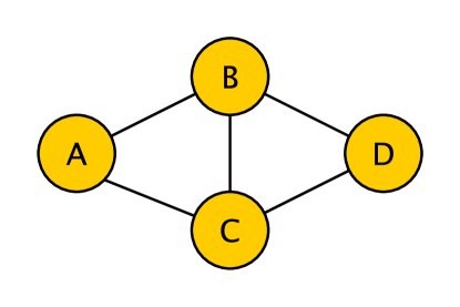
Figure 1: A sample with 4 vertices and 5 undirected edges. Vertices $A$ and $D$ are degree-2 vertices, and $B$ and $C$ are degree-3 vertices. All the edges in this graph have an SC value of $\frac{1}{2}$.

TABLE I: Notation used in the paper

Variable	Definition
$G=(V,E)$	Graph $G$ with vertices $V$ and edges $E$
$\Gamma(v)$	Neighbourhood of the vertex $v$ in $G$
$d(v)$	Degree of the vertex $v$, i.e., $|\Gamma(v)|$
$\textsc{SC}(e)$	The spanning centrality of $e$
$T(G)$	The spanning tree of the graph $G$
$\epsilon$	The absolute error threshold
$\delta$	The absolute error failure probability
$\omega$	The number of eigenvectors used
$\gamma$	The number of candidate nodes
$W_{[0..B)}$	A vector $W$ with $B$ elements
$p_{n}(v_{i},v_{j})$	a $n$-hop path between vertices $v_{i}$ and $v_{j}$

2.1 Spanning Centrality

Spanning centrality quantifies an edge’s (or implicitly a vertex’s) importance in maintaining the overall connectivity of a network. The metric is particularly valuable in analyzing electrical, social, sensor, and transportation networks, due to its ability to identify critical components that ensure network functionality [2, 4, 14, 18]. It provides valuable insights on the importance of each connection for network robustness, and hence, can contribute to strategic safeguarding and upkeeping of vital components, ensuring seamless network functionality.

For an undirected graph $G=(V,E)$, the spanning centrality of an edge $e\in E$, $\textsc{SC}(e)$ is defined as the fraction of spanning trees of $G$ that contain $e$ relative to the total number of spanning trees of the entire graph $G$. Hence, when $\textsc{SC}(e)=1$, the subgraph obtained by removing $e$ from the edge set, i.e., $G\setminus\{e\}$, is disconnected. Formally,

$$\textsc{SC}(e)=1-\frac{|T(G\setminus\{e\})|}{|T(G)|}$$

where $T(.)$ is a function that returns the number of spanning trees for a given graph. Unfortunately, $T$, therefore SC, is expensive to compute, especially for real-life networks.

In this work, we will be focusing on the problem of spanning centrality computation for all edges, i.e., All Edges Spanning Centrality (AESC). The current state-of-the-art [19] for AESC is based on Kirchoff’s matrix-tree theory and exhibits a time complexity of $\mathcal{O}(mn^{3/2})$. The time complexity renders exact computation infeasible for analyzing large graphs. Due to this, many approximation methods, based on random walks, have been proposed to overcome the computational burden [22, 17, 6, 13]. In the approximation setting, given the graph $G=(V,E)$, an $\epsilon$-approximation algorithm outputs $\hat{\textsc{SC}}(e)$ for each $e\in E$ such that

$$|\hat{\textsc{SC}}(e)-{\textsc{SC}}(e)|\leq\epsilon,~{}~{}\forall e\in E$$

where $\epsilon$ is an upper bound on the errors of reported SC values for all the edges.

2.2 Random Walks

A random walk in a graph $G=(V,E)$ can be defined as a sequence of vertices from $V$. In our setting, the walk $W=(v_{0},v_{1},\cdots,v_{t})$ starts from a given vertex $v_{0}\in V$, and each subsequent vertex $v_{i}$, $1\leq i\leq t$ is chosen uniformly at random from the neighbours of $v_{i-1}$, that is $v_{i}\in\Gamma(v_{i-1})$ for all $1\leq i\leq t$. The random choice function on a walk, $f(.)$, is often defined as one that selects a neighbouring vertex uniformly at random, as shown below:

$$v_{i}=f(v_{i-1})=\Gamma(v_{i-1})\left[{\cal R}~{}\bmod~{}d(v_{i-1})\right]$$ (1)

where ${\cal R}$ is a large random integer. That is the function first computes a random number between 0 and $d(v_{i-1})-1$ and returns the vertex with this index from $\Gamma(v_{i-1})$.

In this work, we would like to define random selection as a deterministic process, to utilize vectorization and increase the computational performance. We will denote random choice function $f(W_{id},v_{i-1},\ell)$ as a function of the ID of the random walk $W$, $W_{id}$, to which the new vertex is appended, vertex $v_{i-1}$ whose neighbourhood is used to select the new vertex (i.e., the next vertex of $W$), and length $\ell$ is the current length of $W$. Since random walks are time-reversible, this definition collapses the time dimension to the parameter $\ell$. By adding these additional parameters, we can extend the random walks so that all of them are independent of each other yet, as we will describe later, they become clusterable within Bouquets.

2.3 State-of-the-art in AESC approximation: TGT+

Truncated Graph Traversal (TGT), proposed by Zhang et al. [22], overcomes the limitations of other existing methods, e.g., [17, 6, 13], by strategically limiting the number of vertices/edges visited via judiciously truncated traversals. Zhang et al. also improved this algorithm in terms of both empirical efficiency and asymptotic performance while retaining result quality by proposing TGT+, combining TGT with random walks and employing additional heuristic optimizations. In this work, we have used TGT+ as a baseline to evaluate the performance of our random-walk processing scheme. We refer the reader to [22], but for completeness of this work, the TGT+ algorithm is described in Algorithm 1.

In a nutshell, TGT+ goes over each vertex $v_{i}\in V$ (the for loop at line 1) and processes in two main steps; After the initialization (lines 2–6), the first step (lines 8–15) calculates the number of hops $\tilde{\tau}$ after which the random walks will be taken into account. The reasoning is that the number of nodes near, i.e., within the $\tilde{\tau}$-neighbourhood, of $v_{i}$ is typically small, allowing for efficient coverage through a (breadth-first) graph traversal starting from $v_{i}$. In contrast, nodes that are farther away from $v_{i}$ can be numerous, potentially in the order of millions in large graphs. In such cases, random walks are more suitable, as they can prioritize exploring important nodes rather than attempting to cover all distant nodes. That is the algorithm considers the processing of $\tilde{\tau}$-neighbourhood of $v_{i}$ to be cheaper compared to a random-walk-based simulation.

The second step (the for loop within lines 16–22) iterates $n_{req}$ times, where $n_{req}$ is the required number of two-way random walks to reach sufficient accuracy. At each iteration, this step generates two random walks $W_{i}$ and $W_{j}$, starting from $v_{i}$, $v_{j}$, respectively. Then the vertices inside these length-$(\tau_{i,j}-\tilde{\tau})$ random walks $W_{i}$ and $W_{j}$ are used to improve edge centrality estimation where $\tau_{i,j}$ is the truncated length for each edge $\{v_{i},v_{j}\}\in E$ computed via using eigenvalues and eigenvectors of the matrix $\mathbf{D}^{-1/2}\mathbf{P}\mathbf{D}^{-1/2}$. Here, $\mathbf{D}$ is the diagonal, degree matrix and $\mathbf{P}=\mathbf{D}^{-1}\mathbf{A}$ is the random-walk transition probability matrix for a given $G$ with the adjacency matrix $\mathbf{A}$. More details and the exact definitions of the CalculateTau, NTrees, and CalculateChi functions can be found in the original work [22]. On the contrary, since the RandomWalk implementation will be the main focus of this work, it is given in Algorithm 2.

Algorithm 1 TGT+

Input: $G=(V,E)$: the graph
         $\epsilon$: The absolute error threshold
         $\delta$: The absolute error failure probability
         $\omega$: The number of eigenvectors used
         $\gamma$: The number of candidate nodes
Output: $\textsc{SC}(e)$: Estimated Spanning Centrality $\forall e\in E$

1:for $v_{i}\in V$ do

2:    $\forall v_{j}\in\Gamma(v_{i,j})~{}\tau_{i,j}\leftarrow$CalculateTau$(e_{i,j,\epsilon/2})$

3:    $p_{0}(v_{j},v_{i})\leftarrow 0~{}~{}\forall v_{j}\in{V}\setminus v_{i}$

4:    $p_{0}(v_{i},v_{i})\leftarrow 1~{}~{}\forall v_{i}\in{V}$

5:    $\hat{g}_{\tau}(v_{i},v_{j})\leftarrow 1/d(v_{i})~{}~{}~{}\forall v_{j}\in\Gamma(v_{j})$

6:    $n_{walks}\leftarrow\sum_{v_{j}\in\Gamma(v_{i})}$ NWalks$(e_{i,j},\tau_{i,j})$

7:    $l\leftarrow 0$

8:    while $\underset{v_{j}\in V\mbox{ \& }p_{l}(v_{j},v_{i})\neq 0}{\sum}d(v_{j})<n_{walks}$  do

9:         $p_{l}(v_{j},v_{i})\leftarrow 0~{}~{}\forall v_{j}\in{V}$

10:         for $v_{i}\in V\mbox{ s.t. }p_{l-1}>0$ do

11:             for $v_{x}\in\Gamma(v_{j})$ do

12:                 $p_{l}(v_{x},v_{i})\leftarrow p_{l}(v_{x},v_{i})+\frac{p_{l}(v_{j},v_{i})}{d(v_{i})}$                       

13:         $l\leftarrow l+1$

14:         $n_{walks}\leftarrow\sum_{v_{j}\in\Gamma(v_{i})}$ NWalks$(e_{i,j},\tau_{i,j}-l)$     

15:    $\tilde{\tau}\leftarrow l$

16:    for $v_{j}\in\Gamma(v_{i})\mbox{ s.t. }\tau_{i,j}-\tilde{\tau}>0$ do

17:         $\mathcal{X}\leftarrow$ CalculateChi$(G,v_{i},v_{j},{p}_{\tilde{\tau}}(v_{i}),\gamma)$

18:         $n_{req}\leftarrow$ NWalks$(e_{i,j},\tau_{i,j}-\tilde{\tau})$

19:         for $k=1\mbox{ to }n_{req}$ do

20:             $W_{i},W_{j}\leftarrow$ RandomWalk$(v_{i},v_{j},\tau_{i,j}-\tilde{\tau})$

21:             $X\leftarrow\sum_{v_{x}\in W_{i}}p_{\tilde{\tau}}(v_{x},v_{i})-\sum_{v_{y}\in W_{j}}p_{\tilde{\tau}}(v_{y},v_{i})$

22:             $\hat{g}_{\tau}(v_{i},v_{j})\leftarrow\frac{X}{n_{req}d(v_{i})}+\hat{g}_{\tau}(v_{i},v_{j})$              

23:for  $e_{i,j}\in E$ do

24:    $\hat{s}(e_{i,j})\leftarrow\hat{g}_{\tau}(v_{i},v_{j})+\hat{g}_{\tau}(v_{j},v_{i})$

25:return $\hat{s}(e_{i,j})\in E$

3 Approximate AESC with Bouquets

In this work, instead of handling the sampling and processing steps individually, we propose to fuse them within the course of a randomized algorithm. As explained later, this yields a memory-efficient lockstep processing scheme, which can be used to improve the regularization of the computation. The regularization can incur an improvement in both the spatial and temporal locality of the operations performed. Both of these allow more efficient use of contemporary computing resources especially when the computation and data layout incur highly irregular memory accesses such as sparse matrix, graph, and sparse tensor operations. As in many random-walk-based Monte Carlo simulations on graphs, in AESC, the random walk generation and processing are employed many times; each walk is processed individually, and each step in a walk iteratively samples only a single vertex to traverse. However, it is possible to rearrange the order of operations so that many random walk processes are run together.

The traditional random walk generation, given in Algorithm 2, can be simply implemented as follows: first, the algorithm sets the starting vertex of the walk $W$ and the current vertex $cur$ to $v$. Subsequently, it iterates the next $L-1$ steps where $L$ is the desired walk length. At each step $1\leq l\leq L-1$, it randomly selects one of $cur$’s neighbours and moves to that vertex using a random choice function at lines 4 & 5. The algorithm stores each visited vertex during the walk inside $W$ to track the path. In AESC, this process is repeated for the specified number, $n_{req}$, to generate multiple random walks starting from the same vertex via the loop at line of 19 Algorithm 1. When $n_{req}$ is large, which is the case for AESC especially if the desired approximation error is small, these walks share vertices which can be exploited via vectorization.

Algorithm 2 RandomWalk

Input:  $G=(V,E)$: the graph
          $v\in V$: starting vertex
         $L$: length of the random walk
Output: ${W}$: random walk

1:$W\leftarrow\mbox{ empty list of length }L$

2:$W[0]\leftarrow cur\leftarrow v$

3:for $l=1{\mbox{ to }}L-1$ do

4:     $k\leftarrow f(W,cur,l)$

5:     $cur\leftarrow\Gamma_{cur}[k]$ $\triangleright$ choose the $k$th vertex within $\Gamma_{cur}$

6:     $W[l]\leftarrow cur$

7:return $W$

3.1 Pseudo-Random Number Generation

The Linear Congruential Generator (LCG) was proposed by Thomson et al.[9] in 1951. It is one of the earliest and simplest pseudo-random number generators. The method produces a sequence of integers using a linear recurrence relation. The LCG algorithm is defined by the equation

$$X_{n+1}=(aX_{n}+c)\mod m,$$

where $X_{n}$ is the current pseudo-random number, $a$ is the multiplier, $c$ is the increment and $m$ is the modulus. LCG is very popular and available in many standard libraries including C language.

3.1.1 Mersenne Twister

The Mersenne Twister (MT), developed by Matsumoto and Nishimura in 1997 [12], is a widely used pseudo-random number generator known for its long period and high-quality randomness. The generator is based on a matrix linear recurrence over a finite binary field, providing a period of $2^{19937}-1$. It is available in the C++ standard library and its generator function compiles down to only a few instructions. The performance of Mersenne Twister was comparable to much simpler LCGs in our experiments.

3.1.2 Hash-based Random Number Generation

Hash-based random number generators are tools that generate pseudo-random numbers using hash functions. Unlike traditional pseudo-random number generators that use mathematical formulas to produce random-like sequences, hash-based RNGs rely on the properties of hash functions to generate unpredictable and uniformly distributed random numbers. In this work, we will adopt and extend the hash-based sampling method proposed by Gokturk and Kaya [5]. This method generates probability values over the edges while sampling them. Given a graph $G=(V,E)$, for an edge $\{u,v\}\in E$, it is defined by the following equation;

$$P(\{u,v\})_{r}=\frac{X_{r}\oplus h(u,v)}{h_{max}},$$ (2)

where $P(\{u,v\})_{r}$ is the pseudo-random number compared against the sampling probability of $\{u,v\}$ while generating the $r$th sample. In the equation, $h(u,v)$ is the hash value of the edge $\{u,v\}$, $X_{r}$ is a random seed for the $r$th sample which is unique for each sample, and $h_{max}$ is the maximum value the hash function can take. Since the random walk process can visit the same vertex multiple times, we cannot use the same method without modification. In this work, we will define our hash-based random number generators using a unique seed number for each path, the hash value of the vertex, and the hash value of the current path length to differentiate consequent visits to the same vertices.

3.2 Vectorized Random Walks via SIMD

Single Instruction Multiple Data (SIMD) is a parallelization technique that enables a single instruction to perform the same operation on multiple data items concurrently. SIMD units are available in almost all modern CPUs and GPUs to achieve computational efficiency for tasks allowing data-level parallelism. In these units, the data is often organized into vectors, and a single instruction is applied to all elements in the vector. Modern processors often feature SIMD instruction sets such as Intel’s AVX2 (Advanced Vector Extensions 2) or ARM’s NEON. These instructions typically provide very high throughput, though they may have slightly higher latency; i.e., it is common for an AVX2 instruction to have 0.5 cycles per instruction and 4-cycle latency. Although vectorization can significantly improve performance, with the traditional random-walk generation process, exploiting the CPU’s vector capabilities is impossible since each step lengthens a single walk by one.

In GPUs, SIMD-capable units are known as Streaming Multiprocessors (SMs) or Compute Units (CUs). Each SM/CU contains multiple SIMD lanes called warps/wavefronts that process data in a SIMD fashion. Most common operations are done on multiple data elements of a lane in a single cycle. Warps consist of 32 threads, and wavefronts are usually formed by 32 or 64 threads. In this work, although we have implemented our methods only using AVX2 intrinsics on the CPU, we believe that the techniques can also be applied while generating random walks on GPUs.

The basic random walk generation process given in Algorithm 2, by its design, is not SIMD friendly and furthermore, incurs an unpredictable memory access pattern. In simple terms, the algorithm performs iterative random number generation and random neighbour selection. The state-of-the-art RNGs only require a few simple instructions like integer addition and exclusive-or. In addition, the (short) latency of these instructions can be hidden which makes them negligible compared to overall runtime. This leaves edge traversal, i.e., random memory access, as the major bottleneck for the performance.

Since each walk is independently sampled, the same memory region can be accessed many times in different walks due to their shared vertices and neighbourhoods. In addition, the expensive modulus operation executed while selecting the new vertex has a long latency that cannot be hidden since its result is immediately required. Both problems can be remedied by properly scheduled vectorized random walks, i.e., bouquets, especially when the number of random walks to be processed is large enough.

Algorithm 3 RandomBouquet

Input: $v\in V$: starting vertex
         $L$: length of the random walk
         $B$: SIMD vector size/#random walks
Output: $\{W_{0},\dots,W_{B-1}\}$: $B$ random walks, i.e., a bouquet

1:$W_{b}\leftarrow$ empty list of length $L$, for $0\leq b<B$

2:$cur_{b}\leftarrow v$, for $0\leq b<B$

3:for $l=1{\mbox{ to }}L-1$ do

4:     $k_{b}\leftarrow f(W_{b},cur_{b},l)$, for $0\leq b<B$

5:     $cur_{b}\leftarrow\Gamma_{k_{b}}(cur_{b})$, for $0\leq b<B$

6:     $W_{b}[l]\leftarrow cur_{b}$, for $0\leq b<B$

7:return $\{W_{b}:~{}0\leq b<B$}

The RandomBouquet algorithm given in Algorithm 3 samples multiple random walks concurrently, instead of generating them individually. The algorithm coarsely aligns operations to allow the use of SIMD/SIMT. First, all $cur_{b}$ registers are initialized with the starting vertex $v$ (line 2). Then, pseudo-random numbers, $k_{b}$, are generated for all random walk instances $W_{b}$ where $0\leq b<B$. This step, at line 4 in algorithm 3, can be fully vectorized as discussed later. Next, the $k_{b}$th neighbour of $cur_{b}$ is selected for all $0\leq b<B$ and each $cur_{b}$ is set to the corresponding, randomly chosen vertex. In practice, the selection operation can be divergent and require memory accesses with bad spatial locality (or uncoalesced memory accesses on a GPU) which will probably overhaul the benefit of vectorization. However, these accesses can be done efficiently by selecting spatially close vertices. Finally, the selected vertices are used to lengthen their corresponding random walks, and the algorithm continues with the next iteration. An improved bouquet arrangement and vertex selection scheme are proposed in the next subsection.

3.3 SABA: Sampling-Aware Bouquet Arrangement

Sampling-aware bouquet arrangement (SABA) arranges the random walks with respect to their potential memory accesses by manipulating and exploiting the underlying random number generation scheme. In a naive random-walk implementation, let $cur\in V$ be the current vertex for a random walk $W$. The straightforward neighbour-vertex sampling, shown in (3), generates a pseudo-random number and constrains the result within the cardinality of the current vertices neighbourhood using the modulus operator which induces a significant latency.

$$f(W,cur,l)=rand()~{}\bmod~{}d(cur)$$ (3)

This approach allows us to process a single walk at a time and generates the walk by sampling each neighbouring vertex on the fly. Figure 2(a) shows the case where 8 random walks, $W_{0}$ to $W_{7}$, are generated one after another. Hence, Algorithm 2, RandomWalk, is called 8 times to generate these walks. Algorithm 3 can also be used for random walk generation. Figure 2(b) shows the generation of the same set of walks in batches of size four, with two executions of RandomBouquet and $B=4$. For the first batch/execution, the starting vertices of $W_{0}$ to $W_{3}$ are set and their second vertices are randomly chosen at once. Lastly, their final vertices are chosen. Then the execution continues with the next batch, i.e., the walks $W_{4}$ to $W_{7}$.

Processing multiple random walks allows us to perform vectorized operations for computations including vertex selection and random number generation. However, when the corresponding memory accesses require different cache lines as in Fig. 2(b), the performance of the memory subsystem becomes the bottleneck. Our approach seeks to remedy this by trying to sample similar paths together.

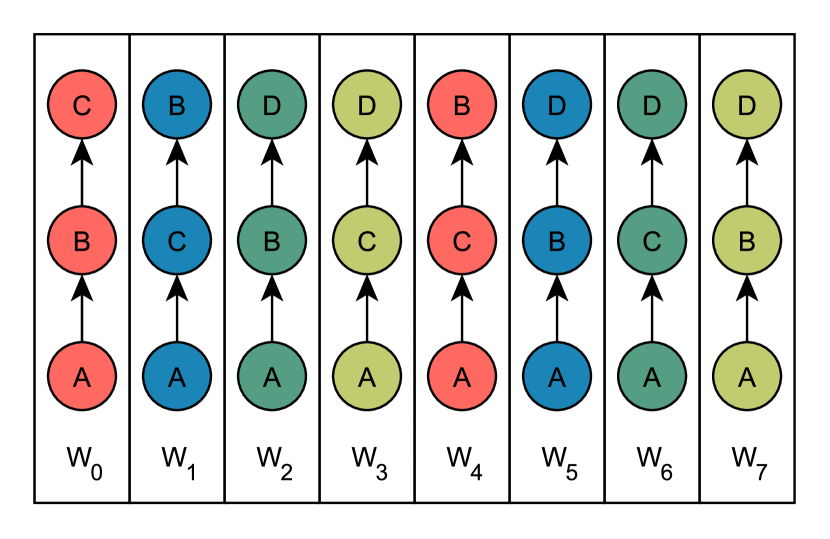
(a) Sequential, non-vectorized processing of the walks in the order of their IDs.

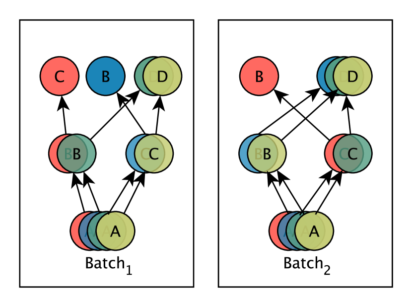
(b) Vectorized processing of the walks with a SIMD unit. Each SIMD unit is assumed to process four random walks.

Figure 2: A set of random walks generated from the sample graph in Fig. 1 with no judicious arrangement (top) and their vectorized execution (bottom).

The hash-based random number generation is regulated by combining two parts;

1. a unique, independently chosen random seed $\mathcal{X}$ generated for each random process, i.e., a walk, and

2. a random number obtained from the current state of the corresponding random process.

These two are then XOR’ed to generate a pseudo-random number. For random walks, this translates to

$$f(W,cur,l)=\mathcal{X_{W}}\oplus h(cur,l)\bmod~{}d(cur)$$ (4)

where, $\mathcal{X}_{W}$, the random seed for walk $W$ is the same for all randomly selected vertices to generate $W$. The latter part helps to randomly choose the next vertex where $cur$ is the current vertex. Note that $l$ is required inside the hash function since it completes the definition of the current state and we do not want the walk to go into an infinite loop and always continue with the same neighbour from $cur$. Since $\mathcal{X_{W}}$s are generated before the walks are generated, they can be exploited to improve the performance.

Sorting the walks with respect to their $\mathcal{X}_{W}$s and using (4) can improve cache locality at the first step, i.e., the first iteration of the loop at line 3 of Alg. 3, since $h(cur,1)$ is the same and the selected vertices will be close to each other, i.e., probably in the same cacheline, for walks with close $\mathcal{X}_{W}$ values. However, the later steps/iterations will still suffer from memory accesses since the selected vertices will come from different neighbourhoods. Hence, (4), even with sorting, does not help much to improve spatial locality.

Sampling-aware bouquet arrangement (SABA) uses the hash-based RNG scheme given in (5) and arranges the walks within bouquets by ordering their random seeds $\mathcal{X}_{W}$;

$$f(W,cur,l)=\left\lfloor\frac{{\mathcal{X}}_{W}\oplus h(cur,l)}{h_{max}}\times d(cur)\right\rfloor$$ (5)

where $h_{max}$ is the maximum value the hash function can take. One small detail is that the pseudo-random number is first normalized and scaled to range $0\leq f(W,cur,l)<d(cur)$ via a division and multiplication instead of the expensive modulus operation.

The main benefit of SABA is that sorting the walks w.r.t. their random seeds now helps similar walks to be consecutive in a group, which we call a bouquet. This is because smaller seeds are likely to have flips in their lower bits and larger seeds are likely to have flips in the higher bits. Furthermore, since there are no wraparounds as in the modulus used in (4), the random numbers generated for the walks in a bouquet are likely to be the same, especially in the earlier steps/iterations. That is as we will show in the experiments, SABA improves the cache hit rate of RandomBouquet given in Alg. 3 by forcing the random walks generated at once to be similar.

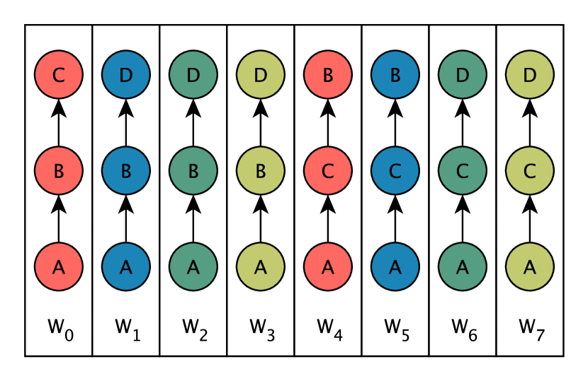
(a) Sequential, non-vectorized processing of the walks in the order of their seed, $\mathcal{X}$, values.

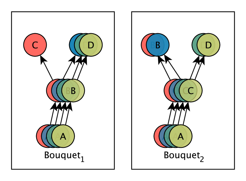
(b) Vectorized processing of the walks with a SIMD unit. Each SIMD unit processes four random walks.

Figure 3: A set of random walks generated from the sample graph in Figure 1 with SABA (top) and their vectorized execution (bottom).

In Fig. 2, the first batch starts with $A$ and in the first step, it follows $B$ and $C$ from $A$’s neighbourhood. Depending on the distance of $B$ and $C$ in memory, at most two cache lines may be read. In the second step, $C$ and $D$ (from $\Gamma(B)$) and $B$ and $D$ (from $\Gamma(C)$) are chosen. A simple observation is that the number of distinct vertices at each step is an important metric to minimize. Assuming a relatively small cache size, and considering that there exist millions of vertices in a graph, arranging the walks to make similar ones processed together can optimize the performance. Indeed, when paths are organized as in Figure 3, only one vertex, $B$ and $C$, are accessed for the first and second batch, respectively, in the first step. Similarly, for the second step of both batches, the number of vertices accessed is two instead of three with SABA.

4 Implementation Details for AESC

The TGT+ algorithm is sequential but an almost pleasingly parallel algorithm with a small exception. In Alg. 1, the work can be divided into sub-tasks on the very first line. However, this would increase the memory requirements linearly w.r.t. the number of cores/threads used. The only race condition is on line 22, where $\hat{g}_{\tau}$ is updated. A simple solution is accumulating $\hat{g}$ for each thread and reducing values to single $\hat{g}$ after the loop between lines 1–22. In our experiments, this approach has no significant measurable overhead compared to total run time.

The original TGT+ implementation relies on sparse data structures like unordered_map to store edge-specific information. Swapping compilers and tweaking compilation flags can significantly increase the performance of the original implementation. Instead of relying on compiler optimizations, in our implementation, we have refrained from using these data structures. Wherever intermediate data structures are used, e.g., $\hat{g}_{\tau}$, we have skipped these steps and accumulated values directly to the final results as stated above.

We have used explicit AVX2 intrinsics to exploit instruction-level parallelism for hashing, XOR, and multiplication operations for generating random numbers. All division operations are converted to multiplications by precomputing the inverse of the divisors. Besides explicit vectorization using AVX2 intrinsics, we have vectorized the modulus operation for the baselines using _mm256_rem_epu32 intrinsics available in Intel SVML extension.

Even though TGT+ is fast, it has been significantly outperformed by our implementation. In single-thread experiments, our approach has $24\times$ speed-up on average with $8$-wide vector instructions. Ignoring SABA’s impact on reducing cache misses, the speedup must be lower than $8\times$ since vector instructions have more latency. We performed synthetic experiments focusing only on random walks to isolate the speedups due to SABA from those of other performance tweaks on TGT+. In these synthetic experiments, each thread runs a constant number of, fixed-length random walks from one vertex and then moves to the next. No scheduling optimization is done to skew the results, only single OpenMP parallel for the directive is used on the most outer loop for parallelization. After random paths are sampled, we count the vertices in those paths to introduce a small path processing step, that is excluded from our timings, to prevent the compiler from removing the computations during its optimization stages.

5 Experimental Results

The experiments are conducted on a server with a 16-core Intel(R) Xeon(R) E5-2620 v4 CPU, running at fixed 2.10GHz , and 189GB memory. The operating system on the server is Ubuntu Linux with 5.4.0-167 kernel. The CPU algorithms are implemented using C++20, and compiled with Intel C++ Compiler 2023.2.1 with "-Ofast" and "-march=native" optimization flags. Multithreading is achieved with OpenMP pragmas. AVX2 instructions are utilized by handcrafted code with vector intrinsics.

TABLE II: Properties of networks used in the experiments

	No. of	No. of	Avg.	Dia-
Dataset	vertices	edges	degree	meter
Facebook	4,039	88,234	21.85	8
Twitch	9,498	153,138	16.12	21
HepTh	12,008	118,521	9.87	13
HepPh	34,546	421,578	12.20	12
Gnutella	62,586	147,892	2.36	11
Epinions	75,879	508,837	6.70	14
Slashdot	82,168	948,464	11.54	11
Orkut	3,072,441	117,185,083	38.14	9

The experiments are performed on eight graphs. The properties of these graphs are given in Table II: DBLP is DBLP collaboration network, Facebook is friendship ego-network of a survey app, HepPh is a physics citation network, and Twitch is a steamer friendship network. All graphs are retrieved from Stanford Large Network Dataset Collection [10].

We design two benchmark settings for a comprehensive experimental evaluation. For each network, we perform experiments with a;

1. Synthetic benchmark: These experiments are done using the product of the following parameter set;

   • Random walk length: 5, 10 and 15.

   • Number of random walks per vertex: 2048 and 16384.

2. AESC benchmark compared to TGT+ [22]: These experiments are done with the default error parameter $\epsilon=0.05$ as the authors also did.

With these benchmarks, we aim to measure performance gains obtained via SABA on both real-world AESC computations where many, usually short, random walks per vertex are generated and processed as in TGT+, and a hypothetical use case where a large number of walks as in our synthetic benchmarks.In all these benchmarks, we measure the total time spent on the actual computation, excluding parsing the datasets and pre-processing.

5.1 Randomness Tests

We performed Diehard Randomness tests [11] to validate our pseudo-random number generation scheme. Diehard Randomness is a suite of statistical tests designed for assessing the quality and randomness of pseudorandom number generators (PRNGs). The suite consists of many tests that evaluate the sequence of numbers generated by PRNGs against the expected statistical properties of well-established pseudorandom sequences. We have used Dieharder Suite[1] and tests are done against Mersenne Twister implementation in C++ STL.

We note that when consecutive random numbers used in bouquets are inspected, they are correlated. Most of the performance gains come from similar walks that are being clustered as they are generated. However, due to the independently generated random seeds, there are no data dependencies among bouquets, i.e., their progress is independent. For a fair assessment, we recorded random numbers generated for every individual path separately and merged all of the numbers afterwards. It can be viewed as the data is collected with a stride of the same length as the number of random walks performed per vertex.

TABLE III: Diehard randomness test results for the proposed PRNG method used in SABA. PRNG values are generated for $16384$ random walks from all vertices in the Facebook dataset. $t$samples is the number of tests where each is repeated $p$samples times. We refer the reader to [11] for the explanation of the tests.

Test	$t$samples	$p$samples	$p$-value	Assessment
birthdays	100	100	0.69297256	$\checkmark$
operm5	1,000,000	100	0.15598509	$\checkmark$
rank_32x32	40,000	100	0.81167703	$\checkmark$
rank_6x8	100,000	100	0.02556901	$\checkmark$
bitstream	2,097,152	100	0.26712938	$\checkmark$
opso	2,097,152	100	0.27306982	$\checkmark$
oqso	2,097,152	100	0.61151153	$\checkmark$
dna	2,097,152	100	0.58618161	$\checkmark$
count_1s_str	256,000	100	0.75938339	$\checkmark$
count_1s_byt	256,000	100	0.85422106	$\checkmark$
parking_lot	12,000	100	0.37131003	$\checkmark$
2dsphere	8,000	100	0.44102237	$\checkmark$
3dsphere	4,000	100	0.81857171	$\checkmark$
squeeze	100,000	100	0.64661078	$\checkmark$
sums	100	100	0.42462152	$\checkmark$
runs	100,000	100	0.93317038	$\checkmark$
craps	200,000	100	0.52659196	$\checkmark$

Table III shows the exact output of Diehard experiments performed, i.e., $p$-values of each test and validity assessment. The pseudo-random number generation we have used in SABA is assessed as acceptable in all the tests. Even in some of the tests the proposed has a low $p$-value, the value has never fallen below the $0.025$ threshold and is acceptable for non-cryptographic use, such as the Monte-Carlo simulations in this work. Note that we also tested the accuracy of the spanning centralities of the edges obtained, and compared them with those obtained from the original TGT+ to verify the soundness of the PNRG and our TGT+ implementation.

5.2 Effects of Bouquets on Cache

We have described bouquets as a technique to obtain pseudo-randomness while focusing on the performance; from another perspective, bouquets perform best-effort, zero-shot spatial ordering of walks. Scheduling random walks in an order that keeps the similar vertices together in a bouquet can reduce cache misses drastically as shown in Table IV. As the third, AVX2, column of the table shows, vectorization has a significant overhead of calculating multiple random values, which increases memory pressure; on average $29\%$ more cache misses are observed when the naive method is directly vectorized, 8 random values are generated consecutively and only the modulo-based randomized selection,

$$rnd(.)~{}\bmod~{}d(v),$$

operation is done using AVX2 instructions.

The next method uses a hash-based PRNG (as in (2)) in addition to vectorization, which allowed us to free more registers and reduce memory pressure by removing the need to access seed values on main memory. This approach, labelled as HASH in the fourth column of the table, shows $20\%$ reduction in cache-misses than the naive approach. However using this approach, all vertices in the vector are expected to be different, and multiple random accesses are required for each step. As the last column shows, SABA significantly improves HASH by clustering the same/close vertices in the same vector and making consecutive memory accesses available in the cache. This approach reduces cache misses by $97.3\%$ on average.

TABLE IV: Number of cache misses for the naive approach, given in the second column, compared to the SIMD-based methods while processing 16,384 random walks for each vertex. The other methods are given as their percentage of the naive approach.

Dataset	Naive	AVX2	HASH	SABA
Facebook	845,487,783	134.95%	128.89%	1.49%
Twitch	41,381,402,038	114.69%	20.55%	6.22%
HepTh	2,286,294,504	133.06%	101.75%	4.84%
HepPh	2,891,186,237	127.86%	89.99%	3.15%
Gnutella	4,244,404,537	127.55%	46.79%	0.64%
Epinions	6,961,063,497	132.59%	76.46%	2.54%
Slashdot	7,210,297,453	119.48%	48.83%	0.50%
Orkut	1,077,204,257,701	142.17%	123.23%	2.18%
Min.		114.69%	20.55%	0.50%
Mean		129.04%	79.56%	2.70%
Max.		142.17%	128.89%	6.22%

In a vectorized code, every distinct vertex in a vector causes random walks to branch out, visit more vertices, and create branches. These branches cause more random memory access that is unlikely to be in the cache and slows the execution. Table V shows the branching statistics of different scheduling/PRNG methods; the table shows the number of distinct elements for the $1\%$th, $10\%$th, and $25\%$th 8-wide vector with the least branches on the Facebook dataset. In addition, the last column shows the average. The experiment shows that without SABA, almost all the elements in a vector are expected to be different (7.91/7.96 distinct elements per 8 elements). However, with SABA, only $5.33$ elements are expected to be distinct. Furthermore, the distinct vertices inside the vectors will be the central vertices likely to be sampled more which will probably incur fewer cache misses. In addition to the average value, AVX2 and HASH techniques have almost all distinct sets whereas SABA’s bouquets will have only a single branch in the $1^{st}$ percentile and two branches in the $10^{th}$ percentile.

TABLE V: Branching statistics for random walks, using 8-wide vectors and $16384$ random walks per vertices on Facebook dataset. The values are given for $1^{st}$, $10^{th}$, $25^{th}$ percentiles and mean.

Method	$1^{st}$	$10^{th}$	$25^{th}$	Mean
AVX2	7	8	8	7.91
HASH	7	8	8	7.96
SABA	1	2	4	5.33

5.3 Performance on AESC Benchmark

We first checked that on the AESC benchmark, our implementation matched the quality of TGT+. Compared to exact computation, TGT+ has an error rate of at most $15\times 10^{-4}$ with $\epsilon=0.005$, whereas the error rate of our method is $8\times 10^{-4}$. Since the same algorithm is used in both cases, we can argue that the hash-based sampling using Murmur2 performed as well as the Linear Congruential Generator used in the original TGT+.

The proposed AESC implementation performed better than the original TGT+ on every experiment setting as shown in Table VI. The mean speed-up is approximately $24.1\times$ on single-thread execution of TGT+. We have elected not to include multi-threaded experiment results for TGT+ due to its single-thread design. Adding OpenMP directives to parallelize TGT+ without any modification to the rest of the algorithm unfairly causes false sharing and excessive cache-trashing, drastically affecting the multicore performance. We only report the speedup of our multi-threaded implementation with respect to TGT+ for completeness. Table VI also shows the scalability results of the proposed implementation. Overall, compared to the single-thread performance, our AESC implementation with SABA becomes $8.2\times$ faster on average with 16 threads. The single-thread speedups for $\epsilon=0.005$ are visualized in Figure 4.

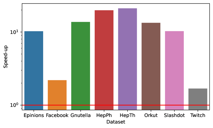
Figure 4: Speed-up achieved against TGT+ implementation via a single thread and $\epsilon=0.005$.

TABLE VI: Execution times (in secs) of All Edge Spanning Centrality methods. (*) For Orkut, we processed 5% of the edges (the same edges for all experiments) due to its long runtime; the time is multiplied by 20 to give an estimate.

	Method	TGT+	SABA
Dataset	$\epsilon$/#Threads	1	1	2	4	8	16
Facebook	0.005	2.47	1.13	0.57	0.31	0.20	0.13
	0.01	1.78	0.56	0.29	0.17	0.11	0.07
	0.05	1.32	0.12	0.08	0.05	0.02	0.02
Twitch	0.005	1448.08	858.68	442.48	225.82	121.47	69.91
	0.01	701.22	381.53	187.69	96.33	52.07	30.34
	0.05	246.03	43.38	22.17	11.74	6.55	4.18
HepTh	0.005	8.01	0.38	0.21	0.14	0.10	0.06
	0.01	8.02	0.38	0.20	0.14	0.10	0.06
	0.05	7.71	0.39	0.23	0.15	0.10	0.06
HepPh	0.005	9.81	0.49	0.28	0.16	0.11	0.07
	0.01	9.24	0.48	0.26	0.18	0.12	0.07
	0.05	9.24	0.49	0.26	0.17	0.12	0.07
Gnutella	0.005	8.57	0.62	0.32	0.21	0.14	0.10
	0.01	8.16	0.62	0.34	0.19	0.14	0.11
	0.05	8.21	0.64	0.32	0.18	0.12	0.10
Epinions	0.005	14.13	1.38	0.73	0.41	0.30	0.24
	0.01	14.50	1.36	0.71	0.41	0.29	0.24
	0.05	13.99	1.36	0.72	0.41	0.31	0.23
Slashdot	0.005	16284.05	1584.08	796.14	402.50	220.57	127.25
	0.01	13260.48	1031.39	515.72	261.35	143.30	83.27
	0.05	7174.20	220.21	110.02	55.75	30.66	17.85
Orkut*	0.005	1306407.50	97803.97	55767.43	30785.56	17920.59	11163.80
	0.01	1032411.82	33182.23	18495.36	10533.28	6225.73	3914.93
	0.05	582976.16	2227.20	1223.31	685.08	404.73	248.56
Mean speedup w.r.t. original TGT			$24.08\times$	$44.46\times$	$77.54\times$	$126.80\times$	$203.01\times$
Mean speedup w.r.t. single thread			$1.00\times$	$1.88\times$	$3.28\times$	$5.31\times$	$8.20\times$

5.4 Performance on Synthetic Benchmarks

The $24.08\times$ speedup over TGT+ reported in Table VI includes the impact of memory-related performance tweaks we used in our implementation. Instead of dissecting TGT+, which has state-of-the-art performance [22], we show the performance improvement of the bouquet-based random walk processing strategy via a set of synthetic experiments. For each graph, we processed a predefined number of random walks starting from each vertex until a predefined depth is reached. These random walks are processed as they are traversed and only vertex visit count is stored similar to what TGT+ does during AESC computations.

The results of the synthetic benchmark are given in Table VII. The results show that vectorization consistently improves the random-walk processing performance. With a step-by-step analysis, we see that AVX2, which also uses vectorization on the modulus operator used to select vertices, provides $33\%$ performance improvement. A significant portion of this speedup is due to reducing the modulus operation to a quarter of its time on average. When hash-based PRNG is used with vectorization, the improvement increases to 42%. Nevertheless, the main performance improvement comes with bouquets; SABA achieves $\approx 7.8\times$ on average and up to $\approx 14\times$ speedup compared to the naive random-walk processing strategy. This difference in speedups is visualized in Figure 5 for the case with 16384 walks of length 15.

TABLE VII: Execution times (in secs) of the random walk generation/processing approaches mentioned in this work using 16 threads.

Dataset	#Walks	Length	Naive	AVX2	HASH	SABA
Facebook	2048	5	0.16	0.18	0.19	0.03
		10	0.35	0.36	0.37	0.06
		15	0.54	0.54	0.53	0.10
	16384	5	1.30	1.43	1.44	0.20
		10	2.29	2.90	2.81	0.35
		15	3.63	4.36	4.31	1.03
Twitch	2048	5	10.29	6.52	3.73	1.32
		10	25.22	13.02	7.12	2.53
		15	40.34	18.83	9.55	3.67
	16384	5	78.06	49.68	28.70	9.71
		10	198.34	98.80	59.43	17.72
		15	320.38	145.75	99.65	22.93
HepTh	2048	5	0.65	0.60	0.51	0.14
		10	1.50	1.19	0.93	0.23
		15	2.44	1.79	1.33	0.34
	16384	5	5.13	4.76	4.10	1.02
		10	11.97	9.52	9.48	1.57
		15	19.37	14.28	10.61	3.53
HepPh	2048	5	0.82	0.71	0.58	0.18
		10	1.93	1.42	1.07	0.30
		15	3.08	2.13	1.51	0.42
	16384	5	6.44	5.66	4.61	1.22
		10	15.37	11.31	8.47	1.97
		15	24.55	16.96	11.90	3.00
Gnutella	2048	5	1.25	1.17	0.77	0.20
		10	3.24	2.33	1.32	0.38
		15	5.30	3.49	1.73	0.56
	16384	5	9.84	9.30	6.19	1.49
		10	25.77	18.56	10.74	2.94
		15	42.13	27.66	14.04	4.39
Epinions	2048	5	1.93	1.71	1.41	0.29
		10	4.50	3.39	2.45	0.52
		15	7.06	5.05	3.51	0.79
	16384	5	15.48	13.52	10.99	1.96
		10	35.77	26.97	54.04	4.15
		15	56.26	40.65	26.27	6.18
Slashdot	2048	5	2.04	1.70	1.17	0.26
		10	4.79	3.38	2.01	0.48
		15	7.61	5.07	2.78	0.72
	16384	5	16.14	13.52	9.24	1.87
		10	38.20	26.99	18.25	3.70
		15	60.69	40.47	27.49	5.57
Orkut	2048	5	251.99	244.67	198.15	57.13
		10	679.28	484.48	384.18	106.00
		15	1118.66	727.29	557.54	150.29
	16384	5	1829.83	1944.52	1555.43	350.68
		10	5341.31	3823.49	2969.43	559.12
		15	8701.35	5789.93	4420.55	755.48
Mean speedup				$1.33\times$	$1.90\times$	$7.80\times$
Max speedup				$2.20\times$	$4.22\times$	$13.97\times$

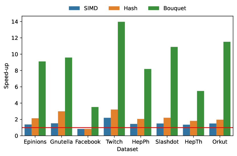
Figure 5: Speed-up achieved against naive implementation using 16-threads. Walk length=15, number of walks = 16384.

5.5 Limitations on Performance

The proposed technique bets on the walks containing repeated elements to be efficient. When duplicates are present in Bouquets, the edges can be retrieved from the cache. Otherwise, even with bouquets, the same number of retrievals are done with additional register and memory pressure.

For a bouquet with $\alpha$ random walks, let $\beta$ be the number of elements the samples are coming from and $\eta$ be the number of distinct items in a single level of a Bouquet. The ratio of the number of distinct items to the number of selected items can be written as

$$E(\eta) =\frac{\beta}{\alpha}\times\left(1-\left(1-\frac{1}{\beta}\right)^{\alpha}\right)$$ (6)

$$=\frac{\beta}{\alpha}\times\left(1-e^{\frac{-\alpha}{\beta}}\right)$$ (7)

Intuitively, independently sampling a small number of vertices from a large number of vertices, e.g. $\beta\gg\alpha$, makes duplicate items not frequent. In a graph, a large $\beta$ implies a hub-vertex. This makes SABA expected to perform better on networks without large hubs like road networks. In contrast, networks with long-tailed degree distribution such as social networks, can reduce the number of repeated samples. On such networks, although SABA performs less than optimal, it still performs much better than the Naive approach in our experiments. This being said, even in the existence of hub vertices, an extremely large number of random walks make vertices repeat enough number of times. Note that AVX2 registers can store 8 values and more than tens of repetitions is enough. Similarly, when walks are short, Bouquets are likely to have a low branching factor and the overall performance will be superior. However, when walks are longer, the performance at later levels will be limited.

6 Related Work

In the literature, there exist two ways to improve random walk performance on graphs; first, approximation methods can utilize underlying graph structures to generate diffusion matrices that estimate the probability of random walk visits. ARK, proposed by Kang et al. [8], utilizes low-rank structures of graphs and estimates random walk diffusion processes using a few ranks of eigenvectors. In addition, Sarma et al. proposed several algorithms [3] that employ dynamic programming to improve the asymptotic performance of random-walk problems, including destination-only $k$-random walks, source-destination pair $k$-random walks, and only path position of vertices from $k$-random walks. In AESC, low-rank eigenvector methods can introduce errors, and they do not perform well for a relatively small number of walks or sources. Existing dynamic programming methods focus on single-source walks and might not be applicable when every step of the walk is required to be processed, i.e., when the vertices are required, in order as in the case of AESC.

The second category of performance improvements is utilizing compute resources efficiently, SkyWalker+, proposed by Wang et al. [21], uses compressed aliasing and speculative execution to speed up random walk workloads. There also exists a GPU-based method, C-Saw, proposed by Pandey et al. [15], that exploits the sampling stage to improve performance and uses inverse transform sampling. A similar approach is applied by NextDoor, proposed by Jangda et al. [7], via rejection sampling. These methods, even though they may be relevant, do not focus on CPU vectorization and spatial locality.

7 Conclusion

In this work, we presented a sampling-aware random walk method that clusters paths as bouquets. We tested the proposed approach on a real-world use case, All Edges Spanning Centrality. Using the proposed techniques, we provide a fast AESC implementation that utilizes multi-threading and AVX2 instructions. We compared the performance with state-of-the-art AESC implementations such as TGT+ on real-world datasets and illustrate that our implementation can be an order of magnitude faster.

Gökhan Göktürk is an independent researcher. He has received his BS, MS, PhD degrees from Sabancı University. He is interested in High Performance Computing, Parallel Programming, and Graph Processing.

Kamer Kaya is an Associate Professor at the Faculty of Engineering and Natural Sciences at Sabancı University. He got his PhD from Dept. Computer Science and Engineering from Bilkent University. He worked at CERFACS, France, as a post-graduate researcher in the Parallel Algorithms Project. He then joined the Ohio State University in September 2011 as a postdoctoral researcher, and in December 2013, he became a Research Assistant Professor in the Dept. of Biomedical Informatics. His current research interests include Parallel Programming, High Performance Computing, and Cryptography.

References

- [1] R. G. Brown, D. Eddelbuettel, and D. Bauer, “Dieharder,” Duke University Physics Department Durham, NC, pp. 27 708–0305, 2018.
- [2] A. Cuzzocrea, A. Papadimitriou, D. Katsaros, and Y. Manolopoulos, “Edge betweenness centrality: A novel algorithm for qos-based topology control over wireless sensor networks,” Journal of Network and Computer Applications, vol. 35, no. 4, pp. 1210–1217, 2012.
- [3] A. Das Sarma, D. Nanongkai, G. Pandurangan, and P. Tetali, “Distributed random walks,” J. ACM, vol. 60, no. 1, feb 2013. [Online]. Available: https://doi.org/10.1145/2432622.2432624
- [4] M. Girvan and M. E. Newman, “Community structure in social and biological networks,” Proceedings of the national academy of sciences, vol. 99, no. 12, pp. 7821–7826, 2002.
- [5] G. Göktürk and K. Kaya, “Boosting parallel influence-maximization kernels for undirected networks with fusing and vectorization,” IEEE Transactions on Parallel and Distributed Systems, vol. 32, no. 5, pp. 1001–1013, 2020.
- [6] T. Hayashi, T. Akiba, and Y. Yoshida, “Efficient algorithms for spanning tree centrality.” in IJCAI, vol. 16, 2016, pp. 3733–3739.
- [7] A. Jangda, S. Polisetty, A. Guha, and M. Serafini, “Nextdoor: Gpu-based graph sampling for graph machine learning,” ArXiv, vol. abs/2009.06693, 2020. [Online]. Available: https://api.semanticscholar.org/CorpusID:221703383
- [8] U. Kang, H. Tong, and J. Sun, “Fast random walk graph kernel,” in Proceedings of the 2012 SIAM international conference on data mining. SIAM, 2012, pp. 828–838.
- [9] D. H. Lehmer, “Mathematical models in large-scale computing units,” Ann. Comput. Lab.(Harvard University), vol. 26, pp. 141–146, 1951.
- [10] J. Leskovec and A. Krevl, “SNAP Datasets: Stanford large network dataset collection,” http://snap.stanford.edu/data, Jun. 2014.
- [11] G. Marsaglia. (1995) The marsaglia random number cdrom including the diehard battery of tests of randomness. [Online]. Available: http://stat.fsu.edu/pub/diehard/
- [12] M. Matsumoto and T. Nishimura, “Mersenne twister: a 623-dimensionally equidistributed uniform pseudo-random number generator,” ACM Transactions on Modeling and Computer Simulation (TOMACS), vol. 8, no. 1, pp. 3–30, 1998.
- [13] C. Mavroforakis, R. Garcia-Lebron, I. Koutis, and E. Terzi, “Spanning edge centrality: Large-scale computation and applications,” in Proceedings of the 24th international conference on world wide web, 2015, pp. 732–742.
- [14] M. E. Newman and M. Girvan, “Finding and evaluating community structure in networks,” Physical review E, vol. 69, no. 2, p. 026113, 2004.
- [15] S. Pandey, L. Li, A. Hoisie, X. Li, and H. Liu, “C-saw: A framework for graph sampling and random walk on gpus,” in 2020 SC20: International Conference for High Performance Computing, Networking, Storage and Analysis (SC). Los Alamitos, CA, USA: IEEE Computer Society, nov 2020, pp. 780–794. [Online]. Available: https://doi.ieeecomputersociety.org/10.1109/SC41405.2020.00060
- [16] K. Pearson, “The problem of the random walk,” Nature, vol. 72, no. 1865, pp. 294–294, 1905.
- [17] P. Peng, D. Lopatta, Y. Yoshida, and G. Goranci, “Local algorithms for estimating effective resistance,” in Proceedings of the 27th ACM SIGKDD Conference on Knowledge Discovery & Data Mining, 2021, pp. 1329–1338.
- [18] J. Scheurer and S. Porta, “Centrality and connectivity in public transport networks and their significance for transport sustainability in cities,” in World Planning Schools Congress, Global Planning Association Education Network,, 2006.
- [19] A. S. Teixeira, P. T. Monteiro, J. A. Carriço, M. Ramirez, and A. P. Francisco, “Spanning edge betweenness,” in Workshop on mining and learning with graphs, vol. 24. Citeseer, 2013, pp. 27–31.
- [20] A. S. Teixeira, F. C. Santos, and A. P. Francisco, Spanning Edge Betweenness in Practice. Cham: Springer International Publishing, 2016, pp. 3–10. [Online]. Available: https://doi.org/10.1007/978-3-319-30569-1_1
- [21] P. Wang, C. Xu, C. Li, J. Wang, T. Wang, L. Zhang, X. Hou, and M. Guo, “Optimizing gpu-based graph sampling and random walk for efficiency and scalability,” IEEE Transactions on Computers, vol. 72, no. 9, pp. 2508–2521, 2023.
- [22] S. Zhang, R. Yang, J. Tang, X. Xiao, and B. Tang, “Efficient approximation algorithms for spanning centrality,” in Proceedings of the 29th ACM SIGKDD Conference on Knowledge Discovery and Data Mining, ser. KDD ’23. New York, NY, USA: Association for Computing Machinery, 2023, p. 3386–3395. [Online]. Available: https://doi.org/10.1145/3580305.3599323