Modeling Zero-Inflated Correlated Dental Data
through Gaussian Copulas and
Approximate Bayesian Computation

Abstract

We develop a new longitudinal count data regression model that accounts for zero-inflation and spatio-temporal correlation across responses. This project is motivated by an analysis of Iowa Fluoride Study (IFS) data, a longitudinal cohort study with data on caries (cavity) experience scores measured for each tooth across five time points. To that end, we use a hurdle model for zero-inflation with two parts: the presence model indicating whether a count is non-zero through logistic regression and the severity model that considers the non-zero counts through a shifted Negative Binomial distribution allowing overdispersion. To incorporate dependence across measurement occasion and teeth, these marginal models are embedded within a Gaussian copula that introduces spatio-temporal correlations. A distinct advantage of this formulation is that it allows us to determine covariate effects with population-level (marginal) interpretations in contrast to mixed model choices. Standard Bayesian sampling from such a model is infeasible, so we use approximate Bayesian computing for inference. This approach is applied to the IFS data to gain insight into the risk factors for dental caries and the correlation structure across teeth and time.

Keywords— Zero inflation, Count data, Spatio-temporal correlation, Approximate Bayesian Computing, Copula, Longitudinal data, Dental caries

1 Introduction

It is common in medical studies to collect longitudinal or clustered data with measurements belonging to an individual or group correlated over time. Additionally, measurements can be spatially dependent when recorded at multiple locations at the same time point. For instance, in long-term dental studies, scores describing tooth health are expected to be relatively similar at adjacent time points, as are the scores of horizontally- and vertically-adjacent teeth at the same time point, leading to a complex spatio-temporal dependence structure. It is, therefore, important to formulate such a dependence structure in terms of clinically-relevant adjacency relations to assess their significance.

When the data distribution is non-normal, such as with discrete counts, there are two main modeling approaches for incorporating dependence: generalized linear mixed effects models (GLMM) and generalized estimating equations (GEE). In a hierarchical GLMM framework, the non-normal data are modeled via different link functions, and the linear predictor is specified in terms of fixed and random effects. Modeling zero-inflated data can be accomodated in GLMM frameworks by opting for a two-component mixture model like a zero-inflated model or hurdle model. Choo-Wosoba et al., (2016, 2018) explored both zero-inflated and hurdle models using the Conway-Maxwell-Poisson (CMP) distribution for modeling the Iowa Fluoride Study (IFS) data. A longitudinal CMP model with excess zeros has also been proposed by Kang et al., (2021) in a Bayesian setting, where the correlations among the caries scores for different teeth were introduced via random effects.

While a GLMM (with non-identity link function) can be easily formulated in a Bayesian setting due to its hierarchical specification, the fixed effects in this model do not lend themselves to population-level interpretation (Neuhaus et al., , 1991). On the other hand, the GEE approach models the mean response of these repeated measurements directly in terms of the marginal effects, and a working correlation matrix is used to define the dependence structure. This modeling approach, however, does not include a full likelihood specification, making it ill-suited for Bayesian implementation. Since characterizing the marginal/population-level effects of predictors within a coherent Bayesian framework is often of interest, neither GLMM or GEE are satisfactory approaches here.

As an alternative to GLMMs inducing correlation through random effects, we consider copula-based dependence modeling to construct a joint structure for multivariate modeling. See Kolev and Paiva, (2009) for a survey of copula-based regression models. This modeling framework is arguably more flexible than GLMM in the sense that the parameters associated with the dependence between observations are separate from the parameters associated with the mean response, whereas in the GLMM the random effects impact both. Here, a Gaussian copula is employed, where each repeated measurement from an individual corresponds to a copula margin, specified as a Negative Binomial (NB) hurdle model to account for over-dispersion. A distinctive feature of our model compared to most copula-based regression models is that the marginal distributions are connected through sharing a common set of parameters. Flexible and interpretable dependence within the copula is determined by a Simultaneous Autoregessive model (SAR; Banerjee et al., , 2004) to account for multiple types of adjacency relationships.

To perform Bayesian inference for models involving copula-based dependence structures, different Markov chain Monte Carlo (MCMC) algorithms have been suggested. Pitt et al., (2006) proposed a data augmentation MCMC scheme for Gaussian copulas, which was extended by Smith and Khaled, (2012) for non-elliptical copulas. Since our modeling involves discrete count data and shares parameters across margins, these algorithms are not applicable, and data augmentation MCMC does not mix effectively. Thus, we employ a Approximate Bayesian Computation (ABC; Sisson et al., , 2018) for posterior inference.

The rest of this article is arranged as follows. In Section 2, we describe the motivating data that necessitate our modeling setup. The proposed model is presented in Section 3, followed by a description of the posterior computation scheme in Section 4. We then employ our method to analyze the IFS data in Section 5. Section 6 presents a thorough simulation analysis. The main manuscript ends with a discussion in Section 7 that briefly summarizes the applicability of our approach, potential extensions, and future directions. Additional details on our proposed approach, along with further empirical details, can be found in the supplementary materials document.

2 Iowa Fluoride Study Data

This work is motivated by the Iowa Fluoride Study (IFS). One of the main objectives of this cohort study is to investigate the associations between the outcome variable of dental caries and different risk and protective factors, including tooth-brushing, fluoride ingestion, and consumption of sugary beverages (Levy et al., , 2003; Broffitt et al., , 2013). The cohort was born between 1992 and 1995. A caries experience score for each observable tooth surface was recorded when each participant received dental examinations at ages 5, 9, 13, 17 and 23. This caries status of each tooth surface was determined by trained and calibrated dentists. Sound and filled surfaces that had non-cavitated (incipient) caries were scored as 1, and surfaces with definitive, cavitated (frank) caries or missing due to caries were scored 2. The integer-valued caries experience score for each tooth was found by summing these scores across all tooth surfaces, with higher scores indicating more caries experience. The number of patients observed varies across ages from 696 at age 5 to 342 at age 23. The total number of available tooth-specific caries scores in the dataset is 64,926.

Since all teeth of an individual share similar environmental factors, caries scores are expected to exhibit some form of dependence. We believe caries scores to be temporally correlated, and the correlation among scores within same time point/dental observation are expected to be related to the distance between the corresponding teeth and/or other features of dental anatomy. Therefore, we desire a flexible specification of the complex correlation structure across the longitudinally- and spatially-related scores. Additionally, the set of observed teeth changes across ages due to the mixed dentation seen in late childhood/early adolescence, as primary teeth are replaced by permanent teeth. A key feature of the caries scores is the high proportions of zero counts across all ages with 93% of teeth having no caries overall (see Figure B.2 and Table B.1 in Appendix B.1). Moreover, the distribution of the positive counts indicates potential over-dispersion.

Therefore, analysis of the IFS data requires statistical methodology that can accomodate: (1) zero-inflation; (2) structural missingness associated with mixed dentation; (3) a flexible dependence structure that accounts for the multiple adjacency relations relevant to dental anatomy; and (4) population-level interpretations of the predictor effects to assist clinicians in selecting measures to improve dental health. In the next section we propose a modeling strategy that is able to achieve all of these.

3 Hurdle Count Model with Latent Copula Structure

3.1 Marginal Response Model

We let $Y_{ij}$ denote the $j$-th measurement of the non-negative integer-valued outcome for the $i$-th individual ($i=1,\ldots,n$; $j=1,\ldots,J$). We let $\mathcal{J}=\{1,\ldots,J\}$ denote the full set of potential measurements, which are aligned in the sense that the $j$-th response for the $i$-th and $i^{\prime}$-th patients correspond to the caries scores of the same tooth measured at the same time point. Here, $j$ is indexing both the spatial location of the tooth inside the mouth, as well as the longitudinal time point. When convenient, we consider the pair $(l_{j},t_{j})$ to designate the time point $t_{j}\in\mathcal{T}=\{1,\ldots,T\}$ and the location/tooth $l_{j}\in\mathcal{L}=\{1,\ldots,L\}$.

Let $\boldsymbol{x}_{ij}$ be the $(d+1)$-dimensional vector of fixed effects predictors with $x_{ij,0}=1$ for a model intercept. Since a zero count indicates a healthy tooth and implies a single source of zeros in our data, we opt for a hurdle model. Let $Z_{ij}=\mathbb{1}(Y_{ij}>0)$. In the presence part of the model, $\pi_{ij}=\mathrm{P}(Y_{ij}>0)=\mathrm{P}(Z_{ij}=1)$ is specified through a logistic regression as

$$\mathrm{logit}(\pi_{ij})=\boldsymbol{x}_{ij}^{\prime}{\boldsymbol{\alpha}}.$$ (1)

In the severity model, a typical approach is to model the count distribution truncated at zero. A truncated PMF will take the form $f(y)/[1-f(0)]$ for $y=1,2,\ldots$, where $f(y)$ represents the PMF of the untruncated count distribution (such as Poisson or Negative Binomial). However, this can be numerically unstable if $f(0)$ is near one. In order to alleviate this issue, we shift—rather than truncate—the NB distribution (Kang et al., , 2021). The shifted counts $Y_{ij}^{*}=Y_{ij}-1$ are assumed to follow NB distribution as

$$Y_{ij}^{*}\mid Z_{ij}=1\sim\mathrm{NB}\left(\mu=\mu_{ij},\phi\right),\quad\log(\mu_{ij})={\boldsymbol{x}}^{\prime}_{ij}{\boldsymbol{\beta}},$$ (2)

where $\mu_{ij}$ and $\phi$ represent the mean and size parameters. Here, $\mathrm{E}(Y_{ij}|Z_{ij}=1)=1+\mu_{ij}$ and $\textrm{V}(Y_{ij}|Z_{ij}=1)=\mu_{ij}(1+\mu_{ij}/\phi)$. This formulation implies that $\phi$ is inversely related to the dispersion. Note that this distribution for $Y_{ij}$ is defined marginally, without accounting for the dependence across $j$, so we refer to this as the marginal response model and denote its full set of parameters by $\boldsymbol{\theta}_{M}=({\boldsymbol{\alpha}}^{\prime},{{\boldsymbol{\beta}}}^{\prime},\phi)^{\prime}$.

To regularize the effects of the predictors, we consider a normal-gamma (NG; Griffin and Brown, , 2010) shrinkage prior for ${\boldsymbol{\alpha}}$ and ${\boldsymbol{\beta}}$. Let $\sigma_{\alpha_{k}}^{2}$, $\sigma_{\beta_{k}}^{2}$ represent the local variance parameters for the $k$-th coefficient in the presence and severity models, with global variance parameters $\tau_{{\boldsymbol{\alpha}}}^{2}$ and $\tau_{{\boldsymbol{\beta}}}^{2}$. We denote these hyper-parameters as ${\boldsymbol{\theta}}_{H}=(\tau_{{\boldsymbol{\alpha}}}^{2},\tau_{{\boldsymbol{\beta}}}^{2})$. We assume

$$\begin{array}[]{rcccl}\alpha_{0}\sim\mathrm{N}(0,c_{\alpha}^{2}),&&(\alpha_{k}|\sigma_{\alpha_{k}}^{2})\stackrel{{\scriptstyle\mathrm{iid}}}{{\sim}}\mathrm{N}(0,\sigma_{\alpha_{k}}^{2}),&&(\sigma^{2}_{\alpha_{k}}|\lambda_{{\boldsymbol{\alpha}}},\tau_{{\boldsymbol{\alpha}}}^{2})\stackrel{{\scriptstyle\textrm{iid}}}{{\sim}}\text{Ga}(\lambda_{{\boldsymbol{\alpha}}},\lambda_{{\boldsymbol{\alpha}}}/\tau^{2}_{{\boldsymbol{\alpha}}}),\\ \beta_{0}\sim\mathrm{N}(0,c_{\beta}^{2}),&&(\beta_{k}|\sigma_{\beta_{k}}^{2})\stackrel{{\scriptstyle\mathrm{iid}}}{{\sim}}\mathrm{N}(0,\sigma_{\beta_{k}}^{2}),&&(\sigma^{2}_{\beta_{k}}|\lambda_{{\boldsymbol{\beta}}},\tau_{{\boldsymbol{\beta}}}^{2})\stackrel{{\scriptstyle\textrm{iid}}}{{\sim}}\text{Ga}(\lambda_{{\boldsymbol{\beta}}},\lambda_{{\boldsymbol{\beta}}}/\tau^{2}_{{\boldsymbol{\beta}}}),\end{array}$$

for $k=1,\ldots,d$. We use $c_{\alpha}=c_{\beta}=2$ for a reasonably disperse prior on the intercepts $\alpha_{0}$ and $\beta_{0}$. One feature of this prior choice is that $\sigma_{\alpha_{k}}^{2}$ and $\sigma_{\beta_{k}}^{2}$ can be analytically marginalized out, such that the prior densities can be computed without the values of the local parameters, in contrast to the horseshoe prior (Carvalho et al., , 2010); this is beneficial in our sampling algorithm. For simplicity and stability, we generally set the hyperparameters $\lambda_{{\boldsymbol{\alpha}}}=\lambda_{{\boldsymbol{\beta}}}=1$, as in the Bayesian lasso (Park and Casella, , 2008). We also assume $\tau_{{\boldsymbol{\alpha}}}^{2},\tau_{{\boldsymbol{\beta}}}^{2}\sim\mathrm{IG}(l_{1},l_{2})$, and choose $l_{1}=l_{2}=1$ to obtain a reasonably non-informative prior. For the remaining parameter $\phi$, we assume a moderately disperse prior $\log\phi\sim\textrm{N}(0,c_{\phi}^{2})$ with $c_{\phi}=2$. Note that due to the large sample size of the IFS data, sensitivity analysis showed that posterior inference is not sensitive to the choices of $c_{\alpha}$, $c_{\beta}$ and $c_{\phi}$ here.

3.2 Modeling Dependence through a Gaussian Copula

We now discuss our proposed copula-based approach to model the correlation across the margins via a latent Gaussian structure. The marginal CDF of $Y_{ij}$, given by $F_{ij}(y|{\boldsymbol{\theta}}_{M})=\mathrm{P}(Y_{ij}\leq y)$, depends on ${\boldsymbol{\theta}}_{M}$ and the predictors $\boldsymbol{x}_{ij}$; for simplicity, it is simply denoted by $F_{ij}(\cdot)$ in the following unless we need to emphasize the role of ${\boldsymbol{\theta}}_{M}$. For each $(i,j)$, $F_{ij}(\cdot)$ marginalized over $Z_{ij}$ is given by

$$F_{ij}(y)=\frac{1}{1+e^{{\boldsymbol{x}}_{ij}^{\prime}{\boldsymbol{\alpha}}}}+\left\{\frac{e^{\boldsymbol{x}_{ij}^{\prime}{\boldsymbol{\alpha}}}}{1+e^{{\boldsymbol{x}}_{ij}^{\prime}{\boldsymbol{\alpha}}}}\sum_{u=1}^{y}\mathrm{NB}\left(u-1\mid\mu=e^{{\boldsymbol{x}}_{ij}^{\prime}{\boldsymbol{\beta}}},\phi\right)\right\}\mathbb{I}(y>0),$$ (3)

for $y\in\mathbb{Z}_{0}^{+}=\{0,1,2,\ldots\}$, where $\mathrm{NB}(\cdot|\mu,\phi)$ represents the mass of the Negative Binomial distribution with mean $\mu$ and size $\phi$. Taking a pseudo-inverse of the CDF yields the associated quantile function as $Q_{ij}(p|{\boldsymbol{\theta}}_{M})=\inf\limits_{y\in\mathbb{Z}_{0}^{+}}\{y:p\leq F_{ij}(y|{\boldsymbol{\theta}}_{M})\}$. We now define the multivariate CDF for ${\boldsymbol{y}}_{i}=(y_{i1},\ldots,y_{iJ})^{\prime}$, represented by $F_{i}(y_{i1},\ldots,y_{iJ})$, by formulating the dependence structure across the margins $F_{ij}(\cdot)$ in terms of a Gaussian copula.

Let ${\boldsymbol{V}}_{i}=(V_{i1},\ldots,V_{iJ})^{\prime}\sim\text{MVN}_{J}(\boldsymbol{0},{\bf R}({\boldsymbol{\theta}}_{D}))$, where ${\bf R}({\boldsymbol{\theta}}_{D})$ (or more simply, ${\bf R}$) represents a correlation matrix parameterized by the dependence parameters ${\boldsymbol{\theta}}_{D}$. The latent Gaussian vector ${\boldsymbol{V}}_{i}$ maps to ${\boldsymbol{Y}}_{i}$ through $Y_{ij}=h_{ij}(V_{ij})$ for each $j\in\mathcal{J}$, where $h_{ij}(v|{\boldsymbol{\theta}}_{M})=Q_{ij}(\Phi(v)|{\boldsymbol{\theta}}_{M})$ and $\Phi(\cdot)$ is the CDF of N(0,1). Importantly, the role of the psuedo-inverse $Q_{ij}(\cdot)$ leads the mapping $h(v)$ to be many-to-one. In particular, $h(\cdot)$ maps every value of $v$ in the range $\left(h_{ij}^{-1}(y-1),h_{ij}^{-1}(y)\right]$ to the same $y\in\mathbb{Z}_{0}^{+}$, where $h_{ij}^{-1}(y)=\Phi^{-1}(F_{ij}(y))$ with $h_{ij}^{-1}(-1)=-\infty$. The joint distribution of ${\boldsymbol{Y}}_{i}$ can, therefore, be obtained from the latent ${\boldsymbol{V}}_{i}$ as

$$\begin{array}[]{rcl}f_{i}({\boldsymbol{y}}_{i})&=&\mathrm{Pr}(Y_{i1}=y_{i1},\,\ldots,\,Y_{iJ}=y_{iJ})\\ &=&\mathrm{Pr}\left(h_{i1}^{-1}(y_{i1}-1)<V_{ij}\leq h^{-1}(y_{i1}),\,\ldots,\,h_{iJ}^{-1}(y_{iJ}-1)<V_{iJ}\leq h^{-1}(y_{iJ})\right)\\ &=&\int_{h_{i1}^{-1}(y_{i1}-1)}^{h_{i1}^{-1}(y_{i1})}\cdots\int_{h_{iJ}^{-1}(y_{iJ}-1)}^{h_{iJ}^{-1}(y_{iJ})}{\boldsymbol{\phi}}(v_{i1},\ldots,v_{iJ}|{\bf R})\,dv_{i1}\cdots dv_{iJ},\end{array}$$ (4)

where ${\boldsymbol{\phi}}(\cdot|{\bf R})$ denotes multivariate normal density with mean $\boldsymbol{0}$ and covariance matrix ${\bf R}$. However, despite the lack of a closed-form likelihood, the copula structure provides an accessible strategy for data generation under a given set of the parameters ${\boldsymbol{\theta}}_{M}$ and ${\boldsymbol{\theta}}_{D}$ which can be leveraged to perform inference using Approximate Bayesian Computing.

We recall here that the set of observations $\mathcal{J}$ is defined using all pairs of time and tooth, and this will be used to facilitate the parameterization of ${\bf R}$. However, all of these pairs necessarily cannot be observed, as primary teeth will not be observed past age 13, permanent teeth are not observed at age 5, and the primary and permanent teeth at the same anatomical location in the mouth cannot be observed simultaneously. Let $\mathcal{J}_{i}\subset\mathcal{J}$ denote the set of measurements observed for the individual $i$, and $\mathcal{D}$ be the set of all $(i,j)$ for which $y_{ij}$ is recorded in the dataset. Throughout, we assume all missing data are structural and/or ignorable, and we return to this in the Discussion (Section 7).

A distinctive advantage of using a Gaussian copula is that ignorable missing data can be dealt with naturally. Let $\widetilde{{\boldsymbol{V}}}_{i}$ be the sub-vector of ${\boldsymbol{V}}_{i}$ corresponding to the observed data $\mathcal{J}_{i}$, and ${\bf R}_{i}$ represent the sub-matrix of ${\bf R}$ formed with rows and columns indexed by $\mathcal{J}_{i}$. Since the Gaussian distribution is closed under marginalization, $\widetilde{{\boldsymbol{V}}}_{i}\sim\text{MVN}_{|\mathcal{J}_{i}|}(\boldsymbol{0},{\bf R}_{i})$. Therefore, the joint distribution of the observed ${\boldsymbol{y}}_{i}$ is determined through the (sub)matrix ${\bf R}_{i}$. From this perspective, it is important that we use a multivariate distribution family that is closed under marginalization to accommodate ignorable missing data.

The other key benefit to using a Gaussian copula is that the zeroes in the inverse of ${\bf R}$ impose conditional independence relationships among the elements of the latent ${\boldsymbol{V}}$, and these conditional independences are then inherited by the response variables ${\boldsymbol{Y}}$. This, in particular, is in contrast to other elliptical distributions such as multivariate $t$ or Laplace whose concentration matrices do not encode independence.

3.3 Simultaneous Autoregressive Correlation Structure

As noted above, the dependence structure across the observations ${\boldsymbol{Y}}_{i}$ is determined by the correlation matrix ${\bf R}={\bf R}({\boldsymbol{\theta}}_{D})$ describing the relationships across the latent Gaussian variables ${\boldsymbol{V}}_{i}$. As the index $j$ represents a tooth-time pair $(l_{j},t_{j})$, the elements in ${\bf R}$ represent the correlations between any two tooth-time pairs, facilitating the design of complex spatio-temporal correlation structures. To that end, we consider the Simultaneous Autoregressive model (SAR). In the classical SAR model, the adjacency of two data points $v_{ij}$ and $v_{ij^{\prime}}$ is determined by a (single) proximity relation encoded in a binary adjacency matrix ${\bf W}=[w_{jj^{\prime}}]_{j,j^{\prime}\in\mathcal{J}}$ with zero elements on the diagonal. Each element of ${\boldsymbol{V}}_{i}$ is regressed on its neighbors through the model ${\boldsymbol{V}}_{i}=\rho{\bf W}{\boldsymbol{V}}_{i}+{\boldsymbol{\epsilon}}_{i}$, where $\rho$ represents the spatial weight and ${\boldsymbol{\epsilon}}_{i}$ is a Gaussian error vector. Pace et al., (2000); Badinger and Egger, (2011); Debarsy and LeSage, (2022) all consider various extensions of SAR models with multiple proximity relations, which is the general strategy that we choose.

To that end, we consider a composite of proximity relations allowing $K$ different adjacency types, with ${\bf W}^{(k)}$ characterizing the $k$-th proximity relation. The resulting composite adjacency matrix ${\bf B}=[b_{jj^{\prime}}]_{j,j^{\prime}\in\mathcal{J}}$ is a weighted linear combination $b_{jj^{\prime}}=\sum_{k=1}^{K}\rho_{k}w^{(k)}_{jj^{\prime}}$, where $\rho_{k}$ is the autoregressive parameter associated with the $k$-th association type. Hence, the resulting SAR model for the latent Gaussian variables is

$$V_{ij}=\sum_{j^{\prime}\in\mathcal{J}}b_{jj^{\prime}}V_{ij^{\prime}}+\epsilon_{ij}=\sum_{j^{\prime}\in\mathcal{J}}\left(\sum_{k=1}^{K}\rho_{k}w^{(k)}_{jj^{\prime}}\right)V_{ij^{\prime}}+\epsilon_{ij},$$ (5)

where ${\boldsymbol{\epsilon}}_{i}=(\epsilon_{i1},\ldots,\epsilon_{iJ})^{\prime}\sim\textrm{MVN}_{J}(\boldsymbol{0},{\boldsymbol{\Gamma}})$ with ${\boldsymbol{\Gamma}}=\text{diag}(\gamma_{1}^{2},\ldots,\gamma_{J}^{2})$. This implies that $V_{ij}$ is conditionally independent of $V_{ij^{\prime}}$ if $w^{(k)}_{jj^{\prime}}=0$ for all $k$, that is, if they share no adjacency relationships. An equivalent vectorized representation of the model (Banerjee et al., , 2004, Chapter 4) is ${\boldsymbol{V}}_{i}={\bf B}{\boldsymbol{V}}_{i}+{\boldsymbol{\epsilon}}_{i}$, which implies ${\boldsymbol{V}}_{i}\sim\text{MVN}_{J}\left(\boldsymbol{0},{\bf R}\right)$, where ${\bf R}=({\bf I}-{\bf B})^{-1}{\boldsymbol{\Gamma}}({\bf I}-{\bf B})^{-1}$. To ensure that ${\bf R}$ is a correlation matrix as required for the copula model, the residual variance parameters in ${\boldsymbol{\Gamma}}$ are constrained to be $\gamma_{j}^{2}=\sum_{j^{\prime}\in\mathcal{J}}\widetilde{b}_{jj^{\prime}}$, where $\widetilde{b}_{jj^{\prime}}$ is the $(j,j^{\prime})$-th element of the matrix $\left[({\bf I}-{\bf B})^{-1}\circ({\bf I}-{\bf B})^{-1}\right]^{-1}$, with $\circ$ representing an element-wise product. Throughout, we require that $({\bf I}-{\bf B})$ and $({\bf I}-{\bf B})^{-1}\circ({\bf I}-{\bf B})^{-1}$ are both invertible so that all necessary quantities are well-defined. Importantly, this representation of ${\bf R}$ implies that the vector of autoregressive coefficients ${\boldsymbol{\theta}}_{D}=(\rho_{1},\ldots,\rho_{K})^{\prime}$ are the set of free parameters that determine the correlation matrix ${\bf R}$. The support for ${\boldsymbol{\theta}}_{D}$, denoted by ${\boldsymbol{\Theta}}_{D}\subset\mathbb{R}^{K}$, must consist of vectors such that the invertability restrictions hold for the resulting ${\bf B}$, yielding positive definite ${\bf R}({\boldsymbol{\theta}}_{D})$ (Elhorst et al., , 2012). Note that, for any reasonably chosen $\{{\bf W}^{(k)}\}$, ${\boldsymbol{\Theta}}_{D}$ is non-empty since there is at least a small neighborhood around ${\boldsymbol{\theta}}_{D}={\mathbf{0}}$ in which the relevant matrices can be inverted. We choose the prior for ${\boldsymbol{\theta}}_{D}$ to be uniform on ${\boldsymbol{\Theta}}_{D}$.

A common alternative to SAR for modeling spatially correlated variables relies on conditional specification of their distributions, as in Conditional Autoregressive (CAR) models (Besag, , 1974). Since further restrictions are required for CAR to yield a joint correlation structure (Banerjee et al., , 2004, Chapter 4), we do not consider CAR here.

4 Posterior Computation and Inference with ABC

Our NB hurdle model with Gaussian copula dependence results in a likelihood (4) that lacks a closed form, and the posterior distribution for ${\boldsymbol{\theta}}$ is given by

$$\pi({\boldsymbol{\theta}}\mid{\boldsymbol{y}}_{\mathrm{obs}})\propto\pi({\boldsymbol{\theta}})p({\boldsymbol{y}}_{\mathrm{obs}}\mid{\boldsymbol{\theta}})=\pi({\boldsymbol{\theta}})\prod_{i=1}^{n}\int\left[\prod_{j\in\mathcal{J}}\mathbb{I}\left\{y_{ij}=h_{ij}(v_{ij}|{\boldsymbol{\theta}}_{M})\right\}\right]\phi({\boldsymbol{v}}_{i}|{\boldsymbol{\theta}}_{D})\,d{\boldsymbol{v}}_{i}.$$ (6)

Most standard MCMC algorithms for estimating the parameters in a copula model consider a data augmentation approach that generates the latent vectors ${\boldsymbol{V}}_{i}$ and then samples ${\boldsymbol{\theta}}=({\boldsymbol{\theta}}_{M},{\boldsymbol{\theta}}_{D})$ conditional on the latent vectors ${\boldsymbol{V}}_{i}$. However, it is usually challenging and inefficient to sample ${\boldsymbol{V}}_{i}$ under the restriction $h_{ij}^{-1}(y_{ij}-1)<V_{ij}\leq h^{-1}(y_{ij})$, as argued in Pitt et al., (2006). Furthermore, our parameter ${\boldsymbol{\theta}}_{M}$ is shared across all the margins, making the proposal by Pitt et al., (2006) inapplicable. Here, we have opted for an Approximate Bayesian Computation (ABC) strategy for posterior inference.

4.1 ABC Background

Approximate Bayesian Computing (ABC, Sisson et al., , 2018) is a data-generation based approach, which is most useful in settings where generating datasets is fairly easy, even if the likelihood is not directly defined or is difficult to compute analytically. In its most basic form, a large number of parameter values and corresponding datasets are generated, and posterior inference is done based only on those parameter values for which the simulated datasets are similar to the observed data. Consider an observed dataset $\boldsymbol{y}_{\text{obs}}$ from the density $p(\boldsymbol{y}|\boldsymbol{\theta})$ with parameter $\boldsymbol{\theta}$. Under ABC, the approximate posterior distribution is defined to be $\pi_{\mathrm{ABC}}({\boldsymbol{\theta}}|{\boldsymbol{y}}_{\mathrm{obs}})\propto\pi({\boldsymbol{\theta}})\int K_{h}(\Delta({\boldsymbol{y}},{\boldsymbol{y}}_{\mathrm{obs}}))\,p({\boldsymbol{y}}|{\boldsymbol{\theta}})\,d{\boldsymbol{y}}$, where $K_{h}(\cdot)$ is a kernel function with bandwidth parameter $h$ and $\Delta(\cdot,{\boldsymbol{y}}_{\mathrm{obs}})$ is a suitably chosen distance function so that $\Delta({\boldsymbol{y}},{\boldsymbol{y}}_{\mathrm{obs}})$ (or denoted simply by $\Delta({\boldsymbol{y}})$) measures how dissimilar a generated dataset ${\boldsymbol{y}}$ is from the observed data ${\boldsymbol{y}}_{\mathrm{obs}}$. Often the data are high-dimensional, and $\Delta({\boldsymbol{y}})$ is formulated in terms of a low-dimensional vector of summary statistics ${\boldsymbol{s}}={\boldsymbol{s}}({\boldsymbol{y}})$, chosen to capture the relevant information in the data. Note that, unless the low-dimensional summaries are sufficient for ${\boldsymbol{\theta}}$, the target partial ABC posterior becomes

$$\pi_{\mathrm{ABC}}({\boldsymbol{\theta}}|{\boldsymbol{s}}_{\mathrm{obs}})\propto\pi({\boldsymbol{\theta}})\int K_{h}(\Delta({\boldsymbol{s}},{\boldsymbol{s}}_{\mathrm{obs}}))p({\boldsymbol{s}}|{\boldsymbol{\theta}})d{\boldsymbol{s}},$$ (7)

where ${\boldsymbol{s}}_{\mathrm{obs}}={\boldsymbol{s}}({\boldsymbol{y}}_{\mathrm{obs}})$ and $p({\boldsymbol{s}}|{\boldsymbol{\theta}})\propto\int\mathbb{I}({\boldsymbol{s}}({\boldsymbol{y}})={\boldsymbol{s}})\,p({\boldsymbol{y}}|{\boldsymbol{\theta}})\,d{\boldsymbol{y}}$. When the summary statistics are sufficient for ${\boldsymbol{\theta}}$, $\pi_{\mathrm{ABC}}({\boldsymbol{\theta}}|{\boldsymbol{s}}_{\mathrm{obs}})$ will be same as $\pi_{\mathrm{ABC}}({\boldsymbol{\theta}}|{\boldsymbol{y}}_{\mathrm{obs}})$ (Sisson et al., , 2018, Chapter 1). While there are many extensions and adaptations of this general ABC strategy that should be tailored to the particular context, the crucial elements of an ABC algorithm are the following: (a) a set of summary statistics that captures the essential features of the high dimensional data, (b) a suitable choice for the kernel, and (c) an approach to obtain parameter samples from the ABC posterior in (7).

4.2 Summary Statistics and Kernel Choice

One standard approach to selecting a low-dimensional set of summary statistics is to find a tractable auxiliary model that provides a reasonable approximation to the target model and derive summary statistics based on the auxiliary model (Drovandi et al., , 2011). To that end, we derive the statistics for summarizing the marginal parameters ${\boldsymbol{\theta}}_{M}$ by considering our target likelihood at ${\boldsymbol{\theta}}_{D}={\mathbf{0}}$ given by $\prod_{(i,j)\in\mathcal{D}}(1-\pi_{ij})^{z_{ij}}[\pi_{ij}p(y_{ij}-1|\mu_{ij},\phi)]^{1-z_{ij}}$. We denote this auxiliary model, obtained under an independence misspecification of our target model, by $\mathcal{M}_{0}$. We define a set of summary statistics ${\bf s}_{M}({\boldsymbol{Y}})$ for ${\boldsymbol{\theta}}_{M}$ to be the maximum likelihood estimates of ${\boldsymbol{\alpha}}$, ${\boldsymbol{\beta}}$ and $\phi$ under ${\mathcal{M}_{0}}$. This ${\bf s}_{M}({\boldsymbol{Y}})$ will be a $(2d+1)$-dimensional vector with the same dimension as ${\boldsymbol{\theta}}_{M}$. The estimate for ${\boldsymbol{\alpha}}$ is obtained from the standard logistic regression model with the response $Z_{ij}=\mathbb{I}(y_{ij}>0)$, $(i,j)\in\mathcal{D}$; estimates of ${\boldsymbol{\beta}}$ and $\phi$ are obtained by fitting a Negative Binomial regression model to the count data $y^{*}_{ij}=y_{ij}-1$, for all $(i,j)\in\mathcal{D}^{*}=\{(i,j)\in\mathcal{D}|y_{ij}>0\}$.

To define summary statistics that inform about ${\boldsymbol{\theta}}_{D}$, we draw connection to the regression model (5) that defined the SAR correlation structure. Due to the many-to-one relationship between $V_{ij}$ and $Y_{ij}$, the true $V_{ij}$ are not available from an observed dataset. For each margin $j$, we estimate $V_{ij}$ by $\hat{v}_{ij}=\Phi^{-1}(\tilde{F}_{j}(y_{ij}))$ where $\tilde{F}_{j}(\cdot)$ is an estimate of the empirical CDF for tooth $j$. We obtain estimates of the regression coefficients from (5) using these plug-in values $\hat{v}_{ij}$; the resulting $\hat{\rho}_{1},\ldots,\hat{\rho}_{K}$ serve as the summary statistics ${\boldsymbol{s}}_{D}({\boldsymbol{Y}})$ for ${\boldsymbol{\theta}}_{D}$. We provide further details on this step in Appendix A.1.

We represent the full vector of summary statistics by ${\boldsymbol{s}}({\boldsymbol{Y}})=({\boldsymbol{s}}_{M}({\boldsymbol{Y}}),{\boldsymbol{s}}_{D}({\boldsymbol{Y}}))$. It is worth acknowledging that there are many alternative strategies and choices that could instead be used to define the summary statistics for this model. While we make no claims that these are an optimal set of summary statistics, we do find that they work well in our examples, as will be demonstrated in the simulation studies (Section 6).

Another crucial component of any ABC method is the choice of a kernel function $K_{h}(\cdot)$ and its corresponding bandwidth parameter $h$. Rather than a uniform kernel, we use a Gaussian kernel, as algorithmic performance was less sensitive to tuning choices in our experiments (see Appendix B.2). The Gaussian kernel is defined as $K_{h}(\Delta)=\exp(-\frac{1}{h}\Delta)$, where $\Delta({\boldsymbol{y}},{\boldsymbol{y}}_{\mathrm{obs}})=(\boldsymbol{s}-\boldsymbol{s}_{\text{obs}})^{\prime}\mathbf{A}(\boldsymbol{s}-\boldsymbol{s}_{\text{obs}})$ for some choice of $\mathbf{A}$ (see Beaumont, (2019) for further discussion). Since $\Delta({\boldsymbol{y}},{\boldsymbol{y}}_{\mathrm{obs}})$ measures the disagreement between the simulated and observed summary statistics ${\boldsymbol{s}}$ and ${\boldsymbol{s}}_{\mathrm{obs}}$, we will denote it as $\Delta({\boldsymbol{s}},{\boldsymbol{s}}_{\mathrm{obs}})$ or $\Delta({\boldsymbol{s}})$. Note that $h$ controls the global closeness between ${\boldsymbol{s}}$ and ${\boldsymbol{s}}_{\mathrm{obs}}$, while the scaling matrix $\mathbf{A}$ in $\Delta({\boldsymbol{s}})$ controls the relative deviations allowed in the individual components of ${\boldsymbol{s}}$. We provide more discussion on the bandwidth selection strategy in the context of IFS data analysis in Section 5.1 and with simulation analysis in Section 6. We use a diagonal ${\bf A}$, which is estimated prior to ABC-MCMC sampling (further details in Appendix A.1).

4.3 ABC-MCMC Sampling

Rejection and importance sampling methods and their variants have been the cornerstone of inference in the ABC framework (Fan and Sisson, , 2018). However, when the parameter vector is moderate- to high-dimensional, as in our case, generating posterior samples concentrated in a narrow region of the support is often infeasible with rejection algorithms. Importance sampling performs poorly as well, yielding highly unbalanced weights, making the posterior inference unreliable.

In contrast, Marjoram et al., (2003) proposed an ABC version of the classic MCMC algorithm, and we adopt this strategy. Their approach is based on using the Metropolis-Hasting (MH) algorithm to sample a pair $({\boldsymbol{\theta}},{\boldsymbol{y}})$ from a data augmentation ABC posterior $\pi_{\mathrm{ABC}}({\boldsymbol{\theta}},{\boldsymbol{y}}|{\boldsymbol{s}}({\boldsymbol{y}}_{\mathrm{obs}}))\propto\pi({\boldsymbol{\theta}})K_{h}(\Delta({\boldsymbol{s}}({\boldsymbol{y}}),{\boldsymbol{s}}({\boldsymbol{y}}_{\mathrm{obs}})))\,p({\boldsymbol{y}}|{\boldsymbol{\theta}})$ and perform inference using the retained ${\boldsymbol{\theta}}$ samples. The key is that the intractable likelihoods $p({\boldsymbol{y}}|{\boldsymbol{\theta}})$ and $p({\boldsymbol{y}}^{\prime}|{\boldsymbol{\theta}}^{\prime})$ appear in both the posterior and proposal distributions, canceling out one another. Thus, the MH transition probability can be computed numerically. Here, we choose a multivariate normal as the random walk proposal distribution for the parameter vector ${\boldsymbol{\theta}}=({\boldsymbol{\theta}}_{M},{\boldsymbol{\theta}}_{D})$ and consider adaptive Metropolis by updating the proposal covariance with a vanishing adaptation scheme (Andrieu and Thoms, , 2008). Let the proposal density in iteration $g$ be denoted by $q_{g}(\cdot|{\boldsymbol{\theta}}^{(g-1)})$. See Appendix A.1 and A.2 for details on initialization steps and covariance adaptation, respectively. The main steps at iteration $g$ are the following:

1. Update $({\boldsymbol{\theta}},{\boldsymbol{y}})$: Generate a candidate parameter vector ${\boldsymbol{\theta}}^{\prime}\sim q_{g}({\boldsymbol{\theta}}^{\prime}|{\boldsymbol{\theta}}^{(g-1)})$, generate ${\boldsymbol{y}}^{\prime}$ from the copula data model given ${\boldsymbol{\theta}}^{\prime}$, and compute the summary statistics ${\boldsymbol{s}}^{\prime}={\boldsymbol{s}}({\boldsymbol{y}}^{\prime})$. We accept $({\boldsymbol{\theta}}^{\prime},{\boldsymbol{y}}^{\prime})$ with probability $A\left(({\boldsymbol{\theta}}^{\prime},{\boldsymbol{y}}^{\prime}),\,({\boldsymbol{\theta}}^{(g-1)},{\boldsymbol{y}}^{(g-1)})\right)$ given by

   $$\begin{array}[]{rcl}&\min\left\{1,\frac{\pi({\boldsymbol{\theta}}^{\prime})\,K_{h}({\boldsymbol{s}}^{\prime})p({\boldsymbol{y}}^{\prime}|{\boldsymbol{\theta}}^{\prime})}{\pi({\boldsymbol{\theta}}^{(g-1)})\,K_{h}({\boldsymbol{s}}^{(g-1)})p({\boldsymbol{y}}^{(g-1)}|{\boldsymbol{\theta}}^{(g-1)})}\frac{q_{g}({\boldsymbol{\theta}}^{(g-1)}|{\boldsymbol{\theta}}^{\prime})p({\boldsymbol{y}}^{(g-1)}|{\boldsymbol{\theta}}^{(g-1)})}{q_{g}({\boldsymbol{\theta}}^{\prime}|{\boldsymbol{\theta}}^{(g-1)})p({\boldsymbol{y}}^{\prime}|{\boldsymbol{\theta}}^{\prime})}\right\}=\min\left\{1,\frac{K_{h}({\boldsymbol{s}}^{\prime})}{K_{h}({\boldsymbol{s}}^{(g-1)})}\frac{\pi({\boldsymbol{\theta}}^{\prime})}{\pi({\boldsymbol{\theta}}^{(g-1)})}\right\}&\end{array}$$

   and set $({\boldsymbol{\theta}}^{(g)},{\boldsymbol{y}}^{(g)})=({\boldsymbol{\theta}}^{\prime},{\boldsymbol{y}}^{\prime})$. Otherwise, reject $({\boldsymbol{\theta}}^{\prime},{\boldsymbol{y}}^{\prime})$ and set $({\boldsymbol{\theta}}^{(g)},{\boldsymbol{y}}^{(g)})=({\boldsymbol{\theta}}^{(g-1)},{\boldsymbol{y}}^{(g-1)})$. We also update the MH proposal distribution $q_{g}(\cdot|\cdot)$ (Appendix A.2).

2. Update ${\boldsymbol{\theta}}_{H}$: We use two random walk MH steps for $\log(\tau^{2}_{\alpha})$ and $\log(\tau^{2}_{\beta})$.

Multiple ABC-MCMC chains are run in parallel based on different initial ${\boldsymbol{\theta}}$ values, generating a sequence of samples $(({\boldsymbol{\theta}}^{(g)},{\boldsymbol{y}}^{(g)}))_{g=1}^{G}$. The corresponding sequence of summary statistics is $({\boldsymbol{s}}^{(g)})_{g=1}^{G}$. Let $\vartheta$ denote an estimand of interest, which may simply be ${\boldsymbol{\theta}}$, a subset of its components or may consist of more complicated functionals of ${\boldsymbol{\theta}}$. Posterior inference for $\vartheta$ with respect to the ABC posterior (7) can be performed based on the corresponding samples $\vartheta^{(g)}$ obtained from ${\boldsymbol{\theta}}^{(g)}$. We remove the first few iterations as burn-in until the chains stabilize, and the remaining samples are further processed with regression-adjustment followed by thinning. We investigate the mixing and convergence of the pre-adjustment ABC-MCMC chains by visual inspection, as well as with Gelman-Rubin $\hat{R}$ proposed by Gelman and Rubin, (1992) (Appendix B.2).

4.4 Regression Adjustments

To reduce the effect of the ABC bandwidth, regression-adjustment is often considered as a post-processing step (Beaumont et al., , 2002). The basic strategy is to build a model for the estimand $\vartheta$ as a function of ${\boldsymbol{s}}$ using the ABC samples of $(\vartheta^{(g)},{\boldsymbol{s}}^{(g)})$. From this model, the estimated residual $\hat{\epsilon}^{(g)}=\vartheta^{(g)}-\widehat{\mathrm{E}}(\vartheta|{\boldsymbol{s}}={\boldsymbol{s}}^{(g)})$ is combined with the predicted parameter value under the observed data to obtain the regression-adjusted sample $\ddot{\vartheta}^{(g)}=\widehat{\mathrm{E}}(\vartheta|{\boldsymbol{s}}={\boldsymbol{s}}_{\mathrm{obs}})+\hat{\epsilon}^{(g)}$, which is used for inference. We use the R abc package (Csilléry et al., , 2012) for local linear regression adjustment with conditional heteroscedasticity (Blum and François, , 2010).

We individually regression-adjust each component of ${\boldsymbol{\theta}}=({\boldsymbol{\theta}}_{M},{\boldsymbol{\theta}}_{D})$, as well as elements from ${\bf R}({\boldsymbol{\theta}}_{D})$. Appendix A.2 contains further details. As the MH step in ABC-MCMC results in many repetitions among the retained posterior samples $({\boldsymbol{\theta}}^{(g)},{\boldsymbol{s}}^{(g)})$, we consider only the unique samples for regression adjustment and reweigh the adjusted samples in accordance with their sampling frequencies during ABC-MCMC. Therefore, it is important that ABC-MCMC is run for long enough and/or with a bandwidth not too small to ensure a large number of unique samples. See Appendix C.3 for comparison to an alternative adjustment strategy that adds noise to avoid repeated samples.

4.5 Model Assessment

From these parameter samples, we next consider methods to validate model fit and compare across competing models using posterior predictive checks (Rubin, , 1984; Gelman et al., , 1996). Let $t({\boldsymbol{Y}})$ denote a test statistic capturing a feature of interest from the data. To test the model fit with respect to this feature, the observed value of the test statistic $t({\boldsymbol{y}}_{\mathrm{obs}})$ is compared against the posterior predictive distribution of $t({\boldsymbol{Y}})$. If $t({\boldsymbol{y}}_{\mathrm{obs}})$ is located in the tail of this distribution, the model may be viewed as inadequately explaining this feature. To numerically summarize the posterior predictive accuracy for $t(\cdot)$, we consider the two-sided posterior predictive p-value $ppp=2\min\{\mathrm{Pr}(t({\boldsymbol{Y}}^{\mathrm{rep}})\geq t({\boldsymbol{y}}_{\mathrm{obs}})),\mathrm{Pr}(t({\boldsymbol{Y}}^{\mathrm{rep}})\leq t({\boldsymbol{y}}_{\mathrm{obs}}))\}$, where the probability is with respect to $p({\boldsymbol{y}}^{\mathrm{rep}}|{\boldsymbol{y}}_{\mathrm{obs}})=\int p({\boldsymbol{y}}^{\mathrm{rep}}|{\boldsymbol{\theta}})\pi_{\mathrm{ABC}}({\boldsymbol{\theta}}|{\boldsymbol{s}}_{\mathrm{obs}})d{\boldsymbol{\theta}}$. Small $ppp$ (such as $ppp<0.05$) suggests poor fit to the feature in the test statistic $t({\boldsymbol{Y}})$. However, $ppp$ is criticized for double-counting the data, and the proposed calibration schemes (e.g., Hjort et al., , 2006, and references) are too computationally intensive to be practically useful. Since our goal is to assess the model fit, not interpreting the exact value of $ppp$, we do not view the calibration issue to be particularly important in our applications.

To assess the modeling of mean structure, the test statistics ${\boldsymbol{t}}_{M}$ include the mean and variance of counts, the proportion and average of the non-zero counts, along with some statistics characterizing the associations between the covariates and the outcome (Section B.3). For assessing the dependence model fit, a small set of representative pairwise correlation coefficients is selected to capture a collection of temporal and/or spatial correlations that we aim to investigate, denoted as ${\boldsymbol{\theta}}_{\bf R}$ (Table B.5 lists ${\boldsymbol{\theta}}_{\bf R}$ for the IFS analysis). We define the corresponding test statistics, denoted by ${\boldsymbol{t}}_{{\bf R}}({\boldsymbol{y}})$ or simply ${\boldsymbol{t}}_{{\bf R}}$, to be the corresponding Spearman correlation coefficient between $Y_{ij}$ and $Y_{ij^{\prime}}$ for each pair $(j,j^{\prime})$ in the collection. Note that, unlike the ${\boldsymbol{s}}_{D}({\boldsymbol{y}})$ used during ABC-MCMC based on the particular choice of the SAR adjacencies, ${\boldsymbol{t}}_{\bf R}$ does not depend on the choice of SAR model and are therefore well-suited to comparing across various SAR specifications.

5 Iowa Fluoride Study Data Analysis

5.1 Data and Modeling Details

Extending the discussion in Section 2, we now consider further details of the IFS data in the context of fitting our models. Recall that our outcome variable of interest is the caries score representing the extent of the dental caries experience for each tooth. We consider a set of behavioral predictors, including dental visit frequency and brushing frequency during past 6 months, daily total fluoride consumption and total sugary beverage consumption. Additionally, we consider indicators for tooth type (molar, premolar, canine, incisor), dentation (primary vs. permanent), and age (see Appendix B.1 for more details). Values of the behavioral predictors are obtained from semi-annual surveys, and the value used at time $t$ comes from an imputation employing an AUC trapezoidal method from the recorded survey values of that variable since the previous measurement occasion (Choo-Wosoba et al., , 2018; Kang et al., , 2021). All continuous variables are normalized to have the same scale.

To build the dependence structures for SAR, we use different combinations of the proximity relations. Throughout, we consider the standard naming convention for primary and permanent teeth (see Figure B.3). To capture temporal proximity, the adjacency matrix ${\bf W}^{(t)}$ includes $w_{jj^{\prime}}^{(t)}=1$ when $t_{j}$, $t_{j^{\prime}}$ are adjacent time points and $l_{j}=l_{j^{\prime}}$ are the same tooth; otherwise, $w_{jj^{\prime}}^{(t)}=0$. Horizontal proximity is encoded by ${\bf W}^{(h)}$, where $w_{jj^{\prime}}^{(h)}=1$ if $t_{j}=t_{j^{\prime}}$ and $l_{j}$ and $l_{j^{\prime}}$ are horizontally adjacent (such as teeth 8 and 9 in Figure B.3). Additionally, we consider a vertical proximity ${\bf W}^{(v)}$ connecting the nearest teeth from the upper and lower jaws (e.g., teeth 8 and 25). We also have a primary-permanent proximity ${\bf W}^{(pp)}$ to connect the primary tooth to the permanent tooth that replaces it at the next measurement occasion (e.g., tooth E at age 5 and tooth 8 at age 9). We further consider structures that provide equal connections within time ${\bf W}^{(ct)}$, meaning that scores from all teeth at the same time are adjacent, and equal-connection everywhere ${\bf W}^{(ce)}$, where all teeth and all time points are considered adjacent (similar to equicorrelation). These are summarized in Table 1. A list of all connections for each ${\bf W}^{(k)}$ is in Appendix B.1.

Parameters	Adjacency matrix	Interpretation
$\rho_{t}$	${\bf W}^{(t)}$	Temporal adjacency
$\rho_{h}$	${\bf W}^{(h)}$	Horizontal teeth adjacency
$\rho_{v}$	${\bf W}^{(v)}$	Vertical teeth adjacency
$\rho_{pp}$	${\bf W}^{(pp)}$	Primary/Permanent adjacency
$\rho_{ct}$	${\bf W}^{(ct)}$	Equal connection within time
$\rho_{ce}$	${\bf W}^{(ce)}$	Equal connection everywhere (across time and location)
Parameters	Model	Dependence structure
-	${\mathcal{M}_{0}}$	Independent
$(\rho_{t},\rho_{h})$	$\mathcal{M}_{1}$	${\bf B}_{1}=\rho_{t}{\bf W}^{(t)}+\rho_{h}{\bf W}^{(h)}$
$(\rho_{t},\rho_{h},\rho_{pp})$	$\mathcal{M}_{2}$	${\bf B}_{2}=\rho_{t}{\bf W}^{(t)}+\rho_{h}{\bf W}^{(h)}+\rho_{pp}{\bf W}^{(pp)}$
$(\rho_{t},\rho_{h},\rho_{v},\rho_{pp})$	$\mathcal{M}_{3}$	${\bf B}_{3}=\rho_{t}{\bf W}^{(t)}+\rho_{h}{\bf W}^{(h)}+\rho_{v}{\bf W}^{(v)}+\rho_{pp}{\bf W}^{(pp)}$
$(\rho_{t},\rho_{ct})$	$\mathcal{M}_{4}$	${\bf B}_{4}=\rho_{ct}{\bf W}^{(ct)}+\rho_{t}{\bf W}^{(t)}$
$(\rho_{ct},\rho_{t},\rho_{h})$	$\mathcal{M}_{5}$	${\bf B}_{5}=\rho_{ct}{\bf W}^{(ct)}+\rho_{t}{\bf W}^{(t)}+\rho_{h}{\bf W}^{(h)}$
$(\rho_{ce})$	$\mathcal{M}_{6}$	${\bf B}_{6}=\rho_{ce}{\bf W}^{(ce)}$
$(\rho_{ce},\rho_{t})$	$\mathcal{M}_{7}$	${\bf B}_{7}=\rho_{ce}{\bf W}^{(ce)}+\rho_{t}{\bf W}^{(t)}$
$(\rho_{ce},\rho_{t},\rho_{h})$	$\mathcal{M}_{8}$	${\bf B}_{8}=\rho_{ce}{\bf W}^{(ce)}+\rho_{t}{\bf W}^{(t)}+\rho_{h}{\bf W}^{(h)}$

Table 1: The top portion describes the adjacency matrices considered, along with their interpretations and corresponding parameters. Full details about the elements of these can be found in Appendix B.1. The lower portion provides model choices with different dependency structures considered in the analysis.

These proximity relationships are used in various combinations as described in Table 1, and each model is fit to the IFS data. Model ${\mathcal{M}_{1}}$, including proximity across time and horizontally adjacent teeth, is overly simplistic as it induces independence between the upper and lower jaws, as well as between all primary and permanent teeth. Model ${\mathcal{M}_{2}}$ adds the connection between primary and permanent teeth. More realistic is ${\mathcal{M}_{3}}$ which includes four types of proximities within the SAR framework such that all teeth are (marginally) correlated. Rather than considering the correlations that depend solely on the spatial/anatomical structure, we also consider models that treat the dependence as exchangeable across and within time points. ${\mathcal{M}_{4}}$ and ${\mathcal{M}_{5}}$ assume temporal adjacency and that all teeth within a time point share the same connection coefficient; ${\mathcal{M}_{5}}$ also includes horizontal adjacency. In ${\mathcal{M}_{6}}$, we assume all teeth to be equally correlated across all time points (i.e., equicorrelation), while ${\mathcal{M}_{7}}$ and ${\mathcal{M}_{8}}$ extend ${\mathcal{M}_{6}}$ by providing more complex correlation structures. The simplest model ${\mathcal{M}_{0}}$ is obtained assuming ${\bf R}={\bf I}$, that is, different caries scores of an individual are independent.

We employ Gibbs sampling to estimate the independence model ${\mathcal{M}_{0}}$ as discussed in Appendix A.1. For the other models, we fit the IFS data using the proposed ABC-MCMC algorithm with bandwidths of $h=1,10,30$, and $100$. For each model and each $h$, we generated 3 chains, each with 185,000 posterior samples. We removed the first 5000 samples as burn-in from each chain and used the remaining samples for regression adjustment. The adjusted samples are then thinned to obtain a final sample size of 3000 per chain. Bandwidth selection is described in Appendix B.2, and we choose $h=10$ as it is the smallest $h$ with good ABC-MCMC mixing.

5.2 Model Comparison and Validation

We use posterior predictive checks based on ${\boldsymbol{t}}_{M}$ (Figure B.7) and ${\boldsymbol{t}}_{\bf R}$ (Table B.5) as discussed in Section 4.5 for validation of the marginal and dependence structure of our model. The chosen correlation coefficients are associated with the same types of relationships that motivated our choices: ${\bf W}^{(t)}$, ${\bf W}^{(h)}$, ${\bf W}^{(v)}$, and ${\bf W}^{(pp)}$.

We plot the posterior predictive distributions of the marginal and correlation test statistics for different models using box/violin plots. Figure 1(m1-m4) shows a subset of the summary statistics chosen to assess the marginal model fit. All the SAR models ${\mathcal{M}_{1}}$–${\mathcal{M}_{8}}$ have comparable predictive performance while ${\mathcal{M}_{0}}$, with independence misspecification, shows inferior performance in capturing the overall mean and the mean of non-zero scores, implying some sensitivity to the dependence structure. Note that the predictive distributions are considerably wider in ${\mathcal{M}_{4}}$–${\mathcal{M}_{8}}$ compared to those in ${\mathcal{M}_{1}}$–${\mathcal{M}_{3}}$. The dependence structure for ${\mathcal{M}_{4}}$–${\mathcal{M}_{8}}$ includes the overall connectivity relationships ${\bf W}^{(ct)}$ and ${\bf W}^{(ce)}$ which assumes higher levels of correlation and less information from the data than the sparser ${\mathcal{M}_{1}}$–${\mathcal{M}_{3}}$. We show the full set of posterior predictive plots regarding the marginal fit and provide a thorough discussion in Appendix B.3. A comparison of alternative marginal model specifications is provided in Appendix B.4.

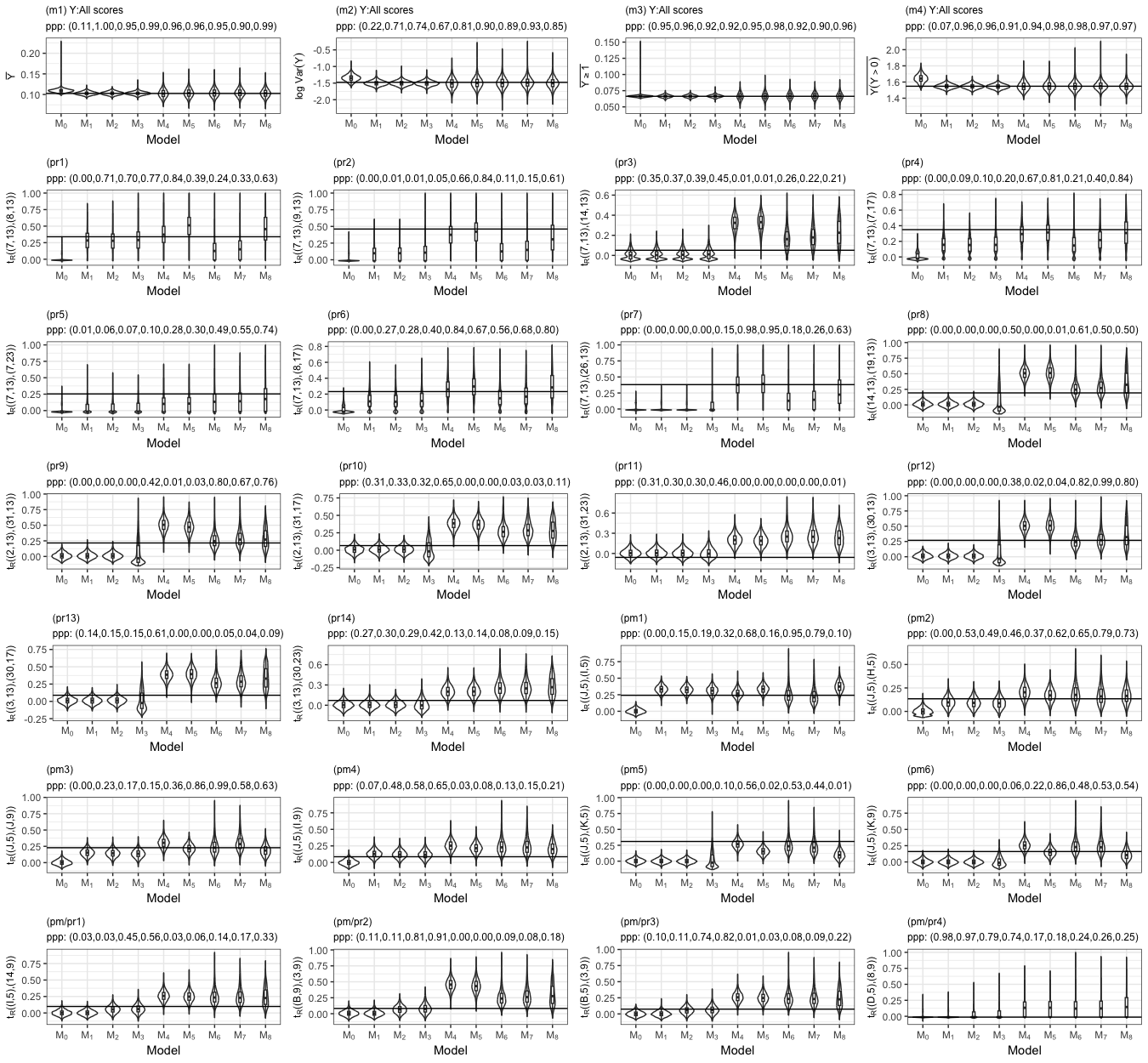
Figure 1: Comparisons of the posterior predictive plots for a subset of ${\boldsymbol{t}}_{M}$ and ${\boldsymbol{t}}_{\bf R}$ elements based on IFS data. The title of each panel shows the $ppp$ values ($ppp=0.00$ indicates $ppp<0.01$) for the corresponding summary statistic obtained from ${\mathcal{M}_{0}}$–${\mathcal{M}_{8}}$. The horizontal line indicates the observed summary statistics.

Figure 1(pr1-pr14) illustrates the predictive distribution of a representative set of correlations between pairs of permanent teeth, while (pm1-pm6) consist of those for primary teeth pairs, and (pm/pr1-pm/pr4) describe the primary-permanent correlation structure. The distributions for all the correlation parameters under model ${\mathcal{M}_{0}}$ are centered around zero, inconsistent with the observed data for many of the considered correlations. Model ${\mathcal{M}_{1}}$, accounting only for temporal and horizontal adjacency, provides a sparse correlation structure as evident from the underestimation in many of predictive distributions. ${\mathcal{M}_{2}}$ accounts for primary-permanent correlation and naturally performs better in (pm/pr1-pm/pr3). Although ${\mathcal{M}_{3}}$ connects all tooth-time pairs, its predictve plots turn out to be very similar to those for ${\mathcal{M}_{2}}$, except having a wider coverage (particularly for vertically adjacent pairs such as pr8 and pr9). This is because $\rho_{v}$ in ${\mathcal{M}_{3}}$ is estimated to be close to zero, leading to similar point estimates of ${\bf R}$, but with greater variability.

While ${\mathcal{M}_{3}}$ provides the model with the most structure, it has poorer fit than ${\mathcal{M}_{4}}$–${\mathcal{M}_{8}}$, which connect tooth-time pairs across space and time more directly through ${\bf W}^{(ct)}$ and ${\bf W}^{(ce)}$. However, we acknowledge that these models provide poor coverage for the IFS data value in a few Spearman correlations (pr11, pr13), where the observed correlations are close to zero, but these cases may not be representative of the full set of correlations for the type of adjacency represented. Overall, the equal connection models ${\mathcal{M}_{6}}$–${\mathcal{M}_{8}}$ appear to perform the best, and we may say that ${\mathcal{M}_{8}}$ is slightly better based on this set of ${\boldsymbol{t}}_{\bf R}$.

Appendix B.3 provides an overall assessment of the model fit for the dependence structure, considering $ppp$ values from all the tooth-time pairs. Combined with the above, this leads us to take ${\mathcal{M}_{8}}$ as the preferred model for the IFS data. While we anticipated that the SAR model combining different spatial relationships based on anatomical consideration (${\mathcal{M}_{3}}$) would best fit the data, it turned out that the dependence model must include an equicorrelation component. As saliva allows food particles and oral bacteria associated with the development of caries to easily travel within the mouth, it is reasonable to conclude that a level of risk is shared across all teeth beyond the associations among adjacent teeth encoded in ${\bf W}^{(h)}$, and this perspective is consistent with the ${\bf W}^{(ce)}$ structure in ${\mathcal{M}_{8}}$.

5.3 IFS Interpretation under the Best Model

We now interpret the best-fitting model ${\mathcal{M}_{8}}$. Coefficient estimates and 95% credible intervals (CI) are shown in Table 2. It is evident from the presence model (1) that the odds of a non-zero caries score decreases as the number of dental visits and the frequency of brushing increases, while the risk of caries increases with higher consumption of sugary beverages. Total daily fluoride ingested does not appear to be associated with the presence of dental caries in this analysis. In the severity model (2), $\beta_{k}$ represents the change in the log-transformed mean caries score for a unit change (one standard deviation) in the $k$-th predictor variable. Table 2 shows that the directions of the behavioral predictor effects are similar to what was seen in the presence model, except for a null effect for brushing.

Predictor		Presence Model			Severity Model
		$\hat{\alpha}$	95% CI		$\hat{\beta}$	95% CI
Intercept		-3.056	(-3.178, -2.934)		-0.879	(-1.015, -0.725)
Dental Visit (past 6 months)		-0.223	(-0.326, -0.115)		-0.186	(-0.296, -0.069)
Daily total fluoride ingested (mgF)		0.007	(-0.079, 0.087)		-0.079	(-0.172, 0.016)
Frequency of brushing (past 6 months)		-0.135	(-0.244, -0.032)		-0.035	(-0.133, 0.063)
Daily total sugar beverage (oz)		0.226	(0.145, 0.301)		0.210	(0.124, 0.287)
Tooth Type
Molar		Ref	–		–	–
Premolar		-0.905	(-0.971, -0.844)		0.138	(0.042, 0.233)
Canine		-0.497	(-0.539, -0.457)		-0.293	(-0.383, -0.213)
Incisor		-0.512	(-0.558, -0.470)		-0.154	(-0.235, -0.073)
Primary		-0.068	(-0.147, 0.017)		0.268	(0.151, 0.384)
Observation Time
Age 5		-0.107	(-0.195, -0.022)		-0.094	(-0.209, 0.012)
Age 9		Ref	–		–	–
Age 13		-0.029	(-0.092, 0.033)		-0.252	(-0.365, -0.135)
Age 17		0.404	(0.341, 0.467)		-0.006	(-0.094, 0.088)
Age 23		0.154	(0.091, 0.222)		0.071	(-0.030, 0.168)
NB size $\phi$					$\hat{\phi}$ = 0.853	(0.722, 1.015)
SAR Parameters		Mean	95% CI
Temporal adjacency ($\rho_{h}$)		0.080	(0.048, 0.103)
Horizontal teeth adjacency ($\rho_{t}$)		0.256	(0.232, 0.278)
Equal connection everywhere ($\rho_{ce}$)		0.0013	(0.0010, 0.0016)

Table 2: Posterior parameter estimates of ${\boldsymbol{\theta}}_{M}$ and ${\boldsymbol{\theta}}_{D}$ for the IFS data under the best-fitting model ${\mathcal{M}_{8}}$.

We further observe that, compared to molar teeth, premolar, canine and incisor teeth are less likely to have a positive caries score, as $\hat{\alpha}_{k}$ are all negative. In the severity model, among those teeth that have a positive caries score, molar teeth also have a higher mean score compared to the incisors and canines. The premolar teeth appear to have significantly higher mean caries score (conditional on having caries) compared to molar teeth, even though they have much lower prevalence. The odds of a non-zero caries score for permanent teeth does not appear to be significantly higher than that for the primary teeth, while for those with positive scores, primary teeth tend to have higher severity. Further, we observe generally increasing odds of caries, with the smallest odds at age 5 and the highest odds at age 17, followed by a small reduction at age 23. Among teeth with caries, the mean score is smaller at 13 than age 9, but there are no other trends among measurement occasions.

The estimation of the SAR model parameters, presented at the bottom of Table 2, shows that both temporal and horizontal adjacency have a statistically significant impact on the dependence structure of the data, and unlike models ${\mathcal{M}_{1}}$–${\mathcal{M}_{3}}$, a significant $\rho_{ce}$ helps maintain non-zero correlations between tooth scores farther away in time or horizontal distance. Estimates of the correlation coefficients ${\boldsymbol{\theta}}_{\bf R}$ are reported in Table B.5.

6 Simulation Studies

We further validate our approach by considering simulation studies similar to the analysis of our IFS data. We imitate the same data structure as the IFS data by generating datasets with the same set of individuals having the same values for the predictors. We consider a Negative Binomial hurdle model for the marginal distributions and the dependence is modeled using the Gaussian copula specified by the SAR model ${\mathcal{M}_{4}}$. This choice assumes all teeth at a given measurement occasion are connected through the adjacency matrix ${\bf W}^{(ct)}$ and imposes autoregressive correlation across time through ${\bf W}^{(t)}$. The data-generating values of all the parameters are similar to the point estimates from the IFS analysis (see Appendix C.1). We generate 100 datasets accordingly, and for each, run three ABC-MCMC chains for 60,000 iterations with $h=0.1,1,10,30$. After regression adjustment, burn-in and thinning, we obtain 9000 posterior samples for each dataset.

We compare estimation of our ABC-MCMC algorithm against ABC rejection and importance samplers (Sisson et al., , 2018, Chapter 1), without and with regression adjustment. See Appendix A.4 for specifics on our implementation of these approaches. These algorithms draw 250,000 samples from the prior and the proposal distributions, respectively, which requires similar computational time as the ABC-MCMC sampler. In our implementation of the rejection algorithm, only 0.1% of the samples closest to ${\boldsymbol{s}}_{\mathrm{obs}}$ are accepted, which is equivalent to having a uniform kernel with data-determined bandwidth.

We assess estimation performance using a range of metrics. Let $\theta_{\cdot;k}$ denote either $\theta_{M;k}$ or $\theta_{{\bf R};k}$, the $k$-th component of ${\boldsymbol{\theta}}_{M}$ or ${\boldsymbol{\theta}}_{\bf R}$, respectively. Let $\hat{\theta}_{\cdot;k,b}$ represent the estimate obtained from the $b$-th simulated data, and $\theta_{\cdot;k,0}$ denote the corresponding true parameter value. Average bias and root mean squared error (RMSE) for each parameter are given by $\frac{1}{B}\sum_{b=1}^{B}(\hat{\theta}_{\cdot;k,b}-\theta_{\cdot;k,0})$ and $\sqrt{\frac{1}{B}\sum_{b=1}^{B}(\hat{\theta}_{\cdot;k,b}-\theta_{\cdot;k,0})^{2}}$, respectively. To investigate posterior coverage, we use a similar strategy as in Uddin and Gaskins, (2023). Letting $(\hat{\theta}_{\cdot;k,b}^{(l_{\zeta})},\hat{\theta}_{\cdot;k,b}^{(u_{\zeta})})$ be a $100\zeta\%$ equal-tailed credible interval, we define the empirical coverage rate (ECR) for parameter $\theta_{\cdot;k}$ as ${\mathrm{ECR}}(\zeta)=\frac{1}{B}\sum_{b=1}^{B}{\bf I}\left(\theta_{\cdot;k,0}\in(\hat{\theta}_{\cdot;k,b}^{(l_{\zeta})},\hat{\theta}_{\cdot;k,b}^{(u_{\zeta})})\right)$. To summarize this coverage, we compute ${\mathrm{ECR}}(\zeta)$ for each $\zeta=0.025,0.050,\ldots,0.975$ and obtain the overall empirical coverage score (${\mathrm{OECS}}$) as the area under the ${\mathrm{ECR}}$ curve (Appendix C.2). An ${\mathrm{OECS}}=0.5$ indicates that the empirical coverage matches the target coverage rate on average, while greater or less than 0.5 indicates over- or under-coverage, respectively. Additionally, to characterize the level of concentration in the estimated posterior distribution, we report the average width of the 80% credible intervals for each parameter.

We use box/violin plots to show the performance on each criterion across all the marginal $({\boldsymbol{\theta}}_{M})$ and correlation $({\boldsymbol{\theta}}_{\bf R})$ parameters. As in the IFS analysis, we include model ${\mathcal{M}_{0}}$ with the independence misspecification and use a Gibbs sampler to fit it. Hence, we treat ${\mathcal{M}_{0}}$ as a baseline and compare the performances of the ABC strategies targeting the true model against it. We only show the results for the importance sampler at bandwidth $h=10$, since this is the $h$ with the best performance of this sampler and of our method. Performance at other bandwidths can be found in Appendix C.2. Also note that the number of unique samples for ABC-MCMC with $h=0.1$ was typically too low to perform regression adjustment, and hence this combination is excluded.

To further summarize differences across the metrics, we compute a ranked order of the accuracy (lowest absolute bias, lowest RMSE, absolute difference between OECS and 0.5) across all methods for each parameter. These ranks are aggregated across the 27 parameters in ${\boldsymbol{\theta}}_{M}$, the 24 parameters in ${\boldsymbol{\theta}}_{\bf R}$, and the 51 parameters in $({\boldsymbol{\theta}}_{M},{\boldsymbol{\theta}}_{\bf R})$ to obtain a consensus ranking of the methods for each metric. Rank aggregation is performed by minimizing the sum of Spearman footrule distances across all parameters (Pihur et al., , 2007, 2008). Additionally, an overall aggregated ranking is found by combining the ranks for all three metrics across parameters (${\boldsymbol{\theta}}_{M}$, ${\boldsymbol{\theta}}_{D}$, or combined). Further details of the rank aggregation approach can be found in Appendix C.1. For the independence model ${\mathcal{M}_{0}}$, we consider all estimates of ${\bf R}({\boldsymbol{\theta}}_{D})$ to be zero, compute OECS based on their credible intervals being $[0,0]$, and exclude consideration of the width of the 80% CI.

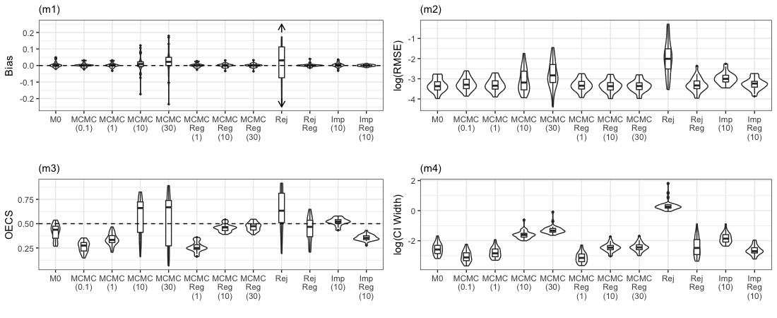
Figure 2: Estimation performance for the marginal parameters ${\boldsymbol{\theta}}_{M}$ from different posterior sampling strategies. In panel (m1), arrows in the boxplot for the ABC rejection indicate truncation, as its tails range from -0.30 to 0.75. All methods except ${\mathcal{M}_{0}}$ are ABC.

In Figure 2(m1), we observe that ${\mathcal{M}_{0}}$ performs fairly well in terms of bias for the marginal parameters. The bias for ABC-MCMC increases with bandwidth. However, post-sampling regression adjustment significantly improves the bias across all the bandwidths and provides competitive performance when compared with ${\mathcal{M}_{0}}$. The ABC rejection sampler performs the worst, with a wide range of bias among the marginal parameters. This is unsurprising as the 0.1% rejection rate selects a (uniform kernel) bandwidth of $h^{*}>20000$, yielding samples of $\Delta({\boldsymbol{s}})$ which are orders of magnitude larger than those from the alternative methods. Noticeable improvement is achieved with regression adjustment. The ABC importance sampler is comparable to that of ABC-MCMC sampler for $h=10$. The first row of Table 3 indicates that ABC importance sampler with regression adjustment performs best, although Figure 2(m1) indicates only slight differences amongst all methods for the criteria (except for rejection and MCMC $h=10,30$).

	${\mathcal{M}_{0}}$	MCMC					MCMC+Reg				Rej	Rej+Reg	Imp	Imp+Reg
$h$		0.1	1	10	30		1	10	30				10	10
Bias
${\boldsymbol{\theta}}_{M}$	6	3	7	10	11		5	8	4		12	2	9	1
${\boldsymbol{\theta}}_{\bf R}$	10	6	4	7	9		1	2	5		12	11	8	3
Combined	10	4	5	7	9		2	1	6		12	11	8	3
RMSE
${\boldsymbol{\theta}}_{M}$	2	7	5	8	11		6	3	1		12	4	10	9
${\boldsymbol{\theta}}_{\bf R}$	10	4	3	6	9		1	2	7		12	11	8	5
Combined	9	6	3	7	11		1	2	4		12	10	8	5
OECS
${\boldsymbol{\theta}}_{M}$	4	10	7	8	11		12	3	2		9	5	1	6
${\boldsymbol{\theta}}_{\bf R}$	12	5	1	6	9		8	2	7		11	10	4	3
Combined	12	8	5	6	9		10	2	3		11	7	1	4
Overall
${\boldsymbol{\theta}}_{M}$	4	10	7	8	11		5	3	1		12	2	9	6
${\boldsymbol{\theta}}_{\bf R}$	10	4	1	6	8		5	2	9		12	11	7	3
Combined	10	5	4	7	9		6	1	2		12	11	8	3

Table 3: Aggregated ranks of the different sampling strategies based on their estimation performance across marginal $({\boldsymbol{\theta}}_{M})$ and correlation $({\boldsymbol{\theta}}_{\bf R})$ parameters. All methods except ${\mathcal{M}_{0}}$ are ABC.

Similar increases in RMSE as $h$ increases are evident in Figure 2(m2). The rejection sampler again performs the worst. Regression adjustment is helpful throughout, and is particularly noticable for the rejection sampler. Parameter estimates from the importance sampler have slightly higher RMSE before regression adjustment (compared to the corresponding MCMC($h=10$)), and after regression adjustment performance is somewhat comparable to the adjusted MCMC (although the aggregate rank is worse). However, the distribution of the importance weights is highly imbalanced; on average, fewer than 15 of 250,000 samples account for more than 50% of the posterior distribution, and hence Imp and Imp+Reg estimation effectively relies on a very small number of posterior samples. MCMC($h=30$) with regression adjustment is the best ranking method in terms of RMSE, followed by ${\mathcal{M}_{0}}$ and MCMC($h=10$) with regression (Table 3).

Turning to Figure 2(m3), we recall that the optimal value for the area under the ECR curve is 0.5. ${\mathcal{M}_{0}}$ frequently undercovers the true parameter values. ABC-MCMC with $h=0.1,1$ yield good point estimates but consistently undercovers, while larger bandwidths ($h=10,30$) overcover. This is further evidenced by Figure 2(m4) with the narrowest CIs for smaller bandwidths and very wide intervals when the bandwidth is larger. This is because ABC-MCMC algorithm with small $h$ is unable to effectively explore the full posterior, since the smaller bandwidth leads to low acceptance rates and small steps. The regression adjustment provides improvement, except under $h=1$ where it exacerbates the issue by further concentrating the posterior. The rejection sampler, with a much wider kernel, results in overcoverage with widest credible intervals. While the unadjusted importance sampler (with poorer point estimation) provided good coverage, Imp+Reg (which had good estimation) undercovers on average. This may be due to the small number of corrected samples getting most of the weights, causing over-shrinkage of the CIs. Overall, Imp($h=10$) and MCMC+Reg($h=10,30$) show acceptable coverage across ${\boldsymbol{\theta}}_{M}$.

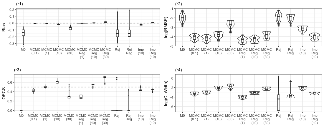
Figure 3: Estimation performance for the correlation parameters ${\boldsymbol{\theta}}_{\bf R}$ from different posterior sampling strategies. All methods except ${\mathcal{M}_{0}}$ are ABC.

Similar plots for the selected correlations are shown in Figure 3. ${\mathcal{M}_{0}}$ assumes ${\bf R}={\bf I}$ and has high bias and poor performance in all metrics. The rejection sampler also has severe bias and estimation error, showing complete failure to learn the dependence structure; regression adjustment provides little help here. This is also reflected by the consistently poor ranks in Table 3. For the ABC-MCMC samplers, the estimation performance deteriorates across all metrics as the bandwidth increases and is more sensitive to $h$ than the marginal parameters. The regression adjustment of the ABC-MCMC samples improves the metrics, with the sampler having the best overall performance at $h=10$.

The last three rows of Table 3 provides the sampler ranks taking all the metrics together. MCMC+Reg($h=30$) is the best with regard to ${\boldsymbol{\theta}}_{M}$ fit, while Rej+Reg and MCMC+Reg($h=10$) are in second and third place. For ${\boldsymbol{\theta}}_{\bf R}$, MCMC($h=1$) performed best combining all the metrics, with MCMC+Reg($h=10$) second best and Imp+Reg($h=10$) in third place. Combing all the performance metrics across all the parameters, MCMC+Reg($h=10$) is found to be the best.

Tables C.7 and C.8 in Appendix C.2 include further details on the bias, RMSE, and coverage for each parameter. In addition to the aforementioned analyses, we conduct some further investigations about the sensitivity of the importance sampler to the bandwidth choice, an alternative regression adjustment approach, and estimation performance under misspecification of the SAR model in Appendices C.2, C.3 and C.4, respectively.

We make some final comments regarding the simulation analysis. In this setting, a bandwidth of $h=10$ appears to strike a balance between good MCMC mixing, while also reducing approximation error associated with the difference between the true posterior (6) and the ABC posterior (7), after regression post-processing. In terms of the aggregated ranks, MCMC+Reg($h=10$) was the only method with good performance (low ranks) for both point estimation and uncertainty quantification. The data structure considered here is similar to that of the IFS data, in terms of the number of observations and the proportion of zero inflation, so these results further validate the choice of $h=10$ in Section 5. For other data settings, the user will need to run ABC-MCMC for multiple bandwidths and determine which $h$ should be used based on similar considerations to those made here.

7 Discussion

In this work, we have proposed a zero-inflated spatio-temporaly correlated count data model. A Negative Binomial hurdle model defines each marginal distribution, facilitating population-level interpretations. A Gaussian copula specifies dependence using a Simultaneous Autoregressive model with multiple adjacency relationships. Standard Bayesian inference is unavailable since the resulting likelihood is intractable, and we employed ABC to estimate an approximate posterior distribution. The posterior samples from ABC-MCMC are further processed using a regression adjustment, and the final adjusted samples are used for inference and validated with posterior predictive checks.

We have employed this model to analyze the Iowa Fluoride Study data. The estimated effects are consistent with conclusions from elsewhere in the dental literature; namely, that low dental visit frequency, low brushing frequency, high soda intake, increased age, and molar tooth type are all risk factors for the appearance and/or severity of caries. Moreover, our approach finds predictor effects at the population-level, unlike Choo-Wosoba et al., (2018); Kang et al., (2021, 2023), where the effects only had individual-level interpretations. The flexibility of our model in specifying the dependence enabled us to fit and compare a variety of potential spatio-temporal correlation structures. The structures based on equal connection choices turned out to be more consistent with the IFS data than structures assuming conditional independencies through spatial structural relationships.

Choosing summary statistics is a critical step in ABC since the model learns only through ${\boldsymbol{s}}({\boldsymbol{y}})$ and not from the likelihood of ${\boldsymbol{y}}$. Our choice of statistics has been motivated through the auxiliary likelihood approach (Drovandi et al., , 2011), where we consider estimates from a simpler model to assess data fit. Posterior predictive checks indicate that our model may struggle with some features of the dependence, requiring more flexible ${\bf R}({\boldsymbol{\theta}}_{D})$ and/or additional parameters in ${\boldsymbol{\theta}}_{D}$. However, this may also be due in part to inadequency of ${\boldsymbol{s}}_{D}({\boldsymbol{Y}})$ for learning ${\boldsymbol{\theta}}_{D}$. Rather than approximating the SAR model, an alternative could directly use the pairwise correlation estimates, similar to how these ${\boldsymbol{t}}_{{\bf R}}({\boldsymbol{y}})$ were used for posterior predictive assessment. There are more than 8,000 such correlations in the IFS data, so some level of dimension reduction would be required. This could potentially be done using entropy-minimizing subset selection (Nunes and Balding, , 2010), projection methods (Fearnhead and Prangle, , 2012), or from an a priori chosen collection.

We have performed model comparison simultaneously with model validation by considering the predictive distributions. Standard model selection for ABC typically involves generating parameters and their corresponding data from the prior under each model and applying a rejection algorithm using summary statistics shared across all models (Fagundes et al., , 2007; Pudlo et al., , 2016). However, as demonstrated in the simulation and IFS examples, approaches like these fail to learn the regions of highest posterior mass and, therefore, will not provide trustworthy estimates of the posterior model probabilities in our context. Other standard Bayesian model selection methods such as DIC (Spiegelhalter et al., , 2002) are not useful here since the likelihood is intractable. Hence, we have opted for model comparison based on intuitive arguments guided by our posterior predictive checks, but further work on ABC model selection methods would be useful in this context.

As noted in Section 3.2, the Gaussian copula facilitates marginalization over the missing data, and ABC generates data ${\boldsymbol{y}}$ with the same missing data pattern as in ${\boldsymbol{y}}_{\mathrm{obs}}$. Thus, we have not required special consideration to account for missingness. In the IFS data, we can consider two sources of missingness. The first is in the spirit of structural missingness (Mitra et al., , 2023) and arises due to the timing of tooth eruption. Unlike analyses specific to high-risk populations (e.g., Jin et al., , 2016), there is no information to be gained by considering which teeth are observed given that the patient is seen at time $t$. Whether an individual tooth is observed is primarily a function of patient age and the transition from primary to permanent teeth, not underlying dental health. More relevant is missingness from whether patients are observed at time $t$. An assumption of auxiliary variable missing at random (Daniels and Hogan, , 2008) is potentially reasonable, as we believe missingness depends not on the unobserved caries score, but on observed predictors such as frequency of dental visits. In that case the missing data mechanism need not be modeled, and our analyses remain valid. We note that our model structure could be easily extended to account for non-ignorable missingness with a selection model approach (Little and Rubin, , 2019). The data generation model $p({\boldsymbol{y}}\mid{\boldsymbol{\theta}})$ would then include the missing data mechanism, and ${\boldsymbol{s}}({\boldsymbol{y}})$ must be adjusted to include statistics related to the missing data indicators. Implementation and investigation of such strategies is beyond the scope of this project.

Appendix A Further Algorithmic Details

In this section, we provide further details of our algorithm and computational strategy that were not included in Section 4 of the main manuscript. Figure A.1 summarizes the full sequence of steps we take to perform parameter estimation. We will first describe our approach to find initial estimates of ${\boldsymbol{\theta}}_{M}$ and ${\boldsymbol{\theta}}_{D}$, along with that for derivation of summary statistics ${\boldsymbol{s}}_{D}({\boldsymbol{Y}})$ and the estimation of kernel scaling matrix ${\bf A}$. The following subsections will present a discussion on the specifics of ABC-MCMC algorithm, including covariance adaptation and hyperparameter ${\boldsymbol{\theta}}_{H}$ sampling. Section A.3 will provide additional details on post-ABC regression adjustment. The final subsection includes details on the ABC rejection and importance sampling algorithms.

Figure A.1: Flow chart of the ABC algorithm. The trapazoid-shaped boxes represent input to the algorithm, rounded-corner boxes are procedures, circles indicate intermediate estimates of parameters and the rightmost box with a double border indicates the final output of the algorithm.

A.1 Initial Estimation

As noted in the main text, our proposed model simplifies to a more tractable model under the assumption ${\boldsymbol{\theta}}_{D}={\mathbf{0}}$. In addition to using this auxiliary likelihood to compute the ABC summary statistics regarding ${\boldsymbol{\theta}}_{M}$, we also use the simplified model to find initial values for our ABC-MCMC algorithm. To that end, we first devised an algorithm for initializing our ABC-MCMC based on estimating ${\boldsymbol{\theta}}_{M}$ conditional on ${\boldsymbol{\theta}}_{D}={\mathbf{0}}$, and then estimating ${\boldsymbol{\theta}}_{D}$ conditional on the estimated ${\boldsymbol{\theta}}_{M}$. The estimation of the initial proposal covariance matrix is also discussed.

As suggested by Pillow and Scott, (2012), we reparameterize the Negative Binomial distribution such that $\phi$, the size parameter, is included in the mean term. Note this reparameterization is only for this step of finding an initial value for ${\boldsymbol{\theta}}_{M}$. The likelihood under ${\boldsymbol{\theta}}_{D}={\mathbf{0}}$ reduces to

$$L^{*}_{\mathrm{ind}}({\boldsymbol{\theta}}_{M}|{\boldsymbol{y}})=\prod\limits_{(i,j)\in\mathcal{D}}\left\{\pi_{ij}\mathbb{I}(y_{ij}=0)+(1-\pi_{ij})p(y_{ij}-1|\phi\exp({\bf x}_{ij}^{\prime}{\boldsymbol{\beta}}),\phi)\mathbb{I}(y_{ij}>0)\right\}.$$ (A.1)

Polson et al., (2013) and Pillow and Scott, (2012) have discussed conjugate Gibbs sampling schemes to obtain posterior samples for logistic and Negative Binomial model parameters, respectively. In both cases, the authors introduced a set of auxiliary variables each following a Pólya-Gamma distribution and expressed binomial and Negative Binomial likelihoods as a mixture of normal distributions with respect to those latent variables. Neelon, (2019) has also used Pólya-Gamma latent variable to implement Gibbs sampling steps for zero-inflated Negative Binomial regression in the context of spatio-temporal analysis. Here, we follow their approaches for the estimation of marginal model parameters ${\boldsymbol{\alpha}}$ and ${\boldsymbol{\beta}}$.

For those $(i,j)\in\mathcal{D}^{*}$, we have $Y_{ij}-1\sim\text{NB}(\mu_{ij}=\phi\exp({\boldsymbol{x}}^{\prime}_{ij}{{\boldsymbol{\beta}}}),\phi)$ with the density,

$$p(y)=\frac{\Gamma(y-1+\phi)}{\Gamma(\phi)(y-1)!}\xi_{ij}^{\phi}(1-\xi_{ij})^{y_{ij}-1},\ \ \xi_{ij}=\frac{1}{(1+\exp({\boldsymbol{x}}_{ij}^{\prime}{\boldsymbol{\beta}}))}.$$

To devise a conjugate sampler for ${\boldsymbol{\beta}}$, we introduce an auxiliary parameter $\omega_{ij}^{({\boldsymbol{\beta}})}$ for each $(i,j)\in\mathcal{D}^{*}$ such that $\omega_{ij}^{({\boldsymbol{\beta}})}|y_{ij},{\boldsymbol{\beta}}\sim\text{PG}(y_{ij}-1+\phi,{\boldsymbol{x}}^{\prime}_{ij}{\boldsymbol{\beta}})$. Using the integral identity (Polson et al., , 2013), we obtain the likelihood contribution to ${\boldsymbol{\beta}}$ from $y_{ij}$ to be

$$L^{*}_{\mathrm{ind}}({\boldsymbol{\beta}}|y_{ij})\propto\frac{\exp({\boldsymbol{x}}^{\prime}_{ij}{{\boldsymbol{\beta}}})^{y_{ij}-1}}{(1+\exp({\boldsymbol{x}}^{\prime}_{ij}{{\boldsymbol{\beta}}}))^{y_{ij}-1+\phi}}\propto e^{\kappa_{ij}({\bf x}^{\prime}_{ij}{\boldsymbol{\beta}})}\int_{0}^{\infty}e^{-\omega^{({\boldsymbol{\beta}})}_{ij}({\bf x}^{\prime}_{ij}{\boldsymbol{\beta}})^{2}/2}p(\omega^{({\boldsymbol{\beta}})}_{ij})d\omega^{({\boldsymbol{\beta}})}_{ij},$$

where $\kappa_{ij}=\frac{1}{2}(y_{ij}-1-\phi)$ and $p(\omega_{ij}^{({\boldsymbol{\beta}})})$ represents the density $\text{PG}(y_{ij}-1+\phi,0)$. We consider $\text{MVN}_{d}({\mathbf{0}},{\boldsymbol{\Sigma}}_{{\boldsymbol{\beta}}})$ as the prior for ${\boldsymbol{\beta}}$ (conditionally on the NG variance parameters). The resulting posterior distribution for ${\boldsymbol{\beta}}$, conditional on the $\omega^{({\boldsymbol{\beta}})}_{ij}$ augmentation parameters, is proportional to

$$e^{-{\boldsymbol{\beta}}^{\prime}{\boldsymbol{\Sigma}}_{{\boldsymbol{\beta}}}^{-1}{\boldsymbol{\beta}}/2}\prod\limits_{(i,j)\in\mathcal{D}}e^{\kappa_{ij}({\bf x}_{ij}^{\prime}{\boldsymbol{\beta}})-\omega({\bf x}_{ij}^{\prime}{\boldsymbol{\beta}})^{2}/2},$$

which is a multivariate normal distribution. The details of the distribution are provided in the following MCMC steps.

To obtain a conjugate sampler for ${\boldsymbol{\alpha}}$, the auxiliary variables $\omega_{ij}^{({\boldsymbol{\alpha}})}$ are introduced, where $\omega_{ij}^{({\boldsymbol{\alpha}})}|z_{ij},{\boldsymbol{\alpha}}\sim\text{PG}(1,{\boldsymbol{x}}^{\prime}_{ij}{\boldsymbol{\alpha}})$. Then the logistic regression model with $\text{logit}(\pi_{ij})=\boldsymbol{x}^{\prime}_{ij}{\boldsymbol{\alpha}}$ as specified in equation (1) implies that the likelihood contribution to ${\boldsymbol{\alpha}}$ from $z_{ij}$ would be

$$L^{*}_{\mathrm{ind}}({\boldsymbol{\alpha}}|z_{ij})\propto\frac{\exp({\boldsymbol{x}}^{\prime}_{ij}{{\boldsymbol{\alpha}}})^{z_{ij}}}{(1+\exp({\boldsymbol{x}}^{\prime}_{ij}{{\boldsymbol{\alpha}}}))}\propto e^{\kappa_{ij}({\bf x}^{\prime}_{ij}{\boldsymbol{\alpha}})}\int_{0}^{\infty}e^{-\omega^{({\boldsymbol{\alpha}})}_{ij}({\bf x}^{\prime}_{ij}{\boldsymbol{\alpha}})^{2}/2}p(\omega^{({\boldsymbol{\alpha}})}_{ij})d\omega^{({\boldsymbol{\alpha}})}_{ij},$$

where $\kappa_{ij}=z_{ij}-1/2$ and $p(\omega^{({\boldsymbol{\alpha}})}_{ij})$ for each $(i,j)\in\mathcal{D}$ is the PG(1,0) density. We choose the prior for ${\boldsymbol{\alpha}}$ to be $\text{MVN}({\mathbf{0}},{\boldsymbol{\Sigma}}_{{\boldsymbol{\alpha}}})$. Due to the conjugate structure resulting from the augmentation of ${\boldsymbol{\omega}}^{({\boldsymbol{\alpha}})}$, we can derive a Gibbs sampling step for sampling ${\boldsymbol{\alpha}}$ from MVN.

Under the independence assumption/misspecification in this auxiliary likelihood, posterior sampling of the parameters for the presence model (${\boldsymbol{\alpha}},{\boldsymbol{\sigma}}_{{\boldsymbol{\alpha}}}^{2},\tau_{{\boldsymbol{\alpha}}}^{2},\lambda_{{\boldsymbol{\alpha}}}$) depends only on $Z_{ij}$, while the severity model parameters (${\boldsymbol{\beta}},{\boldsymbol{\sigma}}_{{\boldsymbol{\beta}}}^{2},\tau_{{\boldsymbol{\beta}}}^{2},\lambda_{{\boldsymbol{\beta}}}$) are only dependent on the non-zero $Y_{ij}$. Since $Z_{ij}$ are known for given data $Y_{ij}$, updating the presence model parameters using the following steps (1a-1c) can be done separately from the steps (2a-2d) for updating the severity model parameters. As such, we can run (1a-1c) and (2a-2d) in parallel to reduce overall computation time. The following sampling steps of the MCMC algorithm are repeated until approximate convergence is achieved.

1. Updating ${{\boldsymbol{\alpha}}}$: We update ${\boldsymbol{\alpha}}$ in two steps: (i) first draw samples for auxiliary variables $\{\omega^{({{\boldsymbol{\alpha}}})}_{ij}\}$ for $i=1,\ldots,n$, $j\in\mathcal{J}_{i}$, $\omega^{({{\boldsymbol{\alpha}}})}_{ij}|{\boldsymbol{\alpha}}\stackrel{{\scriptstyle\text{iid}}}{{\sim}}\text{PG}(1,{\boldsymbol{x}}^{\prime}_{ij}{{\boldsymbol{\alpha}}})$, (ii) then draw ${\boldsymbol{\alpha}}$ as $\left({{\boldsymbol{\alpha}}}|\{\omega^{({{\boldsymbol{\alpha}}})}_{ij}\},\{y_{ij}\}\right)\sim\text{MVN}({\boldsymbol{\mu}}^{*}_{{{\boldsymbol{\alpha}}}},{\boldsymbol{\Sigma}}^{*}_{{\boldsymbol{\alpha}}})$, where ${\boldsymbol{\Sigma}}^{*}_{{\boldsymbol{\alpha}}}=\left(\sum_{i,j}\omega^{({{\boldsymbol{\alpha}}})}_{ij}{\boldsymbol{x}}_{ij}{\boldsymbol{x}}_{ij}^{\prime}+{\boldsymbol{\Sigma}}^{-1}_{{\boldsymbol{\alpha}}}\right)^{-1}$, $\mathbf{\Sigma}_{{\boldsymbol{\alpha}}}=\text{Diag}(\sigma_{\alpha_{0}}^{2},\sigma_{\alpha_{1}}^{2},\ldots,\sigma_{\alpha_{d}}^{2})$ is the prior covariance of ${\boldsymbol{\alpha}}$, and ${\boldsymbol{\mu}}^{*}_{{\boldsymbol{\alpha}}}={\boldsymbol{\Sigma}}^{*}_{{\boldsymbol{\alpha}}}\left(\sum_{i,j}(z_{ij}-1/2){\boldsymbol{x}}_{ij}\right)$.

2. Updating $\boldsymbol{\sigma}^{2}_{{\boldsymbol{\alpha}}}$: The full conditional distribution of $\sigma^{2}_{\alpha_{k}}$ for $k=1,\ldots,d$ is given by the generalized inverse Gaussian (GIG) distribution, $\textrm{GIG}(\lambda_{{\boldsymbol{\alpha}}}-1/2,\alpha_{k}^{2},2\lambda_{{\boldsymbol{\alpha}}}/\tau_{{\boldsymbol{\alpha}}}^{2})$. In this parameterization, the density for $\text{GIG}(x;m,a,b)$ is given by

   $$p(x)=\frac{(a/b)^{m/2}}{2K_{m}(\sqrt{ab})}x^{m-1}\exp\left\{-\frac{1}{2}(ax+b/x)\right\},\ \ \ x>0,$$

   where $K_{m}(\cdot)$ is the modified Bessel function of the second kind.

3. Updating $\tau_{{\boldsymbol{\alpha}}}^{2}$: The full conditional distribution for $\tau_{{\boldsymbol{\alpha}}}^{2}$ is given by $\textrm{IG}(1+d\lambda_{{\boldsymbol{\alpha}}},1+\lambda_{{\boldsymbol{\alpha}}}\sum_{k=1}^{d}\sigma_{\alpha_{k}}^{2})$.

4. Updating ${{\boldsymbol{\beta}}}$: The two steps for updating ${\boldsymbol{\beta}}$ are: (i) first draw samples for auxiliary variables $\{\omega^{({{\boldsymbol{\beta}}})}_{ij}\}_{(i,j)\in\mathcal{D}^{*}}$, $\omega^{({{\boldsymbol{\beta}}})}_{ij}|{\boldsymbol{\beta}}\stackrel{{\scriptstyle\text{iid}}}{{\sim}}\text{PG}(y_{ij}-1+\phi,{\boldsymbol{x}}^{\prime}_{ij}{{\boldsymbol{\beta}}})$, (ii) then draw ${\boldsymbol{\beta}}$ as $\left({{\boldsymbol{\beta}}}|\{\omega^{({{\boldsymbol{\beta}}})}_{ij}\},\{y_{ij}\}\right)\sim\text{MVN}({\boldsymbol{\mu}}_{{{\boldsymbol{\beta}}}}^{*},{\boldsymbol{\Sigma}}^{*}_{{\boldsymbol{\beta}}})$, where

   $${\boldsymbol{\Sigma}}^{*}_{{\boldsymbol{\beta}}}=\left(\sum_{\{i,j:z_{ij}=1\}}\omega^{({{\boldsymbol{\beta}}})}_{ij}{\boldsymbol{x}}_{ij}{\boldsymbol{x}}_{ij}^{\prime}+{\boldsymbol{\Sigma}}^{-1}_{{\boldsymbol{\beta}}}\right)^{-1},\quad{\boldsymbol{\mu}}_{{\boldsymbol{\beta}}}={\boldsymbol{\Sigma}}^{*}_{{\boldsymbol{\beta}}}\left[\sum_{\{i,j:z_{ij}=1\}}\left(\frac{y_{ij}-1-\phi}{2}\right){\boldsymbol{x}}_{ij}\right].$$

   Note that the intercept $\beta_{0}$ is updated in this step along with other $\beta_{k}$, but it will also be updated again in the step (2b) jointly with $\phi$. It is, however, worth mentioning that sampling from the subfamily of $\text{PG}(1,{\boldsymbol{x}}_{ij}^{\prime}{\boldsymbol{\alpha}})$ distributions, as needed for the logistic regression parameters, can be performed very efficiently. However, sampling from $\text{PG}(y_{ij}-1+\phi,{\boldsymbol{x}}_{ij}^{\prime}{\boldsymbol{\beta}})$ for Negative Binomial regression is more challenging and less computationally efficient due to the non-integer shape parameter, as discussed in Polson et al., (2013).

5. Updating $\phi$ and $\beta_{0}$: We update $\beta_{0}$ and $\phi$ jointly in a MH step. Note that $\beta_{0}$ and $\log(\phi)$ are combined to obtain the intercept term in $\log\mu_{ij}=\log\phi+{\boldsymbol{x}}_{ij}^{\prime}{\boldsymbol{\beta}}$ of the Negative Binomial distribution, implying that the value of $\phi$ impacts both $\log(\mu)$ as well as the over-dispersion. Hence, we update $\phi$ by jointly proposing new values for $\beta_{0}$ and $\phi$ in such a way that $\beta_{0}+\log\phi$ (and hence, $\log(\mu_{ij})$) remains unchanged. We generate $\delta$ from symmetric $\mathrm{Unif}[-l,l]$ for some suitable choice of $l>0$ and propose new values of ${\boldsymbol{\beta}}$ and $\phi$ jointly as $\beta_{0}^{*}=\beta_{0}^{(s-1)}+\delta$, $\log\phi^{*}=\log\phi^{(s-1)}-\delta$, and the remaining coefficients are unchanged ($\beta_{k}^{*}=\beta_{k}^{(s-1)}$ for $k=1,\ldots,d$). The probability of acceptance for $({\boldsymbol{\beta}}^{*},\phi^{*}_{0})$ is given by

   $$\min\left\{1,\frac{p({\boldsymbol{\beta}}^{*})p(\log\phi^{*})\prod\limits_{(i,j)\in\mathcal{D}^{*}}p_{\mathrm{NB}}(y_{ij}|\phi^{*}\exp({\boldsymbol{x}}_{ij}^{\prime}{\boldsymbol{\beta}}^{*}),\phi^{*})}{p({\boldsymbol{\beta}}^{(s-1)})p(\log\phi^{(s-1)})\prod\limits_{(i,j)\in\mathcal{D}^{*}}p_{\mathrm{NB}}(y_{ij}|\phi^{(s-1)}\exp({\boldsymbol{x}}_{ij}^{\prime}{\boldsymbol{\beta}}^{(s-1)}),\phi^{(s-1)})}\right\},$$

   where $p_{\mathrm{NB}}$ represents the NB density.

6. Updating $\boldsymbol{\sigma}^{2}_{{\boldsymbol{\beta}}}$: The full conditional distribution of $\sigma^{2}_{\beta_{k}}$ for $k=1,\ldots,d$ is given as $\textrm{GIG}(\lambda_{{\boldsymbol{\beta}}}-1/2,\beta_{k}^{2},2\lambda_{{\boldsymbol{\beta}}}/\tau_{{\boldsymbol{\beta}}}^{2})$.

7. Updating $\tau_{{\boldsymbol{\beta}}}^{2}$: The full conditional distribution for $\tau_{{\boldsymbol{\beta}}}^{2}$ is $\textrm{IG}(1+d\lambda_{{\boldsymbol{\beta}}},1+\lambda_{{\boldsymbol{\beta}}}\sum_{k=1}^{d}\sigma_{\beta_{k}}^{2})$.

We calculate the mean from a large number of posterior samples and denote it as $\widetilde{{\boldsymbol{\theta}}}_{M}$. So that these results correspond to the parameterization in (2), we replace the MCMC sampled $\beta_{0}$ with $\beta_{0}+\log\phi$. This provides our initial estimate for ${\boldsymbol{\theta}}_{M}$. We also obtain the posterior covariance matrix and denote it as $\widetilde{{\boldsymbol{\Sigma}}}_{M}$.

To obtain an initial estimate for ${\boldsymbol{\theta}}_{D}$, denoted as $\widetilde{{\boldsymbol{\theta}}}_{D}$, and a corresponding rough estimate for the covariance matrix denoted as $\widetilde{{\boldsymbol{\Sigma}}}_{D}$, we take the following approach: (a) draw $G=10,000$ samples of ${\boldsymbol{\theta}}_{D}$, represented by $\{{\boldsymbol{\theta}}_{D}^{(g)}\}_{g=1}^{G}$ from a uniform distribution over the subset of the support where each component of ${\boldsymbol{\theta}}_{D}$ is positive; (b) for every ${\boldsymbol{\theta}}^{(g)}=(\widetilde{{\boldsymbol{\theta}}}_{M},{\boldsymbol{\theta}}_{D}^{(g)})$ generate a dataset ${\boldsymbol{y}}^{(g)}$ and a corresponding summary statistic ${\boldsymbol{s}}^{(g)}={\boldsymbol{s}}({\boldsymbol{y}}^{(g)})=({\boldsymbol{s}}_{M}({\boldsymbol{y}}^{(g)}),{\boldsymbol{s}}_{D}({\boldsymbol{y}}^{(g)}))$; (c) select a small set (usually one percent) of the ${\boldsymbol{\theta}}_{D}^{(g)}$ samples for which the Euclidean distances between ${\boldsymbol{s}}_{D}({\boldsymbol{y}}^{(g)})$ and ${\boldsymbol{s}}_{D}({\boldsymbol{y}}_{\text{obs}})$ are smallest, and choose $\widetilde{{\boldsymbol{\theta}}}_{D}$ and $\widetilde{{\boldsymbol{\Sigma}}}_{D}$ as the mean and the covariance matrix of that set of best performing values. The initial estimate of ${\boldsymbol{\theta}}$ is then given as $\widetilde{{\boldsymbol{\theta}}}=(\widetilde{{\boldsymbol{\theta}}}_{M},\widetilde{{\boldsymbol{\theta}}}_{D})$ and the initial covariance matrix for the proposal distribution of ${\boldsymbol{\theta}}$ in the ABC-MCMC algorithm will be block diagonal with components $\widetilde{{\boldsymbol{\Sigma}}}_{M}$ and $\widetilde{{\boldsymbol{\Sigma}}}_{D}$.

We now elaborate on the construction of the summary statistics for ${\boldsymbol{\theta}}_{D}$. First, we obtain naive estimates for the latent Gaussian random variables $V_{ij}$ from the observed data $Y_{ij}$, and then following the SAR model, obtain estimates for the regression coefficients ${\boldsymbol{\theta}}_{D}$ as outlined in Section 4.2. Let $\mathcal{I}_{j}$ denote the subset of individuals who have the $j$-th measurement recorded in the data. We define an empirical CDF for the $j$-th margin, denoted by $\tilde{F}_{j}$ as $\tilde{F}_{j}(y_{ij})=r_{j}(y_{ij})/|\mathcal{I}_{j}|$, where $r_{j}(y)=\sum\limits_{i\in\mathcal{I}_{j}}\mathbb{I}(y_{ij}<y)+\frac{1}{2}\sum\limits_{i\in\mathcal{I}_{j}}\mathbb{I}(y_{ij}=y)$ denotes an estimated rank of $y$ among all the $y_{ij}$ along the $j$-th margin, counting a half contribution for all observations equal to $y$. We set $\widehat{v}_{ij}=\Phi^{-1}(\tilde{F}_{j}(y_{ij}))$. Note that $r_{j}(\cdot)$ is defined such that for any $y_{ij}$ $\widehat{v}_{ij}$ will be set at the median on the restricted range of values of $V_{ij}$ such that $F_{ij}(y_{ij}-1)<\Phi(V_{ij})\leq F_{ij}(y_{ij})$. Additionally, this choice avoids infinite $\hat{v}_{ij}$ for $y=\max_{i\in\mathcal{I}_{j}}y_{ij}$. We further impute $\hat{v}_{ij}=0$ when $y_{ij}$ is missing. The intuition behind this choice is that since a missing $y_{ij}$ can lie anywhere in the support, zero is the median of the corresponding range of $V_{ij}$.

In line with the SAR model in (5), we fit the regression model using these imputed values $\hat{v}_{ij}=\sum_{k=1}^{K}\rho_{k}\widetilde{\raisebox{0.0pt}[0.85pt]{$\widetilde{v}$}}_{ij;k}+\epsilon_{ij}$ for $(i,j)\in\mathcal{D}$, where $\widetilde{\raisebox{0.0pt}[0.85pt]{$\widetilde{v}$}}_{ij;k}=\sum_{j^{\prime}\in\mathcal{J}}w^{(k)}_{jj^{\prime}}\hat{v}_{ij^{\prime}}$. While the variances of $\epsilon_{ij}$ in the SAR model specification differ across $j$, we obtain estimates of $\rho_{1},\ldots,\rho_{K}$ as the regression coefficients in the linear model with an equal variance assumption. The summary statistic vector ${\bf s}_{D}({\bf Y})$ for ${\boldsymbol{\theta}}_{D}$ is given by $(\widetilde{\raisebox{0.0pt}[0.85pt]{$\widetilde{{\bf V}}$}}^{\prime}\widetilde{\raisebox{0.0pt}[0.85pt]{$\widetilde{{\bf V}}$}})^{-1}(\widetilde{\raisebox{0.0pt}[0.85pt]{$\widetilde{{\bf V}}$}}^{\prime}\underaccent{\tilde}{\bsV})$, where $\widetilde{\raisebox{0.0pt}[0.85pt]{$\widetilde{{\bf V}}$}}_{|\mathcal{D}|\times K}=(\widetilde{\raisebox{0.0pt}[0.85pt]{$\widetilde{v}$}}_{ij;k})$ is the latent design matrix and $\underaccent{\tilde}{\bsV}$ is the $|\mathcal{D}|$-dimensional latent outcome vector consisting of $\hat{v}_{ij}$. Note here that we obtain $\widetilde{\raisebox{0.0pt}[0.85pt]{$\widetilde{{\bf V}}$}}$ by stacking the vectors $\widetilde{\raisebox{0.0pt}[0.85pt]{$\widetilde{{\boldsymbol{v}}}$}}_{ij}=(\widetilde{\raisebox{0.0pt}[0.85pt]{$\widetilde{v}$}}_{ij;1},\ldots,\widetilde{\raisebox{0.0pt}[0.85pt]{$\widetilde{v}$}}_{ij;K})$ as rows where $(i,j)\in\mathcal{D}$.

We now turn to kernel estimation strategy. To estimate the kernel scaling matrix denoted by ${\bf A}$, we generate $G=10,000$ sample datasets denoted by $\{{\boldsymbol{y}}^{(g)}\}_{g=1}^{G}$ from $\widetilde{{\boldsymbol{\theta}}}=(\widetilde{{\boldsymbol{\theta}}}_{M},\widetilde{{\boldsymbol{\theta}}}_{D})$, our initial guess at the parameter vector. We compute the sample variance of each summary statistics as $\widetilde{\sigma}^{2}_{k}=\frac{1}{G}\sum_{g=1}^{G}(s^{(g)}_{k}-\bar{s}_{k})^{2}$, where $s^{(g)}_{k}$ is the $k$-th summary statistic of the $g$-th sample ${\boldsymbol{s}}^{(g)}={\boldsymbol{s}}({\boldsymbol{y}}^{(g)})$ and $\bar{s}_{k}=\frac{1}{G}\sum_{g=1}^{G}s^{(g)}_{k}$. We choose ${\bf A}=\textrm{diag}(1/\widetilde{\sigma}^{2}_{1},\ldots,1/\widetilde{\sigma}^{2}_{K})$, where $K$ is the dimension of the vector ${\boldsymbol{s}}^{(g)}$. Note, if $\widetilde{{\boldsymbol{\theta}}}$ is very close to the true value of ${\boldsymbol{\theta}}$, the summary statistics of the generated data $\{{\boldsymbol{s}}^{(g)}\}$ can be considered as a representative sample capturing the covariance structure if we had generated the data based on true ${\boldsymbol{\theta}}$.

A.2 ABC-MCMC Algorithm Specifics

Here we elaborate on certain aspects of the ABC-MCMC algorithm that were not included in the main text due to space constraints. Description of the proposal covariance adaptation scheme is presented. Some details on the posterior sampling of ${\boldsymbol{\theta}}_{H}$ are also provided.

We first discuss the details of the adaptive-MH portion of the ABC-MCMC algorithm, following a strategy from Andrieu and Thoms, (2008, Algorithm 4). Unlike classical Metropolis-Hastings where the random walk covariance matrix is constant, adaptive MCMC allows the covariance in the proposal distribution to change slowly to improve mixing. The proposal density in iteration $g$, denoted by $q_{g}(\cdot|{\boldsymbol{\theta}}^{(g-1)})$, is multivariate normal with mean ${\boldsymbol{\theta}}^{(g-1)}$, the ${\boldsymbol{\theta}}$ sample from iteration $g-1$, and with covariance matrix ${\boldsymbol{\Sigma}}_{g-1}$. The aim here is to adapt the proposal covariance for the next iteration $(g+1)$ taking into account the samples of ${\boldsymbol{\theta}}$ obtained so far, while making sure that the amount of adaptation vanishes fast enough as $g$ increases. At the beginning of the chain (iteration $g=1$), the parameter is initalized at ${\boldsymbol{\theta}}^{(0)}=\widetilde{{\boldsymbol{\theta}}}$ and covariance at ${\boldsymbol{\Sigma}}_{0}=\widetilde{{\boldsymbol{\Sigma}}}$, as described in Section A.1. Let $\overline{{\boldsymbol{\mu}}}_{g}$ and $\overline{{\boldsymbol{\Sigma}}}_{g}$ denote the weighted sample mean and covariance matrix at iteration $g$, which are also initialized at $\widetilde{{\boldsymbol{\theta}}}$ and $\widetilde{{\boldsymbol{\Sigma}}}$. Further, let $\eta_{g}$ be the global covariance scaling factor, initialized at $\eta_{0}=1$.

The covariance adaptation steps in iteration $g$ are performed as part of the acceptance/rejection of the pair $({\boldsymbol{\theta}}^{\prime},{\boldsymbol{y}}^{\prime})$ and include the following steps:

• A value ${\boldsymbol{\theta}}^{\prime}\sim\text{MVN}({\boldsymbol{\theta}}^{(g-1)},{\boldsymbol{\Sigma}}_{g-1})$ is proposed and a decision to accept or reject the sample is made based on the acceptance probability $A\left(({\boldsymbol{\theta}}^{\prime},{\boldsymbol{y}}^{\prime}),({\boldsymbol{\theta}}^{(g-1)},{\boldsymbol{y}}^{(g-1)})\right)$ as discussed in Section 4.3. Let ${\boldsymbol{\theta}}^{(g)}$ denote the final value of the chosen ${\boldsymbol{\theta}}$, which will either be ${\boldsymbol{\theta}}^{(g-1)}$ or ${\boldsymbol{\theta}}^{\prime}$.

• The scaling factor $\eta_{g}$ is updated as

  $$\log\eta_{g}=\log\eta_{g-1}+\nu_{g}\left[A\left(({\boldsymbol{\theta}}^{\prime},{\boldsymbol{y}}^{\prime}),({\boldsymbol{\theta}}^{(g-1)},{\boldsymbol{y}}^{(g-1)})\right)-\bar{p}^{*}_{\text{acc}}\right],$$

  where $\bar{p}^{*}_{\text{acc}}$ represents the target acceptance probability.

• The weighted sample mean and the covariance matrix are updated through

  $$\begin{array}[]{rcl}\overline{{\boldsymbol{\mu}}}_{g}&=&(1-\nu_{g})\overline{{\boldsymbol{\mu}}}_{g-1}+\nu_{g}{\boldsymbol{\theta}}^{(g)},\\ \overline{{\boldsymbol{\Sigma}}}_{g}&=&(1-\nu_{g})\overline{{\boldsymbol{\Sigma}}}_{g-1}+\nu_{g}\left\{({\boldsymbol{\theta}}^{(g)}-\overline{{\boldsymbol{\mu}}}_{g})({\boldsymbol{\theta}}^{(g)}-\overline{{\boldsymbol{\mu}}}_{g})^{\prime}\right\}.\end{array}$$

• The proposal covariance to be used in the next iteration is set to be ${\boldsymbol{\Sigma}}_{g}=\eta_{g}\overline{{\boldsymbol{\Sigma}}}_{g}$.

We choose the vanishing adaptation factor to be $\nu_{g}=1/500$ for the first 500 iterations and $1/g$ for iteration $g>500$. Note that, our choice of $\nu_{g}$ is such that $\sum_{g=1}^{\infty}\nu_{g}=\infty$ ensuring that all the points in the support of ${\boldsymbol{\theta}}$ can be reached, and $\nu_{g}$ also satisfies $\sum_{g=1}^{\infty}\nu_{g}^{2}<\pi^{2}/6<\infty$ implying that the proposed ${\boldsymbol{\theta}}$ samples have bounded fluctuations as discussed in Andrieu and Thoms, (2008).

It is worth making a brief comment on the target acceptance probability $\bar{p}^{*}_{\text{acc}}$. While it is common to specify the target acceptance rate near 0.25, we are generally not able to achieve rates this high since most generated datasets will produce poor kernel values $K_{h}(\Delta({\boldsymbol{s}}))$, driving down the MH probability. So, we must choose a smaller choice for the target acceptance probability $\bar{p}^{*}_{\text{acc}}$ to avoid the proposal variance from collapsing to zero. Here we choose $\bar{p}^{*}_{\text{acc}}=0.1$.

To update the hyperparameters ${\boldsymbol{\theta}}_{H}$ associated with the variance of the regression coefficients, we use classical MH steps to update ${\boldsymbol{\theta}}_{H}$ using two random walk steps for $\log(\tau^{2}_{\alpha})$ and $\log(\tau^{2}_{\beta})$. Here we make use of the fact that the prior on ${\boldsymbol{\alpha}}$ and ${\boldsymbol{\beta}}$ can be marginalized over $\sigma^{2}_{\alpha_{k}}$ and $\sigma^{2}_{\beta_{k}}$, respectively, in closed forms:

$$\begin{array}[]{rcl}\pi(\alpha_{k}|\lambda_{{\boldsymbol{\alpha}}},\tau_{{\boldsymbol{\alpha}}}^{2})&=&\frac{1}{\sqrt{\pi}2^{\lambda_{\alpha}/2-3/4}\Gamma(\lambda_{{\boldsymbol{\alpha}}})}\left(\frac{\lambda_{{\boldsymbol{\alpha}}}}{\tau_{{\boldsymbol{\alpha}}}^{2}}\right)^{\lambda_{{\boldsymbol{\alpha}}}/2+1/4}|\alpha_{k}|^{\lambda_{{\boldsymbol{\alpha}}}-1/2}K_{\lambda_{{\boldsymbol{\alpha}}}-1/2}\left(|\alpha_{k}|\sqrt{\frac{2\lambda_{{\boldsymbol{\alpha}}}}{\tau_{{\boldsymbol{\alpha}}}^{2}}}\right),\\ \pi(\beta_{k}|\lambda_{{\boldsymbol{\beta}}},\tau_{{\boldsymbol{\beta}}}^{2})&=&\frac{1}{\sqrt{\pi}2^{\lambda_{{\boldsymbol{\beta}}}/2-3/4}\Gamma(\lambda_{{\boldsymbol{\beta}}})}\left(\frac{\lambda_{{\boldsymbol{\beta}}}}{\tau_{{\boldsymbol{\beta}}}^{2}}\right)^{\lambda_{{\boldsymbol{\beta}}}/2+1/4}|\beta_{k}|^{\lambda_{{\boldsymbol{\beta}}}-1/2}K_{\lambda_{{\boldsymbol{\beta}}}-1/2}\left(|\beta_{k}|\sqrt{\frac{2\lambda_{{\boldsymbol{\beta}}}}{\tau_{{\boldsymbol{\beta}}}^{2}}}\right).\end{array}$$

The marginalized priors only depend on the hyperparameters $\tau^{2}_{{\boldsymbol{\alpha}}}$ and $\tau^{2}_{{\boldsymbol{\beta}}}$, when $\lambda_{{\boldsymbol{\alpha}}}=\lambda_{{\boldsymbol{\beta}}}=1$. Hence, the full conditional distribution for $\tau_{{\boldsymbol{\alpha}}}^{2}$ and $\tau_{{\boldsymbol{\beta}}}^{2}$ are proportional to $\pi(\tau_{{\boldsymbol{\alpha}}}^{2})\prod_{k=1}^{d}p(\alpha_{k}|\tau_{{\boldsymbol{\alpha}}}^{2})$ and $\pi(\tau_{{\boldsymbol{\beta}}}^{2})\prod_{k=1}^{d}p(\beta_{k}|\tau_{{\boldsymbol{\beta}}}^{2})$, respectively. We choose the proposal distributions $({\tau_{{\boldsymbol{\alpha}}}^{2}}^{*}|\tau_{{\boldsymbol{\alpha}}}^{2})\sim\text{LN}(\tau_{{\boldsymbol{\alpha}}}^{2},\sigma_{\text{MH}}^{2})$ for $\tau_{{\boldsymbol{\alpha}}}^{2}$ and $({\tau_{{\boldsymbol{\beta}}}^{2}}^{*}|\tau_{{\boldsymbol{\beta}}}^{2})\sim\text{LN}(\tau_{{\boldsymbol{\beta}}}^{2},\sigma_{\text{MH}}^{2})$ for proposing $\tau_{{\boldsymbol{\beta}}}^{2}$.

A.3 Regression Adjustment Details

We now elaborate on the regression adjustment procedure. The regression adjustment is typically performed on each univariate component of the parameter vector ${\boldsymbol{\theta}}$, by regressing it with respect to the summary statistics. However, for adjusting a parameter that has a confined support of the form $(l,u)$, where at least one of the bounds is not $\pm\infty$, a suitable transformation is usually advisable. In such cases, the regression correction is performed on the transformed parameter which is then inverse-transformed to obtain the adjusted samples for the parameter. Let $\vartheta$ be a univariate estimand (after transformation when necessary), for instance a component of ${\boldsymbol{\theta}}$ or a more complicated univariate function of ${\boldsymbol{\theta}}$. Our aim is to correct the posterior samples obtained from ABC-MCMC with regression adjustment. We first obtain an estimate of $\textrm{E}(\vartheta|{\boldsymbol{s}})$ at ${\boldsymbol{s}}={\boldsymbol{s}}_{\mathrm{obs}}$ under conditional heteroscedasticity (Blum and François, , 2010), by fitting a local-linear model: $\vartheta^{(g)}=\textrm{E}(\vartheta|{\boldsymbol{s}}^{(g)})+\sigma({\boldsymbol{s}}^{(g)})\epsilon^{(g)}$ to the ABC-MCMC samples, where $\sigma^{2}({\boldsymbol{s}}^{(g)})$ denotes the conditional variance of $\vartheta$ given ${\boldsymbol{s}}={\boldsymbol{s}}^{(g)}$ and $\epsilon^{(g)}$ denotes the standardized residual for the $g$-th sample. The adjusted $\vartheta$ samples, denoted by $\ddot{\vartheta}^{(g)}$, are then computed as $\ddot{\vartheta}^{(g)}=\widehat{\mathrm{E}}(\vartheta|{\boldsymbol{s}}_{\mathrm{obs}})+\hat{\sigma}({\boldsymbol{s}}_{\mathrm{obs}})\hat{\epsilon}^{(g)}$, where the estimated standardized residual $\hat{\epsilon}^{(g)}$ is given by

$$\hat{\epsilon}^{(g)}=\frac{1}{\hat{\sigma}({\boldsymbol{s}}^{(g)})}\left(\vartheta^{(g)}-\widehat{\mathrm{E}}(\vartheta|{\boldsymbol{s}}^{(g)})\right).$$

To perform regression adjustment on a particular correlation coefficients from ${\bf R}({\boldsymbol{\theta}}_{D})$, we note that each correlation is a univariate function of ${\boldsymbol{\theta}}_{D}$ with bounded support $(-1,1)$. For each correlation coefficient $\theta$ of interest, we apply a modified $z$-transform, $\vartheta=z(\theta)=\log\left(\frac{1+\theta}{1-\theta}\right)$, and treat $\vartheta$ as the estimand to be regression-adjusted. The regression-adjusted samples of $\vartheta$, denoted as $\ddot{\vartheta}^{(g)}$, are then inverse-transformed to yield the corresponding samples for $\theta$ given as $\{z^{-1}(\ddot{\vartheta}^{(g)})\}_{g=1}^{G}$. Note that the correlation matrix ${\bf R}$ whose elements have been regression-adjusted individually generally will not give rise to samples of coherent correlation matrices; while each component will be within $(-1,1)$, the joint structure may not be associated with a generator ${\boldsymbol{\theta}}_{D}$ or even be positive definite.

It is worth pointing out here that an alternative implicit adjustment strategy can yield a sample of coherent correlation matrices. Recall that ${\bf R}=({\bf I}-{\bf B})^{-1}{\boldsymbol{\Gamma}}({\bf I}-{\bf B})^{-1}$, where both ${\bf B}$ and ${\boldsymbol{\Gamma}}$ are functions of ${\boldsymbol{\theta}}_{D}$ (see Section 3.3 for details). Therefore, we can first obtain regression-adjusted ABC-MCMC samples of ${\boldsymbol{\theta}}_{D}$, which can be used to generate samples for ${\bf R}$. We consider the strategy of directly adjusting ${\bf R}$ samples as our main approach and compare it with the alternative strategy in Section C.2.

However, adjusting multivariate ${\boldsymbol{\theta}}_{D}$ samples is challenging. Due to the bounded support with multivariate constraints, ${\boldsymbol{\theta}}_{D}$ samples must be transformed before performing adjustment, which in turn is difficult as the support ${\boldsymbol{\Theta}}_{D}$ is not rectangular and does not have a tractable boundary. To that end, we apply the modified $z$-transformation to each component of ${\boldsymbol{\theta}}_{D}^{(g)}$ as if the support for each $\rho_{k}$ were $(-1,1)$. The component-wise transformed ${\boldsymbol{\theta}}_{D}^{(g)}$, denoted by ${\boldsymbol{\vartheta}}_{D}^{(g)}=z({\boldsymbol{\theta}}_{D}^{(g)})$, are regression-adjusted (component-wise) to $\ddot{{\boldsymbol{\vartheta}}}_{D}^{(g)}$ and finally inverse-transformed to obtain the corrected set of samples denoted as $\ddot{{\boldsymbol{\theta}}}_{D}^{(g)}=z^{-1}(\ddot{{\boldsymbol{\vartheta}}}_{D})$. However, this process does not always yield $\ddot{{\boldsymbol{\theta}}}_{D}^{(g)}\in{\boldsymbol{\Theta}}_{D}$, because for the support for transformation space $(-1,1)^{K}$ is a strict superset of parameter space ${\boldsymbol{\Theta}}_{D}$. When the resulting adjusted parameters are outside the correct support $\ddot{{\boldsymbol{\theta}}}_{D}^{(g)}\notin{\boldsymbol{\Theta}}_{D}$, we then believe that $\ddot{{\boldsymbol{\vartheta}}}_{D}^{(g)}$ has been over-corrected, and we need to backtrack toward the original sample vector ${\boldsymbol{\vartheta}}_{D}^{(g)}$ which is generated to lie in ${\boldsymbol{\Theta}}_{D}$. Let ${\boldsymbol{\delta}}=\ddot{{\boldsymbol{\vartheta}}}_{D}^{(g)}-{\boldsymbol{\vartheta}}_{D}^{(g)}$ denote the correction term. Instead of ${\boldsymbol{\delta}}$, we check if correcting ${\boldsymbol{\vartheta}}_{D}^{(g)}$ by ${\boldsymbol{\delta}}/2$ produces a posterior sample in the support, that is, if $\ddot{{\boldsymbol{\theta}}}_{D}^{(g)}=z^{-1}(\ddot{{\boldsymbol{\vartheta}}}_{D}^{(g)})=z^{-1}({\boldsymbol{\vartheta}}_{D}^{(g)}+{\boldsymbol{\delta}}/2)\in{\boldsymbol{\Theta}}_{D}$; if it does not, we further decrease the correction by selecting the first $m=1,2,3,4,5$ such that $z^{-1}({\boldsymbol{\vartheta}}_{D}^{(g)}+{\boldsymbol{\delta}}/2^{m})\in{\boldsymbol{\Theta}}_{D}$. If we still do not get a sample within support with $m=5$, we treat the uncorrected sample ${\boldsymbol{\theta}}_{D}^{(g)}$ as the final corrected version.

A.4 ABC Rejection and Importance Sampling

The standard ABC rejection algorithm is typically very inefficient in high-dimensional settings, and choosing the bandwidth $h$ in a way that balances computational resources and model fit is particularly challenging. In our implementation of the ABC rejection algorithm, we generate and store a large number of parameter vectors ${\boldsymbol{\theta}}^{(g)}$ ($g=1,\ldots,G$), drawn directly from the prior, along with their corresponding data ${\boldsymbol{y}}^{(g)}$ and the summary statistics ${\boldsymbol{s}}^{(g)}$. Finally, we keep 0.1% of the parameter-data pairs that have the smallest $\Delta({\boldsymbol{y}}^{(g)},{\boldsymbol{y}}_{\mathrm{obs}})$; this strategy is roughly equivalent to using the uniform kernel where the bandwidth is given by this percentile of $\Delta({\boldsymbol{y}})$. The samples that are retained are regression-adjusted before using for inference.

We also implement a standard ABC-based importance sampling algorithm. In iteration $g$ of the algorithm, we draw a ${\boldsymbol{\theta}}^{(g)}$ from the proposal density and use it to generate a data ${\boldsymbol{y}}^{(g)}$. The corresponding importance weight is computed as $\tilde{w}^{(g)}\propto K_{h}(\Delta({\boldsymbol{y}}^{(g)},{\boldsymbol{y}}_{\mathrm{obs}}))\pi({\boldsymbol{\theta}}^{(g)})/\tilde{q}({\boldsymbol{\theta}}^{(g)})$, where $\pi(\cdot)$ and $\tilde{q}(\cdot)$ are the prior and the proposal. We run $G$ such proposals, and store the weights along with the parameter-data pairs to be used for inference. The proposal distribution for the importance sampling algorithm is chosen to be a multivariate Normal distribution $\text{MVN}(\widetilde{{\boldsymbol{\theta}}},c^{2}\widetilde{{\boldsymbol{\Sigma}}})$, where $\widetilde{{\boldsymbol{\theta}}}$ and $\widetilde{{\boldsymbol{\Sigma}}}$ are obtained as described in Section A.1. The scaling factor $c^{2}=4$ is chosen to inflate the variance of the proposal distribution in order to propose parameters from a more dispersed distribution than the normal approximation to ${\mathcal{M}_{0}}$. The kernel scaling matrix ${\bf A}$ is the same as what was used for the ABC-MCMC algorithm (see Section A.2). The importance samples are regression-adjusted to obtain the final set of weighted samples.

It is worth adding some comments about the challenges that come with these algorithms. A very large number of parameter draws is required to obtain a set of parameter samples that provides a good approximation to the posterior distribution. This is particularly true in the rejection sampler when drawing directly from a disperse prior. As in ABC-MCMC, the primary computational step is generating the dataset ${\boldsymbol{y}}^{(g)}$ from $p({\boldsymbol{y}}|{\boldsymbol{\theta}})$ and the summarization of the data ${\boldsymbol{s}}({\boldsymbol{y}}^{(g)})$. Consequently, the computational cost of a single iteration is roughly the same for all of these samplers. As ABC-MCMC is best able to propose ${\boldsymbol{\theta}}$ from the region of highest posterior mass, it tends to generate more useful parameter choices and datasets that better match ${\boldsymbol{y}}_{\mathrm{obs}}$. Although regression adjustment was employed on the posterior samples, the correction will only improve estimation if the drawn $({\boldsymbol{\theta}}^{(g)},{\boldsymbol{s}}^{(g)})$ captures the correct relationship locally between the parameters and the summary statistics. But, this does not necessarily happen with rejection sampling since it is using ${\boldsymbol{s}}^{(g)}$s that are very far from ${\boldsymbol{s}}_{\mathrm{obs}}$. In our importance sampling with regression-adjustment, the local regression model is estimated using $({\boldsymbol{\theta}}^{(g)},{\boldsymbol{s}}^{(g)})$ that have approximately zero posterior weight, which may limit the utility of regression adjustment. Further with the importance sampler, the importance sampling weights typically end up highly imbalanced. Different strategies for adjusting the tail of the weight distribution (e.g., Ionides, , 2008; Vehtari et al., , 2022) could be employed to stabilize these weights, but in our experiments, these methods failed to smooth the importance weighted posterior.

Appendix B Additional Details on IFS Data Analysis

In this section, we present additional details on the IFS data analysis presented in Section 5 of the main manuscript. The adjacency matrices defining the dependence model are described in the first subsection, where we explicitly provide all the connections between tooth-time pairs. In Section B.2, we provide a discussion on ABC-MCMC convergence diagnostics. Additional model comparison results are presented next. This section concludes with a discussion on alternative marginal model specifications and assessment of their predictive performance compared to the proposed model.

B.1 Additional model setup details

Figure B.2 provides an overview of the zero-inflation and potential over-dispersion in the IFS data. Additionally, Table B.1 summarizes the IFS data at each age. A brief description of the predictor variables used for the IFS data analysis is contained in Table B.2.

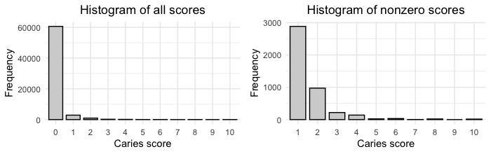
Figure B.2: The figure in the left panel shows the overall distribution of caries experince scores across all teeth, demonstrating clear zero inflation. The figure on the right shows distribution of the non-zero data indicating potential over-dispersion.

Age	Number of	Number of	Proportion	Proportion	Proportion	Proportion	Proportion
	patients	teeth	of $Y=0$	of $Y>0$	of $Y\geq 3$	of $Y\geq 5$	of $Y\geq 8$
all	728	64,926	0.934	0.066	0.007	0.001	0.001
5	696	13,751	0.953	0.047	0.006	0.002	0.001
9	629	14,623	0.948	0.052	0.006	0.001	<0.001
13	549	14,523	0.958	0.042	0.001	0.000	0.000
17	463	12,667	0.881	0.119	0.011	0.001	<0.001
23	342	9362	0.916	0.084	0.013	0.005	0.002

Table B.1: Summary of the caries experience scores in the IFS data categorized by age.

Predictor	Interpretation
Behavioral Variables
Dental Visit (past 6 months)	Proportion of times a dental visit during past 6 months
Daily total fluoride ingested (mgF)	Amount of total fluoride (mg/day) ingested from all sources
Frequency of brushing (past 6 months)	Average daily brushing frequency during past 6 months
Daily amount of sugar beverages (oz)	Amount of total sugar-added beverages consumed (oz/day)
Tooth Type	(see Figure B.3)
Molar	Reference category
	(primary: A,B,I,J,K,L,S,T; permanent: 1-3,14-16,17-19,30-32)
Pre-molar	Indicator variable for pre-molar teeth
	(permanent: 4,5,12,13,20,21,28,29)
Canine	Indicator variable for canine teeth
	(primary: C,H,M,R; permanent: 6,11,23,27)
Incisor	Indicator variable for incisor teeth
	(primary: D,E,F,G,N,O,P,Q; permanent: 7,8,9,10,23,24,25,26)
Primary	Indicator variable to distinguish primary teeth from
	permanent teeth (primary: 1, permanent: 0)
Observation Time
Age-5	Indicator variable for age 5
Age-9	Reference category
Age-13	Indicator variable for age 13
Age-17	Indicator variable for age 17
Age-23	Indicator variable for age 23

Table B.2: Description of the predictors for the IFS data.

We now enumerate the adjacency relationships we considered for modeling the dependence structure of the IFS data.

${\bf W}^{(t)}$: Temporal adjacency
For each location $l\in\{1,\ldots,32\}\cup\{A,\ldots,T\}$
$((l,5),(l,9))$	$((l,9),(l,13))$	$((l,13),(l,17))$	$((l,17),(l,23))$
${\bf W}^{(h)}$: Horizontal tooth adjacency
For each time $t\in\{5,9,13,17,23\}$, connected pairs are:
((1,$t$),(2,$t$))	((2,$t$),(3,$t$))	((3,$t$),(4,$t$))	((4,$t$),(5,$t$))	((5,$t$),(6,$t$))
((6,$t$),(7,$t$))	((7,$t$),(8,$t$))	((8,$t$),(9,$t$))	((9,$t$),(10,$t$))	((10,$t$),(11,$t$))
((11,$t$),(12,$t$))	((12,$t$),(13,$t$))	((13,$t$),(14,$t$))	((14,$t$),(15,$t$))	((15,$t$),(16,$t$))
((16,$t$),(17,$t$))	((17,$t$),(18,$t$))	((18,$t$),(19,$t$))	((19,$t$),(20,$t$))	((20,$t$),(21,$t$))
((21,$t$),(22,$t$))	((22,$t$),(23,$t$))	((23,$t$),(24,$t$))	((24,$t$),(25,$t$))	((25,$t$),(26,$t$))
((26,$t$),(27,$t$))	((27,$t$),(28,$t$))	((28,$t$),(29,$t$))	((29,$t$),(30,$t$))	((30,$t$),(31,$t$))
((31,$t$),(32,$t$))
((A,$t$),(B,$t$))	((B,$t$),(C,$t$))	((C,$t$),(D,$t$))	((D,$t$),(E,$t$))	((E,$t$),(F,$t$))
((F,$t$),(G,$t$))	((G,$t$),(H,$t$))	((H,$t$),(I,$t$))	((I,$t$),(J,$t$))	((K,$t$),(L,$t$))
((L,$t$),(M,$t$))	((M,$t$),(N,$t$))	((N,$t$),(O,$t$))	((O,$t$),(P,$t$))	((P,$t$),(Q,$t$))
((Q,$t$),(R,$t$))	((R,$t$),(S,$t$))	((S,$t$),(T,$t$))
${\bf W}^{(v)}$: Vertical tooth adjacency
For each time $t\in\{5,9,13,17,23\}$, connected pairs are:
((1,$t$),(32,$t$))	((2,$t$),(31,$t$))	((3,$t$),(30,$t$))	((4,$t$),(29,$t$))	((5,$t$),(28,$t$))
((6,$t$),(27,$t$))	((7,$t$),(26,$t$))	((8,$t$),(25,$t$))	((9,$t$),(24,$t$))	((10,$t$),(23,$t$))
((11,$t$),(22,$t$))	((12,$t$),(21,$t$))	((13,$t$),(20,$t$))	((14,$t$),(19,$t$))	((15,$t$),(18,$t$))
((16,$t$),(17,$t$))
((A,$t$),(T,$t$))	((B,$t$),(S,$t$))	((C,$t$),(R,$t$))	((D,$t$),(Q,$t$))	((E,$t$),(P,$t$))
((F,$t$),(O,$t$))	((G,$t$),(N,$t$))	((H,$t$),(M,$t$))	((I,$t$),(L,$t$))	((J,$t$),(K,$t$))
${\bf W}^{(pp)}$: Primary-permanent adjacency
For each time $t_{k}\in\{5,9,13,17,23\}$, with $t_{k}$ and $t_{k+1}$ being adjacent time points, connected pairs are:
((2,$t_{k}$),(A,$t_{k+1}$))	((8,$t_{k}$),(E,$t_{k+1}$))	((14,$t_{k}$),(I,$t_{k+1}$))	((22,$t_{k}$),(M,$t_{k+1}$))	((26,$t_{k}$),(Q,$t_{k+1}$))
((3,$t_{k}$),(B,$t_{k+1}$))	((9,$t_{k}$),(F,$t_{k+1}$))	((15,$t_{k}$),(J,$t_{k+1}$))	((23,$t_{k}$),(N,$t_{k+1}$))	((27,$t_{k}$),(R,$t_{k+1}$))
((6,$t_{k}$),(C,$t_{k+1}$))	((10,$t_{k}$),(G,$t_{k+1}$))	((18,$t_{k}$),(K,$t_{k+1}$))	((24,$t_{k}$),(O,$t_{k+1}$))	((30,$t_{k}$),(S,$t_{k+1}$))
((7,$t_{k}$),(D,$t_{k+1}$))	((11,$t_{k}$),(H,$t_{k+1}$))	((19,$t_{k}$),(L,$t_{k+1}$))	((25,$t_{k}$),(P,$t_{k+1}$))	((31,$t_{k}$),(T,$t_{k+1}$))
${\bf W}^{(ct)}$: Equal connection across location within same time
For each location $l_{1},l_{2}\in\{1,\ldots,32\}\cup\{A,\ldots,T\}$ and $t\in\{5,9,13,17,23\}$, connected pairs are:
$((l_{1},t),(l_{2},t))$
${\bf W}^{(ce)}$: Equal connection everywhere (across location and time)
For each location $l_{1},l_{2}\in\{1,\ldots,32\}\cup\{A,\ldots,T\}$ and $t_{1},t_{2}\in\{5,9,13,17,23\}$, connected pairs are:
$((l_{1},t_{1}),(l_{2},t_{2}))$

Table B.3: Adjacency relationships used in the IFS analysis.

Table B.3 presents all the tooth-time pairs that are adjacent according to the proximity relations in the matrices ${\bf W}^{(t)}$, ${\bf W}^{(h)}$, ${\bf W}^{(v)}$, ${\bf W}^{(pp)}$, ${\bf W}^{(ct)}$ and ${\bf W}^{(ce)}$. To recall, we have five time-points in the data, based on the measurement ages of 5, 9, 13, 17 and 23. There are 20 primary tooth locations denoted by letters A, B, $\ldots$, T and the 32 permanent tooth locations are numbered 1,2, $\ldots$, 32. For reference, we include a pictorial representation in Figure B.3 of the standard naming convention for tooth locations inside mouth.

Figure B.3: The mixed dentition chart shows all the primary and permanent teeth with the approximate age of eruption.

B.2 ABC-MCMC Mixing and Convergence

For each model, we have run 3 chains of ABC-MCMC, each of length 185,000, from which the first 5000 from each chain were removed as the burn-in phase. We have considered four bandwidth choices of 1, 10, 30 and 100 for the IFS data analysis. While these samples are regression-adjusted to yield the final set of approximate posterior samples for inference, here we first discuss the performance and mixing of the ABC-MCMC algorithm with regard to the pre-adjustment samples.

Models	Dependence Structure	$h=1$	$h=10$	$h=30$	$h=100$
${\mathcal{M}_{1}}$	${\bf B}=\rho_{t}{\bf W}^{(t)}+\rho_{h}{\bf W}^{(h)}$	0.22	0.92	1.06	1.11
${\mathcal{M}_{2}}$	${\bf B}=\rho_{t}{\bf W}^{(t)}+\rho_{h}{\bf W}^{(h)}+\rho_{pp}{\bf W}^{(pp)}$	0.15	0.90	1.04	1.29
${\mathcal{M}_{3}}$	${\bf B}=\rho_{t}{\bf W}^{(t)}+\rho_{h}{\bf W}^{(h)}+\rho_{pp}{\bf W}^{(pp)}+\rho_{v}{\bf W}^{(v)}$	0.13	0.83	1.04	1.36
${\mathcal{M}_{4}}$	${\bf B}=\rho_{ct}{\bf W}^{(ct)}+\rho_{t}{\bf W}^{(t)}$	0.03	0.76	0.91	1.15
${\mathcal{M}_{5}}$	${\bf B}=\rho_{ct}{\bf W}^{(ct)}+\rho_{t}{\bf W}^{(t)}+\rho_{h}{\bf W}^{(h)}$	0.02	0.76	0.86	1.20
${\mathcal{M}_{6}}$	${\bf B}=\rho_{ce}{\bf W}^{(ce)}$	0.04	0.71	1.01	1.25
${\mathcal{M}_{7}}$	${\bf B}=\rho_{ce}{\bf W}^{(ce)}+\rho_{t}{\bf W}^{(t)}$	0.04	0.74	0.99	1.17
${\mathcal{M}_{8}}$	${\bf B}=\rho_{ce}{\bf W}^{(ce)}+\rho_{t}{\bf W}^{(t)}+\rho_{h}{\bf W}^{(h)}$	0.09	0.77	1.20	1.17

Table B.4: Acceptance rate per 100 ABC-MCMC samples across different models and bandwidth choices for the IFS analysis.

Table B.4 reports the MH acceptance rate across different bandwidths and models. Since the ABC-MCMC algorithm accepts or rejects the parameter and the generated dataset jointly, the acceptance rate is low compared to standard Metropolis algorithms. As expected when the bandwidth increases, so does the percentages of accepted samples for each model. This is because higher bandwidth allows more disagreement between the proposed ${\boldsymbol{s}}$ and the observed ${\boldsymbol{s}}_{\mathrm{obs}}$. While we may wish to use $h=1$, since smaller $h$ means that $\pi_{\mathrm{ABC}}({\boldsymbol{\theta}}\,|\,{\boldsymbol{s}}_{\mathrm{obs}})$ in equation (7) is closer to the target posterior $\pi({\boldsymbol{\theta}}\,|\,{\boldsymbol{y}}_{\mathrm{obs}})$ in (6), we get much poorer computational performance with this small bandwidth, yielding very few unique samples during ABC-MCMC. This indicates that the ABC algorithm has failed to move around the parameter space effectively and is potentially stuck at a local mode. Under $h=10$ we get a manageable acceptance rate, which does not increase considerably as the bandwidth increases from $h=10$ to $h=100$. Therefore, we consider at least $h=10$ in this case.

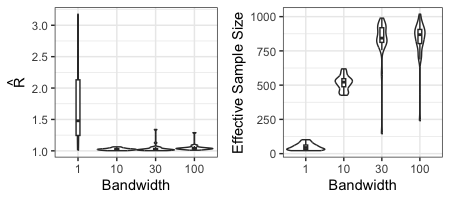
Figure B.4: Boxplots with $\hat{R}$ and effective sample sizes for all the parameters across different bandwidth choices under the selected model ${\mathcal{M}_{8}}$.

We compare the MCMC convergence and mixing across different bandwidth choices in Figure B.4. To generate the plots, we combine the samples from all the chains (without thinning) and obtain a total sample size of 540,000. For each choice of $h$, we compute the Gelman-Rubin $\hat{R}$ statistic for all the parameters and create a boxplot in the left panel of Figure B.4. These comparisions are based on the selected model ${\mathcal{M}_{8}}$, although results are qualitatively similar when comparing within other model choices. We observe poor convergence for most of the parameters when $h=1$ with $\hat{R}>1.1$ for almost all parameters. Convergence is much better in the case of $h=10$, as also shown in the trace plots in Figures B.5–B.6. Mixing for the larger bandwidths is also generally good.

The effective sample sizes (ESS) also portray a similar picture in the right panel of Figure B.4. We calculate the ESS for each MCMC chain using the standard definition $N/(1+\sum_{t=1}^{\infty}\varrho_{t})$, where $N$ is the chain length and $\varrho_{t}$ represents the estimated autocorrelation at lag $t$ for the chain. The combined ESS is found by summarizing across the three MCMC chains. Average ESS across all parameters grows as $h$ increases from 1 to 30, but does not increase further when $h=100$. Additionally, the range of ESS across the different parameters is quite wide at $h=30$ and 100. This suggests that, for larger $h$, ABC-MCMC is not moving as efficiently in some directions of the joint parameter space. This indicates that increasing the bandwidth, thereby allowing the sampler to accept ${\boldsymbol{s}}$ that differ more from ${\boldsymbol{s}}_{\mathrm{obs}}$, beyond a certain threshold has not helped increase the effective sample size. Moreover, with larger $h$ we allow for more approximation error in the ABC posterior. These observations indicates that $h=10$ is an effective choice.

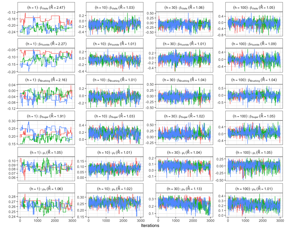
Figure B.5: Comparisons of the mixing of the ABC-MCMC chains from model ${\mathcal{M}_{8}}$ for few selected parameters under different bandwidth choices. The retained values (pre-adjustment) after thinning are depicted in different colors (red, green, blue) for each chain.

We investigate the MCMC mixing/convergence for a subset of parameters in Figure B.5, where each column represents the MCMC chains corresponding to a bandwidth choice. As noted previously, we run three chains for each method, and these traceplots depict the samples from each chain in different color, after thinning to 3000 samples per chain. It is very clear that the ${\boldsymbol{\beta}}$ parameters do not mix well when $h=1$, with $\hat{R}$ values around 2. For the other bandwidths, convergence appears to be achieved and mixing is acceptable. As $h=10$ is the smallest bandwidth considered that has acceptable computational performance, this is the choice we use for inference of the IFS data.

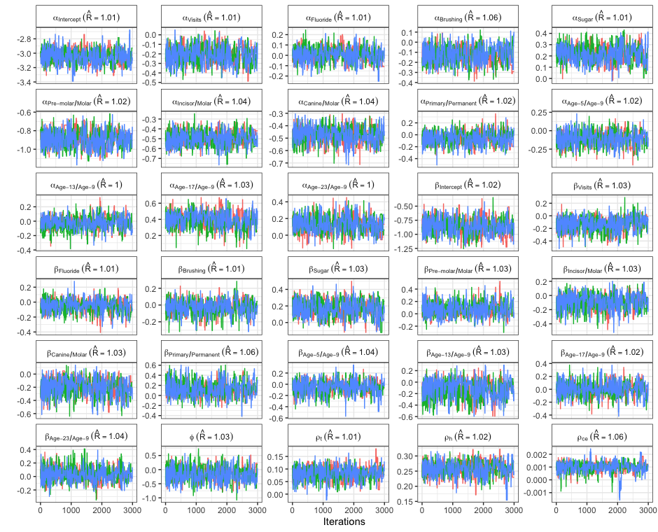
Figure B.6: Mixing of the ABC-MCMC chains ($h=10$) for different parameters under model ${\mathcal{M}_{8}}$. The retained values (pre-adjustment) after thinning for each chain are depicted in different colors (red, green, blue).

Having chosen $h=10$ as the bandwidth for analysis, we now create trace plots from the ABC-MCMC chains for all model parameters ${\boldsymbol{\theta}}$ in Figure B.6 to ensure no other diagnostic concerns. The chains appear to have good mixing and to have reached convergence as reflected by the Gelman-Rubin statistic ($\hat{R}<1.1$ for each parameter). Note that we achieve fairly good convergence for the severity model parameters ${\boldsymbol{\beta}}$ and $\phi$, despite having much smaller amounts of data available to fit the severity model due to zero-inflation.

We would also like to further comment on the applicability of the importance sampler for analysis of the IFS data. The importance sampling strategy (Appendix A.4) was employed to generate $G$=1,200,000 posterior samples of ${\boldsymbol{\theta}}$ and their corresponding weights for the same bandwidth choices ($h=1,10,30,100$). Generating 1.2 million samples required approximately double the computing time as was required for running the corresponding ABC-MCMC. The importance weights were highly imbalanced regardless of the bandwidth used; with the largest $h=100$, the top five weights turned out to be 0.23, 0.19, 0.17, 0.06 and 0.05, accounting for more 70% of the posterior distribution. The posterior was even more tightly concentrated on a handful of samples for the other bandwidths. Pareto smoothing the importance weights (Vehtari et al., (2022)) was not useful, as the Pareto $\hat{k}$ diagnostics were more 1, indicating that a reliable finite variance point estimate can not be obtained. Hence, we can not pursue any further interpretation of the IFS analysis under an ABC importance sampling estimation strategy. While not included here, additional experiments using a sequential Monte Carlo (SMC) algorithm and its extensions for ABC (Sisson et al., , 2007; Bonassi and West, , 2015) also failed to achieve balanced weights in our experiments.

We also investigated the performance of the proposed ABC-MCMC algorithm under a uniform kernel. When using a uniform kernel rather than the Gaussian kernel, we find that the initial parameter value is a more important choice to ensure MCMC mixing. For one, we must initialize using a dataset ${\boldsymbol{y}}$ such that $\Delta({\boldsymbol{s}})<h$, otherwise the joint likelihood is not defined. But, finding a ${\boldsymbol{\theta}}^{(0)}$ that yields such a ${\boldsymbol{y}}$ may require hundreds or thousands of draws from $p({\boldsymbol{y}}|{\boldsymbol{\theta}})$ when $h$ is small. Even after finding an initial value, it will continue to be rare to generate a proposed ${\boldsymbol{y}}$ with $\Delta({\boldsymbol{s}})<h$ as the chain runs. Alternatively, using a large $h$ can facilitate accepting new data, this tended to lead to high autocorrelation in the posterior samples ${\boldsymbol{\theta}}$. While this can be corrected through careful tuning of the adaptive MH parameters, we find that running ABC-MCMC with the uniform kernel is more sensitive to algorithmic choices such as the initial data and parameter values and the adaptation parameters $\eta_{0}$ and $(\nu_{g})$. Consequently, we recommend the Gaussian kernel and limit our analyses to this choice.

B.3 Additional Model Comparison Results for the IFS Data

We now present additional model comparison results for the IFS data. First, we present the full set of posterior predictive plots for assessing the marginal model fit in Figure B.7. In addition to the overall mean and variance of $Y$, we consider $\overline{Y\geq k}$ denoting proportion of $Y\geq k$ for different choices of $k$, we let $\overline{Y(Y\geq k)}$ be the mean of $Y$ over those $Y\geq k$, and $\textrm{Var}(Y(Y\geq k))$ indicates the variance of $Y$ restricted to $Y\geq k$. In particular, we choose $k=8$ to evaluate the predictive ability of the model in the tail of the $Y$ distribution. Moreover, for different predictors $X$, we considered statistics of the form $\overline{Y(X\leq X_{1/3})}-\overline{Y(X>X_{2/3})}$, that captures the difference between the mean of $Y$ corresponding to observations where the predictor value is less than or equal to its first tertile $X_{1/3}$ and those with $X$ is above its second tertile $X_{2/3}$. This will inform if the model is capturing the association between $X$ with $Y$. When $X$ is binary, such as, if the predictor is the indicator of premolar tooth, the statistic will be the mean difference between the caries scores among all premolar teeth to the mean score of other tooth types.

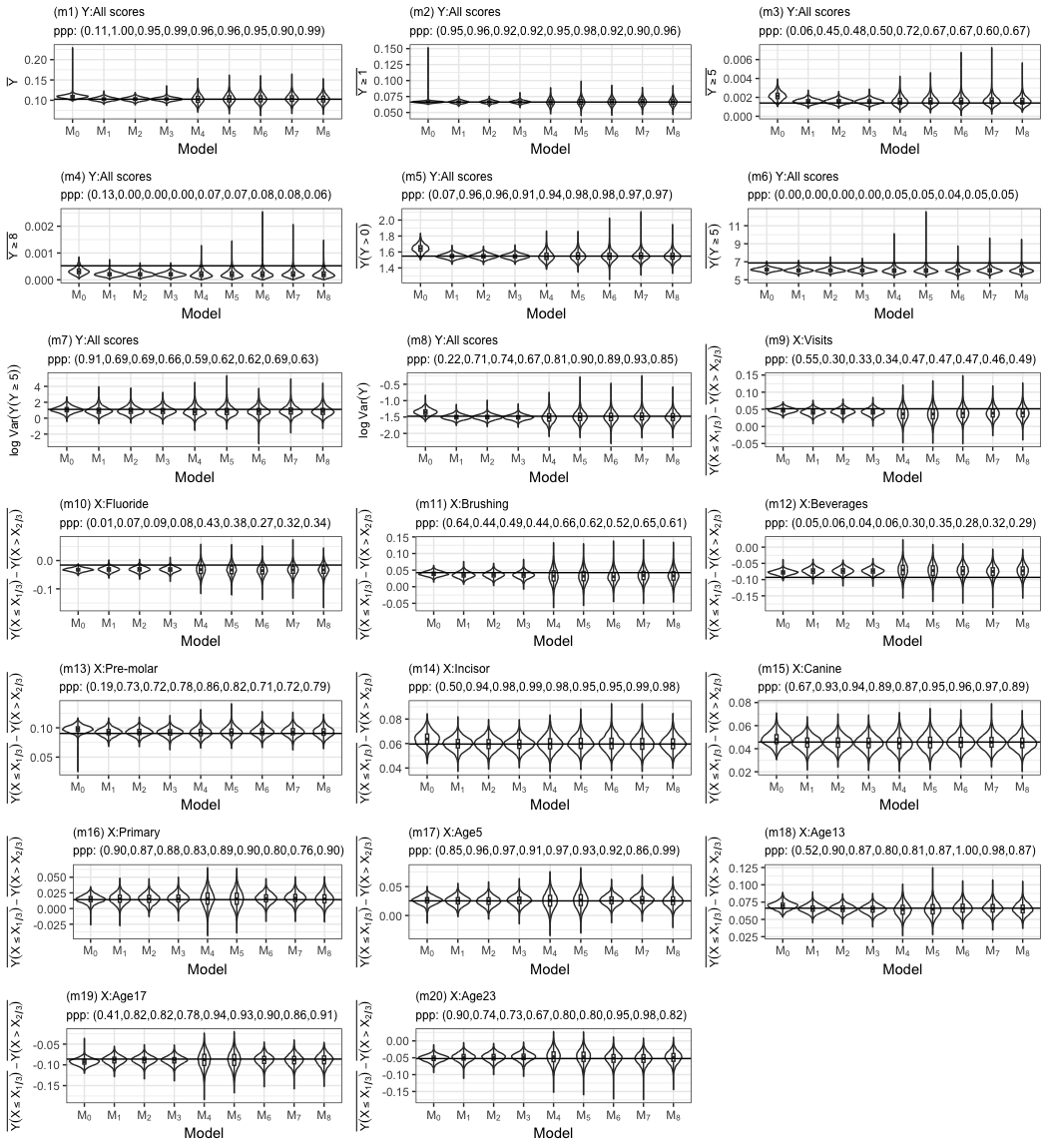
Figure B.7: Comparisons of the posterior predictive plots for ${\boldsymbol{t}}_{M}$ from different models based on IFS data. The title of each plot shows the $ppp$ values ($ppp=0.00$ indicates $ppp<0.01$) for the corresponding summary statistic obtained from ${\mathcal{M}_{0}}$–${\mathcal{M}_{8}}$ consecutively and the horizontal line indicates the observed summary statistics.

As summarized in the main manuscript, we observe from panels (m1)–(m20) that the SAR models ${\mathcal{M}_{1}}$–${\mathcal{M}_{8}}$ have comparable performance. Model ${\mathcal{M}_{0}}$ with its independence misspecification does not account for the correlation present in the data and results in overestimation of the overall mean (m1) and the mean of the non-zero counts (m5). None of the models could explain the larger counts very well (see Figure B.7(m4,m6)). This is potentially due to the fact that the largest count score available in IFS data is 10, with much smaller frequencies for the counts $\geq 8$ compared to that for zeros. Models ${\mathcal{M}_{4}}$–${\mathcal{M}_{8}}$, however, performed better in this regard compared to ${\mathcal{M}_{1}}$–${\mathcal{M}_{3}}$. They also performed better when characterizing the covariate effects on the count scores. For example, the effect of total fluoride consumption is underestimated (m10) by ${\mathcal{M}_{0}}$–${\mathcal{M}_{3}}$, while that of the sugary beverage is overestimated (m12). It is important to note here that ${\mathcal{M}_{4}}$–${\mathcal{M}_{8}}$ have wider predictive distributions compared to the rest, as the dependence structure for the former models include the overall connectivity relationships ${\bf W}^{(ct)}$ and ${\bf W}^{(ce)}$, these assume higher amounts of correlation (less information from the data) than ${\mathcal{M}_{1}}$–${\mathcal{M}_{3}}$ with their sparser connectivity.

To compare parameter estimation of ${\boldsymbol{\theta}}_{M}$ across the different models, we turn to Figure B.9 that displays the posterior mean and 95% credible interval under each model choice for each of the parameters in the logistic prevalence model. We observe that model ${\mathcal{M}_{0}}$ has the narrowest credible intervals throughout. Recall that model fit for ${\mathcal{M}_{0}}$ was performed using a Gibbs sampler targeting the exact posterior, under the independence misspecfication. The point estimate for ${\boldsymbol{\alpha}}$ does not seem to be sensitive to the misspecified dependence structure, while the uncertainty does vary across models. Models ${\mathcal{M}_{1}}$–${\mathcal{M}_{3}}$ specify more structured dependence (see Table 1), while models ${\mathcal{M}_{4}}$–${\mathcal{M}_{8}}$ directly provide an overall connectivity. Hence, consistent with the variability in the prediction distributions, many parameters in ${\boldsymbol{\alpha}}$ have wider credible intervals for these less structured SAR models.

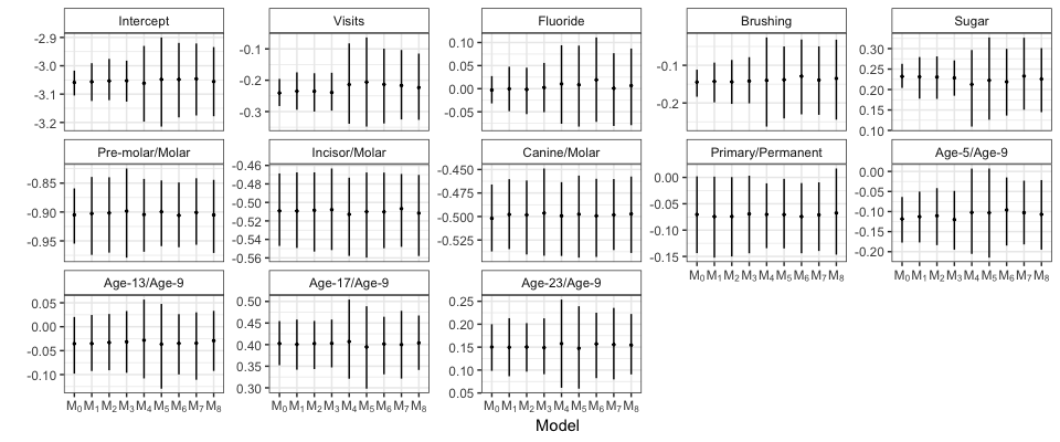
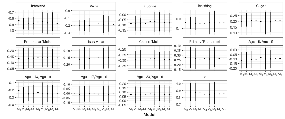
Figure B.8: Comparisons of the regression-adjusted ${\boldsymbol{\alpha}}$ estimates from different models. The point estimate for each model is denoted by the dot, while the line shows the 95% confidence interval.

Figure B.9: Comparisons of the regression-adjusted ${\boldsymbol{\beta}}$ and $\phi$ estimates from different models. The point estimate for each model is denoted by the dot, while the line shows the 95% confidence interval.

We observe similar behavior in the NB parameters as well, as shown in Figure B.9. The point estimates for ${\boldsymbol{\beta}}$ are more sensitive to the independence misspecification than the ${\boldsymbol{\alpha}}$ parameter; in particular the estimates for the tooth indicator “Canine/Molar” and time indicator “Age-13/Age-9” differ for model ${\mathcal{M}_{0}}$ compared to the rest of the models.

Overall, hese results show relatively minimal differences in the models for the marginal parameters consistent with the posterior predictive plots in Figure B.7. However, we saw more meaningful differences in the posterior predictive plots of the selected 24 Spearman correlations (Figure 1 of main manuscript). To complement these comparisons and further investigate the much larger collection of correlations that our model specifies, we consider the univariate $ppp$ values for a larger number of correlations (instead of the full predictive distribution for a small number of correlations). For each model, we compute the corresponding $ppp$ values of the Spearman correlation of all pairs $(l_{j},t_{j})$ and $(l_{j^{\prime}},t_{j^{\prime}})$ and plot the histogram across these $ppp$s. Note that we include only those $ppp$ values which correspond to correlation coefficients obtained from at least 100 pairs of caries scores. While looking into the posterior predictive distributions for a few representative elements from ${\bf R}$ as in Figure 1 helps identify those specific features of the dependence model that are being mis-modeled, considering the histogram consisting of all $ppp$ values provides a more holistic view into the model fit.

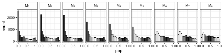
Figure B.10: Histogram of all available $ppp$-values across all model choices.

As shown in Figure B.10, the histogram for ${\mathcal{M}_{0}}$ has a very high peak near zero, implying that the posterior predictive distributions of a large number of Spearman correlations poorly represent the corresponding values observed in the IFS data. This is also observed in most of the alternative model choices based on the anatomic SAR models ${\mathcal{M}_{1}}$–${\mathcal{M}_{3}}$ and to a lesser extent the equal connection within time based ${\mathcal{M}_{4}}$ and ${\mathcal{M}_{5}}$. The models with ${\bf W}^{(ce)}$ included have the best performance and mostly avoid the peak near zero. As noted in Section 5.2, we take this as evidence that ${\mathcal{M}_{8}}$ is the best performing model among our choices.

We note that, as the distribution of $ppp$s for ${\mathcal{M}_{8}}$ displays some skewness toward zero, this potentially suggests some deficiencies in our dependence modeling. This is not fully surprising since we only use between one and four parameters in ${\boldsymbol{\theta}}_{D}$ (three parameters for ${\mathcal{M}_{8}}$) to describe this set of 8128 Spearman correlations. Further, due to the high level of zero-inflation and the discreteness of the non-zero caries scores, there is relatively limited information about the correlation between most pairs of teeth, despite the overall large number of observations. Consequently, there remains meaningful uncertainty in the correlation estimates of a given model and in the comparisons between similar correlation models. We will further consider the utility of this strategy of comparing $ppp$ histograms in the simulation analysis in Section C.4.

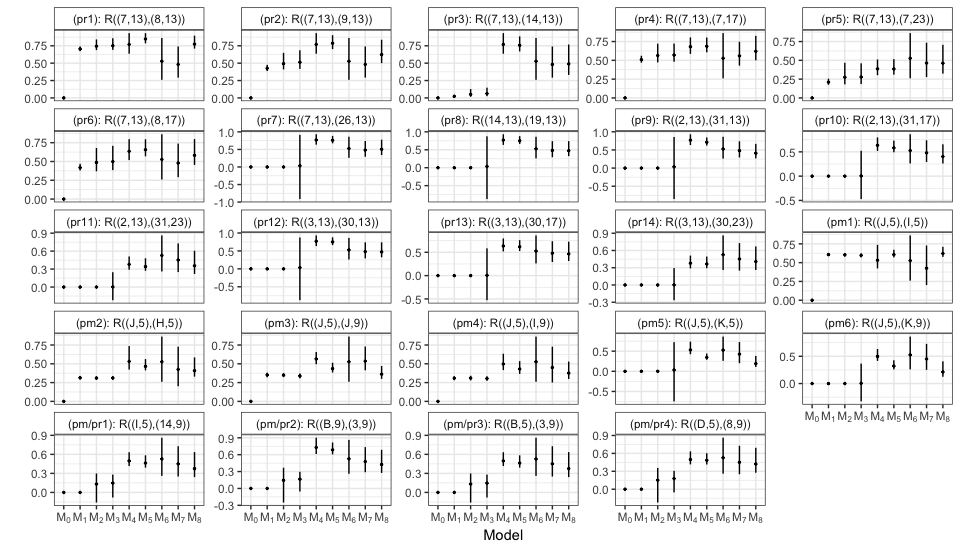
Figure B.11: Comparisons of the estimates of ${\bf R}$ from different models based on a specific set of elements. The panel titles include the panel name along with the tooth-time pair. The point estimate for each model is denoted by the dot, while the line shows the 95% confidence interval.

A comparison of the estimated correlation coefficients from ${\bf R}$ for the set of correlations from Table B.5 is presented in Figure B.11. Due to the independence misspecification, all the correlation elements in ${\mathcal{M}_{0}}$ are at zero. Models ${\mathcal{M}_{1}}$ and ${\mathcal{M}_{2}}$ have no connections between vertically-adjacent tooth-time pairs (panels: pr7-14), and the estimates and intervals are estimated to be zero. Model ${\mathcal{M}_{1}}$ additionally fails to estimate correlations between primary-permanent teeth in panels pm/pr1-4. We observe very wide credible intervals for ${\mathcal{M}_{3}}$ for some of correlation coefficients corresponding to vertically-adjacent tooth pairs. Overall, model ${\mathcal{M}_{6}}$, that assumes equicorrelation structure, seems to have the widest confidence intervals (except for the above ${\mathcal{M}_{3}}$ vertical adjacency issues). This seems reasonable as ${\boldsymbol{\theta}}_{D}$ consists of only one parameter specifying the complete correlation matrix ${\bf R}$, and, therefore, will have lower precision in estimation.

Tooth-location pair	Mean	95% CI	Interpretations
((7,13),(8,13))	0.774	(0.710, 0.896)	Same time, horizontally adjacent teeth
((7,13),(9,13))	0.623	(0.500, 0.837)	Same time, horizontally non-adjacent teeth
((7,13),(14,13))	0.489	(0.331, 0.767)	Same time, horizontally even farther teeth
((7,13),(7,17))	0.620	(0.500, 0.826)	Adjacent time, same tooth
((7,13),(7,23))	0.461	(0.323, 0.706)	Non-adjacent time, same tooth
((7,13),(8,17))	0.582	(0.454, 0.798)	Adjacent time, horizontally adjacent teeth
((7,13),(26,13))	0.505	(0.340, 0.779)	Adjacent time, vertically adjacent incisor teeth
((14,13),(19,13))	0.473	(0.323, 0.743)	Same time, vertically adjacent molar teeth
((2,13),(31,13))	0.409	(0.266, 0.669)	Same time, vertically adjacent molar teeth
((2,13),(31,17))	0.403	(0.260, 0.655)	Adjacent time, vertically adjacent molar teeth
((2,13),(31,23))	0.356	(0.218, 0.609)	Non-adjacent time, vertically adjacent molar teeth
((3,13),(30,13))	0.473	(0.323, 0.743)	Same time, vertically adjacent molar teeth
((3,13),(30,17))	0.465	(0.313, 0.729)	Adjacent time, vertically adjacent molar teeth
((3,13),(30,23))	0.407	(0.259, 0.670)	Non-adjacent time, vertically adjacent molar teeth
((J,5),(I,5))	0.622	(0.577, 0.711)	Same time, horizontally adjacent primary teeth
((J,5),(‘H,5))	0.408	(0.327, 0.585)	Same time, horizontally non-adjacent primary teeth
((J,5),(J,9))	0.362	(0.300, 0.471)	Adjacent time, same primary tooth
((J,5),(I,9))	0.375	(0.297, 0.530)	Adjacent time, adjacent primary teeth
((J,5),(K,5))	0.191	(0.108, 0.383)	Same time, vertically adjacent primary teeth
((J,5),(K,9))	0.212	(0.125, 0.410)	Adjacent time, vertically adjacent primary teeth
((I,5),(14,9))	0.376	(0.241, 0.636)	Adjacent time, primary/permanent molar teeth
((B,9),(3,9))	0.426	(0.276, 0.687)	Same time, primary/permanent molar teeth
((B,5),(3,9))	0.376	(0.241, 0.636)	Adjacent time, primary/permanent molar teeth
((D,5),(8,9))	0.421	(0.276, 0.694)	Adjacent time, primary/permanent incisor teeth

Table B.5: Approximate posterior estimates of specific representative elements from ${\bf R}({\boldsymbol{\theta}}_{D})$ for model ${\mathcal{M}_{8}}$. Tooth labels are found in Figure B.3.

B.4 Assessing Marginal Model Specification

We now describe two alternative marginal model specifications and consider similar validation strategies. The Poisson-hurdle model is often a standard choice for modeling count data when one does not expect the non-zero counts to be over-dispersed. The CDF for the marginal distribution of $Y_{ij}$ following Poisson hurdle model is given as,

$$\begin{array}[]{rcl}F_{ij}(y)=P(Y_{ij}\leq y)&=&\frac{1}{1+\exp({\boldsymbol{x}}_{ij}^{\prime}{\boldsymbol{\alpha}})}+\\ &&\left\{\frac{\exp(\boldsymbol{x}_{ij}^{\prime}{\boldsymbol{\alpha}})}{1+\exp(\boldsymbol{x}_{ij}^{\prime}{\boldsymbol{\alpha}})}\sum_{u=1}^{y}\mathrm{Pois}\left(u-1\mid\mu=\exp(\boldsymbol{x}_{ij}^{\prime}{\boldsymbol{\beta}})\right)\right\}\mathbb{I}(y>0),\end{array}$$ (B.2)

The marginal parameters will consist of ${\boldsymbol{\alpha}}$ and ${\boldsymbol{\beta}}$. We consider same Gaussian copula based dependence structure with the latent Gaussian vectors following the SAR model specifications described in Table 1. We first obtain the initial estimate for ${\boldsymbol{\theta}}$ under independence misspecification following an approach similar to the one described in Section A.1, but derived for Poisson hurdle model. An ABC-MCMC algorithm, modified accordingly, is then employed starting with the initial estimate of ${\boldsymbol{\theta}}$ and a set of posterior samples are obtained, which are then regression-adjusted to yield the final set of samples.

Another alternative choice for the marginal model is to simply consider the Negative Binomial model without any modeling of the zero inflation. That is, unlike our hurdle models, the excess zeros are not directly accounted for by the model and must be explained as part of the NB distribution. The dependence model specification remains the same with the corresponding NB CDF. All other computational details are as before.

For both of these models, we choose similar approach to parameter estimation. We obtain the initial estimates for the marginal parameters and their covariance by employing a Gibbs sampler under independence misspecification, and the initial estimates for the dependence parameters are obtained using an empirical approach as described in Section A.1. The summary statistics for the models come from the MLEs of their respective independence models as proposed in Section 4.2, and the kernel scaling matrix is also obtained similarly. For each model, we run three ABC-MCMC chains of length 185,000 each, and burnin the first 5000 samples. The remaining samples are regression-adjusted based on unique samples and are thinned to yield 9000 adjusted samples to be used for inference. All models are fit using the SAR structure ${\mathcal{M}_{8}}$.

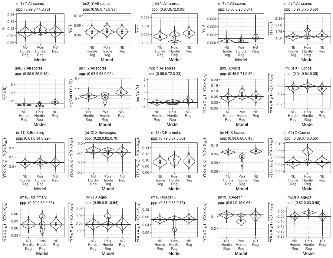
Figure B.12: Comparisons of the posterior predictive plots for marginal parameters from models with different marginal model specifications. The title of each plot shows the corresponding $ppp$ values ($ppp=0.00$ indicates $ppp<0.01$). $X_{1/3}$ and $X_{2/3}$ represent the first and second tertiles of predictor $X$, respectively.

.

Figure B.12 compares the posterior predictive distributions for the NB-Hurdle model against the two alternative choices to assess their marginal model fit using the same set of summary statistics as in Figure B.7. We observe that the NB model, which has to explain zero-inflation and over-dispersion with the same parameters overestimates the proportion of larger counts (panel: m3). The variance is also overestimated (panels: m7-m8). The Poisson-hurdle model shows quite competitve performance compared to NB-hurdle model. It is worth noting, however, that the effects of incisor teeth (panel: m14) and age 17 (panel: m19) are underestimated by the Poisson-hurdle model, while the age 23 effect (panel: 20) is overestimated. Overall NB-hurdle model turns out to be the best among all the marginal model choices.

Appendix C Further Details on Simulation Analysis

Here we present further details and analyses regarding our simulation study. First, we describe the true parameter values we chose to generate the simulated data. A brief account on the computation of the overall empirical coverage score is also included, followed by a discussion of the rank aggregation approach. In Section C.2, we investigate estimation of the parameters individually for different ABC-MCMC sampling strategies, including the classical rejection and importance sampling. The following subsection provides an alternative regression adjustment method and compares it against our proposed approach. Sensitivity of the model fit to the dependence structure specification is studied in Section C.4, where we evaluate estimation of the correct model against other models with misspecified dependence structures.

C.1 Additional Notes on Simulation Setup

We present the true data-generating parameter values used for the simulation setup in Table C.6. To replicate the relevant features of the IFS data in simulation setup, the true values of ${\boldsymbol{\theta}}_{M}$ and ${\boldsymbol{\theta}}_{D}$ are chosen to be close to the their respective point estimates obtained from fitting the IFS data with model ${\mathcal{M}_{4}}$.

Marginal Model Predictor (${\boldsymbol{\theta}}_{M}$)		Presence(${\boldsymbol{\alpha}}$)	Severity(${\boldsymbol{\beta}}$)
Intercept		-3.059	-0.831
Dental Appointments		-0.241	-0.196
Total fluoride ingested (mgF)		-0.003	-0.084
Frequency of brushing		-0.145	-0.040
Amount of sugar beverage (oz)		0.232	0.200
Tooth Type
Molar		Ref	–
Pre-Molar		-0.905	0.134
Incisor		-0.509	-0.150
Canine		-0.502	-0.245
Primary		-0.070	0.273
Observation Time
Age 5		-0.119	-0.114
Age 9		Ref	–
Age 13		-0.035	-0.206
Age 17		0.403	-0.001
Age 23		0.150	0.073
NB size $\phi$			0.865
SAR Model Parameters (${\boldsymbol{\theta}}_{D})$		Values
$\rho_{t}$		0.12
$\rho_{ct}$		0.012

Table C.6: True values for ${\boldsymbol{\theta}}_{M}$ and ${\boldsymbol{\theta}}_{D}$ for the simulation data generation.

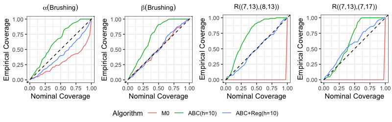
Figure C.13: Comparisons of the empirical coverage rates across different sampling strategies.

Before looking into the parameter estimation performance across different sampling strategies in the next section, we provide further clarity on the computation of the overall empirical coverage score (OECS). To that end, we consider two components from ${\boldsymbol{\theta}}_{M}$ and two from ${\boldsymbol{\theta}}_{\bf R}$ and show their empirical coverage curves for different model-fitting algorithms in Figure C.13. For simplicity, we only show the results for the best bandwidth, $h=10$. Observe that the coefficient for brushing frequency in the presence model is under-covered by ${\mathcal{M}_{0}}$, as its empirical coverage curve falls below the diagonal reference line. In contrast, ABC-MCMC over-covers the parameter, as its empirical coverage is consistently above the nominal rate. The regression adjustment, however, improves the coverage, with the true value of the parameter being covered at nearly the nominal coverage level across all levels $\zeta$ from 0 to 1. The OEC score, defined as the area under the empirical coverage curve, summarizes these observations and gives the best score (closest to 0.5) to the regression-adjusted ABC samples. In the case of the effect of brushing frequency in the severity model, the empirical coverage rates for both ${\mathcal{M}_{0}}$ and the regression-adjusted sample match the target coverage well. However, the unadjusted ABC samples over-cover the true coefficient. Regarding the correlation coefficients, ${\mathcal{M}_{0}}$ assumes all the correlations to be zero, and coverage rates are not estimated. For the purpose of comparison, we have shown the corresponding OEC scores indicating zero coverage. While ABC-MCMC samples perform better by learning the correlation structure from the data, they are plagued by some over-coverage which gets corrected by regression adjustment.

We now briefly provide some background on the rank aggregation strategy used to provide an overall ordering of the samplers. Let $\mathfrak{R}_{j}$ represent the ranked list of the samplers (the first sampler in $\mathfrak{R}_{j}$ being the “best”) for some collection $j=1,\ldots,J$ of ranked lists. For instance, in Table 3, the first collection considered is the (absolute) bias for the $j=27$ marginal parameters in ${\boldsymbol{\theta}}_{M}.$ While these individual lists/rankings are informative about a single parameter, “aggregating” them into a single consensus ranked list $\mathfrak{R}$ provides insight into the samplers’ performances overall; in this case, we use an aggregrated list to rank the methods in terms of the bias of the full set of ${\boldsymbol{\theta}}_{M}$ point estimators. To achieve this, we aggregate all $\mathfrak{R}_{j}$, using a Cross-Entropy Monte Carlo stochastic search proposed by Pihur et al., (2007). The idea is to find an optimal list $\mathfrak{R}$ that is closest to all the $\mathfrak{R}_{j}$, by minimizing the objective function $O(\mathfrak{R})=\sum_{j=1}^{J}d(\mathfrak{R},\mathfrak{R}_{j})$, where the sum is over the collection of lists considered. Here, $d(\cdot,\cdot)$ is chosen to be the Spearman footrule distance given by $d(\mathfrak{R},\mathfrak{R}_{j})=\sum_{t}|\mathfrak{r}(t)-\mathfrak{r}_{j}(t)|$, where $t$ represents the sampling method and $\mathfrak{r}(t)$ and $\mathfrak{r}_{j}(t)$ denote the ranks of method $t$ in $\mathfrak{R}$ and $\mathfrak{R}_{j}$, respectively. That is, the aggregated list $\mathfrak{R}$ minimizes the absolute differences of the rank of method $t$ in the consensus list $\mathfrak{R}$ and in the list $\mathfrak{R}_{j}$ across all methods $t$ and all lists $j$. Figure C.14(a) illustrates the rank aggregation visually for the bias of the marginal parameters. The raw ranks of the samplers are clearly highly variable across parameters, without any apparent overall ordering, since most methods had bias of approximately zero for all parameters. This lack of distinction among the performance of the samplers was also noted previously in Figure 2(m1) and in the corresponding discussion. The aggregated rank, marked with the solid black line, deviates from the dotted average rank line, suggesting that the average ranks do not differ much among the first 9 methods and that the average performance of these methods is similar among this set of lists.

Figure C.14: Raw, Aggregated and Average ranks of the samplers based on three different sets of ranking criteria described in the panel titles.

In contrast, there is more consistency in the individual rankings in Figure C.14(b), where we show sampler ranks for how well they cover the dependence model parameters. In this setting, the average rank is approximately the same as the aggregrate rank. Here, we have aggregated the collection $\mathfrak{R}_{1},\ldots,\mathfrak{R}_{J}$ representing the ranked list of OECS (absolute difference between OECS and $1/2$) for each of the $J=24$ correlation parameters in ${\boldsymbol{\theta}}_{\bf R}$. The corresponding boxplots in Figure 3(r3) have less overlap between methods, leading to a more clear ordering. Hence, the average ranks match more closely with the aggregated ranks. Similarly, Figure C.14(c) shows the raw, average and aggregated ranks based on RMSE for the correlation parameters. As with Figure 3(b), we have similar ordering across all constituent lists, the average rank, and the aggregated rank.

In Table 3 of the main manuscript, we have reported various aggregrated ranks by choosing different collections of $\mathfrak{R}_{1},\ldots,\mathfrak{R}_{J}$. The rankings are determined by ranking the performance of each parameter under each estimation criterion: the absolute bias for each parameter, RMSE for each parameter and the absolute difference between OECS and 0.5 for each parameter. The sets of rankings for each criterion are considered using only those parameters in the marginal model ${\boldsymbol{\theta}}_{M}$, using only the subset of correlation parameters ${\boldsymbol{\theta}}_{\bf R}$, and combining these two collections of rankings. In addition to obtaining a ranking under each criterion separately, we obtain an overall ranking by combining the per-parameter lists across the bias, RMSE and OECS criteria for ${\boldsymbol{\theta}}_{M}$, for ${\boldsymbol{\theta}}_{\bf R}$, and using the combined set of parameters. All these ranks are presented in Table 3.

C.2 Further Simulation Analysis

Here we compare the point estimates of the marginal and correlation parameters for the different sampling strategies. In Figures 2 and 3, we included violin plots showing the estimation accuracy summarized across the set of parameters in ${\boldsymbol{\theta}}_{M}$ and ${\boldsymbol{\theta}}_{\bf R}$, respectively. Here, we report the accuracy for each parameter individually in Tables C.7 and C.8. For brevity, we exclude results for all bandwidths except the optimal $h=10$, and we exclude the non-regression-adjusted rejection and importance sampling methods.

As discussed already in Section 6, we observe that estimation under the (unadjusted) ABC-MCMC sampler is not as good as ${\mathcal{M}_{0}}$, with the coverage for the severity model parameters ${\boldsymbol{\beta}}$ being particularly worse compared to ${\mathcal{M}_{0}}$. However, regression adjustment provides much better results across all the metrics. Overall, across all the sampling strategies, estimation of ${\boldsymbol{\beta}}$ is less accurate compared to ${\boldsymbol{\alpha}}$ of the presence model, which is reasonable considering there is less information available for model fit due to zero inflation. The Negative Binomial size parameter has the largest RMSE across the parameters. The ABC rejection sampler with regression adjustment also performs fairly well overall for the marginal parameters.

While investigating Table C.8 with the estimation performance for the selected elements of ${\bf R}$, we also consider estimation accuracy for the two individual SAR parameters. We observe that ABC-MCMC samples typically overcover both the SAR model parameters ${\boldsymbol{\theta}}_{D}$, which is corrected in regression adjustment, achieving the target coverage and increased accuracy in terms of bias and RMSE. The estimation of the individual ${\bf R}$ correlations is also improved from ABC-MCMC by the regression adjustment, while unadjusted samples have worse bias, worse RMSE and wider credible intervals providing overcoverage. The ABC rejection sampler does not work very well for ${\boldsymbol{\theta}}_{D}$ even after regression adjustment, with the estimation of $\rho_{ct}$ being particularly worse. This may be expected as the rejection sampler draws parameters from a non-informative prior with the true value of $\rho_{ct}$ lying near the boundary, resulting in a small number of accepted samples to work with.

	${\mathcal{M}_{0}}$			ABC-MCMC			ABC-MCMC + Regression			ABC-Rej + Regression			ABC-Imp + Regression
Parameters	Bias	RMSE	${\mathrm{OECS}}$	Bias	RMSE	${\mathrm{OECS}}$	Bias	RMSE	${\mathrm{OECS}}$	Bias	RMSE	${\mathrm{OECS}}$	Bias	RMSE	${\mathrm{OECS}}$
${\boldsymbol{\theta}}_{M}$
$\alpha$(Intercept)	-0.006	0.037	0.329	0.006	0.079	0.677	-0.002	0.046	0.467	-0.007	0.043	0.392	-0.006	0.002	0.332
$\alpha$(Visits)	0.000	0.038	0.284	0.011	0.081	0.628	0.006	0.047	0.416	-0.002	0.037	0.240	0.000	0.002	0.339
$\alpha$(Fluoride)	0.002	0.031	0.282	0.009	0.059	0.661	0.005	0.038	0.434	0.002	0.031	0.250	0.002	0.001	0.343
$\alpha$(Brushing)	0.003	0.036	0.273	0.009	0.071	0.627	0.006	0.043	0.390	0.003	0.035	0.225	0.004	0.002	0.293
$\alpha$(Beverages)	0.001	0.028	0.321	0.003	0.064	0.675	-0.001	0.036	0.468	0.001	0.029	0.312	0.003	0.001	0.346
$\alpha$(Pre-molar)	-0.004	0.033	0.462	0.013	0.078	0.729	-0.003	0.033	0.465	-0.004	0.032	0.435	-0.003	0.001	0.346
$\alpha$(Incisor)	0.002	0.027	0.527	0.016	0.067	0.733	0.004	0.026	0.529	0.001	0.027	0.522	0.000	0.001	0.351
$\alpha$(Canine)	-0.002	0.026	0.438	0.012	0.062	0.717	0.000	0.026	0.442	-0.003	0.028	0.437	-0.003	0.001	0.300
$\alpha$(Primary)	0.000	0.048	0.465	0.006	0.095	0.763	-0.002	0.046	0.442	-0.001	0.049	0.437	0.002	0.002	0.381
$\alpha$(Age5)	0.000	0.046	0.372	0.016	0.092	0.650	0.004	0.050	0.415	-0.002	0.047	0.377	0.000	0.003	0.325
$\alpha$(Age13)	0.001	0.039	0.518	0.003	0.082	0.787	0.000	0.041	0.542	0.000	0.038	0.464	0.002	0.002	0.411
$\alpha$(Age17)	0.005	0.039	0.400	-0.012	0.085	0.732	0.002	0.041	0.463	0.005	0.038	0.361	0.005	0.002	0.400
$\alpha$(Age23)	0.001	0.040	0.412	-0.015	0.084	0.674	-0.001	0.045	0.463	0.001	0.039	0.379	0.000	0.002	0.364
$\beta$(Intercept)	0.049	0.069	0.268	0.027	0.124	0.719	0.012	0.056	0.470	0.020	0.107	0.634	0.008	0.003	0.341
$\beta$(Visits)	0.019	0.047	0.411	0.079	0.121	0.367	0.016	0.049	0.451	0.004	0.051	0.506	0.007	0.002	0.368
$\beta$(Fluoride)	0.010	0.038	0.396	0.041	0.079	0.474	0.011	0.041	0.411	0.002	0.043	0.443	0.002	0.002	0.322
$\beta$(Brushing)	0.007	0.039	0.483	0.017	0.070	0.695	0.003	0.041	0.491	0.002	0.045	0.463	0.004	0.002	0.371
$\beta$(Beverages)	-0.015	0.033	0.457	-0.054	0.092	0.447	-0.008	0.035	0.516	-0.004	0.041	0.557	-0.001	0.001	0.379
$\beta$(Pre-molar)	-0.011	0.052	0.486	-0.075	0.115	0.350	-0.012	0.051	0.461	0.001	0.067	0.534	-0.004	0.003	0.350
$\beta$(Incisor)	0.012	0.048	0.496	0.074	0.117	0.375	0.006	0.048	0.472	0.002	0.068	0.541	-0.003	0.003	0.377
$\beta$(Canine)	0.044	0.062	0.295	0.106	0.149	0.301	0.013	0.054	0.424	0.008	0.071	0.503	0.008	0.003	0.337
$\beta$(Primary)	-0.025	0.080	0.443	-0.173	0.211	0.159	-0.033	0.078	0.405	-0.016	0.121	0.576	-0.010	0.006	0.361
$\beta$(Age5)	0.023	0.064	0.439	0.082	0.121	0.306	0.032	0.064	0.412	0.009	0.098	0.610	0.010	0.004	0.378
$\beta$(Age13)	0.039	0.079	0.414	0.122	0.168	0.268	0.003	0.071	0.461	-0.005	0.107	0.519	0.005	0.007	0.364
$\beta$(Age17)	-0.007	0.058	0.487	-0.006	0.082	0.826	-0.013	0.056	0.457	-0.013	0.084	0.529	-0.006	0.004	0.338
$\beta$(Age23)	-0.010	0.059	0.449	-0.046	0.096	0.490	-0.013	0.057	0.449	-0.009	0.085	0.499	-0.007	0.005	0.357
$\log\phi$	-0.013	0.092	0.536	-0.004	0.225	0.784	-0.011	0.091	0.517	0.032	0.206	0.640	-0.015	0.008	0.420

Table C.7: Average bias, RMSE and ${\mathrm{OECS}}$ for ${\boldsymbol{\theta}}_{M}$ from different sampling strategies. The bandwidth for ABC-MCMC is chosen to be 10.

	ABC-MCMC			ABC-MCMC + Regression			ABC-Rej + Regression			ABC-Imp + Regression
Parameters	Bias	RMSE	${\mathrm{OECS}}$	Bias	RMSE	${\mathrm{OECS}}$	Bias	RMSE	${\mathrm{OECS}}$	Bias	RMSE	${\mathrm{OECS}}$
${\boldsymbol{\theta}}_{D}$ elements
$\rho_{t}$	-0.005	0.028	0.716	-0.002	0.012	0.463	-0.081	0.125	0.229	-0.001	0.000	0.349
$\rho_{ct}$	-0.001	0.002	0.684	0.000	0.001	0.475	-0.346	0.412	0.000	0.000	0.000	0.552
${\boldsymbol{\theta}}_{R}$ elements
((7,13),(8,13))	-0.022	0.082	0.620	0.004	0.031	0.557	-0.197	0.197	0.000	0.008	0.001	0.421
((7,13),(9,13))	-0.022	0.082	0.620	0.004	0.031	0.557	-0.197	0.197	0.000	0.008	0.001	0.421
((7,13),(14,13))	-0.022	0.082	0.620	0.004	0.031	0.557	-0.197	0.197	0.000	0.008	0.001	0.421
((7,13),(7,17))	-0.022	0.079	0.670	0.000	0.033	0.488	-0.156	0.286	0.474	0.003	0.001	0.386
((7,13),(7,23))	-0.008	0.042	0.649	0.004	0.019	0.509	0.185	0.291	0.401	0.006	0.001	0.406
((7,13),(8,17))	-0.018	0.066	0.582	0.003	0.028	0.561	-0.119	0.120	0.000	0.005	0.001	0.419
((7,13),(26,13))	-0.022	0.082	0.620	0.004	0.031	0.557	-0.197	0.197	0.000	0.008	0.001	0.421
((14,13),(19,13))	-0.022	0.082	0.620	0.004	0.031	0.557	-0.197	0.197	0.000	0.008	0.001	0.421
((2,13),(31,13))	-0.022	0.082	0.620	0.004	0.031	0.557	-0.197	0.197	0.000	0.008	0.001	0.421
((2,13),(31,17))	-0.018	0.066	0.582	0.003	0.028	0.561	-0.119	0.120	0.000	0.005	0.001	0.419
((2,13),(31,23))	-0.008	0.036	0.574	0.003	0.017	0.568	-0.055	0.056	0.000	0.004	0.000	0.419
((3,13),(30,13))	-0.022	0.082	0.620	0.004	0.031	0.557	-0.197	0.197	0.000	0.008	0.001	0.421
((3,13),(30,17))	-0.018	0.066	0.582	0.003	0.028	0.561	-0.119	0.120	0.000	0.005	0.001	0.419
((3,13),(30,23))	-0.008	0.036	0.574	0.003	0.017	0.568	-0.055	0.056	0.000	0.004	0.000	0.419
((J,5),(I,5))	-0.015	0.053	0.654	0.000	0.017	0.543	-0.151	0.152	0.000	0.002	0.000	0.404
((J,5),(H,5))	-0.015	0.053	0.654	0.000	0.017	0.543	-0.151	0.152	0.000	0.002	0.000	0.404
((J,5),(J,9))	-0.020	0.069	0.684	-0.003	0.027	0.475	-0.152	0.270	0.433	0.000	0.001	0.363
((J,5),(I,9))	-0.015	0.050	0.581	0.000	0.019	0.550	-0.100	0.101	0.000	0.001	0.000	0.398
((J,5),(K,5))	-0.015	0.053	0.654	0.000	0.017	0.543	-0.151	0.152	0.000	0.002	0.000	0.404
((J,5),(K,9))	-0.015	0.050	0.581	0.000	0.019	0.550	-0.100	0.101	0.000	0.001	0.000	0.398
((I,5),(14,9))	-0.015	0.050	0.581	0.000	0.019	0.550	-0.100	0.101	0.000	0.001	0.000	0.398
((B,9),(3,9))	-0.022	0.077	0.622	0.002	0.027	0.551	-0.191	0.191	0.000	0.005	0.001	0.416
((B,5),(3,9))	-0.015	0.050	0.581	0.000	0.019	0.550	-0.100	0.101	0.000	0.001	0.000	0.398
((D,5),(8,9))	-0.015	0.050	0.581	0.000	0.019	0.550	-0.100	0.101	0.000	0.001	0.000	0.398

Table C.8: Average bias, RMSE and ${\mathrm{OECS}}$ for ${\boldsymbol{\theta}}_{D}$ and ${\boldsymbol{\theta}}_{R}$ from different sampling strategies. The bandwidth for ABC-MCMC is chosen to be 10.

To understand sensitivity of the ABC importance sampler to the bandwidth choice, we now compare its estimation performance without/with regression adjustment for different choices of $h$. Figure C.15 illustrates that, as the bandwidth increases, so does the bias, caused by the larger error in posterior approximation. Investigating the importance samples with smaller bandwidths $h=0.1$ and 1 for a few of the simulated datasets, we observed that the point estimate of ${\boldsymbol{\theta}}$ is dominated by fewer than 4 out of the 250,000 posterior samples, accounting for more than 95% of the total weight. Consequently, the credible intervals will be unreasonably narrow to be concentrated on these few points, leading to poor coverage, even if the point estimate is close to the target. Although larger bandwidths resulted in better overall coverage for the marginal parameters, this behavior was not consistent with the correlation parameters. To summarize, the importance sampler with small bandwidths is found to be completely impractical, as the posterior is based on a small collection of sample. While using a large bandwidth spreads the posterior weight across a larger collection of samples, the overall coverage is consistently below the normal rate after regression and the overall performance is inferior to the ABC-MCMC estimation approach, as discussed in Section 6.

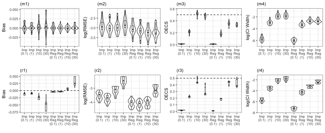
Figure C.15: Comparisons of performances of different ABC importance samplers across marginal parameters in panels (m1-m4) and across correlation parameters in panels (r1-r4).

C.3 Comparison of Regression Adjustment Strategies

We recall from Section 4.4 that the posterior samples $({\boldsymbol{\theta}}^{(g)},{\boldsymbol{s}}^{(g)})$ generated by the ABC-MCMC algorithm will have many repetitions. The design matrix ${\bf S}$ consisting of the ${\boldsymbol{s}}^{(g)}$ as rows is such that ${\bf S}^{\prime}{\bf S}$ is non-singular, which makes fitting the regression model problematic. We have avoided this issue by only using the unique samples from ABC-MCMC when fitting the regression model. We apply applying the regression adjustment to the (unweighted) sample of unique values and then reweighting them according to their frequency in the original ABC-MCMC chain. However, this strategy may not be optimal since we fit the heteroskedastic, locally linear regression model without using the weights from MCMC sampling (the abc function in the R library does not accomodate weighted samples).

We describe an alternative strategy that introduces noise to the original MCMC samples (with repeated values) to produce a sample with non-singular ${\bf S}^{\prime}{\bf S}$, but such that it does not affect the relationship between ${\boldsymbol{\theta}}$ and ${\boldsymbol{s}}$. To that end, let $\sigma_{s_{k}}^{2}$ denote the variance of the $k$-th summary statistic obtained from the full set of posterior samples ${\boldsymbol{s}}^{(g)}$ including replications. The $(g,k)$-th element $\tilde{s}^{(g)}_{k}$ of the modified design matrix $\widetilde{{\bf S}}$ is obtained as $\tilde{s}^{(g)}_{k}=s^{(g)}_{k}+\varepsilon_{k}$, where $\varepsilon_{k}\sim\text{Unif}(-0.001\sigma_{s_{k}},0.001\sigma_{s_{k}})$. We perform regression adjustment with the modified design matrix $\widetilde{{\bf S}}$.

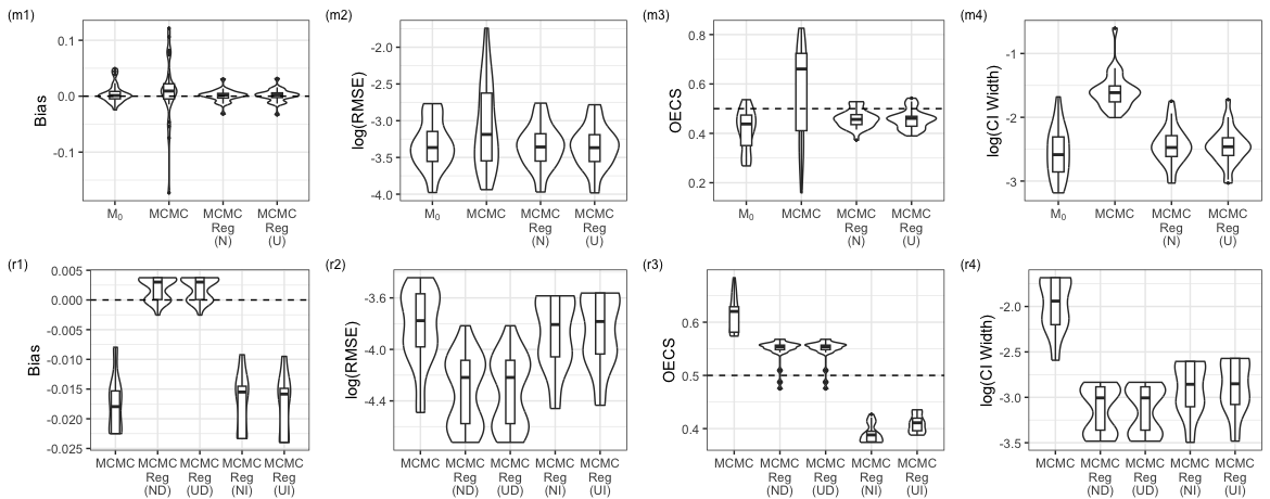
Figure C.16: Comparisons of estimation of ${\boldsymbol{\theta}}_{M}$ (in panels m1-m4) and ${\boldsymbol{\theta}}_{\bf R}$ (in panels r1-r4) across regression strategies. ‘N’ within braces indicates regression adjustment considering only unique samples, while ‘U’ indicates regression with addition of noise. Additionally for ${\boldsymbol{\theta}}_{\bf R}$, ‘D’ and ‘I’ stand for direct and indirect regression adjustment for the correlation coefficients, respectively.

The two regression adjustment strategies are now compared under our simulation setting. We use Reg(U) to represent our primary regression strategy of fitting the regression based on the unique samples, and Reg(N) represents regression adjustment with addition of noise. In the case of the marginal parameters ${\boldsymbol{\theta}}_{M}$, we compare estimation performance against the misspecified model ${\mathcal{M}_{0}}$, considered as the baseline, and with the data-generating model ${\mathcal{M}_{4}}$ using ABC-MCMC. The correlation coefficients ${\boldsymbol{\theta}}_{\bf R}$ can be adjusted in two ways, as discussed earlier in Section A.3: (D) direct adjustment of each correlation coefficient treating each component as a univariate estimand, or (I) indirect adjustment, achieved by adjusting ${\boldsymbol{\theta}}_{D}$ samples and using those to estimate the corresponding samples for the correlation coefficients. Note that the results reported previously in Section 6 are based on the (D) direct adjustment.

Figure C.16(m1-m4) shows that both the regression adjustment approaches yield very similar bias, RMSE, overall empirical coverage score (OECS), as well as credible interval width, for the marginal parameters. Using either is clearly superior in comparison to the unadjusted ABC samples and the independence model ${\mathcal{M}_{0}}$. Investigating the results for the correlation coefficients in Figure C.16 panels (r1-r4), we again observe minimal difference between the unique sample adjustment and its noisy version. However, bias and RMSE for the direct adjustment are meaningfully better than those for the indirect approach. The OEC scores are also noticably better under the direct adjustment, while the indirect approach shows under-coverage, with many OEC scores lying below 0.4. The credible intervals also seem to be narrower, showing superiority of the direct adjustment strategy. To understand this better, we recall from Appendix A.3 that indirect adjustment of ${\boldsymbol{\theta}}_{D}$ is challenging, as the support ${\boldsymbol{\Theta}}_{D}$ is not rectangular, requiring an additional post-regression adjustment step. Many of the regression-adjusted ${\boldsymbol{\theta}}_{D}$ samples fall outside the support, forcing shrinkage toward the corresponding unadjusted samples. The resulting bias for the indirectly adjusted samples resembles that for the ABC samples. This shrinkage also appears to cause undercoverage.

Ultimately, this investigation suggests that, at our optimal bandwidth $h=10$, our original regression strategy based on using only the unique samples from ABC-MCMC is basically equivalent to performing adjustment on the full sample after adding random noise. Investigating the differences in regression adjustment strategies using other bandwidths yields similar results under regression adjustment based on the unique sample or based on the noise-added samples. Further, we note that the indirect adjustment which was designed to respect the complex geometry of ${\boldsymbol{\Theta}}_{D}$ yields meaningfully worse estimation compared to applying direct univariate transformations for each parameter. Strategies for multivariate adjustments of non-rectangular parameter spaces requires further work in the future.

C.4 SAR Model Misspecification

To investigate the sensitivity of the model fit to the dependence model specification, we have fit a subset of alternative model choices to the simulation data sets, including ${\mathcal{M}_{1}}$, ${\mathcal{M}_{3}}$, ${\mathcal{M}_{4}}$ and ${\mathcal{M}_{5}}$ described in Table 1 (also Table B.4). Recall that the true data-generating model is ${\mathcal{M}_{4}}$, so analysis under these choices illustrates the impact of misspecifying the SAR form. Of note, the data-generating model ${\mathcal{M}_{4}}$ is nested within ${\mathcal{M}_{5}}$, so we anticipate ${\mathcal{M}_{5}}$ to give reasonable performance as well. We compute the same estimation performance metrics and compare against the true model ${\mathcal{M}_{4}}$ shown in Figure C.17.

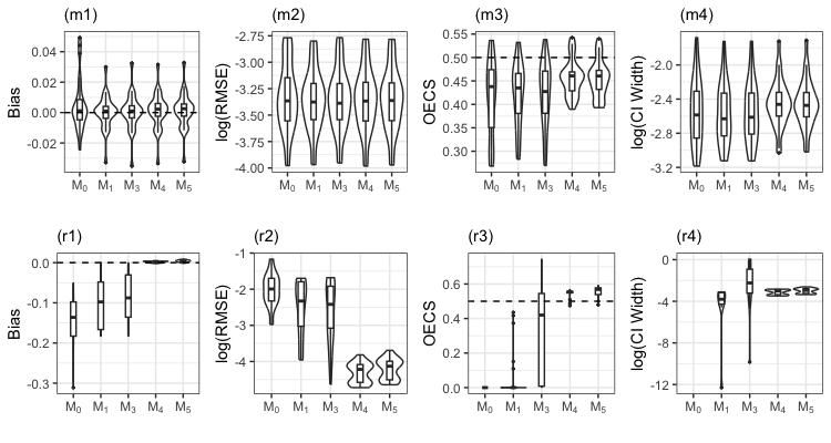
Figure C.17: Comparisons of ${\boldsymbol{\theta}}_{M}$ and ${\boldsymbol{\theta}}_{\bf R}$ across ${\mathcal{M}_{0}}$, ${\mathcal{M}_{1}}$, ${\mathcal{M}_{3}}$, ${\mathcal{M}_{4}}$ and ${\mathcal{M}_{5}}$. Recall ${\mathcal{M}_{4}}$ is the true data-generating model.

It is important to first note that all the models share the same marginal structure and, therefore, are expected to perform similarly in ${\boldsymbol{\theta}}_{M}$. We observe in Figure C.17 panels (m1-m4) that the biases across all the parameters are not very sensitive to the dependence model. The RMSEs are also similar across all the parameters. In terms of the overall empirical coverage score (OECS), the true model performs fairly well as expected, as does ${\mathcal{M}_{5}}$, with the scores across all the parameters close to the target 0.5. Models ${\mathcal{M}_{0}}$, ${\mathcal{M}_{1}}$ and ${\mathcal{M}_{3}}$ are farther away from the target, with somewhat higher variability among the scores. It is not surprising that ${\mathcal{M}_{5}}$ would have quite similar performance to ${\mathcal{M}_{4}}$ since this true data-generating model is contained within the parameter space of ${\mathcal{M}_{5}}$. Overall, estimation of the marginal parameters do not appear to be very sensitive to the dependence model.

Regarding the correlation parameters in Figure C.17 panels (r1-r4), the true model ${\mathcal{M}_{4}}$ estimates all the correlation parameters we considered with approximately zero bias, indicating that correlation estimation is accurate when the data are fit to the true model. It is not surprising that bias for ${\mathcal{M}_{5}}$ is close to zero, while we have meaningful bias under ${\mathcal{M}_{1}}$ and ${\mathcal{M}_{3}}$, as there is no parameter value within the parameter space of these models that can capture the ${\boldsymbol{\theta}}_{\bf R}$ from the data-generating model. Regardless, we do see closer estimation from these incorrect SAR models than under ${\mathcal{M}_{0}}$, which is “estimating” all correlations to be zero. We see similar trends in RMSE and OECS, with the true ${\mathcal{M}_{4}}$ having best performance and the other SAR models beating the independence model. We observe slightly higher RMSE and overall coverage rate for ${\mathcal{M}_{5}}$ due to the excess variability introduced by the extra parameter $\rho_{h}$. Note that the 95% equal-tailed credible interval for $\rho_{h}$ covered the true value ($\rho_{h}=0$) in 93 out of 100 simulated datas sets. Model ${\mathcal{M}_{3}}$ involves four parameters for the different adjacency relationships and is the most complex of the models. With these additional parameters, we see very large differences in the interval widths across the correlations considered. It is unclear whether this is associated with inconsistencies between fitting ${\mathcal{M}_{3}}$ when data are generated under ${\mathcal{M}_{4}}$ or whether this is associated with estimation of additional $\rho_{k}$s. Overall, the models that contain the data generation (${\mathcal{M}_{4}}$ and ${\mathcal{M}_{5}}$) accurately estimate the marginal models and the dependence, while all SAR models have acceptable estimation of the ${\boldsymbol{\theta}}_{M}$ parameters even under misspecification of the dependence.

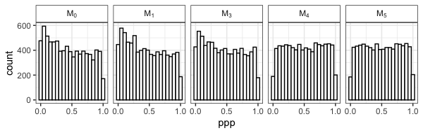
Figure C.18: Histogram of all available $ppp$-values across all model choices.

To conclude this section, we now briefly describe the process of using the $ppp$ values for model comparison across SAR choices as was utilized for model selection in the IFS case (see Appendix B.3). While we show these posterior predictive checks for only one of the simulated datasets, we note that the behavior is similar across the other simulated datasets used in the simulation. The histograms of $ppp$ values across the complete set of Spearman correlations are shown in Figure C.18. We see that ${\mathcal{M}_{0}}$ has the highest skewness toward zero, which is expected due to its independence misspecification. As model ${\mathcal{M}_{1}}$ assumes independence among vertically-adjacent tooth pairs or primary/permanent teeth, it also involves many exact zeros in the correlation matrix and is inadequate for modeling the dependence of model ${\mathcal{M}_{4}}$. This is apparent from the higher concentration of $ppp$ near zero. While ${\mathcal{M}_{3}}$ does not have exact zeros in its inverse, it is still sparse and a misspecified model here, as indicated by another peak near zero. In contrast, the true data-generating model ${\mathcal{M}_{4}}$ and the model encompassing the truth ${\mathcal{M}_{5}}$ have no evidence of inadequency, as the distribution of $ppp$ is not skewed toward zero. If performing model selection here, one would immediately limit attention to ${\mathcal{M}_{4}}$ and ${\mathcal{M}_{5}}$ as the two best performing models; as ${\mathcal{M}_{4}}$ is more parsimonious, it is likely to be the model that would be chosen. Thus, following the same strategy as was used in the IFS data analysis, we have determined the true data-generating model to be the best model and the model to use for inference in this simulated example.

References

- Andrieu and Thoms, (2008) Andrieu, C. and Thoms, J. (2008). A tutorial on adaptive MCMC. Statistics and Computing, 18(4):343–373.
- Badinger and Egger, (2011) Badinger, H. and Egger, P. (2011). Estimation of higher-order spatial autoregressive cross-section models with heteroscedastic disturbances. Papers in Regional Science, 90(1):213–235.
- Banerjee et al., (2004) Banerjee, S., Carlin, B., and Gelfand, A. (2004). Hierarchical Modeling and Analysis of Spatial Data, volume 101. Chapman & Hall/CRC Monographs on Statistical and Applied Probability.
- Beaumont, (2019) Beaumont, M. A. (2019). Approximate Bayesian computation. Annual Review of Statistics and Its Application, 6:379–403.
- Beaumont et al., (2002) Beaumont, M. A., Zhang, W., and Balding, D. J. (2002). Approximate Bayesian Computation in Population Genetics. Genetics, 162(4):2025–2035.
- Besag, (1974) Besag, J. (1974). Spatial Interaction and the Statistical Analysis of Lattice Systems. Journal of the Royal Statistical Society: Series B (Methodological), 36(2):192–225.
- Blum and François, (2010) Blum, M. G. B. and François, O. (2010). Non-linear regression models for Approximate Bayesian Computation. Statistics and Computing, 20(1):63–73.
- Bonassi and West, (2015) Bonassi, F. V. and West, M. (2015). Sequential Monte Carlo with Adaptive Weights for Approximate Bayesian Computation. Bayesian Analysis, 10(1):171–187.
- Broffitt et al., (2013) Broffitt, B., Levy, S. M., Warren, J., and Cavanaugh, J. E. (2013). Factors associated with surface-level caries incidence in children aged 9 to 13: The Iowa Fluoride Study. Journal of Public Health Dentistry, 73(4):304–310.
- Carvalho et al., (2010) Carvalho, C. M., Polson, N. G., and Scott, J. G. (2010). The horseshoe estimator for sparse signals. Biometrika, 97(2):465–480.
- Choo-Wosoba et al., (2018) Choo-Wosoba, H., Gaskins, J., Levy, S., and Datta, S. (2018). A Bayesian approach for analyzing zero-inflated clustered count data with dispersion. Statistics in Medicine, 37(5):801–812.
- Choo-Wosoba et al., (2016) Choo-Wosoba, H., Levy, S. M., and Datta, S. (2016). Marginal regression models for clustered count data based on zero-inflated Conway-Maxwell-Poisson distribution with applications. Biometrics, 72(2):606–618.
- Csilléry et al., (2012) Csilléry, K., François, O., and Blum, M. G. B. (2012). abc: an R package for approximate Bayesian computation (ABC). Methods in Ecology and Evolution, 3(3):475–479.
- Daniels and Hogan, (2008) Daniels, M. and Hogan, J. (2008). Missing Data in Longitudinal Studies: Strategies for Bayesian Modeling and Sensitivity Analysis. Chapman & Hall/CRC Monographs on Statistics & Applied Probability. Taylor & Francis.
- Debarsy and LeSage, (2022) Debarsy, N. and LeSage, J. P. (2022). Bayesian Model Averaging for Spatial Autoregressive Models Based on Convex Combinations of Different Types of Connectivity Matrices. Journal of Business & Economic Statistics, 40(2):547–558.
- Drovandi et al., (2011) Drovandi, C. C., Pettitt, A. N., and Faddy, M. J. (2011). Approximate Bayesian computation using indirect inference. Journal of the Royal Statistical Society. Series C: Applied Statistics, 60(3):317–337.
- Elhorst et al., (2012) Elhorst, J. P., Lacombe, D. J., and Piras, G. (2012). On model specification and parameter space definitions in higher order spatial econometric models. Regional Science and Urban Economics, 42(1-2):211–220.
- Fagundes et al., (2007) Fagundes, N. J. R., Ray, N., Beaumont, M., Neuenschwander, S., Salzano, F. M., Bonatto, S. L., and Excoffier, L. (2007). Statistical evaluation of alternative models of human evolution. Proceedings of the National Academy of Sciences, 104(45):17614–17619.
- Fan and Sisson, (2018) Fan, Y. and Sisson, S. A. (2018). ABC Samplers. In Handbook of Approximate Bayesian Computation, chapter 4, pages 87–123. Chapman and Hall/CRC.
- Fearnhead and Prangle, (2012) Fearnhead, P. and Prangle, D. (2012). Constructing summary statistics for approximate Bayesian computation: semi-automatic approximate Bayesian computation. J. R. Statist. Soc. B, 74:419–474.
- Gelman et al., (1996) Gelman, A., Meng, X.-L., and Stern, H. (1996). Posterior predictive assessment of model fitness via realized discrepancies. Statistica Sinica, 6(4):733–760.
- Gelman and Rubin, (1992) Gelman, A. and Rubin, D. B. (1992). Inference from Iterative Simulation Using Multiple Sequences. Statistical Science, 7(4):457–472.
- Griffin and Brown, (2010) Griffin, J. E. and Brown, P. J. (2010). Inference with normal-gamma prior distributions in regression problems. Bayesian Analysis, 5(1):171–188.
- Hjort et al., (2006) Hjort, N. L., Dahl, F. A., and Steinbakk, G. H. (2006). Post-Processing Posterior Predictive p Values. Journal of the American Statistical Association, 101(475):1157–1174.
- Ionides, (2008) Ionides, E. L. (2008). Truncated importance sampling. Journal of Computational and Graphical Statistics, 17(2):295–311.
- Jin et al., (2016) Jin, I. H., Yuan, Y., and Bandyopadhyay, D. (2016). A Bayesian hierarchical spatial model for dental caries assessment using non-Gaussian Markov random fields. The Annals of Applied Statistics, 10(2):884–905.
- Kang et al., (2021) Kang, T., Gaskins, J., , S., and Datta, S. (2021). A longitudinal Bayesian mixed effects model with hurdle Conway-Maxwell-Poisson distribution. Statistics in Medicine, 40(6):1336–1356.
- Kang et al., (2023) Kang, T., Gaskins, J., Levy, S., and Datta, S. (2023). Analyzing dental fluorosis data using a novel Bayesian model for clustered longitudinal ordinal outcomes with an inflated category. Statistics in Medicine, 42(6):745–760.
- Kolev and Paiva, (2009) Kolev, N. and Paiva, D. (2009). Copula-based regression models: A survey. Journal of Statistical Planning and Inference, 139(11):3847–3856.
- Levy et al., (2003) Levy, S. M., Warren, J. J., Broffitt, B., Hillis, S. L., and Kanellis, M. J. (2003). Fluoride, beverages and dental caries in the primary dentition. Caries Research, 37(3):157–165.
- Little and Rubin, (2019) Little, R. and Rubin, D. (2019). Statistical Analysis with Missing Data. Wiley Series in Probability and Statistics. Wiley, 3 edition.
- Marjoram et al., (2003) Marjoram, P., Molitor, J., Plagnol, V., and Tavaré, S. (2003). Markov chain Monte Carlo without likelihoods. Proceedings of the National Academy of Sciences of the United States of America, 100(26):15324–15328.
- Mitra et al., (2023) Mitra, R., McGough, S. F., Chakraborti, T., Holmes, C., Copping, R., Hagenbuch, N., Biedermann, S., Noonan, J., Lehmann, B., Shenvi, A., Doan, X. V., Leslie, D., Bianconi, G., Sanchez-Garcia, R., Davies, A., Mackintosh, M., Andrinopoulou, E.-R., Basiri, A., Harbron, C., and MacArthur, B. D. (2023). Learning from data with structured missingness. Nature Machine Intelligence, 5(1):13–23.
- Neelon, (2019) Neelon, B. (2019). Bayesian zero-inflated negative binomial regression based on Pólya-Gamma mixtures. Bayesian Analysis, 14(3):829–855.
- Neuhaus et al., (1991) Neuhaus, J. M., Kalbfleisch, J. D., and Hauck, W. W. (1991). A Comparison of Cluster-Specific and Population-Averaged Approaches for Analyzing Correlated Binary Data. International Statistical Review / Revue Internationale de Statistique, 59(1):25.
- Nunes and Balding, (2010) Nunes, M. A. and Balding, D. J. (2010). On optimal selection of summary statistics for approximate bayesian computation. Statistical Applications in Genetics and Molecular Biology, 9(1). doi: 10.2202/1544-6115.1576.
- Pace et al., (2000) Pace, R., Barry, R., Gilley, O. W., and Sirmans, C. (2000). A method for spatial–temporal forecasting with an application to real estate prices. International Journal of Forecasting, 16(2):229–246.
- Park and Casella, (2008) Park, T. and Casella, G. (2008). The Bayesian Lasso. Journal of the American Statistical Association, 103(482):681–686.
- Pihur et al., (2007) Pihur, V., Datta, S., and Datta, S. (2007). Weighted rank aggregation of cluster validation measures: A Monte Carlo cross-entropy approach. Bioinformatics, 23(13):1607–1615.
- Pihur et al., (2008) Pihur, V., Datta, S., and Datta, S. (2008). Finding common genes in multiple cancer types through meta–analysis of microarray experiments: A rank aggregation approach. Genomics, 92(6):400–403.
- Pillow and Scott, (2012) Pillow, J. W. and Scott, J. G. (2012). Fully Bayesian inference for neural models with negative-binomial spiking. Advances in Neural Information Processing Systems, 3:1898–1906.
- Pitt et al., (2006) Pitt, M., Chan, D., and Kohn, R. (2006). Efficient Bayesian inference for Gaussian copula regression models. Biometrika, 93(3):537–554.
- Polson et al., (2013) Polson, N. G., Scott, J. G., and Windle, J. (2013). Bayesian Inference for Logistic Models Using Pólya-Gamma Latent Variables. Journal of the American Statistical Association, 108(504):1339–1349.
- Pudlo et al., (2016) Pudlo, P., Marin, J.-M., Estoup, A., Cornuet, J.-M., Gautier, M., and Robert, C. P. (2016). Reliable ABC model choice via random forests. Bioinformatics, 32(6):859–866.
- Rubin, (1984) Rubin, D. B. (1984). Bayesianly Justifiable and Relevant Frequency Calculations for the Applied Statistician. The Annals of Statistics, 12(4):1151–1172.
- Sisson et al., (2018) Sisson, S. A., Fan, Y., and Beaumont, M. (2018). Handbook of Approximate Bayesian Computation. Chapman and Hall/CRC.
- Sisson et al., (2007) Sisson, S. A., Fan, Y., and Tanaka, M. M. (2007). Sequential Monte Carlo without likelihoods. Proceedings of the National Academy of Sciences, 104(6):1760–1765.
- Smith and Khaled, (2012) Smith, M. S. and Khaled, M. A. (2012). Estimation of copula models with discrete margins via Bayesian data augmentation. Journal of the American Statistical Association, 107(497):290–303.
- Spiegelhalter et al., (2002) Spiegelhalter, D. J., Best, N. G., Carlin, B. P., and Van Der Linde, A. (2002). Bayesian Measures of Model Complexity and Fit. Journal of the Royal Statistical Society Series B: Statistical Methodology, 64(4):583–639.
- Uddin and Gaskins, (2023) Uddin, M. N. and Gaskins, J. T. (2023). Shared Bayesian variable shrinkage in multinomial logistic regression. Computational Statistics & Data Analysis, 177:107568.
- Vehtari et al., (2022) Vehtari, A., Simpson, D., Gelman, A., Yao, Y., and Gabry, J. (2022). Pareto Smoothed Importance Sampling. arXiv:1507.02646 [stat].