Boundary conditions and violations of bulk-edge correspondence in a hydrodynamic model
Abstract
Bulk-edge correspondence is a wide-ranging principle that applies to topological matter, as well as a precise result established in a large and growing number of cases. According to the principle, the distinctive topological properties of matter, thought of as extending indefinitely in space, are equivalently reflected in the excitations running along its boundary, when one is present. Indices encode those properties, and their values, when differing, are witness to a violation of that correspondence. We address such violations, as they are encountered in a hydrodynamic context. The model concerns a shallow layer of fluid in a rotating frame and provides a local description of waves propagating either across the oceans or along a coastline; it becomes topological when suitably modified at short distances. The edge index is sensitive to boundary conditions, as exemplified in earlier work, hence exhibiting a violation. Here we present classification of all (local, self-adjoint) boundary conditions and a parameterization of their manifold. They come in four families, distinguished in part by the degree of their underlying differential operators. Essentially, that degree counts the degrees of freedom of the hydrodynamic field that are constrained at the boundary by way of their normal derivatives. Generally, both the correspondence and its violation are typical. Within families though, the maximally possible amount of violation is increasing with its degree. Several indices of interest are charted for all boundary conditions. A single spectral mechanism for the onset of violations is furthermore identified. The role of a symmetry is investigated.
1 Introduction
Topological considerations in physics have risen to a prominent role in the quantum domain, notably with the Quantum Hall Effect [1]. Later developments took place in the classical domain, and among them in hydrodynamics [2, 3, 4]. The present work lies in that same context.
A sweeping concept in the realm of topological matter is bulk-edge correspondence (BEC); in fact to the extent that it is often taken for granted. In essence, it states that such systems admit two topological indices, independently defined, but coinciding in value. The first one, known as the bulk index, is associated in physical terms to the infinitely extended and gapped system, and in more mathematical ones to some compact manifold, such as the Brillouin zone. The second index, i.e. the edge index, is by contrast associated to a system now having a spatial boundary. The index arises by way of a count of edge states, chiral or otherwise, found at energies previously lying in the gap. See the selected references [5, 6, 7], and [8] for a pedagogical review.
The correspondence was first established in the context of the Integer Quantum Hall Effect [9, 10, 11, 12, 13], and soon extended to a variety of other models, possibly having special symmetry properties [14, 15, 16, 17], yet dealing with independent particles. Different techniques were used and, among them, scattering theory related to Levinson’s theorem [18]. That approach [19] will play some role presently.
Models enjoying a continuous translational symmetry lack a compact momentum space, thus putting the bulk index in need of attention. Some extensions in this direction appeared in the literature and were obtained with a wide range of mathematical tools, ranging from bifurcation theory for PDEs [20] to homotopy of Fredholm operators [21] and more [22, 23]. Notice that BEC was shown to hold in various models with “soft” boundaries, namely thick interface regions between different insulators [24, 25].
In contrast to the aforementioned results, that aimed at extending the validity of BEC, the present work attempts to pinpoint its limits and violations. We shall do so in the context of a hydrodynamic model, known as the rotating shallow water model (SWM), thus extending the analysis of special cases [26, 2, 19] to the generality that is proper to the model.
The rotating shallow water model describes an incompressible fluid lying on a rotating, flat bottom. It is derived from Euler’s equations by linearizing and assuming small fluid height relative to the typical wavelength. It is used to describe certain oceanic and atmospheric layers on Earth [27], where the Coriolis force plays the same role as the magnetic field in the quantum Hall effect [28]. Remarkably, it explains the stability of the eastward-propagating Kelvin equatorial wave [29] by recognizing its topological nature.
The model is defined by a system of partial differential equations (PDEs) that are formally equivalent to a Schrödinger equation, whence a similar treatment as used for quantum mechanical systems becomes feasible. The corresponding Hamiltonian is formally that of a topological insulator of symmetry class D according to the periodic table of topological matter [30, 31]. In order to restore the desired compactness, as hinted at before, we shall consider a variant of the model, that is characterized by odd viscosity [32], and which provides a small-scale regularization. Indeed, the latter in turn allows for a compactification of the (otherwise unbounded) momentum space and for a proper topological definition of the bulk index.
If BEC were to hold in the form introduced above, this bulk invariant should predict the number of chiral modes appearing when a boundary, i.e. a coastline in the hydrodynamic setting, is introduced. This is however not always the case. As shown in [19], the number of edge modes depends on the boundary conditions imposed on the coastline, thus invalidating BEC, whose claim does not depend on details of the boundary.
Ref. [19] calls for systematic and extensive investigation on violations of bulk-edge correspondence. This work considers and answers the following questions:
-
Q1
What are the most general local self-adjoint boundary conditions for this model? And what can be said about BEC for them?
-
Q2
What is the most natural edge index, i.e. the best way to count edge states merging with the (bulk) continuum?
-
Q3
Are there other integers of interest?
-
Q4
What relations, like BEC or otherwise, exist between them? Do they hold unconditionally?
Before detailing the structure of this paper, we briefly review some recent literature. Like our work, Refs. [33, 34, 35] focus on bulk-edge correspondence in the shallow water model. Ref. [33] defines an edge index via spectral flow and “averaging” over a loop of boundary conditions. This index coincides with its bulk counterpart. Ref. [34] studies topological properties of the SWM on a spherical geometry. Ref. [35] forgoes odd-viscous regularization, and considers a Coriolis force that varies in space, producing an interface where it crosses zero. Violations of BEC are displayed for certain discontinuous profiles of the Coriolis force. Other recent works concern the 2D Dirac Hamiltonian, which is closely related to the SWM when viewing both as spin models. An ultraviolet-regularized Dirac is shown to host violations of BEC in [36]. In fact, boundary conditions are comprehensively classified, based on whether they do, or do not, lead to bulk-edge correspondence. Finally, [37] notices that BEC is restored for magnetic Dirac operators, at least with infinite-mass boundary conditions .
Broadly speaking, this paper consists of three parts. The first part, comprising Sects. 2 and 3, introduces the setup and main results, while glossing over a number of technical details. The second part, comprising Sects. 4, 5, expands on the details omitted in the first one, and culminates in the statement of broader, more precise results. The third part, comprising Sects. 6 and 7, contains proofs, preceded by a preliminary exposition of the techniques used.
More precisely, Sect. 2.1 introduces the infinitely extended (bulk) shallow water model, its Hamiltonian and properties of the latter. Among them: Spectrum, particle-hole symmetry (PHS), associated Bloch bundle. A bulk index is moreover defined through a compactification of momentum space. In Sect. 2.2, the edge model is introduced by restricting physical space to the upper half-plane. Local boundary conditions, and associated von Neumann unitaries, are defined and grouped into four qualitatively different families DD, ND, DN, NN. A special role is played by those that preserve PHS. In Sect. 2.3, we define our edge index as the number of proper () and improper () edge eigenvalues merging with the bulk band of interest. Further relevant integers are , the number of asymptotically flat edge eigenvalues, and the winding of the boundary condition. The indices collectively form an index vector .
In Sect. 3, results are reported in terms of the index vector . Its values are charted in the three families DD, ND, DN, and in the particle-hole symmetric subfamily of the fourth one, NN. Violations of bulk-edge correspondence are proven “typical”, and a single violation-inducing mechanism is identified.
Sect. 4.1 provides further details on the bulk Hamiltonian, focusing on its eigenstates and the compactification of momentum space that enables the definition of the bulk index. Sect. 4.2 reviews the scattering theory of shallow-water waves. The scattering amplitude is introduced, and its poles identify edge eigenvalues. In Sect. 4.3, we connect to the bulk and edge indices at once, making it the central tool for detecting bulk-edge correspondence or lack thereof. Sect. 4.4 contains further details on self-adjoint boundary conditions, and a parametrization of the aforementioned families and associated unitaries.
Sect. 5 deepens the results of Sect. 3 by directly relating parameters of the boundary conditions to values of , and extends those same results by treating the full family NN (rather than its particle-hole symmetric subfamily).
Sects. 6.1, 6.2, 6.3, 6.4 detail how the evaluation of the integer , , , is performed, respectively, given certain boundary conditions. Finally, Sect. 7 presents the full proofs of the results of Secs. 3, 5.
The appendices either contain additional results that are not essential to the main discussion, or proofs which were omitted in the interest of readability.
2 Setup
In this section, we will provide an overview of the model and introduce the notions needed in order to state the results in Sect. 3. We shall discuss the bulk picture, including its geometric objects, to be followed by the edge picture, including a first discussion of the possible boundary conditions, that will turn out to be of four main types.
2.1 Bulk model
The rotating and odd-viscous shallow water model is a 2D hydrodynamical model describing a thin layer of incompressible fluid that lies on a flat, rotating bottom extending over the whole plane. Its physical relevance, its derivation by linearization, as well as its applications will not be treated in this work. The interested reader is referred to [29, 26, 2, 19].
The model is governed by the following system of linear PDEs
| (2.1) |
where is the velocity field on the -plane, the height of the fluid w.r.t. to the undisturbed fluid level; while the parameters determine the Coriolis force and the (odd) viscosity force , respectively. We denote the Laplacian by and assume for simplicity, as will become clear later.
The system of equations (2.1) is formally equivalent to a Schrödinger equation , with wave function , () and Hamiltonian given as
| (2.2) |
Let us at first regard as a formal differential operator. Being translation invariant, its normal modes are of the form
| (2.3) |
with bulk solutions of the time-independent eigenvalue problem (see Sect. 4.1)
| (2.4) |
where . The differential operator is realized as a self-adjoint operator on the Hilbert space , with domain given in terms of Sobolev spaces as .
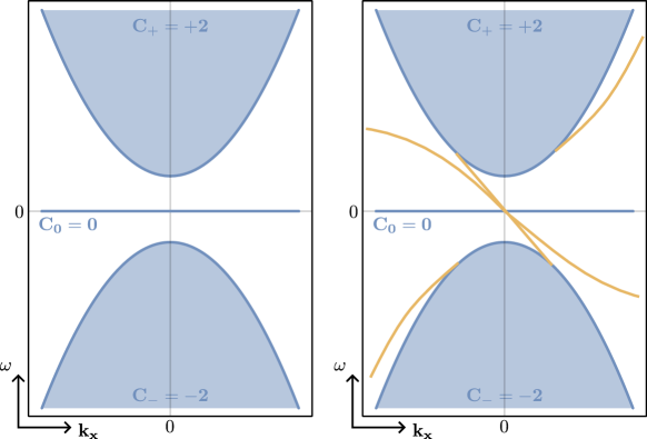
The spectrum of is purely essential [38] and consists of three bands, labeled . They arise from the discrete spectrum of , consisting of eigenvalues (cf. Fig. 1):
| (2.5) |
The bands are separated by gaps of size at . Let moreover
| (2.6) |
denote the lower rim of the upper band.
Momentum space is unbounded, reflecting that translations give rise to a continuous symmetry group. As we shall see in Sect. 4.1, the regularization provided by ensures the eigenspaces of converge as , thus allowing for a description based on the -point compactification of .
We shall call Bloch bundle the trivial vector bundle . It decomposes as
| (2.7) |
where
| (2.8) |
is the eigenbundle determined by the eigenprojections of the eigenvalues , i.e. , , cf. [19] for details. The Chern numbers , associated to the bands are proper topological invariants, in view of the compactness of . They amount to
| (2.9) |
as shown in [19], Prop. 2.1.
The Hamiltonian enjoys an antiunitary symmetry, formally akin to (even) particle-hole (pseudo-) symmetry (PHS) [39],
| (2.10) |
with denoting complex conjugation. Clearly, . The Hamiltonian enjoys no further symmetry among those contemplated in the AZK table [30, 31]. It thus sits in class .
In the following, we will only focus on the upper band, the middle one being trivial, and . We will refer to
| (2.11) |
as the bulk index. Its value, , will be compared to that of other indices, that arise by restriction to a half-plane.
2.2 Edge picture and boundary conditions
Let us now introduce the edge picture. Details that are not needed for the statement of the results will be returned upon in Sects. 4.2, 4.4.
A boundary is introduced by restricting the physical space to the upper half-plane
| (2.12) |
Since translation invariance is retained in the -direction only, normal modes of the formal differential operator (2.2) are of the form
| (2.13) |
where is in turn a normal mode of the formal differential operator
| (2.14) |
These modes are more general than the modes (2.3) in that they can be evanescent, i.e. decaying transversally.
The formal differential operator (2.14) is likewise promoted, as in the previous section, to a self-adjoint operator on the Hilbert space , by way of specifying suitable boundary conditions that define its domain .
Not all boundary conditions correspond to a self-adjoint realization of . Von Neumann’s theory of self-adjoint extensions builds on the deficiency spaces at of the (closed) operator realizing the differential operator with minimal domain. It then expresses the extensions in terms of unitary maps between the two spaces; cf. ([40], Thm. X.2).
We shall determine all self-adjoint boundary conditions that are
-
(i)
local,
-
(ii)
invariant under translation along the boundary, and
-
(iii)
involve derivatives of the wave function of order 1 at most.
Let us first focus on conditions (i, ii). As a result, the deficiency spaces are those of a minimal realization of , cf. (2.14). The defect indices of the latter are finite, and in fact . The extensions of the formal differential operator (2.14) are thus in some correspondence with unitary matrices of order 2, (cf. Sect. 4.4 and App. A). The same extensions can also be expressed in terms of two boundary conditions involving and at
| (2.15) |
whence is a matrix that, far from being arbitrary, satisfies conditions (to be discussed in Sect. 4.4) arising from the requirement of self-adjointness.
Any such determines , but not conversely. Rather, determines the orbit of under multiplication from the left by ,
| (2.16) |
This reflects the fact that the two boundary conditions are unaltered when replaced by linearly independent linear combinations.
By including requirement (iii) above, the boundary conditions are of the general form
| (2.17) |
with
| (2.18) |
Eq. (2.17) then implies that the dependence in (2.15) is affine. Alternatively, will turn out to be a fractional linear transformation with coefficients in . Moreover, a linear recombination of the rows of Eq. (2.17) amounts to , cf. (2.16), being a constant matrix.
Remark 2.1.
Both the context of Eq. (2.16), which is pointwise in , and that of (2.17), which is global, induce a notion of orbit, . They are the orbits under local vs global gauge transformations, i.e. vs , acting by left multiplication. The former orbits are of course larger, and decompose into the latter. We take the point of view that only ’s arising from (2.17) are to be considered, but any two of them shall be considered equivalent in the sense of (2.16). This reflects the fact that this notion characterizes a same half-plane Hamiltonian .
The complete, intrinsic characterization of the objects so obtained will be given in Sec. 4.4. The following operative definition will be useful. The cross-references to App. A fill the details that were left open up to now, but can be skipped still.
Definition 2.2 (Boundary condition and von Neumann unitary).
We partition the set of self-adjoint boundary condition into the following four families.
Definition 2.4 (Families of boundary conditions).
Clearly, the conditions are compatible with (2.16). The middle case will be subdivided into two (overlapping) families in Lm. 4.4. As will also be explained in Sect. 4.4, the two families are related by a substitution, by way of which results can be carried over between them. As they remain structurally unaffected, only the case ND will be pursued.
The labeling by symbols D and N comes about as follows. We distinguish between generalized Neumann (N, a.k.a. Robin or mixed) and Dirichlet (D) boundary conditions (BC), in that they do, respectively do not, involve for some linear combination of the field components .
The two occurring boundary conditions will involve two linear combinations of the components only. As explained, the boundary conditions can be replaced by linearly independent linear combinations thereof. While making use of this freedom, in order to get rid of boundary conditions of type N to the extent possible, the four families of Def. 2.4 correspond to
-
DD:
No derivatives , appear in the BC;
-
ND/DN:
Only one linear combination
(2.21) appears in the BC;
-
NN:
Both BCs must contain linear combinations of , .
Let us provide examples of boundary conditions (2.15), and in fact of types DD and DN respectively.
-
•
Dirichlet boundary conditions
(2.22) - •
The above conditions (i-iii) will apply throughout the article.
Remark 2.5.
It should be moreover remarked that a given self-adjoint realization on the half-plane induces operators on the half-line, that are self-adjoint at all except possibly at isolated points.
Boundary conditions where such a failure occurs are themselves exceptional, and excluded from the further discussion, as a rule.
Remark 2.6.
Writing fiberwise, as in the previous remark, makes another fact apparent: The global half-plane Hamiltonian is left unchanged by a reparametrization , . Indeed, it amounts to a relabeling of the fibers , cf. Rem. 2.5. Under this shift, a local boundary condition , cf. (2.18), transforms as
| (2.24) |
where
| (2.25) |
From the point of view of global properties of , two boundary conditions related by (2.24) shall thus effectively be identified. More properly, in view of Rem. 2.1, two distinct orbits may still produce the same global operator .
There is a further condition worth considering. In view of the fact that the bulk model enjoys particle-hole symmetry, it pays to single out those boundary conditions that preserve it. We thus define:
Definition 2.7.
-
(i)
(Particle-hole conjugation.) Let be a self-adjoint realization, as described above and having domain .
-
(ii)
(Particle-hole symmetry.) is particle-hole symmetric if . In particular
(2.27)
Let be the boundary condition, cf.(2.17), defining . Then, defines , because implies , cf. (2.15, 2.18).
Hence is particle-hole symmetric iff
| (2.28) |
Indeed, symmetry states that the two maps, and , determine the same boundary condition for at any , namely that their orbits are the same point-wise in , i.e. , (2.28).
We will specialize to the symmetric case on and off, for each family of boundary conditions separately.
2.3 Edge index and associated integers
As mentioned earlier, the bulk model enjoys continuous translational symmetry and its momentum space is thus unbounded, at least at first. That sets the model apart from most models in condensed matter physics, where translations are discrete, being those of a lattice, and momentum space compact as a result, and typically a torus. In Sect. 2.1 that issue was addressed and its remedy indicated, namely compactification of momentum space.
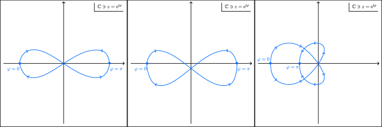
A similar issue shows up in the edge problem, i.e. when restricting the model to a half-space. Then only the longitudinal momentum remains a good quantum number, no matter whether translations are continuous or discrete, at least if the boundary conditions share that symmetry. In the discrete case, however, the range of is compact to begin with and the spectrum is of the form seen in Fig. 2 (first panel): It consists of bands (shaded regions) and curves (in yellow). The energy ranges of the former give rise to the bulk spectrum, collectively in ; not so the latter, which represent the dispersion relations of states propagating along the edge. When considered at fixed , edge states correspond to bound states of .
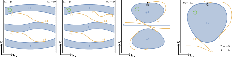
Bulk-edge correspondence [10, 9] relates the Chern number of a band, cf. (2.8), with the mergers of edge states with that band:
| (2.29) |
where is the signed count of states leaving (+), resp. joining (-) the bulk spectrum, as meant w.r.t. the natural orientation of its boundary. That orientation, to be clear, is induced from the one of the plane , see panels of Fig. 2 in green, on the boundaries of the shaded regions. Equivalently, if is taken to run in positive direction, it parametrizes the upper and lower boundary of the band oppositely, as compared to its natural orientation. With that convention,
| (2.30) |
where counts both the edge states leaving the boundary at the bottom and those joining at the top; similarly for .
The second panel of Fig. 2 shows a cancellation between a state leaving and then joining a band. Likewise, such a cancellation should be preserved in the SWM. This, and more, can be achieved by a certain compactification of the -plane, illustrated in panels three and four of Fig. 2. In contrast to Fig. 1, the infinity inside the bulk spectrum is compactified to a single point (the point at infinity ), whereas directions moving to infinity inside the gap, either at or , give rise to a continuum of points at infinity, labeled by , if they attain a horizontal asymptote of that height. In lack of a horizontal asymptote, convergence is to .
So prepared, we may address edge eigenvalues connected to the top band in relation to their behavior in the finite or at infinity. We say:
-
•
An edge eigenvalue merging with that band at finite momentum has a proper merger;
-
•
An edge eigenvalue diverging for has an improper merger;
-
•
An edge eigenvalue having a horizontal asymptote at or has an escape.
Viewed through the compactification, proper and improper mergers look alike, and shall simply be called mergers. We remark that in [19] a somewhat different terminology was used.
Definition 2.8 (Number of proper and improper mergers, number of escapes).
We denote by the signed number of proper mergers, improper mergers and escapes, respectively. Let moreover
| (2.31) |
denote the signed number of mergers.
Let us introduce one last integer of interest. We recall that any (self-adjoint) boundary condition gives rise to a map , with limits . That prompts the following definition.
Definition 2.9 (Boundary winding).
For as above, we call its winding number, i.e.
| (2.32) |
In the next section, our main results are reported, expressed in terms of the integers only. Given our choice of edge index, we set:
Definition 2.10.
Bulk-edge correspondence (BEC) holds true if
| (2.33) |
Accordingly, violations occur for .
Remark 2.11.
Given that the half-space model is determined by the boundary condition, all four integers are functions of just , i.e. , , with
| (2.34) |
Moreover, is a property of , and thus invariant under translations of , cf. Rem. 2.6. Equivalently, is a function of , upon identification of the unitaries that differ by translation of .
3 Overview of results
This section reports the main results of this work and addresses the questions Q1–Q4 raised in the introduction. At first, spectral events that occur while continuously changing the boundary condition will be defined and listed. They are linked to the integers in Defs. 2.31, 2.32, and more properly to their changes. As such, they matter for Question Q3. The number of mergers, cf. (2.31), turns out to be more stable than others, as boundary conditions change; indeed, there is only one kind of change that prevents its invariance. This addresses Q2. The more technical Question Q1 is addressed for its larger part in Sects. 4.4, 5 and App. A. Question Q4 will be dealt with by charting the values of in a phase diagram of boundary conditions. Violations of BEC are typical in all families except for DD, where they do not appear at all.
The first result connects changes in the value of our integers to spectral events, while exploring the manifold of self-adjoint boundary conditions.
Theorem 3.1.
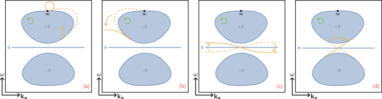
Let the manifold of self-adjoint boundary conditions be partitioned into subsets, or regions, according to the values of , cf. (2.34). They are regular, in the sense that they satisfy . Any transition between regions can be achieved by composition of elementary ones, which occur across boundaries between just two regions, possibly upon arbitrarily small deformation. Transitions are described as follows in terms of spectral events (see Fig. 3):
-
(a)
A merging point reaches or leaves ; as it does so, and change at once, but oppositely: ();
-
(b)
An asymptotically parabolic states turns flat or vice-versa; and change at once, but oppositely: ();
-
(c)
A one-sided flat state disappears from the gap by crossing the zero-energy band, while another one appears at the opposite end; changes, .
Within the above manifold, we single out the exceptional ones, where self-adjointness fails at a point in the sense of Rem. 2.5, and consider an elementary transition across them. Then
-
(d)
On approach, an edge eigenvalue turns vertical at the point of failure; is ill-defined, yet it does not change.
Integers not mentioned in relation to a given event are left unchanged.
Remark 3.2.
The theorem does not rule out further spectral events, not contemplated above, that do not correspond to a transition between level sets of . An example is a simultaneous appearance (or disappearance) of two flat states at opposite ends. Hence .
Remark 3.3.
Within the restricted manifold of boundary conditions corresponding to the particle-hole symmetric case, cf. Def. 2.7, transitions between regions exhibit more than one spectral event, thus failing to be elementary. More than that, the restoration of that property by slight deformation may require that the symmetry is forgone. However, the property of the regions survives the restriction.
An answer to Question Q3 follows as a corollary.
Corollary 3.4.
In plain language, parabolic-to-flat transitions are the only spectral events capable of altering . Regions on the BC manifold where BEC is respected or violated must thus be separated by “surfaces” of type (b) transitions.
Further details on existence and prevalence of BEC are gained by separately charting for all ’s within each of the families DD, ND, DN, NN, starting with DD. In this specific case, no charting is actually needed, as illustrated by the following Proposition.
Proposition 3.5 (Index charts, DD case).
Proposition 3.6 (Index charts, ND case).
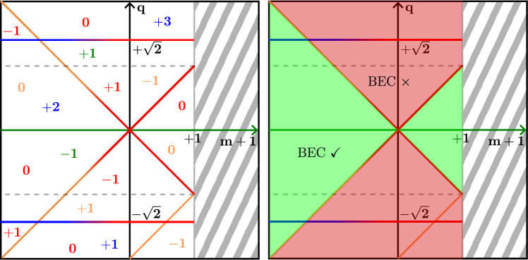
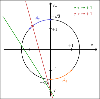
The integer tuple , cf. (2.34), depends on the von Neumann unitary only through some real parameters determined by the boundary condition, whence . A boundary condition is particle-hole symmetric iff . The values of are charted in Fig. 4 (left panel).
Bulk-edge correspondence, namely , is true within the sector
| (3.3) |
(cf. right panel of Fig. 4), and violated outside of it. In particular, BEC is always false on the particle-hole symmetric submanifold .
A comparison with [19] is in order. The boundary conditions of the 1-parameter family considered there are all of type DN and particle-hole symmetric, whence BEC is false throughout that family by our definition. That definition however differs from theirs, which was based on rather than .
In case NN, a graphical representation akin to Figure 4 is not feasible, because of the sheer dimensionality of the associated BC manifold. Yet, restriction to the particle-hole symmetric submanifold makes a drawing possible.
.
Proposition 3.7 (Index charts, NN case with symmetry).
Within the particle-hole symmetric submanifold of NN, depends on only through parameters , whence .
Bulk-edge correspondence, namely , is true within the region
| (3.4) |
and violated outside of it.
Question Q4 is finally answered by specifying a notion of typicality. We say that a property is typical on the manifold of boundary conditions if it holds true with positive measure. The notion is actually proper to the measure class of the Lebesgue measure induced by any local chart.
Theorem 3.8 (Typicality of BEC and violations thereof).
Within the families ND and NN, both BEC and its violation are typical, namely both and its opposite occur on subsets of positive measure.
In summary: Boundary conditions of the family DD exhibit bulk-edge correspondence, but the latter is typically violated in all the other families ND, DN and NN.
In the following sections the above results will be made more precise, e.g. by determining the explicit dependence of on the boundary condition. It is in that version that they will be proven.
4 Details of the setup
4.1 Momentum-space compactification and bulk eigensections
In this section, we review [19] how the odd-viscous regularization enables the compactification of momentum space, mentioned in Sect. 2.1. We moreover provide explicit sections of the bundle of interest, associated to the positive eigenvalue of the bulk model. Such sections are regular everywhere but in a point , hence the superscript.
Above Eq. (2.7), we argued that eigenspaces associated to converge as , thus allowing a compactification of momentum space. That claim is justified below.
Consider the fiber , cf. Eq. (2.4), of the bulk Hamiltonian , cf. (2.2). It can be rewritten as
| (4.1) |
where , and the matrices
| (4.2) |
are an irreducible spin- representation. The fiber shares eigenprojections with its flattened counterpart
| (4.3) |
The eigenprojections read
| (4.4) |
and project onto the eigenspace of , , cf. Eq. (2.5), respectively.
The map is convergent for , and more precisely to
| (4.5) |
thanks to the odd-viscous regularization provided by the term in (4.3). We stress that the limit is attained irrespective of the direction along which is sent to infinity. Accordingly, attains a well-defined limit for , and so do the fibers
| (4.6) |
of the eigenbundle , cf. Eq. (2.8). Along with the 1-point compactification of the plane to the (Riemann) sphere , the Bloch bundle extends as well.
Next, we shift our focus to the eigenbundle of interest, and provide sections that are global except for a single point.
An eigensection of is a smooth map that solves
| (4.7) |
and does not vanish, where defined. We present two eigensections, namely
| (4.8) |
where
| (4.9) |
It is readily verified that they satisfy (4.7). We have
| (4.10) | ||||
because and . Hence, (4.8) extend smoothly to with , respectively. Indeed, and contrary to appearance, is smooth at
| (4.11) |
Likewise,
| (4.12) |
We note that the two patches cover and that the transition function ,
| (4.13) |
has winding , coinciding with as expected.
4.2 Scattering theory of shallow water waves
This section is placed in the context where physical space is the upper half-plane , cf. Eq. (2.12). The scattering of waves at the boundary matters in various ways [19]. In this section, we review how solutions of the edge eigenvalue problem are found as scattering states, namely as linear combinations of incoming, outgoing and evanescent “bulk” waves. At fixed boundary conditions, longitudinal momentum , and incoming transverse momentum , the (unique) scattering solution induces a scattering amplitude , mapping incoming to outgoing waves. Eigenvalues in the discrete spectrum of are found as poles of when analytically continued to the upper half-plane in . The corresponding bound states arise as outgoing (evanescent) waves without incoming counterpart. As varies, the bound states are viewed as edge states of dispersion .
Let a boundary condition , cf. Def. 2.2, be given. Scattering states are obtained as normal modes (2.13) of the formal differential operator , cf. (2.14), that are asymptotic to incoming and outgoing plane waves. In the present context, the transverse momentum is no longer a good quantum number. However, remains a well-defined property of the asymptotic states and , as they are of the form (2.3), and hence determined by their amplitude in . We thus retain a parameter that describes the momenta and of the incoming and outgoing parts, and , respectively. They are related by elastic reflection,
| (4.14) |
because they then share the same frequency, , cf. (2.5).
Moreover, there are two more solutions of , to be found in the analytic continuation of . They are , with in the complex upper half-plane, and are related to by
| (4.15) |
The two solutions are purely imaginary, and correspond to evanescent and divergent waves at , respectively. In particular, participates in the scattering state along with and .
We summarize:
Definition 4.1 (Scattering state).
For and , a scattering state is a solution , cf. (2.13), of and of the form
| (4.16) |
that moreover satisfies the boundary conditions. (The solution exists for every self-adjoint boundary condition , and is unique up to multiples.)
The scattering state (4.16) defines a scattering map, acting between fibers of the eigenbundle in Eq. (2.8), associated to the band :
| (4.17) |
Schematically, the following diagram is commutative:
| (4.18) |
Underlying the definition of is the identification of the amplitudes in with the waves seen in (4.16).
In view of the fact that is nontrivial, sections will have to be local, cf. Sect. 4.1. Let be open subsets equipped with nowhere vanishing sections of . To be clear, and are not required to be subsets of the natural half-spaces (or hemispheres)
| (4.19) |
nor are they required to be related by the reflection ; even less , to be related by (4.17). However, in case and overlap, then a scattering amplitude is defined for by
| (4.20) |
An evanescent amplitude can likewise be defined, by considering an open set of evanescent momenta . The role of the map is now taken by , as in (4.15).
Bound states of the edge eigenvalue problem are now found by analytic continuation in of the scattering amplitude. Provided that the sections above are analytic as well, and turn into exponentially decaying or growing solutions, as . More precisely, is decaying for , and the opposite holds for . The state (4.16) determines a bound state iff none of its terms is diverging in . That criterion is most useful for away from and small , thus exploring a complex neighborhood of the boundary of the bulk spectrum. There, the expression under the square root in (4.15) remains bounded away from zero. Hence the criterion reduces to and . Equivalently, a bound state of energy in the gap occurs iff
| (4.21) |
That amounts to the stance that “bound states are outgoing states with no incoming counterpart”.
4.3 Topological content of the scattering amplitude and bulk-edge correspondence
In the previous section, we introduced the scattering amplitude based on overlapping open sets . Here, we will make more specific choices, such as .
First, however, we take and to be the open set containing the closure of , which thus slightly protrudes into and includes . In particular, form a cover of . Both sets are depicted in Fig. 6, along with a loop running within their intersection and having the same orientation as .
Let be a section on . Then a section is naturally defined on by (4.17),
| (4.22) |
Since and overlap, we may take in the role of in (4.20), and obtain
| (4.23) |
for . Thus
| (4.24) |
there, which exhibits the scattering amplitude as the transition function between local bundle charts of . We conclude the following.
Proposition 4.2 (Thm. 2.7 of [19], first item).
The scattering amplitude , cf. (4.20), relates to the Chern number of by
| (4.25) |
where is any loop as described above.
At the same time, the scattering matrix is sensitive to branches of the discrete spectrum joining the upper band, as illustrated in this version of Levinson’s theorem, originally developed in [14] and later adapted to unbounded Hamiltonians, particularly to the SWM, in [19].
Theorem 4.3 (Levinson’s relative theorem).
Let , and pick (finite) that do not correspond to a merger of an edge mode branch with the bulk spectrum of . Then
| (4.26) |
where denotes a continuous argument and is the signed number of edge mode branches emerging () or disappearing () at the lower band limit between and , as increases.
In simple terms, as we hover over the bottom of the positive band, the phase of jumps by () for each edge eigenvalue leaving (joining) the band. The theorem may be termed as a relative version of Levinson’s theorem [18], since it compares the phases of the scattering matrix at threshold for two values of a parameter (here ), rather than at two ends of an energy interval.
Eq. (4.26) accounts for the part of the winding (4.25) that occurs because of proper mergers. More precisely, we consider a sequence of loops that tend to the “meridian” in the limit , cf. Fig. 6. Let
| (4.27) |
be a partition into two arcs such that converges to the part of the meridian, and to the complementary part containing . For any given boundary conditions, proper mergers do not accumulate at . Thus
| (4.28) |
are well-defined, are integers, and do not depend on , if sufficiently large.
Eq. (4.26) states
| (4.29) |
Recalling Eq. (4.25) and , we moreover conclude
| (4.30) |
Our Def. 2.10 of bulk-edge correspondence, , where is the number of mergers, thus amounts to
| (4.31) |
In other words, violations of BEC occur when the number of improper mergers differs from the winding of at infinite momentum. Such events do occur.
4.4 Details on self-adjoint boundary conditions and particle-hole symmetry thereof
We shall characterize the families DD, ND, DN, NN of self-adjoint boundary conditions (cf. Def. 2.4) and their particle-hole symmetric subsets. Later, in Sect. 5, the main results of the paper will be formulated in the terms introduced here. The proofs of the statements in this section are found in App. A.
Boundary conditions , cf. Def. 2.2, are affine linear maps . As is proven in [19], Lm. B.1-3, and as we shall review in App. A, self-adjointness of , see below Eq. (2.14), imposes various constraints on the entries of the matrix . For short, they are of two kinds, linear and non-linear. Quite generally [41], self-adjoint boundary conditions correspond to subspaces of boundary values , cf. (2.15), that are maximally isotropic w.r.t. some matrix , i.e. .
In the present context, , but the rank of is not maximal, i.e., not , but . This comes about because the deficiency indices of the half-line problem are , rather than as one might instead suspect in view of components of the field and the order 2 of the differential operator (2.2). Note, indeed, that this differential operator is of first order in , but of second in . That accounts for the fact that the matrix can be expressed by a matrix , which solves the linear constraint. The non-linear constraint, now on , comes from the isotropy.
The matrix is related to the by
| (4.32) |
where
| (4.33) |
as shall be justified in App. A. In this new notation, the boundary condition (2.15) is written as
| (4.34) |
By locality of , cf. (2.17), and (4.32), must take the form
| (4.35) |
and we shall also write it as
| (4.36) |
with denoting horizontal juxtaposition and square matrices given by
| (4.37) |
, .
The specific structure (4.35) of the matrix
| (4.38) |
determines the general form of the original boundary condition by
| (4.39) |
cf. (4.33). Note incidentally that the vanishing entry in (4.39) states that no boundary condition involves , as was stated following Def. 2.4, and in line with the above comment on deficiency indices.
By (2.17), the local boundary condition may moreover be written as
| (4.40) |
Comparing Eqs. (4.39, 4.40) then yields
| (4.41) |
The definition of families, Def. 2.4, is a distinction of cases. It affects the matrix only, and thus the vectors , , but not . In the next lemma, we state the implications for . In doing so, we separate the case ND/DN into two, depending on whether is ensured by or .
Lemma 4.4.
The non-linear constraint on remains to be solved. It says:
| (4.43) |
almost everywhere in , see App.A. Equivalently, using (4.36),
| (4.44) |
a.e. in , which is in turn to say
| (4.45) |
cf. (4.37). Those conditions translate into others for , . Remarkably, they amount to real linear equations. The next proposition states them, and in fact separately for the different families of BCs, cf. Lm. 4.4.
Proposition 4.5 (Families of boundary conditions).
We shall also provide an explicit characterization of the particle-hole symmetric (cf. Def. 2.7) subsets of those families.
Proposition 4.6 (Particle-hole symmetric families of boundary conditions).
The map of (4.35) encodes a particle-hole symmetric and self-adjoint boundary condition iff one of the following is true.
-
:
.
-
:
, for some and
(4.49) for some .
-
:
Same as , but with and interchanged.
-
:
linearly independent and
(4.50) for some , and .
We now elucidate how von Neumann unitaries , cf. Def. 2.2, relate to orbits (under left-action of ) of boundary conditions . First of all, notice that and are in one-to-one correspondence, upon imposing self-adjointness. Then, so are their orbits , cf. Eq. (2.16).
The von Neumann unitary associated with orbit (equivalently ) is given by
| (4.51) |
where are as in Eq. (4.36). Eq. (4.51) yields a well-defined map , that descends to a map . The map is moreover one-to-one. These fine points are dealt with in App. A.
As we argued below Eq. (2.16), two representatives of the same orbit encode for the same boundary conditions. The next proposition describes the orbits, and it does so for each family of boundary conditions at a time. Moreover, it does so in terms of the unitaries that are in bijective correspondence with those orbits, cf. Rem. 2.1.
Proposition 4.7 (Families of von Neumann unitaries).
(i) Let be a boundary condition parametrized as in Prop. 4.5 and Lm. 4.4. The corresponding curves in , cf. (4.51), are of the form
| (4.52) |
with depending on families as follows.
-
:
.
-
:
In terms of the parameters and ,
(4.53) -
:
In terms of the parameters and ,
(4.54)
The family DN is obtained by the substitution detailed in Prop. 4.5.
(ii) The particle-hole symmetric subfamilies are given by the same formal expressions, with restrictions on the parameters:
-
:
No changes, DD is always particle-hole symmetric;
-
:
and ;
-
:
, and .
Remark 4.8.
5 Results
In this section, we deepen and extend some of the results of Sect. 3. More precisely, we deepen Prop. 3.6 (ND family) in that we relate the there not yet specified parameters to the more fundamental ones (, ), labeling the boundary conditions of that family; or rather their orbits, which is all that matters, cf. Prop. 4.5 and Prop. 4.7. Likewise, we deepen Prop. 3.7 (NN family) by relating the parameters to the parameters , , labeling the orbits of that family. Moreover, we extend Prop. 3.7, in that we treat all boundary conditions of the family NN, rather than just the particle-hole symmetric ones. As a result, the charts mapping the integer tuple extend accordingly.
By contrast, Prop. 3.5 (family DD) does not require further details. The same applies to other results (Thm. 3.1, Cor. 3.4, Thm. 3.8) spanning across families.
As stated, we begin by rephrasing Prop. 3.6.
Proposition 5.1 (Prop. 3.6, ND family, full statement).
The proof of this result, and of the following one, will be given in Sect. 7.
Remark 5.2.
Prop. 3.7 can similarly be rewritten, moreover considering the entire family NN, rather than its particle-hole symmetric subset.
Proposition 5.3 (Prop. 3.7, NN family, full statement).
Let be a boundary condition in family NN, parametrized as in Prop. 4.5. Let moreover
| (5.6) |
The integers , cf. (2.34), depend only on , and take the following values.
-
•
Let
(5.7) Then
(5.8) -
•
Let
(5.9) The value of stays constant within some regions of parameter space . A first property distinguishing them is the value of , which leads to four tables. Within each of them, further inequalities determine the actual regions. Combinations of inequalities that are empty are denoted by , or are omitted. The values of are listed as entries.
\addstackgap[.5] \addstackgap[.5] \addstackgap[.5] \addstackgap[.5] \addstackgap[.5] \addstackgap[.5] \addstackgap[.5] \addstackgap[.5] \addstackgap[.5] \addstackgap[.5] \addstackgap[.5] \addstackgap[.5] \addstackgap[.5] \addstackgap[.5] \addstackgap[.5] \addstackgap[.5] \addstackgap[.5] \addstackgap[.5] \addstackgap[.5] \addstackgap[.5] Table 1: Values of in different regions within family NN. -
•
Let
(5.10) Then, the values of , for each region of parameter space where it stays constant, are listed in the following table.
\addstackgap[.5] \addstackgap[.5] \addstackgap[.5] \addstackgap[.5] \addstackgap[.5] Table 2: Values of in different regions within family NN.
The winding of the von Neumann unitary , cf. (4.54), takes values as follows. Let
| (5.11) |
Then, if and (general case),
| (5.12) |
By contrast, in the exceptional case where • , • or , and
| (5.13) |
where we recall , then
| (5.14) |
Finally, if
| (5.15) |
or
| (5.16) |
then . In the cases that are not covered, is ill-defined.
Remark 5.4.
Remark 5.5.
Since Prop. 5.3 is an extension of Prop. 3.7, the latter can be recovered from the former by restriction to the particle-hole symmetric subset of family NN. In practice, this is achieved by imposing the constraints on and detailed in Prop. 4.7, point (ii). The thresholds are specialized to PHS, thus becoming
| (5.17) |
Fig. 5 is then recovered by plotting the transition surfaces
| (5.18) |
and decorating each region, defined by such surfaces, with the values of found in the proposition above.
6 Evaluating the integers , , ,
6.1 Number of proper mergers
This section and the upcoming Sects. 6.2, 6.3 and 6.4 illustrate how to calculate each entry of the integer tuple , given a choice of self-adjoint boundary condition, cf. (4.38). Here, we focus on the number of proper mergers , cf. Def. 2.31. In view of the scattering matrix playing the role of a transition function between incoming and outgoing sections of (cf. Prop. 4.2), shall be computed as
| (6.1) |
cf. (4.30), where
| (6.2) |
cf. (4.28), represents the winding of along a contour , entirely contained in a neighborhood of and approximating the meridian of the compactified momentum plane as .
Computing the winding number , and in turn , thus requires: Connecting a self-adjoint boundary condition to its associated scattering matrix ; Expanding the latter around , i.e., the north pole of the compactified momentum plane; Extracting from that asymptotic behavior the winding along . The first two steps, in this very order, are detailed in the paragraphs below. The third point, by contrast, is deferred to Sect. 7.
We start by reviewing [19] how is obtained from a given self-adjoint boundary condition . Recall the definition 4.1 of a scattering state
| (6.3) |
of energy . The scattering and evanescent amplitudes and , cf. Eq. (4.20), allow the following rewriting
| (6.4) |
where sections , of , cf. (2.8), have been chosen, and in particular so that is normalized for all . The expressions for , but not their topological content, depend on the choice of sections.
The scattering amplitude is completely determined by imposing the boundary conditions on the scattering state :
| (6.5) |
cf. (2.15, 4.32). The resulting form of is specified in the next lemma.
Lemma 6.1.
Proof.
We further specialize the choice of sections to
| (6.14) |
cf. (4.8), so as to sit in the case where acts as a transition function of the bundle (see Sect. 4.3 for details). Eq. (6.6) then takes the form
| (6.15) |
where the Jost function is given by
| (6.16) |
with , cf. (6.7), evaluated at
| (6.17) |
Remark 6.2.
Only the first few orders of the expansion of around are relevant for the winding number . We perform that expansion by first bringing to via the (orientation preserving) coordinate change
| (6.18) |
and then expanding around . The leading orders of the resulting series are reported in the next proposition, separately for the families DD, ND, NN of Def. 2.4. As customary, case DN is not pursued, cf. comment right below Def. 2.4.
Proposition 6.3.
The proof of this statement is deferred to App. B.
As the last item of this section, we connect the winding of along the contour appearing in (4.28) to that of along a circumference of fixed radius around the point at infinity .
Lemma 6.4.
Proof.
We split the proof into two parts. First, we claim and prove that the winding of along a certain contour equals the winding of along . Then, we show that and the original contour achieve the same limit as .
Consider, for some , the oriented contour
| (6.24) |
corresponding to a straight line, oriented right to left, in the half-plane of Fig. 7. The winding of along is given by
| (6.25) |
By (6.15), we observe that
| (6.26) |
Then
| (6.27) |
As , the difference of contours becomes topologically equivalent to a positively oriented circle (of small radius ) around the origin of , cf. Fig. 7. Thus,
| (6.28) |
which is the first claim.
For the second part of the proof, we recall that can be any contour, oriented in the direction of increasing , which approximates the infinite portion of the “meridian” as :
| (6.29) |
The candidate contour is thus suitable for the computation of if
| (6.30) |
However,
| (6.31) |
whence the desired limit is achieved by picking . ∎
6.2 Number of improper mergers
In this section, we show how to compute , the number of improper mergers, given the boundary conditions. At first, we notice that is tantamount to the signed number of asymptotically parabolic edge eigenvalues. They correspond to poles of the scattering matrix in a region , of the -plane. There, both evanescent momenta diverge, and it pays to replace them by a point on a Riemann surface. Working on this surface, we express poles of as zeros of , a close relative of the Jost function , cf. (6.15). The required parabolic behavior of the associated edge states imposes the Ansatz , , so that defines a curve in the plane , whose type depends on the families DD, ND, NN of the boundary conditions. Further constraints restrict eigenvalues to lie on certain arcs , of a circle in the -plane, and the value of is thus geometrically found as the signed number of intersections between the curve and the arcs.
Above Def. 2.31, was defined as the signed number of edge eigenvalues diverging for . Such eigenvalues are asymptotically quadratic in : Faster divergences would make the eigenvalue hit the positive bulk band at finite , whereas slower ones would imply that the eigenvalue and band edge never actually meet. The problem of finding thus reduces to identifying all asymptotically parabolic edge eigenvalues , and counting them with sign. More precisely, this section considers a region
| (6.32) |
of the -plane, meaning for any fixed . Other regions, for example will be considered later.
As discussed above Eq. (4.21), the edge states of interest shall be found as solutions, in , of
| (6.33) |
at , moreover with energy
| (6.34) |
lying in the desired region (6.32) and . Those edge states involve two evanescent states of rates that determine each other, cf. (4.15). In the regimes (6.32) they will both diverge and it pays to treat them on the same footing.
Fix and ignore for the time being. Let be the two solutions, in , of
| (6.35) |
namely
| (6.36) |
where we stress that by (cf. comment below Eq. (2.1)). The solutions are related by Vieta’s formulae
| (6.37) | |||
| (6.38) |
A convenient way to view these equations is as follows. Eq. (6.35) determines a map with for real. For , we moreover have
| (6.39) |
Conversely, pairs are constrained by (6.37), one of Vieta’s formulae, and is then determined by the other. By extension, determine by
| (6.40) |
We thus find
| (6.41) |
up to signs. Notice that iff , a condition equivalent to sitting in a spectral gap: , cf. (2.6). By contrast, is granted, even outside of the spectral gap, by , , cf. (6.36). Moreover,
| (6.42) |
Again and conversely, we consider points , where are constrained by (6.40, 6.37) and is determined by (6.38). Eq. (6.40) allows for two branches of each. At first we shall not distinguish between them, thus viewing as a point on a Riemann surface depending on .
We now consider functions on that surface, such as the scattering amplitude whose poles we wish to identify, cf. (6.33). We moreover discuss such zeros only in the generic case where the index is well-defined. That entails that all the fibers are self-adjoint one by one, cf. Rem. 2.5, and actually including at in a natural sense. In turn, that means that the Jost functions , related to by (6.15), have an easily identifiable asymptotics at . It allows to simplify the quotient
| (6.43) |
in favor of simpler expressions , that are found, for families DD-ND-NN, as follows. The expansions of Prop. 6.3 are still formally valid, upon replacement , because was there explored along a parabola , cf. central panel of Fig. 6, that lies within the region , here under study. However, there because was in the bulk band; here, because is chosen in the gap. The desired ’s are obtained, family by family, from those expansions by retaining the leading orders only and performing the simplifications alluded to in (6.43).
Proposition 6.5.
Proof.
We start by retaining the leading order in of the expansions (6.19):
| (6.45) |
We pass to a notation in terms of by
| (6.46) |
This results in
| (6.47) |
By the assumption of self-adjointness at infinity, equivalently well-defined there, the prefactors , , are non-zero in family DD, ND and NN, respectively. They can thus be simplified in the spirit of (6.43), leading to the expressions of listed in (6.44). ∎
For all families DD-ND-NN, is homogeneous in . This prompts the Ansatz
| (6.48) |
with , for solutions of at . The parameters are constrained by consistency with (6.35, 6.40). In particular, solutions of (6.35) are related to one another by the first Vieta formula, cf.(6.37),
| (6.49) |
At , the above and our Ansatz imply
| (6.50) |
Moreover, at , Eq. (6.39) is rewritten, through (6.40) and in terms of our Ansatz, as
| (6.51) |
from which the further constraint
| (6.52) |
Finally, the branches corresponding to bound states have , namely , (, ) at (). All in all, asymptotically parabolic edge eigenvalues at , or , are found as points belonging to the algebraic variety
| (6.53) |
and additionally satisfying the constraints
| (6.54) |
for , or
| (6.55) |
for .
Solutions of correspond to curves in the -plane, differing between families DD-ND-NN as detailed in the lemma below.
Lemma 6.6.
The task of computing the number of improper mergers was thus reduced to counting the intersections (with sign) of the curves of Lm. 6.6 with the arcs . By the conventions illustrated in the third and fourth panel of Fig. 2, intersections with (), corresponding to parabolic bound states at (), contribute () to the total number of improper mergers. In summary,
| (6.59) |
The value of in the families DD-ND-NN will be computed in Sect. 7, making use of (6.59).
6.3 Number of escapes
This section is similar to the previous one, in that we find edge states at as zeros of the Jost function . It however differs from it, because we require , . Since this regime has very small overlap with that of Sect. 6.2, cf. (6.32), the expansions thereby found for are generally not valid. With no assumptions other than , whence also by (6.35), we expand around , and study the zeros of its leading order for different behaviors of . If as , is true only exceptionally in the space of boundary conditions. By contrast, asymptotically flat solutions at are typical. The height of those asymptotes is separately computed and listed for families DD, ND and NN.
Like in the previous section, we wish to find solutions with of
| (6.60) |
at , corresponding to eigenstates of energy
| (6.61) |
Moreover, we again see as a function on the Riemann surface of , cf. (6.40). Unlike before, however, we focus on edge eigenvalues such that
| (6.62) |
This region only slightly overlaps (6.32). The union of the two is moreover the whole -plane, ensuring that we explore all of the gap. Again in contrast with the previous section, we fix the branches of that grant from the very beginning:
| (6.63) |
Consider as in (6.35). By (6.62), we have
| (6.64) |
whence
| (6.65) |
Since the regions (6.32) and (6.62) have a large symmetric difference, we cannot rely on the expansions of Sect. 6.2 to determine poles of at , corresponding to edge states. We thus proceed as follows.
Eq. (6.15) allows looking at zeros of the Jost function , rather than at poles of . The condition (6.62) on is enforced by expanding around , and retaining the leading order. Within it, we then look for zeros at . These turn out to change depending on the asymptotic behavior (in ) of , and we thus find it advantageous to read as an implicit equation for rather than , cf. discussion below Eq. (6.42). If , has solutions only exceptionally in the space of boundary conditions. By contrast, if at , solutions of exist almost everywhere in the space of BCs. These claims are formalized in the next proposition, where we also provide the values of the horizontal asymptotes, separately for each of the families DD, ND and NN.
Proposition 6.7.
In the interest of readability, the proof of this result is deferred to App. C.
Computing the number of escapes , given some boundary conditions, was thus reduced to the following counting exercise. A flat asymptote of height () at () contributes () to . This convention comes about by consistency with the counting of parabolic states, cf. Fig. 2. By contrast, eigenvalues give no contribution to , because they do not pertain the positive bulk gap of interest. In summary,
| (6.73) |
The value of stemming from (6.73) is displayed, for each of the families DD, ND, NN, in Sect. 7, and leads to the proof of Eq. (5.4) in Prop. 5.1 and Tab. 2 in Prop. 5.3.
6.4 Boundary winding
In this section, we discuss how to compute the winding number (dubbed boundary winding, cf. Def. 2.32) of the unitary associated with a given orbit of self-adjoint boundary conditions. Generally, Prop. 4.5 holds, and computing amounts to applying formula (2.32). However, there exist exceptional (as in, atypical in the sense of Thm. 3.8) boundary conditions, where takes values that differ from those given by the integral formula (2.32) applied to (4.53), (4.54). Below, we tackle both general and exceptional cases. In the interest of readability, most proofs are deferred to App. D.
Recall that
| (6.74) |
cf. (4.51, 4.36). Observe moreover that describes a curve in the complex plane. Its winding about the origin, which we denote by , is such that
| (6.75) |
as is seen by (2.32) and
| (6.76) |
for any unitary in . By known properties of winding numbers and (6.74)
| (6.77) |
where . Moreover, by the affine linear structure of
| (6.78) |
is a polynomial of order (at most) two in , namely a parabola. For the exceptional boundary conditions mentioned in the introductory paragraph, the parabola however degenerates to a line, or even a single point in the complex plane .
Before computing for boundary conditions in families DD, ND, NN (cf. Def. 2.4), let us lay down general formulae for the winding of a (possibly degenerate) parabola
| (6.79) |
where , around the origin of its complex plane. Let
| (6.80) |
and
| (6.81) |
These quantities are of importance in the lemmas below.
Lemma 6.8 (I: Curve traced).
The curve , traces out
-
(a)
a point, if ;
-
(b)
a straight line, if , ;
-
(c)
a half-line traced both ways if , ;
-
(d)
a parabola, if otherwise; i.e., if , .
In each case, the converse also applies.
Lemma 6.9 (II: Avoidance of origin).
The conditions for
| (6.82) |
are, depending on the above cases,
-
(a)
;
-
(b)
;
-
(c)
• , or • and
(6.83) -
(d)
.
Remark 6.10.
Ad (c): In the second case, both sides of (6.83) are real by , .
If the origin is avoided, cf. (6.82), the winding number about is defined in the obvious (counter clock-wise) sense. It takes a half-integer value if the curve happens to be a straight line.
Lemma 6.11 (III: Winding about origin).
If the conditions I, II are met, the winding number is
| (a) | ||||||
| (b) | (6.84) | |||||
| (c) | ||||||
| (d) | (6.85) |
The next lemma connects the coefficients of to the boundary conditions of interest.
Lemma 6.12.
Proof.
The lemmas above, starting with the last one, can now be specialized to the families DD, ND, NN of boundary conditions, cf. Def. 2.4. As customary, DN is not treated because of the substitution detailed in Prop. 4.5.
Lemma 6.13.
When spelled out for families DD, ND, NN, Eq. (6.86) reads
-
DD:
(6.89) -
ND:
(6.90) -
NN:
(6.91)
Proposition 6.14 (Boundary winding , family DD).
Proof.
Eq. (6.77) applies. By we have , whence , whenever one of them (and hence both) are well-defined. Thus follows. ∎
The just stated result for family DD does not come as a surprise, since is a constant, cf. Prop. 4.7.
Family ND is of greater complexity. There, Eq. (6.90) implies
| (6.93) | ||||
The first factor in the last member of the equation above does not contribute to the winding by
| (6.94) |
Its zeros are however of relevance when discussing avoidance of the origin. In fact, we shall show that have no zeros , implying that crossings of the origin, and in turn failure of self-adjointess, only take place at the fiber solving
| (6.95) |
cf. Lm. A.7 for details. We thus focus on only, and in fact only on the variant, dropping subscripts. The variant is recovered by the replacement
| (6.96) |
Below,
| (6.97) |
shall be seen as a special case of (6.79) with
| (6.98) | ||||
whence and
| (6.99) |
Proposition 6.15 (Winding of , family ND).
Let be a self-adjoint boundary condition in family ND, cf. Def. 2.4, moreover parametrized as in Lm. 4.4, Prop. 4.5. Then, the polynomial , cf. (6.97), satisfies:
I. (Curve traced) The curve traces out
-
(a)
a point iff ;
-
(b)
a straight line iff .
II. (Avoidance of origin) Depending on the cases in I, the curve avoids the origin, cf. (6.82), according to
-
(a)
always;
-
(b)
always.
Proof.
We now present the specialization of Lms. 6.8, 6.9, 6.11 to family NN. Just like in case ND, we focus on . Analogous results for are recovered via the substitution detailed prior to the proof of the next proposition, which shall be found in App. D.
Proposition 6.16 (Winding of , family NN).
Let be a self-adjoint boundary condition in family NN, cf. Def. 2.4, moreover parametrized as in Lm. 4.4, Prop. 4.5. The polynomial
| (6.101) |
with , as in (6.91), satisfies:
I. (Curve traced) The curve traces out
-
(a)
a point iff ;
-
(b)
a straight line iff • and • ;
-
(c)
a half-line traced both ways iff • and • or ;
-
(d)
a parabola iff and .
II. (Avoidance of origin) Depending on the cases in I, the curve avoids the origin, cf. (6.82), according to
-
(a-d)
always.
7 Proofs of the main results
In this section, we provide proofs of the main results. We start with Prop. 3.5, reporting the value of the integer tuple , cf. (2.34), on the single orbit making up family DD. It is shown as a direct consequence of the preparatory results Props. 6.3, 6.5, 6.7, 6.14. We then proceed to prove Props. 5.1 and 5.3, concerning the values of within families ND and NN. The first (second) one immediately implies the “index map” of Prop. 3.6 (Prop. 3.7). Jointly, the two also imply Thm. 3.8 on typicality of bulk-edge correspondence and lack thereof. They are moreover essential in showing Thm. 3.1 on the kinds of transitions of , and their relation to spectral events. Thm. 3.1 in turn implies Cor. 3.4 on the mechanism for violation of bulk-edge correspondence.
We follow the program above, and start by discussing Prop. 3.5.
Proof of Prop. 3.5.
The proposition consists of two statements. The first one is that
| (7.1) |
where denotes Dirichlet boundary conditions. They are in DD because they involve no derivatives, cf. Def. 2.4, or equivalently because their matrix form is
| (7.2) |
cf. (2.22) and (4.32), whence and by Lm. 4.4. Moreover, DD consists in a single orbit, namely
| (7.3) |
by Prop.(4.7). Thus, holds true for all .
The second statement is that
| (7.4) |
on the single orbit labeled by . We proceed entry by entry.
Number of proper mergers . We argued in Sect. 6.1 that is obtained as
| (7.5) |
where is the winding of the scattering amplitude in a neighborhood of (i.e., ). However, by Eq. (6.19),
| (7.6) |
at leading order, whence and
| (7.7) |
Number of improper mergers . By Eq. (6.59), this integer is the signed number of intersections of the curve , implicitly defined by
| (7.8) |
with , , cf. (6.54, 6.55). However, by (6.44),
| (7.9) |
and the curve is empty. Thus,
| (7.10) |
Number of escapes . Two asymptotically flat states exist, with asymptotic height
| (7.11) |
cf. (6.66). By formula (6.73),
| (7.12) |
Boundary winding . The value of was found in Prop. 6.14, and reads . ∎
For the proofs of Props. (5.1, 5.3), we recall a few notions. The first one is that of orbit parameters. The parametrization proposed in Prop. 4.5 for the families DD-NN, cf. Def. 2.4, is redundant if the object of interest are orbits under action, rather than single BCs . We call orbit parameters those that survive the lift . In practice, they are the ones explicitly appearing in the von Neumman unitary labeling the orbit, cf. Prop. 4.7. Even orbit parameters are partly redundant when concerned with global properties of the edge Hamiltonian , due to the freedom in reparametrizing , cf. Rem. 2.6. Parameters invariant under this freedom are called genuine. Concretely, those are in family ND, and in family NN, cf. Rems. 4.8, 5.2, 5.4. The discussion does not apply to DD, since a single orbit is parametrized by a single, constant parameter. Genuine parameters are unconstrained, and were chosen real. We thus call the parameter space of ND or NN or , respectively.
Alongside these notions, we shall use the following argument several times. Let be a -valued function. Let be continuous everywhere except on a finite number of transition surfaces, namely manifolds in of codimension one, implicitly defined by
| (7.13) |
for some . The function is uniquely characterized by the (transition) surfaces where it changes, and its value in the regions that have those surfaces as boundaries. A transition surface like (7.13) partitions parameter space in two regions
| (7.14) |
In presence of a second surface , would overall be partitioned in four regions, identified by the four ways of combining and . The reasoning generalizes immediately to an arbitrary number of transition surfaces. The value of in a region where it is constant is simply found by evaluating for some .
As observed in Rem. 2.11, the integers are global properties of , and they hence depend on genuine parameters only. They are moreover piece-wise constant functions ( for ND, NN respectively), and the above characterization applies.
Remark 7.1.
Recall Eq. (6.23):
| (7.15) |
where . If the winding of is well-defined, then it is stable in and provides . That need though not be the case, and in fact when occurs for some . The latter will turn out to be the case in family ND, but not in NN.
Proof of Prop. 5.1.
We discuss the entries of the integer tuple one by one. Throughout the proof, we shall assume . By continuity, the assumption can be dropped.
Number of proper mergers . The winding of is not well-defined, cf. Rem. 7.1, and does not dispense from computing that of . We will nonetheless consider first. The winding of is unchanged when replacing , whence by (6.19), and dropping primes,
| (7.16) |
This means
| (7.17) |
We note that
| (7.18) |
and that
| (7.19) |
with
| (7.20) |
having . In Fig. 9, left panel, we draw assuming .
Let
| (7.21) |
We note the invariance of under , cf. Rem. 2.6, since it changes only the real part of the product. For now, let .
The curve in the figure visits the origin both at . We claim it avoids it for small , and in fact as shown in Fig. 9, center panel. The winding then vanishes. In order to establish this, we consider at first order near , i.e., for small :
| (7.22) |
namely
| (7.23) |
cf. (7.20). Notice the invariance of the line (up to reparametrization) under the usual reparametrization of .
We keep for now. Then the line for runs to the left of that for , provided they are oriented according to increasing . That is the case near , but not near . Correspondingly, the origin will be found to the right of near (respectively, left near ). That confirms Fig. 9, center panel.
Though has the curve move to the other side of the origin, the winding around it still vanishes. The same conclusion holds for . It remains to be seen what happens when , are of opposite signs, starting with as in Fig. 9, right panel. The local situation near the origin is as above, and the same avoidance occurs at . The winding number of equals . A similar picture for yields the winding number . In summary,
| (7.24) |
Case has been omitted because impossible: At least one in , must be negative by , cf. (7.19).
It remains to rephrase the cases as in (5.2). The condition is rephrased as
| (7.25) |
namely , using the definition (5.1) of . Similarly, is equivalent to . Finally, is rephrased as . This concludes this part of the proof.
In closing, we highlight that has two transition surfaces, namely
| (7.26) |
where is given as a function of the genuine parameters in (5.1).
Number of improper mergers . We count intersections of
| (7.27) |
cf. Eq. (6.57), with and , cf. (6.54, 6.55). Their signed number determines through (6.59), and is a piece-wise constant function on parameter space. We thus characterize it by: (a) its transition surfaces; (b) its value in regions that have those surfaces as boundaries.
(a) Let
| (7.28) |
denote the edge points of the target arc (). The number of intersections of with only depends on the curve’s height at , namely on the value of and . Since are continuous functions, the number of intersections only changes when the edge points are met, i.e.
| (7.29) |
Similarly, the number of intersections with changes at
| (7.30) |
No transition surface other than (7.29, 7.29) exists, and regions are defined by picking
| (7.31) |
and one alternative for each of these two inequalities:
| (7.32) |
Some of those regions are empty, and do not appear in Eq. (5.3). For example, implies by , and is thus incompatible with .
(b) Consider for example and . The third inequality is necessarily , or equivalently , due to and . Geometrically, cf. Fig. 10, the three inequalities mean
| (7.33) |
whence the line avoids both and , i.e., .
By contrast, if and ( still), we have
| (7.34) |
The arc is intersected while is still avoided, whence by (6.59).
Repeating the analysis for all non-empty regions yields (5.3).
Number of escapes . As per (6.73), we have to count the number of horizontal asymptotes of positive height, encoded by Eq. (6.69):
| (7.35) |
Zeros of , , identify the transition surfaces
| (7.36) |
respectively. More precisely, the numerator is positive for
| (7.37) |
The denominators are positive for
| (7.38) |
As a consequence,
| (7.39) |
and
| (7.40) |
Eq. (5.4) follows.
Boundary winding . Notice that iff and . If , point III (a) of Prop. 6.15 implies , by
| (7.41) |
cf. (6.94), and the fact that both trace a single point. By contrast, if both trace a line. Eq. (6.100) then states
| (7.42) |
The variant is recovered by the replacement (6.96):
| (7.43) |
Thus,
| (7.44) |
as claimed in Eq. (5.5). ∎
Proof of Prop. 5.3.
Number of proper mergers . Like in the previous proof, we start by inspecting . In fact, since its winding is identical to , and in family NN, we inspect the latter (while calling it all the same). By Eq. (6.19), it reads
| (7.45) |
where
| (7.46) | ||||
The origin of the complex plane is met for no , if not for exceptional values of the parameters , . There is thus no need to consider the full Jost function , , cf. Rem. 7.1.
The winding number of a loop , , about the origin is completely determined by: The number of intersections with the real axis, , ( some index set); The position of relative to each other and zero; The orientation of the curve. We exhibit the data above for , as a function of the parameters, upon noticing that
| (7.47) |
allows us to study only.
Zeros of are: • for all ; implicitly given by
| (7.48) |
if solutions to this equation exist. Since the l.h.s. has range , that is the case for
| (7.49) |
cf. (5.6) for the definition of . We moreover notice that if and if .
The orientation is fixed by specifying for some , e.g.
| (7.50) |
At the intersection points, the value of is
| (7.51) | ||||
| (7.52) | ||||
| (7.53) |
cf. (5.6, 5.7). Notice that , whenever exists as a solution of , namely when .
The winding number of is thus uniquely fixed if we specify a region with the following (candidate) transition surfaces as boundaries
| (7.54) |
Let us inspect one such region. The others are in all respects analogous.
• and .
To make contact with Eq. (5.8), we rephrase the constraints in the notation of that equation:
| (7.55) |
whence we sit in case
| (7.56) |
Drawing a curve according to this data, cf. left panel of Fig. 11, reveals
| (7.57) |
Repeating the reasoning for all cases, some of which actually correspond to empty regions in parameter space, leads to the following table, whose entries represent values of in a given region.
| \addstackgap[.5] | ||||
|---|---|---|---|---|
| \addstackgap[.5] | ||||
| \addstackgap[.5] | ||||
| \addstackgap[.5] | ||||
| \addstackgap[.5] | ||||
| \addstackgap[.5] | ||||
By inspection of this table,
| (7.58) |
were, in hindsight, not transition surfaces. Eq. 5.8 follows.
Number of improper mergers . The curve whose intersections with yield is now a hyperbola. More precisely,
| (7.59) |
cf. (6.58) and (5.6), where represents a point in parameter space (the genuine parameter is not reported, since it does not appear). Two facts will be important in the following. First, the center of the hyperbola lies at
| (7.60) |
Second, the hyperbola always sits in the first and third quadrant w.r.t. its (horizontal and vertical) asymptotes, namely
| (7.61) |
Like in the previous proof, we determine by: (a) identifying its the transition surfaces; (b) evaluating it in each region with the transition surfaces as boundaries.
(a) Once again, the number of intersections of the hyperbola with only depends on its height at , namely on the value of and . If were continuous functions, like in family ND, the number of intersections would only change when the edge points are met, i.e.
| (7.62) |
However, such functions are discontinuous for , namely
| (7.63) |
Jumps in the number of intersections with must occur across the transition surfaces (7.62), and could occur across (7.63).
Similarly, the number of intersections with may jump at
| (7.64) |
(the transition is shared with ).
A region whose boundaries are transition surfaces is thus specified by picking
| (7.65) |
and one alternative
| (7.66) |
for each . This entails a grand total of regions, an example of which could be
| (7.67) |
The tally can be lowered to the forty-eight cases of Tab. • ‣ 5.3 by observing that
| (7.68) |
As a consequence, picking and or at once would specify an empty region. The choice of is still free, so this rules out cases. Out of the remaining , another are similarly eliminated by
| (7.69) |
(b) Given a region as specified above, we evaluate by simply picking , drawing , and counting its signed number of intersections with the target arcs. Consider for example , cf. 7.67. The constraints geometrically read
| (7.70) |
for all , upon noticing that is equivalent to
| (7.71) |
to
| (7.72) |
and to
| (7.73) |
A representative curve is drawn in Fig. 11.
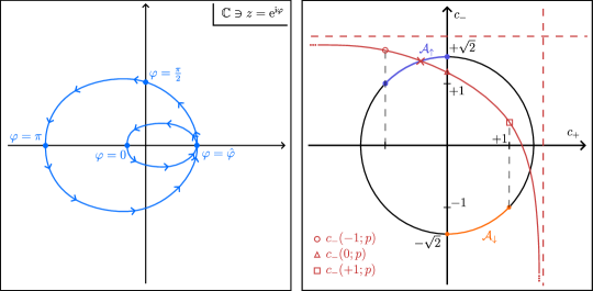
By and the constraints (7.70), the lower branch of the hyperbola intersects and avoids . By (6.59), the only intersection with contributes , whence
| (7.74) |
Similar counting for the other 47 regions provides the entries of Tab. 1.
Number of escapes . Just like in the proof of Prop. 5.1, we need to count the signed number of positive horizontal asymptotes. This time,
| (7.75) |
cf. Eq. (6.72). changes across the transitions surfaces
| (7.76) |
cf. (5.10), and
| (7.77) |
The last two were already encountered in the discussion of .
Tab. 2 now stems from observing that for
| (7.78) |
and recalling that () contributes () to , or zero otherwise.
Boundary winding . As far as is concerned, Prop. 5.3 is a mere restatement of Prop. 6.16, if not for the fact that
| (7.79) |
is reported explicitly. Recall (6.102), which says (re-instating subscripts)
| (7.80) | ||||
cf. (5.6, 5.11). The variant is obtained via the replacement (D.6). It entails , , , whence
| (7.81) |
and
| (7.82) |
This completes the proof. ∎
Proof of Prop. 3.7.
Follows by specializing Prop. 5.3 to the particle-hole symmetric subcase of family NN, via the restrictions detailed in Prop. 4.6. In particular, (4.50) demands , and the new transition manifolds are found by
| (7.83) |
Notice that , cf. also (5.17). Two transition manifolds of come to coincide when restricted to the particle-hole submanifold within family NN. As a consequence, undergoes a non-elementary transition while crossing , cf. Thm. 3.1 and Rem. 3.3. This is displayed in Fig. 5, where crossing yields . ∎
Proof of Thm. 3.8.
In family DD, there is no notion of typicality, since it consists in a single orbit. In family ND, typicality of violations (or not) of bulk-edge correspondence is already evident from Fig. 4. In family NN, inspection of (5.8) and Tab. 1 reveals that
| (7.84) |
namely bulk-edge correspondence holds, for . Conversely, it is violated in the complementary case. The proof is concluded by noticing that both sets are positive-measure. ∎
Proof of Thm. 3.1.
We divide the proof in two parts, (i) and (ii). In (i), we argue, based on Props. 5.1 and 5.3, that the entries of , cf. 2.34, only change in the specified combinations (a)-(d). In (ii), we connect such changes to spectral events.
-
(i)
Relations between transitions of integers.
-
(a)
The claim is , and that does not change otherwise. Both facts are trivially true in family DD, where parameter space is a point and no transitions exist. We analyze ND and NN separately, while DN is recovered from ND by the substitution detailed in Lm. 4.4.
ND: Transitions of only happen at
(7.85) cf. Eq. (5.2). As a consequence of Eq. (5.3), they are shared by . When () is crossed in direction of increasing ,
(7.86) by Eq. (5.2) or Fig. 4. At the same time,
(7.87) proving this part of the claim.
NN: By Eq. (5.8), transition surfaces of are
(7.88) They are shared by , cf. Tab. 1. Inspection of Eq. (5.8) and Tab. 1 allows checking within each of the regions defined by the boundaries
(7.89) and
(7.90) The statement is seen to hold true while crossing , for each such region separately, and thus generally for family NN.
-
(b)
The claim is that there exist transitions where change jointly, and in that case . Family DD is again trivial, and will be omitted from now on. In families ND and NN, the transition surfaces of that are not shared with are however shared with . They read
(7.91) in the former family, cf. (5.3), and
(7.92) in the latter. That while crossing the aforementioned surfaces follows from inspection of Fig. 4 in family ND, and of Tabs. 1, 2 in family NN. In the latter case, comparing the two tables is actually not immediate, and requires careful ordering of the surfaces in direction of increasing .
-
(c)
In family ND (NN), has a single transition surfaces
(7.93) not shared with other indices, cf. Eqs. (5.4, 5.10). That while crossing them is read by Eq. (5.4) (family ND), or by subtracting the two columns of Tab. 2 (family NN) along the rows where . In the rows with , passing from one column to the other does not constitute, by the definition of Thm. 3.1, a transition of . Incidentally, we notice that this move across columns with is associated to the spectral event discussed in Rem. 3.2.
- (d)
-
(a)
-
(ii)
Correspondence with spectral events.
-
(a)
Levinson’s relative theorem, cf. 4.3, establishes a correspondence between and the signed number of mergers with the bulk spectrum. If changes, one such merger must appear of vanish. By continuity of edge eigenvalues in , such mergers cannot appear or disappear at will, but must rather be drawn from, or repelled to, infinity. Hence the claim.
-
(b)
In families DD (trivially), ND and NN, the only typical asymptotic behaviors of edge eigenvalues are parabolic, (cf. (6.32)), or flat, , , cf. Eqs. (6.66, 6.69, 6.72). This fact is seen as follows. Parabolic behavior is typical because edge states with exist at in positive-measure subsets of ND, NN, cf. Props. 5.1 and 5.3. By now considering at , we cover the entire -plane. In this region, Prop. 6.7 proves that the only typical behavior is asymptotically flat. Different asymptotic behaviors , , are admitted only exceptionally, and more specifically only on the transition surfaces of , cf. (6.67, 6.68, 6.70, 6.71).
If , a parabolic state is lost and a flat one gained, or vice-versa. Due to continuity and the typicality statement above, the loss and gain shall be ascribed to the same edge state turning from parabolic to flat, or vice-versa.
-
(c)
If alone changes, the transition involves asymptotically flat states only. At , there can be at most one flat state at a time, cf. (7.75). These two facts, combined with , cf. point (i), lead to the only logical conclusion that two asymptotes, one at and the other one at , cross zero in opposite direction.
-
(d)
This case is different from the other one, in that the transition is not characterized by a change in , but rather by loss of self-adjointness. This is to say, at transition there exists at least one such that the boundary conditions , cf. (4.38), have
(7.94) We shall assume that exactly one such point exists, because the extension to finitely many (or even a countable infinity of) points is immediate.
With this simplifying assumption, the claim has become that, if (7.94) holds, then
(7.95) and is ill-defined, yet it does not change while crossing the BC .
We prove the claim on the spectrum first. Since
(7.96) cf. Eq. (2.6), we need only prove
(7.97) Let (namely, in the gap) and let be such that . Then, a candidate eigenstate of energy is the scattering state , with
(7.98) cf. (4.16) with some choice of normalized bulk sections , . W.l.o.g., we can set , just like we set in Eq. (6.4), while defining the scattering amplitude . The scattering state satisfies the given boundary conditions iff
(7.99) cf. (6.5). We rearrange this equation as
(7.100) By Cramer’s rule,
(7.101) By hypothesis, , whence
(7.102) The resulting state
(7.103) thus satisfies the boundary conditions, at , for all in the gap, or equivalently all s.t. . It is moreover in by . This concludes this part of the proof.
To prove the claim on , we recall (6.77):
(7.104) where is the orbit of , denotes the winding number of a curve , and
(7.105) cf. (6.74) and (4.36). By Claim A.5
(7.106) Thus, iff
(7.107) namely loss of self-adjointness is equivalent to both curves crossing the origin, in which case is ill-defined. This is the first claim. The second one is that does nonetheless not change in value, when crossing a locally non self-adjoint BC. We prove the statement family-wise. It is trivial in DD, so we focus on ND and NN. In ND, loss of self-adjointness occurs at the single (if existent) solution of
(7.108) cf. (A.86). It however produces no change in , due to (6.93). In NN, all boundary conditions are everywhere self-adjoint, cf. Lm. A.7 and Rem. LABEL:rem:d21NeqZero, and no transitions in the sense of this point thus occur.
-
(a)
∎
Proof of Cor. 3.4.
Since bulk-edge correspondence was defined as , cf. Def. 2.10, only a change in or can alter its status. However, is a constant, independent of boundary conditions. Thus, is the only possible violation mechanism. Out of the allowed transitions (a)-(d) of Thm. 3.1, only those of type (b) produce
| (7.109) |
whence the claim. ∎
8 Acknowledgements
The authors heartily thank J. Kellendonk for numerous illuminating discussions, especially on the role of von Neumann unitaries, and C. Tauber for his careful reading of the manuscript and valuable remarks. They moreover thank G. C. Thiang and again C. Tauber for discussions at an early stage of the work.
Appendix A Further facts on boundary conditions
This appendix recalls the results of [19] on self-adjointness of boundary conditions , cf. Def. 2.2, previously displayed in Sect. 4.4. Next, a proof is provided for Lm. 4.4 and Props. 4.5, 4.6, 4.7. We later turn our attention to failure of self-adjointness at a single fiber , signaled by failing to be maximal rank. Whether a boundary condition is maximal rank a.e. or everywhere in is the question tackled in Prop. A.7 below.
As anticipated, we start by reviewing the formalism and results of [19]. Recall Eq. (2.15): A scattering state , cf. (4.16) in Def. 4.1, satisfies the boundary condition if
| (A.1) |
where and
| (A.2) |
as per Eq. (4.35). The matrix has precisely two rows because two equations suffice to uniquely identify a solution of , cf. Eq. (2.14). On the other hand, one equation is not enough, so that
| (A.3) |
a.e. in . Differently put, all self-adjoint boundary conditions are represented by matrices of maximal rank.
It is proven in [19] that a given BC , cf. again Def. 2.2, encodes for a self-adjoint realization of the formal differential operator if and only if
| (A.4a) | |||
| (A.4b) | |||
almost everywhere in . Equivalently, cf. (A.2),
| (A.5a) | |||
| (A.5b) | |||
Eq. (A.5a) implies that two out of the six columns of are redundant, so that one may generically write
| (A.6) |
where and denotes the horizontal juxtaposition of two (or more) matrices. This is to say, if is an and is an , is an built up by “gluing” to the right of . Eq. (A.6) is equivalent to (4.39), whence our claim (4.41) on the general form of follows.
The structure (A.2) of , with only four independent columns, prompts the simpler rewriting as a matrix
| (A.7) |
and the matrix of (4.33) is read off by direct comparison of with , cf. (A.6, A.7).
Any BC , with as in Eq. (A.7), satisfies (A.5a) by construction. On the other hand, (A.5b) is yet to be imposed on . Again by , it translates to
| (A.8) |
almost everywhere in , where
| (A.9) |
the second identity following from Eqs. (4.33, A.4b) and matrix multiplication. By (A.8), we have thus recovered (4.43).
Proof of Lm. 4.4.
Recall Eq. (4.41), namely
| (A.10) |
Then
-
DD:
iff , i.e. , ;
-
NN:
iff , i.e. , linearly independent.
If , there exists an invertible matrix
| (A.11) |
with and l.i. , such that
| (A.12) |
has one row equal to zero (w.l.o.g. , the second one), where denotes inner product in . If the second row is zero, in , and thus , i.e. , linearly dependent.
The further distinction between ND and DN arises as follows. Since is l.i. from and non-zero, the inner products appearing in the first row are only zero for or , respectively. If a term in persists in the BC after elimination of the second row, it means that the , whence and thus . This characterizes family ND. Family DN is obtained in the same way, requiring to persist. ∎
Prop. 4.5 reduces to two simpler propositions by means of the following reasoning. The condition to be met is
| (A.13) |
a.e. in , cf. (4.44). Recall the decomposition , cf. (4.37). If one lets , then
| (A.14) |
The l.h.s. of (A.13) can be rewritten as
| (A.15) |
and it equals zero a.e. in only if the (matrix) coefficients
| (A.16) |
are identically zero (h.c. standing for “hermitian conjugate”). That is immediate from (A.14). Whether or not () is the content of Prop. A.2 (Prop. A.3). Their proof rests on the following preliminary claim, to be proven later.
Claim A.1.
-
(i)
If are linearly independent, so are .
-
(ii)
Let . Then,
(A.17) iff
(A.18) for some .
Proposition A.2.
Depending on the cases DD through NN, cf. Lm. 4.4, the equation
| (A.19) |
amounts to
-
DD:
(arbitrary);
-
ND:
For some ,
(A.20) -
DN:
Same as ND up to ;
-
NN:
For some and ,
(A.21)
Proof.
Using the previously introduced Dirac notation, reads
| (A.22) |
Consider now cases DD–NN.
-
DD:
Is evident;
- ND:
-
DN:
Same as ND up to ;
-
NN:
Here, are a basis of , whence
(A.25) .
∎
Proposition A.3.
Proof.
Equation (A.29) consists of two halves with interchanged indices . It therefore suffices to study
| (A.32) |
in the various cases. Switching to Dirac notation, the previous identity reads
| (A.33) |
The latter is formally equivalent to (A.22) upon identification , . The claims follow by the same reasoning of Prop. A.2. ∎
Once the proof of Claim A.1 is given, considering Props. A.2 and A.3 together yields Prop. 4.5 as a corollary.
Proof of Claim A.1.
-
(i)
Let be the dual basis of , i.e.
(A.34) Then
(A.35) implies by taking the matrix element between and .
-
(ii)
Let and assume . Then
(A.36) Thus , implying
(A.37) The other direction follows from point (i).
∎
Prop. 4.6 is a statement about the particle-hole symmetric subsets of families DD–NN. However, by Def. 2.7 and Eq. (2.28), particle-hole symmetry is a property of the orbit , cf. (2.16), under point-wise (in ) multiplication by , rather than of the single map . Equivalently, it is a property of the von Neumann unitary , cf. Def. 2.2, once the claimed bijective correspondence between and is proven.
We thus adopt the following strategy. First, the correspondence is shown. Then, the image of the four families DD–NN under , cf. (4.51), is found by explicit calculation. Particle-hole symmetry is imposed on the resulting by
| (A.38) |
cf. (2.28), completing the proof of Prop. 4.7. The constraints stemming from (A.38) are finally pulled back to , yielding Prop. 4.6.
Lemma A.4.
This Lemma rests on the following claim.
Claim A.5.
Let
| (A.39) |
with , and
| (A.40) |
Then any among , , implies the others.
Proof.
For any matrix , we have
| (A.41) |
both being equal to . Moreover, for any matrix having two rows, we have
| (A.42) |
since is a square matrix of order . We note that
| (A.43) |
where the first equation comes from (A.39) and the second one from (A.40).
Applying now the above to and , or and , the claim follows. ∎
Proof of Lemma A.4.
-
(i)
The map is well-defined on orbits because
(A.44) namely and share the same image through , for all with invertible a.e. in .
-
(ii)
By picking a target space coincident with its range, we make surjective by construction. All that is left to check is injectivity, which holds iff
(A.45) The equality means
(A.46) By assumption of self-adjointness, are maximal rank a.e. in . Then, by Claim A.5 so are and . Therefore, there exists , invertible a.e. in , such that
(A.47) Indeed, is explicitly given by
(A.48) Writing as in (A.47) inside of (A.46) results in
(A.49) Summing and subtracting Eqs. (A.47), (A.49) yields
(A.50) namely or with invertible, as desired.
∎
The calculations leading to the proof of Prop. 4.7 are simplified by recalling the following elementary facts in linear algebra, gathered in a claim. We recall the adjugate of a matrix for :
| (A.51) |
Claim A.6.
The operation enjoys the following properties:
-
1.
, for all ;
-
2.
, for all ;
-
3.
Let be given in terms of column vectors , i.e., and . Then
(A.52) where
(A.53) is the wedge product .
Proof.
1. is known and 2. is obvious.
3. Upon writing in terms of components, the entries of end up transposed as compared to (A.51), and likewise for . The property is then shown by direct calculation:
| (A.54) |
By interchanging and taking differences, we obtain (A.52) ∎
Proof of Prop. 4.7.
(i) Using the adjugation map , cf. (A.51), and its properties and in Claim A.6, we notice that
| (A.55) | ||||
The calculation of
| (A.56) |
thus proceeds by explicitly writing out and their determinants in cases DD–NN, and applying the formula (A.55). The following expressions
| (A.57) |
cf. (4.36, 4.38) will come in handy.
- DD:
- ND:
- NN:
(ii) The second statement of the proposition concerns particle-hole symmetry of the von Neumann unitaries obtained above. It is proven by imposing
| (A.76) |
to those unitaries.
- DD:
- ND:
- NN:
∎
Proof of Prop. 4.6.
We close this appendix by studying when is maximal rank. Let us introduce the property
| (A.82) |
and consider the statements
-
(a)
holds true a.e. in ;
-
(b)
holds true for all .
Lemma A.7.
With reference to the four cases of Lemma 4.4:
-
DD:
(a) fails iff all of the following are met:
(A.83) where the product in is defined as , for (same for ).
(b) holds true iff
(A.84) has no real zeros .
-
ND:
(a) fails iff
(A.85) (b) holds true iff
(A.86) has no real zeros .
-
DN:
likewise ().
-
NN:
(a,b) both hold true.
Proof.
By lower semicontinuity of the function , the negation of (a) is “ fails for all ”. With this observation in mind, we compute the rank of
| (A.87) |
-
DD:
In this case the rank is the same as that of . Thus holds true iff , where
(A.88) (A.89) By our first observation
-
–
(a) fails iff ;
-
–
(b) holds iff has no zeros.
The conclusions follow.
-
–
- ND:
-
DN:
By .
-
NN:
By the property applies to all .
∎
Appendix B Infinite-momentum expansions of bulk eigensections and Jost functions
Through the change of variables (6.18), we derive the infinite-momentum expansion of the outgoing and evanescent amplitudes , cf. (6.14), employed in the construction of the scattering state (6.4). Such expansions are then used to prove Prop. 6.3.
We start with the Taylor expansion of around . This limit is achieved as , given the coordinate change
| (B.1) |
As a preliminary step towards the desired expansions, the Taylor series of , and are found:
| (B.2) |
where the last one has been determined with the help of
| (B.3) |
with and .
With this small tool kit, we find
| (B.4) |
for the outgoing amplitude, cf. (6.17), as well as
| (B.5) |
with and , for the evanescent amplitude.
If needed, the incoming amplitude can be obtained from the outgoing one by . Notice moreover that the terms are constant in , i.e., they are , whereas the terms go to zero as . This observation will be useful when computing the expansion of the scattering amplitude .
The expansions above are now employed to provide a proof of Prop. 6.3.
Proof of Prop. 6.3.
Before specializing to the three families DD, ND, NN of interest, we bring , cf. (6.16), in a form more suitable to expanding in .
By Eq. (4.37), we may rewrite
| (B.6) |
where
| (B.7) |
in Dirac notation, with . As a consequence,
| (B.8) | ||||
As observed below (B.5), are as , while is . Noticing moreover that , we conclude that , while . We thus write their Taylor expansion as
| (B.9) | ||||
whence
| (B.10) |
with
| (B.11) |
and so on. By inserting the expansions (B.4, B.5) of into (B.9, B.11), we obtain the leading and subleading orders of :
| (B.12) | ||||
| (B.13) |
The Jost function , cf. 6.16, hence reads
| (B.14) |
It is convenient to rewrite
| (B.15) |
where
| (B.16) |
In families DD–ND–NN, the first two orders in the expansion of are thus found by expressing in the parametrization of Prop. 4.5, and noticing that
| (B.17) |
where are column vectors in , so that in particular
| (B.18) |
The expressions for in families DD, ND, NN are reported in the tables below.
| \addstackgap[.5] | ||
|---|---|---|
| \addstackgap[.5] DD | ||
| \addstackgap[.5] ND | ||
| \addstackgap[.5] NN | ||
| \addstackgap[.5] | ||
| \addstackgap[.5] DD | ||
| \addstackgap[.5] ND | ||
| \addstackgap[.5] NN |
The value of is now computed for each case DD, ND, NN. Its determinant yields the leading orders in the expansion of , cf. (B.14).
- DD:
- ND:
- NN:
∎
Appendix C Proof of Prop. 6.7
Proof of Prop. 6.7.
Under the assumption at , cf. (6.62), we look for poles of the scattering matrix through zeros of the Jost function , cf. (6.15). Its computation, cf. (6.16), relies on the two evanescent sections , , cf. (4.8), with , , respectively. For the scope of this proof, we rescale those sections by
| (C.1) |
which does not affect the zeros of , cf. Rem. 6.2. Thus, with
| (C.2) | ||||
The three components are functions of by way of (6.40, 6.35), with the understanding that the evanescent branches of are chosen. Notice moreover that the sections vanish at if , a fact that produces spurious zeros of that need to be ignored.
In terms of our modified bulk sections, , cf. (B.6, B.8), is rewritten as
| (C.3) | ||||
Unlike in the proof of Prop. 6.3, we refrain from making approximations at this stage, and rather calculate in full. At first, we rearrange (C.3) as
| (C.4) | ||||
where the second summand is obtained from the first one by exchanging and subscripts. Then, we use (B.18) to obtain
| (C.5) | ||||
| (C.6) |
where
| (C.7) |
We expand the factors (one by one) around , retaining the leading order. Since the are odd upon interchanging labels , we can extract a common factor . As for the remaining factors, Vieta’s formulae are used on and , reinstating explicit dependence on . The resulting leading orders read
| (C.8) |
where
| (C.9) |
Above, the first (second) alternative refers to (). Two comments are in order. First, the shared multiplicative factors and do not contribute meaningful zeros to . This is doubly true: On the one hand, they are shared with the numerator of , and could thus be simplified in the spirit of (6.43); on the other hand, for all , and corresponds to the identically zero edge state. Second, including the prefactors, the leading order of (C.5) in is . That is what we shall retain next, while specializing to families DD, ND, NN and searching zeros at .
Specializing to family DD. Here , cf. Lm. 4.4. Eq. (C.5) reduces to
| (C.10) |
The only meaningful solution of is given by , namely
| (C.11) |
cf. (C.9). No solution with is possible. Eq. (C.11) had already appeared in [2].
Specializing to family ND. Here for some , cf. Lm. 4.4, and by Eq. (4.46)
| (C.12) |
Eq. (C.5) now becomes
| (C.13) |
having discarded subleading terms in . Inserting the leading orders of , cf. (C.8, C.9), we get
| (C.14) |
for . If , the constant terms in the big bracket are irrelevant, and the only zero of is obtained by setting the coefficient of to zero, namely
| (C.15) |
This equation defines a surface of codimension in the parameter space of boundary condition, which is of measure zero w.r.t. measures of Lebesgue class, as claimed.
Similarly, if , we find zeros of for
| (C.16) |
By contrast, generic zeros are found for at , and read
| (C.17) |
as claimed. The particle-hole symmetric subfamily of ND is characterized by , cf. Prop. 4.6. Notice how, in that case, , in agreement with the spectral symmetry induced by PHS.
Specializing to family NN. This time
| (C.18) | ||||
and, upon discarding subleading terms, Eq. (C.5) goes to
| (C.19) | ||||
We now employ the expansions of at only. The result for is deduced by symmetry. Those expansions and some algebra lead to
| (C.20) | ||||
whose only generic zeros are for asymptotically flat states in , with asymptote
| (C.21) |
at . The cases are again exceptional, and realized when
| (C.22) |
or
| (C.23) |
respectively.
If , we sit in the particle-hole symmetric subfamily, and thus . Since the symmetry is broken by the term in , the latter must appear with the same global sign in the two asymptotic regimes. All in all, we deduce
| (C.24) |
and thus
| (C.25) |
which is one of the claims. The zero for at is moreover read by setting the denominator of (C.24) to zero,
| (C.26) |
whereas the case is left unchanged by exchange. This completes the proof. ∎
Appendix D Proofs concerning boundary winding
This appendix contains the proofs of Lms. 6.8, 6.9, 6.11 (proven together) and Prop. 6.16. The latter will require a small preliminary lemma.
We start with the first three lemmas.
Proof of Lms. 6.8, 6.9, 6.11.
We prove all three lemmas at once, in the order of cases (a-d).
-
(a)
Is clear on all counts I-III.
-
(b)
I is clear. II: In view of , the equation is equivalent to . The equation has no real solution iff . III: is a point of the curve (), and is the tangent vector there. The orientation of the line is positive w.r.t. iff, when viewed as vectors in , i.e. , the pair has positive wedge product. By
(D.1) this is the case if .
-
(c)
Since , the replacement of by , can be considered, because it does not change any of the properties I-III, except for (6.83) saying
(D.2) So, dropping primes, we have w.l.o.g., and . I: We have
(D.3) which shows that the trace of is contained in a straight line. It is a half-line, because , . II: By (D.3), the first alternative is clear; as for the second one, in (6.79) is now also real, besides of , . The minimal value of is . III: is clear.
-
(d)
Again, w.l.o.g. I: We are in the generic case, i.e. the parabola, because the tangent vectors cannot be all parallel by . II: The intersection of the parabola with the real axis occurs at such that . There , and hence
(D.4) So at the intersection point iff .
III: The parabola is horizontal, extends to the right, and . Hence if and in the opposite case.
∎
To specialize the general results of Lms. 6.8, 6.9, 6.11 to family NN, we start from Eq. (6.91) and recall that are linearly independent by Lm. 4.4, whence . Moreover and . We consider the variant only, and omit the subscript. The variant can be recovered by the replacement
| (D.5) | |||
| (D.6) |
By , can moreover be replaced by for the purposes of Lms. 6.8, 6.9, 6.11, since all conditions are invariant under a common rescaling of the coefficients . In particular, the replacement (D.5) can be omitted when passing to the variant. In summary, we have
| (D.7) | ||||
| (D.8) | ||||
| (D.9) |
Eqs. (6.80) are moreover evaluated as
| (D.10) | ||||
| (D.11) | ||||
| (D.12) |
The following preliminary result is now needed for the proof of Prop. 6.16.
Proof.
The expressions (D.10, D.11) for , cf. (6.80), are evident in view of real; that for follows as well. We now turn to (D.13). A factor can be extracted from both , and so from , cf. (6.81). That yields (D.13) with
| (D.15) | ||||
The term in the last bracket contributes to ; all other terms not containing contribute (likewise)
| (D.16) | ||||
The terms containing or are
| (D.17) | ||||
That proves (D.14). ∎
Proof of Prop. 6.16.
Quite generally, and translate to
| (D.18) | |||
| (D.19) |
respectively. We shall prove the claims in order (a-d).
-
(a)
I: The stated conditions on (i.e., ), clearly imply , . Conversely, we have (D.18) and , i.e. . Thus, , implying , as claimed. II: We have to show that is impossible. Indeed, that would imply , i.e. , and then , which is the sought contradiction. III: Nothing to prove.
-
(b)
I: Lm. 6.8 and (D.7, D.8) imply • and • or . However, is not actually possible, because it would imply and in turn , which is only true when and the curve traced is a point, cf. (a) I. Dropping the condition yields the stated result. II: Lm. 6.9 states that the origin is avoided iff . The latter in turn reads
(D.20) cf. (D.12). The shifts , of Rem. 2.6, corresponding to reparametrizations of that leave invariant, read
(D.21) in the parametrization (4.38). In family NN, they in turn induce the following ones
(D.22) As it should, is left invariant by those shifts (proof by direct substitution, making use of the hypothesis from point I). We can then exploit the further hypothesis , cf. point I, and w.l.o.g. pick a shift such that
(D.23) Then,
(D.24) i.e., the origin is always avoided, as claimed. III: Nothing to prove.
-
(c)
I: is equivalent to , at which point states by (D.10), implying and thus not both zero. II: The first subcase in Lm. 6.9 (c) now says . In the complementary one, i.e. , we claim that (6.83) holds true always, which would complete this part of the proof. Indeed, and are now real, cf. Rem. below (6.83), with
(D.25) so that (6.83) reduces to
(D.26) It holds true since the l.h.s. is bounded below by
(D.27) and the r.h.s. is bounded above by
(D.28) and the comparison is completed by the Cauchy-Schwarz inequality. III: Nothing to prove.
- (d)
∎
References
- [1] Klitzing, K. v., Dorda, G. and Pepper, M. “New Method for High-Accuracy Determination of the Fine-Structure Constant Based on Quantized Hall Resistance”. Phys. Rev. Lett., 45: 494–497, 1980. URL http://dx.doi.org/10.1103/PhysRevLett.45.494.
- [2] Tauber, C., Delplace, P. and Venaille, A. “Anomalous bulk-edge correspondence in continuous media”. Phys. Rev. Res., 2: 013147, 2020. URL http://dx.doi.org/10.1103/PhysRevResearch.2.013147.
- [3] Delplace, P., Marston, J. B. and Venaille, A. “Topological origin of equatorial waves”. Science, 358 (6366): 1075–1077, 2017. URL http://dx.doi.org/10.1126/science.aan8819.
- [4] Tauber, C., Delplace, P. and Venaille, A. “A bulk-interface correspondence for equatorial waves”. J. Fluid. Mech., 868: R2, 2019. URL http://dx.doi.org/10.1017/jfm.2019.233.
- [5] Prodan, E. and Schulz-Baldes, H. Bulk and Boundary Invariants for Complex Topological Insulators: From K-Theory to Physics. Springer Cham, CH, 2016.
- [6] Avila, J. C., Schulz-Baldes, H. and Villegas-Blas, C. “Topological Invariants of Edge States for Periodic Two-Dimensional Models”. Math. Phys., Analysis and Geometry, 16 (2): 137–170, 2012. URL http://dx.doi.org/10.1007/s11040-012-9123-9.
- [7] Bourne, C., Kellendonk, J. and Rennie, A. “The K-Theoretic Bulk-Edge Correspondence for Topological Insulators”. Ann. Henri Poincaré, 18: 1833–1866, 2017. URL http://dx.doi.org/10.1007/s00023-016-0541-2.
- [8] Shapiro, J. “The bulk-edge correspondence in three simple cases”. Rev. Math. Phys., 32 (03): 2030003, 2020. URL http://dx.doi.org/10.1142/S0129055X20300034.
- [9] Hatsugai, Y. “Edge states in the integer quantum Hall effect and the Riemann surface of the Bloch function”. Phys. Rev. B, 48: 11851–11862, 1993. URL http://dx.doi.org/10.1103/PhysRevB.48.11851.
- [10] Hatsugai, Y. “Chern number and edge states in the integer quantum Hall effect”. Phys. Rev. Lett., 71: 3697–3700, 1993. URL http://dx.doi.org/10.1103/PhysRevLett.71.3697.
- [11] Halperin, B. I. “Quantized Hall conductance, current-carrying edge states, and the existence of extended states in a two-dimensional disordered potential”. Phys. Rev. B, 25: 2185–2190, 1982. URL http://dx.doi.org/10.1103/PhysRevB.25.2185.
- [12] Elbau, P. and Graf, G. M. “Equality of Bulk and Edge Hall Conductance Revisited”. Commun. Math. Phys., 229 (3): 415–432, 2002. URL http://dx.doi.org/10.1007/s00220-002-0698-z.
- [13] Schulz-Baldes, H., Kellendonk, J. and Richter, T. “Simultaneous quantization of edge and bulk Hall conductivity”. J. Phys. A: Math. and Gen., 33 (2): L27–L32, 1999. URL http://dx.doi.org/10.1088/0305-4470/33/2/102.
- [14] Graf, G. M. and Porta, M. “Bulk-Edge Correspondence for Two-Dimensional Topological Insulators”. Commun. Math. Phys., 324: 851–895, 2013. URL http://dx.doi.org/10.1007/s00220-013-1819-6.
- [15] Graf, G. M. and Shapiro, J. “The Bulk-Edge Correspondence for Disordered Chiral Chains”. Comm. Math. Phys., 363 (3): 829–846, 2018. URL http://dx.doi.org/10.1007/s00220-018-3247-0.
- [16] Elgart, A., Graf, G. and Schenker, J. “Equality of the Bulk and Edge Hall Conductances in a Mobility Gap”. Commun. Math. Phys., 259 (1): 185–221, 2005. URL http://dx.doi.org/10.1007/s00220-005-1369-7.
- [17] Bols, A., Schenker, A. and Shapiro, J. “Fredholm Homotopies for Strongly-Disordered 2D Insulators”. Comm. Math. Phys., 397: 1163–1190, 2023. URL http://dx.doi.org/10.1007/s00220-022-04511-w.
- [18] Reed, M. and Simon, B. Methods of Modern Mathematical Physics, Vol. III: Scattering Theory. Academic Press, Cambridge, MA, 1979.
- [19] Graf, G. M., Jud, H. and Tauber, C. “Topology in Shallow-Water Waves: A Violation of Bulk-Edge Correspondence”. Commun. in Math. Phys., 383: 731–761, 2021. URL http://dx.doi.org/10.1007/s00220-021-03982-7.
- [20] Fefferman, C. L., Lee-Thorp, J. P. and Weinstein, M. I. “Edge states in honeycomb structures”. Ann. PDE, 2 (12), 2016. URL http://dx.doi.org/10.1007/s40818-016-0015-3.
- [21] Bal, G. “Continuous bulk and interface description of topological insulators”. J. Math.l Phys., 60 (8), 2019. URL http://dx.doi.org/10.1063/1.5086312.
- [22] Medhi, A. and Shenoy, V. B. “Continuum theory of edge states of topological insulators: variational principle and boundary conditions”. J. Phys: Cond. Mat., 24 (35): 355001, 2012. URL http://dx.doi.org/10.1088/0953-8984/24/35/355001.
- [23] Drouot, A. “The bulk-edge correspondence for continuous honeycomb lattices”. Comm. PDEs, 44 (12): 1406–1430, 2019. URL http://dx.doi.org/10.1080/03605302.2019.1643362.
- [24] Bal, G. “Topological invariants for interface modes”. Commun. Partial. Differ. Equ., 47 (8): 1636–1679, 2022. URL http://dx.doi.org/10.1080/03605302.2022.2070852.
- [25] Rossi, S. and Tarantola, A. “Topology of 2D Dirac operators with variable mass and an application to shallow-water waves”. J. Phys. A: Math. and Theor., 57 (6): 065201, 2024. URL http://dx.doi.org/10.1088/1751-8121/ad1d8e.
- [26] Tauber, C., Delplace, P. and Venaille, A. “A bulk-interface correspondence for equatorial waves”. J. Fluid Mech., 868, 2019. URL http://dx.doi.org/10.1017/jfm.2019.233.
- [27] Cushman-Roisin, B. and Beckers, J.-M. Introduction to Geophysical Fluid Dynamics. Academic Press, 2011. URL http://dx.doi.org/https://doi.org/10.1016/B978-0-12-088759-0.00032-8.
- [28] Fr’́ohlich, J., Studer, U. M. and Thiran, E. “Quantum Theory of Large Systems of Non-Relativistic Matter”, 1995. URL https://arxiv.org/abs/cond-mat/9508062.
- [29] Delplace, P., Marston, J. B. and Venaille, A. “Topological origin of equatorial waves”. Science, 358 (6366): 1075–1077, 2017. URL http://dx.doi.org/10.1126/science.aan8819.
- [30] Altland, A. and Zirnbauer, M. R. “Nonstandard symmetry classes in mesoscopic normal-superconducting hybrid structures”. Phys. Rev. B, 55: 1142–1161, 1997. URL http://dx.doi.org/10.1103/PhysRevB.55.1142.
- [31] Kitaev, A. “Periodic table for topological insulators and superconductors”. AIP Conf. Proc., 1134 (1): 22–30, 2009. URL http://dx.doi.org/https://doi.org/10.1063/1.3149495.
- [32] Avron, J. “Odd Viscosity”. J. Stat. Phys., 92: 543–557, 1998. URL http://dx.doi.org/10.1023/A:1023084404080.
- [33] Tauber, C. and Thiang, G. “Topology in Shallow-Water Waves: A spectral Flow Perspective”. Ann. Henri Poincaré, 27: 107–132, 2023. URL http://dx.doi.org/10.1007/s00023-022-01209-6.
- [34] Perez, N., Leclerc, A., Laibe, G. and Delplace, P. “Topology of shallow-water waves on the rotating sphere”, 2024. URL https://arxiv.org/abs/2404.07655.
- [35] Bal, G. and Yu, J. “Topological Equatorial Waves and Violation (or not) of the Bulk Edge Correspondence”, 2024. URL https://arxiv.org/abs/2404.13485.
- [36] Jud, H. and Tauber, C. “Classifying bulk-edge anomalies in the Dirac Hamiltonian”, 2024. URL https://arxiv.org/abs/2403.04465.
- [37] Cornean, H. D., Moscolari, M. and Sørensen, K. S. “Bulk–edge correspondence for unbounded Dirac–Landau operators”. J. Math. Phys., 64 (2), 2023. URL http://dx.doi.org/10.1063/5.0119022.
- [38] Reed, M. and Simon, B. Methods of Modern Mathematical Physics, Vol. I: Functional Analysis. Academic Press, Cambridge, MA, 1972.
- [39] Zirnbauer, M. R. “Particle-hole symmetries in condensed matter”. J. Math. Phys., 62 (2), 2021. URL http://dx.doi.org/10.1063/5.0035358.
- [40] Reed, M. and Simon, B. Methods of Modern Mathematical Physics, Vol. II: Fourier Analysis, Self-Adjointness. Academic Press, San Diego, CA, 1975.
- [41] Kostrykin, V. and Schrader, R. “Kirchhoff’s rule for quantum wires”. J. Phys. A: Math. and Gen., 32 (4): 595–630, 1999. URL http://dx.doi.org/10.1088/0305-4470/32/4/006.