Octorber 2024

Regularization of matrices in the covariant derivative interpretation

of matrix models

Keiichiro Hattori¹⁾, Yuki Mizuno¹⁾ and Asato Tsuchiya^1),2)

¹⁾ Graduate School of Science and Technology, Shizuoka University
836 Ohya, Suruga-ku, Shizuoka 422-8529, Japan

²⁾ Department of Physics, Shizuoka University
836 Ohya, Suruga-ku, Shizuoka 422-8529, Japan

We study regularization of matrices in the covariant derivative interpretation of matrix models, a typical example of which is the type IIB matrix model. The covariant derivative interpretation provides a possible way in which curved spacetimes are described by matrices, which are viewed as differential operators. One needs to regularize the operators as matrices with finite size in order to apply the interpretation to nonperturbative calculations such as numerical simulations. We develop a regularization of the covariant derivatives in two dimensions by using the Berezin-Toeplitz quantization. As examples, we examine the cases of $S^{2}$ and $T^{2}$ in details.

1 Introduction

Matrix models are expected to give a nonperturbative formulation of superstring theory [1, 2, 3, 4]. One of those is the type IIB matrix model [2] (for recent studies of the model, see [5, 6, 7, 8, 9, 10, 11, 12, 13, 14, 15, 16, 17, 18, 19, 20]). The action of the model is given by the dimensional reduction of $\mathcal{N}=1$ super Yang-Mills theory in ten dimensions to zero dimension. Thus, the spacetime does not exist in the definition of the model, but it emerges from the degrees of freedom of matrices. Also, string theory includes gravity, so does the model. Thus, curved spacetimes should be described in terms of matrices in the model.

One of proposals for such description is the covariant derivative interpretation developed in [21] (see also [22, 23, 24, 25, 26, 27, 28, 29], and see [12] and references therein for another approach to this issue). Its interesting features are that the Einstein equations arise from the equations of motion of the model and that the general coordinate transformation and the local Lorentz transformation are included in the U($N$) transformation of matrices. In this interpretation, the matrices are viewed as differential operators that can be expanded in terms of the covariant derivatives, which possess the information of geometry. However, the size of matrices in this interpretation is infinite. It is necessary to make the size of matrices finite in order to apply the interpretation to nonperturbative calculations such as numerical simulations (see [5, 6] for recent progress in the numerical simulation of the type IIB matrix model).

In this paper, we study regularization of matrices in the covariant derivative interpretation of the matrix models. While we consider the type IIB matrix model concretely, our results in this paper can be applied to the other models. As a first step, we consider the two-dimensional case. We regularize the covariant derivatives in two dimensions as matrices with finite size by using the Berezin-Toeplitz (BT) quantization [30, 31]. As examples, we examine the cases of $S^{2}$ and $T^{2}$ in details. For simplicity, we restrict ourselves to manifolds with the Euclidean signature keeping the Euclidean version of the type IIB matrix model in mind, while recent progress in the numerical simulations of the type IIB matrix model suggests that the Lorentzian version is more relevant for describing the real world.

This paper is organized as follows. In section 2, we briefly review the covariant derivative interpretation of matrix models and the BT quantization. In section 3, we devlelop a regularization of the covariant derivatives in two-dimensions by using the BT quantization. As concrete examples, we examine the case of $S^{2}$ and $T^{2}$ in details. Section 4 is devoted to conclusion and discussion. In appendices, some details of calculations are gathered.

2 Reviews

2.1 Covariant derivative interpretation of matrix models

In this subsection, we give a brief review of the covariant derivative interpretation of matrix models, which was developed in [21].

There arise two problems when matrices are naively interpreted as covariant derivatives, namely $A_{a}=i\nabla_{a}$ where $a$ is the index of the local Lorentz coordinates. One is that covariant derivatives are not defined globally but transformed between coordinate patches. The other is that in such interpretation the product of two matrices $A_{1}$ and $A_{2}$ is calculated as

$$A_{1}A_{2}=i\partial_{1}A_{2}+i\Omega_{1}^{\;2c}A_{c}\ ,$$ (2.1)

where $\Omega_{a}^{\;bc}$ is the spin connection. The existence of the second term in (2.1) indicates that the space on which $A_{2}$ acts is different from the one on which $A_{1}$ acts. Hence, $A_{1}A_{2}$ cannot be regarded as the product of matrices. These problems are overcome by considering a fiber bundle with the representation space of the regular representation of Spin($d$) being the fiber, as seen in the following.

Let $M$ be a $d$-dimensional manifold and $\{U_{i}\}$ be a local coordinate system of $M$. Suppose that $E_{prin}$ is a principal bundle over $M$ with the structure group $G$ and $E_{reg}$ is a fiber bundle over $M$ with the representation space of the regular representation of $G$ denoted by $V_{reg}$ being the fiber. Here $V_{reg}$ is the set of functions from $G$ to $\mathbb{C}$:

$$V_{reg}=\quantity{f:G\to\mathbb{C}}\ .$$ (2.2)

The action of $h\in G$ on $f\in V_{reg}$ is defined by

$$\hat{h}f(g)=f(h^{-1}g)\ .$$ (2.3)

The regular representation is a reducible representation. The Peter-Weyl theorem states that its irreducible decomposition is given by

$$f(g)=\sum_{r:irr}c^{\langle r\rangle}_{ij}\sqrt{d_{r}}R^{\langle r\rangle}_{ij}(g)\ ,$$ (2.4)

where $r$ labels the irreducible representations, $d_{r}$ stands for the dimension of the $r$ representation, and $R^{\langle r\rangle}_{ij}(g)$ are elements of the representation matrix of the $r$ representation for $g$. Then, the index $i$ of $c^{\langle r\rangle}_{ij}$ is transformed as the dual representation of the $r$ representation under the action of $G$, while the index $j$ is invariant. The regular representation is, therefore, decomposed as

$$V_{reg}=\underset{r}{\oplus}\underbrace{(V_{r}\oplus\dots\oplus V_{r})}_{d_{r}}\ .$$ (2.5)

In particular, for $G=$Spin(2), this decomposition is nothing but the Fourier expansion. We denote the set of global sections on $E_{reg}$ by $\Gamma(E_{reg})$. $C^{\infty}(E_{prin})$ and $\Gamma(E_{reg})$ are isomorphic:

$$C^{\infty}(E_{prin})\simeq\Gamma(E_{reg})\ .$$ (2.6)

Indeed, an element $f$ of $C^{\infty}(E_{prin})$ and an element $\tilde{f}$ of $\Gamma(E_{reg})$ are local functions from $U_{i}\times G$ to $\mathbb{C}$ that must satisfy the same gluing condition on the overlap between $U_{i}$ and $U_{j}$: for $x\in U_{i}\cup U_{j}$,

$$f(x^{[i]},g)=f(x^{[j]},t_{ij}(x)g)\ ,$$ (2.7)

where $t_{ij}(x)$ is a transformation function.

Furthermore, there is the following isomorphism for an arbitrary representation $r$ of $G$:

$$V_{r}\otimes V_{reg}\simeq\underbrace{V_{reg}\oplus\dots\oplus V_{reg}}_{d_{r}}\ ,$$ (2.8)

where $V_{r}$ is the representation space of the $r$ representation. The isomorphism is constructed as follows. Let $\Phi^{i}(g)$ be an element of $V_{r}\otimes V_{reg}$. Namely, $h\in G$ acts on $\Phi^{i}(g)$ as

$$\hat{h}\Phi^{i}(g)=R^{i}{}_{j}(h)\Phi^{j}(h^{-1}g)\ ,$$ (2.9)

where $R^{i}{}_{j}(g)$ are the matrix elements of the $r$ representation for $g$. $\Phi^{(i)}(g)$ are defined by

$$\Phi^{(i)}(g)=R^{(i)}{}_{j}(g^{-1})\Phi^{j}(g)\ .$$ (2.10)

Here, while $R^{(i)}{}_{j}$ are the same quantities as $R^{i}{}_{j}$ that appear in (2.9), the index $(i)$ is not transformed under the action of $G$ as shown below. Acting $h\in G$ on $\Phi^{(i)}(g)$ leads to

$$\hat{h}\Phi^{(i)}(g) =R^{(i)}{}_{j}(g^{-1})R^{j}{}_{k}(h)\Phi^{k}(h^{-1}g)$$

$$=R^{(i)}{}_{k}((h^{-1}g)^{-1})\Phi^{k}(h^{-1}g)$$

$$=\Phi^{(i)}(h^{-1}g)\ .$$ (2.11)

The last equality indicates that each of $d_{r}$ elements of $\Phi^{(i)}(g)$ gives a regular representation of $G$. As for the sections of $E_{reg}$, one can show in a similar way that

$$\Gamma(E_{r}\otimes E_{reg})\simeq\underbrace{\Gamma(E_{reg})\oplus\dots\oplus\Gamma(E_{reg})}_{d_{r}}\ ,$$ (2.12)

where $E_{r}$ is the fiber bundle with the representation space of the $r$ representation of $G$ being the fiber.

In what follows, we consider the case in which $G=$Spin($d$) or $G=$Spin_C($d$). The isomorphism (2.12) enables to treat tensor fields as a direct sum of fields obeying the regular representation. We will indeed see below that one can regard the covariant derivative as an operator acting on $\Gamma(E_{reg})$. The covariant derivative $\nabla_{a}$ is defined by

$$\nabla_{a}=e^{\mu}_{a}\left(\partial_{\mu}+\frac{1}{2}\Omega_{\mu}{}^{bc}O_{bc}\right)\ ,$$ (2.13)

where $\Omega_{\mu}{}^{ab}$ are the spin connection and $O_{bc}$ are generators of Spin($d$) whose action on $\Gamma(E_{reg})$ is given by

$$i\epsilon^{ab}(O_{ab}f)(x,g)=f(x,(1+\epsilon^{ab}M_{ab})^{-1}g)-f(x,g)$$ (2.14)

with $M_{ab}$ being the representation matrices for the fundamental representation.

The covariant derivative $\nabla_{a}$ acts on $\Gamma(E_{reg})$ as

$$\nabla_{a}:\Gamma(E_{reg})\to\Gamma(TM\otimes E_{reg})\ ,$$ (2.15)

where $TM$ is the tangent bundle, It is seen from the above argument that $\nabla_{(a)}$ defined by

$$\nabla_{(a)}=R_{(a)}{}^{b}(g^{-1})\nabla_{b}\ ,$$ (2.16)

act on $\Gamma(E_{reg})$ as

$$\nabla_{(a)}:\Gamma(E_{reg})\to\underbrace{\Gamma(E_{reg})\oplus\dots\oplus\Gamma(E_{reg})}_{d}\ .$$ (2.17)

The index $(a)$ is not that of a vector but the label of $d$ copies of the regular representation. Namely, each element of $\nabla_{(a)}$ is an endomorphism from $\Gamma(E_{reg})$ to $\Gamma(E_{reg})$. Thus, the problem of the product in the covariant derivative interpretation is resolved.

Next, let us see whether $\nabla_{(a)}$ is defined globally. $\nabla^{[i]}_{a}$ and $\nabla^{[j]}_{a}$, which are defined in local patches $U_{i}$ and $U_{j}$, respectively, are related at a point in the overlap between $U_{i}$ and $U_{j}$, $x\in U_{i}\cup U_{j}$, as

$$\nabla^{[i]}_{a}=R_{a}{}^{b}(t_{ij}(x))\nabla^{[j]}_{b}\ .$$ (2.18)

By using this relation, $\nabla^{[i]}_{(a)}$ is calculated as

$$\nabla^{[i]}_{(a)} =R_{(a)}{}^{b}(g_{[i]}^{-1})\nabla^{[i]}_{b}$$

$$=R_{(a)}{}^{b}(g_{[i]}^{-1})R_{b}{}^{c}(t_{ij}(x))\nabla^{[j]}_{c}$$

$$=R_{(a)}{}^{b}((t_{ij}^{-1}(x)g_{[i]})^{-1})\nabla^{[j]}_{b}$$

$$=R_{(a)}{}^{b}(g_{[j]}^{-1})\nabla^{[j]}_{b}$$

$$=\nabla^{[j]}_{(a)}\ ,$$ (2.19)

which indeed indicates that $\nabla^{[i]}_{(a)}$ is defined globally. In this manner, the matrices can be interpreted as the covariant derivatives:$A_{(a)}=i\nabla_{(a)}$. In general, $A_{(a)}$ are viewed as $d$ endomorphisms on $\Gamma(E_{reg})$ including fluctuations around a background $\nabla_{(a)}$ and expanded in $\nabla_{(a)}$ and $O_{ab}$.

One of the features of the covariant derivative interpretation is that the Einstein equations are derived from the equations of motion of the matrix model. The bosonic part of the action of the Euclidean type IIB matrix model with a mass term takes the form

$$S=-\frac{1}{4g^{2}}\mathrm{Tr}([A_{(a)},A_{(b)}][A^{(a)},A^{(b)}])+\frac{m^{2}}{g^{2}}\mathrm{Tr}(A_{(a)}A^{(a)})\ ,$$ (2.20)

where $a$ and $b$ run from 1 to 10. The equations of motion derived from this action are

$$[A^{(a)},[A_{(a)},A_{(b)}]]-2m^{2}A_{(b)}=0\ .$$ (2.21)

These equations are equivalent to

$$[A^{a},[A_{a},A_{b}]]-2m^{2}A_{b}=0\ .$$ (2.22)

For simplicity, the following form of solutions is assumed:

$$\begin{array}[]{ll}A_{a}=i\nabla_{a}&\mbox{for}\;\;a=1,\ldots,d\ ,\\ A_{a}=0&\mbox{for}\;\;a=d+1,\ldots,10\ ,\end{array}$$ (2.23)

where $\nabla_{a}$ are defined in (2.13). Substituting this into (2.22) yields

$$[\nabla^{a},[\nabla_{a},\nabla_{b}]]=(\nabla^{a}R_{ab}{}^{cf})O_{cf}-R_{b}{}^{c}\nabla_{c}\ ,$$ (2.24)

where $a,\ b,\ c,\ f=1,\ldots,d$. Thus, (2.22) reduces to

$$\nabla^{a}R_{ab}{}^{cf}=0\ ,\;\;R_{b}{}^{c}=-2m^{2}\delta_{bc}\ .$$ (2.25)

The first equations are obtained from the Bianchi identity in $d$ dimensions and the second equations. The second equations are the Einstein equation in $d$ dimensions with the cosmological constant

$$\Lambda=-(d-2)m^{2}\ .$$ (2.26)

2.2 Examples: $S^{2}$ and $T^{2}$

In this subsection, as examples, we construct $\nabla_{(a)}$ for $S^{2}$ and $T^{2}$ as in [21]. The spin $s$ representation of $G=$Spin(2) is given by

$$R^{(s)}(\theta)=e^{2is\theta}\ ,$$ (2.27)

where $\theta\in[0,2\pi)$ and $s$ is a half-integer or an integer. The action of the generators $O_{+-}$ on $\Gamma(E_{reg})$ is given by

$$O_{+-}=\frac{1}{4i}\partial_{\theta}\ ,$$ (2.28)

where the suffices $\pm$ are defined through the equation $e^{\pm}=e^{1}\pm ie^{2}$ for a contravariant vector $e^{a}$.

We consider a unit $S^{2}$ embedded in $\mathbb{R}^{3}$. $X^{A}$ ($A=1,2,3$) denote the embedding coordinates and $(z,\bar{z})$ denotes the coordinates of the stereographic projection of $S^{2}$ from the north pole to the $X^{1}-X^{2}$ plane. They are related as

$$X^{1}=\frac{z+\bar{z}}{1+|z|^{2}}\ ,\;\;X^{2}=-i\frac{z-\bar{z}}{1+|z|^{2}}\ ,\;\;X^{3}=\frac{1-|z|^{2}}{1+|z|^{2}}\ .$$ (2.29)

The induced metric is represented in terms of $(z,\bar{z})$ as

$$g_{z\bar{z}}=g_{\bar{z}z}=\frac{2}{(1+|z|^{2})^{2}}\ ,\;\;g_{zz}=g_{\bar{z}\bar{z}}=0\ .$$ (2.30)

We adopt the following zweibein that yields this metric:

$$e^{1}=\frac{dz+d\bar{z}}{1+|z|^{2}}\ ,\;\;e^{2}=-i\frac{dz-d\bar{z}}{1+|z|^{2}}\ .$$ (2.31)

The inverse of the zweibein is given by

$$e_{1}=\frac{1}{2}(1+|z|^{2})(\partial_{z}+\partial_{\bar{z}})\ ,\;\;e_{2}=\frac{i}{2}(1+|z|^{2})(\partial_{z}-\partial_{\bar{z}})\ .$$ (2.32)

The spin connection is determined from the torsionless condition $de^{a}+\Omega^{a}{}_{b}\wedge e^{b}=0$ as

$$\Omega^{1}{}_{2}=-i\frac{\bar{z}dz-zd\bar{z}}{1+|z|^{2}}\ .$$ (2.33)

$\nabla_{(a)}$ are calculated as

$$\nabla_{(+)}=\frac{1}{2}e^{-2i\theta}\quantity((1+|z|^{2})\partial_{z}+\frac{i}{2}\bar{z}\partial_{\theta})\ ,$$

$$\nabla_{(-)}=\frac{1}{2}e^{2i\theta}\quantity((1+|z|^{2})\partial_{\bar{z}}-\frac{i}{2}z\partial_{\theta})\ .$$ (2.34)

It is easy to show that the following commutation relations hold:

$$[\nabla_{(+)},\nabla_{(-)}]=\frac{1}{4i}\partial_{\theta}=O_{+-}\ ,$$ (2.35)

$$[O_{+-},\nabla_{(\pm)}]=\mp\frac{1}{2}\nabla_{(\pm)}\ .$$ (2.36)

Thus, $\nabla_{(\pm)}$ and $O_{+-}$ form the su(2) Lie algebra. This reflects the fact that $S^{3}\simeq\mathrm{SU}(2)$ is a Spin(2) principal bundle over $S^{2}$.

Next, we consider a torus $T^{2}$. $T^{2}$ is defined by periodicity $x^{a}\sim x^{a}+2\pi$. To cover all regions of $T^{2}$, we need four coordinate patches. We denote them by $(z_{i},\bar{z}_{i})$ $(i=1,\dots,4)$, where $z_{i}=x^{[i]1}+ix^{[i]2}$. The metric is given by

$$g_{z_{i}\bar{z}_{i}}=g_{\bar{z}_{i}z_{i}}=\frac{1}{2}\ ,\;\;g_{z_{i}z_{i}}=g_{z_{i}z_{i}}=0\ .$$ (2.37)

The spin connection for $T^{2}$ vanishes. The covariant derivatives are calculated as

$$\nabla_{(+)}^{[z_{i}]}=\frac{1}{2}e^{-2i\theta_{i}}\partial_{z_{i}}\ ,$$

$$\nabla_{(-)}^{[z_{i}]}=\frac{1}{2}e^{2i\theta_{i}}\partial_{\bar{z}_{i}}\ .$$ (2.38)

2.3 Berezin-Toeplitz quantization

In this subsection, we give a brief review of the BT quantization. The BT quantization is a method for regularizing fields on a manifold as matrices with finite size. The matrices obtained by the BT quantization are called the Toeplitz operators. It is known that the Toeplitz operators satisfy appropriate properties for regularization in the limit in which the matrix size goes to infinity. Here we review the BT quatization for a general fiber bundle over a closed Riemann surface [32].

Let $M$ be a closed Riemann surface with a Riemann metric $g$. $\omega$ is the invariant volume form defined in terms of $g$ such that the volume $V$ of $M$ is given by $V=\frac{1}{2\pi}\int_{M}\omega$. Suppose that $E$ and $E^{\prime}$ are fiber bundles over $M$ that possess the Hermite inner product and the Hermite connection. $\mathrm{Hom}(E,E^{\prime})$ is the homomorphism bundle on $M$ whose fiber at $p\in M$ is a set of all linear maps from the fiber of $E$ at $p$ to that of $E^{\prime}$ at $p$. $\Gamma(E)$ denotes the set of all sections of $E$. In the BT quantization, elements $\chi\in\Gamma(\mathrm{Hom}(E,E^{\prime}))$ are mapped to matrices with finite size.

In order to perform the BT qunatization, one first considers $\Gamma(S\otimes L^{\otimes N}\otimes E)$ and $\Gamma(S\otimes L^{\otimes N}\otimes E^{\prime})$, where $S$ is the spinor bundle over $M$, $N$ is a positive integer and $L$ is a complex line bundle with a connection 1-form $A$ that satisfies $F=dA=\omega/V$. This normalization implies that the 1st Chern number of $L$ is $\frac{1}{2\pi}\int_{M}F=1$. Then, $\chi\in\mathrm{Hom}(E,E^{\prime})$ acts on $\psi\in\Gamma(S\otimes L^{\otimes N}\otimes E)$ as $\psi\to\chi\psi\in\Gamma(S\otimes L^{\otimes N}\otimes E^{\prime})$. The Hermite inner products in the fibers of $S$, $L$ and $E$ induce an inner product in $\Gamma(S\times L^{\otimes N}\times E)$ defined by

$$(\psi,\psi^{\prime})=\int_{M}\omega(\psi)^{\dagger}\cdot\psi^{\prime}\ ,$$ (2.39)

where $\psi,\,\psi^{\prime}\in\Gamma(S\otimes L^{\otimes N}\otimes E)$ and the dot in the RHS stands for the inner products in the fibers of $S$ and $E$.

Next, one introduces the Dirac operator $D^{(E)}$ that acts on $\Gamma(S\otimes L^{\otimes N}\otimes E)$. Its action on $\psi\in\Gamma(S\otimes L^{\otimes N}\otimes E)$ is defined by

$$D^{(E)}\psi =i\gamma^{a}\nabla_{a}\psi$$

$$=i\gamma^{a}e^{\mu}_{a}\left(\partial_{\mu}+\frac{1}{4}\Omega_{\mu,bc}\gamma^{bc}-iNA_{\mu}-iA^{(E)}_{\mu}\right)\psi\ ,$$ (2.40)

where $\gamma^{a}\;(a=1,2)$ are the gamma matrices satisfying $\quantity{\gamma^{a},\gamma^{b}}=2\delta^{ab}$ and $\gamma^{ab}=\frac{1}{2}[\gamma^{a},\gamma^{b}]$. $\Omega_{\mu,bc}$ are the spin connection and $A^{(E)}$ is the connection of $E$. In what follows, for concreteness, we put $\gamma^{1}=\sigma^{1}$ and $\gamma^{2}=\sigma^{2}$. Then, the Dirac operator is decomposed on $S$ as follows:

$$D^{(E)}=\begin{pmatrix}0&D^{(E)}_{-}\\ D^{(E)}_{+}&0\end{pmatrix}$$ (2.41)

with $D^{(E)}_{\pm}=\nabla_{1}\pm i\nabla_{2}$. The zero modes of the Dirac operator play a crucial role in the BT quantization. It is known that $D^{(E)}_{-}$ does not have any normalizable zero modes for sufficiently large $N$. Thus, normalizable zero modes of $D^{(E)}$ are given by those of $D^{(E)}_{+}$, and the index theorem tells that the number of the independent ones is $d^{(E)}N+c^{(E)}$, where $d^{(E)}$ and $c^{(E)}$ are the rank and the 1st Chern number of $E$, respectively. We denote the set of all normalized zero modes of $D^{(E)}$ by $\mathrm{Ker}D^{(E)}$.

Let $\Pi$ and $\Pi^{\prime}$ be projections on $\mathrm{Ker}D^{(E)}$ and $\mathrm{Ker}D^{(E^{\prime})}$, respectively. The Toeplitz operator $T^{(E^{\prime},E)}(\chi)$ of $\chi\in\Gamma(\mathrm{Hom}(E,E^{\prime}))$ is defined by projecting $\chi$ on the kernels of the Dirac operators as

$$T^{(E^{\prime},E)}(\chi)=\Pi^{\prime}\chi\Pi\ .$$ (2.42)

The BT quantization is the procedure for obtaining the Toeplitz operator. Suppose that $\quantity{\psi_{I}|I=1,\dots,d^{(E)}N+c^{(E)}}$ and $\quantity{\psi^{\prime}_{J}|J=1,\dots,d^{(E^{\prime})}N+c^{(E^{\prime})}}$ are orthonormal bases of $\mathrm{Ker}D^{(E)}$ and $\mathrm{Ker}D^{(E^{\prime})}$, respectively. Then, by using (2.39), the Toeplitz operator can be represented as a $(d^{(E^{\prime})}N+c^{(E^{\prime})})\times(d^{(E)}N+c^{(E)})$ matrix whose $(J,I)$ component is given by

$$T^{(E^{\prime},E)}_{JI}(\chi)=(\psi^{\prime}_{J},\chi\psi_{I})\ .$$ (2.43)

Finally, we state the properties of the Toeplitz operator in the $N\to\infty$ limit. The product of $T^{(E^{\prime},E)}(\chi)=\Pi^{\prime}\chi\Pi$ and $T^{(E^{\prime\prime},E^{\prime})}(\chi^{\prime})=\Pi^{\prime\prime}\chi^{\prime}\Pi^{\prime}$ has the following asymptotic expansion in terms of $\hbar_{N}=V/N$ as $N\to\infty$ [33]:

$$T^{(E^{\prime\prime},E^{\prime})}(\chi^{\prime})T^{(E^{\prime},E)}(\chi)=\sum_{i=0}^{\infty}\hbar_{N}^{i}T^{(E^{\prime\prime},E)}(C_{i}(\chi^{\prime},\chi))\ ,$$ (2.44)

where $C_{i}$ are bi-linear differential operators with the order of derivative being at most $i$ that induce maps from $(\mathrm{Hom}(E^{\prime},E^{\prime\prime}),\mathrm{Hom}(E,E^{\prime}))$ to $\mathrm{Hom}(E,E^{\prime\prime})$. The concrete forms of $C_{i}$ for $i=0,1,2$ are given by

$$C_{0}(\chi^{\prime},\chi)= \chi^{\prime}\chi\ ,$$ (2.45)

$$C_{1}(\chi^{\prime},\chi)= -\frac{1}{2}(g^{ab}+iW^{ab})(\nabla_{a}\chi^{\prime})(\nabla_{b}\chi)\ ,$$ (2.46)

$$C_{2}(\chi^{\prime},\chi)= \frac{1}{8}(g^{ab}+iW^{ab})(\nabla_{a}\chi^{\prime})(R+4F^{(E^{\prime})}_{12})(\nabla_{b}\chi)$$

$$+\frac{1}{8}(g^{ab}+iW^{ab})(g^{cd}+iW^{cd})(\nabla_{a}\nabla_{c}\chi^{\prime})(\nabla_{b}\nabla_{d}\chi)\ ,$$ (2.47)

where $W_{ab}=\epsilon^{ab}/\sqrt{g}$ are the Poisson tensor, $R$ is the scalar curvature and $F^{(E^{\prime})}_{12}=e^{\mu}_{1}e^{\nu}_{2}F_{\mu\nu}=e^{\mu}_{1}e^{\nu}_{2}(\partial_{\mu}A^{(E^{\prime})}_{\nu}-\partial_{\nu}A^{(E^{\prime})}_{\mu})$ are the field strength of $E^{\prime}$ in the local Lorentz frame. It follows from this asymptotic expansion that for $\chi\in\mathrm{Hom}(E,E^{\prime})$, $\chi^{\prime}\in\mathrm{Hom}(E^{\prime},E^{\prime\prime})$ and a function $f$ on $M$

$$\lim_{N\to\infty}\absolutevalue{T(\chi^{\prime})T(\chi)-T(\chi^{\prime}\chi)}=0\ ,$$ (2.48)

$$\lim_{N\to\infty}\absolutevalue{\hbar_{N}^{-1}[T(f\mathbbm{1}),T(\chi)]^{(E^{\prime},E)}+iT^{(E^{\prime},E)}(\quantity{f,\chi})}=0\,\ ,$$ (2.49)

where a generalized commutator is defined by

$$[T(f\mathbbm{1}),T(\chi)]^{(E^{\prime},E)}=T^{(E^{\prime},E^{\prime})}(f\mathbbm{1}_{E^{\prime}})T^{(E^{\prime},E)}(\chi)-T^{(E^{\prime},E)}(\chi)T^{(E,E)}(f\mathbbm{1}_{E})$$ (2.50)

with $\mathbbm{1}_{E}$ being the identity operator on $E$ and a generalized Poisson bracket is defined by

$$\quantity{f,\chi}=W^{ab}(\partial_{a}f)(\nabla_{b}\chi)\ .$$ (2.51)

3 Regularization of covariant derivatives as finite-size matrices

As reviewed in section 2.1, in the covariant derivative interpretation, $A_{(a)}$ are matrices with infinite size, since $\nabla_{(a)}$ are first-order differential operators acting on $\Gamma(E_{reg})$. Regularization is needed to remove divergences that occur in the calculations of physical quantities [23]. In particular, it is necessary to make the size of matrices finite in order to apply the interpretation to nonperturbative calculations such as numerical simulations.

In this section, we study regularization of matrices in the covariant derivative interpretation of matrix models. By using the BT quantization, we represent the covariant derivatives in terms of finite-size matrices. We have seen in section 2.3 that the commutator of the Toeplitz operators corresponds to the generalized Poisson bracket. In section 3.1, by noting that the generalized Poisson bracket includes the covariant derivative, we construct matrices corresponding to the covariant derivatives. We restrict ourselves to the case of closed Riemann surfaces. In section 3.2, as examples, we consider $S^{2}$ and $T^{2}$ again and verify that the results in section 2.2 are reproduced.

3.1 Representing covariant derivatives as finite-size matrices

First, we explain how we treat tensor fields on a closed Riemann surface. The behavior of the tensor fields in the local Lorentz frame can be classified by the U(1) charge. For instance, the covariant derivative acts on a spinor field $\psi={}^{T}(\psi^{+},\psi^{-})$ as

$$\nabla_{a}\psi=\begin{pmatrix}e^{\mu}_{a}(\partial_{\mu}-i(-\frac{1}{2})\Omega_{\mu}{}^{12})\psi^{+}\\ e^{\mu}_{a}(\partial_{\mu}-i(\frac{1}{2})\Omega_{\mu}{}^{12})\psi^{-}\end{pmatrix}\ .$$ (3.1)

Thus, $\psi^{\pm}$ can be regarded as a field with the U(1) charge, $s=\mp\frac{1}{2}$, respectively. Moreover, we define $V^{\pm}=V^{1}\pm iV^{2}$ for a vector field $V^{a}$. Then, the covariant derivative acts on $V^{\pm}$ as

$$\nabla_{a}V^{\pm}=e^{\mu}_{a}(\partial_{\mu}-i(\pm 1)\Omega_{\mu}{}^{12})V^{\pm}\ .$$ (3.2)

The components $V^{\pm}$ of a contravariant vector field therefore possess the charge, $s=\pm 1$, respectively. It is also easy to see that the components $V_{\pm}$ of the covariant vector field $V_{\pm}$ possess the charge, $s=\mp 1$, respectively. The components of the metric $\delta_{ab}$ are $\delta_{++}=\delta_{--}=0$ and $\delta_{+-}=\delta_{-+}=1/2$. Hence, $V_{\pm}$ are given by $V_{\pm}=\delta_{\pm a}V^{a}=\frac{1}{2}V^{\mp}$.

Let $E$ and $E^{\prime}$ be fiber bundles with the connections being $s\Omega_{\mu}{}^{12}$ and $s^{\prime}\Omega_{\mu}{}^{12}$, respectively. It follows from the above observation that a component of a tensor field, $\chi$, that possesses the charge $q=s^{\prime}-s$ can be interpreted as an element of $\mathrm{Hom}(E,E^{\prime})$. In this interpretation, the action of $\chi$ on $\psi\in\Gamma(E)$ is given by the simple product. For a given $q$, we can consider arbitrary $s$ and $s^{\prime}$ such that $s^{\prime}-s=q$.

For Spin(2), irreducible representations are labeled by the spin $s$ as in (2.27), and the irreducible decomposition (2.4) of the regular representation is given by the Fourier expansion where the dimension of each irreducible representation is one. Thus, an element $\varphi(x,\theta)$ of $\Gamma(E_{reg})$ is expanded on a local patch as

$$\varphi(x,\theta)=\sum_{q}\varphi^{(q)}(x)e^{2iq\theta}\ ,$$ (3.3)

where $\theta$ is the coordinate of Spin(2) defined in (2.27) and the Fourier mode $\varphi^{(q)}$ has the charge $q$.

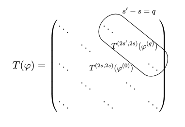
Figure 1: The operator $T(\varphi)$ whose $(2s^{\prime},2s)$ block is the Toeplitz operator of the spin $q=s^{\prime}-s$ Fourier component of an element $\varphi$ of $\Gamma(E_{reg})$.

In what follows, we replace the label of the fibers $(E^{\prime},E)$ in the Toeplitz operator with $(2s^{\prime},2s)$. For a given element $\varphi$ of $\Gamma(E_{reg})$, we define a matrix whose $(2s^{\prime},2s)$ block is given by $T^{(2s^{\prime},2s)}(\varphi^{(q)})$ with $q=s^{\prime}-s$ where $\varphi^{(q)}$ is the Fourier mode defined in (3.3) and denote it by $T(\varphi)$ (Fig. 1). If the range of $s$ and $s^{\prime}$ is not restricted, the size of $T(\varphi)$ is infinite, while that of each block $T^{(2s^{\prime},2s)}(\varphi^{(s^{\prime}-s)})$ is finite. We introduce a cut-off $\Xi$ for $s$ and $s^{\prime}$ as $|s|,|s^{\prime}|\leq\Xi$ in order to make the matrix size finite. Eventually, we take the limit in which $N\rightarrow\infty$ and $\Xi\rightarrow\infty$ with $\Xi\ll N$ kept. The blocks $T^{(2s^{\prime},2s)}(\varphi^{(s^{\prime}-s)})$ located on a line parallel to the diagonal line possess the same charge $q=s^{\prime}-s$. In this way, $T(\varphi)$ can be interpreted as a regularization of the element $\varphi$ of $\Gamma(E_{reg})$.

Then, (2.50) can be viewed as the $(2s^{\prime},2s)$ block of the commutator between $T(f\mathbbm{1})$ and $T(\varphi)$, where the $(2s,2s)$ block of $T(f\mathbbm{1})$ is given by $T^{(E,E)}(f\mathbbm{1}_{E})$ and its other off-diagonal blocks vanish.

Let us consider a regularization of the covariant derivatives. Here, we use an embedding of $M$ into $\mathbb{R}^{n}$ $(n\geq 3)$. Let $X^{A}(A=1,\dots,n)$ be embedding coordinates. The induced metric $\delta_{ab}$ on $M$ in the Lorentz frame is given by $\delta_{ab}=\partial_{a}X^{A}\partial_{b}X^{A}$ where $\partial_{a}=e^{\mu}_{a}\partial_{\mu}$. We see from (2.49) that the generalized commutator (2.50) of the Toeplitz operators corresponds to the generalized Poisson bracket (2.51) on $M$. Thus, in order to regularize the covariant derivatives as finite-size matrices, we define linear operators $\mathcal{P}_{a}$ that act on the Toeplitz operator $T(\varphi)$ as follows:

$$\mathcal{P}_{\pm}T(\varphi)=\pm i\hbar^{-1}_{N}T(\partial_{\pm}X^{A})[T(X^{A}),T(\varphi)]\mp\frac{i}{2}\hbar^{-1}_{N}[T(\partial_{\pm}X^{A}),T(X^{A})]T(\varphi)\ ,$$ (3.4)

where $\hbar_{N}=V/N$.

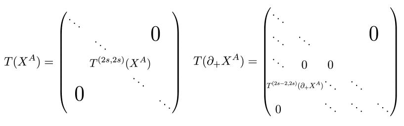
Figure 2: The structure of $T(X^{A})$ and $T(\partial_{+}X^{A})$.

(3.4) is rewritten in terms of block components as

$$\big{(}\mathcal{P}_{\pm}T(\varphi)\big{)}^{(2s^{\prime},2s)}_{mn}=\sum_{t,u}\sum_{k,l}\big{(}\mathcal{P}_{\pm}\big{)}^{(2s^{\prime},2s)(t,u)}_{(mn)(kl)}\big{(}T(\varphi)\big{)}^{(t,u)}_{kl}\ .$$ (3.5)

Here $(2s^{\prime},2s)$ and $(m,n)$ correspond to the row index, while $(t,u)$ and $(k,l)$ to the column index. In this sense, $\mathcal{P}_{\pm}$ are matrices with finite size acting on $T(\varphi)$. The non-zero blocks in $T(X^{A})$ and $T(\partial_{\pm}X^{A})$ are $(2s,2s)$ and $(2s\mp 2,2s)$, respectively (Fig. 2). In (3.5), therefore, the only block components with $2s^{\prime}-t=\mp 2$ and $2s=u$ of $\mathcal{P}_{\pm}$ are non-vanishing.

We examine the large-$N$ behavior of $\mathcal{P}_{\pm}T(\varphi)$ defined in (3.4) by using the asymptotic properties of the Toeplitz operator, (2.48) and (2.49). The first term in the RHS of (3.4) is evaluated as follows:

$$\pm i\hbar_{N}^{-1}T(\partial_{\pm}X^{A})[T(X^{A}),T(\varphi)]= T(\pm\partial_{\pm}X^{A}\epsilon^{ab}\partial_{a}X^{A}\nabla_{b}\varphi)+\mathcal{O}\quantity(\frac{1}{N})$$

$$= T(\pm\delta_{\pm a}\epsilon^{ab}\nabla_{b}\varphi)+\mathcal{O}\quantity(\frac{1}{N})$$

$$= T(i\nabla_{\pm}\varphi)+\mathcal{O}\quantity(\frac{1}{N})\ .$$ (3.6)

This is what we expected. On the other hand, the second term in the RHS of (3.4) is evaluated as

$$i\hbar_{N}^{-1}[T(\partial_{\pm}X^{A}),T(X^{A})]T(\varphi)= T(\quantity{\partial_{\pm}X^{A},X^{A}}\varphi)+\mathcal{O}\quantity(\frac{1}{N})\ .$$ (3.7)

Here we further calculate $\quantity{\partial_{\pm}X^{A},X^{A}}$:

$$\{\partial_{+}X^{A},X^{A}\}= -2i((\nabla_{+}\partial_{+}X^{A})\partial_{-}X^{A}-(\nabla_{-}\partial_{+}X^{A})\partial_{+}X^{A})$$

$$= -2i(\nabla_{+}(\partial_{+}X^{A}\partial_{-}X^{A})-\partial_{+}X^{A}\nabla_{+}\partial_{-}X^{A}-\frac{1}{2}\nabla_{-}(\partial_{+}X^{A}\partial_{+}X^{A}))$$

$$= 2i\partial_{+}X^{A}\nabla_{-}\partial_{+}X^{A}$$

$$= 0\ .$$ (3.8)

In the third equality, we used the facts that the induced metric in the local Lorentz frame is given by $\delta_{ab}=\partial_{a}X^{A}\partial_{b}X^{A}$ and that $\nabla_{+}\partial_{-}X^{A}=\nabla_{-}\partial_{+}X^{A}$. In the same way, we can show that $\{\partial_{-}X^{A},X^{A}\}=0$. Thus, the second term in the RHS of (3.4) vanishes as $\mathcal{O}(N^{-1})$ in the large-$N$ limit.

In fact, we introduce this term in order that $(\mathcal{P}_{\pm})^{\dagger}=\mathcal{P}_{\mp}$ holds for finite $N$. By using the Frobenius inner product, we define the inner product between two Toeplitz operators $T(\varphi)$ and $T(\varphi^{\prime})$ as

$$(T(\varphi),T(\varphi^{\prime}))= \mathrm{Tr}((T(\varphi))^{\dagger}T(\varphi^{\prime}))$$

$$= \sum_{s^{\prime},s}\sum_{m,n}\Big{(}\big{(}T(\varphi)\big{)}^{(s^{\prime},s)}_{mn}\Big{)}^{*}\big{(}T(\varphi^{\prime})\big{)}^{(s^{\prime},s)}_{mn}\ .$$ (3.9)

By using this inner product, we define the Hermite conjugate $(\mathcal{P}_{\pm})^{\dagger}$ of $\mathcal{P}_{\pm}$ by $((\mathcal{P}_{\pm})^{\dagger}T(\varphi),T(\varphi^{\prime}))=(T(\varphi),\mathcal{P}_{\pm}T(\varphi^{\prime}))$. Then, we see that

$$((\mathcal{P}_{+})^{\dagger}T(\varphi),T(\varphi^{\prime}))$$

$$=(T(\varphi),\mathcal{P}_{+}T(\varphi^{\prime}))$$

$$=i\hbar_{N}^{-1}\mathrm{Tr}\Big{(}(T(\varphi))^{\dagger}T(\partial_{+}X^{A})[T(X^{A}),T(\varphi^{\prime})]-\frac{1}{2}(T(\varphi))^{\dagger}[T(\partial_{+}X^{A}),T(X^{A})]T(\varphi^{\prime})\Big{)}$$

$$=i\hbar_{N}^{-1}\mathrm{Tr}\Big{(}(T(\varphi))^{\dagger}T(\partial_{+}X^{A})T(X^{A})T(\varphi^{\prime})-(T(\varphi))^{\dagger}T(\partial_{+}X^{A})T(\varphi^{\prime})T(X^{A})$$

$$\,\,\,\,\,\,\,-\frac{1}{2}(T(\varphi))^{\dagger}[T(\partial_{+}X^{A}),T(X^{A})]T(\varphi^{\prime})\Big{)}$$

$$=i\hbar_{N}^{-1}\mathrm{Tr}\Big{(}(T(\varphi))^{\dagger}T(X^{A})T(\partial_{+}X^{A})T(\varphi^{\prime})-T(X^{A})(T(\varphi))^{\dagger}T(\partial_{+}X^{A})T(\varphi^{\prime})$$

$$\,\,\,\,\,\,\,+\frac{1}{2}(T(\varphi))^{\dagger}[T(\partial_{+}X^{A}),T(X^{A})]T(\varphi^{\prime})\Big{)}$$

$$=i\hbar_{N}^{-1}\mathrm{Tr}\Big{(}[(T(\varphi))^{\dagger},T(X^{A})]T(\partial_{+}X^{A})T(\varphi^{\prime})+\frac{1}{2}(T(\varphi))^{\dagger}[T(\partial_{+}X^{A}),T(X^{A})]T(\varphi^{\prime})\Big{)}$$

$$=\mathrm{Tr}\bigg{(}\Big{(}-i\hbar_{N}^{-1}T(\partial_{-}X^{A})[T(X^{A}),T(\varphi)]\Big{)}^{\dagger}T(\varphi^{\prime})+\Big{(}\frac{i}{2}\hbar_{N}^{-1}[T(\partial_{-}X^{A}),T(X^{A})]T(\varphi)\Big{)}^{\dagger}T(\varphi^{\prime})\bigg{)}$$

$$=(\mathcal{P}_{-}T(\varphi),T(\varphi^{\prime}))\ .$$ (3.10)

In the third equality, we expanded the commutator in the first term. In the forth equality, we exchanged $T(\partial_{+}X^{A})$ and $T(X^{A})$ in the first term, changed the sign of the third term and used the cyclic property of the trace in the second term. In the fifth equality, we put the first and second terms together in the commutator. Thus, we see that $(\mathcal{P}_{+})^{\dagger}=\mathcal{P}_{-}$ for finite $N$. Similarly, we see that $(\mathcal{P}_{-})^{\dagger}=\mathcal{P}_{+}$.

In this way, $\mathcal{P}_{\pm}$ defined in (3.4) are finite-size matrices that serves as a regularization of the covariant derivatives. Note that $\mathcal{P}_{\pm}$ is local Lorentz invariant. The Toeplitz operators are defined as (2.43) with a inner product that is local Lorentz invariant. Then, the U(1) charges of $X^{A}$ and $\partial_{\pm}X^{A}$ are conserved. Thus, the index $\pm$ of $\mathcal{P}_{\pm}$ is not transformed under the local Lorentz transformation. This implies that the index of $\mathcal{P}_{\pm}$ is equivalent to that of the covariant derivative $\nabla_{(a)}$ acting on $\Gamma(E_{reg})$. To summarize, $\mathcal{P}_{a}$ are finite-size matrices corresponding to $i\nabla_{(a)}$.

By using the commutator between $\mathcal{P}_{+}$ and $\mathcal{P}_{-}$, we also define $\mathcal{P}_{3}$:

$$\mathcal{P}_{3}T(\varphi)= [\mathcal{P}_{+},\mathcal{P}_{-}]T(\varphi)$$

$$= \mathcal{P}_{+}(\mathcal{P}_{-}T(\varphi))-\mathcal{P}_{-}(\mathcal{P}_{+}T(\varphi))\ .$$ (3.11)

Because the second term of (3.4) is $\mathcal{O}(N^{-1})$, we ignore this term below. The first term in the RHS of (3.11) is evaluated as

$$\mathcal{P}_{+}(\mathcal{P}_{-}T(\varphi))= -\mathcal{P}_{+}(i\hbar_{N}^{-1}T(\partial_{-}X^{A})[T(X^{A}),T(\varphi)])+\mathcal{O}\quantity(\frac{1}{N})$$

$$= \hbar_{N}^{-2}T(\partial_{+}X^{B})[T(X^{B}),T(\partial_{-}X^{A})[T(X^{A}),T(\varphi)]]+\mathcal{O}\quantity(\frac{1}{N})$$

$$= \hbar_{N}^{-2}T(\partial_{+}X^{B})T(\partial_{-}X^{A})[T(x^{B}),[T(X^{A}),T(\varphi)]]$$

$$+\hbar_{N}^{-2}T(\partial_{+}X^{B})[T(X^{B}),T(\partial_{-}X^{A})][T(X^{A}),T(\varphi)]+\mathcal{O}\quantity(\frac{1}{N})\ .$$ (3.12)

Similarly, the second term in the RHS of (3.11) is evaluated. Then, $\mathcal{P}_{3}$ is evaluated as

$$\mathcal{P}_{3}T(\varphi)= \hbar_{N}^{-2}\Big{(}T(\partial_{+}X^{B})T(\partial_{-}X^{A})[T(X^{B}),[T(X^{A}),T(\varphi)]]$$

$$+T(\partial_{+}X^{B})[T(X^{B}),T(\partial_{-}X^{A})][T(X^{A}),T(\varphi)]$$

$$-T(\partial_{-}X^{A})T(\partial_{+}X^{B})[T(X^{A}),[T(X^{B}),T(\varphi)]]$$

$$-T(\partial_{-}X^{A})[T(X^{A}),T(\partial_{+}X^{B})][T(X^{B}),T(\varphi)]\Big{)}+\mathcal{O}\quantity(\frac{1}{N})$$

$$= \hbar_{N}^{-2}\Big{(}T(\partial_{+}X^{B})T(\partial_{-}X^{A})[T(X^{B}),[T(X^{A}),T(\varphi)]]$$

$$+T(\partial_{+}X^{B})[T(X^{B}),T(\partial_{-}X^{A})][T(X^{A}),T(\varphi)]$$

$$-T(\partial_{+}X^{B})T(\partial_{-}X^{A})[T(X^{A}),[T(X^{B}),T(\varphi)]]$$

$$-T(\partial_{-}X^{A})[T(X^{A}),T(\partial_{+}X^{B})][T(X^{B}),T(\varphi)]\Big{)}+\mathcal{O}\quantity(\frac{1}{N})$$

$$= \hbar_{N}^{-2}\Big{(}T(\partial_{+}X^{B})T(\partial_{-}X^{A})[[T(X^{A}),T(X^{B})],T(\varphi)]$$

$$+T(\partial_{+}X^{B})[T(X^{B}),T(\partial_{-}X^{A})][T(X^{A}),T(\varphi)]$$

$$-T(\partial_{-}X^{A})[T(X^{A}),T(\partial_{+}X^{B})][T(X^{B}),T(\varphi)]\Big{)}+\mathcal{O}\quantity(\frac{1}{N})\ .$$ (3.13)

In the second equality, using (2.48), we exchanged $T(\partial_{-}X^{A})$ and $T(\partial_{+}X^{B})$ in the third term. In the third equality, we used the Jacobi identity for the first and third terms. Furthermore, using (2.48), (2.49) and (3.6), we can evaluate the second term in the most right-hand side of (3.13) as

$$\hbar_{N}^{-2}T(\partial_{+}X^{B})[T(X^{B}),T(\partial_{-}X^{A})][T(X^{A}),T(\varphi)]$$

$$=\hbar_{N}^{-1}T(\nabla_{+}\partial_{-}X^{A})T(\{X^{A},\varphi\})+\mathcal{O}\quantity(\frac{1}{N})$$

$$=\hbar_{N}^{-1}T(\nabla_{+}\partial_{-}X^{A}\{X^{A},\varphi\})+\mathcal{O}\quantity(\frac{1}{N})\ .$$ (3.14)

Finally, we calculate $\nabla_{+}\partial_{-}X^{A}\{X^{A},\varphi\}$ as follows:

$$\nabla_{+}\partial_{-}X^{A}\{X^{A},\varphi\}= -2i\nabla_{+}\partial_{-}X^{A}(\partial_{+}X^{A}\nabla_{-}\varphi-\partial_{-}X^{A}\nabla_{+}\varphi)$$

$$= -2i\{(\nabla_{-}\partial_{+}X^{A})\partial_{+}X^{A}\nabla_{-}\varphi-(\nabla_{+}\partial_{-}X^{A})\partial_{-}X^{A}\nabla_{+}\varphi\}$$

$$= -i\{\nabla_{-}(\delta_{++})\nabla_{-}\varphi-\nabla_{+}(\delta_{--})\nabla_{+}\varphi\}$$

$$= 0\ .$$ (3.15)

Hence, the second term in the most right-hand side of (3.13) behaves as $\mathcal{O}(N^{-1})$. Similarly, we can also evaluate the third term in the RHS of (3.13). Thus, $\mathcal{P}_{3}$ behaves as

$$\mathcal{P}_{3}T(\varphi)=\hbar_{N}^{-2}T(\partial_{+}X^{A})T(\partial_{-}X^{B})[[T(X^{A}),T(X^{B})],T(\varphi)]+\mathcal{O}\quantity(\frac{1}{N})\ .$$ (3.16)

3.2 Example: $S^{2}$

As in section 2.2, we consider a unit sphere $S^{2}$ embedded in $\mathbb{R}^{3}$ and apply to it the formulation developed in the previous subsection. In particular, we see that $\mathcal{P}_{a}$ defined in the previous subsection form the su(2) Lie algebra as seen in section 2.2.

Let $X^{A}$ be again embedding coordinates of $S^{2}$ and $(z,\bar{z})$ be the stereographic projection of $S^{2}$ from the north pole to the $X^{1}-X^{2}$ plane:

$$X^{1}=\frac{z+\bar{z}}{1+|z|^{2}}\ ,\;X^{2}=-i\frac{z-\bar{z}}{1+|z|^{2}}\ ,\;X^{3}=\frac{1-|z|^{2}}{1+|z|^{2}}\ .$$ (3.17)

The induced metric, the zweibein, the inverse of the zweibein and the spin connection are given by

$$g_{z\bar{z}}=g_{\bar{z}z}=\frac{2}{(1+|z|^{2})^{2}}\ ,\;\;g_{zz}=g_{\bar{z}\bar{z}}=0\ ,$$

$$e^{1}=\frac{dz+d\bar{z}}{1+|z|^{2}}\ ,\;\;e^{2}=-i\frac{dz-d\bar{z}}{1+|z|^{2}}\ ,$$

$$e_{1}=\frac{1}{2}(1+|z|^{2})(\partial_{z}+\partial_{\bar{z}})\ ,\;\;e_{2}=\frac{i}{2}(1+|z|^{2})(\partial_{z}-\partial_{\bar{z}})\ ,$$

$$\Omega^{1}{}_{2}=-i\frac{\bar{z}dz-zd\bar{z}}{1+|z|^{2}}\ ,$$ (3.18)

as in section 2.2. The volume form is given by

$$\omega= i\sqrt{\det g}dz\wedge d\bar{z}$$

$$= i\frac{2}{(1+|z|^{2})^{2}}dz\wedge d\bar{z}\ ,$$ (3.19)

and the volume is given by

$$V=\frac{1}{2\pi}\int_{S^{2}}\omega=2\ .$$ (3.20)

Next, as a connection 1-form in the complex line bundle $L$, we adopt the Wu-Yang monopole,

$$A=-\frac{i}{2}\frac{\bar{z}dz-zd\bar{z}}{1+|z|^{2}}\ ,$$ (3.21)

which satisfies that $F=dA=\omega/V$. Note that $A=\frac{1}{2}\Omega^{1}{}_{2}$. The connections in the fiber bundles $E$ and $E^{\prime}$ are given by

$$A^{(E)}= s\Omega^{1}{}_{2}\ ,$$

$$A^{(E^{\prime})}= s^{\prime}\Omega^{1}{}_{2}\ ,$$ (3.22)

respectively. The Dirac operator $D^{(E)}$ on $\Gamma(S\otimes L^{\otimes N}\otimes E)$ reads

$$D^{(E)}= \begin{pmatrix}0&D^{(E)}_{-}\\ D^{(E)}_{+}&0\end{pmatrix}$$ (3.23)

with

$$D_{-}^{(E)}= i\quantity{(1+|z|^{2})\partial_{z}-\frac{N+2s+1}{2}\bar{z}}\ ,$$

$$D_{+}^{(E)}= i\quantity{(1+|z|^{2})\partial_{\bar{z}}+\frac{N+2s-1}{2}\bar{z}}\ .$$ (3.24)

For $N\geq 2s+1$, $D^{(E)}_{-}$ has no normalizable zero modes so that $\mathrm{Ker}D^{(E)}_{-}$ is empty. In what follows, we assume that this condition is satisfied. Then, the orthonormalized zero modes take the following form:

$$\psi^{(E)}_{n}=\begin{pmatrix}\psi^{(E)+}_{n}\\ 0\end{pmatrix},$$ (3.25)

$$\psi^{(E)+}_{n}=\sqrt{\frac{N+2s}{4\pi}}\binom{N+2s-1}{n}^{\frac{1}{2}}\frac{z^{n}}{(1+|z|^{2})^{\frac{N+2s-1}{2}}}\ ,$$ (3.26)

where $n=0,1,\dots,N+2s-1$. By using the formula,

$$\frac{1}{2\pi}\int idzd\bar{z}\frac{z^{a}\bar{z}^{b}}{(1+|z|^{2})^{c}}=\delta_{ab}\frac{\Gamma(a+1)\Gamma(c-a-1)}{\Gamma(c)}\ ,$$ (3.27)

where $\Gamma(a)$ is the Gamma function, we can calculate the Toeplitz operators of $X^{A}$. The result is

$$\big{(}T(X^{+})\big{)}^{(2s,2s)}_{mn} =\delta_{m-1,n}\frac{2}{N+2s+1}\sqrt{m(N+2s-m)}\ ,$$

$$\big{(}T(X^{-})\big{)}^{(2s,2s)}_{mn} =\Big{(}\big{(}T(X^{+})\big{)}^{(s,s)}_{mn}\Big{)}^{\dagger}$$

$$=\delta_{m+1,n}\frac{2}{N+2s+1}\sqrt{(m+1)(N+2s-m-1)}\ ,$$

$$\big{(}T(X^{3})\big{)}^{(2s,2s)}_{mn} =\delta_{m,n}\frac{N+2s-2n-1}{N+2s+1}\ ,$$ (3.28)

where $m,\ n=0,\ldots,N+2s-1$. These operators satisfy the su(2) Lie algebra:

$$[T(X^{A}),T(X^{B})]^{(2s,2s)}=-\frac{2}{N+2s+1}i\epsilon^{ABC}\big{(}T(X^{C})\big{)}^{(2s,2s)}\ .$$ (3.29)

Furthermore, noting that $\partial_{\pm}X^{A}$ possess the charge $Q=\mp\frac{1}{2}$, we can calculate the Toeplitz operators of $\partial_{\pm}X^{A}$ as

$$\big{(}T(\partial_{+}X^{+})\big{)}^{(2s-2,2s)}_{m^{\prime}n}=\delta_{m^{\prime},n}\sqrt{\frac{(N+2s-n-1)(N+2s-n-2)}{(N+2s)(N+2s-1)}}\ ,$$

$$\big{(}T(\partial_{+}X^{-})\big{)}^{(2s-2,2s)}_{m^{\prime}n}=-\delta_{m^{\prime}+2,n}\sqrt{\frac{n(n-1)}{(N+2s)(N+2s-1)}}\ ,$$

$$\big{(}T(\partial_{+}X^{3})\big{)}^{(2s-2,2s)}_{m^{\prime}n}=-\delta_{m^{\prime}+1,n}\sqrt{\frac{n(N+2s-n-1)}{(N+2s)(N+2s-1)}}\ ,$$

$$\big{(}T(\partial_{-}X^{+})\big{)}^{(2s+2,2s)}_{m^{\prime\prime}n}=-\delta_{m^{\prime\prime},n+2}\sqrt{\frac{m^{\prime\prime}(m^{\prime\prime}-1)}{(N+2s+2)(N+2s+1)}}\ ,$$

$$\big{(}T(\partial_{-}X^{-})\big{)}^{(2s+2,2s)}_{m^{\prime\prime}n}=\delta_{m^{\prime\prime},n}\sqrt{\frac{(N+2s-m^{\prime\prime}+1)(N+2s-m^{\prime\prime})}{(N+2s+2)(N+2s+1)}}\ ,$$

$$\big{(}T(\partial_{-}X^{3})\big{)}^{(2s+2,2s)}_{m^{\prime\prime}n}=-\delta_{m^{\prime\prime},n+1}\sqrt{\frac{m^{\prime\prime}(N+2s-m^{\prime\prime}+1)}{(N+2s+2)(N+2s+1)}}\ ,$$ (3.30)

where $m^{\prime}=0,\ldots,N+2s-3$, $m^{\prime\prime}=0,\ldots,N+2s+1$ and $n=0,\ldots,N+2s-1$.

By using (3.28) and (3.30), we can calculate $\mathcal{P}_{\pm}$ and $\mathcal{P}_{3}$ that we defined in the previous subsection. In appendix B, we present concrete forms of $\mathcal{P}_{\pm}$. In appendix A, we evaluate $\mathcal{P}_{3}$ by using (3.16). It is given up to $\mathcal{O}(N^{-1})$ by

$$\big{(}\mathcal{P}_{3}T(\varphi)\big{)}^{(2s^{\prime},2s)}_{mn}=-\frac{s^{\prime}-s}{2}\big{(}T(\varphi)\big{)}^{(2s^{\prime},2s)}_{mn}\ .$$ (3.31)

As anticipated from (2.35) and (3.16), $\mathcal{P}_{3}$ is proportional to the charge of fields. Indeed, the charges are the eigenvalues of the local Lorentz generator $O_{+-}$.

We also see from this that the action of the commutators between $\mathcal{P}_{3}$ and $\mathcal{P}_{\pm}$ on the Toeplitz operator are given up to $\mathcal{O}(N^{-1})$ as

$$\big{(}[\mathcal{P}_{3},\mathcal{P}_{+}]T(\varphi)\big{)}^{(2s^{\prime}-2,2s)}= \frac{1}{2}\big{(}\mathcal{P}_{+}T(\varphi)\big{)}^{(2s^{\prime}-2,2s)}\ ,$$

$$\big{(}[\mathcal{P}_{3},\mathcal{P}_{-}]T(\varphi)\big{)}^{(2s^{\prime}+2,2s)}= -\frac{1}{2}\big{(}\mathcal{P}_{-}T(\varphi)\big{)}^{(2s^{\prime}+2,2s)}\ .$$ (3.32)

Thus, the commutators between $\mathcal{P}_{\pm}$ and $\mathcal{P}_{3}$ are summarized up to $\mathcal{O}(N^{-1})$ as

$$[\mathcal{P}_{+},\mathcal{P}_{-}]=\mathcal{P}_{3}\ ,$$ (3.33)

$$[\mathcal{P}_{3},\mathcal{P}_{\pm}]=\pm\frac{1}{2}\mathcal{P}_{\pm}\ ,$$ (3.34)

which are the su(2) Lie algebra. This reproduces (2.35) and (2.36) in section 2.2.

3.3 Example: $T^{2}$

In this subsection, we consider a torus $T^{2}$ embedded in $\mathbb{R}^{4}$. See [32] for the detailed derivation of the Dirac zero modes and the Toeplitz operators. As the orthonormal coordinates $(x^{1},x^{2})$ of $T^{2}$ satisfy the periodicity $x^{a}\sim x^{a}+2\pi$, we introduce the fundamental functions $u$ and $v$ on $T^{2}$ as

$$u(x^{1},x^{2})=e^{ix^{1}},\quad v(x^{1},x^{2})=e^{ix^{2}}.$$ (3.35)

Then, the isometric embedding $X^{A}$ of $T^{2}$ in $\mathbb{R}^{4}$ is defined by

$$X^{1}(x^{1},x^{2})=\cos{x^{1}}=\frac{1}{2}(u+u^{*})\ ,\;\;X^{2}(x^{1},x^{2})=\sin{x^{1}}=\frac{1}{2i}(u-u^{*})\ ,$$

$$X^{3}(x^{1},x^{2})=\cos{x^{2}}=\frac{1}{2}(v+v^{*})\ ,\;\;X^{4}(x^{1},x^{2})=\sin{x^{2}}=\frac{1}{2i}(v-v^{*})\ .$$ (3.36)

The derivatives of those satisfy

$$\partial_{1}X^{1}=-X^{2}\ ,\;\;\partial_{1}X^{2}=X^{1}\ ,$$

$$\partial_{2}X^{3}=-X^{4}\ ,\;\;\partial_{2}X^{4}=X^{3}\ ,$$

$$\partial_{2}X^{1}=\partial_{2}X^{2}=\partial_{1}X^{3}=\partial_{1}X^{4}=0\ .$$ (3.37)

The spin connection of $T^{2}$ is zero. The volume form is given by

$$\omega=dx^{1}\wedge dx^{2}\ .$$ (3.38)

The volume of $T^{2}$ is given by

$$V=\frac{1}{2\pi}\int_{T^{2}}\omega=\int_{T^{2}}dx^{1}dx^{2}=2\pi\ ,$$ (3.39)

and $\hbar_{N}=2\pi/N$. We adopt the following U(1) connection $A$ of the line bundle $L$ as

$$A=\frac{1}{4\pi}(-x^{2}dx^{1}+x^{1}dx^{2})\ .$$ (3.40)

This satisfies $F=dA=\omega/V$. $A$ varies under the shift $x^{a}\to x^{a}+2\pi$ as

$$A(x^{1}+2\pi,x^{2})=A(x^{1},x^{2})+\frac{1}{2}dx^{2}\ ,$$

$$A(x^{1},x^{2}+2\pi)=A(x^{1},x^{2})-\frac{1}{2}dx^{1}\ .$$ (3.41)

This is considered as a gauge transformation. Then, the spinor field $\psi\in\Gamma(S\otimes L^{\otimes N})$ satisfies the boundary condition,

$$\psi(x^{1}+2\pi,x^{2})=\exp\quantity(i\frac{N}{2}x^{2})\psi(x^{1},x^{2})\ ,$$

$$\psi(x^{1},x^{2}+2\pi)=\exp\quantity(-i\frac{N}{2}x^{1})\psi(x^{1},x^{2})\ .$$ (3.42)

The Dirac operator $D^{(E)}$ on $\Gamma(S\otimes L^{\otimes N}\otimes E)$ reads

$$D^{(E)}= \begin{pmatrix}0&D^{(E)}_{-}\\ D^{(E)}_{+}&0\end{pmatrix}$$ (3.43)

with

$$D_{-}^{(E)}= i(\partial_{1}-i\partial_{2}-\frac{N}{4\pi}(x^{1}-ix^{2}))\ ,$$

$$D_{+}^{(E)}= i(\partial_{1}+i\partial_{2}+\frac{N}{4\pi}(x^{1}+ix^{2}))\ .$$ (3.44)

As in the case of $S^{2}$, for sufficiently large $N$, $D^{(E)}_{-}$ has no normalizable zero modes so that $\mathrm{Ker}D^{(E)}_{-}$ is empty. Then, the orthonormalized zero modes of $D^{(E)}$ are given as follows:

$$\psi^{(E)}_{n}=\begin{pmatrix}\psi^{(E)+}_{n}\\ 0\end{pmatrix},$$ (3.45)

$$\psi^{(E)+}_{n}=d_{n}e^{-\frac{N}{4\pi}(x^{2})^{2}}e^{i\frac{N}{4\pi}x^{1}x^{2}}\sum_{k\in\mathbb{Z}}e^{-\pi(Nk^{2}+2nk)}e^{i(Nk+n)(x^{1}+ix^{2})}\ ,$$ (3.46)

where $n=1,\dots,N$. The normalization factor $d_{n}$ is given by

$$d_{n}=\quantity(\frac{N}{8\pi^{4}})^{1/4}e^{-\frac{\pi}{N}n^{2}}\ .$$ (3.47)

Note that the Dirac zero modes are independent of the charge of $E$. When we perform the Berezin-Toeplitz quantization, we must be careful about the charge of the component of the tensor field. For example, the embedding coordinate $X^{1}$ and the derivatives $2\partial_{\pm}X^{2}$ are the same function of $x^{a}$, but they have the charges $0$ and $\mp 1$, respectively. Therefore, the non-zero blocks of the Toeplitz operators $T(X^{1})$ and $T(\partial_{\pm}X^{2})$ are $(2s,2s)$ and $(2s\mp 2,2s)$ blocks, respectively, and all these blocks are the same matrices.

Now, let us compute the Toplitz operators. Suppose that $u$ and $v$ have the charge $s^{\prime}-s$. Then, the Toeplitz operators $\big{(}T(u)\big{)}^{(2s^{\prime},2s)}$ and $\big{(}T(v)\big{)}^{(2s^{\prime},2s)}$ are given by the clock-shift matrices $U$ and $V$ that take the following forms

$$U=e^{-\frac{\pi}{2N}}\begin{pmatrix}&&&&1\\ 1&&&&\\ &1&&&\\ &&\ddots&&\\ &&&1&\end{pmatrix}\ ,\;\;V=e^{-\frac{\pi}{2N}}\begin{pmatrix}q^{-1}&&&\\ &q^{-2}&&\\ &&\ddots&\\ &&&q^{-N}\end{pmatrix}$$ (3.48)

with $q=e^{i2\pi/N}$. These matrices satisfy the ’t Hooft-Weyl algebra,

$$UV=qVU\ .$$ (3.49)

Hence, the non-zero components of the Toplitz operators of the embedding coordinates $X^{A}$ are given by

$$\big{(}T(X^{1})\big{)}^{(2s,2s)}=\frac{1}{2}(U+U^{\dagger})\ ,\;\;\big{(}T(X^{2})\big{)}^{(2s,2s)}=\frac{1}{2i}(U-U^{\dagger})\ ,$$

$$\big{(}T(X^{3})\big{)}^{(2s,2s)}=\frac{1}{2}(V+V^{\dagger})\ ,\;\;\big{(}T(X^{4})\big{)}^{(2s,2s)}=\frac{1}{2i}(V-V^{\dagger})\ ,$$ (3.50)

and those of the derivatives $\partial_{a}X^{A}$ are given by

$$\big{(}T(\partial_{+}X^{1})\big{)}^{(2s-2,2s)}=\big{(}T(\partial_{-}X^{1})\big{)}^{(2s+2,2s)}=-\frac{1}{4i}(U-U^{\dagger})\ ,$$

$$\big{(}T(\partial_{+}X^{2})\big{)}^{(2s-2,2s)}=\big{(}T(\partial_{-}X^{2})\big{)}^{(2s-2,2s)}=\frac{1}{4}(U+U^{\dagger})\ ,$$

$$\big{(}T(\partial_{+}X^{3})\big{)}^{(2s-2,2s)}=-\big{(}T(\partial_{-}X^{3})\big{)}^{(2s+2,2s)}=\frac{1}{4}(V-V^{\dagger})\ ,$$

$$\big{(}T(\partial_{+}X^{4})\big{)}^{(2s-2,2s)}=-\big{(}T(\partial_{-}X^{4})\big{)}^{(2s-2,2s)}=-\frac{i}{4}(V+V^{\dagger})\ .$$ (3.51)

Substituting these into (3.4), we obtain the non-zero blocks of $\mathcal{P}_{\pm}$ as

$$(\mathcal{P}_{+})^{(2s^{\prime}-2,2s)(2s^{\prime},2s)}_{(mn)(kl)}=-i\hbar_{N}^{-1}\big{(}T(\partial_{+}X^{A})\big{)}^{(2s^{\prime}-2,2s^{\prime})}_{mk}\big{(}T(X^{A})\big{)}^{(2s,2s)}_{ln}\ ,$$

$$(\mathcal{P}_{-})^{(2s^{\prime}+2,2s)(2s^{\prime},2s)}_{(mn)(kl)}=i\hbar_{N}^{-1}\big{(}T(\partial_{-}X^{A})\big{)}^{(2s^{\prime}+2,2s^{\prime})}_{mk}\big{(}T(X^{A})\big{)}^{(2s,2s)}_{ln}\ ,$$ (3.52)

where we used

$$T(\partial_{\pm}X^{A})T(X^{A})=0\ .$$ (3.53)

Note that the size of $\big{(}\mathcal{P}_{\pm}\big{)}^{(2s^{\prime}\mp 2,2s)(2s^{\prime},2s)}$ on $T^{2}$ is independent of the charges $s$ and $s^{\prime}$ unlike that on $S^{2}$. Then, as shown in the appendix A, $\mathcal{P}_{3}T(\varphi)$ behaves as

$$\mathcal{P}_{3}T(\varphi)=\mathcal{O}\quantity(\frac{1}{N})$$ (3.54)

for sufficiently large $N$. This reflects the flatness of $T^{2}$.

4 Conclusion and discussion

In this paper, we studied regularization of matrices in the covariant derivatives interpretation of matrix models. By using the Berezin-Toeplitz quantization, we represented the covariant derivatives in two dimensions in the covariant derivative interpretation as matrices with finite size. We verified that the constructed matrices in the case of $S^{2}$ and $T^{2}$ indeed satisfy the properties seen in the covariant derivative interpretation.

In regularizing the covariant derivatives, we introduced the embedding coordinates $X^{A}$ $A=1,\ldots,n$ with $n\geq 3$. Choosing $X^{A}$ is likely to specify a way of regularization. It is expected that physical quantities are independent of the choice of $X^{A}$ in the large-$N$ limit. We leave verification of this as a future work. Note that as in the covariant derivative interpretation two-dimensional curved spacetimes are represented by only the two matrices $\mathcal{P}_{\pm}$ although it is needed to embed them into $\mathbb{R}^{n}$ $(n\geq 3)$. On the other hand, for instance, the fuzzy sphere is represented by three matrices. In this sense, our formulation is different from the representation of fuzzy manifolds in terms of matrices with finite size.

In [34], the matrices $T(X^{A})$ in Fig. 2 and the limit in which $N\rightarrow\infty$ and $\Xi\rightarrow\infty$ with $\Xi\ll N$ kept are used to obtain planar $\mathcal{N}=4$ super Yang-Mills theory on $\mathbb{R}\times S^{3}$ from the plane wave matrix model [4] as a generalization of the large-$N$ reduction [35] to curved spaces. The latter is obtained by dimensional reducing the former to one dimension. In that case, $S^{3}$ is constructed from the three matrices $T(X^{A})$, while it is constructed from $\mathcal{P}_{\pm}$ and $\mathcal{P}_{3}$ in our formulation. However, the commutators between $T(X^{A})$ and $T(\varphi)$ do not give the action of $O_{+-}$ on $T(\varphi)$ unlike the action of $\mathcal{P}_{3}$ on $T(\varphi)$. This difference comes from the existence of $T(\partial_{\pm}X^{A})$ in the first term of the RHS of (3.4).

Some future directions are in order. First, we need to generalize the construction in this paper to higher dimensional cases. It is interesting to perform perturbative calculation of physical quantities using matrices with finite size in the covariant derivative interpretation. Finally, we would like to derive geometries from the results in the numerical simulations of the type IIB matrix model by using the formulation developed in this paper.

Appendix A Evaluation of $\mathcal{P}_{3}$ on $S^{2}$ and $T^{2}$

In this appendix, we evaluate $\mathcal{P}_{3}$ on $S^{2}$ and $T^{2}$. First, we show that $\mathcal{P}_{3}$ is given on $S^{2}$ as (3.31). By using (3.29), we calculate (3.16) as follows:

$$\big{(}\mathcal{P}_{3}T(\varphi)\big{)}^{(2s^{\prime},2s)}$$

$$=\hbar_{N}^{-2}\big{(}T(\partial_{+}X^{A})\big{)}^{(2s^{\prime},2s^{\prime}+2)}\big{(}T(\partial_{-}X^{B})\big{)}^{(2s^{\prime}+2,2s^{\prime})}[[T(X^{A}),T(X^{B})],T(\varphi)]^{(2s^{\prime},2s)}+\mathcal{O}\quantity(\frac{1}{N})$$

$$=-2i\hbar_{N}^{-2}\epsilon^{ABC}\big{(}T(\partial_{+}X^{A})\big{)}^{(2s^{\prime},2s^{\prime}+2)}\big{(}T(\partial_{-}X^{B})\big{)}^{(2s^{\prime}+2,2s^{\prime})}$$

$$\quad\times\bigg{(}\frac{1}{N+2s^{\prime}+1}\big{(}T(X^{C})\big{)}^{(2s^{\prime},2s^{\prime})}\big{(}T(\varphi)\big{)}^{(2s^{\prime},2s)}-\frac{1}{N+2s+1}\big{(}T(\varphi)\big{)}^{(2s^{\prime},2s)}\big{(}T(X^{C})\big{)}^{(2s,2s)}\bigg{)}$$

$$\quad+\mathcal{O}\quantity(\frac{1}{N})$$

$$=\frac{4i(s^{\prime}-s)}{(N+2s^{\prime}+1)(N+2s+1)}\hbar_{N}^{-2}\epsilon^{ABC}\big{(}T(\partial_{+}X^{A})\big{)}^{(2s^{\prime},2s^{\prime}+2)}\big{(}T(\partial_{-}X^{B})\big{)}^{(2s^{\prime}+2,2s^{\prime})}$$

$$\quad\times\big{(}T(X^{C})\big{)}^{(2s^{\prime},2s^{\prime})}\big{(}T(\varphi)\big{)}^{(2s^{\prime},2s)}$$

$$\quad-\frac{2i}{N+2s+1}\hbar_{N}^{-2}\epsilon^{ABC}\big{(}T(\partial_{+}X^{A})\big{)}^{(2s^{\prime},2s^{\prime}+2)}\big{(}T(\partial_{-}X^{B})\big{)}^{(2s^{\prime}+2,2s^{\prime})}[T(X^{C}),T(\varphi)]^{(2s^{\prime},2s)}$$

$$\quad+\mathcal{O}\quantity(\frac{1}{N})\ .$$ (A.1)

We recall that $s$ and $s^{\prime}$ satisfy $|s|,|s^{\prime}|\ll N$. By using the asymptotic properties of the Toeplitz operator, (2.48) and (2.49), we can evaluate the second term in the most right-hand side of (A.1) as

$$-\frac{2i}{N+2s+1}\hbar_{N}^{-2}\epsilon^{ABC}\big{(}T(\partial_{+}X^{A})\big{)}^{(2s^{\prime},2s^{\prime}+2)}\big{(}T(\partial_{-}X^{B})\big{)}^{(2s^{\prime}+2,2s^{\prime})}[T(X^{C}),T(\varphi)]^{(2s^{\prime},2s)}$$

$$=\frac{N}{N+2s+1}\big{(}T(\epsilon^{ABC}\partial_{+}X^{A}\partial_{-}X^{B}\{X^{C},\varphi\})\big{)}^{(2s^{\prime},2s)}+\mathcal{O}\quantity(\frac{1}{N})\ .$$ (A.2)

Furthermore, noting that the embedding coordinates $X^{A}$ of $S^{2}$ satisfy that $\{X^{A},X^{B}\}=\epsilon^{ABC}X^{C}$, we obtain

$$\epsilon^{ABC}\partial_{+}X^{A}\partial_{-}X^{B}\{X^{C},\varphi\} =\frac{i}{4}\epsilon^{ABC}\{X^{A},X^{B}\}\{X^{C},\varphi\}$$

$$=\frac{i}{4}\epsilon^{ABC}\epsilon^{ABD}X^{D}\{X^{C},\varphi\}$$

$$=X^{C}(\partial_{+}X^{C}\partial_{-}\varphi-\partial_{-}X^{C}\partial_{+}\varphi)$$

$$=\frac{1}{2}(\partial_{+}(X^{C}X^{C})\partial_{-}\varphi-\partial_{-}(X^{C}X^{C})\partial_{+}\varphi)=0\ .$$ (A.3)

Hence, (A.1) leads to

$$\big{(}\mathcal{P}_{3}T(\varphi)\big{)}^{(2s^{\prime},2s)}$$

$$=\frac{i(s^{\prime}-s)N^{2}}{(N+2s^{\prime}+1)(N+2s+1)}\epsilon^{ABC}\big{(}T(\partial_{+}X^{A})\big{)}^{(2s^{\prime},2s^{\prime}+2)}\big{(}T(\partial_{-}X^{B})\big{)}^{(2s^{\prime}+2,2s^{\prime})}$$

$$\times\big{(}T(X^{C})\big{)}^{(2s^{\prime},2s^{\prime})}\big{(}T(\varphi)\big{)}^{(2s^{\prime},2s)}+\mathcal{O}\quantity(\frac{1}{N})\ .$$ (A.4)

Finally, substituting the concrete forms of the Toeplitz operators on $S^{2}$, (3.28) and (3.30), into (A.4) yields

$$\big{(}\mathcal{P}_{3}T(\varphi)\big{)}^{(2s^{\prime},2s)} =-\frac{s^{\prime}-s}{2}\frac{N^{2}(N+2s^{\prime}-1)}{(N+2s+1)(N+2s^{\prime}+1)^{2}}\big{(}T(\varphi)\big{)}^{(2s^{\prime},2s)}+\mathcal{O}\quantity(\frac{1}{N})$$

$$=-\frac{s^{\prime}-s}{2}\big{(}T(\varphi)\big{)}^{(2s^{\prime},2s)}+\mathcal{O}\quantity(\frac{1}{N})\ .$$ (A.5)

The above result can also be obtained by using the asymptotic expansion (2.44). From (2.45)-(2.47), $[T(X^{A}),T(X^{B})]^{(2s,2s)}$ is evaluated as

$$[T(X^{A}),T(X^{B})]^{(2s,2s)}$$

$$=\hbar_{N}\big{(}T(\{X^{A},X^{B}\})\big{)}^{(2s,2s)}+\hbar_{N}^{2}\big{(}T(\widetilde{C}_{2}(X^{A},X^{B}))\big{)}^{(2s,2s)}+\hbar_{N}^{2}\bigg{(}T\Big{(}iF^{(E)}_{12}\{X^{A},X^{B}\}\Big{)}\bigg{)}^{(2s,2s)}$$

$$\quad+\mathcal{O}\quantity(\frac{1}{N^{3}})\ ,$$ (A.6)

where $\widetilde{C}_{2}(X^{A},X^{B})$ is defined as

$$\widetilde{C}_{2}(X^{A},X^{B}) =C_{2}(X^{A},X^{B})-C_{2}(X^{B},X^{A})-iF^{(E)}_{12}\{X^{A},X^{B}\}$$

$$=\frac{i}{4}\quantity(R\{X^{A},X^{B}\}+(g^{ab}W^{cd}+W^{ab}g^{cd})(\nabla_{a}\partial_{c}X^{A})(\nabla_{b}\partial_{d}X^{B}))\ .$$ (A.7)

The first term in the RHS of (A.6) contributes to $\mathcal{P}_{3}T(\varphi)$ in (3.16) as

$$\hbar_{N}^{-1}\big{(}T(\partial_{+}X^{A})\big{)}^{(2s^{\prime},2s^{\prime}+2)}\big{(}T(\partial_{-}X^{B})\big{)}^{(2s^{\prime}+2,2s^{\prime})}[T(\{X^{A},X^{B}\}),T(\varphi)]^{(2s^{\prime},2s)}$$

$$=\big{(}T(\partial_{+}X^{A}\partial_{-}X^{B}\{\{X^{A},X^{B}\},\varphi\})\big{)}^{(2s^{\prime},2s)}+\mathcal{O}\quantity(\frac{1}{N})\ .$$ (A.8)

The argument of the Toeplitz operator in the last line is calculates as

$$\partial_{+}X^{A}\partial_{-}X^{B}\{\{X^{A},X^{B}\},\varphi\} =\epsilon^{ab}\epsilon^{cd}\partial_{+}X^{A}\partial_{-}X^{B}\quantity(\partial_{a}\partial_{c}X^{A}\partial_{d}X^{B}+\partial_{c}X^{A}\partial_{a}\partial_{d}X^{B})\nabla_{b}\varphi$$

$$=\epsilon^{ab}\epsilon^{-+}\partial_{+}X^{A}\partial_{-}X^{B}\quantity(\partial_{a}\partial_{-}X^{A}\partial_{+}X^{B}+\partial_{-}X^{A}\partial_{a}\partial_{+}X^{B})\nabla_{b}\varphi$$

$$=\epsilon^{ab}\epsilon^{-+}\delta_{+-}\quantity(\partial_{+}X^{A}\partial_{a}\partial_{-}X^{A}+\partial_{-}X^{A}\partial_{a}\partial_{+}X^{A})\nabla_{b}\varphi$$

$$=\epsilon^{ab}\epsilon^{-+}\delta_{+-}(\partial_{a}\delta_{+-})\nabla_{b}\varphi$$

$$=0\ .$$ (A.9)

In the second line, we used $\partial_{\pm}X^{A}\partial_{a}\partial_{\pm}X^{A}=\frac{1}{2}\partial_{a}\delta_{\pm\pm}=0$. Thus, the first term in the RHS of (A.6) does not contribute to $\mathcal{P}_{3}T(\varphi)$ to $\mathcal{O}(1)$. Next, we consider the second term in the RHS of (A.6). Substituting this term into (3.16), we obtain its contribution to $\mathcal{P}_{3}T(\varphi)$ as

$$\big{(}T(\partial_{+}X^{A})\big{)}^{(2s^{\prime},2s^{\prime}+2)}\big{(}T(\partial_{-}X^{B})\big{)}^{(2s^{\prime}+2,2s^{\prime})}[T(\widetilde{C}_{2}(X^{A},X^{B}))),T(\varphi)]^{(2s^{\prime},2s)}\ .$$ (A.10)

This is evaluated as $\mathcal{O}(N^{-1})$ by using the asymptotic behavior (2.48) and (2.49). The calculations so far hold for the general compact Riemann surfaces.

Finally, by considering the contribution of the third term in the RHS of (A.6), we obtain

$$\big{(}\mathcal{P}_{3}T(\varphi)\big{)}^{(2s^{\prime},2s^{\prime})}$$

$$=\big{(}T(\partial_{+}X^{A})\big{)}^{(2s^{\prime},2s^{\prime}+2)}\big{(}T(\partial_{-}X^{B})\big{)}^{(2s^{\prime}+2,2s^{\prime})}\bigg{[}\Big{(}T\Big{(}iF^{(E^{\prime})}_{12}\{X^{A},X^{B}\}\Big{)}\Big{)}^{(2s^{\prime},2s^{\prime})}\big{(}T(\varphi)\big{)}^{(2s^{\prime},2s)}$$

$$\quad-\big{(}T(\varphi)\big{)}^{(2s^{\prime},2s)}\Big{(}T\Big{(}iF^{(E)}_{12}\{X^{A},X^{B}\}\Big{)}\Big{)}^{(2s,2s)}\bigg{]}+\mathcal{O}\quantity(\frac{1}{N})\ .$$ (A.11)

Here, we note that in the asymptotic property (2.49) the function $f$ is independent of the choice of the charge $s$. Because $F^{(E)}$ depends on the charge $s$ in general, we cannot apply (2.49) to (A.11). We need to consider this contribution which might be $\mathcal{O}(1)$. For $S^{2}$, $F^{(E)}_{12}$ is given by $F^{(E)}_{12}=2s\omega_{12}/V=s$, hence (A.11) is evaluated as

$$\big{(}\mathcal{P}_{3}T(\varphi)\big{)}^{(2s^{\prime},2s)}$$

$$=\big{(}T(\partial_{+}X^{A})\big{)}^{(2s^{\prime},2s^{\prime}+2)}\big{(}T(\partial_{-}X^{B})\big{)}^{(2s^{\prime}+2,2s^{\prime})}\bigg{[}\Big{(}T\Big{(}iF^{(E^{\prime})}_{12}\{X^{A},X^{B}\}\Big{)}\Big{)}^{(2s^{\prime},2s^{\prime})}\big{(}T(\varphi)\big{)}^{(2s^{\prime},2s)}$$

$$\quad-\big{(}T(\varphi)\big{)}^{(2s^{\prime},2s)}\Big{(}T\Big{(}iF^{(E)}_{12}\{X^{A},X^{B}\}\Big{)}\Big{)}^{(2s,2s)}\bigg{]}+\mathcal{O}\quantity(\frac{1}{N})$$

$$=i\big{(}T(\partial_{+}X^{A})\big{)}^{(2s^{\prime},2s^{\prime}+2)}\big{(}T(\partial_{-}X^{B})\big{)}^{(2s^{\prime}+2,2s^{\prime})}\bigg{[}s^{\prime}\big{(}T(\{X^{A},X^{B}\})\big{)}^{(2s^{\prime},2s^{\prime})}\big{(}T(\varphi)\big{)}^{(2s^{\prime},2s)}$$

$$\quad-s\big{(}T(\varphi)\big{)}^{(2s^{\prime},2s)}\big{(}T(\{X^{A},X^{B}\})\big{)}^{(2s,2s)}\bigg{]}+\mathcal{O}\quantity(\frac{1}{N})$$

$$=i(s^{\prime}-s)\big{(}T(\partial_{+}X^{A})\big{)}^{(2s^{\prime},2s^{\prime}+2)}\big{(}T(\partial_{-}X^{B})\big{)}^{(2s^{\prime}+2,2s^{\prime})}\big{(}T(\{X^{A},X^{B}\})\big{)}^{(2s^{\prime},2s^{\prime})}\big{(}T(\varphi)\big{)}^{(2s^{\prime},2s)}$$

$$\quad-is\big{(}T(\partial_{+}X^{A})\big{)}^{(2s^{\prime},2s^{\prime}+2)}\big{(}T(\partial_{-}X^{B})\big{)}^{(2s^{\prime}+2,2s^{\prime})}[T(\varphi),T(\{X^{A},X^{B}\})]^{(2s^{\prime},2s)}+\mathcal{O}\quantity(\frac{1}{N})$$

$$=i(s^{\prime}-s)\big{(}T(\partial_{+}X^{A}\partial_{-}X^{B}\{X^{A},X^{B}\})\big{)}^{(2s^{\prime},2s^{\prime})}\big{(}T(\varphi)\big{)}^{(2s^{\prime},2s)}+\mathcal{O}\quantity(\frac{1}{N})\ .$$ (A.12)

Furthermore, we can calculate $\partial_{+}X^{A}\partial_{-}X^{B}\{X^{A},X^{B}\}$ as

$$\partial_{+}X^{A}\partial_{-}X^{B}\{X^{A},X^{B}\} =\epsilon^{ab}\partial_{+}X^{A}\partial_{-}X^{B}\partial_{a}X^{A}\partial_{b}X^{B}$$

$$=\epsilon^{-+}\partial_{+}X^{A}\partial_{-}X^{B}\partial_{-}X^{A}\partial_{+}X^{B}$$

$$=\epsilon^{-+}\delta_{+-}\delta_{+-}$$

$$=\frac{i}{2}\ .$$ (A.13)

Thus, (A.12) agrees with (A.5).

In the case of $T^{2}$, $F^{(E)}_{12}$ is zero, so that $\mathcal{P}_{3}T(\varphi)$ is evaluated as $\mathcal{O}(N^{-1})$.

Appendix B Concrete forms of $\mathcal{P}_{\pm}$ on $S^{2}$

The concrete form of $\mathcal{P}_{\pm}$ in $S^{2}$ can be calculated as

$$(\mathcal{P}_{+})^{(2s^{\prime}-2,2s)(2s^{\prime},s)}_{(mn)(kl)}$$

$$=i\frac{N}{2}\left\{\frac{N+2s-2n-1}{N+2s+1}\sqrt{\frac{(m+1)(N+2s-m-2)}{(N+2s^{\prime})(N+2s^{\prime}-1)}}\delta_{m+1,k}\delta_{n,l}\right.$$

$$\,\,\,-\frac{1}{N+2s+1}\sqrt{\frac{(N+2s^{\prime}-m-1)(N+2s^{\prime}-m-2)n(N+2s-n)}{(N+2s^{\prime})(N+2s^{\prime}-1)}}\delta_{m,k}\delta_{n-1,l}$$

$$\,\,\,\left.+\frac{1}{N+2s+1}\sqrt{\frac{(m+2)(m+1)(n+1)(N+2s-n-1)}{(N+2s^{\prime})(N+2s^{\prime}-1)}}\delta_{m+2,k}\delta_{n+1,l}\right\}\ ,$$ (B.1)

$$(\mathcal{P}_{-})^{(2s^{\prime}+2,2s)(2s^{\prime},s)}_{(mn)(kl)}$$

$$=-i\frac{N}{2}\left\{\frac{N+2s-2n-1}{N+2s+1}\sqrt{\frac{m(N+2s^{\prime}-m-1)}{(N+2s^{\prime}+2)(N+2s^{\prime}+1)}}\delta_{m-1,k}\delta_{n,l}\right.$$

$$\,\,\,-\frac{1}{N+2s+1}\sqrt{\frac{(N+2s^{\prime}-m+1)(N+2s^{\prime}-m)(n+1)(N+2s-n-1)}{(N+2s^{\prime}+2)(N+2s^{\prime}+1)}}\delta_{m,k}\delta_{n+1,l}$$

$$\,\,\,\left.+\frac{1}{N+2s+1}\sqrt{\frac{m(m-1)n(N+2s-n)}{(N+2s^{\prime}+2)(N+2s^{\prime}+1)}}\delta_{m-2,k}\delta_{n-1,l}\right\}\ .$$ (B.2)

When $n$ and $m$ are regarded as $\mathcal{O}(N)$, $\mathcal{P}_{\pm}$ behave as $\mathcal{O}(N)$. However, $\mathcal{P}_{\pm}$ are defined in such a way that they act not on general matrices but on the Toeplitz operators that are defined for the fields on $S^{2}$. The $\mathcal{O}(N)$ contributions should be cancelled when $\mathcal{P}_{\pm}$ operators act on the Toeplitz operators on $S^{2}$. In order to see this, we consider the monopole harmonic functions. The field with any charge can be expressed as a linear combination of the monopole harmonic functions. The monnopole harmonic functions with the charge $q$ can be represened in terms of the polar coordinates $(r,\theta,\phi)$ in $\mathbb{R}^{3}$ as

$$Y_{j,q}{}^{a}(\theta,\phi)=N_{j,q}{}^{a}(1-\cos\theta)^{-\frac{q+a}{2}}(1+\cos\theta)^{\frac{q-a}{2}}P_{\gamma}{}^{\alpha\beta}(\cos\theta)e^{i(q+a)\phi}\ ,$$ (B.3)

where $j=|q|,|q|+1,\dots$, $a=-j,-j+1,\dots,j$, $\alpha=-q-a$, $\beta=q-a$ and $\gamma=j+a$. $N_{j,q}{}^{a}$ is the normalization factor, and $P_{\gamma}{}^{\alpha\beta}$ is the Jacobi polynomials defined by

$$P_{\gamma}{}^{\alpha\beta}(x)=\frac{(-1)^{\gamma}}{2^{\gamma}n!}(1-x)^{-\alpha}(1+x)^{-\beta}\frac{d^{\gamma}}{dx^{\gamma}}[(1-x)^{\alpha}(1+x)^{\beta}(1-x^{2})^{\gamma}]\ .$$ (B.4)

For $q\geq 0$, by performing the derivatives in (B.4) and using the stereographic projection $(z,\bar{z})$, we obtain

$$Y_{j,q}{}^{a}(z,\bar{z})= \sum_{b=0}^{\gamma+\alpha}\sum_{c=0}^{\beta-\alpha}\sum_{d=0}^{2b+c-\gamma}N_{j,q}{}^{a}\frac{(-1)^{\gamma+b+d}(2b+c)!}{2^{\gamma-a}\gamma!(2b+c-\gamma)!}\binom{\beta-\alpha}{c}\binom{\gamma+\alpha}{b}\binom{2b+c-\gamma}{d}$$

$$\times\frac{z^{d+q+a}\bar{z}^{d}}{(1+|z|^{2})^{2b+c-j}}\ ,$$ (B.5)

We extract functions

$$f^{(q)}(z,\bar{z})=\frac{z^{b+q+a}\bar{z}^{b}}{(1+|z|^{2})^{c}}$$ (B.6)

from (B.5) where we made the replacement $d\rightarrow b$ and $2b+c-j\rightarrow c$, and calculate the corresponding Toeplitz operators. We evaluate the large-$N$ behavior of $\mathcal{P}_{+}$ in (B.1) when $\mathcal{P}_{+}$ is acted on these Toeplitz operators. For simplicity, we consider a case in which the charge $s$ of the fiber bundle $E$ is zero. The Toeplitz operators are given by

$$\big{(}T(f^{(q)})\big{)}_{mn}= \delta_{n+a+q,m}\sqrt{\frac{N!(N+2q)!}{(m-a-q)!(N-m+a+q-1)!(m)!(N+2q-m-1)!}}$$

$$\times\frac{(m+b)!(N+c+q-m-b-1)!}{(N+c+q)!}\ .$$ (B.7)

By using the Stirling formula

$$n!\simeq\sqrt{2\pi n}\quantity(\frac{n}{e})^{n}\ ,$$ (B.8)

we see that the RHS of (B.7) behaves as $\mathcal{O}(1)$. Here we note that we regard $m$ and $(N-m)$ as $\mathcal{O}(N)$. Next, we calculate the action of $\mathcal{P}_{+}$ as

$$\big{(}\mathcal{P}_{+}T(f^{(q)})\big{)}_{mn}= i\delta_{n+j+q,m+1}\frac{N}{N+1}\frac{(m+b)!(N+c+q-m-b-3)!}{(N+c+q)!}$$

$$\times\sqrt{\frac{N!(N+2q-2)!}{(m-j-q+1)!(N-m+j+q-2)!(m)!(N+2q-m-3)!}}$$

$$\times\{(N-2m+2j+2q-2)(m+b+1)(N+c+q-m-b-2)$$

$$-(m-j+q+1)(N+c+q-m-b-1)(N+c+q-m-b-2)$$

$$+(N-m+j+q-2)(m+b+2)(m+b+1)\}\ .$$ (B.9)

We see that the curly bracket in the RHS of (B.9) behaves as $\mathcal{O}(N^{2})$, while the factor including factorials is estimated as $\mathcal{O}(N^{-2})$ by using the Stirling formula. Thus, we have verified that the RHS of (B.9) behaves as $\mathcal{O}(1)$. This is also true for $\mathcal{P}_{-}$.

References

- [1] T. Banks, W. Fischler, S. H. Shenker, and L. Susskind, “M theory as a matrix model: A conjecture,” Phys. Rev. D 55 (1997) 5112–5128, arXiv:hep-th/9610043.
- [2] N. Ishibashi, H. Kawai, Y. Kitazawa, and A. Tsuchiya, “A Large N reduced model as superstring,” Nucl. Phys. B 498 (1997) 467–491, arXiv:hep-th/9612115.
- [3] R. Dijkgraaf, E. P. Verlinde, and H. L. Verlinde, “Matrix string theory,” Nucl. Phys. B 500 (1997) 43–61, arXiv:hep-th/9703030.
- [4] D. E. Berenstein, J. M. Maldacena, and H. S. Nastase, “Strings in flat space and pp waves from N=4 superYang-Mills,” JHEP 04 (2002) 013, arXiv:hep-th/0202021.
- [5] K. N. Anagnostopoulos, T. Azuma, K. Hatakeyama, M. Hirasawa, Y. Ito, J. Nishimura, S. K. Papadoudis, and A. Tsuchiya, “Progress in the numerical studies of the type IIB matrix model,” Eur. Phys. J. ST 232 no. 23-24, (2023) 3681–3695, arXiv:2210.17537 [hep-th].
- [6] M. Hirasawa, K. N. Anagnostopoulos, T. Azuma, K. Hatakeyama, J. Nishimura, S. Papadoudis, and A. Tsuchiya, “The effects of SUSY on the emergent spacetime in the Lorentzian type IIB matrix model,” PoS CORFU2023 (2024) 257, arXiv:2407.03491 [hep-th].
- [7] Y. Asano, J. Nishimura, W. Piensuk, and N. Yamamori, “Defining the type IIB matrix model without breaking Lorentz symmetry,” arXiv:2404.14045 [hep-th].
- [8] Y. Asano, “Quantisation of type IIB superstring theory and the matrix model,” arXiv:2408.04000 [hep-th].
- [9] H. C. Steinacker and T. Tran, “Interactions in the IKKT matrix model on covariant quantum spacetime,” Nucl. Phys. B 1008 (2024) 116693, arXiv:2311.14163 [hep-th].
- [10] K. Kumar and H. C. Steinacker, “Modified Einstein equations from the 1-loop effective action of the IKKT model,” Class. Quant. Grav. 41 no. 18, (2024) 185007, arXiv:2312.01317 [hep-th].
- [11] H. C. Steinacker and T. Tran, “Spinorial description for Lorentzian -IKKT,” JHEP 05 (2024) 344, arXiv:2312.16110 [hep-th].
- [12] H. C. Steinacker, Quantum Geometry, Matrix Theory, and Gravity. Cambridge University Press, 4, 2024.
- [13] H. C. Steinacker and T. Tran, “Quantum hs-Yang-Mills from the IKKT matrix model,” Nucl. Phys. B 1005 (2024) 116608, arXiv:2405.09804 [hep-th].
- [14] S. Brahma, R. Brandenberger, and S. Laliberte, “BFSS Matrix Model Cosmology: Progress and Challenges,” arXiv:2210.07288 [hep-th].
- [15] S. Laliberte and S. Brahma, “IKKT thermodynamics and early universe cosmology,” JHEP 11 (2023) 161, arXiv:2304.10509 [hep-th].
- [16] R. Brandenberger and J. Pasiecznik, “On the Origin of the Symmetry Breaking in the IKKT Matrix Model,” arXiv:2409.00254 [hep-th].
- [17] S. Laliberte, “Effective mass and symmetry breaking in the Ishibashi-Kawai-Kitazawa-Tsuchiya matrix model from compactification,” Phys. Rev. D 110 no. 2, (2024) 026024, arXiv:2401.16401 [hep-th].
- [18] F. R. Klinkhamer, “Emergent gravity from the IIB matrix model and cancellation of a cosmological constant,” Class. Quant. Grav. 40 no. 12, (2023) 124001, arXiv:2212.00709 [hep-th].
- [19] S. A. Hartnoll and J. Liu, “The Polarised IKKT Matrix Model,” arXiv:2409.18706 [hep-th].
- [20] A. Kumar, A. Joseph, and P. Kumar, “Complex Langevin Study of Spontaneous Symmetry Breaking in IKKT Matrix Model,” PoS LATTICE2022 (2023) 213, arXiv:2209.10494 [hep-lat].
- [21] M. Hanada, H. Kawai, and Y. Kimura, “Describing curved spaces by matrices,” Prog. Theor. Phys. 114 (2006) 1295–1316, arXiv:hep-th/0508211.
- [22] M. Hanada, H. Kawai, and Y. Kimura, “Curved superspaces and local supersymmetry in supermatrix model,” Prog. Theor. Phys. 115 (2006) 1003–1025, arXiv:hep-th/0602210.
- [23] M. Hanada, “Regularization of the covariant derivative on curved space by finite matrices,” Prog. Theor. Phys. 115 (2006) 1189–1209, arXiv:hep-th/0606163.
- [24] K. Furuta, M. Hanada, H. Kawai, and Y. Kimura, “Field equations of massless fields in the new interpretation of the matrix model,” Nucl. Phys. B 767 (2007) 82–99, arXiv:hep-th/0611093.
- [25] T. Saitou, “Superfield formulation of 4D, N=1 massless higher spin gauge field theory and supermatrix model,” JHEP 07 (2007) 057, arXiv:0704.2449 [hep-th].
- [26] T. Matsuo, D. Tomino, W.-Y. Wen, and S. Zeze, “Quantum gravity equation in large N Yang-Mills quantum mechanics,” JHEP 11 (2008) 088, arXiv:0807.1186 [hep-th].
- [27] Y. Asano, H. Kawai, and A. Tsuchiya, “Factorization of the Effective Action in the IIB Matrix Model,” Int. J. Mod. Phys. A 27 (2012) 1250089, arXiv:1205.1468 [hep-th].
- [28] K. Sakai, “Stability of the Matrix Model in Operator Interpretation,” Nucl. Phys. B 925 (2017) 195–211, arXiv:1709.02588 [hep-th].
- [29] K. Sakai, “A note on higher spin symmetry in the IIB matrix model with the operator interpretation,” Nucl. Phys. B 949 (2019) 114801, arXiv:1905.10067 [hep-th].
- [30] M. Bordemann, E. Meinrenken, and M. Schlichenmaier, “Toeplitz quantization of Kahler manifolds and gl(N), N — infinity limits,” Commun. Math. Phys. 165 (1994) 281–296, arXiv:hep-th/9309134.
- [31] E. Hawkins, “Geometric quantization of vector bundles and the correspondence with deformation quantization,” Communications in Mathematical Physics 215 no. 2, (Dec., 2000) 409–432. http://dx.doi.org/10.1007/s002200000308.
- [32] H. Adachi, G. Ishiki, S. Kanno, and T. Matsumoto, “Matrix regularization for tensor fields,” PTEP 2023 no. 1, (2023) 013B06, arXiv:2110.15544 [hep-th].
- [33] H. Adachi, G. Ishiki, S. Kanno, and T. Matsumoto, “Laplacians on Fuzzy Riemann Surfaces,” Phys. Rev. D 103 no. 12, (2021) 126003, arXiv:2103.09967 [hep-th].
- [34] T. Ishii, G. Ishiki, S. Shimasaki, and A. Tsuchiya, “N=4 Super Yang-Mills from the Plane Wave Matrix Model,” Phys. Rev. D 78 (2008) 106001, arXiv:0807.2352 [hep-th].
- [35] T. Eguchi and H. Kawai, “Reduction of Dynamical Degrees of Freedom in the Large N Gauge Theory,” Phys. Rev. Lett. 48 (1982) 1063.