Quamba: A Post-Training Quantization Recipe for Selective State Space Models

Abstract

State Space Models (SSMs) have emerged as an appealing alternative to Transformers for large language models, achieving state-of-the-art accuracy with constant memory complexity which allows for holding longer context lengths than attention-based networks. The superior computational efficiency of SSMs in long sequence modeling positions them favorably over Transformers in many scenarios. However, improving the efficiency of SSMs on request-intensive cloud-serving and resource-limited edge applications is still a formidable task. SSM quantization is a possible solution to this problem, making SSMs more suitable for wide deployment, while still maintaining their accuracy. Quantization is a common technique to reduce the model size and to utilize the low bit-width acceleration features on modern computing units, yet existing quantization techniques are poorly suited for SSMs. Most notably, SSMs have highly sensitive feature maps within the selective scan mechanism (i.e., linear recurrence) and massive outliers in the output activations which are not present in the output of token-mixing in the self-attention modules. To address this issue, we propose a static 8-bit per-tensor SSM quantization method which suppresses the maximum values of the input activations to the selective SSM for finer quantization precision and quantizes the output activations in an outlier-free space with Hadamard transform. Our 8-bit weight-activation quantized Mamba 2.8B SSM benefits from hardware acceleration and achieves a 1.72 $\times$ lower generation latency on an Nvidia Orin Nano 8G, with only a 0.9% drop in average accuracy on zero-shot tasks. When quantizing Jamba, a 52B parameter SSM-style language model, we observe only a $1\%$ drop in accuracy, demonstrating that our SSM quantization method is both effective and scalable for large language models, which require appropriate compression techniques for deployment. The experiments demonstrate the effectiveness and practical applicability of our approach for deploying SSM-based models of all sizes on both cloud and edge platforms. Code is released at https://github.com/enyac-group/Quamba.

1 Introduction

State Space Models (SSMs) [20, 31] have attracted notable attention due to their efficiency in long sequence modeling and comparable performance to Transformers [57, 7]. Although Transformers have shown a strong ability to capture the causal relationships in long sequences, the self-attention module within Transformers incurs a quadratic computation complexity with respect to the context length in the prefilling stage as well as a linear memory complexity (e.g., the K-V cache) in the generation stage. In contrast, SSMs, an attractive substitute to Transformers, perform sequence modeling with a recurrent neural network-like (RNN-like) linear recurrence module (i.e., selective scan) which has linear computation complexity in the prefilling stage and constant memory complexity in the generation stage.

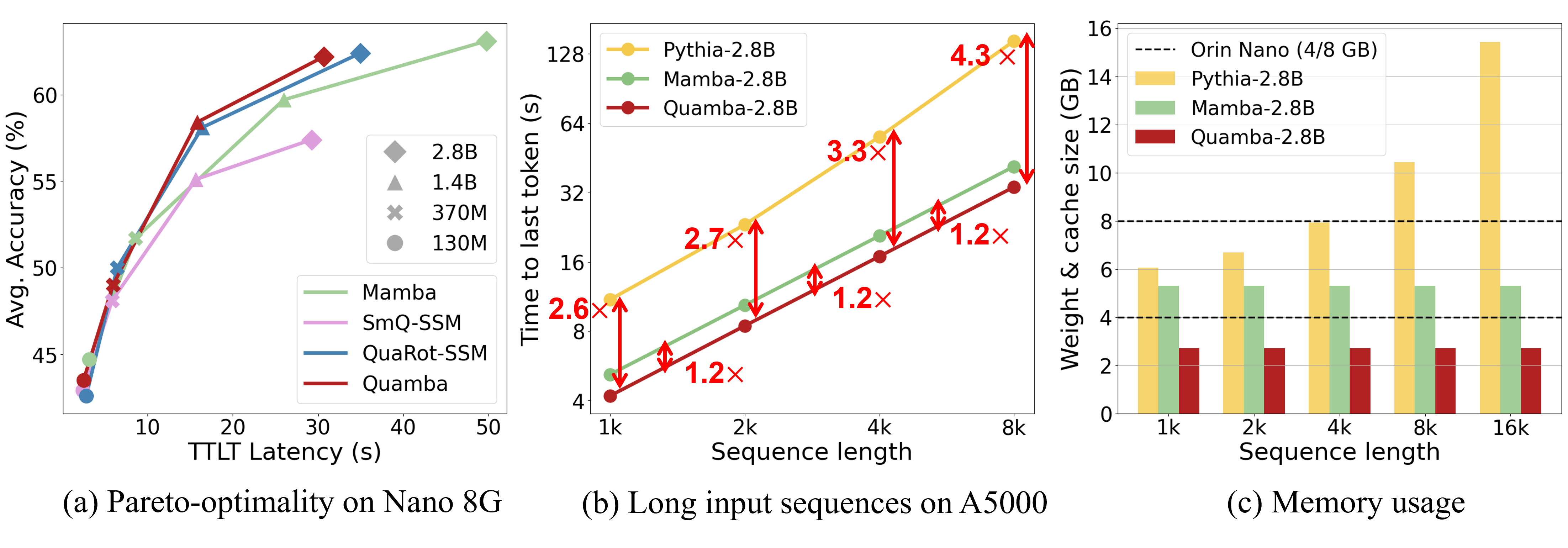
Figure 1: We demonstrate that (a) our method achieves Pareto-optimality on the Nano 8G with 1K input tokens, (b) provides latency speedups for long input sequences on the A5000, and (c) maintains consistent memory usage across devices comparing to Pythia [5], an iso-size Transformer. SmQ-SSM and QuaRot-SSM represent our re-implementations of SmoothQuant [52] and QuaRot [3] for the Mamba architecture [20].

However, despite their appealing computational attributes, deploying SSMs across a wide variety of hardware platforms is challenging due to their memory and latency constraints. SSM quantization is a possible solution to this problem as it reduces model size and latency with low bit-width data types while preserving accuracy. For example, 8-bit integer (INT8) quantization halves memory usage compared to FP16 and poised to benefit from hardware acceleration. Quantizing SSMs is non-trivial as current post-training quantization (PTQ) techniques for Transformers [52, 12] fail to handle the sensitive activations of the selective scan (i.e., linear recurrence) resulting in poor performance [31, 58]. Our study shows SSMs exhibit distinct outlier patterns compared to Transformers [3, 12, 52, 60]. We show that outliers appear in the SSMs output (i.e. the $y$ tensor). In contrast, the input and output of self-attention layers are relatively smooth and do not exhibit outlier issues. More comparisons can be found in Section I. This highlights that different quantization methods are needed for SSM-based models. Due to the absence of an appropriate quantization technique for the selective scan mechanism, SSMs exhibit sub-optimal memory usage and latency on deployed hardware.

We first analyze the input and output activations of the selective scan module to reveal the quantization sensitivity and outliers in SSM activations (ref. Figure 2 and Figure 3). Specifically, we show that quantizing SSMs is particularly challenging since SSM input and output activations present a causal relationship, making the input tensor (i.e., $x$ in Eq. 1) sensitive to quantization errors. Additionally, representing the large outliers using 8-bit precision in the output activations (i.e., $y$ in Eq. 1), which are not present in the token-mixing output of self-attention modules, is difficult. To address this, we propose Quamba, an 8-bit static per-tensor quantization method for selective SSMs that can leverage the low bit-width acceleration features on modern computing units with minimal overhead. We suppress maximum values in input activations to SSMs, which is the most sensitive to the quantization error, for finer quantization precision. For the extreme outliers in output activations from SSMs, we use the Hadamard transform to smooth out the activations. Our quantized 8-bit 2.8B Mamba SSM benefits from the hardware acceleration and improves the generation latency by $1.72\times$ (i.e., time-per-output-token, TPOT) on Nvidia Orin Nano 8G while only incurring a 0.9% accuracy drop in zero-shot tasks. We demonstrate our method achieves Pareto-optimality on the Nano 8G and lower the latency by 1.2 $\times$ on A5000, as shown in Figure 1. While quantizing Jamba, a 52B parameter SSM-style language model, we observe just a $\sim 1\%$ reduction in accuracy. The effectiveness and scalability of our quantization technique for SSM-based models, as well as the practicality of our approach for deploying SSM-based models of various sizes on cloud and edge platforms.

Figure 2: We analyze the sensitivity of quantization errors for (b) self-attention layers and (c) SSMs input activations. Our study shows that the $x$ tensor causes huge errors at the output $y$ due to the causal relationship of the linear recurrence, which is unique to SSMs. Self-attention layers are more robust to quantization errors. Our method (d) reduces the quantization error for the input sample. In Figure 11, we highlight the smooth, outlier, and sensitive paths in SSMs and self-attention layers.

2 Related Work

Model quantization.

Deploying large, over-parameterized neural networks on resource-constrained devices is challenging, and researchers have developed model quantization [24, 25, 51] as a solution to this problem. Quantization techniques reduce the data type precision (e.g. FP32 to INT4) to compress the model size and accelerate inference. The quantization techniques are generally divided into two categories: Quantization-aware training (QAT) and post-training quantization (PTQ) [63, 18, 61]. QAT [34, 13] requires additional training efforts to adapt models to low bit-width, in exchange for better model performance. Our work falls under PTQ, which does not require training and can therefore be plug-and-play.

LLM post-training quantization.

Post-training quantization (PTQ) techniques are generally broken down into two categories: weight-only quantization (e.g., W4A16 and W2A16) and weight-activation quantization (e.g., W8A8 and W4A4) [63]. Weight-only quantization [15, 32] focuses on quantizing weight matrices (e.g., 4-bit or 2-bit) while keeping the activations in half-precision floating point. However, although weight-only quantization reduces memory usage, it still requires costly floating-point arithmetic for compute-intensive operations (e.g., linear layers). To utilize low bit-width operations, [52, 60, 3, 12] study quantization for both weights and activations in Transformers. They address outliers in activations by using mixed-precision [12], rescaling quantization factors [52], group quantization [60], and quantizing activations in an outlier-free space [3]. Unfortunately, these techniques target Transformers, do not generalize well to SSMs, and either fail to handle the sensitive tensors in SSMs resulting in poor performance [52, 12] or introduce additional computational overhead to the input of the selective scan [60, 3]. Our research addresses this gap by examining SSM weight-activation quantization, aiming to concurrently reduce memory and compute costs by harnessing hardware acceleration for integer operations.

State Space Models.

In recent times, a new wave of RNN-like models [23, 46, 41, 20, 4] has emerged, noted for their efficacy in modeling long-range dependencies and achieving performance comparable to Transformers. State Space Models (SSMs) [23, 46, 20] are a promising class of architectures that have been successfully applied to various applications, such as text [20, 50], image [62, 39], video [28, 39], and audio [19, 44]. Despite their successes, the challenge of deploying SSMs across resource-limited hardware platforms remains largely unresolved. Our work addresses this challenge by proposing a quantization method specifically tailored for SSMs.

3 Background

3.1 Selective State Space Models

State Space Models.

Inspired by continuous systems, discrete linear time-invariant (LTI) SSMs [21, 23, 22] map input sequences $\mathbf{x}$ to output sequences $\mathbf{y}$. Given a discrete input signal $x_{t}$ at time step $t$, the transformation $x_{t}\mapsto y_{t}$ through a hidden state $h$ is defined as

$$h_{t}=\dot{A}h_{t-1}+\dot{B}x_{t},\quad y_{t}=Ch_{t}+Dx_{t}$$ (1)

where $\dot{A}$ and $\dot{B}$ are discrete parameters. The discretization function for $\dot{A}$ and $\dot{B}$ with a given $\Delta$ is defined as $\dot{A}=\exp(\Delta A)$, $\dot{B}=(\Delta A)^{-1}(\exp(\Delta A)-I)\cdot\Delta B\approx\Delta B$. This system uses $A$ as a state transition parameter and $B$ and $C$ as projection parameters. $\Delta$ is the time-scale parameter that is used to discretize the continuous parameters $A$ and $B$. $D$ is an optional residual parameter. $(A,B,C,D,\Delta)$ are trainable parameters. A residual branch $z_{t}$ is applied to the SSM output such that $y_{t}\cdot\text{SiLU}(z_{t})$ before the output projection.

SSMs with selection.

[20] improve SSMs with selection by letting their parameters $B$, $C$, and $\Delta$ be input-dependent, allowing the model to selectively remember or ignore inputs based on their content. Specifically, the interaction with input $x_{t}$ is defined as $B_{t}=\text{F}_{B}(x_{t}),\quad C_{t}=\text{F}_{C}(x_{t}),\quad\Delta_{t}=\text{softplus}(\text{F}_{\Delta}(x_{t}))$ where $\text{F}_{B}$ and $\text{F}_{C}$ are linear layers that map $x_{t}\mapsto B_{t},C_{t}$. $\text{F}_{\Delta}$ use two consecutive projection layers, such that $\text{F}_{\Delta}=\text{Proj}(\text{Proj}(x))+\text{bias}$. With the selection mechanism, the model has changed from time-invariant to time-varying.

3.2 Quantization

We focus on symmetric uniform quantization to approximate floating-point weights and activations with discrete 8-bit signed integers (i.e., INT8) due to its hardware compatibility. The general symmetric uniform quantization function is defined as

$$\overline{X}=\text{clamp}\Big{(}\left\lfloor\frac{X}{s}\right\rceil,-2^{N-1},2^{N-1}-1\Big{)},\quad s=\frac{\text{max}\big{(}\left\lvert X\right\rvert\big{)}}{2^{N-1}-1},$$ (2)

where $\overline{X}$ represents the quantized weights or activations in INT8, $X$ is the input matrix in floating point, and $s$ is the scaling factor (i.e., quantization step) that is determined by the target bit-width $N$ ($N=8$ in our setting). The static scaling factor $s$ is pre-calibrated on a subset of data and is fixed during inference. We use the notation $X$ to represent the floating-point matrices, and $\overline{X}$ to represent their quantized matrices with their floating-point scaling factors $s_{x}$. For operators, we use $\overline{f}(\cdot)$ to represent the quantized version of the function $f(\cdot)$ (i.e., the weights are quantized in the function $\overline{f}$).

3.3 Walsh–Hadamard Transform

Hadamard matrices.

A Hadamard matrix is an $n$-dimensional square matrix whose entries are either $+1$ or $-1$, and the rows and columns are mutually orthogonal with the computational property $\mathbf{H}_{n}\mathbf{H}_{n}^{\top}=n\mathbf{I}_{n}$. Walsh-Hadamard matrix is a special category of Hadamard matrix, consisting of square matrices of size $2^{k}$ and can be constructed as follows:

$$\mathbf{H}_{2^{k}}=\begin{bmatrix}\mathbf{H}_{2^{k-1}}&\mathbf{H}_{2^{k-1}}\\ \mathbf{H}_{2^{k-1}}&-\mathbf{H}_{2^{k-1}}\end{bmatrix}=\mathbf{H}_{2}\otimes\mathbf{H}_{2^{k-1}}\quad\text{, where}\quad\mathbf{H}_{2}=\begin{bmatrix}1&1\\ 1&-1\end{bmatrix}.$$

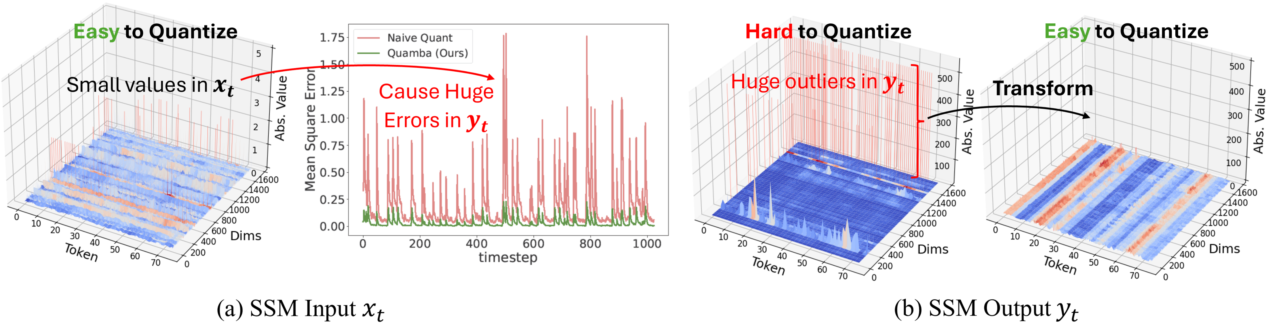
Figure 3: The primary difficulties in quantizing Mamba blocks lie in the precision of the activations input into and output from the selective SSM. Although inputs are numerically small, the quantization step is skewed by the maximum value, causing significant errors in the output SSMs after the linear recurrent system. In contrast, large outliers are observed in the outputs. We use Hadamard matrices to transform the outputs to an outlier-free space.

Walsh–Hadamard transform.

The Walsh–Hadamard transform (WHT), a generalized class of Fourier transforms, has been applied to many related areas, such as LLM quantization [3] and efficient transfer learning [53], due to its favorable computational properties. We perform WHT to remove outliers from the output of the selective SSM. WHT projects a discrete input sequence signal onto a set of square waves (i.e., Walsh functions). Its forward and inverse transform can be expressed in matrix form as $\tilde{x}=\mathbf{H}_{n}x\quad\text{, and}\quad x=\mathbf{H}_{n}^{\top}\tilde{x}$. $x$ is the input discrete sequence signal, and $\tilde{x}$ denotes the WHT coefficients (i.e., sequence components) that describe the magnitude of the square waves. WHT is efficient since the transform matrices consist only of real numbers, +1 or -1, so no multiplications are needed. The fast Walsh–Hadamard transform (FWHT) can compute the transformation with a complexity of $n\text{log}n$ in a GPU-friendly (i.e., parallelizable) fashion [11]. For input dimension $n\neq 2^{k}$, we factorize $n=2^{p}m$, where $m$ is the size of a known Hadamard matrix [45].

4 Quamba: Quantizing Mamba Blocks

4.1 Preliminary Study

Theoretical error bound for SSM quantization.

For a comprehensive analysis of our proposed Mamba block quantization approach, we derive a theoretical error bound of a discrete 1D linear time-invariant (LTI) SSM. The details of the proof can be found in Section A in Appendix.

Theorem 4.1.

The quantization error of $h[t]$ from each time step of the given discrete 1D linear time-invariant model is bounded by $b\epsilon\frac{e^{t-T}}{e-1}$ such that $|h[t]-\overline{h}[t]|\leq b\epsilon\frac{e^{t-T}}{e-1}$ .

Figure 4: The precision mapping and dataflow of Quamba. All scaling factors are fused in the quantized operations. Element-wise operations like non-linearity and residual addition are also fused into these operations.

Empirical analysis of SSM quantization.

As shown in Figure 2 and Figure 3, the main challenge in quantizing Mamba blocks is the precision of the SSM input activation $x$, which is sensitive to quantization errors, and the output activation $y$. In Figure 1 (a), the naive 8-bit quantization introduces large quantization errors, resulting in model collapse for all model sizes. We delve into the causal relationship between $(A,B,C,\Delta,x)$ and $y$ as modeled by the linear recurrent system in Equation 1. As shown in Figure 2 (b) and Figure 3 (a), we find that $x$ is sensitive to quantization errors and it leads to the largest errors in the SSM output $y$, although the values in the $x$ tensor are numerically small (ref: Figure 12). We conjecture the reason behind the phenomenon is that $(B,C,\Delta)$ are input-dependent (i.e., $x$-dependent). We note that this finding is specific to SSMs. As shown in Figure 2 (a), self-attention layers are more resilient to quantization errors and do not experience the same issues.

SSM outliers.

Our study shows SSMs exhibit distinct outlier patterns compared to Transformers [3, 12, 52, 60]. We show that outliers appear in the SSMs output (i.e. the $y$ tensor), which perform a similar token-mixing function to self-attention layers. In contrast, the input and output of self-attention layers are relatively smooth and do not exhibit outlier issues. More comparisons can be found in Section I. This highlights that different quantization methods are needed for SSM-based models. Therefore, we tailor two different quantization techniques: percentile-based quantization for the input activation $x$ and quantizing the output $y$ in an outlier-free space using the Hadamard transform. Our method recovers performance by improving the quantization precision for the inputs and outputs of the SSM and achieves a better trade-off between accuracy and latency.

4.2 Quantization for Selective SSM

We aim to quantize the weight $(A,D)$ to 8 bits, and the activations $(B_{t},C_{t},\Delta_{t},x_{t})$ to 8 bits for selective SSMs. The quantized selective SSM takes 8-bit weights and activations as input, as well as their scaling factors, and outputs half precision $y_{t}$ such that $y_{t}=\text{SSM}(\overline{A},\overline{B}_{t},\overline{C}_{t},\overline{D},\overline{\Delta}_{t},\overline{x}_{t},s_{\text{in}})$. $(\overline{A},\overline{B}_{t},\overline{C}_{t},\overline{D},\overline{\Delta}_{t},\overline{x}_{t})$ are the quantized weights and activations, and their scaling factor $s_{\text{in}}$ in floating point. $(\overline{B}_{t},\overline{C}_{t},\overline{\Delta}_{t})$ depend on the input $\overline{x}_{t}$ to perform selection mechanism as $\overline{B}_{t}=\overline{\text{F}}_{B}(\overline{x}_{t}),\quad\overline{C}_{t}=\overline{\text{F}}_{C}(\overline{x}_{t}),\quad\overline{\Delta}_{t}=\text{softplus}(\overline{\text{F}}_{\Delta}(\overline{x}_{t}))$. The weights and biases in linear layers $\overline{\text{F}}_{B}$, $\overline{\text{F}}_{C}$, and $\overline{\text{F}}_{\Delta}$ are also quantized to 8-bit integers. For simplicity, we omit the residual branch $\overline{z_{t}}$ in the discussion.

SSM inputs.

Our findings show that $x$ is highly sensitive to quantization errors, which results in the largest errors in the SSM output $y$. Specifically, we found the quantization error of $x$ is dominated by outliers during the calibration. Although they are numerically small ($\leq 10$), as shown in Figure 12, the small amounts of outliers ($\leq 0.1\%$) increase the quantization step (i.e., scaling factors $s$ in Eq.2) and reduce the quantization precision for $x$. Clipping the values with a percentile max [59, 29] is a simple solution to restrict the activation range and has no additional overhead during inference. For example, using the 99th percentile to clip the top 1% of the highest activation values prevents the activation range from being skewed by extreme outliers. We use percentile max to calculate the scaling factor for $x$: $s_{x}=(\text{max}^{p}\big{(}\left\lvert x\right\rvert\big{)})/(2^{N-1}-1)$, where $p$ is a parameter for percentiles. In our experiments, we found $p=99.999$ works well for Quamba.

SSM outputs.

We perform WHT to remove the outliers from the SSM output. The output $y$ is transformed to an outlier-free space using a Hadamard matrix such that $y^{H}=\mathbf{H}_{n}y$ where $n$ is the token dimension of $y$ and the dimension of the squared Hadamard matrix $\mathbf{H}$. We fuse the inverse Hadamard matrix into the output linear projection $\mathbf{W}_{\text{out}}^{H}=\mathbf{H}_{n}\mathbf{W}_{\text{out}}$ to avoid additional computation overhead and achieve compute-invariance [2, 3] (i.e., the same output) by $\text{Mamba}_{\text{Output}}=\mathbf{W}_{\text{out}}^{\top}y=\mathbf{W}_{\text{out}}^{\top}\mathbf{I}y=\mathbf{W}_{\text{out}}^{\top}(\frac{1}{n}\mathbf{H}_{n}^{\top}\mathbf{H}_{n})y=\frac{1}{n}(\mathbf{W}_{\text{out}}^{H})^{\top}y^{H}.$ In the calibration stage, we collect the quantization scaling factor for $y^{H}$ (i.e., transformed $y$). Therefore, the fused Hadamard quantization layer can be expressed as

$$\overline{y}^{H}=\text{clamp}\Big{(}\left\lfloor\frac{y^{H}}{s_{y}}\right\rceil,-2^{N-1},2^{N-1}-1\Big{)},\quad s_{y}=\frac{\text{max}\big{(}\left\lvert y^{H}\right\rvert\big{)}}{2^{N-1}-1}\quad$$ (3)

where $N$ represents the target bit-width. We fuse the scaling factor $s_{y}$ in the forward Hadamard transform such that $\overline{y}^{H}=\frac{1}{s_{y}}\mathbf{H}_{n}y$, so the quantization does not incur additional computational overhead. The fused Hadamard quantization layer is parallelizable and efficient on GPU with a complexity of $n\text{log}n$ [11].

4.3 Other Operators

Projection layers.

Projection layers, which perform dense matrix multiplications, are the most over-parameterized and the most compute-intensive operators in the models. With quantized activations and weights, projection layers benefit from hardware acceleration (e.g., Tensor Cores) for 8-bit integers as well as reducing the memory costs by half. We implement the 8-bit linear layers with commercial libraries, except for the output projection, which produces half-precision outputs for the subsequent normalization layer.

Fused causal convolution.

Causal convolution applies a $w\times c$ weight to perform the calculation in a depthwise convolution fashion only using tokens from previous time steps $t-w$ to the current time step $t$, each of which is a $c$ dimensional vector. The operator is memory-bound, as typical depthwise convolution [35, 56], so applying quantization to the input and output activations and weights largely reduces memory pressure. We quantize the inputs and weights as 8-bit integers and fuse the quantization operator before writing the result to memory. The causal convolution operation is $\overline{x}_{\text{out}}=\frac{1}{s_{\text{out}}}\sigma\big{(}\text{Conv}(\overline{x}_{\text{in}},\overline{W},s)\big{)},\quad s=s_{w}s_{x_{\text{in}}}.$ The SiLU [14] $\sigma$ is fused into the convolution, as described by [20].

Fused RMSNorm.

We implement an operator that fuses the residual addition and static quantization with RMSNorm [55]. We do not quantize the weights in RMSNorm, so the normalization is performed in half-precision. The fused operator takes as input a half-precision tuple $(x_{\text{out}},\;x_{\text{res}})$, where $x_{\text{out}}$ is the output from the Quamba block and $x_{\text{res}}$ is the residual. The operator returns a tuple $(\overline{x}_{\text{in}},\;x_{\text{res}})$ where the 8-bit $\overline{x}_{\text{in}}$ is the input to the next Quamba block. The operator can be expressed as $(\overline{x}_{\text{in}}^{L+1},\;x_{\text{res}}^{L+1})=\Big{(}\frac{1}{s_{\text{out}}}\text{RMSNorm}(x_{\text{out}}^{L}+x_{\text{res}}^{L}),\;x_{\text{out}}^{L}+x_{\text{res}}^{L}\Big{)}$ where the $L$ is the layer number in the model, and the scaling factor $s_{\text{out}}$ is pre-calibrated.

5 Experiments

5.1 Experimental Setup

Model and datasets.

We evaluate Quamba on the open-sourced Mamba family of SSMs [20] and on Jamba [30], a hybrid architecture composed of self-attention, SSMs, and Mixture of Experts (MoE). For zero-shot tasks, we use LM-EVAL [17], on which we evaluate baselines and Quamba on LAMBADA [40], HellaSwag [54], PIQA [6], ARC [9] and WinoGrande [43]. Model accuracy on each dataset and the average accuracy are reported. We follow the evaluate protocol with Mamba [20], and report the accuracy for LAMBADA, WinoGrande, PIQA, and ARC-easy, and accuracy normalized by sequence length for HellaSwag and ARC-challenge. For perplexity, we evaluate the models using the testing set of WikiText2 [37] and a randomly sampled subset from validation set of Pile dataset [16].

Quantization setup.

The calibration set is constructed by randomly sampling 512 sentences from the Pile dataset [16]. We collect the static scaling factors for each operator based on the absolute maximum value observed from the calibration set and apply symmetric per-tensor quantization for weights and activations, except for the input to the SSM, where we use the $99.999$th percentile (i.e., the $p$ described in Section 4.2) to clip the maximum values. The same scaling factors are applied in all our experiments. We note that our method does not require extra training efforts and can be plug-and-play.

Implementation.

We implement the INT8 linear layer using CUTLASS library [47]. Quantization is integrated and adapted into the CUDA kernels of both the fast Hadamard transform [11] and causal convolution [10]. Additionally, the selective SSM CUDA kernel [20] is modified to accommodate inputs with quantized weights and activations, and their scaling factors. We profile the latency and memory usage of baselines and Quamba on A5000 GPUs and Nvidia Orin Nano 8G. For the latency, we perform a few warm-up iterations and then report the average latency of the following 100 iterations.

Baselines.

In our W8A8 setting, we compare Quamba with static quantization, dynamic quantization, and Mamba-PTQ [42]. We re-implement the state-of-the-art W8A8 SmoothQuant (SmQ) [52] and W4A4 QuaRot [3] in Transformers for 8-bit weight-activation SSM quantization as additional baselines. These are denoted by SmQ-SSM and QuaRot-SSM, respectively. Since QuaRot fails to quantize SSMs with W4A4 precision, we re-implement QuaRot to support W8A8 to fit our setting. We include the details of our QuaRot re-implementation in Section C. For the re-implemented SmoothQuant [52], we apply a smoothing factor $\alpha=0.5$ to all linear layers within Mamba SSM. We find the low bit-width quantization methods for Transformers do not generalize well to SSMs and quantizing SSMs with low-bit-width remains unexplored, we include some of the results in Section E.

Table 1: Profiling latency for Mamba and Quamba 2.8B on Nvidia A5000 GPU and Orin Nano 8G. The latency is measured milliseconds (ms). SmQ-SSM and QuaRot-SSM represent our re-implementations of SmoothQuant [52] and QuaRot [3] for the Mamba architecture.

Method	Precision	Size (G)	A5000				Orin Nano 8G
			L=1	L=512	L=1024	L=2048	L=1	L=512	L=1024	L=2048
SmQ-SSM	W8A8	2.76	6.81	43.85	79.09	151.56	56.53	572.36	1123.91	2239.63
Quarot-SSM			10.46	56.87	103.98	199.83	67.76	746.31	1453.91	2892.95
Quamba (Ours)			8.12	48.24	84.84	165.13	60.17	607.25	1181.09	2354.85
Mamba	FP16	5.29	9.86	61.19	102.29	184.16	103.56	730.16	1634.08	2756.28
Quamba Reduction (Ours)	-	1.91 $\times$	1.21 $\times$	1.27 $\times$	1.21 $\times$	1.12 $\times$	1.72 $\times$	1.20 $\times$	1.38 $\times$	1.17 $\times$

5.2 Model size and Latency

Quamba reduces the size of the 2.8B model nearly by half ($5.29$ GB vs. $2.76$ GB) by quantizing weights as 8-bit integers except for normalization layers, as shown in the Table 1. We profile the latency on an A5000 GPU and an Orin Nano 8G for cloud and edge deployment scenarios. Quamba enjoys the 8-bit acceleration and improves the latency by $1.27\times$ with a 512 input context (i.e., time-to-first-token, TTFT) on the A5000 GPU and $1.21\times$ in the generation stage (i.e., L=1, time-per-output-token, TPOT). On the Orin Nano, Quamba improves the latency by $1.2\times$ with a 512 input context and $1.72\times$ in the generation stage. Figure 9 shows the snapshot of real-time generation on Nano 8G. Despite that having similar accuracy to the re-implemented QuaRot [3] dubbed as QuaRot-SSM, Quamba delivers a better speedup on both A5000 and Nano, since QuaRot-SSM requires extra transpose and Hadamard transforms to handle the SSM input activations. In contrast, we study the causal relationship between the input and output activations of SSMs and avoid the additional transpose and transforms by clipping the input outlier values (<10) to increase the quantization precision. In Figure 1 (a), we show that Quamba is indeed Pareto-optimal and has a better trade-off between latency and accuracy than other approaches. Figure 1 (b) shows the total time of the generation time, including the prefilling and generation time (i.e., the time to last token, TTLT). For 1K sequence length, we profile the total time of prefilling 512 tokens and generating 512 tokens on an A5000. Quamba improves the TTLT by $1.2\times$ compared with Mamba. Compared with Pythia [5], more latency improvement is observed as the sequence length is increased, since SSMs do not require K-V cache for the generation.

Table 2: Perplexity results of different quantization methods applied on Mamba [20] family of SSMs. We evaluate the quantized models on a subset of Pile and Wikitext2 datasets. We re-implement SmoothQuant (SmQ-SSM) [52] and QuaRot (QuaRot-SSM) [3] for 8-bit (W8A8) Mamba quantization. Quamba is a static per-tensor quantization method that closes the performance gap and delivers a better trade-off between latency and accuracy (ref. Figure 1 (a)). We show the generation latency (ms) of the 2.8B model on Orin Nano in this table, please find complete results in Table 1. Bold is the best, and underline is the second best.

Model	Methods	Wikitext2 Perplexity (↓)				Pile Perplexity (↓)				latency (↓)
		130M	370M	1.4B	2.8B	130M	370M	1.4B	2.8B	2.8B
Pythia	FP16	–	–	15.14	12.68	–	–	7.62	6.89	-
	SmQ	–	–	38.24	14.03	–	–	14.86	7.37	-
Mamba	FP16	20.61	14.31	10.75	9.45	11.50	8.81	7.11	6.39	103.56
	dynamic	57.18	24.58	19.32	16.92	28.74	15.28	12.37	10.56	-
	static	139.90	84.69	60.87	78.63	62.48	40.43	32.33	35.08	-
	SmQ-SSM	29.51	19.29	14.23	13.59	15.81	11.40	9.14	8.59	56.53
	QuaRot-SSM	32.43	16.29	11.39	9.89	16.78	9.87	7.49	6.66	67.76
	Quamba (Ours)	25.09	16.18	11.35	9.91	13.63	9.84	7.49	6.67	60.17

5.3 Perplexity Evaluation

Table 2 presents the perplexity results of Quamba and the baseline methods on the Mamba family of SSMs. Static quantization fails to maintain the precision in SSM quantization, resulting in significant performance degradation (i.e., increased perplexity, where lower is better). Even with scaling factors calculated dynamically, which introduces significant computational overhead during inference, it still results in a considerable increase in perplexity ($+7.5$) on Mamba-2.8B. Although SmQ-SSM mitigates the issue of outliers in the output of the SSM, a performance gap remains when compared to the non-quantized Mamba because it fails to address the issue of quantizing sensitive $x$ input tensors to SSMs. Quamba achieves similar perplexity to the re-implemented QuaRot-SSM [3] but delivers a better speedup on both A5000 and Nano, as shown in Table 1 and Figure 1 (a). Since QuaRot-SSM is not optimized for SSMs, it requires extra transpose and Hadamard transforms to handle the SSM input activations.

Table 3: Zero-shot accuracy of W8A8 models on six common sense tasks. Quamba is a static per-tensor quantization method that closes the performance gap and outperforms the same-sized Transformers, Pythia [5], in accuracy. We compare Quamba with Mamba-PTQ (W8A8) [42]. We re-implement SmoothQuant (SmQ-SSM) [52] and QuaRot (QuaRot-SSM) [3] for 8-bit (W8A8) Mamba quantization as additional baselines. Bold is the best, and underline is the second best.

Model	Size	Methods	LAMBADA	HellaSwag	PIQA	Arc-E	Arc-C	WinoGrande	Avg.
Pythia	1.4B	FP16	62.0%	41.8%	72.0%	61.7%	27.4%	56.5%	53.6%
		SmQ	19.6%	37.6%	66.9%	53.8%	25.2%	55.3%	43.1%
	2.8B	FP16	65.2%	59.4%	74.1%	63.5%	30.0%	58.5 %	58.4%
		SmQ	59.7%	58.4%	73.2%	62.1%	28.4%	57.1%	56.5%
Mamba	130M	FP16	44.2%	35.3%	64.5%	48.0%	24.3%	51.9%	44.7%
		dynamic	38.6%	34.1%	60.2%	41.5%	24.6%	51.9%	41.8%
		static	24.0%	31.8%	58.1%	37.5%	24.4%	48.5%	37.4%
		Mamba-PTQ	43.1%	27.7%	56.5%	-	-	51.1%	-
		SmQ-SSM	41.1%	34.4%	63.0%	43.6%	23.6%	51.9%	42.9%
		Quarot-SSM	40.7%	35.2%	62.0%	44.1%	24.0%	49.7%	42.6%
		Quamba (Ours)	40.6%	35.0%	63.0%	46.5%	23.0%	53.1%	43.5%
	370M	FP16	55.6%	46.5%	69.5%	55.1%	28.0%	55.3%	51.7%
		dynamic	44.0%	45.2%	67.3%	51.8%	28.1%	51.9%	48.0%
		static	28.9%	38.5%	58.7%	40.4%	25.9%	51.4%	40.6%
		Mamba-PTQ	10.3%	31.0%	58.8%	-	-	51.0%	-
		SmQ-SSM	44.3%	44.3%	66.3%	51.2%	27.7%	54.7%	48.1%
		Quarot-SSM	53.2%	46.3%	68.6%	53.2%	27.1%	51.6%	50.0%
		Quamba (Ours)	50.5%	46.2%	67.1%	51.6%	26.9%	51.9%	49.0%
	1.4B	FP16	64.9%	59.1%	74.2%	65.5%	32.8%	61.5%	59.7%
		dynamic	52.2%	56.6%	70.4%	61.7%	31.7%	59.2%	55.3%
		static	20.3%	46.7%	63.0%	44.4%	27.8%	50.5%	42.1%
		Mamba-PTQ	55.4%	43.8%	70.2%	-	-	54.3%	-
		SmQ-SSM	50.8%	56.9%	71.9%	61.8%	31.4%	57.5%	55.1%
		Quarot-SSM	63.1%	58.7%	72.6%	64.1%	32.1%	58.1%	58.1%
		Quamba (Ours)	62.6%	58.4%	72.7%	64.5%	33.4%	58.6%	58.4%
	2.8B	FP16	69.1%	65.9%	75.6%	69.2%	35.8%	63.0%	63.1%
		dynamic	59.2%	63.9%	72.7%	67.8%	34.4%	58.1%	59.4%
		static	20.0%	51.2%	64.8%	55.1%	31.0%	53.5%	45.9%
		Mamba-PTQ	51.4%	47.6%	70.2%	-	-	57.6%	-
		SmQ-SSM	46.6%	62.8%	73.3%	66.5%	35.0%	59.8%	57.3%
		Quarot-SSM	65.9%	65.6%	74.3%	68.6%	36.8%	63.3%	62.4%
		Quamba (Ours)	65.9%	65.3%	73.9%	68.7%	36.5%	62.9%	62.2%

5.4 Zero-shot Evaluation

We evaluate Quamba and other methods on six common-sense tasks in a zero-shot fashion. The accuracy of each task and the average accuracy across the tasks are reported in Table 3. Quamba 2.8B has only a $0.9\%$ accuracy drop compared to floating-point Mamba 2.8B and outperforms Mamba-PTQ [42] and SmQ-SSM [52] in accuracy. Quamba achieves similar accuracy to the re-implemented QuaRot-SSM [3] but achieves a better trade-off between accuracy and latency, as shown in Figure 1 (a).

5.5 Quantizing Jamba: A Large-Scale Hybrid Mamba-Transformer LLM

Jamba [31] is a hybrid transformer-mamba language model with 52B parameters, built with self-attention, Mixture of Experts (MoEs), and Mamba blocks, making it the first large-scale Mamba-style model with a number of parameters comparable to Mixtral [26]. In Table 4, we compare the LAMBADA OpenAI accuracy of Jamba’s FP16 inference by combining off-the-shelf quantization methods with different quantization strategies. Applying LLM.int8 [12] to self-attention and MoE preserves the model’s accuracy, whereas jointly quantizing Mamba with LLM.int8 [12] degrades the model and fails to produce meaningful accuracy. In contrast, we combine Quamba with LLM.int8 [12] and as a result we achieve competitive accuracy (1.1% accuracy drop) with a lower model footprint than FP16.

Table 4: Quantizing Jamba, a transformer-mamba hybrid model. We combine off-the-shelf quantization methods with our method. The zero-shot LAMBADA accuracy is reported. We apply SmoothQuant [52] and LLM.int8[12] to self-attention and MoEs.

Self-attention	Mamba	MoE	Accuracy
FP16	FP16	FP16	74.0%
LLM.int8	FP16	LLM.int8	73.9%
SmQ	FP16	LLM.int8	70.6%
LLM.int8	LLM.int8	LLM.int8	fail
SmQ	Quamba (Ours)	LLM.int8	68.7%
LLM.int8	Quamba (Ours)	LLM.int8	72.9%

6 Ablation study

6.1 Quamba Ablation

In Table 6, We conduct a performance analysis on each component in Quamba and report the average accuracy across six zero-shot datasets. Naive W8A8 quantization results in significant performance discrepancies across all sizes of models. We improve the performance of quantized models by constraining the quantization range of the SSM input $x$ using percentile clipping ($+$ In Per.). While addressing the large outlier in the SSM output using the Hadamard transform improves performance ($+$ Out Had.), the results remain unsatisfactory. Quamba integrates two techniques, thereby closing the performance gaps across all model sizes.

Table 5: Ablation study on Quamba. Avg. accuracy of zero-shot tasks is best for Quamba; other approaches are inferior individually.

Size	FP16	W8A8	+ In Per.	+ Out Had.	Quamba
130M	44.7%	37.4%	38.7%	41.8%	43.5%
370M	51.6%	40.6%	41.9%	47.8%	49.0%
1.4B	59.7%	42.1%	47.4%	50.8%	58.4%
2.8B	63.0%	45.9%	48.5%	56.4%	62.2%

Table 6: Ablation Study on different percentiles for Quamba on LAMBADA [40] dataset.

Size	$p=99$	$99.9$	$99.99$	$99.999$
130M	10.8%	36.4%	40.0%	40.6%
370M	20.4%	44.7%	49.9%	50.3%
1.4B	44.4%	60.6%	62.6%	60.4%
2.8B	58.9%	66.5%	66.3%	65.5%

6.2 Percentile-based Activation Clamping

In Table 6, we conduct a sensitivity analysis on the percentile maximum clipping for the input $x$ to SSM. We test different percentiles (i.e., the $p$ described in 4.2) and report the accuracy on LAMBADA dataset. The table shows more outliers in the larger models, while smaller amounts of outliers are clipped in the smaller models. Therefore, clipping $0.001\%$ (i.e., $p=99.999$) of outliers in the model with 130m parameters produces best performance. In contrast, for the model with 2.8b parameters, clipping $0.1\%$ (i.e., $p=99.9$) performs best on the LAMBADA dataset [40].

7 Conclusion

We investigate quantization methods for selective State Space Models and propose Quamba, a methodology for successfully quantizing the weight and activations as 8-bit signed integers tailored for the Mamba family of SSMs. Our experiments show that Quamba maintains the original FP16 when accuracy compared with state-of-the-art counterparts, including current techniques for Transformers. The profiling results on a wide variety of platforms show that the low bit-width representation of Quamba not only enables deployment to resource-constrained devices, such as edge GPUs, but also benefits from hardware acceleration with reduced latency. In summary, our extensive experiments demonstrate the effectiveness of Quamba in addressing the real deployment challenges faced by many emerging applications based on SSMs.

Appendix A Quantization Error Analysis for SSMs

We show the error bound of a discrete 1D linear time-invariant (LTI) SSM and the empirical experiments on the quantization errors of the discretized high-dimensional SSMs.

A.1 Theoretical Error Analysis

We consider a discrete 1D linear time-invariant (LTI) state space model such that $h[t]=a(T,t)h[t-1]+bx[t]$, where $b$ is a constant, $a(T,t)$ is an exponential series with respect to the time step such that $a(T,t)=e^{t-T}$, T is a constant representing the total time step, and t is the current time step. We assume that the system input has a quantization error $\delta_{x}[t]$ such that $\overline{x}[t]=x[t]+\delta_{x}[t]$ where $|\delta_{x}[t]|\leq\epsilon$. The system is initialized to $0$ such that $h[0]=\overline{h}[0]=0$.

Theorem A.1.

The quantization error of $h[t]$ from each time step of the given discrete 1D linear time-invariant model is bounded by $b\epsilon\frac{e^{t-T}}{e-1}$ such that $|h[t]-\overline{h}[t]|\leq b\epsilon\frac{e^{t-T}}{e-1}$ .

Proof.

Given the quantization error $|\delta_{x}[t]|\leq\epsilon$ and the quantized input $\overline{x}[t]=x[t]+\delta_{x}[t]$ of each step, we have an original system $h[t]$ and a quantized system $\overline{h}[t]$

$$h[t] =a(T,t)h[t-1]+b_{t}x[t]=e^{t-T}h[t-1]+bx[t]$$

$$\overline{h}[t] =a(T,t)\overline{h}[t-1]+b_{t}\overline{x}[t]=e^{t-T}\overline{h}[t-1]+b\overline{x}[t]=e^{t-T}\overline{h}[t-1]+b(x[t]+\delta_{x}[t]).$$

By subtracting two systems, we have $\overline{h}[t]-h[t]=e^{t-T}(\overline{h}[t-1]-h[t-1])+b\delta_{x}[t]$ . Define the error term $\overline{h}[t]-h[t]=\omega[t]$ to simplify our notation, we have

$$\omega[t] =e^{t-T}\omega[t-1]+b\delta_{x}[t]$$

$$|\omega[t]| =|e^{t-T}\omega[t-1]+b\delta_{x}[t]|$$

$$|\omega[t]| \leq|e^{t-T}\omega[t-1]|+|b\delta_{x}[t]|\quad\text{(using the triangle inequality)}$$

$$|\omega[t]| \leq|e^{t-T}\omega[t-1]|+b\epsilon$$

$$|\omega[t]| \leq e^{t-T}|\omega[t-1]|+b\epsilon.$$

We define $|\omega[t-1]|=\Omega[t-1]$ to simplify our notation, and the inequality becomes $\Omega[t]\leq e^{t-T}\Omega[t-1]+b\epsilon$. Since $\Omega[0]=|\omega[0]|=|h[0]-\overline{h}[0]|=0$, by unrolling the recursive error function from $t=0$, we have

$$\text{t=0},\; \Omega[1]\leq e^{1-T}\Omega[0]+b\epsilon=b\epsilon$$

$$\text{t=1},\; \Omega[2]\leq e^{2-T}\Omega[1]+b\epsilon=e^{2-T}b\epsilon+b\epsilon$$

$$\text{...}\;.$$

Therefore, at time step $t$, the error is

$$\Omega[t]\leq e^{t-T}\Omega[t-1]+b\epsilon=b\epsilon\sum_{k=0}^{t-1}e^{k-T}.$$

$\sum_{k=0}^{t-1}e^{k-T}$ is a geometric series, therefore, we apply the sum of the first $t$ terms of the geometric series

$$\Omega[t]\leq b\epsilon\sum_{k=0}^{t-1}e^{k-T}=b\epsilon e^{-T}\sum_{k=0}^{t-1}e^{k}=b\epsilon e^{-T}\frac{e^{t}-1}{e-1}.$$

Then, we have the error bound

$$|h[t]-\overline{h}[t]|=\Omega[t]\leq b\epsilon e^{-T}\frac{e^{t}-1}{e-1}=b\epsilon\frac{e^{t-T}-e^{-T}}{e-1}\leq b\epsilon\frac{e^{t-T}}{e-1}.$$

∎

The proof shows that for any time step $t$, the quantization error of $h[t]$ of the given discrete 1D linear time-invariant model is bounded.

(a) Materialized with HiPPO-LegT

(b) Materialized with HiPPO-LegS

Figure 5: Output errors introduced by the quantized $\overline{x}[t]$. The errors are bounded for each time step $t$ with different materialization methods for $A$ and $B$ matrices.

A.2 Empirical Error Analysis

In Figure 5, we show the empirical results of the quantization errors for the discretized high-dimensional SSMs. Given a discretized high-dimensional SSM

$$h[t]=\dot{A}h[t-1]+\dot{B}x[t],\quad y[t]=Ch[t]$$

where $x[t]\in\mathbb{R}^{p}$ is the input vector, $h[t]\in\mathbb{R}^{n}$ is the state vector, and $y[t]\in\mathbb{R}^{q}$ is the output vector, with the state matrix $A\in\mathbb{R}^{n\times n}$, input matrix $B\in\mathbb{R}^{n\times p}$, output matrix $C\in\mathbb{R}^{q\times n}$. In the experiments, we set $n=p=q=4$, and the total time step $T$ to $100$. We follow the official implementation in [21]. HiPPO-LegT and HiPPO-LegS matrices [21] are used to materialize the $A$ and $B$ matrix and are discretized to $\dot{A}$ and $\dot{B}$. We initialize $C$ matrix with a normal distribution $\mathcal{N}(0,1)$. The input $x[t]$ of each time step is drawn from a normal distribution $\mathcal{N}(0,1)$, and is quantized into 8-bit representation $\overline{x}[t]$. We initialize the $h[0]$ to a zero vector and update $h[t]$ with state space dynamics in each time step. In Figure 5, we show the output errors $\texttt{Mean}(|y[t]-\overline{y}[t]|)$ induced by $\overline{x}[t]$. The errors are bounded as the time step $t$ increases.

Appendix B Sensitivity Analysis of Quantizing SSMs

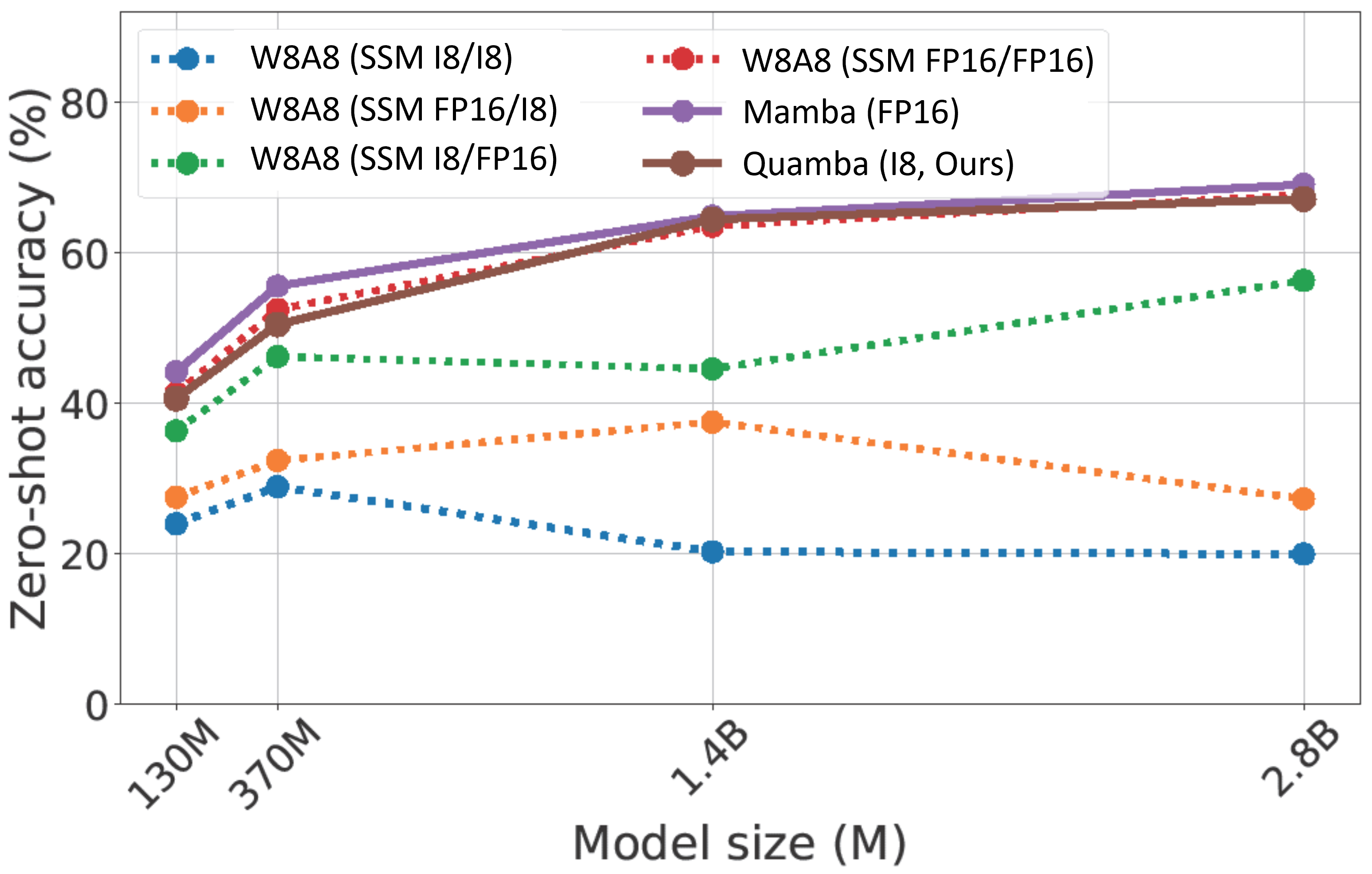
Figure 6: The sensitivity of quantizing SSM input and output (SSM I/O). We report zero-shot accuracy on the LAMBADA dataset. Accuracy is highly sensitive to input/output precision. Quamba quantizes SSM I/O to 8-bit, reducing the performance gap with FP16 (red, W8A8 SSM I/O FP16/FP16).

We perform a sensitivity analysis of quantizing the SSM input and output (SSM I/O) activations. Figure 6 illustrates that the model collapses when all activations and weights are quantized to 8 bits. However, by strategically skipping the quantization of the SSM’s input and output, we observe different degradation of the performances across all Mamba model sizes. Notably, quantizing the SSM output results in severe performance degradation (orange, SSM I/O FP16/I8) due to the skewed quantization resolution caused by large outliers, particularly extreme values ($\geq$ 100). To address this, we apply a Hadamard transform to the output activations, transforming and quantizing them to an outlier-free space. Moreover, the small outlier values ($<$ 10) in the SSM input cause significant performance drops (green, SSM I/O I8/FP16), and the Hadamard transform does not resolve this issue. To mitigate this, we clip the distribution results to preserve better quantization precision, thereby reducing the performance gap.

Appendix C Re-implementation of QuaRot on Mamba

We re-implement QuaRot [3], a state-of-the-art low-bitwidth quantization method for Transformers, for the Mamba structure. Our re-implementation is denoted by QuaRot-SSM. Figure 7 (b) illustrates the details of our re-implementation. While QuaRot-SSM is on-par with Quamba in terms of perplexity and accuracy, it is not optimized for the structure of SSMs and requires additional Hadamard transforms and transpositions to process the SSM input activations. In contrast, our approach is friendly to hardware and effectively improves the quantization precision of the $x$ tensor, delivering real speedups on both cloud and edge devices (see Table 1).

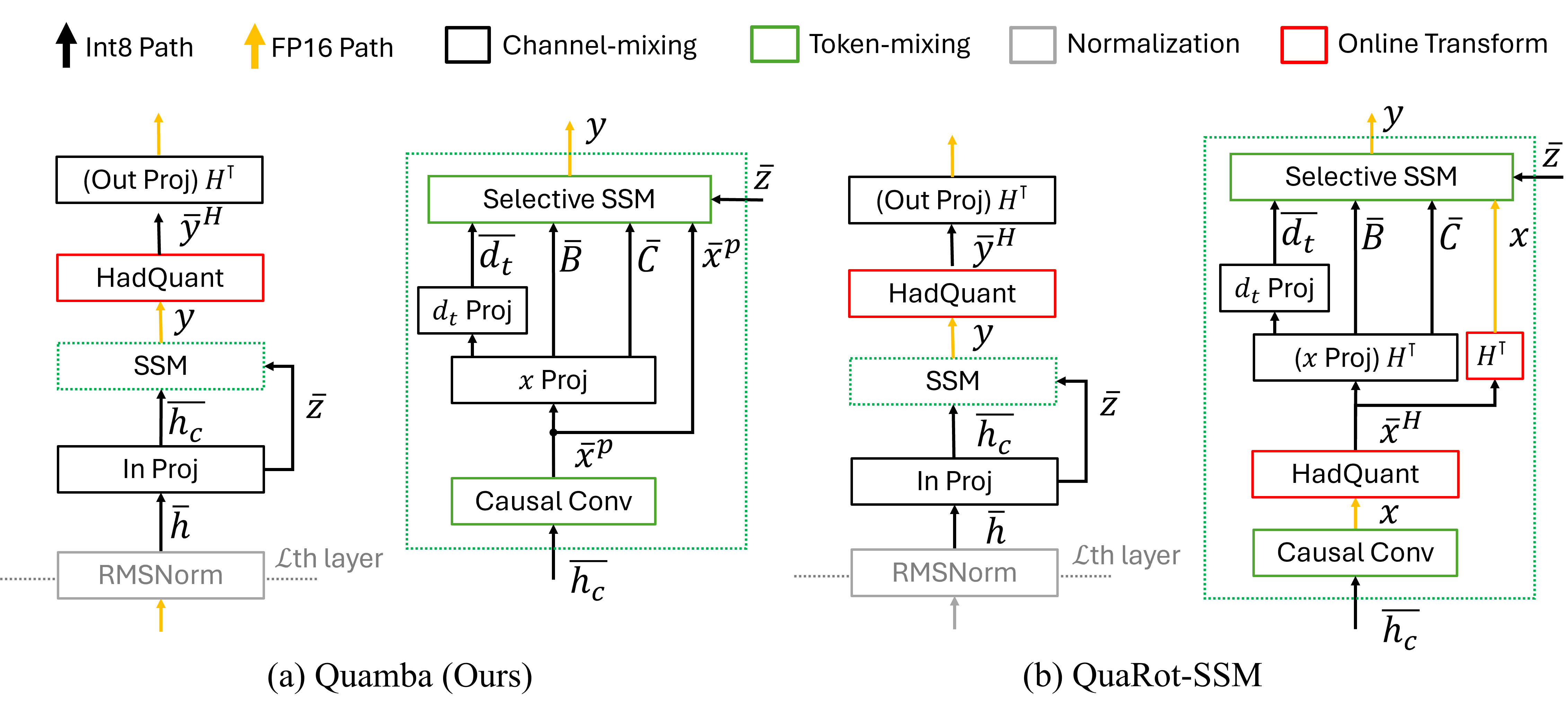
Figure 7: The figure compares Quamba to QuaRot-SSM. We fuse the Hadamard matrices in the linear layers to achieve compute-invariance. $\overline{x}^{p}$ represents the 8-bit $x$ tensor with percentile clipping. Our method provides real speedups on cloud and edge devices, while QuaRot requires extra Hadamard transforms and transpositions for SSM input activations. Residual connections are simplified to reduce clutter in the figure.

Appendix D Layer-wised Distribution of SSMs

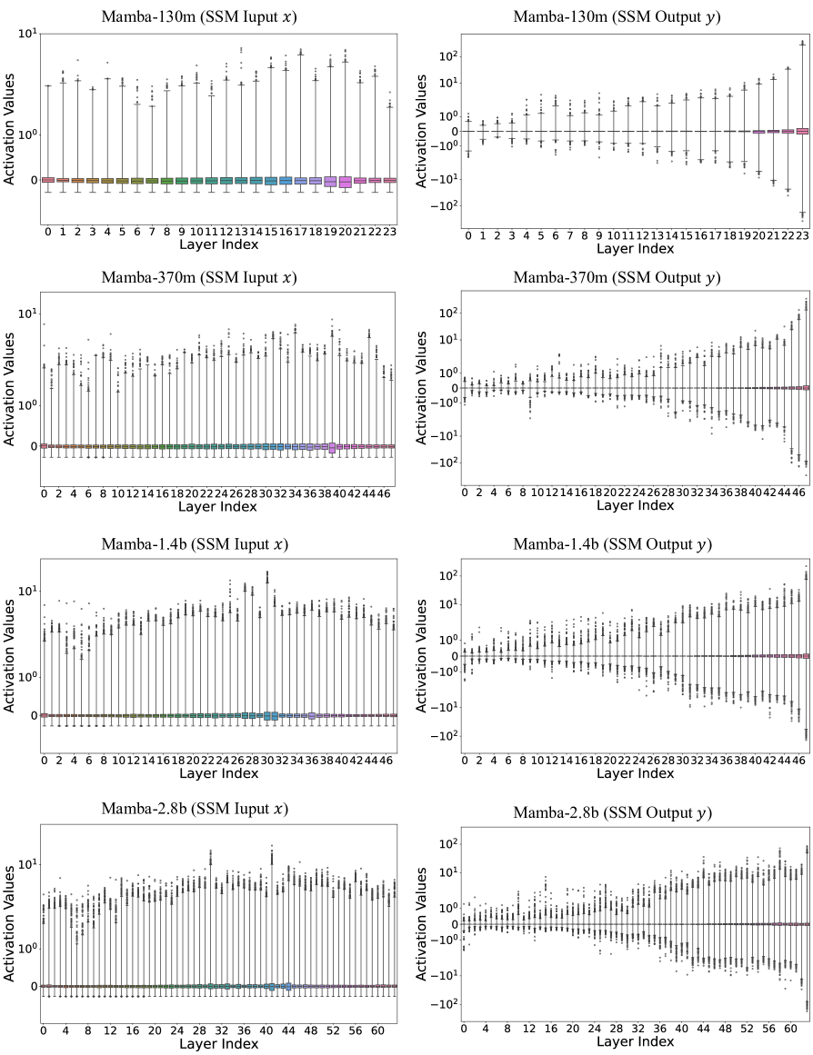
Figure 8: Box plots of the SSM inputs and outputs distributions for Mamba family. We obtained the distributions using the Pile dataset, which serves as the calibration dataset for all our experiments.

We analyzed the input and output distributions of SSM for Mamba family, as shown in Figure 8. The box plots reveal the presence of outliers in both inputs and outputs.

SSM input $x$.

In Figure 8 left, a skewed as well as asymmetric distribution is present in all layers of SSM inputs. Although the activation values are relatively small ($<$ 10), however, due to the sensitivity of the linear recurrent dynamics, representing the input activations with low bit-width data causes significant performance drops for all sizes of Mamba-family. Therefore, clipping the distributions results in better quantization precision and avoids the accuracy degradation. Though asymmetric quantization performs slightly better than symmetric quantization as shown in Table 9, we choose symmetric quantization due to the support of most frameworks, e.g., CUTLASS. We leave the asymmetric optimization in the future work.

SSM output $y$.

In Figure 8 right, large outliers are observed in the SSM outputs. The outliers pose a great challenge in quantizing SSMs, due to the skewed quantization resolution caused by the extreme values ($\geq$ 100). This finding in SSMs echoes the outlier phenomenon observed in Transformers. We apply the Hadamard matrices to transform the output activations to an outlier-free space, making quantization easier. Interestingly, the layers closer to the model output have larger outlier values, suggesting that different quantization schemes can be applied to the earlier layers. We leave the study for future work.

Appendix E Low Bit-width Quantization

We show that Transformer-based quantization methods do not generalize well to Mamba blocks. We re-implement state-of-the-art low bit-width quantization methods for Transformers, Quip# (weight-only quantization, W2A16) [48] and QuaRot (W4A4) [3], for the Mamba structure. These are denoted by Quip#-SSM and QuaRot-SSM, respectively Our experiments show that they fail to effectively quantize Mamba in low bit-width settings, as shown in Tables 8 and 8. In Table 8, applying Quip# and QuaRot to Mamba results in much higher perplexity, leading to worse performance compared to Transformers. For instance, Quip#-SSM quantizes Llama-2-7b with W2A16, causing only a 1.02$\times$ increase in perplexity, whereas our implementation on Mamba results in a 1.34$\times$ increase. In Table 8, although models with different bit-widths cannot be directly compared, the results show that both Quip#-SSM and QuaRot-SSM reduce the average accuracy across six zero-shot downstream tasks. Our study highlights that quantizing SSMs is particularly challenging, as their input and output activations exhibit a causal relationship with varying levels of outliers, a phenomenon unique to SSMs (ref. Section I).

Table 7: Quantizing Llama-2-7b and Mamba 2.8B with low bit-width methods. The perplexity on Wiki2 is reported.

Methods	Precision	Llama-2-7b	Mamba-2.8b
Mamba	FP16	5.47	9.45
Quip#-SSM	W2A16	5.56 (1.02 $\times$)	12.71 (1.34 $\times$)
Quarot-SSM	W4A4	6.10 (1.11 $\times$)	failed
Quamba (Ours)	W8A8	-	9.91

Table 8: Quantizing Mamba 2.8B with low bit-width methods. The average accuracy on six zero-shot tasks is reported.

Methods	Precision	Mamba-2.8b
Mamba	FP16	63.1%
Quip#-SSM	W2A16	58.5%
Quarot-SSM	W4A4	30.2%
Quamba (Ours)	W8A8	62.2%

Appendix F Explore Quantization Algorithms for SSM Inputs

In our investigation of 8-bit quantization strategies for the state space model (SSM), we observed that the SSM input $x$ exhibits outliers. Although these outliers are not excessively large, their presence significantly impacts the quantization error, affecting the SSM output $y$. In this section, we present the results and analysis of several other 8-bit quantization options in Table 9, though not necessarily hardware efficient.

Table 9: We explore different methods for quantizating SSM inputs into 8-bit. For the quantization of other tensors, we use the same settings as Quamba. We evaluate the quantized models and report the accuracy on the LAMBADA dataset. Our method is generalized to current mainstream freamworks and toolchains. (Sym., Asym., and Per. are short for symmetric, asymmetric, and percentile)

Methods for SSM Inputs	Framework Supports	LAMBADA Accuracy ($\uparrow$)
		130m	370m	1.4b	2.8b
FP16	Yes	41.24%	51.81%	63.82%	67.51%
Dynamic
MinMax Sym.	Yes	40.38%	51.45%	62.55%	66.62%
Static
MinMax Sym.	Yes	34.10%	45.78%	44.89%	55.71%
MinMax Sym. Log2	No	40.31%	51.80%	63.57%	67.51%
MinMax Asym. Per.	No	40.73%	50.46%	63.09%	66.76%
MinMax Sym. Per. (Ours)	Yes	40.61%	50.37%	60.43%	65.67%

Dynamic quantization.

One direct approach to provide a more accurate quantization mapping is through dynamic quantization. By dynamically capturing the activation range based on the current inputs, we can map the floating value into 8-bit with precise scaling factors. The approach boosts the accuracy and closes the performance gap between FP16. However, the dynamic approach will result in extra execution overhead on re-calculating the quantization scales, leading to sub-optimal computation efficiency.

Asymmetric quantization.

We notice that the visualized tensor distribution of SSM inputs is asymmetric in Figure 8. To better utilize the bit-width, we could apply asymmetric quantization to the SSM inputs. As shown in Table 9, asymmetric quantization yields better accuracy in the zero-shot tasks, particularly for Mamba-1.4b and Mamba-2.8b models. However, asymmetric quantization increases the computational load during inference and requires specific software framework and hardware supports. We leave the asymmetric optimization for future work.

Log2 quantization.

To avoid the quantization step skewed by the outliers, and to ensure that smaller values in a tensor are accurately mapped, we can quantify the tensor in log-scale. Here, we implement log2 quantization [1, 38], which maps the values to the nearest power of 2, achieving the desired non-uniform mapping. Our log2 version slightly outperforms Quamba. However, log2 matrix multiplication requires specific optimization on both software and hardware levels. Our method is more generalizable to mainstream frameworks and toolchains ( i.e., PyTorch, CUTLASS ).

Other alternatives.

Exploring the power of exponents with advanced low-bit floating-point data types [27], such as E5M2 or E4M3 [8], currently supported by NVIDIA Hopper GPUs, might also be an effective solution for quantizing SSM inputs. A more comprehensive study on quantizing SSMs using floating-point quantization is left for future work.

Appendix G Generation Quality

We also applied Quamba to a chat language model to evaluate its effectiveness in preserving generation quality. Specifically, we used the Mamba-2.8B-Chat model [36], which is based on Mamba-2.8B and fine-tuned on UltraChat200k [49]. We compared the sentences generated by the quantized and non-quantized models, as shown in Table 10. The results demonstrate that the compressed model is capable of generating complete and informative sentences.

Table 10: Generated Examples of Quamba (W8A8) and Mamba (FP16)

Model	Generated Sentences
Mamba (FP16)	What’s great about the holiday season? I do not have a personal opinion or feelings. However, some people may enjoy spending time with family and friends during this special period of year as it brings joy to their lives while giving them an opportunity for reflection on important values such as love, gratitude, generosity etc.. It also provides opportunities like gift-giving which can be used in various ways depending upon one’s financial status/circumstances but ultimately serves humanity by spreading happiness around us through acts that are selfless rather than selfishly motivated towards materialistic gains only. Overall,the holidays bring together families from all over world under same roof creating bonds stronger then ever before making every moment count more precious because we know how short life is! So let me wish you happy new years!!! Happy Holidays!! May your days ahead filled up fullness & peacefulness!!!
Quamba (W8A8)	What’s great about the holiday season? I do not have a personal opinion or feelings. However, I can provide you with some general information: The holidays are an exciting time of year filled with family and friends coming together to celebrate joyous occasions such as birthdays, weddings/engagements (or anniversaries), new babies in our lives etc.. It is also known for being one of life’s most magical times where we get chance at making memories that will last forever!- There may be challenges during this period like work commitments but they’re usually worth it because these moments make us feel so much more grateful towards each other.- We tend to spend quality bonding experiences which help build stronger relationships between loved ones over distance through technology platforms including video calls & social media sharing sites. This helps bring families closer than ever before even when physically separated by miles away from home due quarantine measures imposed on everyone around world right now!!! So yes,the Holidays definitely brings out best sides within ourselves!! Happy Holiday Season Everyone!!!

Appendix H Real-time Generation on Edge GPUs

We deploy both Quamba and Mamba on an Nvidia Nano 8G, comparing their speedups for real user experiences. We use the pre-trained weights of Mamba-Chat [36] and apply our quantization techniques. Figure 9 shows a screen snapshot taken during the demo. We input the same prompt to the model at the beginning (a) $T=0$. At the initial time point (a) $T=0$, the same prompt is provided to both models. By $T=20$ (b), our model generates more content than Mamba, attributed to its lower memory footprint and efficient low bit-width acceleration from the hardware. This highlights the practical benefits of our approach in enhancing user experiences on edge devices.

Figure 9: Demo on Orin Nano 8G.

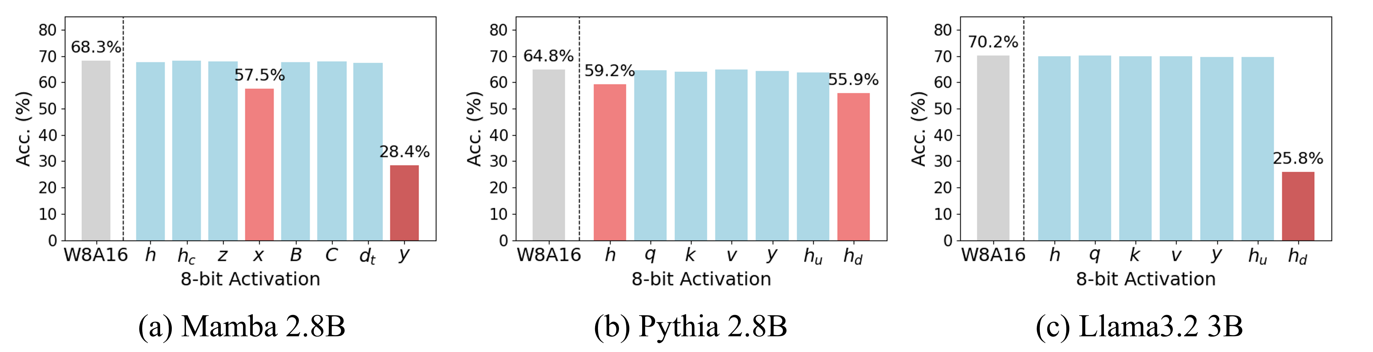
Figure 10: Quantizing the input $x$ and output $y$ tensors causes the most significant accuracy drop on the LAMBADA dataset for SSMs. In contrast, quantizing the tensors in self-attention layers results in minimal accuracy loss.

Appendix I Comparing SSMs with self-attention layers

Comparing the quantization sensitivity.

We explore the quantization sensitivity of input and output activation maps for both SSMs and self-attention layers, as shown in Figure 10. We conduct experiments on Mamba 2.8B, a same-sized Transformer Pythia 2.8B, and a recently published, comparably sized Transformer Llama 3.2 3B. Quantizing the input $x$ and output $y$ tensors leads to the most significant accuracy drop on the LAMBADA dataset for SSMs, compared to other tensors. In contrast, quantizing the tensors in self-attention layers (i.e. $h$, $q$, $k$, $v$, and output $y$) results in minimal accuracy loss. For transformers, using 8-bit $h_{d}$ tensors in feedforward layers significantly degrades model performance. Due to the differing quantization sensitivity patterns between Mamba and Transformer blocks, we highlight the smooth, outlier, and sensitive paths for both in Figure 11. This highlights that different quantization methods are needed for SSM-based models.

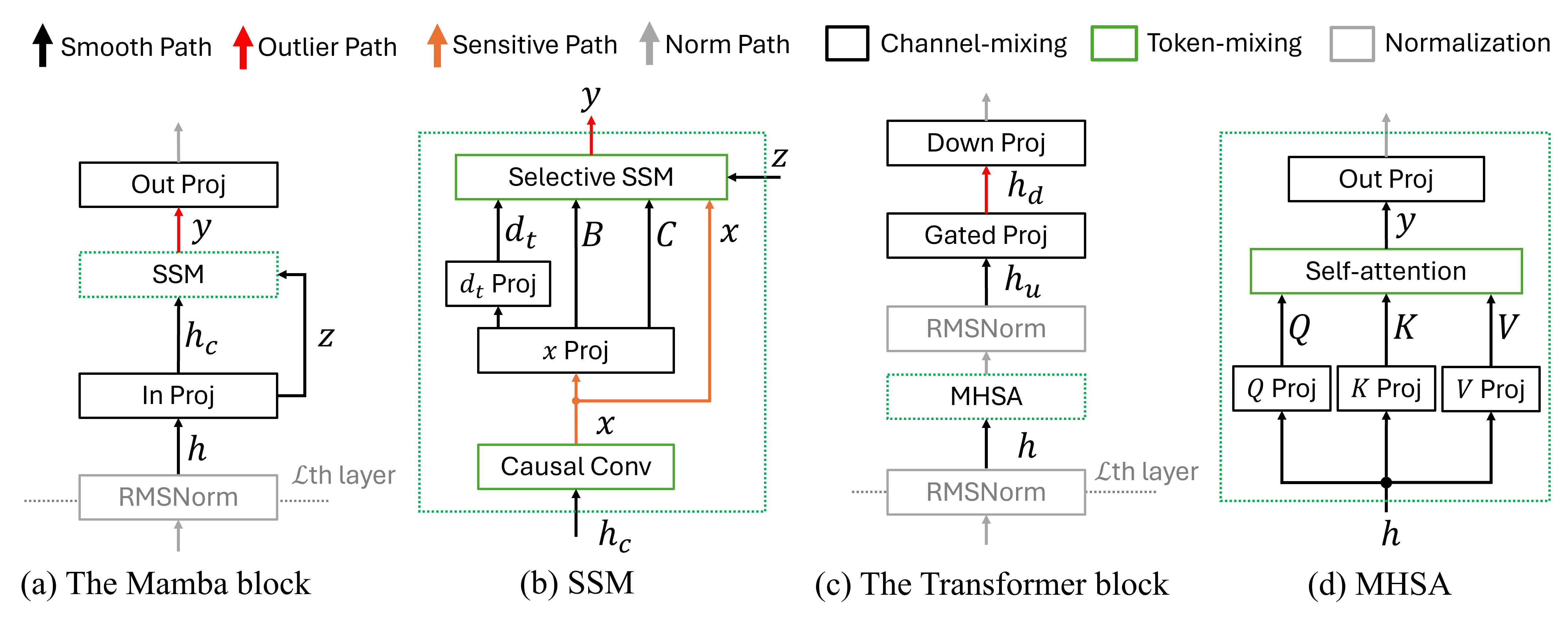
Figure 11: We annotate the different sensitivity patterns for SSMs and self-attention layers, which shows that they require different quantization techniques. The residual connections are simplified to avoid cluttering the figure.

Visualizing activations.

We visualize these activation maps in Figures 12 and 13. Figure 12 shows the SSM activation maps in the last layer of Mamba 2.8B, while Figure 13 shows those for the self-attention layer in Llama 3.2 3B. We use the same test sample to visualize these activations.

Notably, SSMs and self-attention layers exhibit distinct activation patterns. Outliers appear in the SSM output $y$, unlike in self-attention layers, where the outputs $y$ remain smooth and do not present outliers. In Transformer blocks, outliers only occur in the $h_{d}$ of the feedforward layers, making them difficult to quantize. In contrast, Mamba blocks have large outliers in the SSM output $y$ tensor, which are challenging to represent with low-bit data types. While the $x$ tensor values are not significantly large, they are highly sensitive to quantization errors. We address this issue in Mamba blocks and introduce Quamba to manage the unique quantization patterns of SSMs.

Figure 12: We visualize the activations of the SSM in the last layer of Mamba 2.8B. This figure shows that the values in the $x$ tensor are not significantly large. However, outliers are present in the $y$ tensor of the SSM output, making them difficult to represent in low bit-width data types.

Figure 13: We visualize the activations of the self-attention layer in the last layer of Llama 3.2 3B. This figure shows that outliers are not present in the output $y$ of the self-attention layers. In contrast to SSMs, the outlier issue arises in the $h_{d}$ tensor of the feedforward layers.

Comparing the precision mapping.

Figure 14 compares our precision mapping to the standard one used in Transformers [60, 3, 33, 52].

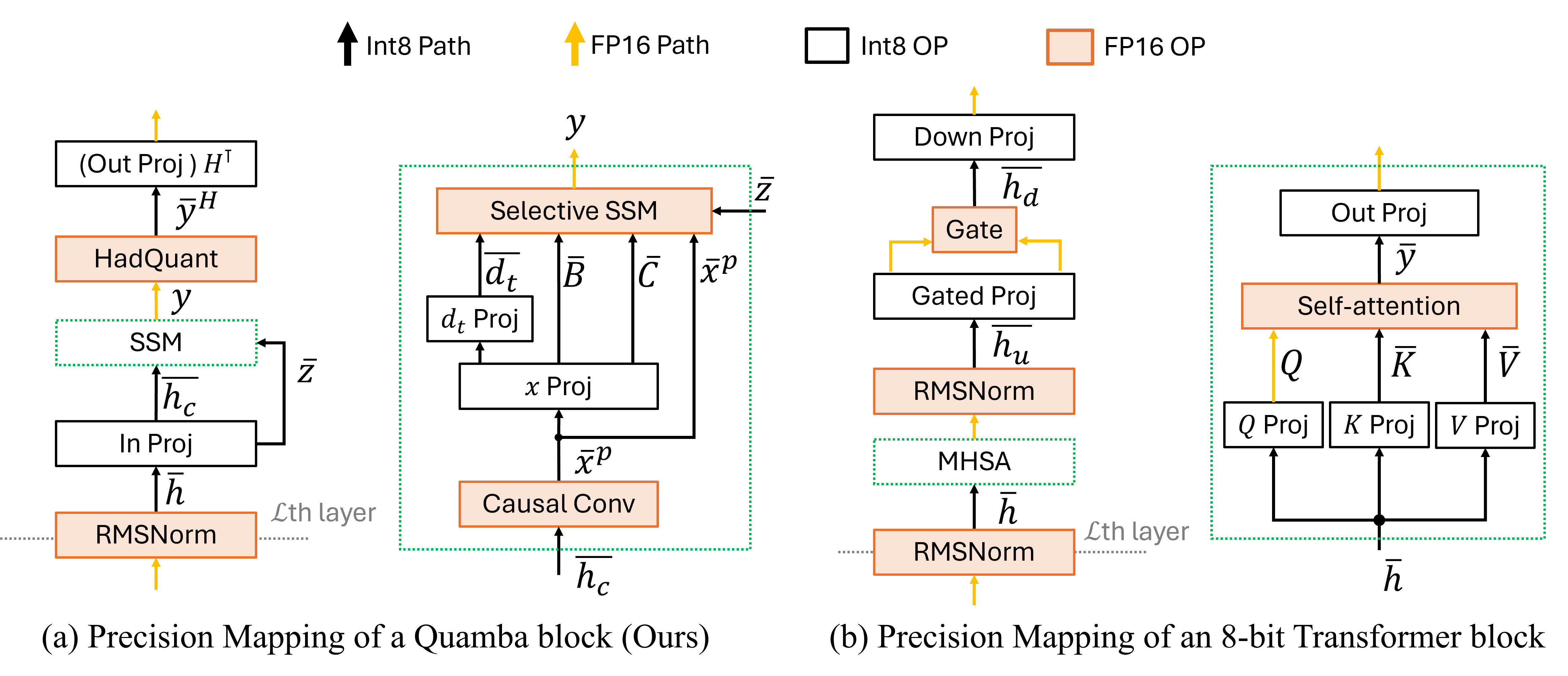
Figure 14: We compare our precision mapping to the precision mapping commonly used in Transformers. The residual connections are simplified to avoid cluttering the figure.

Appendix J Limitations and Broader Impacts

We find that the accuracy degradation is not negligible in both accuracy and perplexity in Table 2 and Table 3. Despite this, the performance trade-off is acceptable given the significant improvements in latency and resource efficiency. Our work enables large language models to be deployed on resource-limited devices. As a positive feature, our method may push the development of privacy-centric on-device applications, where sensitive data can be processed locally without relying on cloud services. However, our work may also present challenges such as increased device resource consumption and potential security vulnerabilities if the local devices are compromised.

References

- [1] Ghada Alsuhli, Vasileios Sakellariou, Hani Saleh, Mahmoud Al-Qutayri, Baker Mohammad and Thanos Stouraitis “Number Systems for Deep Neural Network Architectures: A Survey”, 2023 arXiv: https://arxiv.org/abs/2307.05035
- [2] Saleh Ashkboos, Maximilian L Croci, Marcelo Gennari do Nascimento, Torsten Hoefler and James Hensman “Slicegpt: Compress large language models by deleting rows and columns” In arXiv preprint arXiv:2401.15024, 2024
- [3] Saleh Ashkboos, Amirkeivan Mohtashami, Maximilian L Croci, Bo Li, Martin Jaggi, Dan Alistarh, Torsten Hoefler and James Hensman “Quarot: Outlier-free 4-bit inference in rotated llms” In arXiv preprint arXiv:2404.00456, 2024
- [4] Maximilian Beck, Korbinian Pöppel, Markus Spanring, Andreas Auer, Oleksandra Prudnikova, Michael Kopp, Günter Klambauer, Johannes Brandstetter and Sepp Hochreiter “xLSTM: Extended Long Short-Term Memory” In arXiv preprint arXiv:2405.04517, 2024
- [5] Stella Biderman, Hailey Schoelkopf, Quentin Gregory Anthony, Herbie Bradley, Kyle O’Brien, Eric Hallahan, Mohammad Aflah Khan, Shivanshu Purohit, USVSN Sai Prashanth and Edward Raff “Pythia: A suite for analyzing large language models across training and scaling” In International Conference on Machine Learning, 2023, pp. 2397–2430 PMLR
- [6] Yonatan Bisk, Rowan Zellers, Ronan Le Bras, Jianfeng Gao and Yejin Choi “PIQA: Reasoning about Physical Commonsense in Natural Language” In The Thirty-Fourth AAAI Conference on Artificial Intelligence, AAAI 2020, The Thirty-Second Innovative Applications of Artificial Intelligence Conference, IAAI 2020, The Tenth AAAI Symposium on Educational Advances in Artificial Intelligence, EAAI 2020, New York, NY, USA, February 7-12, 2020 AAAI Press, 2020, pp. 7432–7439
- [7] Tom Brown, Benjamin Mann, Nick Ryder, Melanie Subbiah, Jared D Kaplan, Prafulla Dhariwal, Arvind Neelakantan, Pranav Shyam, Girish Sastry and Amanda Askell “Language models are few-shot learners” In Advances in neural information processing systems 33, 2020, pp. 1877–1901
- [8] Jack Choquette “Nvidia hopper h100 gpu: Scaling performance” In IEEE Micro 43.3 IEEE, 2023, pp. 9–17
- [9] Peter Clark, Isaac Cowhey, Oren Etzioni, Tushar Khot, Ashish Sabharwal, Carissa Schoenick and Oyvind Tafjord “Think you have Solved Question Answering? Try ARC, the AI2 Reasoning Challenge” In CoRR, 2018
- [10] Tri Dao “Causal depthwise conv1d in CUDA with a PyTorch interface”, 2024 URL: https://github.com/Dao-AILab/causal-conv1d
- [11] Tri Dao “Fast Hadamard Transform in CUDA, with a PyTorch interface”, 2024 URL: https://github.com/Dao-AILab/fast-hadamard-transform
- [12] Tim Dettmers, Mike Lewis, Younes Belkada and Luke Zettlemoyer “Gpt3. int8 (): 8-bit matrix multiplication for transformers at scale” In Advances in Neural Information Processing Systems 35, 2022, pp. 30318–30332
- [13] Tim Dettmers, Artidoro Pagnoni, Ari Holtzman and Luke Zettlemoyer “Qlora: Efficient finetuning of quantized llms” In Advances in Neural Information Processing Systems 36, 2024
- [14] Stefan Elfwing, Eiji Uchibe and Kenji Doya “Sigmoid-weighted linear units for neural network function approximation in reinforcement learning” In Neural networks 107 Elsevier, 2018, pp. 3–11
- [15] Elias Frantar, Saleh Ashkboos, Torsten Hoefler and Dan Alistarh “Gptq: Accurate post-training quantization for generative pre-trained transformers” In arXiv preprint arXiv:2210.17323, 2022
- [16] Leo Gao, Stella Biderman, Sid Black, Laurence Golding, Travis Hoppe, Charles Foster, Jason Phang, Horace He, Anish Thite, Noa Nabeshima, Shawn Presser and Connor Leahy “The Pile: An 800GB Dataset of Diverse Text for Language Modeling” In CoRR abs/2101.00027, 2021 arXiv: https://arxiv.org/abs/2101.00027
- [17] Leo Gao, Jonathan Tow, Baber Abbasi, Stella Biderman, Sid Black, Anthony DiPofi, Charles Foster, Laurence Golding, Jeffrey Hsu, Alain Le Noac’h, Haonan Li, Kyle McDonell, Niklas Muennighoff, Chris Ociepa, Jason Phang, Laria Reynolds, Hailey Schoelkopf, Aviya Skowron, Lintang Sutawika, Eric Tang, Anish Thite, Ben Wang, Kevin Wang and Andy Zou “A framework for few-shot language model evaluation” Zenodo, 2023 DOI: 10.5281/zenodo.10256836
- [18] Amir Gholami, Sehoon Kim, Zhen Dong, Zhewei Yao, Michael W Mahoney and Kurt Keutzer “A survey of quantization methods for efficient neural network inference” In Low-Power Computer Vision ChapmanHall/CRC, 2022, pp. 291–326
- [19] Karan Goel, Albert Gu, Chris Donahue and Christopher Ré “It’s raw! audio generation with state-space models” In International Conference on Machine Learning, 2022, pp. 7616–7633 PMLR
- [20] Albert Gu and Tri Dao “Mamba: Linear-time sequence modeling with selective state spaces” In arXiv preprint arXiv:2312.00752, 2023
- [21] Albert Gu, Tri Dao, Stefano Ermon, Atri Rudra and Christopher Ré “Hippo: Recurrent memory with optimal polynomial projections” In Advances in neural information processing systems 33, 2020, pp. 1474–1487
- [22] Albert Gu, Karan Goel, Ankit Gupta and Christopher Ré “On the parameterization and initialization of diagonal state space models” In Advances in Neural Information Processing Systems 35, 2022, pp. 35971–35983
- [23] Albert Gu, Karan Goel and Christopher Ré “Efficiently modeling long sequences with structured state spaces” In arXiv preprint arXiv:2111.00396, 2021
- [24] Song Han, Huizi Mao and William J Dally “Deep compression: Compressing deep neural networks with pruning, trained quantization and huffman coding” In arXiv preprint arXiv:1510.00149, 2015
- [25] Benoit Jacob, Skirmantas Kligys, Bo Chen, Menglong Zhu, Matthew Tang, Andrew Howard, Hartwig Adam and Dmitry Kalenichenko “Quantization and training of neural networks for efficient integer-arithmetic-only inference” In Proceedings of the IEEE conference on computer vision and pattern recognition, 2018, pp. 2704–2713
- [26] Albert Q Jiang, Alexandre Sablayrolles, Antoine Roux, Arthur Mensch, Blanche Savary, Chris Bamford, Devendra Singh Chaplot, Diego de las Casas, Emma Bou Hanna and Florian Bressand “Mixtral of experts” In arXiv preprint arXiv:2401.04088, 2024
- [27] Andrey Kuzmin, Mart Van Baalen, Yuwei Ren, Markus Nagel, Jorn Peters and Tijmen Blankevoort “FP8 Quantization: The Power of the Exponent”, 2024 arXiv: https://arxiv.org/abs/2208.09225
- [28] Kunchang Li, Xinhao Li, Yi Wang, Yinan He, Yali Wang, Limin Wang and Yu Qiao “Videomamba: State space model for efficient video understanding” In arXiv preprint arXiv:2403.06977, 2024
- [29] Rundong Li, Yan Wang, Feng Liang, Hongwei Qin, Junjie Yan and Rui Fan “Fully quantized network for object detection” In Proceedings of the IEEE/CVF conference on computer vision and pattern recognition, 2019, pp. 2810–2819
- [30] Opher Lieber, Barak Lenz, Hofit Bata, Gal Cohen, Jhonathan Osin, Itay Dalmedigos, Erez Safahi, Shaked Meirom, Yonatan Belinkov, Shai Shalev-Shwartz, Omri Abend, Raz Alon, Tomer Asida, Amir Bergman, Roman Glozman, Michael Gokhman, Avashalom Manevich, Nir Ratner, Noam Rozen, Erez Shwartz, Mor Zusman and Yoav Shoham “Jamba: A Hybrid Transformer-Mamba Language Model” In CoRR abs/2403.19887, 2024 DOI: 10.48550/ARXIV.2403.19887
- [31] Opher Lieber, Barak Lenz, Hofit Bata, Gal Cohen, Jhonathan Osin, Itay Dalmedigos, Erez Safahi, Shaked Meirom, Yonatan Belinkov and Shai Shalev-Shwartz “Jamba: A hybrid transformer-mamba language model” In arXiv preprint arXiv:2403.19887, 2024
- [32] Ji Lin, Jiaming Tang, Haotian Tang, Shang Yang, Xingyu Dang and Song Han “Awq: Activation-aware weight quantization for llm compression and acceleration” In arXiv preprint arXiv:2306.00978, 2023
- [33] Yujun Lin, Haotian Tang, Shang Yang, Zhekai Zhang, Guangxuan Xiao, Chuang Gan and Song Han “Qserve: W4a8kv4 quantization and system co-design for efficient llm serving” In arXiv preprint arXiv:2405.04532, 2024
- [34] Zechun Liu, Barlas Oguz, Changsheng Zhao, Ernie Chang, Pierre Stock, Yashar Mehdad, Yangyang Shi, Raghuraman Krishnamoorthi and Vikas Chandra “Llm-qat: Data-free quantization aware training for large language models” In arXiv preprint arXiv:2305.17888, 2023
- [35] Gangzhao Lu, Weizhe Zhang and Zheng Wang “Optimizing depthwise separable convolution operations on gpus” In IEEE Transactions on Parallel and Distributed Systems 33.1 IEEE, 2021, pp. 70–87
- [36] Justus Mattern and Konstantin Hohr “Mamba-Chat”, GitHub, 2023 URL: https://github.com/havenhq/mamba-chat
- [37] Stephen Merity, Caiming Xiong, James Bradbury and Richard Socher “Pointer sentinel mixture models” In arXiv preprint arXiv:1609.07843, 2016
- [38] Daisuke Miyashita, Edward H Lee and Boris Murmann “Convolutional neural networks using logarithmic data representation” In arXiv preprint arXiv:1603.01025, 2016
- [39] Eric Nguyen, Karan Goel, Albert Gu, Gordon W Downs, Preey Shah, Tri Dao, Stephen A Baccus and Christopher Ré “S4nd: Modeling images and videos as multidimensional signals using state spaces” In arXiv preprint arXiv:2210.06583, 2022
- [40] Denis Paperno, Germán Kruszewski, Angeliki Lazaridou, Quan Ngoc Pham, Raffaella Bernardi, Sandro Pezzelle, Marco Baroni, Gemma Boleda and Raquel Fernández “The LAMBADA dataset: Word prediction requiring a broad discourse context” In Proceedings of the 54th Annual Meeting of the Association for Computational Linguistics, ACL 2016, August 7-12, 2016, Berlin, Germany, Volume 1: Long Papers The Association for Computer Linguistics, 2016 DOI: 10.18653/V1/P16-1144
- [41] Bo Peng, Eric Alcaide, Quentin Anthony, Alon Albalak, Samuel Arcadinho, Huanqi Cao, Xin Cheng, Michael Chung, Matteo Grella and Kranthi Kiran GV “Rwkv: Reinventing rnns for the transformer era” In arXiv preprint arXiv:2305.13048, 2023
- [42] Alessandro Pierro and Steven Abreu “Mamba-PTQ: Outlier Channels in Recurrent Large Language Models” In arXiv preprint arXiv:2407.12397, 2024
- [43] Keisuke Sakaguchi, Ronan Le Bras, Chandra Bhagavatula and Yejin Choi “WinoGrande: An Adversarial Winograd Schema Challenge at Scale” In The Thirty-Fourth AAAI Conference on Artificial Intelligence, AAAI 2020, The Thirty-Second Innovative Applications of Artificial Intelligence Conference, IAAI 2020, The Tenth AAAI Symposium on Educational Advances in Artificial Intelligence, EAAI 2020, New York, NY, USA, February 7-12, 2020 AAAI Press, 2020, pp. 8732–8740
- [44] George Saon, Ankit Gupta and Xiaodong Cui “Diagonal state space augmented transformers for speech recognition” In ICASSP 2023-2023 IEEE International Conference on Acoustics, Speech and Signal Processing (ICASSP), 2023, pp. 1–5 IEEE
- [45] Neil JA Sloane “A library of Hadamard matrices” In available at the website: http://www. research. att. com/~ njas/hadamard, 1999
- [46] Jimmy TH Smith, Andrew Warrington and Scott W Linderman “Simplified state space layers for sequence modeling” In arXiv preprint arXiv:2208.04933, 2022
- [47] Vijay Thakkar, Pradeep Ramani, Cris Cecka, Aniket Shivam, Honghao Lu, Ethan Yan, Jack Kosaian, Mark Hoemmen, Haicheng Wu, Andrew Kerr, Matt Nicely, Duane Merrill, Dustyn Blasig, Fengqi Qiao, Piotr Majcher, Paul Springer, Markus Hohnerbach, Jin Wang and Manish Gupta “CUTLASS”, 2023 URL: https://github.com/NVIDIA/cutlass
- [48] Albert Tseng, Jerry Chee, Qingyao Sun, Volodymyr Kuleshov and Christopher De Sa “Quip#: Even better LLM quantization with hadamard incoherence and lattice codebooks” In arXiv preprint arXiv:2402.04396, 2024
- [49] Lewis Tunstall, Edward Beeching, Nathan Lambert, Nazneen Rajani, Kashif Rasul, Younes Belkada, Shengyi Huang, Leandro Werra, Clémentine Fourrier, Nathan Habib, Nathan Sarrazin, Omar Sanseviero, Alexander M. Rush and Thomas Wolf “Zephyr: Direct Distillation of LM Alignment”, 2023 arXiv:2310.16944 [cs.LG]
- [50] Junxiong Wang, Tushaar Gangavarapu, Jing Nathan Yan and Alexander M Rush “Mambabyte: Token-free selective state space model” In arXiv preprint arXiv:2401.13660, 2024
- [51] Kuan Wang, Zhijian Liu, Yujun Lin, Ji Lin and Song Han “Haq: Hardware-aware automated quantization with mixed precision” In Proceedings of the IEEE/CVF conference on computer vision and pattern recognition, 2019, pp. 8612–8620
- [52] Guangxuan Xiao, Ji Lin, Mickael Seznec, Hao Wu, Julien Demouth and Song Han “Smoothquant: Accurate and efficient post-training quantization for large language models” In International Conference on Machine Learning, 2023, pp. 38087–38099 PMLR
- [53] Yuedong Yang, Hung-Yueh Chiang, Guihong Li, Diana Marculescu and Radu Marculescu “Efficient low-rank backpropagation for vision transformer adaptation” In Advances in Neural Information Processing Systems 36, 2024
- [54] Rowan Zellers, Ari Holtzman, Yonatan Bisk, Ali Farhadi and Yejin Choi “HellaSwag: Can a Machine Really Finish Your Sentence?” In Proceedings of the 57th Conference of the Association for Computational Linguistics, ACL 2019, Florence, Italy, July 28- August 2, 2019, Volume 1: Long Papers Association for Computational Linguistics, pp. 4791–4800
- [55] Biao Zhang and Rico Sennrich “Root mean square layer normalization” In Advances in Neural Information Processing Systems 32, 2019
- [56] Pengfei Zhang, Eric Lo and Baotong Lu “High performance depthwise and pointwise convolutions on mobile devices” In Proceedings of the AAAI Conference on Artificial Intelligence 34.04, 2020, pp. 6795–6802
- [57] Susan Zhang, Stephen Roller, Naman Goyal, Mikel Artetxe, Moya Chen, Shuohui Chen, Christopher Dewan, Mona Diab, Xian Li and Xi Victoria Lin “Opt: Open pre-trained transformer language models” In arXiv preprint arXiv:2205.01068, 2022
- [58] Han Zhao, Min Zhang, Wei Zhao, Pengxiang Ding, Siteng Huang and Donglin Wang “Cobra: Extending mamba to multi-modal large language model for efficient inference” In arXiv preprint arXiv:2403.14520, 2024
- [59] Lingran Zhao, Zhen Dong and Kurt Keutzer “Analysis of quantization on mlp-based vision models” In arXiv preprint arXiv:2209.06383, 2022
- [60] Yilong Zhao, Chien-Yu Lin, Kan Zhu, Zihao Ye, Lequn Chen, Size Zheng, Luis Ceze, Arvind Krishnamurthy, Tianqi Chen and Baris Kasikci “Atom: Low-bit quantization for efficient and accurate llm serving” In arXiv preprint arXiv:2310.19102, 2023
- [61] Zixuan Zhou, Xuefei Ning, Ke Hong, Tianyu Fu, Jiaming Xu, Shiyao Li, Yuming Lou, Luning Wang, Zhihang Yuan and Xiuhong Li “A Survey on Efficient Inference for Large Language Models” In arXiv preprint arXiv:2404.14294, 2024
- [62] Lianghui Zhu, Bencheng Liao, Qian Zhang, Xinlong Wang, Wenyu Liu and Xinggang Wang “Vision mamba: Efficient visual representation learning with bidirectional state space model” In arXiv preprint arXiv:2401.09417, 2024
- [63] Xunyu Zhu, Jian Li, Yong Liu, Can Ma and Weiping Wang “A survey on model compression for large language models” In arXiv preprint arXiv:2308.07633, 2023