An end-to-end generative diffusion model for heavy-ion collisions
Abstract
We train a generative diffusion model (DM) to simulate ultra-relativistic heavy-ion collisions from end to end. The model takes initial entropy density profiles as input and produces two-dimensional final particle spectra, successfully reproducing integrated and differential observables. It also captures higher-order fluctuations and correlations. These findings suggest that the generative model has successfully learned the complex relationship between initial conditions and final particle spectra for various shear viscosities, as well as the fluctuations introduced during initial entropy production and hadronization stages, providing an efficient framework for resource-intensive physical goals. The code and trained model are available at https://huggingface.co/Jing-An/DiffHIC/tree/main.
Introduction.— The high energy heavy-ion collisions carried out at the Large Hadron Collider (LHC) and the Relativistic Heavy Ion Collider (RHIC) create a new state of matter, the quark-gluon plasma (QGP) [1, 2]. QGP is fluid-like, which makes the theoretical modeling based on hydrodynamics [3, 4, 5, 6, 7, 8, 9, 10, 11] remarkably successful. Most contemporary studies implement a so-called hybrid approach, where event-by-event an initial entropy distribution [12, 13, 14, 15, 16, 17, 18, 19, 20, 21] is followed by viscous relativistic hydrodynamic evolution [22, 23, 24, 25, 26, 27, 28], which dovetails into relativistic hadronic transport [29, 30, 31, 32]. In such models, particle spectra from experiments can be well-described, and so can the various signatures of collective flow, flow correlations, and fluctuations [33].
Despite this success, the traditional numerical simulations of hydrodynamics struggle to confront recent high-precision measurements. In experiments, the data from collision events [34, 35] allow one to probe the finer details in the system, such as the nuclear structure [36, 37, 38, 39] and speed of sound in QGP [40, 41, 42, 43], via statistics-demanding observables. It is quite challenging for theoretical model calculations to achieve comparable precision, as the traditional numerical simulation of hydrodynamics for one central event typically takes approximately 120 minutes ( seconds) on a single CPU. As heavy-ion collision physics enters a high-precision era, theoretical modeling needs to evolve to meet the growing computational demands.
As a natural solution, machine learning (ML) and artificial intelligence (AI) have emerged as promising tools to optimize and enhance real-time predictions in hydrodynamic simulations for heavy-ion collisions [44, 45, 46]. Specifically, we propose using diffusion models (DMs) [47, 48, 49] as a powerful approach that excels in capturing the complex dynamics of heavy-ion systems, in order to detect the possibly intricate correlations between initial entropy density and particle spectra, while extracting transport properties of the QGP.
DMs [47, 48, 49], a promising class of the generative models, demonstrate efficacy in mapping randomly sampled Gaussian noise to complex target distributions [50, 51]. Compared to generative adversarial networks (GANs), diffusion models offer high-quality generation and excellent model convergence [52, 53, 54]. In heavy-ion physics, where particle spectra are multi-dimensional distributions, DMs are expected to be particularly well-suited for event-by-event generation. Note that DMs have also seen applications in detector simulations for heavy-ion experiments [55, 56, 57, 58, 59, 60, 61, 62, 63, 64, 65].
In this Letter, we introduce DiffHIC (Diffusion Model for Heavy-Ion Collisions), a novel generative diffusion model developed to generate final state two-dimensional charged particle spectra, based on initial conditions and transport parameters. This marks the first application of a diffusive generative model to the simulation of heavy-ion collisions. By comparing observables derived from particle spectra generated by both traditional numerical simulations and our trained generative model, we demonstrate that DiffHIC not only accurately replicates integrated and differential observables but also effectively captures higher-order fluctuations and correlations. These results indicate that DiffHIC successfully learns the intricate mapping from initial entropy density profiles to final particle spectra, governed by a set of nonlinear hydrodynamic and Boltzmann transport equations. While preserving the intricate details of the underlying physical processes, DiffHIC significantly accelerates end-to-end heavy-ion collision simulations. For example, DiffHIC accomplishes one single central collision event in just seconds on a GeForce GTX 4090 GPU.
The generative diffusion model.— The generative diffusion model comprises a forward process and a reverse process. In the forward process, the original data distribution is transformed into a known prior, by gradually injecting noise. Such a process is governed by a stochastic differential equation (SDE) [49],
| (1) |
and correspondingly, a reverse-time SDE [66],
| (2) |
transforms the prior distribution back into the data distribution by gradually removing the noise. Here, and both represent the standard Wiener processes (Gaussian white noise), with the drift coefficient and the diffusion coefficient of . In the generative diffusion model, the probability distribution , hence the score function , is generally unknown, which can be estimated by a neural network with parameter via minimizing the explicit score matching (ESM) loss . Once we have a trained , the trajectory from the prior distribution to the real data distribution can be determined following Eq. 2.
In DMs, the goal is to estimate the score function by minimizing . Even without the knowledge of the probability distribution, fortunately, one is allowed to use the denoising score matching loss (DSM), , where the conditional probability distributions is known. The DSM has a constant difference from the explicit one [67], which leaves the optimized parameter unchanged, i.e.,
| (3) |
In this Letter, we employ the so-called variance-preserving SDE [49, 47, 50], in which with and the conditional probability distribution is analytically solvable. After discretization, the forward SDE can be viewed as a Markov chain,
| (4) |
where , and the number of steps. With respect to the properties of Wiener process, follows a Gaussian noise of zero mean and width , namely, . Let , one has , where , and . Therefore, where and . For simplicity, we have defined the scaled score function as the optimization target, referred to as the noise prediction network.
With the trained noise prediction network , one can generate the sample from a prior standard normal distribution via the solution of reverse SDE. However, stochasticity is introduced in the SDE solution, which will induce unphysical fluctuations in final particle spectra. Accordingly, we consider the corresponding probability flow ordinary differential equations (ODE) [49],
| (5) |
which converts the probabilistic models to the deterministic models. Additionally, fast sampling can be performed through the numerical methods of ODE [68, 69, 70].
In many generative modeling tasks, it is often desirable to guide the generation process by incorporating additional information, denoted as . This approach is known as conditional generative modeling, where the goal is to model the conditional distribution , representing the generation of samples conditional on . In the context of ultra-relativistic heavy-ion collisions, our goal is to train a conditional generative diffusion model that takes these initial entropy density profiles and shear viscosity as conditions to generate the final particle spectra. Analogous to unconditional diffusion models, this can be achieved by replacing the noise prediction network with to incorporate the conditional information into the generative process.
The hybrid approach to heavy-ion collision modeling.— We briefly summarize the hybrid model for heavy-ion collisions. At the initial time , the entropy production is calculated with the TrENTo model [71], where fluctuations in the positions of the nucleons and the contributed entropy in each nucleon-nucleon collision have been taken into account. The system subsequently undergoes hydrodynamic evolution which is realized by MUSIC [23, 22, 24] with a lattice QCD equation of state. In this work, we focus on the mid-rapidity region where the dynamics can be approximated as effectively (2+1)-dimensional with longitudinal boost-invariance. The bulk viscosity effect is neglected and the ratio of shear viscosity over entropy density is set to be and . When the local energy density drops to a switching value , the transition from fluid to particles occurs through the Cooper-Frye formula [72, 73]. The particles with well-defined positions and momenta are randomly sampled from each fluid cell individually by using the publicly available iSS sampler iSS. After particlization, UrQMD simulates the Boltzmann transport of all hadrons in the system and considers the rescatterings among hadrons and their excited resonance states, as well as all strong decay processes.
A generative diffusion model for heavy-ion collisions.— In this work, we train a generative diffusion model to function as a heavy-ion collision event generator. We carried out (2+1)D minimum bias simulations of Pb-Pb collisions at 5.02 TeV, choosing the shear viscosity to be one of three distinct values: 0.0, 0.1, and 0.2. For each value of , we generate 12,000 pairs of initial entropy density profiles and final particle spectra, corresponding to 12,000 simulated events, as the training dataset. 70% of the total events are used for training and the rest are used for validation.
Considering that the spectra depend on the initial entropy density profiles and the shear viscosity , we train a conditional reverse diffusion process without modifying the forward process.
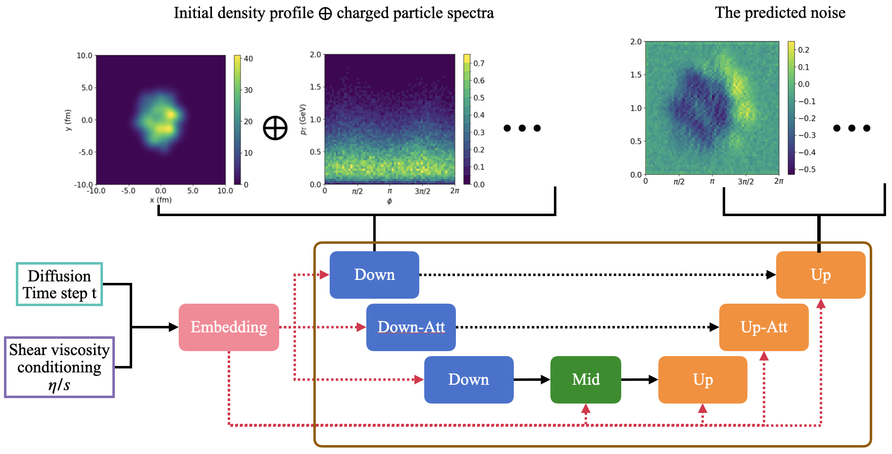
The conditional reverse diffusion process is accomplished by learning the scaled score function through a noise-prediction network as depicted in the workflow shown in Figure 1. The initial density profiles and corresponding particle spectra are concatenated channel-wise. The diffusion time steps and are encoded via a time-embedding and label-embedding layer, respectively, which are further added together. The input charged particle spectra are noised according to . A noise-prediction network are used, aiming to minimize the mean squared error . The training algorithm is summarized in Algorithm 1. Once we have a such trained scaled score function , the particle spectra can be generated from Gaussian noise by solving the reverse ODE (Eq. 5). In this model, the total noise steps is and we chose a linear noise schedule from to .
Model Performance.— To evaluate the performance of our trained DiffHIC model, we conducted additional 10,000-event simulations for each value of across all centralities. We assess the efficacy of DiffHIC by comparing its outputs with the original numerical simulations, which were regarded as the ground truth. In terms of the generated particle spectrum, which in practice is a two-dimensional discretized distribution of pixels of size (in and ), perfect comparison between DIffHIC and the ground truth is realized with impurities appear only randomly at a level of several pixels.
Below we primarily focus on the anisotropic flow, as they are measurables that quantitatively characterize the spectrum. Anisotropic flow are defined as the Fourier coefficients of the particle spectrum,
with the event plane angle. These flow signatures depend on harmonic order , as well as transverse momentum. Note that the mean transverse momentum, , can be deduced from .
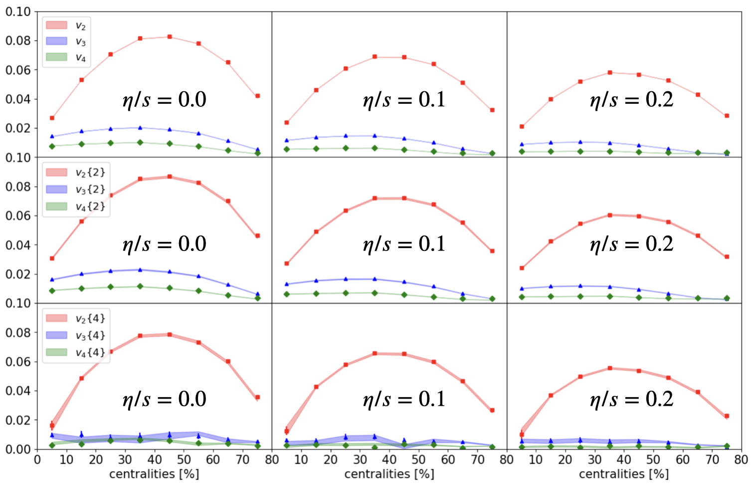
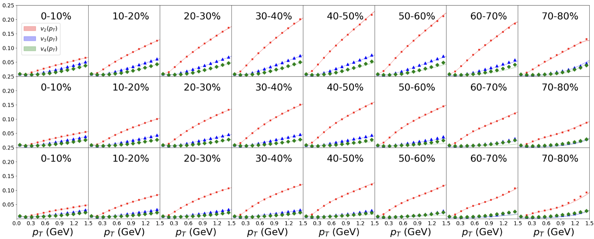
Comparisons involving other observables, including in particular correlations and fluctuations among these flow observables [1, 2, 76, 33, 26, 77, 78, 79], are detailed in the Supplemental Material. We first present here the integrated flow and differential flow. Owing to event-by-event fluctuations, anisotropic flow can be measured with respect to an event plane, or from multi-particle cumulants. In Fig. 2, the integrated flow of order are shown for all centralities, from the event-plane method (top panels), and two-particle cumulant (middle panels) and four-particle cumulant (bottom panels). Comparing to the ground truth (filled symbols), DiffHIC (colored bands) reproduces in general the predictions of the integrated flow, with slight deviation visible for in the four-particle cumulant. The deviation gets reduced as increases. Although differential flow signatures are normally more demanding for model characterizations, in Fig. 3, one observes a perfect comparison between the ground truth (filled symbols) and the DiffHIC predictions (colored bands) for the -dependent anisotropic flow, through all centralities.
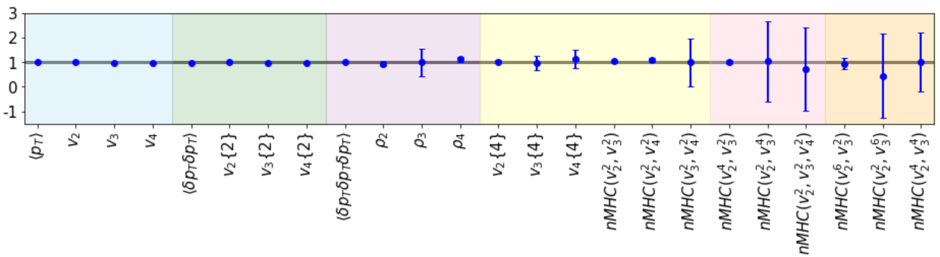
To explicitly demonstrate the performance of DiffHIC, the ratios of observables, comparing the generative model to traditional simulations, are shown in Fig. 4. From left to right, the number of particle correlations involved increases, as indicated by the different color regions. These ratios are close to unity, indicating the validity of DiffHIC. Although the model precision decreases systematically as the number of correlated particles increases, it is to some extent anticipated since our simulations are limited by the spectrum resolution of . A higher-resolution model would capture more details of the heavy-ion dynamics. Similar issues also exist in the high- region and peripheral collisions, where effective pixels of the spectrum reduce significantly. Another limitation is the model may struggle in other systems with different collision energies, especially for high-order fluctuations and correlations. Nonetheless, improvement should be achieved by training a model with better resolution. Given the efficiency and flexibility of DiffHIC, fine-tuning our trained model in the new dataset or retraining a specific model is also a possible solution.
Conclusions and Outlook.— In this Letter, the state-of-art generative model (DiffHIC) is for the first time trained to generate the final particle spectra, from event-by-event initial entropy density profiles. While being capable of capturing the two-dimensional distribution in the momentum space accurately, as an end-to-end model, DiffHIC speeds up the numerical simulations by a factor of roughly , compared to the traditional approach. Consequently, DiffHIC alleviates time and resource concerns. The DifHIC model aims to be applicable to high-precision experimental measurements, establishing a solid theoretical foundation for interpreting observables based on a huge amount of collision data, particularly in relation to the fine structures present in the systems. These include features such as nuclear deformation and the equation of state in the QGP.
Acknowledgements.— Jing-An Sun thanks Xiangyu Wu, Lipei Du, and Han Gao for helpful discussions. This work is funded in part by the Natural Sciences and Engineering Research Council of Canada (NSERC) [SAPIN-2020-00048 and SAPIN-2024-00026], in part by the China Scholarship Council, and in part by the National Natural Science Foundation of China under Grants No. 12375133 and 12147101. The dataset preparations are made on the Beluga supercomputer system at McGill University, managed by Calcul Quebec and the Digital Research Alliance of Canada. The operation of this supercomputer is funded by the Canada Foundation for Innovation (CFI), Ministère de l’Économie, des Sciences et de l’Innovation du Québec (MESI) and le Fonds de recherche du Québec - Nature et technologies (FRQ-NT).
References
- Shuryak [2017] E. Shuryak, Strongly coupled quark-gluon plasma in heavy ion collisions, Rev. Mod. Phys. 89, 035001 (2017), arXiv:1412.8393 [hep-ph] .
- Heinz and Snellings [2013] U. Heinz and R. Snellings, Collective flow and viscosity in relativistic heavy-ion collisions, Ann. Rev. Nucl. Part. Sci. 63, 123 (2013), arXiv:1301.2826 [nucl-th] .
- Bass and Dumitru [2000] S. A. Bass and A. Dumitru, Dynamics of hot bulk QCD matter: From the quark gluon plasma to hadronic freezeout, Phys. Rev. C 61, 064909 (2000), arXiv:nucl-th/0001033 .
- Hirano et al. [2008] T. Hirano, U. W. Heinz, D. Kharzeev, R. Lacey, and Y. Nara, Mass ordering of differential elliptic flow and its violation for phi mesons, Phys. Rev. C 77, 044909 (2008), arXiv:0710.5795 [nucl-th] .
- Nonaka and Bass [2007] C. Nonaka and S. A. Bass, Space-time evolution of bulk QCD matter, Phys. Rev. C 75, 014902 (2007), arXiv:nucl-th/0607018 .
- Petersen et al. [2008a] H. Petersen, J. Steinheimer, G. Burau, M. Bleicher, and H. Stöcker, A Fully Integrated Transport Approach to Heavy Ion Reactions with an Intermediate Hydrodynamic Stage, Phys. Rev. C 78, 044901 (2008a), arXiv:0806.1695 [nucl-th] .
- Ryu et al. [2018] S. Ryu, J.-F. Paquet, C. Shen, G. Denicol, B. Schenke, S. Jeon, and C. Gale, Effects of bulk viscosity and hadronic rescattering in heavy ion collisions at energies available at the BNL Relativistic Heavy Ion Collider and at the CERN Large Hadron Collider, Phys. Rev. C 97, 034910 (2018), arXiv:1704.04216 [nucl-th] .
- Song et al. [2011] H. Song, S. A. Bass, and U. Heinz, Viscous QCD matter in a hybrid hydrodynamic+Boltzmann approach, Phys. Rev. C 83, 024912 (2011), arXiv:1012.0555 [nucl-th] .
- Zhu et al. [2015] X. Zhu, F. Meng, H. Song, and Y.-X. Liu, Hybrid model approach for strange and multistrange hadrons in 2.76A TeV Pb+Pb collisions, Phys. Rev. C 91, 034904 (2015), arXiv:1501.03286 [nucl-th] .
- Yan [2018] L. Yan, A flow paradigm in heavy-ion collisions, Chin. Phys. C 42, 042001 (2018), arXiv:1712.04580 [nucl-th] .
- Shen and Yan [2020] C. Shen and L. Yan, Recent development of hydrodynamic modeling in heavy-ion collisions, Nucl. Sci. Tech. 31, 122 (2020), arXiv:2010.12377 [nucl-th] .
- Vredevoogd and Pratt [2009] J. Vredevoogd and S. Pratt, Universal Flow in the First Stage of Relativistic Heavy Ion Collisions, Phys. Rev. C 79, 044915 (2009), arXiv:0810.4325 [nucl-th] .
- Mueller and Schaefer [2011] B. Mueller and A. Schaefer, Entropy creation in relativistic heavy ion collisions, International Journal of Modern Physics E 20, 2235 (2011).
- Schenke et al. [2012] B. Schenke, P. Tribedy, and R. Venugopalan, Fluctuating Glasma initial conditions and flow in heavy ion collisions, Phys. Rev. Lett. 108, 252301 (2012), arXiv:1202.6646 [nucl-th] .
- van der Schee et al. [2013] W. van der Schee, P. Romatschke, and S. Pratt, Fully Dynamical Simulation of Central Nuclear Collisions, Phys. Rev. Lett. 111, 222302 (2013), arXiv:1307.2539 [nucl-th] .
- Berges et al. [2014] J. Berges, B. Schenke, S. Schlichting, and R. Venugopalan, Turbulent thermalization process in high-energy heavy-ion collisions, Nucl. Phys. A 931, 348 (2014), arXiv:1409.1638 [hep-ph] .
- Kurkela and Lu [2014] A. Kurkela and E. Lu, Approach to Equilibrium in Weakly Coupled Non-Abelian Plasmas, Phys. Rev. Lett. 113, 182301 (2014), arXiv:1405.6318 [hep-ph] .
- Kurkela et al. [2019a] A. Kurkela, A. Mazeliauskas, J.-F. Paquet, S. Schlichting, and D. Teaney, Effective kinetic description of event-by-event pre-equilibrium dynamics in high-energy heavy-ion collisions, Phys. Rev. C 99, 034910 (2019a), arXiv:1805.00961 [hep-ph] .
- Kurkela et al. [2020] A. Kurkela, W. van der Schee, U. A. Wiedemann, and B. Wu, Early- and Late-Time Behavior of Attractors in Heavy-Ion Collisions, Phys. Rev. Lett. 124, 102301 (2020), arXiv:1907.08101 [hep-ph] .
- Kurkela et al. [2019b] A. Kurkela, A. Mazeliauskas, J.-F. Paquet, S. Schlichting, and D. Teaney, Matching the Nonequilibrium Initial Stage of Heavy Ion Collisions to Hydrodynamics with QCD Kinetic Theory, Phys. Rev. Lett. 122, 122302 (2019b), arXiv:1805.01604 [hep-ph] .
- Schlichting and Teaney [2019] S. Schlichting and D. Teaney, The First fm/c of Heavy-Ion Collisions, Ann. Rev. Nucl. Part. Sci. 69, 447 (2019), arXiv:1908.02113 [nucl-th] .
- Schenke et al. [2011] B. Schenke, S. Jeon, and C. Gale, Elliptic and triangular flow in event-by-event (3+1)D viscous hydrodynamics, Phys. Rev. Lett. 106, 042301 (2011), arXiv:1009.3244 [hep-ph] .
- Schenke et al. [2010] B. Schenke, S. Jeon, and C. Gale, (3+1)D hydrodynamic simulation of relativistic heavy-ion collisions, Phys. Rev. C 82, 014903 (2010), arXiv:1004.1408 [hep-ph] .
- Paquet et al. [2016] J.-F. Paquet, C. Shen, G. S. Denicol, M. Luzum, B. Schenke, S. Jeon, and C. Gale, Production of photons in relativistic heavy-ion collisions, Phys. Rev. C 93, 044906 (2016), arXiv:1509.06738 [hep-ph] .
- Gale et al. [2022] C. Gale, J.-F. Paquet, B. Schenke, and C. Shen, Multimessenger heavy-ion collision physics, Phys. Rev. C 105, 014909 (2022), arXiv:2106.11216 [nucl-th] .
- Romatschke [2010] P. Romatschke, New Developments in Relativistic Viscous Hydrodynamics, Int. J. Mod. Phys. E 19, 1 (2010), arXiv:0902.3663 [hep-ph] .
- Florkowski et al. [2018] W. Florkowski, M. P. Heller, and M. Spalinski, New theories of relativistic hydrodynamics in the LHC era, Rept. Prog. Phys. 81, 046001 (2018), arXiv:1707.02282 [hep-ph] .
- Gale et al. [2013] C. Gale, S. Jeon, and B. Schenke, Hydrodynamic Modeling of Heavy-Ion Collisions, Int. J. Mod. Phys. A 28, 1340011 (2013), arXiv:1301.5893 [nucl-th] .
- Weil et al. [2016] J. Weil et al. (SMASH), Particle production and equilibrium properties within a new hadron transport approach for heavy-ion collisions, Phys. Rev. C 94, 054905 (2016), arXiv:1606.06642 [nucl-th] .
- Bass et al. [1998] S. A. Bass et al., Microscopic models for ultrarelativistic heavy ion collisions, Prog. Part. Nucl. Phys. 41, 255 (1998), arXiv:nucl-th/9803035 .
- Bleicher et al. [1999] M. Bleicher et al., Relativistic hadron hadron collisions in the ultrarelativistic quantum molecular dynamics model, J. Phys. G 25, 1859 (1999), arXiv:hep-ph/9909407 .
- Petersen et al. [2008b] H. Petersen, J. Steinheimer, G. Burau, M. Bleicher, and H. Stöcker, A Fully Integrated Transport Approach to Heavy Ion Reactions with an Intermediate Hydrodynamic Stage, Phys. Rev. C 78, 044901 (2008b), arXiv:0806.1695 [nucl-th] .
- Ollitrault [1992] J.-Y. Ollitrault, Anisotropy as a signature of transverse collective flow, Phys. Rev. D 46, 229 (1992).
- Arslandok et al. [2023] M. Arslandok et al., Hot QCD White Paper (2023), arXiv:2303.17254 [nucl-ex] .
- Acharya et al. [2024] S. Acharya et al. (ALICE), The ALICE experiment: a journey through QCD, Eur. Phys. J. C 84, 813 (2024), arXiv:2211.04384 [nucl-ex] .
- Fortier et al. [2023] N. Fortier, S. Jeon, and C. Gale, Comparisons and Predictions for Collisions of deformed 238U nuclei at GeV (2023), arXiv:2308.09816 [nucl-th] .
- Jia et al. [2022] J. Jia, S. Huang, and C. Zhang, Probing nuclear quadrupole deformation from correlation of elliptic flow and transverse momentum in heavy ion collisions, Phys. Rev. C 105, 014906 (2022), arXiv:2105.05713 [nucl-th] .
- Bally et al. [2022] B. Bally, M. Bender, G. Giacalone, and V. Somà, Evidence of the triaxial structure of 129Xe at the Large Hadron Collider, Phys. Rev. Lett. 128, 082301 (2022), arXiv:2108.09578 [nucl-th] .
- Bozek [2016] P. Bozek, Transverse-momentum–flow correlations in relativistic heavy-ion collisions, Phys. Rev. C 93, 044908 (2016), arXiv:1601.04513 [nucl-th] .
- Gardim et al. [2020] F. G. Gardim, G. Giacalone, and J.-Y. Ollitrault, The mean transverse momentum of ultracentral heavy-ion collisions: A new probe of hydrodynamics, Phys. Lett. B 809, 135749 (2020), arXiv:1909.11609 [nucl-th] .
- Sun and Yan [2024] J.-A. Sun and L. Yan, Volume effect on the extraction of sound velocity in high-energy nucleus-nucleus collisions (2024), arXiv:2407.05570 [nucl-th] .
- Hayrapetyan et al. [2024] A. Hayrapetyan et al. (CMS), Extracting the speed of sound in the strongly interacting matter created in ultrarelativistic lead-lead collisions at the LHC (2024), arXiv:2401.06896 [nucl-ex] .
- Nijs and van der Schee [2024] G. Nijs and W. van der Schee, Ultracentral heavy ion collisions, transverse momentum and the equation of state, Phys. Lett. B 853, 138636 (2024), arXiv:2312.04623 [nucl-th] .
- Heffernan et al. [2024] M. R. Heffernan, C. Gale, S. Jeon, and J.-F. Paquet, Early-Times Yang-Mills Dynamics and the Characterization of Strongly Interacting Matter with Statistical Learning, Phys. Rev. Lett. 132, 252301 (2024), arXiv:2306.09619 [nucl-th] .
- Huang et al. [2021a] H. Huang, B. Xiao, Z. Liu, Z. Wu, Y. Mu, and H. Song, Applications of deep learning to relativistic hydrodynamics, Phys. Rev. Res. 3, 023256 (2021a), arXiv:1801.03334 [nucl-th] .
- Liyanage et al. [2022] D. Liyanage, Y. Ji, D. Everett, M. Heffernan, U. Heinz, S. Mak, and J.-F. Paquet, Efficient emulation of relativistic heavy ion collisions with transfer learning, Phys. Rev. C 105, 034910 (2022), arXiv:2201.07302 [nucl-th] .
- Ho et al. [2020] J. Ho, A. Jain, and P. Abbeel, Denoising diffusion probabilistic models, in Proceedings of the 34th International Conference on Neural Information Processing Systems, NIPS ’20 (Curran Associates Inc., Red Hook, NY, USA, 2020).
- Sohl-Dickstein et al. [2015] J. Sohl-Dickstein, E. Weiss, N. Maheswaranathan, and S. Ganguli, Deep unsupervised learning using nonequilibrium thermodynamics, in International conference on machine learning (PMLR, 2015) pp. 2256–2265.
- Song et al. [2021a] Y. Song, J. Sohl-Dickstein, D. P. Kingma, A. Kumar, S. Ermon, and B. Poole, Score-based generative modeling through stochastic differential equations, in International Conference on Learning Representations (2021).
- Dhariwal and Nichol [2024] P. Dhariwal and A. Nichol, Diffusion models beat gans on image synthesis, in Proceedings of the 35th International Conference on Neural Information Processing Systems, NIPS ’21 (Curran Associates Inc., Red Hook, NY, USA, 2024).
- Ho et al. [2022] J. Ho, C. Saharia, W. Chan, D. J. Fleet, M. Norouzi, and T. Salimans, Cascaded diffusion models for high fidelity image generation, Journal of Machine Learning Research 23, 1 (2022).
- Song et al. [2021b] Y. Song, C. Durkan, I. Murray, and S. Ermon, Maximum likelihood training of score-based diffusion models, Advances in neural information processing systems 34, 1415 (2021b).
- Huang et al. [2021b] C.-W. Huang, J. H. Lim, and A. C. Courville, A variational perspective on diffusion-based generative models and score matching, Advances in Neural Information Processing Systems 34, 22863 (2021b).
- Kingma et al. [2021] D. Kingma, T. Salimans, B. Poole, and J. Ho, Variational diffusion models, Advances in neural information processing systems 34, 21696 (2021).
- Amram and Pedro [2023] O. Amram and K. Pedro, Denoising diffusion models with geometry adaptation for high fidelity calorimeter simulation, Phys. Rev. D 108, 072014 (2023), arXiv:2308.03876 [physics.ins-det] .
- Go et al. [2024] Y. Go, D. Torbunov, T. Rinn, Y. Huang, H. Yu, B. Viren, M. Lin, Y. Ren, and J. Huang, Effectiveness of denoising diffusion probabilistic models for fast and high-fidelity whole-event simulation in high-energy heavy-ion experiments (2024), arXiv:2406.01602 [physics.data-an] .
- Leigh et al. [2024a] M. Leigh, D. Sengupta, G. Quétant, J. A. Raine, K. Zoch, and T. Golling, PC-JeDi: Diffusion for particle cloud generation in high energy physics, SciPost Phys. 16, 018 (2024a), arXiv:2303.05376 [hep-ph] .
- Leigh et al. [2024b] M. Leigh, D. Sengupta, J. A. Raine, G. Quétant, and T. Golling, Faster diffusion model with improved quality for particle cloud generation, Phys. Rev. D 109, 012010 (2024b), arXiv:2307.06836 [hep-ex] .
- Mikuni et al. [2023] V. Mikuni, B. Nachman, and M. Pettee, Fast point cloud generation with diffusion models in high energy physics, Phys. Rev. D 108, 036025 (2023), arXiv:2304.01266 [hep-ph] .
- Mikuni and Nachman [2024] V. Mikuni and B. Nachman, CaloScore v2: single-shot calorimeter shower simulation with diffusion models, JINST 19 (02), P02001, arXiv:2308.03847 [hep-ph] .
- Shmakov et al. [2023] A. Shmakov, K. Greif, M. Fenton, A. Ghosh, P. Baldi, and D. Whiteson, End-to-end latent variational diffusion models for inverse problems in high energy physics (2023), arXiv:2305.10399 [hep-ex] .
- He et al. [2023] W.-B. He, Y.-G. Ma, L.-G. Pang, H.-C. Song, and K. Zhou, High-energy nuclear physics meets machine learning, Nucl. Sci. Tech. 34, 88 (2023), arXiv:2303.06752 [hep-ph] .
- Ma et al. [2023] Y.-G. Ma, L.-G. Pang, R. Wang, and K. Zhou, Phase Transition Study Meets Machine Learning, Chin. Phys. Lett. 40, 122101 (2023), arXiv:2311.07274 [nucl-th] .
- Pang [2024] L.-G. Pang, Studying high-energy nuclear physics with machine learning, Int. J. Mod. Phys. E 33, 2430009 (2024).
- Zhou et al. [2024] K. Zhou, L. Wang, L.-G. Pang, and S. Shi, Exploring QCD matter in extreme conditions with Machine Learning, Prog. Part. Nucl. Phys. 135, 104084 (2024), arXiv:2303.15136 [hep-ph] .
- Anderson [1982] B. D. Anderson, Reverse-time diffusion equation models, Stochastic Processes and their Applications 12, 313 (1982).
- Vincent [2011] P. Vincent, A connection between score matching and denoising autoencoders, Neural Computation 23, 1661 (2011).
- Zheng et al. [2023] K. Zheng, C. Lu, J. Chen, and J. Zhu, Dpm-solver-v3: Improved diffusion ode solver with empirical model statistics, in Thirty-seventh Conference on Neural Information Processing Systems (2023).
- Lu et al. [2022] C. Lu, Y. Zhou, F. Bao, J. Chen, C. Li, and J. Zhu, DPM-solver: A fast ODE solver for diffusion probabilistic model sampling in around 10 steps, in Advances in Neural Information Processing Systems, edited by A. H. Oh, A. Agarwal, D. Belgrave, and K. Cho (2022).
- Lu et al. [2023] C. Lu, Y. Zhou, F. Bao, J. Chen, C. Li, and J. Zhu, Dpm-solver++: Fast solver for guided sampling of diffusion probabilistic models (2023), arXiv:2211.01095 [cs.LG] .
- Moreland et al. [2015] J. S. Moreland, J. E. Bernhard, and S. A. Bass, Alternative ansatz to wounded nucleon and binary collision scaling in high-energy nuclear collisions, Phys. Rev. C 92, 011901 (2015), arXiv:1412.4708 [nucl-th] .
- Cooper and Frye [1974] F. Cooper and G. Frye, Comment on the Single Particle Distribution in the Hydrodynamic and Statistical Thermodynamic Models of Multiparticle Production, Phys. Rev. D 10, 186 (1974).
- Huovinen and Petersen [2012] P. Huovinen and H. Petersen, Particlization in hybrid models, Eur. Phys. J. A 48, 171 (2012), arXiv:1206.3371 [nucl-th] .
- He et al. [2016] K. He, X. Zhang, S. Ren, and J. Sun, Deep residual learning for image recognition, in 2016 IEEE Conference on Computer Vision and Pattern Recognition (CVPR) (2016) pp. 770–778.
- Vaswani et al. [2017] A. Vaswani, N. Shazeer, N. Parmar, J. Uszkoreit, L. Jones, A. N. Gomez, L. Kaiser, and I. Polosukhin, Attention is all you need, in Proceedings of the 31st International Conference on Neural Information Processing Systems, NIPS’17 (Curran Associates Inc., Red Hook, NY, USA, 2017) p. 6000–6010.
- Alver and Roland [2010] B. Alver and G. Roland, Collision geometry fluctuations and triangular flow in heavy-ion collisions, Phys. Rev. C 81, 054905 (2010), [Erratum: Phys.Rev.C 82, 039903 (2010)], arXiv:1003.0194 [nucl-th] .
- Teaney and Yan [2011] D. Teaney and L. Yan, Triangularity and Dipole Asymmetry in Heavy Ion Collisions, Phys. Rev. C 83, 064904 (2011), arXiv:1010.1876 [nucl-th] .
- Teaney and Yan [2012] D. Teaney and L. Yan, Non linearities in the harmonic spectrum of heavy ion collisions with ideal and viscous hydrodynamics, Phys. Rev. C 86, 044908 (2012), arXiv:1206.1905 [nucl-th] .
- Yan and Ollitrault [2014] L. Yan and J.-Y. Ollitrault, Universal fluctuation-driven eccentricities in proton-proton, proton-nucleus and nucleus-nucleus collisions, Phys. Rev. Lett. 112, 082301 (2014), arXiv:1312.6555 [nucl-th] .
- Li et al. [2021] M. Li, Y. Zhou, W. Zhao, B. Fu, Y. Mou, and H. Song, Investigations on mixed harmonic cumulants in heavy-ion collisions at energies available at the CERN Large Hadron Collider, Phys. Rev. C 104, 024903 (2021), arXiv:2104.10422 [nucl-th] .
- Adam et al. [2016] J. Adam et al. (ALICE), Correlated event-by-event fluctuations of flow harmonics in Pb-Pb collisions at TeV, Phys. Rev. Lett. 117, 182301 (2016), arXiv:1604.07663 [nucl-ex] .
- Acharya et al. [2018] S. Acharya et al. (ALICE), Systematic studies of correlations between different order flow harmonics in Pb-Pb collisions at = 2.76 TeV, Phys. Rev. C 97, 024906 (2018), arXiv:1709.01127 [nucl-ex] .
- Bhatta et al. [2022] S. Bhatta, C. Zhang, and J. Jia, Higher-order transverse momentum fluctuations in heavy-ion collisions, Phys. Rev. C 105, 024904 (2022), arXiv:2112.03397 [nucl-th] .
- Giacalone et al. [2021] G. Giacalone, F. G. Gardim, J. Noronha-Hostler, and J.-Y. Ollitrault, Skewness of mean transverse momentum fluctuations in heavy-ion collisions, Phys. Rev. C 103, 024910 (2021), arXiv:2004.09799 [nucl-th] .
- Schenke et al. [2020] B. Schenke, C. Shen, and D. Teaney, Transverse momentum fluctuations and their correlation with elliptic flow in nuclear collision, Phys. Rev. C 102, 034905 (2020), arXiv:2004.00690 [nucl-th] .
Appendix A supplemental material
A.1 The model parameters used when preparing the datasets
Initial Stage:
We choose the most probable values from the Bayesian analysis, . The norm factors are set to for PbPb@5.02TeV. The grid size is and
Hydrodynamic Stage:
We turn off the bulk viscosity during the evolution. The initial time is 0.4 fm. The freezeout energy density is chosen at 0.18 GeV/fm3. To view the effect of the shear viscosity, we run simulations at three different values, . The effect of bulk viscosity is neglected.
Particlization and afterburner:
The default parameters in UrQMD are used.
A.2 The charged particle spectra
In momentum space, the azimuthal emitted particle distribution can be written as
| (6) |
where is the -th order anisotropic flow coefficient and is its corresponding flow plane angle. Both are differential. One can also perform Fourier expansion for the integrated spectra,
| (7) |
where is the -th order integrated anisotropic flow and is its corresponding flow plane angle.
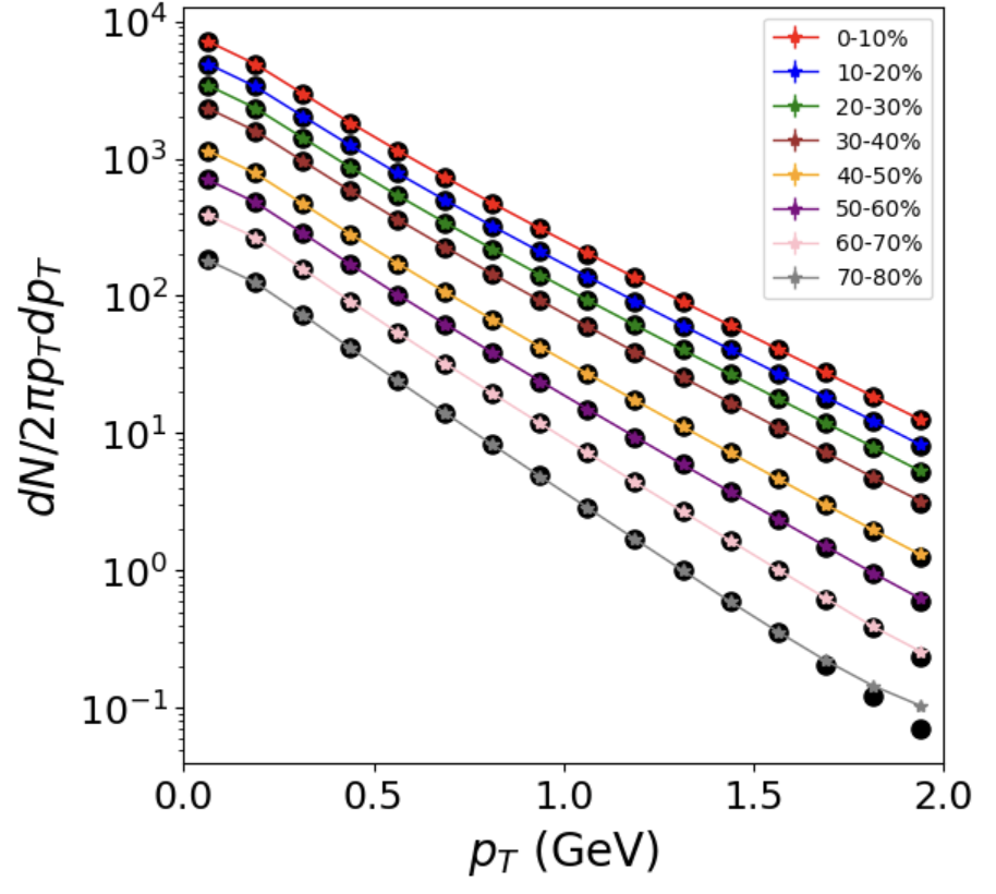
We present charged particle transverse momentum spectra across all centralities in Fig. 5. It is shown that the model predictions (color lines) perfectly agree with the ground truth ( black circles).
A.3 Mixed harmonic coeffients
The mixed harmonic coefficients (MHC) have been proposed to quantify the correlation strength between different orders of flow coefficients and various moments, as they are expected to be more sensitive to medium properties and initial state correlations [80, 81, 82]. Additionally, MHC excludes symmetry plane correlations, making it less sensitive to non-flow contaminations.
The 4-particle mixed harmonic cumulants (MHC) are defined as,
| (8) |
The 6-particle cumulants are defined as,
The 8-particle cumulants are defined as,
To eliminate the flow magnitude effect, the normalized cumulants can be used.
| (9) | ||||
| (10) |
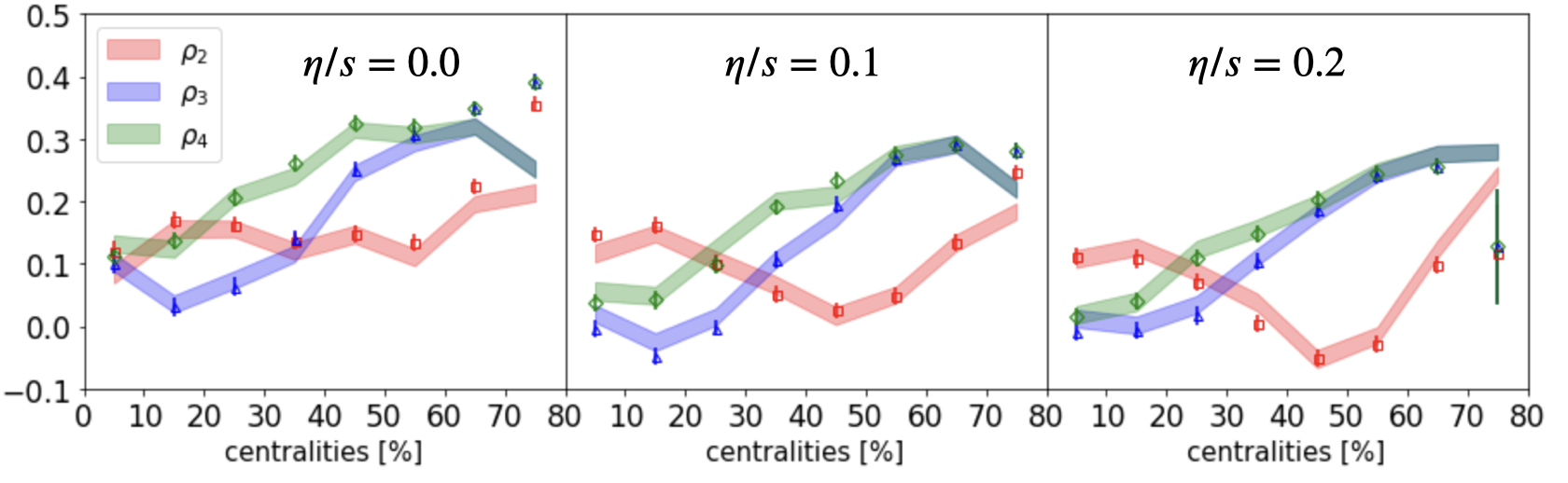
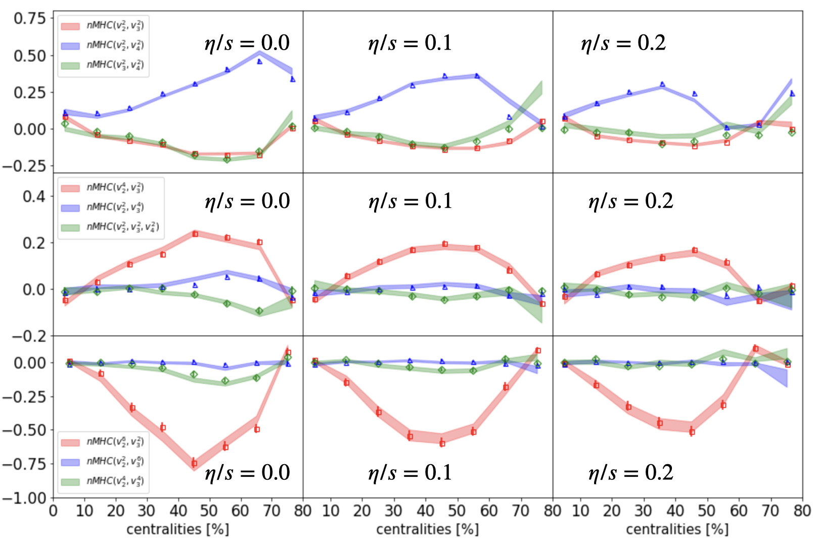
In Fig. 6, we compare the ground truth and the generated results for various flow correlations. Except for the correlation at the very last peripheral bin, the agreements are excellent.
A.4 The mean transverse momentum correlations
The event-by-event mean transverse momentum fluctuations are other probes, which are sensitive to initial state fluctuations [83, 36, 84].
The second and third-order correlators are defined as,
| (11) | ||||
| (12) |
In a single event, is the transverse momentum of th particle. is the total number of charged particles. is the event-averaged mean transverse momentum. For efficient computations, in each event, we define
| (13) |
The and sums over pairs and triplets of particles can be expressed simply in terms of ():
| (14) | ||||
| (15) | ||||
| (16) |
Thus, the correlators can be simplified as,
| (17) | ||||
| (18) |
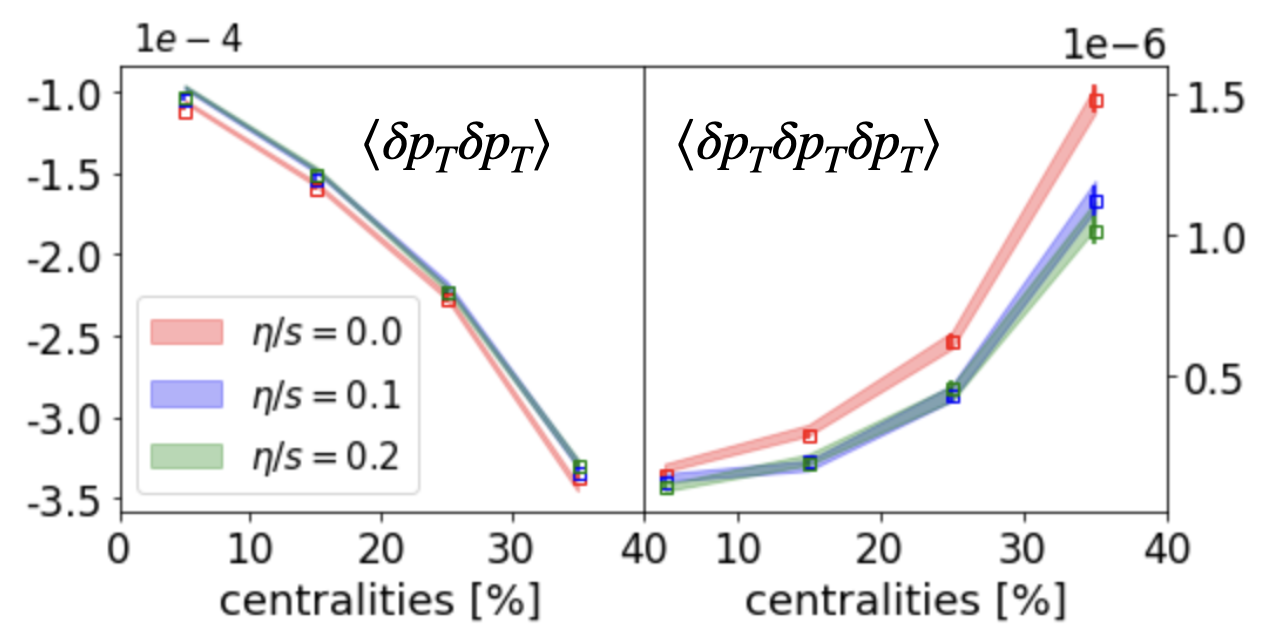
Fig.7 presents the centrality dependence of (left panel) and (right panel). The trained model calculations are highly consistent with the numerical simulations implying that the underlying energy density fluctuations and flow velocity fluctuations are well captured by the model.
A.5 The flow and transverse momentum correlations
In the past few years, the correlations between flow and mean transverse momentum have been put forward to infer the nuclear shape [37, 38, 39, 85]. It can be calculated as,
| (19) |
where are the standard variance of and , respectively. Fig. 8 shows that the ground truth and the generated results are in good agreement except for the very last peripheral bin where hydrodynamics may not fully apply.