Systems with Switching Causal Relations:
A Meta-Causal Perspective

Abstract

Most work on causality in machine learning assumes that causal relationships are driven by a constant underlying process. However, the flexibility of agents’ actions or tipping points in the environmental process can change the qualitative dynamics of the system. As a result, new causal relationships may emerge, while existing ones change or disappear, resulting in an altered causal graph. To analyze these qualitative changes on the causal graph, we propose the concept of meta-causal states, which groups classical causal models into clusters based on equivalent qualitative behavior and consolidates specific mechanism parameterizations. We demonstrate how meta-causal states can be inferred from observed agent behavior, and discuss potential methods for disentangling these states from unlabeled data. Finally, we direct our analysis towards the application of a dynamical system, showing that meta-causal states can also emerge from inherent system dynamics, and thus constitute more than a context-dependent framework in which mechanisms emerge only as a result of external factors.

1 Introduction

Structural Causal Models (SCM) have become the de facto formalism in causality by representing causal relations a structural equation models (Pearl (2009); Spirtes et al. (2000)). While SCM are most useful for representing the intricate mechanistic details of systems, it can be challenging to derive the general qualitative behavior that emerges from the interplay of individual equations. Talking about the general type of relation emitted by particular mechanisms generalizes above the narrow computational view and has the ability to inspect causal systems from a more general perspective. Causal graphs can be subject to change whenever novel mechanisms emerge or vanish within a system. Prominently, agents can ‘break’ the natural unfolding of systems dynamics by forecasting system behavior and preemptively intervening in the course of events. As inherent parts of the environment, agents commonly establish or suppress the emergence of causal connections (Zhang & Bareinboim, 2017; Lee & Bareinboim, 2018; Dasgupta et al., 2019).

Consider the scenario shown in Fig. 1 (left), where an agent $A$ (with position $A_{X}$) follows an agent $B$ (with position $B_{X}$) according to its policy $A_{\operatorname{\bm{\pi}}}$. We are interested in answering the question ‘What is the cause of the current position of agent A?’. In general, the observed system can be formalized as follows: $A_{X}:=f_{A}(B_{X},U_{A})$ and $B_{X}:=f_{B}(U_{B})$. From a classical causal perspective we observe that $B\rightarrow A$, since $A_{X}$ is conditioned on $B_{X}$ via the equation $f_{A}$. As a result, we infer that $B_{X}$ is the cause of $A$’s position. This perspective, only attributes causes within the current state of the system. However, it disregards the causes that lead to the emergence of $f_{A}$. Only when we take a meta-causal stance and think about how the equation $f_{A}$ came to be in the first place, we can give the answer that $A$, through its policy $A_{\operatorname{\bm{\pi}}}$, is the (meta-causal) cause for its own position.

Causal models do not exist in isolation, but emerge from the environmental dynamics of an underlying mediation process (Hofmann et al., 2020; Arnellos et al., 2006). Changes in causal relations due to intervention or environmental change are often assumed to be helpful conditions for identifying causal structures (Pearl, 2009; Peters et al., 2016; Zhang & Bareinboim, 2017; Dasgupta et al., 2019; Gerstenberg, 2024). These operations often work on the individual causal graphs, but never reason about the emerging meta-causal structure that governs the transitions between the different SCM. As a first formalization of metacausal models in this area, we describe how qualitative changes in the causal graphs can be summarized by metacausal models.

    

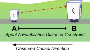
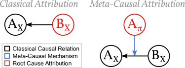
Figure 1: Meta-Causality Identifies the Policy as a Meta Root Cause. Agent $A$ intends to maintain its distance from agent $B$ by conditioning its position $A_{X}$ on the position $B_{X}$, which establishes a control mechanism, $A_{X}:=f(B_{X})$. In standard causal inference, we would infer $B_{X}\rightarrow A_{X}$ and, therefore, $B$ to be the root cause. Taking a meta-causal perspective reveals however, that $A_{\operatorname{\bm{\pi}}}$ establishes the edge $B_{X}\rightarrow A_{X}$ in the first place ($\text{$A_{\operatorname{\bm{\pi}}}$}\rightarrow\text{($B_{X}\rightarrow A_{X}$)}$) such that $A_{\operatorname{\bm{\pi}}}$ is considered the root cause on the meta-level. (Best Viewed in Color)

Contributions and Structure. The contributions of this work are as follows:

• To the best of our knowledge, we are the first to formally introduce typing mechanisms that generalize edges in causal graphs, and the first to provide a formalization of meta-causal models (MCM) that are capable of capturing the switching type dynamics of causal mechanisms.

• We present an approach to discover the number of meta-causal states in the bivariate case.

• We demonstrate that meta-causal models can be more powerful than classical SCM when it comes to expressing qualitative differences within certain system dynamics.

• We show how meta-causal analysis can lead to a different root cause attribution than classical causal inference, and is furthermore able to identify causes of mechanistic changes even when no actual change in effect can be observed.

We proceed as follows: In Section 2 we describe the necessary basics of Pearlian causality, mediation processes, and typing assumptions. In Sec. 3 we introduce meta-causality by first formalizing meta-causal frames, and the role of types as a generalization to a binary edge representations. Finally we define meta-causal models that are able to capture the qualitative dynamics in SCM behavior. In Sec. 4, we showcase several examples of meta-causal applications. Finally, we discuss connections to related work in Sec. 5 and conclude our findings in Sec. 6.

2 Background

Providing a higher-level perspective on meta-causality touches on a number of existing works that leverage meta-causal ideas, even if not explicitly stated. We will highlight relations of these works in the ‘Related Work’ of section 5. Here, we continue to provide the necessary concepts on causality, mediation processes and typing, needed for the definitions in our paper:

Causal Models. A common formalization of causality is provided via Structural Causal Models (SCM; (Spirtes et al., 2000; Pearl, 2009)). An SCM is defined as a tuple $\operatorname{\mathcal{M}}:=(\operatorname{\mathbf{U}},\operatorname{\mathbf{V}},\operatorname{\mathbf{F}},P_{\operatorname{\mathbf{U}}})$, where $\operatorname{\mathbf{U}}$ is the set of exogenous variables, $\operatorname{\mathbf{V}}$ is the set of endogenous variables, $\operatorname{\mathbf{F}}$ is the set of structural equations determining endogenous variables, and $P_{\operatorname{\mathbf{U}}}$ is the distribution over exogenous variables $\operatorname{\mathbf{U}}$. Every endogenous variable $V_{i}\in\operatorname{\mathbf{V}}$ is determined via a structural equation $v_{i}:=f_{i}(\text{pa}(v_{i}))$ that takes in a set of parent values $\text{pa}(v_{i})$, consisting of endogenous and exogenous variables, and outputs the value of $v_{i}$. The set of all variables is denoted by $\operatorname{\mathbf{X}}=\operatorname{\mathbf{U}}\cup\operatorname{\mathbf{V}}$ with values $\mathbf{x}\in\operatorname{\bm{\mathcal{X}}}$ and $N=|\operatorname{\mathbf{X}}|$. Every SCM $\operatorname{\mathcal{M}}$ entails a directed graph $\mathcal{G}^{\operatorname{\mathcal{M}}}$ that can be constructed by adding edges $(i,j)\in\operatorname{\mathbf{X}}\times\operatorname{\mathbf{X}}$ for all variables $X_{j}\in\operatorname{\mathbf{X}}$ and its parents $X_{i}\in\text{Pa}(X_{j})$. This can be expressed as an adjacency matrix $A\in\mathbb{B}^{N\times N}$ where $A_{ij}:=1$ if $(i,j)\in\mathcal{G}$ and $A_{ij}:=0$ otherwise.

Mediation Processes. Causal effects are embedded in an environment that governs the dynamics and mediates between different causes and effects. To reason about the existence of causal relations, we need to know and consider this process-embedding environment. We define a mediation process $\operatorname{\mathcal{E}}=(\mathcal{S},\operatorname{\sigma})$, adapted from Markov Decision Processes (MDP; Bellman (1957)) for our setting. Here, $\mathcal{S}$ is the state space of the environment and $\operatorname{\sigma}:\mathcal{S}\rightarrow\mathcal{S}$ is the (possibly non-deterministic) transition function that takes the current state and outputs the next one. If we also have an initial state $\operatorname{s_{0}}\in\mathcal{S}$, we call $(\operatorname{\mathcal{E}},\operatorname{s_{0}})$ an initialized mediation process. As we are concerned with the general mediation process, we omit the common notion of a reward function $r$. Furthermore, we omit an explicit action space $\mathcal{A}$ and agents’ policy $\operatorname{\bm{\pi}}$ and model actions directly as part of the transition function $\operatorname{\sigma}$. In accordance to considerations of (Cohen, 2022), this eases our treatise of environment processes and agent actions as now both are defined over the same domain.

Typing. In the following section, we will make use of an identification function $\operatorname{\mathcal{I}}$ to determine the presence or absence of edges between any two variables. In particular, one could make use of a set of different identification functions to identify different types of edges. Previous work on typing causality exists (Brouillard et al., 2022), but is primarily concerned with types of variables, rather than the typing of structural relations. Several other works in the field of cognitive science consider the perception of different types of mechanistic relations (e.g., ‘causing’, ‘enabling’, ‘preventing’, ‘despite’) based on the role that different objects play in physical scenes (Chockler & Halpern, 2004; Wolff, 2007; Sloman et al., 2009; Walsh & Sloman, 2011; Gerstenberg, 2022). Since all objects are usually governed by the same physical equations, this assignment of types serves to provide post hoc explanations of a scene, rather than to identify inherent properties of its computational aspects. Gerstenberg (2024) provides an ‘intuitive psychology’ example of agents that fits well with our scenario.

3 Meta-Causality

Meta-Causality is concerned with the general mechanisms that lead to the emergence of causal relations. Usually, the mediating process may be too fine-grained to yield interpretable models. Therefore, we consider a set of variables of interest $\operatorname{\mathbf{X}}$ derived via $\varphi:\operatorname{\mathcal{S}}\to\operatorname{\bm{\mathcal{X}}}$. Here, $\varphi$ could be defined as a summarization or abstraction operation over the state space (Rubenstein et al., 2017; Beckers & Halpern, 2019; Anand et al., 2022; Wahl et al., 2023; Kekić et al., 2023; Willig et al., 2023). In order to identify the type of causal relations from a mediating process, we need to be able to decide on what constitutes such a type.

Definition 1 (Meta-Causal Frame).

For a given mediation process $\operatorname{\mathcal{E}}=(\operatorname{\mathcal{S}},\operatorname{\sigma})$ a meta-causal frame is a tuple $\operatorname{\mathcal{F}}=(\operatorname{\mathcal{E}},\operatorname{\mathbf{X}},\operatorname{\tau},\operatorname{\mathcal{I}})$ with:

• a type-encoder $\operatorname{\tau}:\operatorname{\mathcal{X}}_{i}\times\operatorname{\mathcal{X}}^{\operatorname{\mathcal{S}}}_{j}\to\operatorname{\mathcal{T}}$ that determines the relationship between the value of a causal variable $\operatorname{\mathcal{X}}_{i}$ and the change of another causal variable $\operatorname{\mathcal{X}}^{\operatorname{\mathcal{S}}}_{j}=\{\psi:\operatorname{\mathcal{S}}\to\operatorname{\mathcal{X}}_{j}\}$ with respect to a environmental state space $\operatorname{\mathcal{S}}$ which we call a type $t\in\operatorname{\mathcal{T}}$,

• an identification function $\operatorname{\mathcal{I}}:\operatorname{\mathcal{S}}\times\operatorname{\mathbf{X}}\times\operatorname{\mathbf{X}}\rightarrow\operatorname{\mathcal{T}}$ with $\operatorname{\mathcal{I}}(s,X_{i},X_{j})\mapsto t:=\operatorname{\tau}(\varphi(s)_{i},\varphi_{j}\circ\operatorname{\sigma})$ that takes a state of the environment and assigns a type for every pair of causal variables $X_{i},X_{j}\in\operatorname{\mathbf{X}}$.

Types generalize the role of edges in causal graphs. In most classical scenarios, the co-domain $\operatorname{\mathcal{T}}$ of the type encoder $\operatorname{\tau}$ is chosen to be Boolean, representing the existence or absence of edges. In other cases, different values $t\in\mathcal{T}$ can be understood as particular types of edges, like positive, negative, or the absence of influence. This will help us to distinguish meta-causal states that share the same graph adjacency. The only requirement for $\operatorname{\mathcal{T}}$ is that it must contain a special value $\operatorname{\mathit{0}}$, which indicates the total absence of an edge. Meta-causal states now generalize the idea of binary adjacency matrices.

Definition 2 (Meta-Causal State).

In a meta-causal frame $\operatorname{\mathcal{F}}=(\operatorname{\mathcal{E}},\operatorname{\mathbf{X}},\operatorname{\tau},\operatorname{\mathcal{I}})$, a meta-causal state is a matrix $T\in\operatorname{\mathcal{T}}^{N\times N}$. For a given environment state $s\in\operatorname{\mathcal{S}}$, the actual meta-causal state $T_{s}$ has the entries $T_{s,ij}:=\operatorname{\mathcal{I}}(s,X_{i},X_{j})=\operatorname{\tau}(\varphi(s)_{i},\varphi_{j}\circ\operatorname{\sigma})$.

A meta-causal state $T\in\operatorname{\mathcal{T}}^{N\times N}$ represents a graph containing edges $e_{ij}$ of a particular type $t\in\operatorname{\mathcal{T}}$. In particular $\operatorname{T}_{ij}$ indicates the presence ($T_{ij}\neq\operatorname{\mathit{0}}$) or absence ($T_{ij}=\operatorname{\mathit{0}}$) of individual edges. Our goal for meta-causal models (MCM) is to capture the dynamics of the underlying model. In particular, we are interested in modeling how different meta-causal states transition into each other. This behavior allows us to model them in a finite-state machine (Moore et al., 1956):

Definition 3 (Meta-Causal Model).

For a meta-causal frame $\operatorname{\mathcal{F}}=(\operatorname{\mathcal{E}},\operatorname{\mathbf{X}},\operatorname{\sigma},\operatorname{\mathcal{I}})$, a meta-causal model is a finite-state machine defined as a tuple $\operatorname{\mathcal{A}}=(\operatorname{\mathcal{T}}^{N\times N},\operatorname{\mathcal{S}},\delta)$, where the set of meta-causal states $\operatorname{\mathcal{T}}^{N\times N}$ is the set of machine states, the set of environment states $\operatorname{\mathcal{S}}$ is the input alphabet, and $\delta:\operatorname{\mathcal{T}}^{N\times N}\times\operatorname{\mathcal{S}}\to\operatorname{\mathcal{T}}^{N\times N}$ is a transition function.

Usually, we have the objective to learn the transition function $\delta$ for an unknown state transition function $\operatorname{\sigma}$. The state transition function $\delta$ can be approximated as $\delta(T,s):=\operatorname{\mathcal{I}}(\operatorname{\sigma}^{\prime}(T,s),X_{i},X_{j})=\operatorname{\tau}(\varphi(s)_{i},\varphi_{j}\circ\operatorname{\sigma}^{\prime}(T,s))$.

As standard causal relations emerge from the underlying mediation process, the meta-causal states emerge from different types of causal effects. The transition conditions of the finite-state machine are the configurations of the environment where the quality of some environmental dynamics represented by a type $t\in\operatorname{\mathcal{T}}$ changes.

Inferring Meta-Causal States. Even if the state transition function is known, it may be unclear from a single observation which exact meta-causal state led to the generation of a particular observation $S$. This is especially the case when two different meta-causal states can fit similar environmental dynamics. Even in the presence of latent factors (e.g., an agent’s internal policy), the current dynamics of a system (e.g., induced by the agent’s current policy) can sometimes be inferred from a series of observed environment states. This requires knowledge of the meta-causal dynamics, and is subject to the condition that sequences of observed states uniquely characterize the meta-causal state. Since MCM are defined as finite state machines, the exact condition for identifying the meta-causal state is that observed sequences are homing sequences (Moore et al., 1956). Note that the following example of a game of tag presented below exactly satisfies this condition, where the meta-causal states produce disjunct sets of environment states (‘agent A faces agent B’, or ‘agent B faces agent A’), and thus can be inferred from either a single observation, when movement directions are observed, or two observations, when they need to be inferred from the change in position of two successive observations.

‘Game of Tag’ Example. Consider an idealized game of tag between two agents, with a simple causal graph and two different meta-states. In general, we expect agent $B$ to make arbitrary moves that increase its distance to $A$, while $A$ tries to catch up to $B$, or vice versa. In essence, this is a cyclic causal relationship between the agents, where both states have the same binary adjacency matrix. Note, however, that the two states differ in the type of relationship that goes from $A$ to $B$ (and $B$ to $A$). We can use an identification function that analyzes the current behavior of the agents to identify each edge. Since $A$ can tag $B$, the behavior of the system changes when the directions of the typed arrows are reversed, so that the type of the edges is either ‘escaping’ or ‘chasing’.

While the underlying policy of an agent may not be apparent from observation as an endogenous variable, it can be inferred by observing the agents’ actions over time. Knowing the rules of the game, one can assume that the encircling agent faces the other agent and thus moves towards it, while the fleeing agents show the opposite behavior:

$$(t_{A\rightarrow B}=\text{chasing})\iff(\dot{A}_{pos}\bm{\cdot}(B_{pos}-A_{pos})>0)$$

where $\dot{A}_{pos}$ is the velocity vector of agent $A$ (possibly computed from the position of two consecutive time steps); $A_{pos}$ and $B_{pos}$ are the agent positions, and $\bm{\cdot}$ is the dot product. Once the edge types are known, the policy can be identified immediately.

Causal and Anti-Causal Considerations of Meta-Causal States. Assigning meta-causal states to particular system observations can be understood as labeling the individual observations. However, it is generally unclear whether the meta-causal state has an observational or a controlling character on the system under consideration. One could ask the question whether the system dynamics cause the meta-causal state, whether the meta-causal state causes the system dynamics, (or whether they are actually the same concept), similar to the well-known discussion “On Causal and Anticausal Learning” by Schölkopf et al. (2012), but from a meta-causal perspective.

At this point in time, we cannot give definitive conditions on how to answer this question, but we present two examples that support either one of two opposing views. First, in Sec. 4.3 we present a scenario of a dynamical system where the structural equations of both meta-causal states are the same, since the system dynamics are governed by its self-referential system dynamics. Intervening on the meta-causal state will therefore have no effect on the underlying structural equations, and thus can have no effect on the actual system dynamics. In such scenarios, the meta-causal is rather a descriptive label and cannot be considered an external conditioning factor. In the following, we discuss the opposite example, where a meta-causal state can be modeled as an external variable conditioning the structural equations.

Role of Contextual Independencies. Changes in the causal graph are often times attributed to changes in the environment, as for example prominently leveraged in invariant causal prediction of Peters et al. (2016); Heinze-Deml et al. (2018). In general, the effects of a changing causal graph can be attributed to the change in some external factor acting on the system. Under certain circumstances, we can indeed represent meta-causal models via standard SCM conditioned on some external factor $Z\in\mathcal{Z}$. Suppose there is a surjective function $\psi:\mathcal{Z}\to\operatorname{\mathcal{T}}^{N\times N}$ that can map from the $Z$ to every meta causal state $\operatorname{T}$. As a result, one can define a new set of structural equations $f^{\prime}_{i}:=\bigcirc_{i\in 1..N}f^{\prime}_{ij}$ and

$$f_{ij}|Z:=\begin{cases}f^{\psi(z)}_{ij}&\textbf{if~{}}\psi(Z)_{ij}\neq\operatorname{\mathit{0}}\\ (<*)&\textbf{otherwise.}\end{cases}$$

where $f^{\psi(z)}_{ij}$ are the structural equations of the edge $e_{ij}$ that are active under the MCS $T=\psi(z)$ and (in a slight imprecision in the actual definition) $(<*)$ is the function that carries on the previous function of the concatenation and discards $X_{j}$. While the ‘no-edge’ type $\operatorname{\mathit{0}}$ could be handled like any other type, we have listed it for clarity such that individual variables $\operatorname{\mathbf{X}}_{i}$ become contextually independent whenever $\psi(Z)_{ij}=\operatorname{\mathit{0}}$.

4 Applications

In this section, we discuss several applications of the meta-causal formalism. First, we revisit the motivational example and consider how meta-causal models can be used to attribute responsibility. Next, we identify the presence of multiple mechanisms for the bivariate case from sets of unlabeled data. Finally, we analyze the emergence of meta-causal states from a dynamical system, highlighting that meta-causal states can be more than simply conditioning the adjacency matrix of graphs on a latent variable. The code used in the experiments is available at https://anonymous.4open.science/r/metaCausal-CRL/.

4.1 Attributing Responsibility

Consider again the motivational example of Figure 1, where an agent $A$ with position $A_{X}$ follows an agent $B$ with position $B_{X}$ as dictated by its policy $A_{\operatorname{\bm{\pi}}}$. Imagine a counterfactual scenario in which we replace the ‘following’ policy of agent $A$ with, e.g., a ‘standing still’ policy and find that the $B_{X}\rightarrow A_{X}$ edge vanishes. As a result, we infer the meta-causal mechanism $\text{$A_{\operatorname{\bm{\pi}}}$}\rightarrow\text{($B_{X}\rightarrow A_{X}$)}$ for the system and thus $A_{\operatorname{\bm{\pi}}}$ as the root cause of for values of $A_{X}$. In conclusion, we find that, while $A$ is conditioned on $B$ on a low level, the meta-causal reason for the existence of the edge $B\rightarrow A$ is caused by the $A_{\operatorname{\bm{\pi}}}$. Both attributions, either tracing back causes through the structural equations $A_{X}:=f(B_{X})$ or our meta-causal approach, are valid conclusions in their own regard.

Note that in this scenario, a classic counterfactual consideration, $A_{X}^{A_{\operatorname{\bm{\pi}}}=\text{standing still}}-A_{X}^{A_{\operatorname{\bm{\pi}}}=\text{following}}$, would also infer an effect of $A_{\operatorname{\bm{\pi}}}$ on $A_{X}$ using a purely value-based perspective. Attributing effects via observed changes in variable values is a valid approach, but fails to explain preventative mechanisms. For example, consider the simple scenario where two locks prevent a door from opening. Classical counterfactual analysis would attribute zero effect to the opening of either lock. A meta-causal perspective would reveal that the opening of the first lock already changes the meta-causal state of the model by removing its causal mechanisms that conditions the state of the door. In a sense, our meta-causal causal perspective is similar to that of the actual causality framework (Halpern, 2016; Chockler & Halpern, 2004). However, actual causality operates at the ‘actual’, i.e. value-based, level and does not take the mechanistic meta-causal view into perspective. Meta-causal models already allow us to reason about causal effects after opening the first lock due to a change in the causal graph, without us having to consider the effects of opening the second lock at some point to reach that conclusion.

4.2 Discovering Meta-Causal States in the Bivariate Case

	$d=0.0$					$d=0.1$					$d=0.2$
	-	1	2	3	4	-	1	2	3	4	-	1	2	3	4
1	2	81	3	7	7	2	85	3	7	3	1	83	3	8	5
2	41	1	54	4	0	43	1	48	8	0	49	1	47	3	0
3	68	0	4	22	6	63	0	2	30	5	77	2	0	13	8
4	92	0	0	1	7	89	0	0	2	9	87	0	1	5	7

Table 1: Confusion Matrices for Identifying Meta-Causal Mechanisms. The table shows identification results for predicting the number of mechanisms for the bivariate case for 100 randomly sampled meta-causal mechanisms. $d$ is the maximum sample deviation from the average mechanism probability. Rows indicate the true number of mechanisms, while columns indicate the algorithms’ predictions. ‘-’ indicates setups where the algorithm did not make a decision. In general, the algorithm is rather conservative in its predictions. In all cases where a decision is made, the number of correct predictions along the diagonals dominate. The first and second most frequent predictions are marked in green and orange, respectively. (Best Viewed in Color)

Our goal in this experiment is to recover the number of meta-causal states $K\in[1..4]$ from data that exists between two variables $X,Y$ that are directly connected by a linear equation with added noise. We assume that each meta-causal state gives rise to a different linear equation $f_{k}:=\alpha_{k}X+\beta_{k}+\mathcal{N},k\in\mathbb{N}$, where $\alpha_{k},\beta_{k}$ are the slope and intercept of the respective mechanism and $\mathcal{N}$ is a zero-centered, symmetric, and quasiconvex noise distribution. Without loss of generality, we assume Laplacian noise, for which an L1-regression can estimate the true parameters of the linear equations (Hoyer et al., 2008). The causal direction of the mechanism is randomly chosen between different meta-causal states. The exact sampling parameters and plots of the resulting distributions are given in Sec. C and Fig. 3 in the appendix, respectively. In general, this scenario corresponds to the setting described above of inferring the values of a latent variable $Z$ (with $K=|Z|$) that indicate a particular meta-causal state of the system. Our goal is to recover the number and parameterizations of the causal mechanisms, and as a consequence to be able to reason about which points were generated by which mechanism.

Approach. The problem we are trying to solve is twofold : first, we are initially unaware of the underlying meta-causal state $t$ that generated a particular data point $(x_{i},y_{i})$, which prevents us from estimating the parameterization $(\alpha_{k},\beta_{k})$ of the mechanism. Conversely, our lack of knowledge about the mechanism parameterizations $(\alpha_{k},\beta_{k})_{k\in[1..K]}$ prevents us from assigning class probabilities to the individual data points. Since neither the state assignment nor the mechanism parameterizations are initially known, we perform an Expectation-Maximization (EM; Dempster et al. (1977)) procedure to iteratively estimate and assign the observed data points to the discovered MCS parameterizations. Due to the local convergence properties of the EM algorithm, we further embed it into a locally optimized local random sample consensus approach (LO-RANSAC; Fischler & Bolles (1981); Chum et al. (2003)). RANSAC approaches repeatedly sample initial parameter configurations to avoid local minima, and successively perform several steps of local optimization - here the EM algorithm - to regress the true parameters of the mechanism.

Assuming for the moment that the correct number of mechanisms $k^{*}$ has been chosen, we assume that the EM algorithm is able to regress the parameters of the mechanisms, $\alpha_{k}^{*},\beta_{k}^{*}$, whenever there exists a pair of points for each of the mechanisms, where both points of the pair are samples generated by that particular mechanism. The chances of sampling such an initial configuration decrease rapidly with an increasing number of mechanisms (e.g. $0.036\%$ probability for $k=4$ and equal class probabilities). Furthermore, we assume that the sampling probabilities of the individual mechanisms in the data can deviate from the mean by up to a certain factor $d$. In our experiments, we consider setups with $d\in\{0.0,0.1,0.2\}$. Given the number of classes and the maximum sample deviation of the mechanisms, one can compute an upper bound on the number of resamples required to have a $95\%$ chance of drawing at least one valid initialization. The bound is maximized by assigning the first half of the classes the maximum deviation probability $P_{\text{k-max}}=(1+d)/k$ and the other half the minimum deviation probability $P_{\text{k-min}}=(1-d)/k$. We provide the formulas for the upper bound estimation and in Sec. A in the Appendix and provide the calculated required resample counts in Table 2. In the worst case, for a scenario with $k=4$ mechanisms and $d=0.2$ maximum class probability deviation, nearly $14,900$ restarts of the EM algorithm are required, drastically increasing the potential runtime.

In our experiments, we find that our assumptions about EM convergence are rather conservative. Our evaluations show that the EM algorithm is still likely to be able to regress the true parameters, given that some of the initial points are sampled from incorrect mechanisms. We measure the empirical convergence rate by measuring the convergence rate of the EM algorithm over 5,000 different setups (500 randomly generated setups with 10 parameter resamples each). We perform 5 EM steps for setups with $k=1$ and $k=2$ mechanisms, and increase to 10 EM iterations for 3 and 4 mechanisms. For each initialization, we count the EM algorithm as converged if the slope and intercept of the true and predicted values do not differ by more than an absolute value of $0.2$.

	1 Mechanism	2 Mechanisms	3 Mechanisms	4 Mechanisms
Max. Class Deviation = 0.0
Theoretical	1	23	363	8,179
Empirical	2	8	24	173
Max. Class Deviation = 0.1
Theoretical	1	26	429	10,659
Empirical	2	8	25	177
Max. Class Deviation = 0.2
Theoretical	1	30	526	14,859
Empirical	2	8	26	177

Table 2: Estimated Number of Required Resamples for Obtaining a 95% Convergence Rate with the LO-RANSAC Algorithm per Number of Mechanisms and Maximum Class Deviation. The empirical observed convergence rates of the EM algorithm drastically reduce the required number of samples of the theoretical derived bound. This reveals that our made assumptions where chosen to be quite conservative, and attests a good fit of the EM algorithm for regressing the mechanisms’ parameters.

Determining the Number of Mechanisms. The above approach is able to regress the true parameterization of mechanisms when the real number of parameters $k^{*}$ is given. However, it is still unclear how to determine the correct $k^{*}$. Computing the parameters for all $k\in K$ and comparing for the best goodness of fit is generally a bad indicator for choosing the right $k$, since fitting more mechanisms usually captures additional noise and thus reduces the error. In our case, we take advantage of the fact that we assumed the noise to be Laplacian distributed. Thus, the residuals of the samples assigned to a particular mechanism can be tested against the Laplacian distribution.

The EM algorithms return the estimated parameters $\alpha^{\prime}_{k},\beta^{\prime}_{k}$, and the mean standard deviation $b^{\prime}_{k}$ of the Laplacian. This allows one to compute the class densities $k(x_{i},y_{i};\alpha^{\prime}_{k},\beta^{\prime}_{k},b^{\prime}_{k})$ for a pair of values $(x_{i},y_{i})$. Since the assignment of mechanisms to a data point may be ambiguous due to the overlap in the estimated PDFs, we normalize the density values of all mechanisms per data point and consider only those points for which the probability of the dominant mechanism is $0.4$ higher than the second class: $(\mathbf{x}^{j},\mathbf{y}^{j}):=((x_{i},y_{i})|\#1=j;f^{\#2}_{i}<P^{\#1}_{i}\times(1-0.4))$, where $\#n$ indicates the class with the n-th highest density value. Finally, the residuals $\mathbf{y}^{j}-f^{\prime j}_{k}(\mathbf{x}^{j},\mathbf{y}^{j};\alpha^{\prime}_{k},\beta^{\prime}_{k},b^{\prime}_{k})$ are computed for all data points $(\mathbf{x}^{j},\mathbf{x}^{j})$ assigned to a particular predicted mechanism $f^{\prime j}_{k}$. We choose the parameterization that best fits the data for each $k\in[1..4]$ and, make use of the Anderson-Darling test (Anderson & Darling, 1952) to test the empirical distribution function of the residuals against the Laplacian distribution with an $\alpha=0.95$ using significance values estimated by Chen (2002). If all residual distributions of all mechanisms for a given $k^{\prime}$ pass the Anderson-Darling test, we choose that number as our predicted number of mechanisms. If the algorithm finds that none of the $k\in[1..4]$ setups pass the test, we refrain from making a decision. We provide the pseudo code for our method in Algorithm. 1 in the Appendix.

Evaluation and Results. We evaluate our approach over all $k\in[1..4]$ by generating 100 different datasets for every particular number of mechanisms. For every data set we sample 500 data points from each mechanism $(x^{k}_{i},y^{k}_{i})=f_{k}(\alpha_{k}x^{k}_{i}+\beta_{k}+l_{i})$ where $l_{i}\sim\mathcal{L}(0,b_{k})$, using the same sampling method as before (c.f. Appendix C). Finally, we let the algorithm recover the number of mechanisms that generated the data.

We compare theoretically computed and empirical in convergence results in Table 2. In practice, we observe that the convergence of the EM algorithm is more favorable than estimated, reducing from $23$ to $8$ required examples for the simple case of $k=2,d=0.0$, and requiring up to 83-times fewer samples for the most challenging setup of $k=4,d=0.2$, reducing from a theoretical of 14,859 to an empirical estimate of 177 samples. The actual convergence probabilities and the formula for deriving to sample counts are given in Table 3 and Sec. B of the Appendix.

Table 1 shows the confusion matrices between the actual number of mechanism and the predicted number for different values of maximum class imbalances. In general, we find that our approach is rather conservative when in assigning a number of mechanisms. However, when only considering the cases where the number of mechanisms is assigned, the correct predictions along the main diagonal dominate with over $60\%$ accuracy for $k=4$ and $d\in\{0.0,0.1\}$ and rising above $80\%$ for $k\neq 4$ for. In the case of $d=0.2$, the results indicate higher confusion rates with $41.6\%$ accuracy for the overall worst case of $K=4$.

Extension to Meta-Causal State Discovery on Graphs. Our results indicate that identifying meta-causal mechanisms even in the bivariate case comes with an increasing number of uncertainty when it comes to increasing numbers of mechanisms. Given that the number of mechanisms could be reliably inferred from data for all variables, the meta-causal state of a graph could be identified as all unique combinations of mechanisms that are jointly active at a certain point in time. To recover the full set of meta-causal states, one needs to be able to simultaneously estimate the triple of active parents for every mechanism, the mechanisms parameterizations, and the resulting meta-state assignment of all data points for every meta-state of the system. All of the three components can vary between each meta-causal state (e.g. edges vanishing or possibly switching direction, thus altering the parent sets). Note that whenever any of the three components is known, the problem becomes rather trivial. However, without making any additional assumptions on the model or data and given the results on the already challenging task of identifying mechanisms in the bivariate case, the extension to a unsupervised full-fledged meta-causal state discovery is not obvious to us at the time of writing and we leave it to future work to come up with a feasible algorithm.

4.3 A Meta-State Analysis on Stress-Induced Fatigue

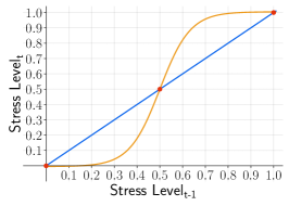
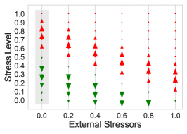
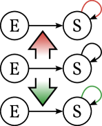
Figure 2: Mechanistic Decomposition as Meta-Causal States. (left) Effect of the stress level on itself (orange) plotted against the identity (blue). Once a threshold of $0.5$ is reached, the function switches behavior from self-suppressing self-reinforcing. (center) Contribution of the stress level mechanism for varying external stressors. Red arrows indicate a self-reinforcing effect, while green arrows indicate suppression. The gray area indicates the system without external stressors. Although all states are governed by the same set of structural equations, our meta-causal analysis identifies mechanistic differences and assigns different behavioral states to the different starting conditions. (right) The standard SCM gets decomposed into different meta-causal states. While the graph adjacency remains the same, the identification function detect the different modes of the causal mechanism. (Best viewed in color.)

Stress is a major cause of fatigue and can lead to other long-term health problems (Maisel et al., 2021; Franklin et al., 2012; Dimsdale, 2008; Bremner, 2006). While short-term exposure may be helpful in enhancing individual performance, long-term stress is detrimental and resilience may decline over time (Wang & Saudino, 2011; Maisel et al., 2021). While actual and perceived stress levels (Cohen et al., 1983; Bremner, 2006; Schlotz et al., 2011; Giannakakis et al., 2019) may vary between individuals (Calkins, 1994; Haggerty, 1996), the overall effect remains the same. We want to model such a system as an example. For simplicity, we present an idealized system that is radically reduced to the only factors of external stress, modeling everyday environmental factors, and the self-influencing level of internal/perceived stress.

We use an identification function to distinguish between two different modes of operation of a causal mechanism. In particular, we are interested whether the inherent dynamics of the internal stress level are self-reinforcing or self-suppressing. For easier analysis of the system we decompose the dynamics of the internal stress variable into a ‘decayed stress’ $d$ and ‘resulting stress’ $s$ computation. The first term are the previous stress levels decayed over time with external factors added. The resulting stress is then the output of a Sigmoidal function (Fig. 2, left) that either reinforces or suppresses the value (Fig. 2,center). The structural equations are defined as follows and we assume that all values lie in the interval of $[0,1]$:

$$f_{d} :=0.95~{}\text{clip}_{[0,1]}(s^{\prime}+0.5\times\text{externalStress})$$

$$f_{s} :=1.01(\frac{1}{1+\text{exp}({-15x+7.5})}-0.5)+0.5$$

where $s$ and $d$ are the resulting and decayed stress levels, and $s^{\prime}$ is the previous stress level of $s$.

We now define the identification function to be $\operatorname{\mathcal{I}}:=\text{sign}(\ddot{f}_{s})$, where $\ddot{f}_{s}$ is the second order derivative of the Sigmoidal $f_{s}$, with either positive or negative effect on the stress level. The described system has two stable modes of dynamics. Note how the second-order inflection point at 0.5 of the Sigmoid acts as a transition point on the behavior of the mechanism. Stress values below 0.5 get suppressed, while values above 0.5 are amplified. Transitions between the two stable states can only be initiated via external stressors. Effectively this results in three possible meta-causal states which are governed via the following transition function:

$$\sigma:(t,s)\mapsto\begin{bmatrix}1&a\\ 0&0\end{bmatrix}\text{~{}with~{}}a:=\text{sign}(\ddot{f}_{s})=\text{sign}(s-0.5)\in\{-1,0,1\}$$

While being rather simple in setup, this example serves as a good demonstration on how dynamical systems induce meta-causal states that exhibit qualitative different behavior although being governed by the same set of underlying structural equations.

Role of Latent Conditioning. A key takeaway in this example is that the current meta-causal state persists due to the current stress levels and system dynamics and not due to a chance in the structural equations. As a consequence, the system can not solely be expressed via some external conditioning factors. In contrast to other examples where system dynamics where purely due to the meta-causal state, here the variable values themselves play a vital role in the overall system dynamics. As a result, the stressed state of a person would persist even when the initiating external stressors disappear. Intervening on the meta-causal state of the system is now ill-defined, as both positive and negative reinforcing effects are governed by the same equation. Thus, creating a disparity between the intervened meta-causal state and the systems’ identified functional behavior.

5 Related Work

Causal Transportability and Reinforcement Learning. Meta-causal models cover cases that reduce to conditionally dependent causal graphs due to changing environments (Peters et al., 2016; Heinze-Deml et al., 2018), but also extend beyond that for dynamical systems. In this sense, the work of Talon et al. (2024) takes a meta-causal view by transporting edges of different causal effects between environments. In general, the transportability of causal relations (Zhang & Bareinboim, 2017; Lee & Bareinboim, 2018; Correa et al., 2022) can be thought of as learning identification functions that have identified the general conditions of the underlying processes to transfer certain types of causal effects between environments Sonar et al. (2021); Yu et al. (2024); Brouillard et al. (2022). This has been studied to some extent under the name of meta-reinforcement learning, which attempts to predict causal relations from the observations of environments Sauter et al. (2023); Dasgupta et al. (2019). Generally, transferability has been considered in reinforcement learning, where the efficient use of data is omnipresent and causality provides guarantees regarding the transferability of the observed mechanisms under changing environments (Sæmundsson et al., 2018; Dasgupta et al., 2019; Zeng et al., 2023).

Large Language Models (LLMs). Meta-causal representations are an important consideration for LLMs and other foundation models, since these models are typically limited to learning world dynamics from purely observational textual descriptions. In order to reason in a truly causal manner, LLMs need to learn meta-causal models (sometimes referred to as ‘world models’) that allow them to simulate the implied consequences of interventions (Lampinen et al., 2024; Li et al., 2021; 2022). To the best of our knowledge, Zečević et al. (2023) made the first attempt to define explicit meta-causal models that integrate with the Pearlian causal framework. However, their proposed models are defined purely as adjacency matrix memorization, such that causal reasoning in LLMs is equivalent to knowledge recall: $(X\rightarrow Y)\Longleftrightarrow(e_{XY}\in\text{Mem})$. Thus, LLMs would not learn the underlying mediation process and would fail to predict the effects of novel interventions on the causal graph.

Actual Causality, Attribution and Cognition. Our MCM framework can also be used to infer and attribute responsibility (as shown in Sec. 4.1) and therefore touches on the topics of fairness, actual causation (AC) and work on counterfactual reasoning in cognitive science. (Von Kügelgen et al., 2022; Karimi et al., 2021; Halpern, 2000; 2016; Chockler & Halpern, 2004; Gerstenberg et al., 2014; Gerstenberg, 2024). The similarities extend to how MCM encourage reasoning about the dependence between actual environmental contingencies and qualitative types of causal mechanisms. In this sense, MCM allow for the direct characterization of actual causes of system dynamics types. A rigorous formalization is left open for future work. While AC in combination with classical SCM only describes relationships between causal variable configurations and observable events, there are cases where we can take an MCM and derive an SCM that encodes the meta-causal types with instrumental variables, thus allowing a similar meta-causal analysis within the AC framework.

6 Conclusion

We formally introduced meta-causal models that are able to capture the dynamics of switching causal types of causal graphs and, in many cases, can better express the qualitative behavior of a causal system under consideration. Within MCM typing mechanisms generalize the notion of specific structural equations and abstract away unnecessary details. We presented a first, motivating example of how a classical causal analysis and a meta-causal perspective can attribute different root causes to the same situation. We extended these claims by considering that MCM are still able to capture and attribute changes in the mechanistic behavior of the system, even though no actual change is apparent. As an application, we presented a first approach to recover metacausal states in the bivariate case. Although our experimental results represent only a first preliminary approach, we find that meta-causal models are a powerful tool for modeling, reasoning, and inferring system dynamics. Finally, we have shown how MCM are able to express more information about a dynamical system than a simple conditioning variable in a standard SCM can do.

Limitations and Future Work. While we have formally introduced meta-causal models, there remain several practical open directions to pursue. First, we have been able to provide examples that illustrate the differences between standard causal, and meta-causal attribution. In particular, the joint application of standard and meta-causal explainability will allow for the joint consideration of actual and mechanistic in future attribution methods. Second, our approach to recover meta-causal states from unlabeled data is open to extension. Discovery on the full causal graphs is a desirable goal that, however, needs further work to reliably control for the changing sets of parents under changing MCS. Finally, we have made a first attempt to present examples for and against the controlling or observational role of meta-causal models. While the observational perspective is mainly of interest for analytical applications, the application of meta-causal models to agent systems and reinforcement learning opens up a new field of application.

Acknowledgments

The TU Darmstadt authors acknowledge the support of the German Science Foundation (DFG) project “Causality, Argumentation, and Machine Learning” (CAML2, KE 1686/3-2) of the SPP 1999 “Robust Argumentation Machines” (RATIO). This work is supported by the Hessian Ministry of Higher Education, Research, Science and the Arts (HMWK; projects “The Third Wave of AI”). It was funded by the European Union. Views and opinions expressed are, however, those of the author(s) only and do not necessarily reflect those of the European Union or the European Health and Digital Executive Agency (HaDEA). Neither the European Union nor the granting authority can be held responsible for them. Grant Agreement no. 101120763 - TANGO. This work was supported from the National High-Performance Computing project for Computational Engineering Sciences (NHR4CES).

The Eindhoven University of Technology authors received support from their Department of Mathematics and Computer Science and the Eindhoven Artificial Intelligence Systems Institute.

Appendix for “Systems with Switching Causal Relations: A Meta-Causal Perspective”

The appendix is structured as follows:

In Sec. A we derive the formula for the theoretical upper bound of the $95\%$ confidence interval. Sec B discusses the sample statistics and convergence results of the applied LO-RANSAC algorithm. Finally, Sec. C discusses the exact parameters of the bivariate meta-causal mechanism data sampling.

Appendix A Probabilities for Sample Computation and Upper Bounds

Consider a dataset $\mathcal{D}\in\mathbf{R}^{m\times 2}$ of $m$ samples over two variables where we want to separate $n$ different functions. We assume that the data distribution contains a uniform number of samples from each function, where each class could be under- or overrepresented by an offset of $\operatorname{d}$. Specifically, we assume that each function is represented by $(1\pm\operatorname{d})\frac{1}{n}|\mathcal{D}|$ samples, i.e., the probability of encountering a particular class $X$ is $\frac{1-\operatorname{d}}{n}\leq P(X)\leq\frac{1+\operatorname{d}}{n}$ and $\mathbb{E}[P(X)]=\frac{1}{n}$. To identify all functions between these two variables, we assume linearity and apply EM with RANSAC on random pairs of samples (see Section 4.2). By selecting $n$ pairs, there is a chance that one pair is chosen from each function (we will refer to such a set of pairs as a “correct” set of samples). In this section, we derive the probability of a correct pair being chosen at random, so that we can estimate how many times pairs need to be sampled to reliably encounter a correct set of samples.

We denote $S$ as the event of “correctly” sampling all $n$ pairs from all $n$ different functions. If all classes have the same number of samples, the chance of randomly selecting a pair from a new class is $\frac{n}{n}\cdot\frac{1}{n}$ for the first pair of samples, $\frac{n-1}{n}\cdot\frac{1}{n}$ for the second, $\dots$, and $\frac{1}{n}\cdot\frac{1}{n}$ for the last; in short:

$$\mathbb{E}[P_{n}(S)]=\frac{n!}{n^{n}}\cdot\left(\frac{1}{n}\right)^{n}=\frac{n!}{n^{2n}}.$$ (1)

If the data distribution is not perfectly uniform, i.e., $\operatorname{d}\neq 0$, we can also calculate a lower bound for the same probability. Consider two probabilities per sample: the probability of selecting a new class $P_{n}(S^{\text{new}})$ and the probability of selecting a second sample of the same class $P_{n}(S^{\text{same}})$ afterwards. Across all samples, these correspond to $\frac{n!}{n^{n}}$ and $(\frac{1}{n})^{n}$ in $\mathbb{E}[P_{n}(S)]$, respectively.

Let us first consider the probability of selecting a new class. When the first sample is taken, only one new class can be selected (probability of 1). If this sample was taken from the largest class first, the probability that subsequent samples will be taken from new classes decreases, since the space of “unsampled” classes is smaller. For this lower bound, we therefore assume that maximally large classes are sampled from as much and as early as possible. According to our assumptions, the largest classes each take up a fraction of $\frac{1+\operatorname{d}}{n}$ of the data. Therefore, the probability of selecting a new class for successive samples has the following probabilities $\frac{n}{n},\frac{n-(1+\operatorname{d})}{n},\frac{n-(1+\operatorname{d})2}{n},\dots$. First, consider the case where $n$ is even. Here, after all the $\frac{n}{2}$ largest classes have been selected, only the small classes remain. For the last, second to last, $\dots$ classes, this probability is represented by $\frac{(1-\operatorname{d})}{n},\frac{2(1-\operatorname{d})}{n},\dots$. Overall, we get the probability

$$P_{n}(S^{\text{new}}_{\text{even}})\geq\left(\prod_{i=\frac{n}{2}}^{n}\frac{n-(1+\operatorname{d})(n-i)}{n}\right)\left(\prod_{i=1}^{\frac{n}{2}-1}\frac{i(1-\operatorname{d})}{n}\right).$$

If $n$ is uneven, an average size class between the largest and smallest classes must be included:

$$P_{n}(S^{\text{new}}_{\text{odd}})\geq\left(\prod_{i=\frac{n}{2}+0.5}^{n}\frac{n-(1+\operatorname{d})(n-i)}{n}\right)\left(\frac{n-(1+\operatorname{d})(\frac{n}{2}-0.5)-1}{n}\right)\left(\prod_{i=1}^{\frac{n}{2}-1.5}\frac{i(1-\operatorname{d})}{n}\right).$$

The probability of selecting a second sample of the same class is easier to calculate. Instead of constant probabilities as in the expectation with $\frac{1}{n}$, we now have two different probabilities in the even case and three in the odd case. In the even case, we have $\frac{n}{2}$ large batches and the same number of small batches, so the probability of choosing the right batch each time is

$$P_{n}(S^{\text{same}}_{\text{even}})\geq\left(\frac{1+\operatorname{d}}{n}\right)^{\frac{n}{2}}\left(\frac{1-\operatorname{d}}{n}\right)^{\frac{n}{2}}.$$

In the uneven case, we also have to also consider the batch that has an average size

$$P_{n}(S^{\text{same}}_{\text{odd}})\geq\left(\frac{1+\operatorname{d}}{n}\right)^{\frac{n}{2}}\frac{1}{n}\left(\frac{1-\operatorname{d}}{n}\right)^{\frac{n}{2}}.$$

Note that for both $P_{n}(S_{\text{new}})$ and $P_{n}(S_{\text{same}})$, the distribution of the data into the largest and smallest possible batches (according to our assumptions) results in the smallest possible probabilities; hence, the computed probability is a lower bound. If the batches were more evenly sized, the probability would be larger. We can also see that a deviation of up to 1 results in a probability of 0, since it is impossible to sample from a class that is not represented in the data.

In total, the probability of selecting of a correct sample set is the product of the two probabilities above, i.e,

$$P_{n}(S)=\begin{cases}P_{n}(S^{\text{new}}_{\text{even}})P_{n}(S^{\text{same}}_{\text{even}})&\text{if }n\text{ is even}\\ P_{n}(S^{\text{new}}_{\text{odd}})P_{n}(S^{\text{same}}_{\text{odd}})&\text{if }n\text{ is odd.}\end{cases}$$ (2)

$P_{n}(S)$ is the (lower bound on the) probability of selecting a correct set of samples. We can calculate the number of trials $k$ needed to find such a set of samples with at least 95% probability. The opposite probability, of never finding it with less than 5% probability, is easier to calculate:

$$(1-P(S))^{k} \leq 1-0.95=0.05$$

$$k\text{ ln}(1-P(S)) \leq\text{ln}(0.05)$$

$$k \leq\frac{\text{ln}(0.05)}{\text{ln}(1-P(S))}$$

This allows us to determine how many attempts might be necessary. Note that while this would leave a 5% chance of not picking the right samples, there are various practical reasons why the actual probability of finding a working set of samples will be higher, e.g., if the number of samples from each class is not as uneven as assumed, or if some samples are distributed in such a way that even picking a sample from the “wrong” class might still lead to the identification of the correct mechanisms.

For example, if $n=2$ and $\operatorname{d}=0.2$, we have an expected probability of $\mathbb{E}[P(S)]=\frac{2!}{2^{2\cdot 2}}=0.125$ and a lower bound of $P_{2}(S)=P(S^{\text{new}}_{\text{even}})P(S^{\text{same}}_{\text{even}})\geq\frac{0.8}{2}\cdot\frac{2}{2}\cdot\frac{1.2}{2}\cdot\frac{0.8}{2}=0.096$. Larger deviations decrease the probability while a deviation of $\operatorname{d}=0$ results in the same probability as with $\mathbb{E}[P(S)]$. For the lower bound, this results in $k=30$ samples for a confidence of 95% using the above calculation steps. All resulting sample counts can be found in Table 2.

K=1

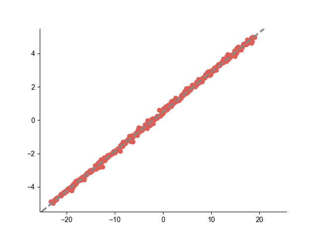
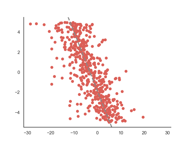
K=2

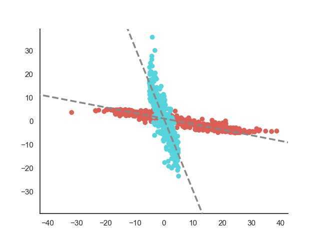
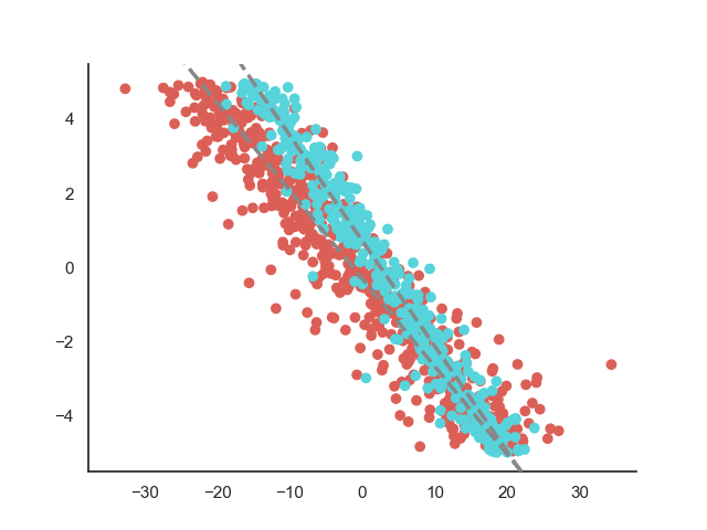
K=3

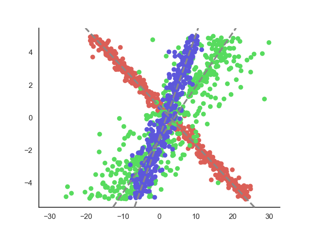
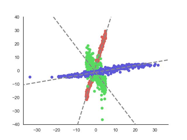
K=4

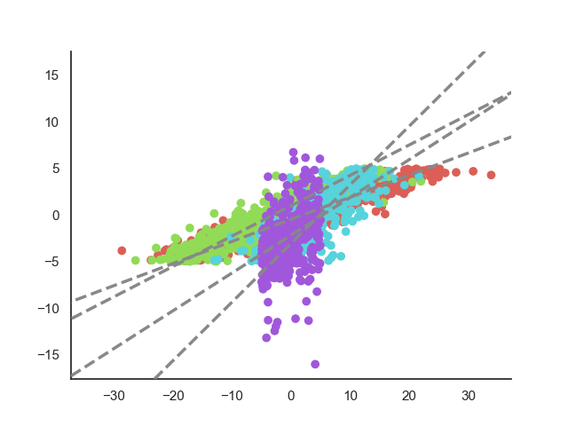
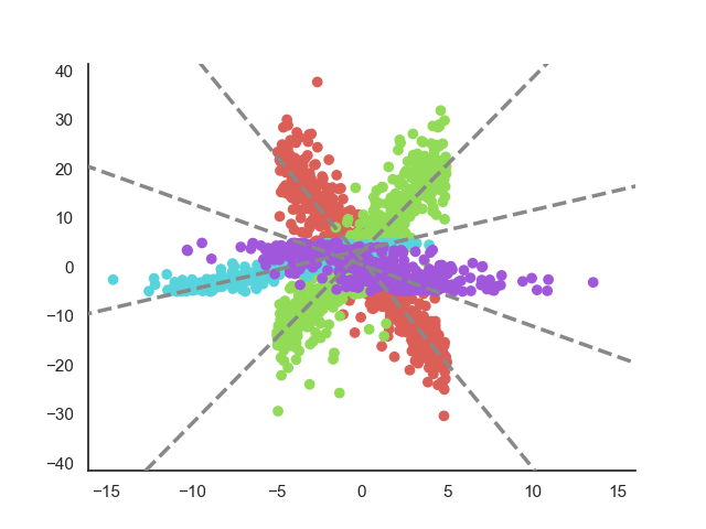
Figure 3: Sampled Mechanisms. The figure shows a selection of different randomly sampled mechanism distributions, ranging from one to up to four simultaneously present mechanisms. The gray dotted lines represent the generating ground truth mechanisms. (Best Viewed In Color)

Appendix B EM Convergence Results

The required number of resamples for a $95\%$ success rate of the RANSAC algorithm is calculated by $\text{log}(0.05)/\text{log}(1-C^{1})$, where $S1$ are the convergence rates for the individual samples computed in Sec. A.

Empirical convergence probabilities and resulting resampling counts for the LO-RANSAC algorithm are shown in Tables 2 and 3. Table 4 lists the goodness of fit for all converged samples. In general, we find that in cases where the approach is able to converge, it undercuts the required parameter convergence boundary of $0.2$ by factors of $4.8$ and $3.5$ for the slope and intercept, respectively.

Class Deviation	1 Mechanism	2 Mechanisms	3 Mechanisms	4 Mechanisms
0.0	${4219}~{}(84.38\%)$	${1740}~{}(34.80\%)$	${592}~{}(11.84\%)$	${86}~{}(1.72\%)$
0.1	"	${1702}~{}(34.04\%)$	${577}~{}(11.54\%)$	${84}~{}(1.68\%)$
0.2	"	${1567}~{}(31.34\%)$	${555}~{}(11.10\%)$	${84}~{}(1.68\%)$

Table 3: Empirical estimated convergence percentage of the EM algorithm for different class imbalances and number of mechanisms. The table shows the number of samples converged and the convergence rates (in parentheses) for a single random initialization and for estimating the parameterization of the underlying system for a given number of mechanisms. All results are reported per 5000 samples.

Class Deviation	1 Mechanism	2 Mechanisms	3 Mechanisms	4 Mechanisms
0.0	$0.0349|0.0590$	$0.0370|0.0543$	$0.0380|0.0592$	$0.0389|0.0516$
0.1	"	$0.0381|0.0555$	$0.0381|0.0566$	$0.0346|0.0528$
0.2	"	$0.0414|0.0548$	$0.0412|0.0567$	$0.0402|0.0570$

Table 4: Mean average error for the slope and intercept of the correctly predicted mechanism for different class imbalances and number of mechanisms. Mechanisms are accepted if their parameters do not differ by more than $0.2$ from the ground truth parameterization. The results show that converged samples are typically estimated with an error well below the threshold.

Appendix C Mechanism Sampling

For our experiments in Sec. 4.2 we uniformly sample the number of mechanisms to be in $K\in\{1..4\}$. The slopes of the linear equations are uniformly sampled between $\alpha\in\pm[0.2..5]$ and the intercepts are in the range $\beta\in[-5,5]$. We add Laplacian noise $\mathcal{L}(x|\mu,b)=\frac{1}{2b}*\exp(-\frac{|x-\mu|}{b})$ with $\mu=0$ and $b\in[0.1,4.0]$. $X$ values are uniformly sampled in the range $[-5,5]$ and $y_{i}=\alpha x_{i}+\beta+\mathcal{L}(x|0,b)$. The average number of samples per class is set to 500. Throughout the experiments, we vary the class probabilities by a class deviation factor $D\in\{0.0,0.1,0.2\}$. Specifically, we maximize the class deviation by assigning $K/2$ classes the maximum probability $1/K*(1+D)$ and $K/2$ classes the minimum probability $1/K*(1-D)$. If $K$ is odd, a class is assigned the average probability $1/K$. We show a selection of the resulting sample distributions in Fig. 3.

Algorithm 1 Recovering Mechanisms for the Bivariate Case

1:procedure RecoverMechanisms($\textbf{x},\textbf{y}$, maxClassDev $K_{\text{max}},\text{EMSteps}$)

2:     for all $k\in[1..K_{\text{max}}]$ do

3:         $\text{bestModelLogL}\leftarrow-\infty$

4:         $\text{N}\leftarrow\text{requiredSamples}(k,\text{maxClassDev},0.95)$ $\triangleright$ Compute $\#$ of samples (c.f. Sec. A)

5:         for all $n\in[1..{\text{N}}]$ do $\triangleright$ RANSAC iteration.

6:              $\textbf{px},\textbf{py}\leftarrow\texttt{sample}(x_{i},y_{i},2*k)$ $\triangleright$ Initialize parameters with $2\times k$ points.

7:              for all $k^{\prime}\in[0..k)$ do

8:                  $\alpha_{k}\leftarrow(py_{2k+1}-py_{2k})/(px_{2k+1}-px_{2k})$

9:                  $\beta_{k}\leftarrow py_{2k}-\alpha_{k}*x_{2k}$

10:                  $b_{k}\leftarrow 1.0$ $\triangleright$ Assume initial avg. deviation of the Laplacion to be 1.

11:                  $d_{k}\leftarrow\text{`XY'}$ $\triangleright$ Assume $X$ $\rightarrow$ $Y$ direction first.

12:                  $\textbf{c}_{k}\leftarrow P_{\texttt{Laplacian}}(\textbf{x},\textbf{y};\alpha,\beta,b,d)$ $\triangleright$ Initial class probabilities for all samples.

13:              end for

14:              for all $l\in[1..\text{EMSteps}]$ do $\triangleright$ EM Iteration.

15:                  $\bm{\alpha},\bm{\beta},\textbf{b},\textbf{d}\leftarrow\texttt{regressLines}(\textbf{x},\textbf{y};\textbf{c})$ $\triangleright$ (Weighted) median regression.

16:                  $\textbf{c}\leftarrow P_{\texttt{Laplacian}}(\textbf{x},\textbf{y};\bm{\alpha},\bm{\beta},\textbf{b},\textbf{d})$

17:              end for

18:              $\text{modelLogL}\leftarrow\sum_{i}\text{LogP}_{\texttt{Laplacian}}(\textbf{x},\textbf{y};\bm{\alpha},\bm{\beta},\textbf{b},\textbf{d})_{i}$ $\triangleright$ Obtain the joint log probs.

19:              if $\text{modelLogL}>\text{bestModelLogL}$ then

20:                  $\text{bestModelLogL}\leftarrow\text{modelLogL}$

21:                  $\text{bestParameters}\leftarrow(\bm{\alpha},\bm{\beta},\textbf{b},\textbf{d})$

22:              end if

23:         end for

24:         $\text{allLaplacian}\leftarrow\texttt{true}$ $\triangleright$ Check if residuals are Laplacian distributed.

25:         for all $l\in[1..k]$ do

26:              $(\bm{\alpha},\bm{\beta},\textbf{b},\textbf{d})\leftarrow\text{bestParameters}$

27:              $\textbf{x}^{l},\textbf{y}^{l},\textbf{c}^{l}\leftarrow\texttt{selectClass}(\textbf{x},\textbf{y},\textbf{c},l)$ $\triangleright$ Select points where $\text{argmax}_{\textbf{c}}=l$.

28:              $\textbf{x}^{l},\textbf{y}^{l}\leftarrow\texttt{filter}(\textbf{x}^{l},\textbf{y}^{l},\textbf{c}^{l},0.4)$ $\triangleright$ Keep points s.t. $\text{max}^{\#2}\textbf{c}^{l}<0.4(1-\text{max}^{\#1}(\textbf{c}^{l})$.

29:              $r=\texttt{LinEq}(\textbf{x}^{l},\textbf{y}^{l};\alpha_{l},\beta_{l},d_{l})-\textbf{y}^{l}$

30:              if $\textbf{not~{}}\texttt{AndersonDarling}(r,0.95)$ then

31:                  $\text{allLaplacian}\leftarrow\texttt{false}$

32:                  break

33:              end if

34:         end for

35:         if allLaplacian then

36:              return k

37:         end if

38:     end for

39:     return 0

40:end procedure

References

- Anand et al. (2022) Tara V Anand, Adèle H Ribeiro, Jin Tian, and Elias Bareinboim. Effect identification in cluster causal diagrams. arXiv preprint arXiv:2202.12263, 2022.
- Anderson & Darling (1952) Theodore W Anderson and Donald A Darling. Asymptotic theory of certain” goodness of fit” criteria based on stochastic processes. The annals of mathematical statistics, pp. 193–212, 1952.
- Arnellos et al. (2006) Argyris Arnellos, Thomas Spyrou, and John Darzentas. Dynamic interactions in artificial environments: causal and non-causal aspects for the emergence of meaning. Systemics, Cybernetics and Informatics, 3:82–89, 2006.
- Beckers & Halpern (2019) Sander Beckers and Joseph Y Halpern. Abstracting causal models. In Proceedings of the aaai conference on artificial intelligence, volume 33, pp. 2678–2685, 2019.
- Bellman (1957) Richard Bellman. A markovian decision process. Journal of mathematics and mechanics, pp. 679–684, 1957.
- Bremner (2006) J Douglas Bremner. Traumatic stress: effects on the brain. Dialogues in clinical neuroscience, 8(4):445–461, 2006.
- Brouillard et al. (2022) Philippe Brouillard, Perouz Taslakian, Alexandre Lacoste, Sébastien Lachapelle, and Alexandre Drouin. Typing assumptions improve identification in causal discovery. In Conference on Causal Learning and Reasoning, pp. 162–177. PMLR, 2022.
- Calkins (1994) SD Calkins. Origins and outcomes of individual differences in emotion regulation. The Development of Emotion Regulation: Biological and Behavioral Considerations, Monographs of the Society for Research in Child Development, 59(2-3), 1994.
- Chen (2002) Colin Chen. Tests for the goodness-of-fit of the laplace distribution. Communications in Statistics-Simulation and Computation, 31(1):159–174, 2002.
- Chockler & Halpern (2004) Hana Chockler and Joseph Y Halpern. Responsibility and blame: A structural-model approach. Journal of Artificial Intelligence Research, 22:93–115, 2004.
- Chum et al. (2003) Ondřej Chum, Jiří Matas, and Josef Kittler. Locally optimized ransac. In Pattern Recognition: 25th DAGM Symposium, Magdeburg, Germany, September 10-12, 2003. Proceedings 25, pp. 236–243. Springer, 2003.
- Cohen et al. (1983) Sheldon Cohen, Tom Kamarck, and Robin Mermelstein. A global measure of perceived stress. Journal of health and social behavior, pp. 385–396, 1983.
- Cohen (2022) Taco Cohen. Towards a grounded theory of causation for embodied ai. arXiv preprint arXiv:2206.13973, 2022.
- Correa et al. (2022) Juan D Correa, Sanghack Lee, and Elias Bareinboim. Counterfactual transportability: a formal approach. In International Conference on Machine Learning, pp. 4370–4390. PMLR, 2022.
- Dasgupta et al. (2019) Ishita Dasgupta, Jane Wang, Silvia Chiappa, Jovana Mitrovic, Pedro Ortega, David Raposo, Edward Hughes, Peter Battaglia, Matthew Botvinick, and Zeb Kurth-Nelson. Causal reasoning from meta-reinforcement learning. arXiv preprint arXiv:1901.08162, 2019.
- Dempster et al. (1977) Arthur P Dempster, Nan M Laird, and Donald B Rubin. Maximum likelihood from incomplete data via the em algorithm. Journal of the royal statistical society: series B (methodological), 39(1):1–22, 1977.
- Dimsdale (2008) Joel E Dimsdale. Psychological stress and cardiovascular disease. Journal of the American College of Cardiology, 51(13):1237–1246, 2008.
- Fischler & Bolles (1981) Martin A Fischler and Robert C Bolles. Random sample consensus: a paradigm for model fitting with applications to image analysis and automated cartography. Communications of the ACM, 24(6):381–395, 1981.
- Franklin et al. (2012) Tamara B Franklin, Bechara J Saab, and Isabelle M Mansuy. Neural mechanisms of stress resilience and vulnerability. Neuron, 75(5):747–761, 2012.
- Gerstenberg (2022) Tobias Gerstenberg. What would have happened? counterfactuals, hypotheticals and causal judgements. Philosophical Transactions of the Royal Society B, 377(1866):20210339, 2022.
- Gerstenberg (2024) Tobias Gerstenberg. Counterfactual simulation in causal cognition. Trends in Cognitive Sciences, 2024.
- Gerstenberg et al. (2014) Tobias Gerstenberg, Noah Goodman, David Lagnado, and Josh Tenenbaum. From counterfactual simulation to causal judgment. In Proceedings of the annual meeting of the cognitive science society, volume 36, 2014.
- Giannakakis et al. (2019) Giorgos Giannakakis, Dimitris Grigoriadis, Katerina Giannakaki, Olympia Simantiraki, Alexandros Roniotis, and Manolis Tsiknakis. Review on psychological stress detection using biosignals. IEEE transactions on affective computing, 13(1):440–460, 2019.
- Haggerty (1996) Robert J Haggerty. Stress, risk, and resilience in children and adolescents: Processes, mechanisms, and interventions. Cambridge University Press, 1996.
- Halpern (2000) Joseph Y Halpern. Axiomatizing causal reasoning. Journal of Artificial Intelligence Research, 12:317–337, 2000.
- Halpern (2016) Joseph Y Halpern. Actual causality. MiT Press, 2016.
- Heinze-Deml et al. (2018) Christina Heinze-Deml, Jonas Peters, and Nicolai Meinshausen. Invariant causal prediction for nonlinear models. Journal of Causal Inference, 6(2):20170016, 2018.
- Hofmann et al. (2020) Stefan G Hofmann, Joshua E Curtiss, and Steven C Hayes. Beyond linear mediation: Toward a dynamic network approach to study treatment processes. Clinical Psychology Review, 76:101824, 2020.
- Hoyer et al. (2008) Patrik Hoyer, Dominik Janzing, Joris M Mooij, Jonas Peters, and Bernhard Schölkopf. Nonlinear causal discovery with additive noise models. Advances in neural information processing systems, 21, 2008.
- Karimi et al. (2021) Amir-Hossein Karimi, Bernhard Schölkopf, and Isabel Valera. Algorithmic recourse: from counterfactual explanations to interventions. In Proceedings of the 2021 ACM conference on fairness, accountability, and transparency, pp. 353–362, 2021.
- Kekić et al. (2023) Armin Kekić, Bernhard Schölkopf, and Michel Besserve. Targeted reduction of causal models. In ICLR 2024 Workshop on AI4DifferentialEquations In Science, 2023.
- Lampinen et al. (2024) Andrew Lampinen, Stephanie Chan, Ishita Dasgupta, Andrew Nam, and Jane Wang. Passive learning of active causal strategies in agents and language models. Advances in Neural Information Processing Systems, 36, 2024.
- Lee & Bareinboim (2018) Sanghack Lee and Elias Bareinboim. Structural causal bandits: Where to intervene? Advances in neural information processing systems, 31, 2018.
- Li et al. (2021) Belinda Z Li, Maxwell Nye, and Jacob Andreas. Implicit representations of meaning in neural language models. arXiv preprint arXiv:2106.00737, 2021.
- Li et al. (2022) Kenneth Li, Aspen K Hopkins, David Bau, Fernanda Viégas, Hanspeter Pfister, and Martin Wattenberg. Emergent world representations: Exploring a sequence model trained on a synthetic task. arXiv preprint arXiv:2210.13382, 2022.
- Maisel et al. (2021) Peter Maisel, Erika Baum, and Norbert Donner-Banzhoff. Fatigue as the chief complaint: epidemiology, causes, diagnosis, and treatment. Deutsches Ärzteblatt International, 118(33-34):566, 2021.
- Moore et al. (1956) Edward F Moore et al. Gedanken-experiments on sequential machines. Automata studies, 34:129–153, 1956.
- Pearl (2009) Judea Pearl. Causality. Cambridge university press, 2009.
- Peters et al. (2016) Jonas Peters, Peter Bühlmann, and Nicolai Meinshausen. Causal inference by using invariant prediction: identification and confidence intervals. Journal of the Royal Statistical Society Series B: Statistical Methodology, 78(5):947–1012, 2016.
- Rubenstein et al. (2017) Paul K Rubenstein, Sebastian Weichwald, Stephan Bongers, Joris M Mooij, Dominik Janzing, Moritz Grosse-Wentrup, and Bernhard Schölkopf. Causal consistency of structural equation models. arXiv preprint arXiv:1707.00819, 2017.
- Sæmundsson et al. (2018) Steindór Sæmundsson, Katja Hofmann, and Marc Peter Deisenroth. Meta reinforcement learning with latent variable gaussian processes. arXiv preprint arXiv:1803.07551, 2018.
- Sauter et al. (2023) Andreas WM Sauter, Erman Acar, and Vincent Francois-Lavet. A meta-reinforcement learning algorithm for causal discovery. In Conference on Causal Learning and Reasoning, pp. 602–619. PMLR, 2023.
- Schlotz et al. (2011) Wolff Schlotz, Ilona S Yim, Peggy M Zoccola, Lars Jansen, and Peter Schulz. The perceived stress reactivity scale: measurement invariance, stability, and validity in three countries. Psychological assessment, 23(1):80, 2011.
- Schölkopf et al. (2012) Bernhard Schölkopf, Dominik Janzing, Jonas Peters, Eleni Sgouritsa, Kun Zhang, and Joris Mooij. On causal and anticausal learning. arXiv preprint arXiv:1206.6471, 2012.
- Sloman et al. (2009) Steven A Sloman, Philip M Fernbach, and Scott Ewing. Causal models: The representational infrastructure for moral judgment. Psychology of learning and motivation, 50:1–26, 2009.
- Sonar et al. (2021) Anoopkumar Sonar, Vincent Pacelli, and Anirudha Majumdar. Invariant policy optimization: Towards stronger generalization in reinforcement learning. In Learning for Dynamics and Control, pp. 21–33. PMLR, 2021.
- Spirtes et al. (2000) Peter Spirtes, Clark N Glymour, Richard Scheines, and David Heckerman. Causation, prediction, and search. MIT press, 2000.
- Talon et al. (2024) Davide Talon, Phillip Lippe, Stuart James, Alessio Del Bue, and Sara Magliacane. Towards the reusability and compositionality of causal representations. arXiv preprint arXiv:2403.09830, 2024.
- Von Kügelgen et al. (2022) Julius Von Kügelgen, Amir-Hossein Karimi, Umang Bhatt, Isabel Valera, Adrian Weller, and Bernhard Schölkopf. On the fairness of causal algorithmic recourse. In Proceedings of the AAAI conference on artificial intelligence, volume 36, pp. 9584–9594, 2022.
- Wahl et al. (2023) Jonas Wahl, Urmi Ninad, and Jakob Runge. Foundations of causal discovery on groups of variables. arXiv preprint arXiv:2306.07047, 2023.
- Walsh & Sloman (2011) Clare R Walsh and Steven A Sloman. The meaning of cause and prevent: The role of causal mechanism. Mind & Language, 26(1):21–52, 2011.
- Wang & Saudino (2011) Manjie Wang and Kimberly J Saudino. Emotion regulation and stress. Journal of Adult Development, 18:95–103, 2011.
- Willig et al. (2023) Moritz Willig, Matej Zečević, Devendra Singh Dhami, and Kristian Kersting. Do not marginalize mechanisms, rather consolidate! In Proceedings of the 37th Conference on Neural Information Processing Systems (NeurIPS), 2023.
- Wolff (2007) Phillip Wolff. Representing causation. Journal of experimental psychology: General, 136(1):82, 2007.
- Yu et al. (2024) Zhongwei Yu, Jingqing Ruan, and Dengpeng Xing. Learning causal dynamics models in object-oriented environments. arXiv preprint arXiv:2405.12615, 2024.
- Zečević et al. (2023) Matej Zečević, Moritz Willig, Devendra Singh Dhami, and Kristian Kersting. Causal parrots: Large language models may talk causality but are not causal. Transactions on Machine Learning Research, 2023.
- Zeng et al. (2023) Yan Zeng, Ruichu Cai, Fuchun Sun, Libo Huang, and Zhifeng Hao. A survey on causal reinforcement learning. arXiv preprint arXiv:2302.05209, 2023.
- Zhang & Bareinboim (2017) Junzhe Zhang and Elias Bareinboim. Transfer learning in multi-armed bandit: a causal approach. In Proceedings of the 16th Conference on Autonomous Agents and MultiAgent Systems, pp. 1778–1780, 2017.