Synthesis and Perceptual Scaling of High Resolution Natural Images Using Stable Diffusion

Abstract

Natural scenes are of key interest for visual perception. Previous work on natural scenes has frequently focused on collections of discrete images with considerable physical differences from stimulus to stimulus. For many purposes it would, however, be desirable to have sets of natural images that vary smoothly along a continuum (for example in order to measure quantitative properties such as thresholds or precisions). This problem has typically been addressed by morphing a source into a target image. However, this approach yields transitions between images that primarily follow their low-level physical features and that can be semantically unclear or ambiguous. Here, in contrast, we used a different approach (Stable Diffusion XL) to synthesise a custom stimulus set of photorealistic images that are characterized by gradual transitions where each image is a clearly interpretable but unique exemplar from the same category. We developed natural scene stimulus sets from six categories with 18 objects each. For each object we generated 10 graded variants that are ordered along a perceptual continuum. We validated the image set psychophysically in a large sample of participants, ensuring that stimuli for each exemplar have varying levels of perceptual confusability. This image set is of interest for studies on visual perception, attention and short- and long-term memory.

1 Introduction

Naturalistic stimuli are important for understanding object recognition and memory in ecologically valid settings [1, 2, 3, 4], but they present several challenges. They can vary widely in their semantic and perceptual dimensions, which makes them harder to select and to control experimentally in comparison to low-dimensional stimuli [5]. In contrast to traditional stimulus sets, which have relied on the manual selection of a limited set of cropped images [6, 7] — a process that is both time-consuming and susceptible to subjectivity biases - recent attempts have strived to systematically collect and use naturalistic stimuli. These approaches are usually “bottom-up”, involving the collection and categorization of large numbers of images from the internet (“scraping”). These can be found in large-scale image datasets used in the machine learning community for computer vision tasks, such as ImageNet [8] or the Microsoft Common Objects in Context (COCO) dataset [9]. For example, this was the case for the Natural Scenes Dataset (NSD) initiative [10], which provides a rich amount of behavioral and neuroimaging data collected while participants viewed scenes from the COCO dataset. Such stimuli, however, are not always ideally suited for cognitive tasks and often require manual pre-selection. To address this issue, the THINGS initiative [11] has developed a procedure to sample and evaluate a vast variety of “object concepts” from the web, specifically tailored for cognitive scientific tasks. Despite these advancements, these methods remain fundamentally dependent on existing images and their post hoc categorisation.

An alternative approach involves synthesizing stimuli using modern machine learning technology. Generative models such as Variational Autoencoders (VAEs) [12], Generative Adversarial Networks (GANs) [13] and Diffusion Models (DMs) [14] have already provided novel methodological approaches to many areas of neuroscience, including image reconstruction from neuroimaging data [15, 16, 17], analysis of neural population dynamics [18, 19], and clinical imaging [20, 21]. They are also promising for the synthetic generation of naturalistic-appearing stimuli for experimental tasks [5, 22, 23]. Compared to “bottom-up” approaches that rely on scraping pre-existing images from the web, generative models allow for the synthesis of virtually unlimited high-resolution images, removing the dependency on existing sources. This is particularly appealing for object recognition and memory research, as it enables the creation of a variety of objects from a wide range of categories.

One particularly interesting feature of artificially generated images is that they can potentially help tackle the trade-off between ecological validity and parametric experimental control. For example, low-level physical properties (such as orientation or luminance) can easily be gradually varied and they are thus suitable for psychophysical studies that involve assessment of quantitative properties such as detection thresholds or precision [24]. In contrast, sets of discrete natural images do not exhibit the same kind of gradual local ordering that would be necessary for such quantitative assessments. Any measurement that requires gradual variation of an image property is very difficult to realize with sets of pre-existing, discrete naturalistic stimuli.

Controlling perceptual and semantic features of high-dimensional naturalistic stimuli is inherently difficult. Here, we aim to fill in this gap. We propose a method for establishing sets of experimental stimuli that generates multiple variants of a scene containing a natural object that vary perceptually along a gradual scale. One class of machine learning methods, Generative Adversarial Networks (GANs) [13], have recently gained attention in cognitive science [5]. The deep generative representations that GANs learn have been shown to be structured semantically [25]. They allow obtaining fine-grained and relatively selective variations of the images along continuous dimensions, both for perceptual (e.g. the lightness of the scene) and for semantic features (e.g. facial attributes) [26, 27]. For example, Son et al. [22] used a GAN to create “scene wheels” of naturalistic indoor scenes with varying levels of similarity, which they employed in a visual working memory task, typically used for simpler features like color or orientation [28]. This reflects a growing interest towards a more ecologically valid assessment of cognitive function and provides the possibility to extend working memory models to naturalistic stimuli [29].

Despite their utility, GANs face significant limitations. Their training is computationally expensive and susceptible to mode collapse [30, 31], where the generator network over-optimizes for images that the discriminator network finds highly plausible, leading to the repeated production of a limited set of similar images and compromising the variety of generated samples. Additionally, pre-trained GAN models, while available [32], often require fine-tuning to be suitable for specific image generation tasks. Some of these models can generate a variety of images but are restricted to certain categories and their resolution can be rather low. Importantly, morphing between images often results in unnatural artefacts. These limitations suggest that GANs may not always be suitable for generating stimuli for experiments in cognitive science.

Another class of generative neural networks specialised in image synthesis is diffusion models [14, 33, 34], which so far have received less attention in cognitive science. Stable Diffusion [35] in particular is an open-source model that can generate images from text prompts, which is considerably more flexible [36]. This also allows for a strong link between semantic and image levels of representation. In this study, we present a novel set of naturalistic stimuli generated using Stable Diffusion XL [37], a diffusion model that excels in the synthesis of high resolution images (1024x1024 pixels), and we show a method relying on interpolation to generate naturalistic stimuli along a continuous perceptual scale. This method makes it possible to create image sets that are perceptually distinct, yet maintaining consistent semantic meaning. This feature is particularly promising for research in visual memory, attention, and object recognition, as it allows for precise manipulation of perceptual differences without altering significantly the underlying semantic content. We validated the dataset through an online similarity judgement task, involving a sample of 1113 participants. The results confirmed that our stimuli effectively captured perceptual variations, making them a useful resource for studying memory and perception under controlled yet ecologically valid conditions. By providing these datasets publicly (see Data Availability section), we hope to contribute a valuable tool for the research community, bridging the gap between ecological validity and experimental control in visual cognition studies.

2 Overview of Methods

The image generation proceeded in six steps (shown in Figure 1):

(S1) We used Stable Diffusion in combination with text prompts to generate naturalistic images with a clear, central object situated in a coherent scene, rich in detail. Since text-to-image models [38] can generate multiple images from a textual prompt, there are potentially infinite images that can be synthesized. We therefore narrowed down the prompt space by defining 6 different categories from which our objects were taken. These categories were split into natural (animals, plants, landscape elements) and artificial (vehicles, items, buildings). For each category, we identified 18 unique objects that were distinct yet representative of the category (Table 1). For each object, we defined a unique text prompt.

(S2) Based on these text prompts, we used Stable Diffusion XL [37] to generate 60 exemplar images per object and category as a starting point. These were different versions of the same scene.

(S3) For each pair of these 60 exemplar images, we computed a coarse-grained model-based perceptual similarity score using an established metric based on neural network activation patches, the Learned Perceptual Image Patch Similarity (LPIPS) metric [39]. From this, we selected an “anchor image” and a “guide image”. These two images were chosen such that they were representative of the set as well as perceptually similar to one another (see below).

(S4) We then used spherical interpolation to yield 200 images per object on the continuum between the anchor image and the guide image. This interpolation was done at the level of noise latents (see Appendix for details) rather than at the semantic level of the text prompts in order to ensure that interpolated images varied perceptually but not in terms of meaning.

(S5) We used the artificial neural network model once more to compute the fine-grained model-based perceptual similarity between these 200 interpolations. Based on this, we selected a total of ten images that were dissimilar from the anchor image in an approximately linear way.

(S6) We then used an online crowdsourcing task with 1113 participants to validate the ordering of the 10 interpolated images using a psychophysical similarity judgement task. We used these crowd judgements to fine-tune the order to match up with the psychophysical judgements (this was done in order to allow us to correct any inaccuracy in the way the computational model estimated the similarity).

This procedure yielded 108 sets of 10 continuously varying stimuli, each set for a specific object from a specific category.

Category	Objects
animal	beaver, butterfly, cat, dog, elephant, fish, frog, giraffe, horse, koala, leopard, lizard, owl, parrot, penguin, seal, tortoise, tropical_bird
building	adobe_house, bamboo_house, barn, bell_tower, cabin, farm, fortress, futuristic_building, greenhouse, igloo, lighthouse, modern_building, observatory, pagoda, polar_base, skyscraper, tea_house, windmill
item	basket, bottle, candlestick, chair, coffee_mug, hourglass, jar, lamp_standing, lamp_table, lantern, mortar, pot, shovel, sofa, teapot, telescope, vase, wheelbarrow
landscape_element	desert_arch, desert_butte, fjord_pillar, forest_boulder, forest_river, geothermal_spring, grassland_monolith, hill_river, lake_island, moorland_tor, mountain_glacier, mountain_ridge, mountain_rock, polar_iceberg, sea_stack, tropical_karst, volcanic_peak, wetland_tufa
plant	acacia, baobab, birch, bristlecone, cactus, cherry, dragon_tree, eucalyptus, kapok, magnolia, maple, oak, olive, palm, pine, pine_med, sequoia, willow
vehicle	campervan, car_vintage, fishing_boat, hot_air_balloon, jet_plane, lorry, motorcycle, offroad_vehicle, passenger_train, rowing_boat, sailboat, scooter, seaplane, space_rocket, sports_car, steam_locomotive, tourist_helicopter, tractor

Table 1: Overview of the six categories and their corresponding objects: three natural/living (animals, plants, landscape elements) and three artificial/non-living (items, buildings, vehicles), each with 18 diverse objects.

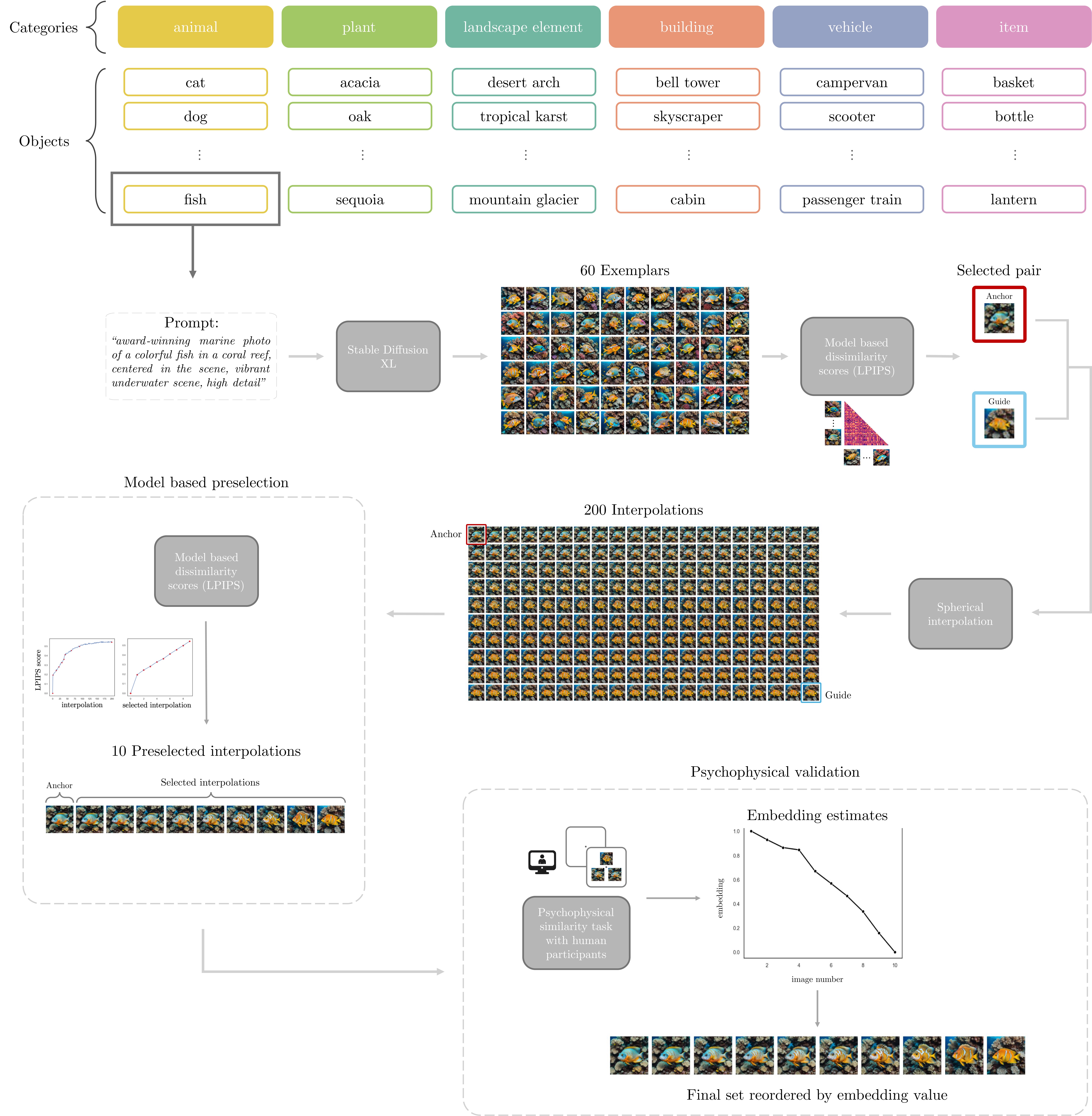
Figure 1: Overview of the pipeline to generate the stimulus set. We defined six global categories (three natural and three artificial), each including eighteen object scenes. To generate varied exemplar images for each object (here “fish”), we used a single prompt, and variability was induced by using sixty starting noise latents (see Methods). From each set of exemplar images, we selected an anchor and a guide image for the interpolation, which was performed between their respective noise latents. Out of 200 interpolated images, we pre-selected 10 (the anchor image and nine interpolations) using a computational model-based metric (LPIPS, [39]) as an initial approximation to quantify their perceptual similarity. We then conducted an online similarity judgment task using triplet comparisons (see Appendix) to confirm and potentially fine-tune the order for each object set. The bottom right plot shows the final order of stimuli and the corresponding embedding values (see Appendix) for an example interpolation sequence of one object (fish). The x-axis shows the ten images, and the y-axis shows the psychophysical embedding score. Relative distances on this embedding score correspond to perceptual differences.

3 Results

In the first steps (S1-S2), our procedure generated 60 exemplar images for 18 objects taken out of six categories. Figure 2 shows examples for each of the 18 objects in the 3 categories of natural stimuli, and Figure 3 shows examples for each of the 18 objects in the three artificial categories. Out of the 60 exemplar images created for each object we selected an anchor and a guide image (see Appendix). Figure  3 shows the anchor images that were used as a starting point for the subsequent interpolation.

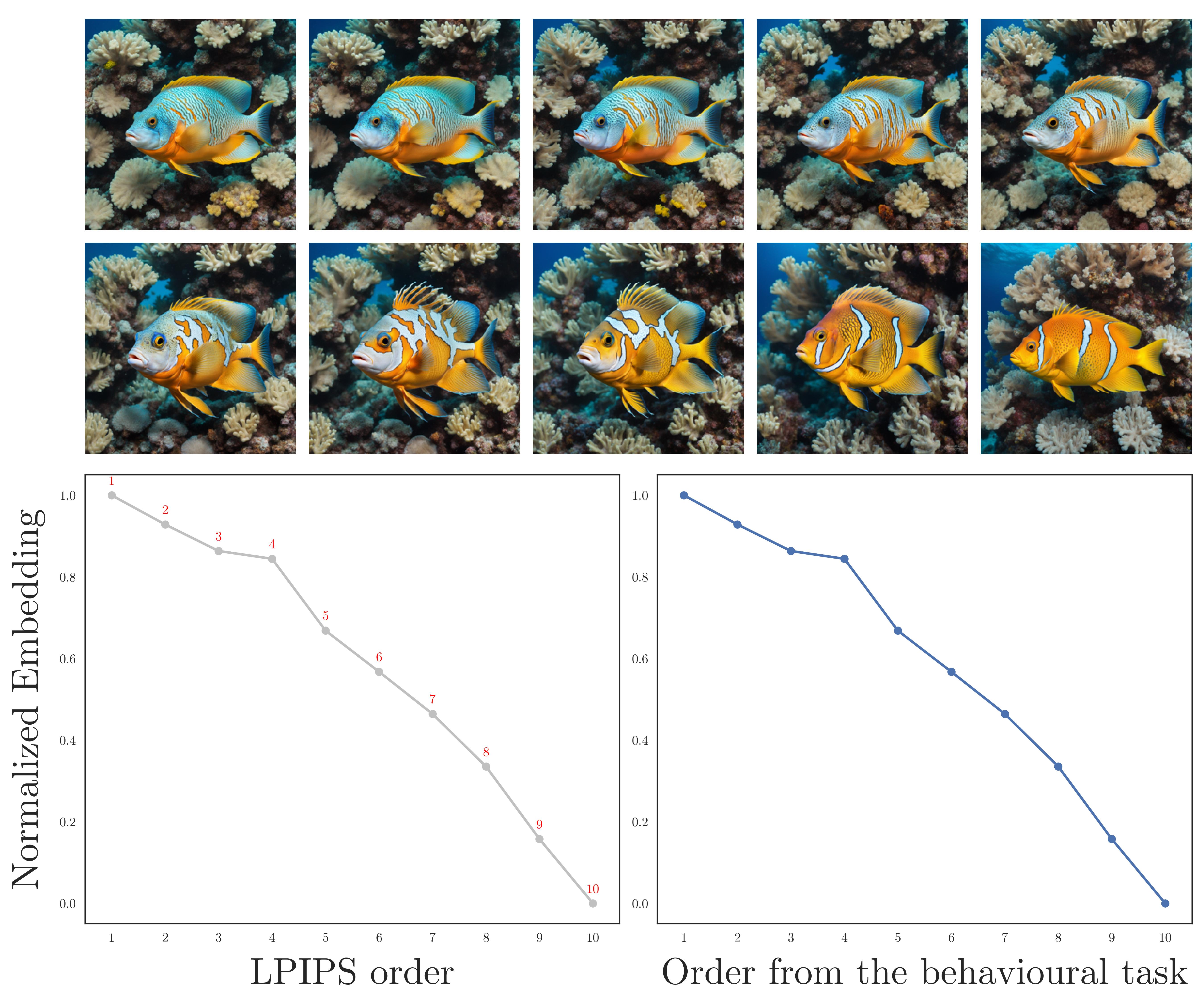
(a)

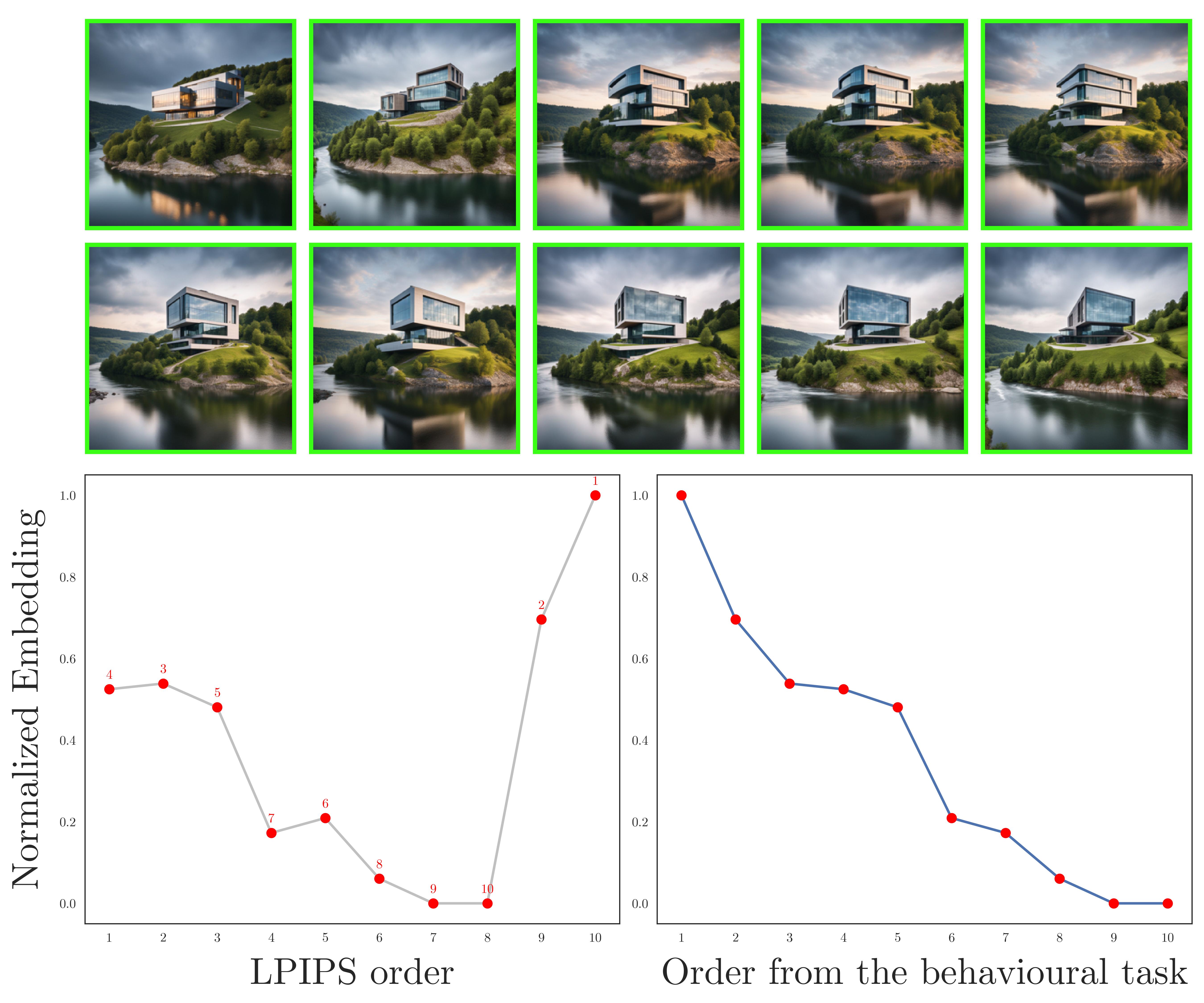
(b)

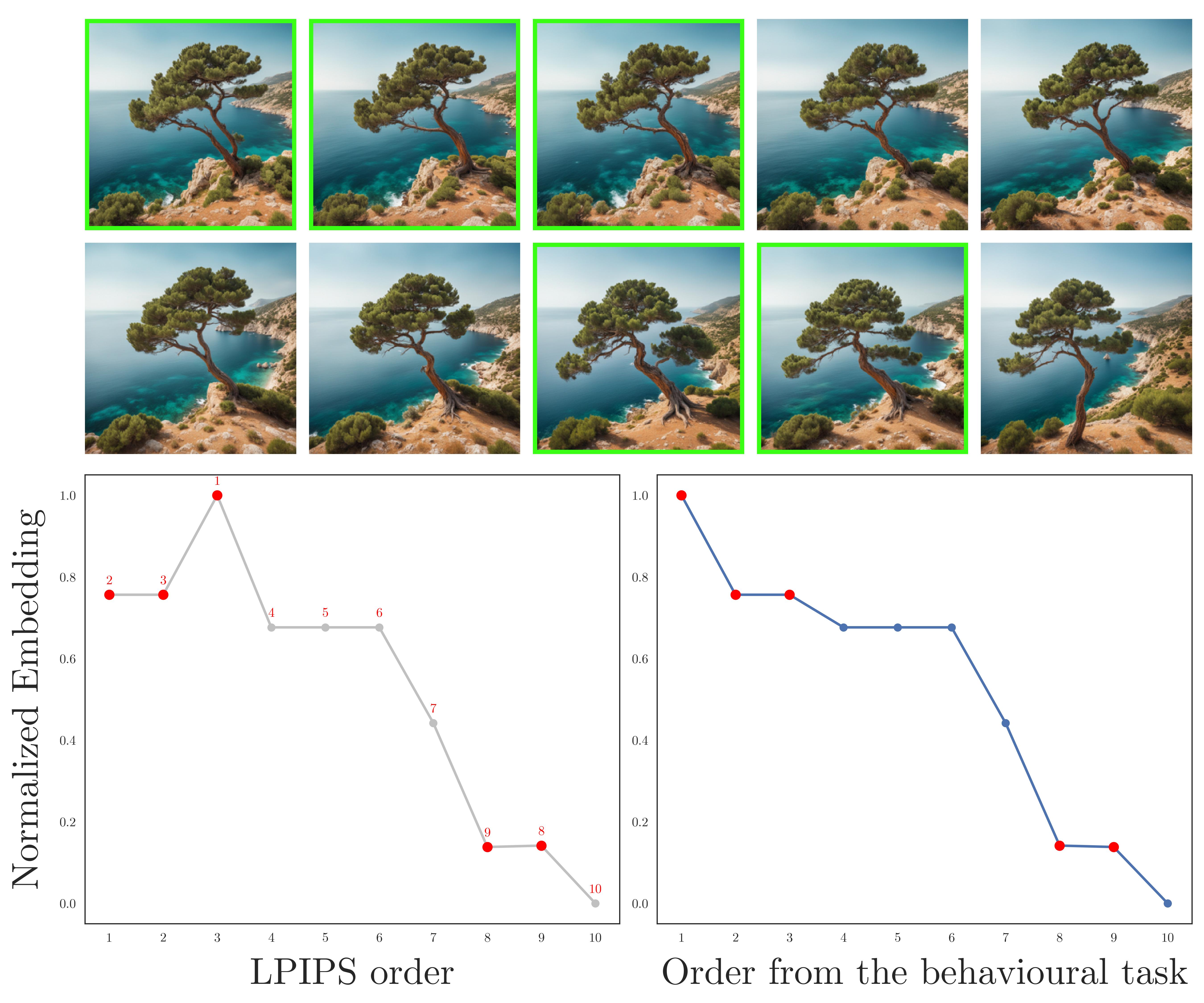
(c)

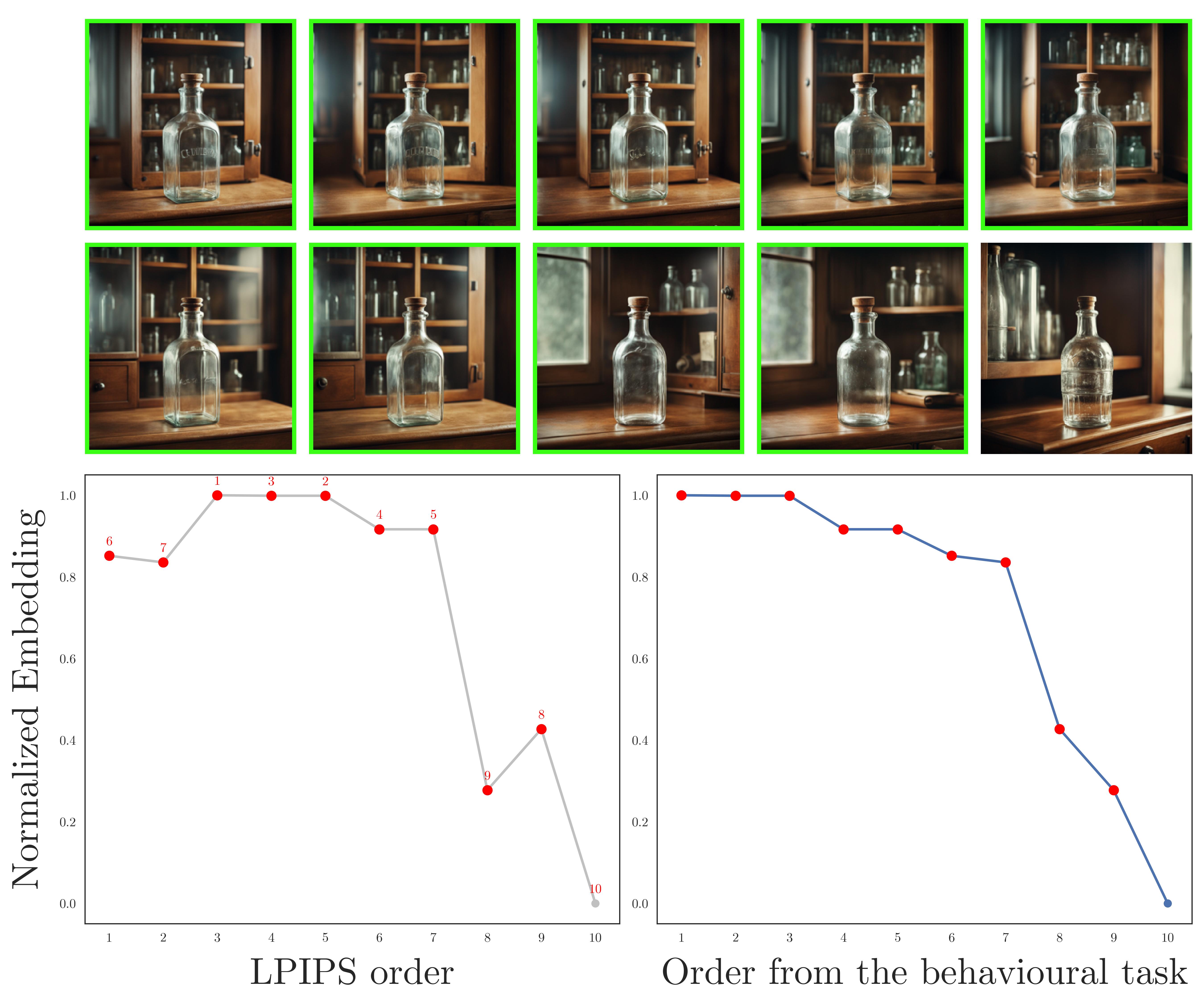
(d)

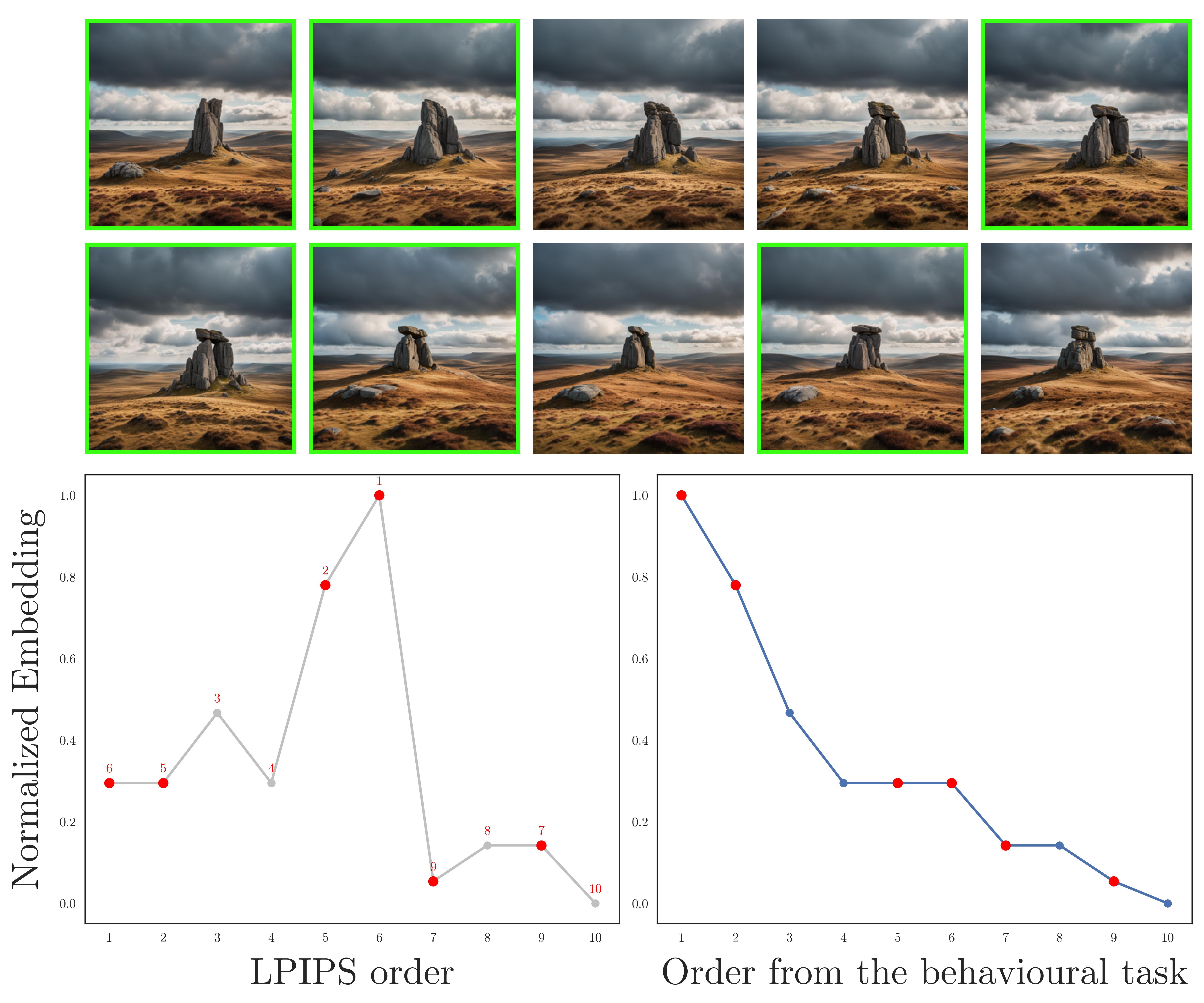
(e)

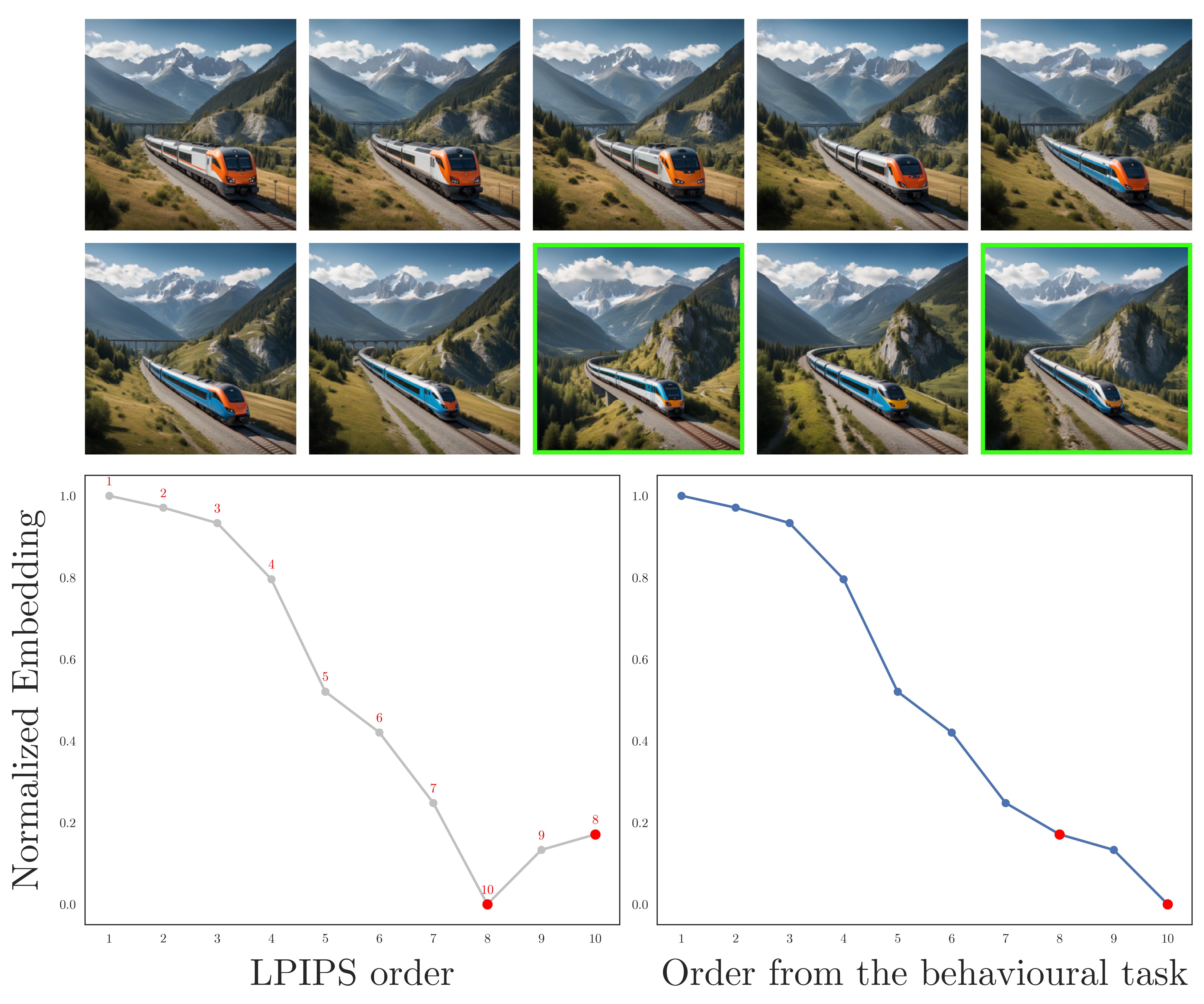
(f)

Figure 22: Example reorderings based on embedding values. Each panel displays images ordered by their embedding values. Images where the order was changed compared to the LPIPS model are highlighted in green. The left plot shows the original order, with red numbers indicating new positions post-reordering. The right plot displays the reordered objects sorted by embedding value. The x-axis represents object positions, while the y-axis shows embedding values. Red dots mark changed positions, highlighting adjustments in object order. Panels: a) fish, b) modern building, c) Pine (Mediterranean), d) bottle, e) moorland tor, f) passenger train.

In the next steps (S3-S6) our procedure generated a perceptually ordered set of 10 images for each object. Specifically, each set comprised 10 slightly different realisations of the same object, each of which being clearly perceivable as belonging to its object category. Within each object set the images formed a perceptual continuum. Figure 4 shows these image sets for two selected object exemplars for each of the 18 categories. The image sets are characterized by gradual transitions the order of which was validated in an online psychophysical task. The boxes in Figure 2 and Figure 3 show the examples for which interpolations are shown in Figure 4. As can be seen, the interpolation at the level of “noise latents” (see Appendix A.3) successfully ensured that all images within the set were different realizations of the same meaning. An example of the ordering based on the psychophysics task can be seen in Figure 1 (bottom right). More orderings based on the LPIPS model and their fine-tuning based on the psychophysics can be found in Figure 22. The psychophysical validation of the similarity structure based on the online experiment yielded that a total of 88% objects required at least one position reordering (cf. Appendix B.3).

We took further steps to ensure that the image sequences were perceptually valid. We implemented a systematic process to exclude images with artifacts, resulting in a 3.3% exclusion rate (Figure 11). Some interpolated images had to be replaced if they exhibited such inconsistencies (see Appendix B.1; Figure 14; Table LABEL:tab:exclusion-rates-exemplars). We also checked whether there were any overall differences in model-based similarity scores across the different categories. We found that only buildings and items deviated in their scores (for full details, see Appendix B.1.2). Furthermore, we assessed physical properties of the anchor images and found they were similar across categories (Figures 17(a) and 17(b) in Appendix B.1.4).

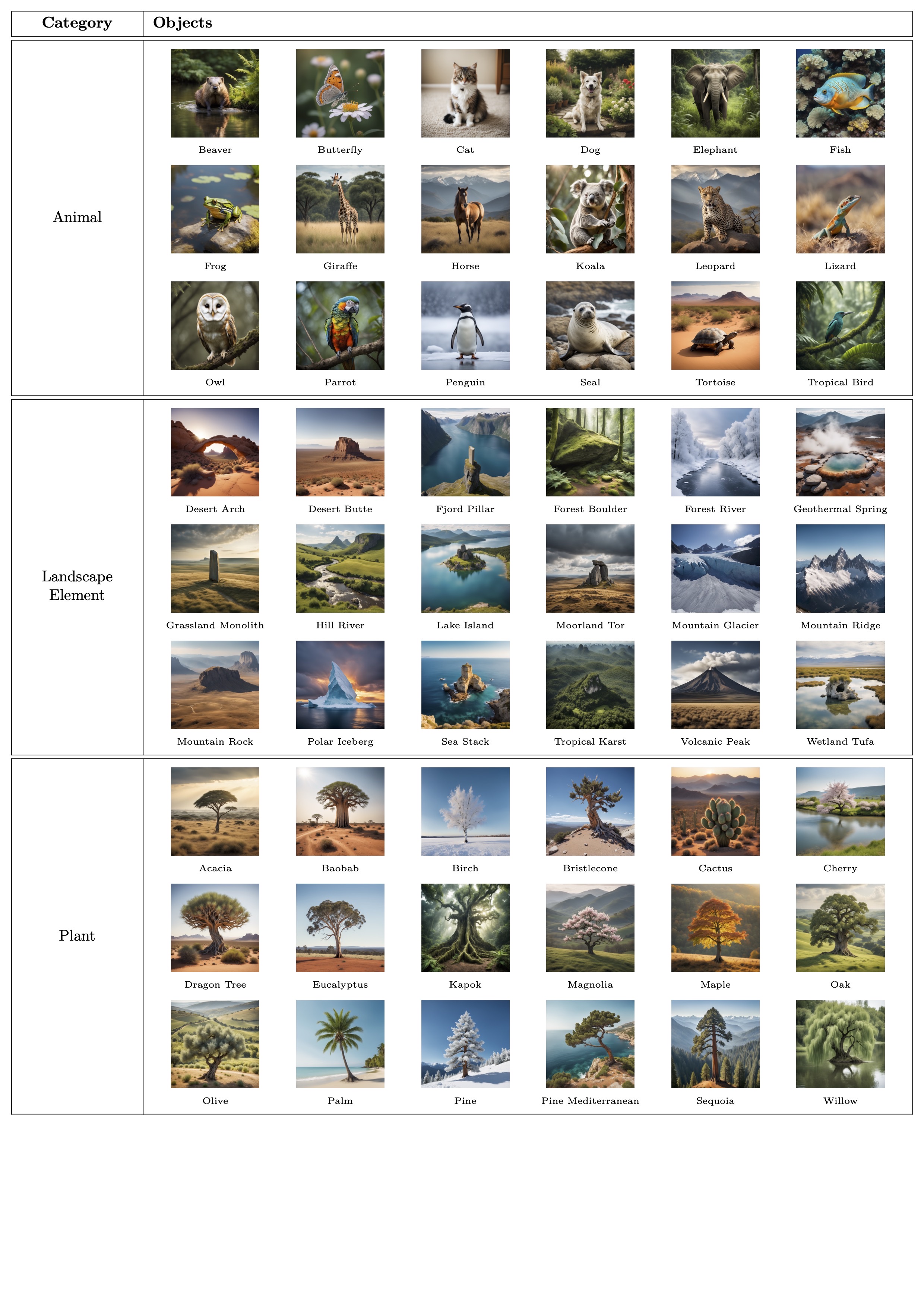
Figure 2: Table showing the categories and objects in the stimulus set. The categories in this table are classified as natural. For each object, the anchor image is shown.

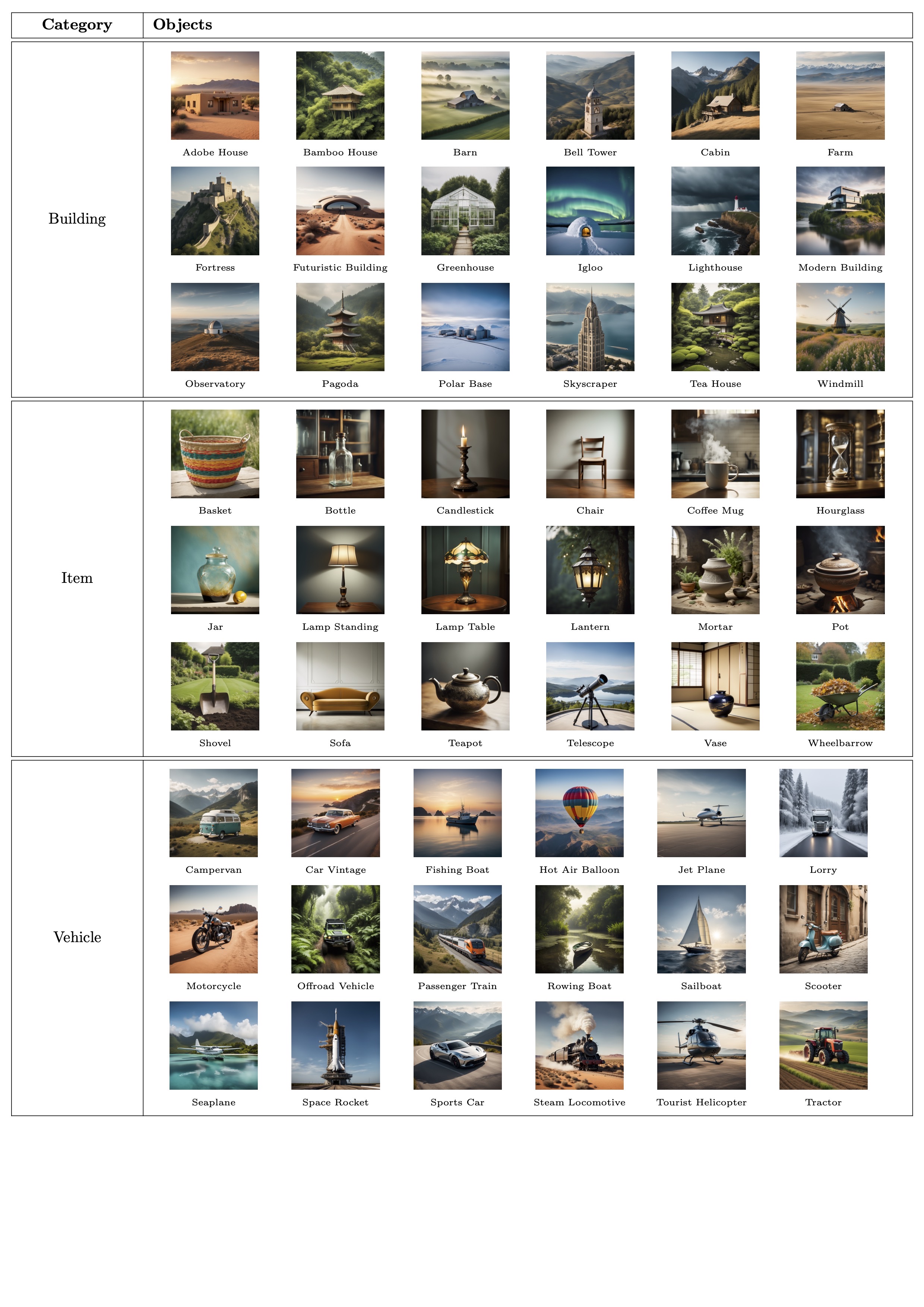
Figure 3: Table showing the categories and objects in the stimulus set. The categories in this table are classified as artificial. For each object, the anchor image is shown.

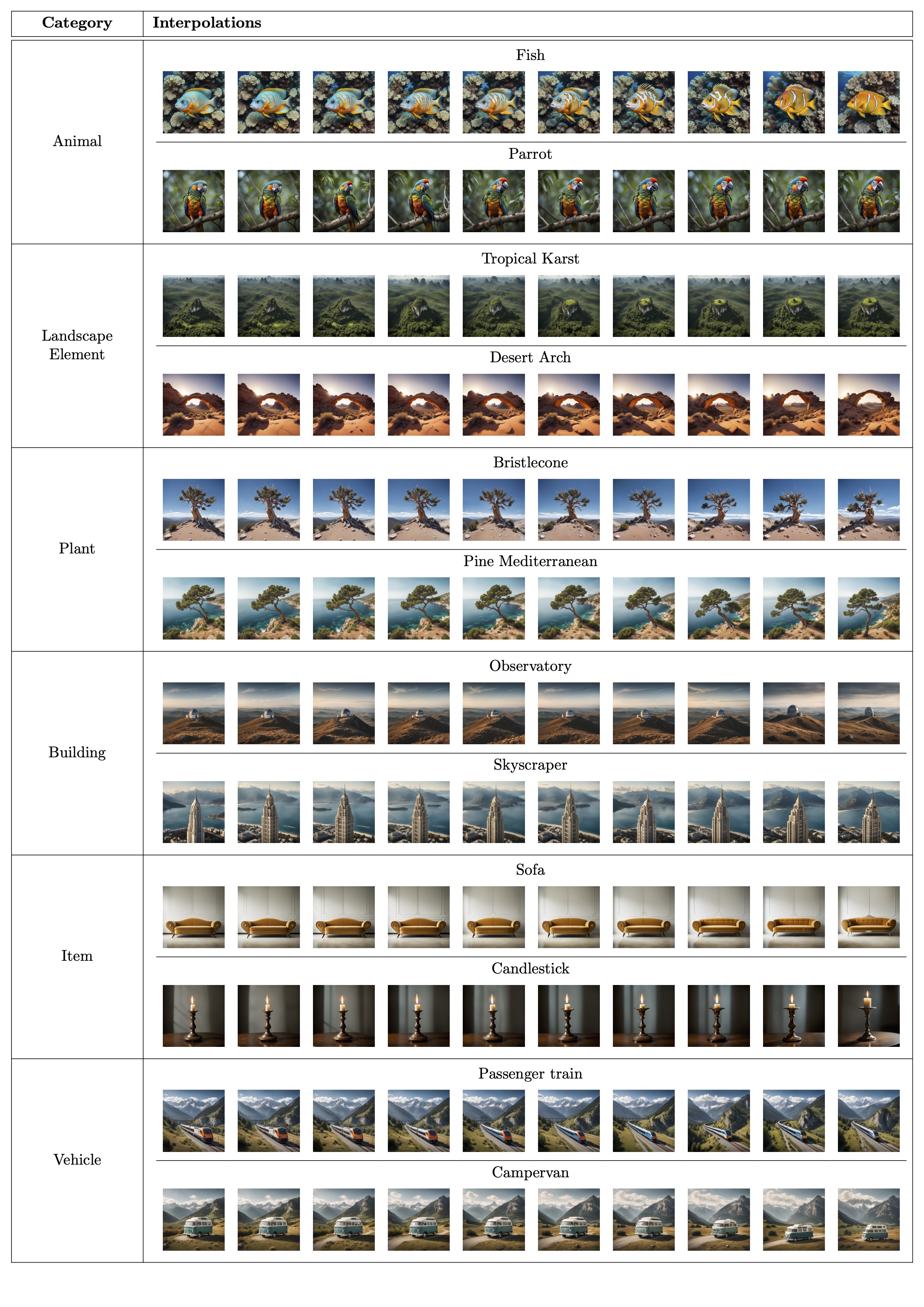
Figure 4: Examples of the final ordered image sets based on the psychophysical crowd-sourcing task. The figure shows the series for 2 out of 18 exemplars of each category. The anchor image is on the left.

4 Discussion

Our procedure synthesised a set of high resolution naturalistic object stimuli from different categories that are systematically ordered along a psychophysically validated perceptual continuum. They can thus be used for many cognitive tasks that involve measurements on perceptual continua, such as change detection or working memory tasks  [28]. In comparison to scraping images from the internet [11], or using pre-trained GANs [22], our text-to-image model in combination with psychophysical ordering also showed extreme versatility in semantic contents and high image quality.

There are nonetheless also limitations of our approach. For example, the overall categories and the specific objects (“butterfly”, “oak”) were decided “top-down”. Future work might combine systematic concept selection procedures with image synthesis to provide a thorough coverage of human semantic representations. As is common for AI-generated images we also identified artefacts, which exhibited high variability across categories. Although the exclusion rates were generally low, some objects were more prone to the presence of artefacts. This variability can be attributed to several factors. A first possibility is that there were differences in the availability of training data for different objects. Another possibility is the challenge of finding effective prompts, given the virtually infinite number of possibilities. Finally, the varying levels of familiarity with certain images, which may make artefacts more noticeable. The category with the highest incidence of artefacts was animals, followed by items and vehicles. For example, giraffe images had the highest exclusion rate, often due to inaccuracies such as an incorrect number of legs, which is a very salient feature. Also, there might be tighter normative constraints of features for certain objects, for example, the number of legs for a giraffe is fixed, whereas the number of leaves on a plant might be more variable. These are all known problems in generative AI, although models are quickly improving [40]. In contrast, artefacts were less frequent in images of plants, landscape elements, and buildings (which are less normatively constrained). Although investigating the causes of these differences was beyond the scope of this study, future research could examine this relationship experimentally, focusing on how humans perceive AI-generated images. A limitation of our approach is that the exclusion criteria were rather subjective and future work could use crowd-sourcing platforms to assess it more systematically.

The interpolation procedure successfully generated transitions between two selected images, producing a gradient of perceptual similarity without impacting the semantic meaning across image variations excessively. Keeping the text prompt constant while interpolating between the starting noise latents proved to be an effective and fairly controlled approach for maintaining the semantic meaning of a scene while manipulating its perceptual characteristics. However, generating smooth transitions was challenging, likely due to the non-linear nature of the high-dimensional space in which the interpolations were performed. Even though increasing the interpolation steps did make the transitions smoother, we occasionally observed perceptual “jumps” up to 1000 interpolation steps. However, visual inspection for artefacts revealed that most interpolated images maintained high quality, with 87.62% requiring no swaps. This might be an advantage in comparison to GANs, whose interpolations are smoother but also prone to artefacts. Objects with higher artefact prevalence during the initial generation, such as the giraffe and rowing boat, continued to show higher swap rates, suggesting consistent challenges in generating certain types of images.

The LPIPS metric [39] played a central role as a quantifiable prediction of perceptual similarity and enabled us to efficiently manage and screen a large set of images before fine-tuning the ordering based on psychophysics. In general, LPIPS showed a reasonable agreement with the similarity judgements from the online task and proved to be a valid first approximation. An open question is whether the LPIPS metric is affected by imperceptible patterns in the images, which are introduced by the diffusion process. One limitation of our approach is the absence of a comparable baseline similarity across object pairs. We found the score to be reliable and aligned with human perception within objects, whereas interpreting and comparing the scores across objects was more challenging.

5 Conclusion

The use of generative models for stimulus synthesis has the potential to set a new standard in cognitive research by enabling the creation of customised, naturalistic stimuli and psychometrically ordered stimuli tailored to the needs of cognitive experiments. These models can be of great help in tackling the trade-off between ecological validity and experimental control.

This study provides an approach for generating synthetic stimulus sets for cognitive research based on Stable Diffusion XL. By leveraging text-to-image synthesis, we create high-quality, photorealistic stimuli that vary along a perceptual scale while maintaining semantic consistency. These stimuli are particularly well-suited for addressing key challenges in visual cognitive research, including change detection, memory, and object recognition.

Data Availability

We will provide code, the stimulus set—including images and metadata—as well as the behavioral data from the online task upon request. These resources will be published on GitHub and OSF as soon as the article is accepted for publication.

Competing Interests

The authors declare no competing interests.

Appendix A Methods

In the next section, we provide detailed information about the model and its parameters. We will then describe the criteria used to generate exemplar images, followed by an explanation of how fine-grained image variations were obtained through interpolation between initial noise latents. A schematic overview of the procedure is shown in Figure 1.

A.1 Model

Text-to-image diffusion models such as Stable Diffusion [35] have gained considerable interest in the past years. They rely on two fundamental components to generate images: a starting noisy latent and a textual prompt. The noisy latent provides an initial random state, which the model progressively refines through a series of denoising steps, outputting an image. The textual prompt guides the model, conditioning the denoising process to generate images that align with the described content. Several text-to-image models are available on the market. We opted for Stable Diffusion XL (SDXL) [37] for two main reasons: output quality and customizability. In comparison to previous versions, SDXL relies on a larger UNet backbone and excels at generating high-quality images, especially at high resolutions (1024x1024 pixels). Moreover, the SDXL architecture incorporates two text encoders instead of one (OpenCLIP ViT-bigG and the original CLIP ViT-L text encoder), creating a richer textual conditioning for the diffusion process. Stable Diffusion XL benefits from a two-step generation process involving a base model and a refiner model, known as the ensemble of expert denoisers [41]: the base model generates a latent image, which is then fed into the refiner model. The refiner model completes the denoising process, enhancing the details of the image. In SDXL, the refiner model can be used to improve output quality of the fully-refined image. The base and refiner model pipelines were instantiated from pretrained model weights, which were downloaded from the Hugging Face repository. Images were generated using 50 inference steps for the base model to fully denoise the image and an additional 15 steps for the refiner model to improve detail quality. The default invisible watermark was added to each image to ensure it is marked as AI-generated. The ensemble of expert denoisers was integrated using a pre-trained Low-Rank Adaptation (LoRA) [42] model to further improve the quality and detail of the generated images. Unlike the refiner model, which improves detail quality through additional inference steps, LoRA modifies the base model weights by adding a low-rank update matrix, allowing for efficient fine-tuning.

We used the Hugging Face diffusers 0.26.02 Python library, alongside standard libraries such as PyTorch 2.0.1 [43], which provides high usability and customizability. We ran the model on the GPU cluster at the Bernstein Center for Computational Neuroscience, Charité-Universitätsmedizin Berlin, Germany. The cluster included four NVIDIA GeForce RTX 3090 GPUs (24GB each). To ensure efficient utilisation of the GPU resources, we distributed the image generation tasks across the available GPUs using Pytorch Multiprocessing. Each GPU processed a single image independently.

A.2 Generation pipeline: design and diffusion of exemplar images

Generating images from textual prompts has the unprecedented advantage of letting users create any possible composition using natural language, but it also presents the problem of how to narrow down the prompt space to generate a finite and usable number of stimuli. We established the following criteria to generate our stimuli: first, they should have a clear subject, situated in the centre and foreground (e.g. a picture of a cat sitting on the carpet); second, they should be situated in a coherent and realistic scene (e.g. an animal in its natural habitat); finally, there should be no human figures in the scenes.

Moreover, we divided the main subjects into six broad categories, three natural/living (“animals”, “plants”, “landscape elements”) and three artificial/non-living (“items”, “buildings”, “vehicles”). For each category, we defined a set of 18 objects (e.g. “cat”, “olive tree”, “sailboat”, “sofa” etc.), which we chose with the aim of creating a relatively diverse sample (e.g. animals from diverse biospheres, different kinds of landscape etc.). All categories and corresponding objects are listed in Table 1. For each object, we generated 60 exemplars using the same prompt, but varying the starting noise tensor.

The structure of textual prompts was designed to balance two main aspects. On the one hand, the resulting images should vary across categories and be rich in detail. On the other hand, the whole stimulus set should have some consistency in terms of image layout. Therefore, we used relatively specific prompts, but with a shared main structure across the sample. With few exceptions, prompts started with a declaring the main subject (e.g. “film solitary bristlecone pine” or “photo of a barn owl” ), followed by information about its position (e.g. “in the foreground”, “in the centre”) and about the background or scene it is situated in (e.g. “rocky terrain and blue sky in the background”), to finally describe the image style (“high resolution photography”) and some additional attributes (e.g. “cinematic”, “bright light”, “beautiful”). In order to avoid the undesired addition of human figures, we also used a negative prompt (“people, person, human figures, human body parts, humans”), which was constant across all generations. We checked that this worked as intended by visual inspection. Using this procedure, for each object we generated a set of 60 various but semantically homogenous exemplars, maintaining its layout and general composition fairly consistent.

We initialised the starting noise latents of each exemplar using unique seed values (for 60 exemplars and 108 objects, 6480 seeds in total). Seeds were used to create a PyTorch Gaussian noise tensor with dimensions (1, 4, 128, 128), where 128 is determined by dividing the target resolution (1024) by the Variational Autoencoder (VAE) scale factor of 8 used in Stable Diffusion XL. Storing the seeds ensured the reproducible initialization of the noise latents, making it possible to generate the same exact image at later stages of the pipeline, as well as to interpolate between noise latents.

After generation, we visually inspected all images and excluded those with prominent artefacts (such as an animal with too many legs), especially in central positions. The reason behind this is that they can be distracting and therefore make the stimulus less suitable for a cognitive scientific experiment. However, we will include these images in an extended stimulus set (see Data Availability section) for researchers who may be interested in using them for further studies, such as those focusing on human perception of AI-generated artifacts.

A.3 Image interpolations

A.3.1 Selection of the anchor images

In order to create variations of increasing dissimilarity from the exemplar image, we set up a procedure relying on the interpolation of the noise latents corresponding to a selected image pair. Each image pair included two anchor images, an anchor image and a guide image for the interpolation. These images were selected according to the following criteria:

1. The chosen images should be representative for the generated batch (e.g. no outliers).

2. They should be relatively similar to one another in terms of composition and perceptual features, avoiding changes in orientation or scene layout as much as possible.

Such criteria sought to optimise the interpolation smoothness (in the next step) while minimising our manual interference with the process. In order to satisfy both conditions, for each object we identified two images based on their relative perceptual similarity within the generated set. To quantify their perceptual similarity, we used the Learned Perceptual Image Patch Similarity (LPIPS) metric [39]. The LPIPS metric quantifies the perceptual differences between images by comparing deep features extracted from a pre-trained neural network and it has been shown to correlate well with human judgement. For a few test images, we compared metrics using features from the SqueezeNet [44], AlexNet [45], and VGG [46] architectures. The results across these models were comparable. Therefore, we opted to use SqueezeNet due to its computational efficiency and speed. We first computed the pairwise similarity of each image within the set. Then, for each image, we computed its mean LPIPS score against all other images in the set to assess its representativeness. The assumption behind this approach is that an image with a lower mean LPIPS score is, on average, more perceptually similar to the other images in the set. This higher similarity makes it a better representative of the overall set’s perceptual characteristics. The first image of the pair (the anchor image) was the image with the highest overall similarity to the rest of the set, that is, with the lowest mean LPIPS score. To select the guide image, we used the following procedure: first, we ranked images based on their mean LPIPS scores, and considered the images with the five lowest scores (excluding the score of the anchor image), which amounted to the top 8%-10% of the image set, depending on how many images had been excluded. We then ranked the images within this subset by their similarity with the anchor image, selected the most similar as the guide image and other ones as backup images. We then visually inspected the selected pairs. If the guide image had a significant visual disparity from the anchor image (e.g., opposite orientation), we selected the next most similar image as a backup. This process continued, if necessary, to the third most similar image and so forth, to ensure the pair maintained a high degree of perceptual coherence while maintaining the selection as objective as possible. In this way, we made sure that the interpolation would be computed between two images that are both representative of the set and similar to each other.

A.3.2 Interpolation algorithm

Once the two anchor images were selected, we generated the interpolations between the anchor and the guide image using their starting noise latents. In contrast to GANs, where the interpolation between two latent vectors corresponds to smooth image transitions, direct interpolation in diffusion is less straightforward. The interpolation between images can be operated either in the prompt space (i.e., between text embeddings), between the starting noise latents or both (Figure 5). Since the goal of this work was to maintain the semantic aspects of the images fairly constant, while changing their perceptual features, we interpolated between noise latents while maintaining the text embeddings constant. Spherical linear interpolation (slerp) is particularly suitable for interpolating high-dimensional data as it preserves the length of the vectors and ensures smooth transitions [47]. Given two vectors $\mathbf{v}_{0}$ and $\mathbf{v}_{1}$ and an interpolation parameter $t$ where $0\leq t\leq 1$, slerp can be defined as:

$$\text{Slerp}(\mathbf{v}_{0},\mathbf{v}_{1};t)=\frac{\sin[(1-t)\theta]}{\sin[\theta]}\mathbf{v}_{0}+\frac{\sin[t\theta]}{\sin\theta}\mathbf{v}_{1}$$

where $\theta$ is the angle between $\mathbf{v}_{0}$ and $\mathbf{v}_{1}$, determined using the arccosine function on the normalized dot product between the vectors:

$$\theta=\arccos\left(\frac{\mathbf{v}_{0}\cdot\mathbf{v}_{1}}{\|\mathbf{v}_{0}\|\|\mathbf{v}_{1}\|}\right)$$

We first defined 200 interpolation values $t$ or “steps”, which are linearly spaced between 0 and 1. The number of interpolation steps determines the granularity of this transition. We chose 200 steps as a compromise to balance between computational time and smoothness of transition. Feeding the interpolation steps in the slerp function, we generated a series of intermediate noise latents that transition between the noise latents that were used to synthesize the anchor image and the guide image. We then used SDXL to denoise each interpolated latent and generate intermediate images. Importantly, we diffused the images iteratively in two sequential batches. In the first batch, we used the PyTorch generator initialised with the seed from the anchor image and diffused each intermediate noise tensor up to the midpoint. In the second batch, we used the PyTorch generator initialised with the seed from the guide image and diffused each intermediate noise tensor back to the midpoint. This dual-batch approach helped mitigate small variations or inconsistencies in the final output images, making sure that the diffusion process was equally controlled by both seeds.

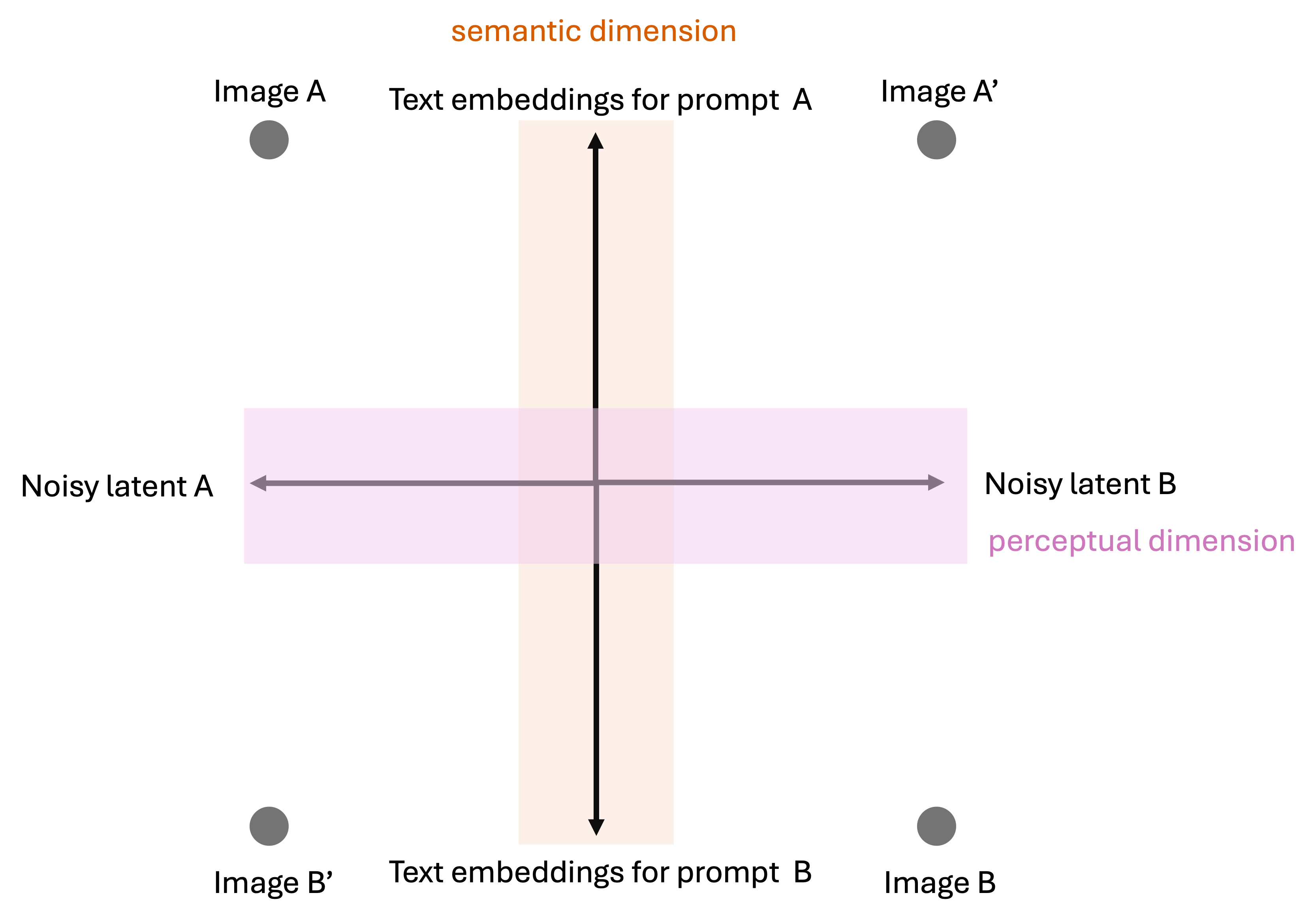
(a)

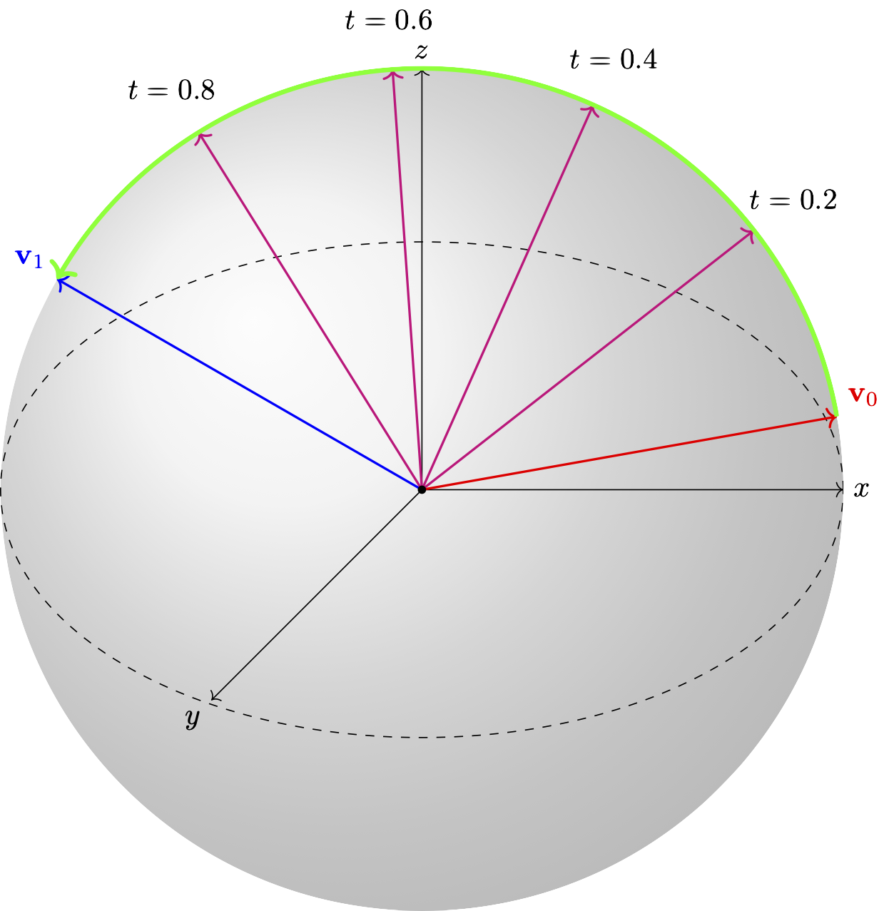
(b)

Figure 5: a) Schematic representation of the two possible spaces in which the interpolation can be operated. It is possible to interpolate either between the text embeddings (encoded by the CLIP models) or the initial noisy latents. Interpolation between text embeddings will result in significant semantic variations (e.g. between Image A and Image B, or B’), whereas interpolations between noisy latents will mostly involve perceptual variations, keeping the meaning of the image fairly constant (e.g. between Image A and A’ or Image B and B’). It should be noted that this is a simplification because semantic variations cause perceptual variations and vice versa. The aim here is to highlight the main dimension of variation. Moreover, to have fine-grained control of the scene layout, methods relying on models like ControlNet should be used. b) A three-dimensional simplification of the spherical linear interpolation (slerp) between two vectors $v_{0}$ and $v_{1}$. In this study, the interpolation is applied between $128\times 128\times 4\times 1$ tensors.

A.3.3 Selection of the interpolated images

For each object, we selected ten variations, the anchor image and nine of its interpolations. To do so, we again used the LPIPS metric to compute the perceptual similarity between the anchor image and every interpolated image. We defined target similarity scores, linearly spaced between the minimum and maximum LPIPS values observed. For each target score, we selected the image whose similarity score was closest to the target score, ensuring the absence of duplicates. This involves calculating the absolute differences between the similarity scores and the target scores, and selecting the closest matches. One option could have been defining the variations in terms of interpolation steps (e.g. generating 10 interpolation steps in the previous step). Our approach, however, presents two advantages. First, the interpolation process in high-dimensional latent spaces can result in complex, non-linear changes in perceptual similarity. Consequently, simply selecting images based on fixed intervals of interpolation steps might not accurately represent a linear increase in dissimilarity from the anchor image. Our approach thus partially compensates for the non-linear perceptual changes by focusing on the actual observed similarities, rather than the potentially misleading interpolation steps. Secondly, the image generation process is susceptible to the introduction of artefacts. Since we wanted to make sure that the final image set maintained a high quality and, at the same time, a perceptual gradient, we conducted a final visual inspection to identify and exclude images with noticeable artefacts. If artefacts were detected, we selected immediate neighbours with very similar LPIPS scores as replacements. Therefore, generating a large number of interpolated images allowed us to exclude interpolated images with significant artefacts in favour of neighbouring images, without affecting the perceptual gradient significantly and minimising the interference of our own subjective judgement.

A.4 Similarity ratings from human participants

We used the LPIPS metric to pre-select ten images per object because it aligns reasonably well with human perceptual judgment [39], and having participants evaluate all 108 objects with 200 images each would have been experimentally challenging. Although LPIPS provides a good approximation, we conducted a crowdsourcing task to experimentally validate the pre-selected images and adjust their ordinal positioning if needed.

A.4.1 Participants

We recruited 1286 participants from the online platform Prolific, with a remuneration of 8.53 GBP ($\sim$10 EUR) per hour. The sample of recruited participants was larger than the target minimum sample size (at least 20 participants judging an object, for a total 1080), because we anticipated that we might have to exclude up to 20% of data as has been reported previously for online experiments [48, 49]. Participants were selected from a standard sample, aged between 18 and 40 years, fluent in English, and with an approval rate on the platform of 100%, to maximise data quality. All participants provided informed consent before taking part in the study. The consent process included detailed information about the purpose and duration of the experiment, voluntariness of participation, and data protection policies. The study was approved by the Ethics Committee of the Institute of Psychology of the Humboldt University Berlin, Germany.

A.4.2 Stimuli

The final stimulus set included a total of 1,080 images, comprising 18 objects from 6 categories, with 10 variations per object (see above for the selection procedure). Images were handled in PNG format and downscaled to 512x512 to decrease potential latencies from the client side, while maintaining high quality.

A.4.3 Similarity judgement task using triplet comparisons

Participants performed a similarity judgement task based on triplet comparisons, or “method of triads” [50], which is used both in psychophysics and machine learning [51, 52, 53, 54, 55, 56]. Given a set of stimuli $S=\{s_{1},s_{2},\ldots,s_{n}\}$, where $n$ is the total number of stimuli, participants are asked to judge the similarity of three stimuli at a time. In particular, given a triplet of stimuli $(s_{i},s_{j},s_{k})$, they are asked which between two probe stimuli $s_{j}$ and $s_{k}$ is most similar to a reference stimulus $s_{i}$. From the set of stimuli $S$, the number of all possible unique triplets is determined by the binomial coefficient:

$$\binom{n}{3}=\frac{n!}{3!(n-3)!}$$

However, since each element of the triplet can be a reference stimulus, the total number of possible triplet questions is obtained by multiplying the binomial coefficient by three:

$$C=3\cdot\binom{n}{3}$$

Since we planned to let participants assess the similarity between each combination of variations of the same object, but not across objects, in our case $n$ was 10 (total number of image variations for each object) and the total number of triplet combinations $C$ was 360.

Prior to data collection, we ran a set of simulations to estimate a) the number of triplet judgements that we would need to estimate object-specific psychophysical similarity functions robustly, and b) a target sample size of participants to judge each object. Previous work has shown that for $n$ objects and $d$ perceptual embedding dimensions, a subset of $2dn\log(n)$ triplets should be sufficient to reconstruct the embeddings with small error [53, 57, 58], which for $n=10$ and $d=1$ amounts to $2\cdot 1\cdot 10\log(10)=20\log(10)\approx 46$ triplets. Following the simulation results and expecting a relatively high noise for naturalistic images that are perceptually very similar, we estimated that a subset of 144 triplet judgements for one object from each single participant (40% of the total possible triplet combinations $C$) and at least 20 participants for each object would be necessary. The subset of triplet combinations was randomly sampled for each participant independently. Because of experimental constraints, i.e. not making the online task too long, each participant was assigned two objects. The assignment of the objects to participants was randomised.

A.4.4 Task procedure

After providing informed consent, participants received detailed instructions on the task procedure and had to pass an attention check to make sure they understood the instructions. Before starting the main task, they underwent a training session where they performed 12 trials using an independent set of stimuli. The main task consisted of 288 trials divided in 6 blocks of 48 trials each. In between blocks, participants were prompted to take a short break (maximum 2-3 minutes) to maintain attention and accuracy. Each trial began with a fixation target [59] presented at the centre of the screen for a jittered duration between 500 and 1000 ms, which was randomized in 100 ms steps. Then, participants were shown three images: one reference image on top and two probe images below (see Figure 6). Their task was to judge which of the two probe images was more similar to the reference image. Participants made their choices by pressing the “f” and “j” keys to select, respectively, the left or the right probe. They were asked to respond within 5 seconds and – if they did not – after their response they were prompted to respond more quickly. The opacity of the selected image was reduced to 0.5 for 1000 ms, giving participants visual feedback that their response had been registered. At the end of the experiment, participants were given the option to complete a debriefing questionnaire about their experience. They were asked for their overall impressions of the study, whether they encountered any technical problems, if they used any specific strategies during the experiment, and for any additional feedback they might have.

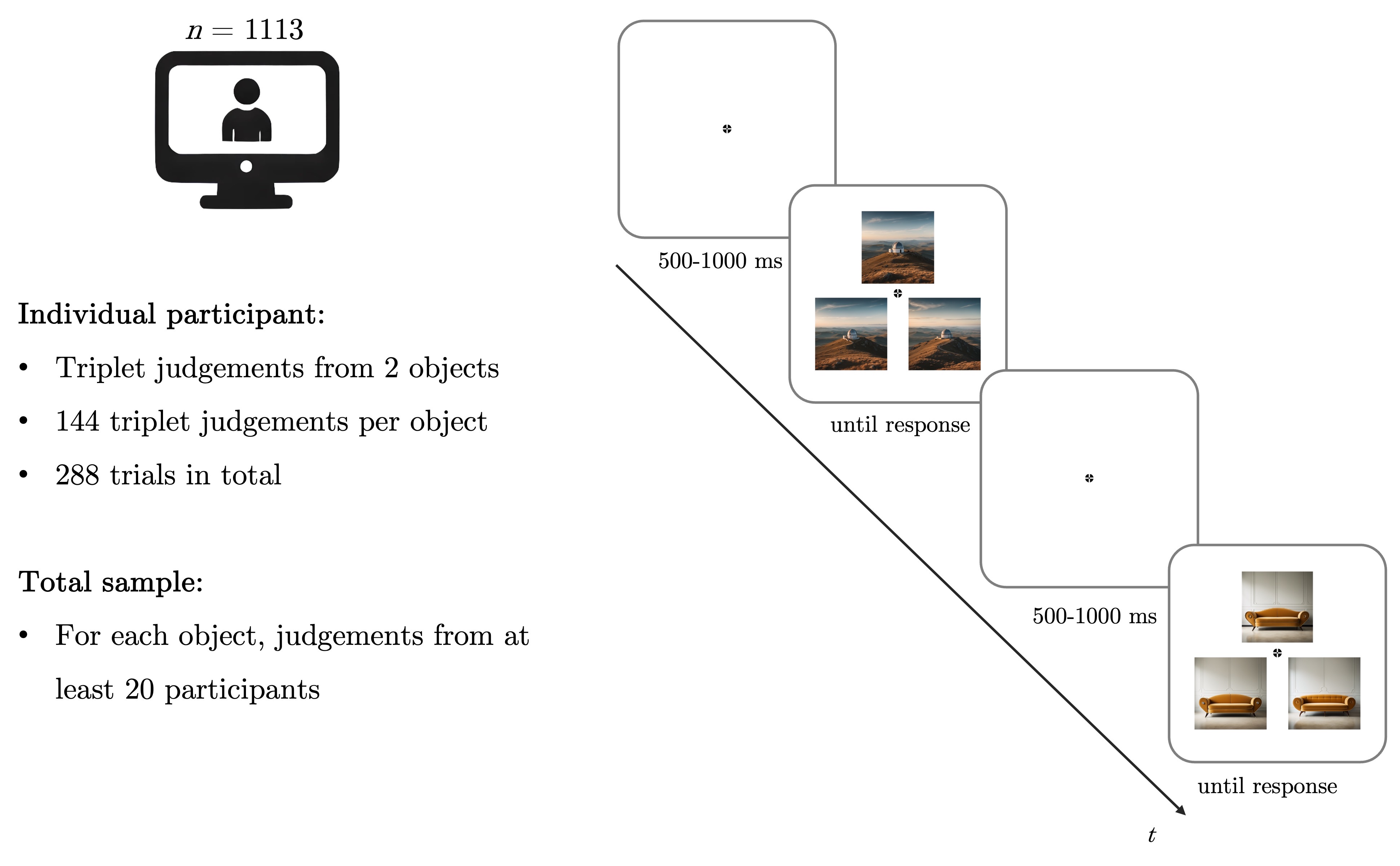
Figure 6: Online task design with two example trials of the similarity judgement task (for observatory and sofa). Participants were tasked to indicate which of the two bottom images is most similar to the top image. Each participant was assigned two objects and the triplet comparisons were always between variations of the same object.

A.4.5 Experimental control, data quality, and exclusion criteria

A key drawback of online studies compared to on-site experiments is the lack of experimental control, but there are several strategies to maintain data quality [60]. We implemented both experimental measures during data collection and an analysis pipeline with sanity checks on the collected data. In order to ensure a relative consistency in the experimental environment, participants were required to use a desktop device, the Google Chrome web browser with a minimum screen resolution of 800x600 pixels and to remain in fullscreen mode throughout the experiment. These requirements were enforced through a preliminary device and browser check before the experiment began and by pausing the experiment if participants exited fullscreen mode. Every interaction with the browser (e.g. if participant exited fullscreen) was recorded, in addition to the time spent in each phase of the task (e.g. how much time they spent on each break). Such data was crucially important to identify and potentially exclude participants who showed unreliable engagement with the experiment. Participants who did not finish the experiment were also excluded. In addition to the interaction data, we used two behavioural indicators to flag participants with outlying performance: reaction times and response biases. We first examined the distribution of RTs (Figure 7) and identified these outliers with very short RTs. Any participant with mean RTs below 1000 milliseconds was excluded, assuming that a mean RT below 1000 ms throughout the task would indicate that a participant might have performed the task inattentively. We also examined the distribution of response biases (Figure 8), making the assumption that participants who pressed one of the two keys with high frequency were not fully engaging with the task. We first calculated the proportion of choices for ‘f’ (left probe) and ‘j’ (right probe) key presses for each participant, to then exclude participants with biases falling 1.85 times outside the interquartile range bounds. Finally, we conducted an analysis of participant feedback provided at the end of the experiment to identify potential technical problems or other issues encountered during the study.

Of 1253 participants who participated in the experiment, 140 (11%) were excluded either because they did not complete all trials (92 participants, 7.3%) or because they did not satisfy the inclusion criteria based on reaction times (36 participants, 2.9%) and response biases (20 participants, 1.6%), with 4 (0.3%) participants satisfying more than one exclusion criterion. A final sample of 1113 participants passed the criteria and was used for the analysis. The final sample had an average age of 28.9 years (SD = 5.7). The majority of participants were male, accounting for 60% of the sample, while 39.6% were female. A small proportion, 0.4%, chose not to disclose their gender. Each participant provided judgements only for two objects and each object was assigned to at least 20 participants. The majority of objects (56) were judged by 20 participants, 38 objects were judged by 21 participants, and 14 objects were judged by 22 participants (Figure 9 and Table LABEL:tab:participant_count_for_objects). Because of the very small difference, we included all data in the final analysis.

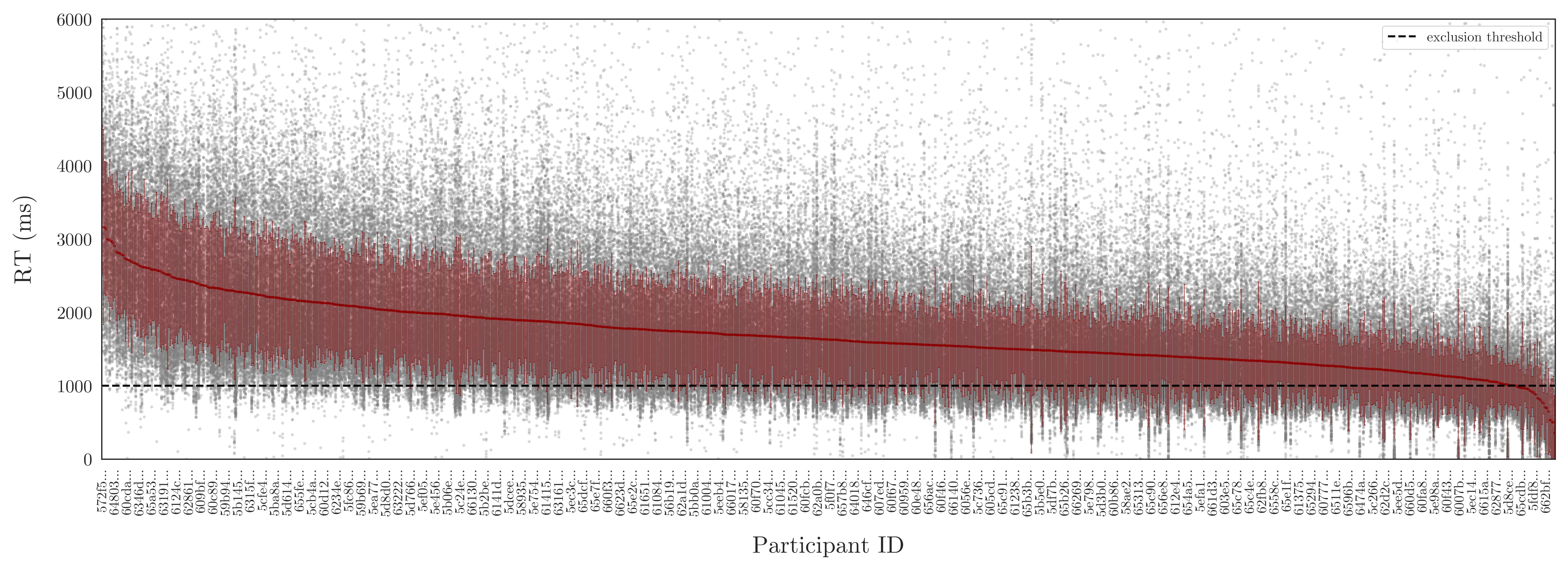
Figure 7: Distribution of reaction times for all participants, ordered by mean reaction time. The 1000 ms cutoff threshold is indicated by the dashed line.

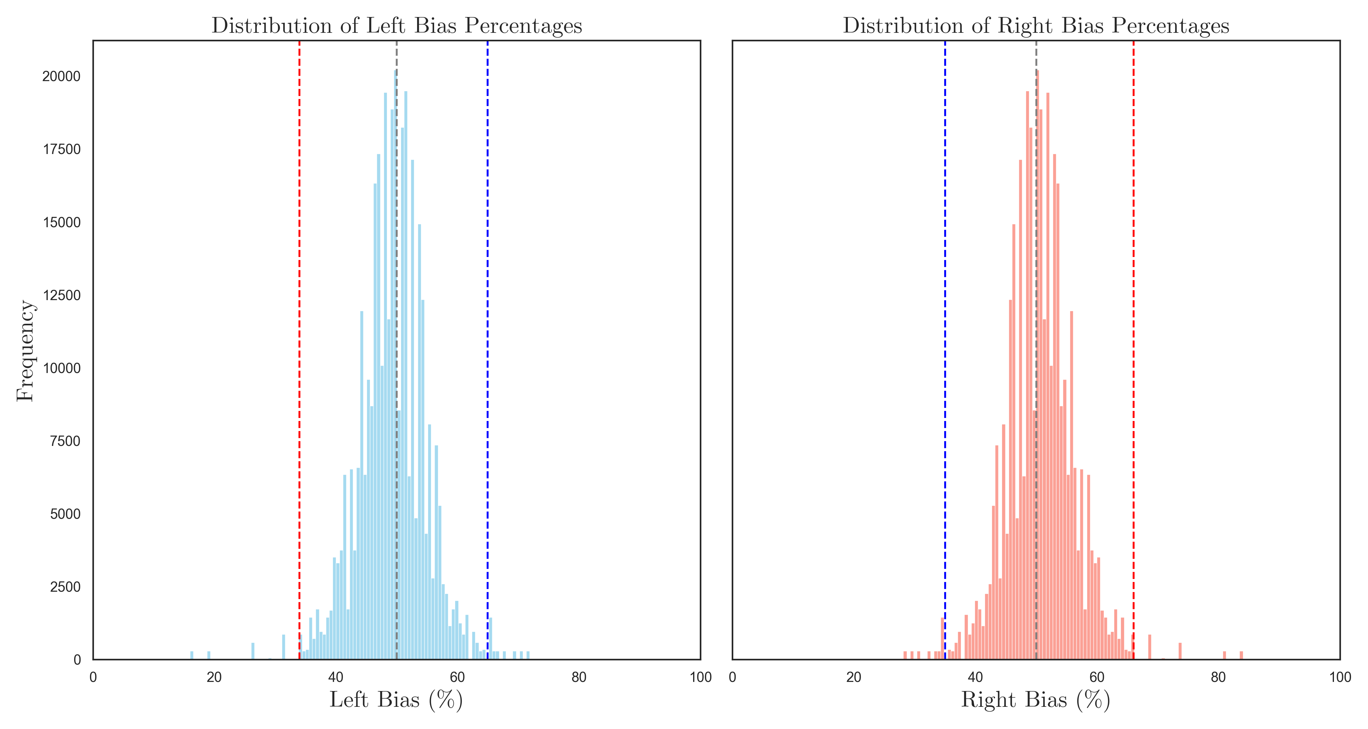
Figure 8: Distribution of left and right bias percentages across participants. The dashed blue and red lines indicate the thresholds for extreme biases, while the central black dashed line represents the expected 50% bias.

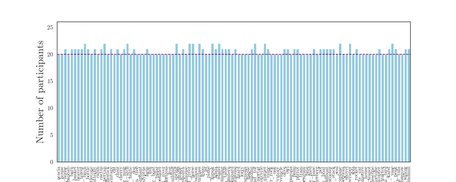
Figure 9: Participant count for each object.

Table 2: Number of participants assigned to each object.

object name	number of participants assigned
acacia	20
adobe_house	20
bamboo_house	21
baobab	20
barn	21
basket	21
beaver	21
bell_tower	21
birch	22
bottle	21
bristlecone	20
butterfly	21
cabin	20
cactus	21
campervan	22
candlestick	20
car_vintage	21
cat	20
chair	21
cherry	20
coffee_mug	21
desert_arch	22
desert_butte	20
dog	21
dragon_tree	20
elephant	20
eucalyptus	20
farm	21
fish	20
fishing_boat	20
fjord_pillar	20
forest_boulder	20
forest_river	20
fortress	20
frog	20
futuristic_building	20
geothermal_spring	22
giraffe	20
grassland_monolith	21
greenhouse	20
hill_river	22
horse	22
hot_air_balloon	20
hourglass	22
igloo	21
jar	20
jet_plane	20
kapok	22
koala	21
lake_island	22
lamp_standing	21
lamp_table	21
lantern	21
leopard	20
lighthouse	21
lizard	20
lorry	20
magnolia	20
maple	20
modern_building	21
moorland_tor	22
mortar	20
motorcycle	20
mountain_glacier	22
mountain_ridge	21
mountain_rock	20
oak	20
observatory	20
offroad_vehicle	20
olive	21
owl	21
pagoda	20
palm	21
parrot	21
passenger_train	20
penguin	20
pine	20
pine_med	20
polar_base	21
polar_iceberg	20
pot	21
rowing_boat	21
sailboat	21
scooter	21
sea_stack	21
seal	20
seaplane	22
sequoia	20
shovel	20
skyscraper	22
sofa	20
space_rocket	21
sports_car	20
steam_locomotive	20
tea_house	20
teapot	20
telescope	20
tortoise	20
tourist_helicopter	21
tractor	20
tropical_bird	20
tropical_karst	21
vase	22
volcanic_peak	21
wetland_tufa	20
wheelbarrow	20
willow	21
windmill	21

A.4.6 Similarity judgement analysis

The main goal of the similarity judgement analysis was to estimate a perceptual scale for each object and its variations, given a set of perceptual judgements. To analyse the triplet judgements, we used three algorithms: Maximum Likelihood Difference Scaling (MLDS) [61], which is well-established scaling method in psychophysics, and two ordinal embedding algorithms, Soft Ordinal Embedding (SOE) [62] and t-Distributed Stochastic Triplet Embedding (t-STE) [63]. MLDS can be used only in one-dimensional cases, whereas t-STE and SOE have been proposed to find ordinal embeddings in higher dimensional spaces [53]. Embeddings, in this context, are Euclidean representations that preserve the ordinal relationships among data points based on a set of perceptual triplet judgments [64, 57]. Given a set of triplet constraints $\mathcal{T}=\{(i,j,k)\}$, derived from perceptual judgments where each triplet $(i,j,k)$ indicates that image $i$ is perceived as more similar to image $j$ than to image $k$, an embedding is a set of points $\{x_{i}\in\mathbb{R}^{d}\}$, where $d$ denotes the dimensionality of the embedding space, such that:

$$\|x_{i}-x_{j}\|<\|x_{i}-x_{k}\|,\quad\forall\,(i,j,k)\in\mathcal{T}.$$

Because perceptual judgments are noisy and have inconsistencies, it may not be possible to satisfy all triplet constraints at the same time. For this reason, the embedding $\{x_{i}\in\mathbb{R}^{d}\}$ is obtained by solving an optimization problem that minimizes a loss function over the set of triplet constraints [64, 57].

We performed a comparative analysis between the three algorithms, assessing both their performance and the stability of the embedding estimates. To assess their performance, we used the cross-validated triplet error $E_{t}$ [53]. Given a set of embedding representations $y_{1},\ldots,y_{n}$ estimated on a triplet set $T$, the triplet error measures how many triplets from a validation set $T^{\prime}$ are not correctly represented by those embeddings. It is defined as follows [53]:

$$E_{t}=\frac{1}{|T^{\prime}|}\sum_{t=(i,j,k)\in T^{\prime}}\mathds{1}\{R_{t}\cdot\text{sgn}(\|\hat{y}_{i}-\hat{y}_{k}\|^{2}-\|\hat{y}_{i}-\hat{y}_{j}\|^{2})=1\},$$

where $\mathds{1}$ is the indicator function that equals 1 if the given triplet does not satisfy the expected distances and equals 0 if the relationship is satisfied. The triplet error thus counts the number of violations where the distance between the reference point $i$ and point $k$ is less than or equal to the distance between the reference point $i$ and point $j$. We used a Leave-One-Participant-Out cross-validation to evaluate embeddings for each object using the three different estimators. First, the triplet judgement data were grouped by object. For each object group, we divided the triplet judgements into training and test data. In each fold of the cross-validation, data from one participant were left out as the test set $T^{\prime}$, while the data from the remaining participants constituted the training set $T$. This ensured that the model was evaluated on data from a participant it had not seen during training, providing an unbiased estimate of its performance. Moreover, it also provided information about how generalisable the embedding estimates were across participants. For each fold of the cross-validation, we ran 10 iterations of the embedding estimation procedure for the t-STE and SOE algorithms. These methods, which rely on stochastic optimisation techniques like gradient descent, are prone to converging on local optima. To mitigate this, we ran the algorithm with multiple initializations and selected the embedding solutions that best fit the data, using the triplet error (calculated on the training set only) as the metric [53]. This approach increases the likelihood of identifying a more globally optimal solution by sampling various potential embeddings and reducing the impact of any single suboptimal result. Unlike t-STE and SOE, which often require multiple runs to achieve stable results, MLDS uses a maximum likelihood estimation approach that does not require multiple independent runs. Importantly, in each iteration the training data was used both to compute the embeddings and to calculate the triplet error to prevent data leakage. After running 10 iterations, we selected the embedding with the lowest triplet error as best fitting.

When the embeddings are computed, the scale and orientation of the solutions can vary across different iterations, resulting in inconsistencies such as varying scales and mirror images. To achieve a consistent scale and orientation, the embedding values were subjected to two transformations. First, we normalized them to the [0,1] interval. Second, we standardized the direction of the embeddings by enforcing a descending order using the Theil-Sen estimator [65, 66]. The estimator fits a line by calculating the median slope from all pairwise slopes of the data points within a sample, providing a robust measure of the general trend of the data. If the slope of the fitted line was positive, indicating an ascending order, we flipped and translated the embeddings $(1-y)$ to achieve the desired descending orientation within the [0,1] interval. Importantly, this method does not affect the triplet error calculation, since the relative distances are preserved. This method is suitable for our use case, which involves aligning the embeddings on a one-dimensional scale. For multidimensional embeddings, Generalized Procrustes Analysis or unsupervised methods [67, 68].

For each object and category, we calculated the mean cross-validated triplet error of each algorithm by averaging the triplet errors from all cross-validation steps. The object-wise and category-wise error estimated how well the model performed for individual objects and for categories. We also calculated the overall mean triplet error for each algorithm, which provided a general measure of how they performed across objects.

As a final step, we reordered the images according to the embedding results and compared this order to the one defined by the LPIPS metric.

A.4.7 Physical characteristics of the stimulus set

We calculated the physical characteristics of the stimulus set. These measures were calculated only for the anchor images. When necessary, color images were converted to grayscale using the OpenCV cvtColor function with the COLOR_RGB2GRAY conversion code. This function implements a color space conversion applying the following weighted sum of the RGB channels [69]:

$$\text{gray\_image}=0.299\cdot R+0.587\cdot G+0.114\cdot B$$

We calculated the following measures:

• Contrast: Defined as the standard deviation of the pixel intensity values in the normalized grayscale image. This measure captures the variation in intensity within the image and indicates the overall variability in brightness:

  $$\text{contrast}=\sqrt{\frac{1}{N}\sum_{i=1}^{N}\left(\frac{\text{gray\_image}(i)}{255.0}-\mu\right)^{2}}$$

  where $N$ is the total number of pixels, $\text{gray\_image}(i)$ is the intensity of the $i$-th pixel, and $\mu$ is the mean intensity of the normalized grayscale image:

  $$\mu=\frac{1}{N}\sum_{i=1}^{N}\frac{\text{gray\_image}(i)}{255.0}$$

  Normalizing by 255, which is the maximum intensity value for an 8-bit grayscale image, scales the pixel intensity values to a range between 0 and 1 and allows for consistent contrast evaluation across different images.

• Mean intensity: Calculated as the mean pixel intensity of the normalized grayscale image. The luminance was calculated using the formula:

  $$\text{mean\_intensity}=\frac{1}{N}\sum_{i=1}^{N}\text{gray\_image}(i)$$

  where $N$ is the total number of pixels and $\text{gray\_image}(i)$ is the intensity of the $i$-th pixel.

• Relative Luminance: Relative luminance takes into account the perception of brightness by considering the different sensitivities of the human eye to red, green, and blue light [70]. Calculated by first converting gamma-compressed RGB values to linear RGB values using a 2.2 power curve:

  $$R_{\text{lin}}=R^{\prime 2.2},\quad G_{\text{lin}}=G^{\prime 2.2},\quad B_{\text{lin}}=B^{\prime 2.2}$$

  Then applying the relative luminance formula according to the BT.709 standard [70]:

  $$Y=0.2126\cdot R_{\text{lin}}+0.7152\cdot G_{\text{lin}}+0.0722\cdot B_{\text{lin}}$$

• Colorfulness: The method for calculating image colorfulness is based on the approach by Hasler and Süsstrunk [71]. This method uses an opponent color space to quantify colorfulness and they show it correlates with human perceptual judgements. Two channels, $rg$ and $yb$, represent the differences between the red and green channels, and a combination of the red, green, and blue channels, respectively. These channels are computed as follows:

  $$rg=R-G$$

  $$yb=0.5\cdot(R+G)-B$$

  The mean ($\mu$) and standard deviation ($\sigma$) for these channels are calculated as:

  $$\sigma_{rgyb}=\sqrt{\sigma_{rg}^{2}+\sigma_{yb}^{2}}$$

  $$\mu_{rgyb}=\sqrt{\mu_{rg}^{2}+\mu_{yb}^{2}}$$

  The colorfulness metric is then defined as:

  $$\hat{M}(3)=\sigma_{rgyb}+0.3\cdot\mu_{rgyb}$$

  Here, $\sigma_{rgyb}$ combines the variability of the $rg$ and $yb$ channels, while $\mu_{rgyb}$ represents their combined mean value, adjusted by a factor of 0.3.

• Shannon Entropy: Entropy measures the amount of information or randomness in an image by analyzing the distribution of pixel intensity values. Higher entropy indicates more complexity and variation in pixel intensity values and reflects richness of detail in the image. It was computed using Shannon’s formula [72]:

  $$S=-\sum p_{k}\log(p_{k}),$$

  where $p_{k}$ represents the probability of a pixel having intensity value $k$, calculated from the frequency of each intensity value. $S$ quantifies how unpredictable the pixel intensities are within the image. This calculation was performed using the skimage.measure.shannon_entropy function from the scikit-image 0.24.0 package.

• Edge Density: Edge density is defined as the proportion of edge pixels to the number of pixels in a portion of the image [73]. This measure indicates the amount of structural detail present, with higher edge density suggesting more edges and thus more complexity [74]. Edge density was calculated using the Canny edge detection algorithm [75] and considering all pixels within the image. The Canny algorithm identifies areas of steep intensity change through a multi-stage process and outputs a binary map where edge pixels are marked. The formula for edge density is given by:

  $$\text{edge\_density}=\frac{N_{\text{edge}}}{W\times H}$$

  • $N_{\text{edge}}$ is the number of edge pixels identified by the Canny edge detection algorithm.

  • $W$ is the width of the image.

  • $H$ is the height of the image.

  The algorithm was implemented using the feature.canny function from scikit-image 0.24.0.

• Blur Strength: Blur strength estimates the amount of blurring present in an image. It was calculated using the skimage.measure.blur_effect function, based on the method described by Crete-Roffet et al. [76], which developed a perceptual blur metric that correlates well with human perception of blur and has been validated through subjective tests.

• Sharpness: Sharpness measures the clarity of edges and fine details in an image. To quantify sharpness, we follow the method outlined by [77], which relies on a Laplacian operator detecting regions of rapid intensity change (edges) by computing the second spatial derivative of the image. The sharpness metric, $\text{LAP\_VAR}(I)$, is defined as the variance of the Laplacian values.

  First, a Laplacian mask is applied to the image to compute the Laplacian values $L(m,n)$ at each pixel $(m,n)$. The mask is:

  $$\text{laplacian\_mask}=\begin{bmatrix}0&-1&0\\ -1&4&-1\\ 0&-1&0\end{bmatrix}$$

  This operation enhances the edges by emphasizing regions where there is a significant change in intensity.

  Next, the mean of these absolute Laplacian values, $\bar{L}$, is calculated as follows:

  $$\bar{L}=\frac{1}{NM}\sum_{m=1}^{M}\sum_{n=1}^{N}|L(m,n)|$$

  where $M$ and $N$ are the dimensions of the image, and $|L(m,n)|$ represents the absolute value of the Laplacian at pixel $(m,n)$.

  The sharpness metric, $\text{LAP\_VAR}(I)$, is then computed as the variance of these Laplacian values around the mean:

  $$\text{LAP\_VAR}(I)=\sum_{m=1}^{M}\sum_{n=1}^{N}\left(|L(m,n)|-\bar{L}\right)^{2}$$

  In this formula:

  • $L(m,n)$ is the Laplacian value at the pixel $(m,n)$.

  • $\bar{L}$ is the mean of the absolute Laplacian values.

  High variance in these values indicates a sharp image with well-defined edges, whereas low variance suggests a blurred image with less distinct edges.

• Spectral energy: Image statistics vary depending on scene content and viewing conditions [78]. Second-order statistics such as the power spectrum, which describe the relationships between pixel intensities, are strongly correlated with scene scale (the spatial extent and distance of scene elements) and scene category (e.g., natural or man-made environments). Analyzing the spectral energy of images helps in understanding low-level features of the stimuli [23]. Using the Natural Image Statistical Toolbox for MATLAB [79], adapted for Python, we measured the spectral characteristics of each image. We determined the dominant spatial frequencies by finding the frequency below which 80% of the total spectral energy is contained. We also assessed high spatial frequencies by calculating the proportion of frequencies above 10 cycles per image. Such metric quantifies the amount of fine details and textures within the image.

A.4.8 Programming tools

The experiment was implemented using the jsPsych library 7.3.1 [80] and JATOS [81], which was installed on a server at the Bernstein Center for Computational Neuroscience (Berlin, Germany). Experimental condition assignments were managed via an external database and a backend application using Python FastAPI 0.111.0, hosted on Vercel. To run the embedding analyses, we used the Python package cblearn [82], as well as the original MATLAB code for t-STE and the original R code for MLDS [83] for replication tests. Since we could successfully replicate the results, we report only the final results obtained using the cblearn package.

Appendix B Supplementary Results

B.1 Image Generation

B.1.1 Exemplar images

We generated 60 exemplar images for each one of the 108 objects, for a total of 6480 images. The synthesised images were visually evaluated for their quality and fidelity to the input textual prompts, which was generally high. The application of the LoRA model visibly enhanced the quality of the generated images, especially making contrast and scene lighting more realistic.

After visual inspection, 215/6480 images (3.3%) were excluded (Figure 11). We provide some examples of images that we excluded, highlighting their artefacts in Figure 10. The distribution of these exclusions by category showed variability in exclusion rates across different categories: the animal category had the highest number of exclusions, with 73 images excluded, accounting for approximately 34% of the total exclusions. The item category followed with 55 excluded images, making up about 26% of the exclusions. The vehicle category had 54 exclusions, representing 25% of the total. The plant category saw 17 images excluded, which is roughly 8% of the total. The landscape element category had 16 exclusions, constituting about 7% of the total. Notably, the building category had no exclusions. An object-specific breakdown (Table LABEL:tab:exclusion-rates-exemplars) shows that while some objects faced high exclusion rates (e.g., 30% of the giraffe images presented visible artifacts), 79/108 (73.1%) objects had fewer than 3 exclusions, of which 57/108 objects (52.8%) had no exclusions at all.

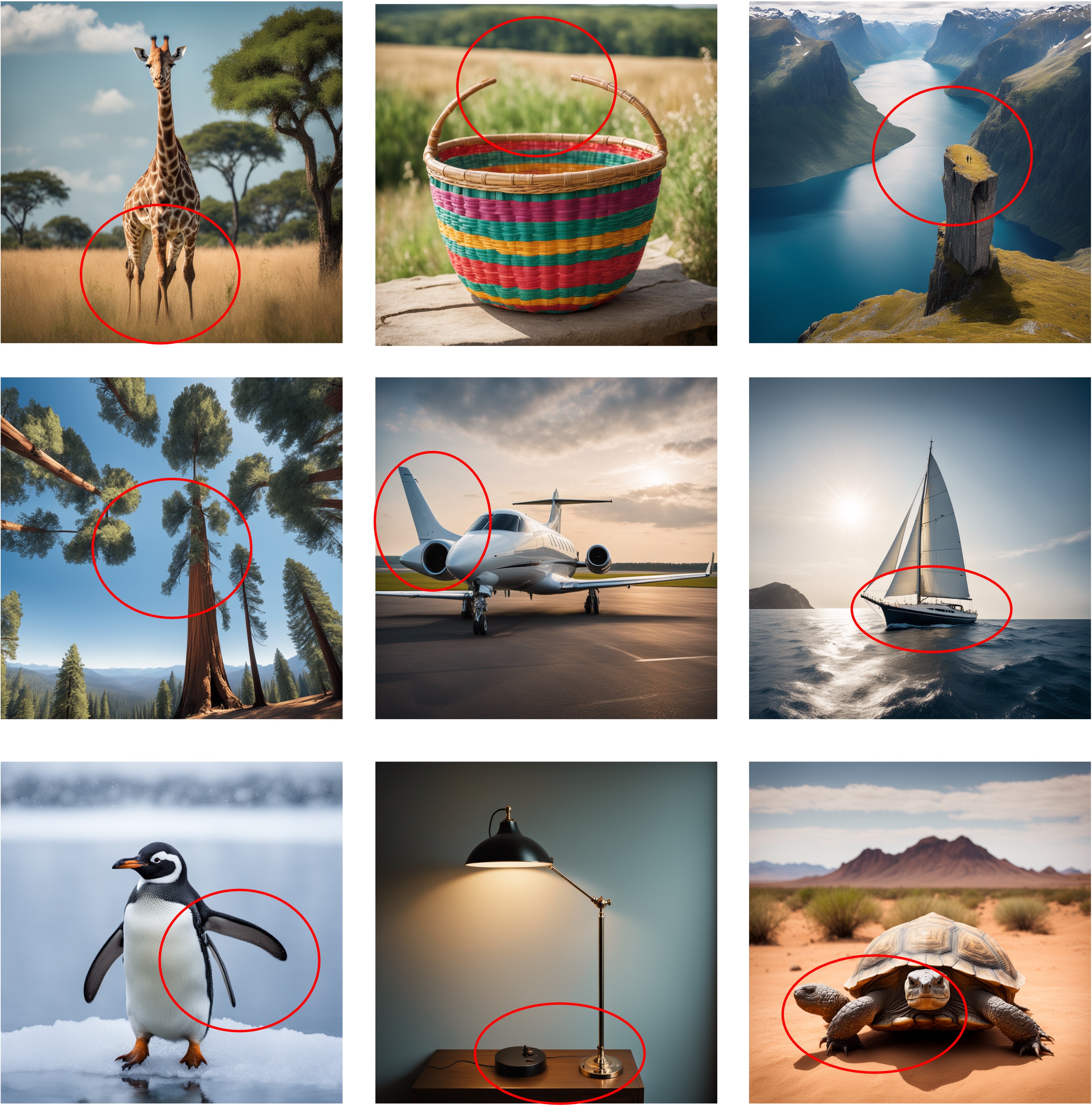
Figure 10: Some examples of excluded exemplars, highlighting the artifacts. A common artifact when generating animals was the wrong number of limbs (giraffe and penguin) or other body parts (the head of the tortoise). Other artifacts depicted here are layouts that did not follow the prompt (e.g., the sequoia), non-realistic perspectives (e.g., the horizon in sailboat), or compositions (e.g., the handle in basket, the reactor in jet plane, and the lamp stand in lamp (table)). Finally, despite the negative prompt, sometimes human figures made an appearance (e.g., in fjord pillar). Such images were also excluded.

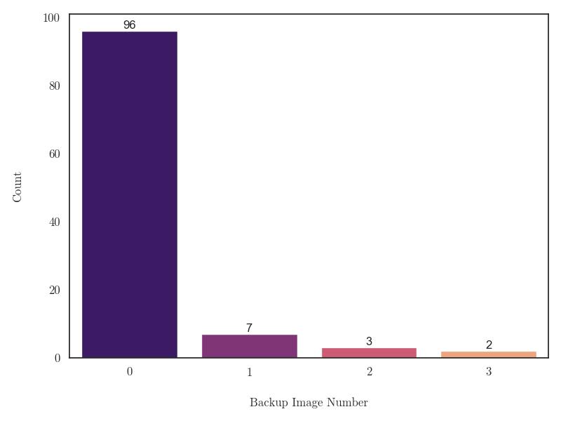
(a) Exclusion rates anchors

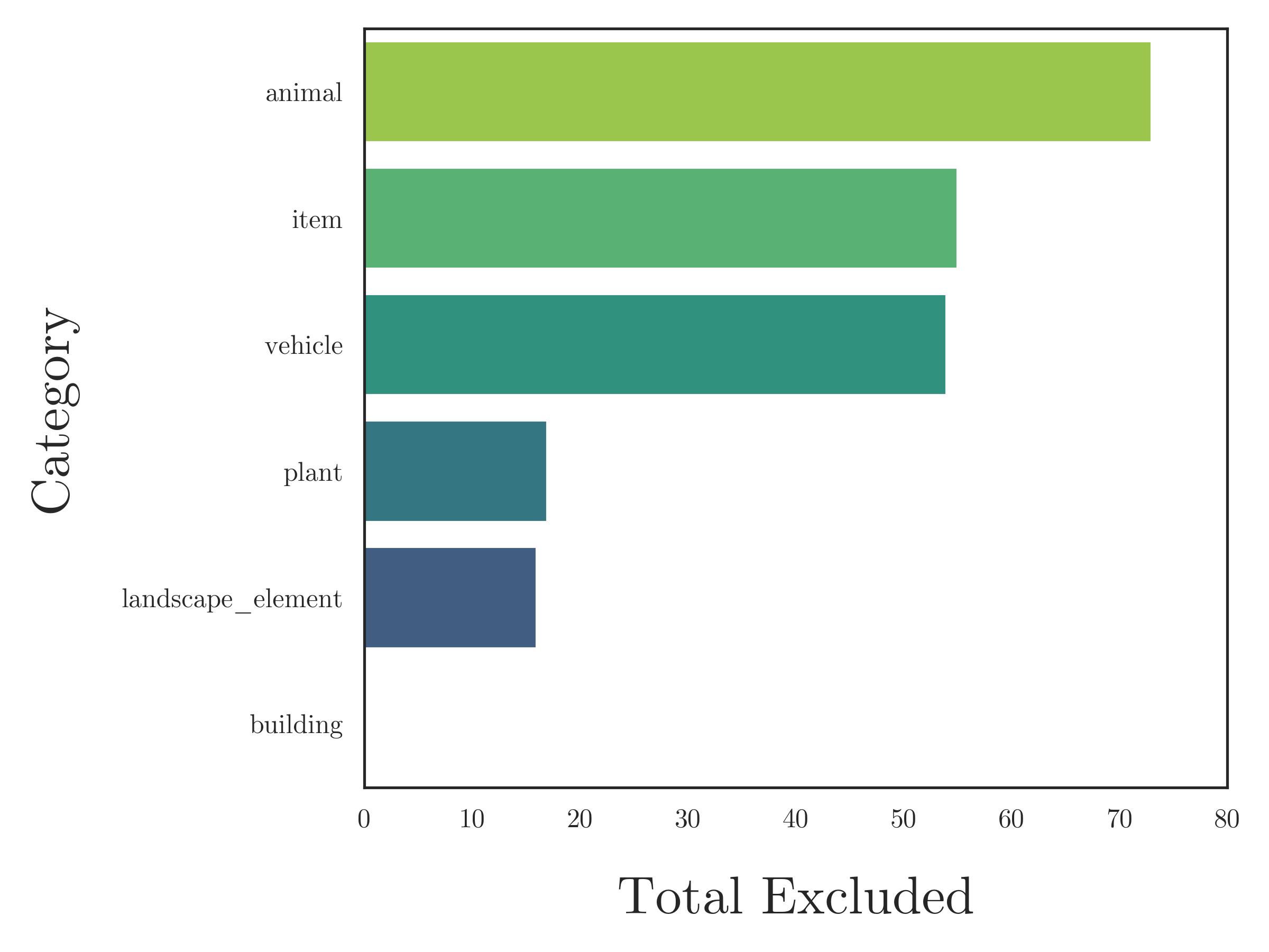
(b) Excluded by category

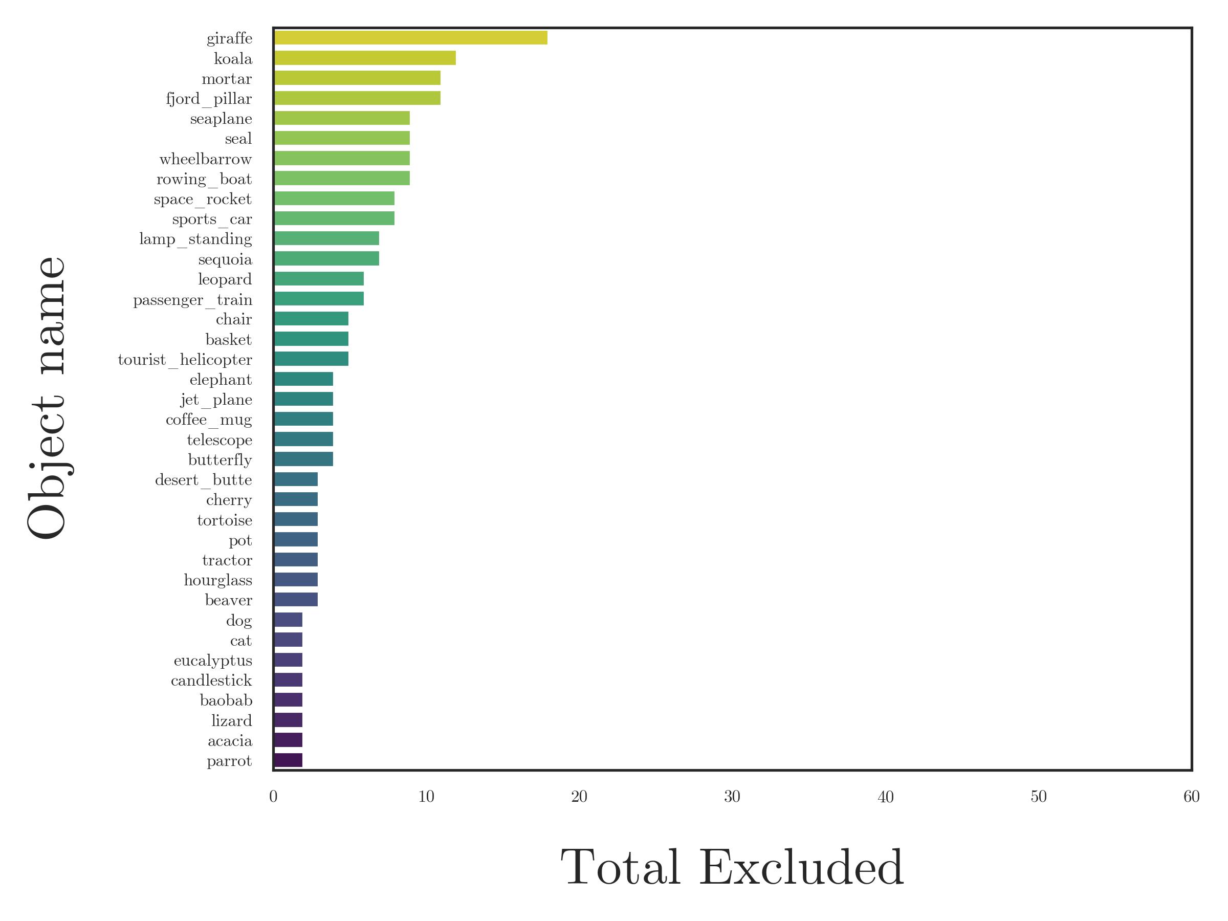
(c) Excluded by object

Figure 11: The giraffe had the highest number of exclusions, with 18 images excluded, which represents 30% of the 60 images for this object and 8.4% of the total 215 excluded images. This was followed by the koala with 12 exclusions (20% of its images and 5.6% of the total exclusions), and both the fjord pillar and mortar each with 11 exclusions (18.3% of their images and 5.1% of the total exclusions). The seal, seaplane, rowing boat, and wheelbarrow each had 9 exclusions (15% of their images and 4.2% of the total exclusions). The space rocket and sports car each had 8 exclusions (13.3% of their images and 3.7% of the total exclusions). Other notable exclusions included the lamp standing and leopard, each with 7 exclusions (11.7% of their images and 3.3% of the total exclusions), and the passenger train with 6 exclusions (10% of its images and 2.8% of the total exclusions). Objects such as the tourist helicopter, elephant, coffee mug, butterfly, and telescope had between 3 to 5 exclusions (ranging from 5% to 8.3% of their images and 1.4% to 2.3% of the total exclusions).

Table 3: Exclusion rates for all exemplar images.

	object	total_excluded	total_images	exclusion_rate
0	windmill	0	60	0.000000
1	polar_iceberg	0	60	0.000000
2	grassland_monolith	0	60	0.000000
3	greenhouse	0	60	0.000000
4	hill_river	0	60	0.000000
5	hot_air_balloon	0	60	0.000000
6	polar_base	0	60	0.000000
7	igloo	0	60	0.000000
8	pine_med	0	60	0.000000
9	kapok	0	60	0.000000
10	pine	0	60	0.000000
11	lake_island	0	60	0.000000
12	lamp_table	0	60	0.000000
13	lantern	0	60	0.000000
14	willow	0	60	0.000000
15	lighthouse	0	60	0.000000
16	lorry	0	60	0.000000
17	magnolia	0	60	0.000000
18	maple	0	60	0.000000
19	modern_building	0	60	0.000000
20	moorland_tor	0	60	0.000000
21	palm	0	60	0.000000
22	motorcycle	0	60	0.000000
23	mountain_glacier	0	60	0.000000
24	mountain_ridge	0	60	0.000000
25	mountain_rock	0	60	0.000000
26	oak	0	60	0.000000
27	observatory	0	60	0.000000
28	offroad_vehicle	0	60	0.000000
29	olive	0	60	0.000000
30	geothermal_spring	0	60	0.000000
31	fortress	0	60	0.000000
32	futuristic_building	0	60	0.000000
33	forest_boulder	0	60	0.000000
34	adobe_house	0	60	0.000000
35	bamboo_house	0	60	0.000000
36	wetland_tufa	0	60	0.000000
37	barn	0	60	0.000000
38	volcanic_peak	0	60	0.000000
39	vase	0	60	0.000000
40	bell_tower	0	60	0.000000
41	birch	0	60	0.000000
42	bottle	0	60	0.000000
43	bristlecone	0	60	0.000000
44	cabin	0	60	0.000000
45	car_vintage	0	60	0.000000
46	forest_river	0	60	0.000000
47	tea_house	0	60	0.000000
48	steam_locomotive	0	60	0.000000
49	teapot	0	60	0.000000
50	dragon_tree	0	60	0.000000
51	fishing_boat	0	60	0.000000
52	farm	0	60	0.000000
53	scooter	0	60	0.000000
54	sea_stack	0	60	0.000000
55	sofa	0	60	0.000000
56	pagoda	0	60	0.000000
57	skyscraper	0	60	0.000000
58	cactus	1	60	0.016667
59	shovel	1	60	0.016667
60	tropical_karst	1	60	0.016667
61	tropical_bird	1	60	0.016667
62	horse	1	60	0.016667
63	jar	1	60	0.016667
64	fish	1	60	0.016667
65	desert_arch	1	60	0.016667
66	sailboat	1	60	0.016667
67	owl	1	60	0.016667
68	frog	1	60	0.016667
69	campervan	1	60	0.016667
70	penguin	1	60	0.016667
71	parrot	2	60	0.033333
72	acacia	2	60	0.033333
73	lizard	2	60	0.033333
74	baobab	2	60	0.033333
75	candlestick	2	60	0.033333
76	eucalyptus	2	60	0.033333
77	cat	2	60	0.033333
78	dog	2	60	0.033333
79	beaver	3	60	0.050000
80	hourglass	3	60	0.050000
81	tractor	3	60	0.050000
82	pot	3	60	0.050000
83	tortoise	3	60	0.050000
84	cherry	3	60	0.050000
85	desert_butte	3	60	0.050000
86	butterfly	4	60	0.066667
87	telescope	4	60	0.066667
88	coffee_mug	4	60	0.066667
89	jet_plane	4	60	0.066667
90	elephant	4	60	0.066667
91	tourist_helicopter	5	60	0.083333
92	basket	5	60	0.083333
93	chair	5	60	0.083333
94	passenger_train	6	60	0.100000
95	leopard	6	60	0.100000
96	sequoia	7	60	0.116667
97	lamp_standing	7	60	0.116667
98	sports_car	8	60	0.133333
99	space_rocket	8	60	0.133333
100	rowing_boat	9	60	0.150000
101	wheelbarrow	9	60	0.150000
102	seal	9	60	0.150000
103	seaplane	9	60	0.150000
104	fjord_pillar	11	60	0.183333
105	mortar	11	60	0.183333
106	koala	12	60	0.200000
107	giraffe	18	60	0.300000

B.1.2 Pair selection using the LPIPS metric

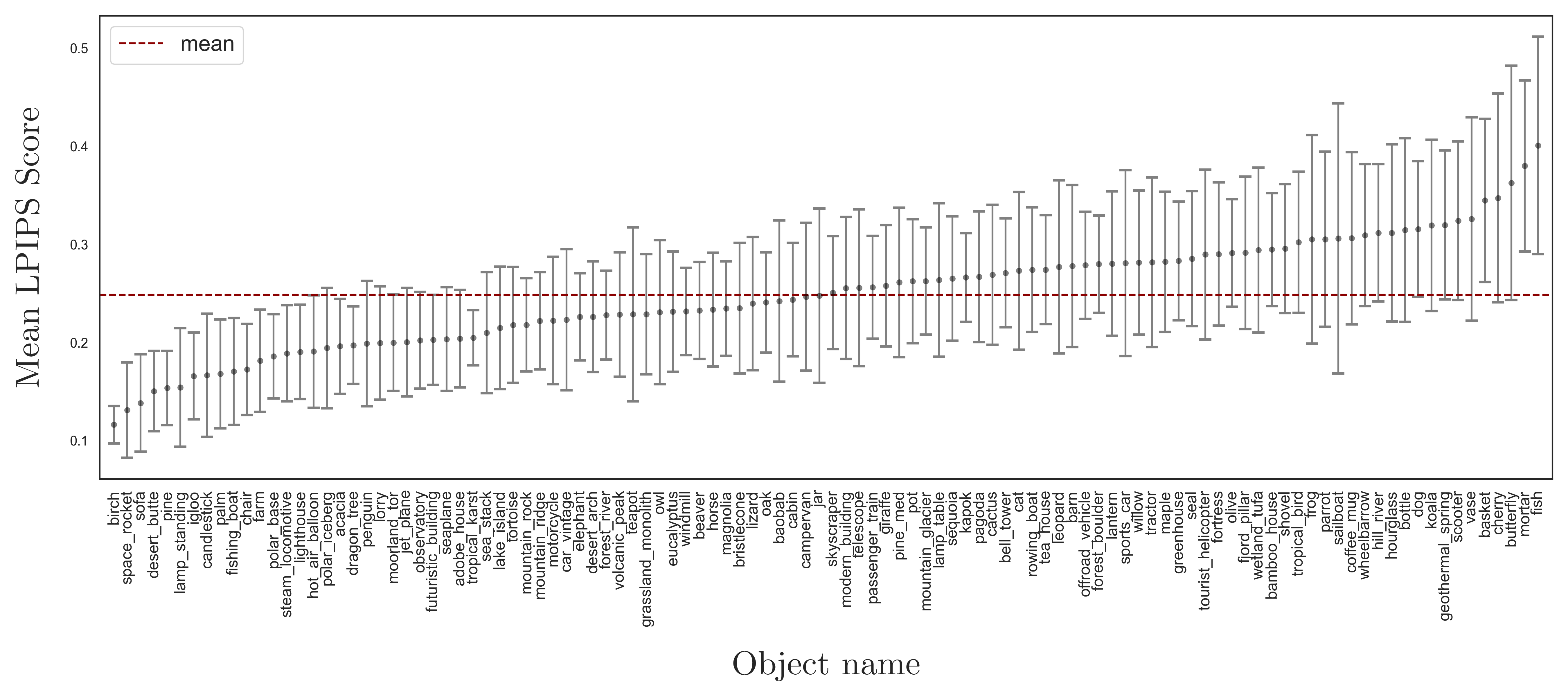
(b)

Figure 12: Mean LPIPS scores between exemplar images, grouped by a) category and b) object.

For each object, we calculated the LPIPS scores between all pairs of the exemplar images that had not been excluded (Figure 12). Overall, the mean LPIPS score across all objects was $0.453$ ($SD=0.054$). The object with the highest mean LPIPS score was fish ($M=0.589$, $SD=0.039$) and the one with the lowest was birch ($M=0.286$, $SD=0.344$). We then examined the distribution of mean LPIPS scores for each category. The category items had the highest mean LPIPS score ($M=0.483$, $SD=0.055$), followed by animal ($M=0.469$, $SD=0.068$), vehicle ($M=0.450$, $SD=0.028$), landscape element ($M=0.446$, $SD=0.054$), plant ($M=0.442$, $SD=0.055$), and building had the lowest mean score ($M=0.430$, $SD=0.043$). A one-way Analysis of Variance (ANOVA) revealed a statistically significant difference in mean LPIPS scores by category ($F(5,24)=2.54$, $p=0.033$). To investigate the pairwise differences more in detail, we conducted a post-hoc Tukey HSD test [84], which indicated a significant difference in mean LPIPS scores between the categories building and item (mean difference $=0.0538$, $p=0.030$). No other pairwise comparisons showed statistically significant differences in mean LPIPS scores ($p>0.05$). All test results are reported in Table 4.

group1	group2	meandiff	p-adj	lower	upper	reject
animal	building	-0.0399	0.2052	-0.0904	0.0106	False
animal	item	0.0139	0.9671	-0.0366	0.0644	False
animal	landscape_element	-0.0238	0.7459	-0.0743	0.0267	False
animal	plant	-0.0274	0.6156	-0.0779	0.0231	False
animal	vehicle	-0.0192	0.8779	-0.0697	0.0313	False
building	item	0.0538	0.0297	0.0033	0.1043	True
building	landscape_element	0.0161	0.9383	-0.0344	0.0666	False
building	plant	0.0125	0.9792	-0.038	0.063	False
building	vehicle	0.0207	0.8406	-0.0298	0.0712	False
item	landscape_element	-0.0377	0.2624	-0.0882	0.0128	False
item	plant	-0.0413	0.1747	-0.0918	0.0092	False
item	vehicle	-0.0331	0.4052	-0.0836	0.0174	False
landscape_element	plant	-0.0036	0.9999	-0.0541	0.0469	False
landscape_element	vehicle	0.0046	0.9998	-0.0459	0.055	False
plant	vehicle	0.0082	0.997	-0.0423	0.0587	False

Table 4: Multiple Comparison of Means - Tukey HSD, Family-Wise Error Rate (FWER) = 0.05, between LPIPS scores from all non-excluded anchor images. The table reports pairwise comparisons among different categories with the mean difference, adjusted p-values, and confidence intervals. Significant differences at the 0.05 level are indicated in the reject column.

Following the procedure illustrated in the Methods, for each object we selected a pair of images (an anchor image and a guide image) to interpolate. The performance of this procedure was assessed through visual inspection. In the vast majority of cases ($89.81\%$ of image pairs), our procedure successfully selected a suitable pair of images on the first attempt. However, in 11 cases ($10.18\%$), the initially selected second image did not meet our specified conditions (as detailed in the Methods section), necessitating the use of backup images. Specifically, we resorted to the second choice for 7 object pairs, the third choice for 3 pairs, and the fourth choice for 2 pairs. We assessed the statistical distribution of LPIPS scores between the selected pairs, that is the score between the anchor and the guide image (Figure 13). The mean LPIPS score was $0.35$ ($SD=0.067$). Pairs from the animal category had a mean score of $0.393$ ($SD=0.073$), from buildings had a mean score of $0.334$ ($SD=0.052$), from items had a mean score of $0.370$ ($SD=0.087$), from landscape elements had a mean score of $0.340$ ($SD=0.053$), from plants had a mean score of $0.335$ ($SD=0.063$), and from vehicles had a mean score of $0.339$ ($SD=0.052$). A one-way ANOVA test indicated a statistically significant difference in mean LPIPS scores across categories ($F(5,120)=2.525$, $p=0.034$). However, subsequent pairwise comparisons using the Tukey HSD test did not reveal significant differences between any specific pairs of categories (all $p>0.05$), see Table 5. This suggests that while pairs from different categories differed in mean LPIPS scores, these differences were relatively subtle.

group1	group2	meandiff	p-adj	lower	upper	reject
animal	building	-0.0589	0.0791	-0.1216	0.0039	False
animal	item	-0.0225	0.9033	-0.0852	0.0403	False
animal	landscape_element	-0.0533	0.1434	-0.1161	0.0094	False
animal	plant	-0.0577	0.0902	-0.1204	0.0051	False
animal	vehicle	-0.0541	0.1325	-0.1168	0.0086	False
building	item	0.0364	0.5448	-0.0263	0.0991	False
building	landscape_element	0.0055	0.9998	-0.0572	0.0683	False
building	plant	0.0012	1.0	-0.0616	0.0639	False
building	vehicle	0.0048	0.9999	-0.0580	0.0675	False
item	landscape_element	-0.0309	0.7096	-0.0936	0.0319	False
item	plant	-0.0352	0.5803	-0.0980	0.0275	False
item	vehicle	-0.0316	0.6873	-0.0944	0.0311	False
landscape_element	plant	-0.0044	1.0	-0.0671	0.0584	False
landscape_element	vehicle	-0.0008	1.0	-0.0635	0.0620	False
plant	vehicle	0.0036	1.0	-0.0591	0.0663	False

Table 5: Multiple Comparison of Means - Tukey HSD, FWER=0.05, between LPIPS scores from selected pairs of anchor and guide images in the interpolations. The table presents mean differences, adjusted p-values, and confidence intervals for each pairwise comparison.

B.1.3 Interpolations

For each of the 108 object pairs, we generated 200 interpolated images (including the anchor and the guide images). Following the criteria explained in the Methods, we selected 10 images for each object, including the anchor image and 9 of its interpolations. To achieve this, we first computed the LPIPS score between the anchor image and each interpolated image (Figure 15).

Overall, the mean LPIPS score across all objects was $0.249$ ($SD=0.055$). The object with the highest mean LPIPS score was fish ($M=0.401$, $SD=0.111$), and the one with the lowest was birch ($M=0.116$, $SD=0.019$). The object with the highest standard deviation in LPIPS scores was sailboat in the vehicle category ($M=0.306$, $SD=0.138$), whereas the object with the lowest standard deviation in LPIPS scores was birch in the plant category ($M=0.116$, $SD=0.019$). We then examined the mean LPIPS scores for each category. Animal had a mean LPIPS score ($M=0.277$, $SD=0.053$), followed by item ($M=0.264$, $SD=0.069$), landscape element ($M=0.238$, $SD=0.045$), plant ($M=0.238$, $SD=0.055$), building ($M=0.237$, $SD=0.042$), and vehicle ($M=0.237$, $SD=0.053$). A one-way ANOVA revealed no statistically significant difference in mean LPIPS scores across categories ($F(5,24)=1.919$, $p=0.098$).

We defined target similarity scores that were linearly spaced between the minimum and maximum LPIPS values observed for each object. For each target score, we selected the image whose similarity score was closest to the target score, ensuring no duplicates. We visually inspected the interpolated images to exclude those with artefacts and maintain a high level of quality and consistency. Given the vast number of images (21,600 in total), the visual inspection was performed only after selecting the interpolated images of interest. For each object, we assessed how many interpolations needed to be swapped with one of their neighbours. The vast majority of objects ($87.62\%$) required no swaps, while a total of $16$ objects ($14.81\%$) required one or more swaps. Among those, $8$ were from animal ($44.4\%$ of the objects from that category), $4$ from item ($22.2\%$), $3$ from vehicle ($16.7\%$), and $1$ from landscape element ($5.5\%$). See Figure 14.

We performed a Pearson correlation to assess the relationship between exclusion rates in anchor images and swap rates in interpolated images. The analysis revealed a significant positive correlation ($r=0.531$, $p<0.001$), indicating that objects with higher exclusion rates in exemplar images also tended to have higher swap rates in interpolated images, suggesting consistent issues with the generation of certain objects (Figure 16). The most problematic was the animal category, with an average exclusion rate of $0.068$ and an average swap rate of $0.094$. The least problematic categories were building and plant, both with no exclusions. Additionally, the building category had no swaps, while the plant category had a minimal swap rate ($0.016$).

(a)

(a)

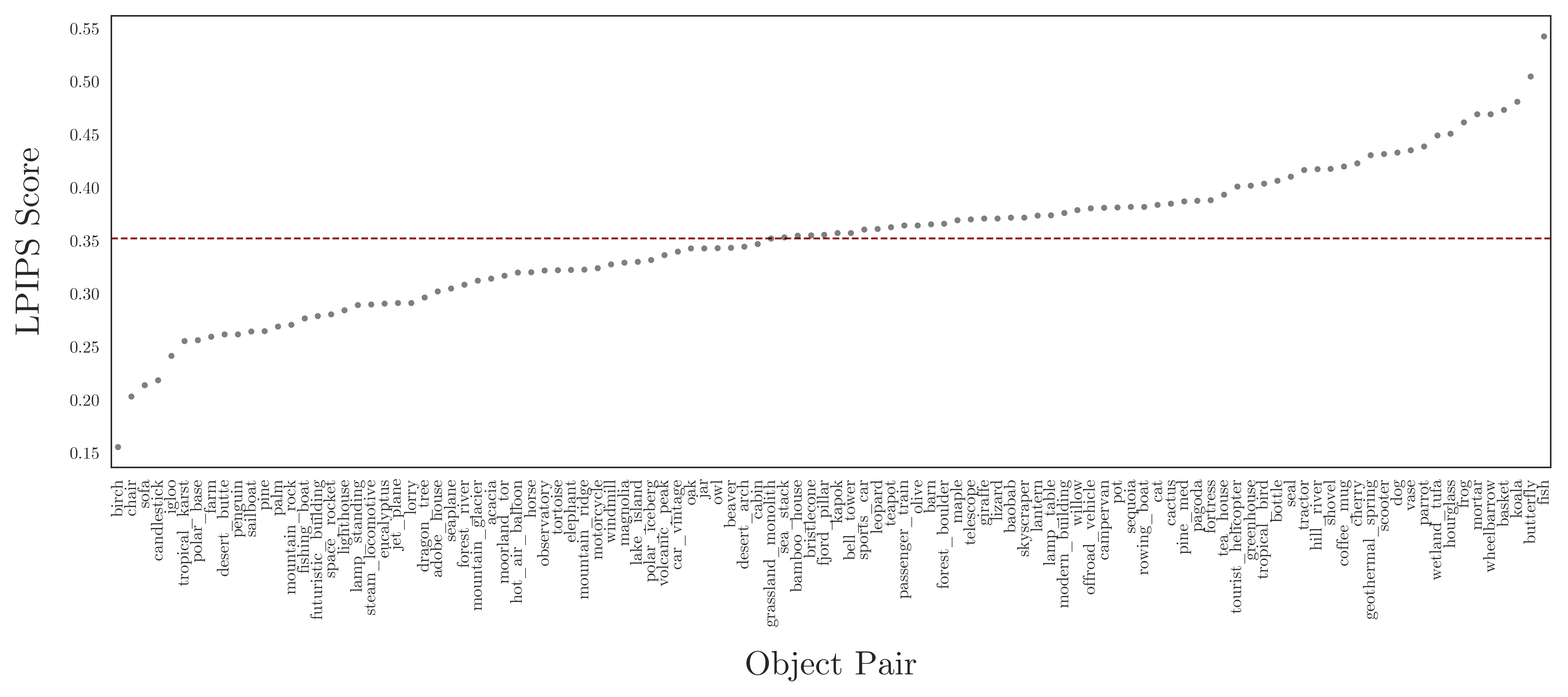
(b)

Figure 13: Mean LPIPS scores for selected pairs, grouped by object and category. a) Distribution of mean LPIPS scores by category. Each data point is the mean LPIPS score for an object belonging to that category (18 data points in total). The category means are shown in red. b) Mean LPIPS scores by object, ordered by magnitude. Lower scores indicate more homogeneity (i.e. highest similarity) between the exemplar images. The red dotted line is the overall mean across all similarity scores.

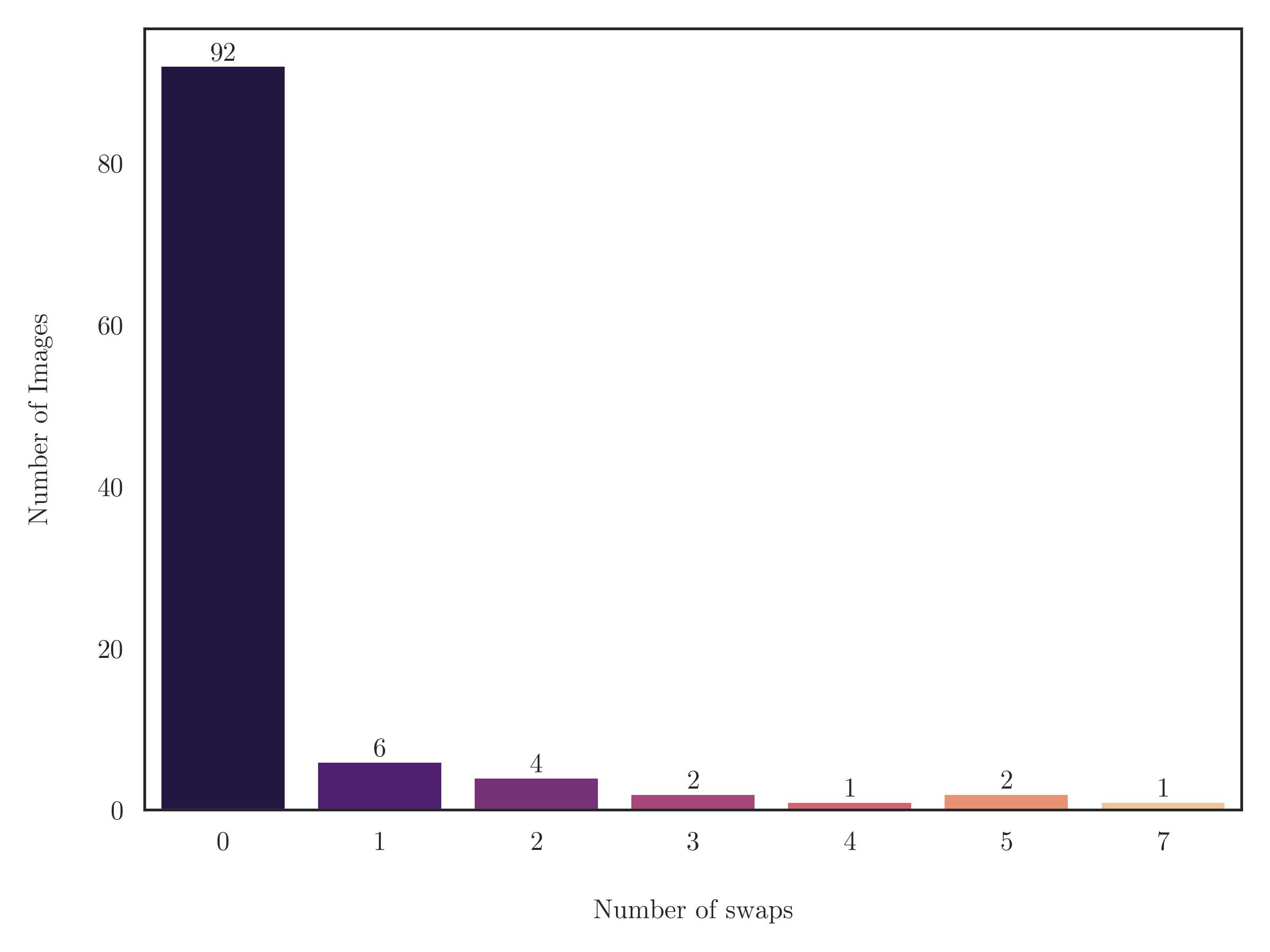
Figure 14: Swapped interpolations. Specifically, the following objects required swaps: butterfly, horse, koala, and owl each required $1$ swap ($10\%$). The mortar in the item category required $1$ swap ($10\%$), and the table lamp required $2$ swaps ($20\%$). The fjord pillar in landscape elements required $1$ swap ($10\%$). Among animals, the cat, leopard, and parrot each required $2$ swaps ($20\%$). For vehicles, the passenger train and seaplane required $3$ swaps each ($30\%$), and the rowing boat required $5$ swaps ($50\%$). The teapot required $4$ swaps ($40\%$), and the telescope required $5$ swaps ($50\%$) in the item category. The giraffe had the highest number of swaps, with $7$ swaps ($70\%$).

(a)

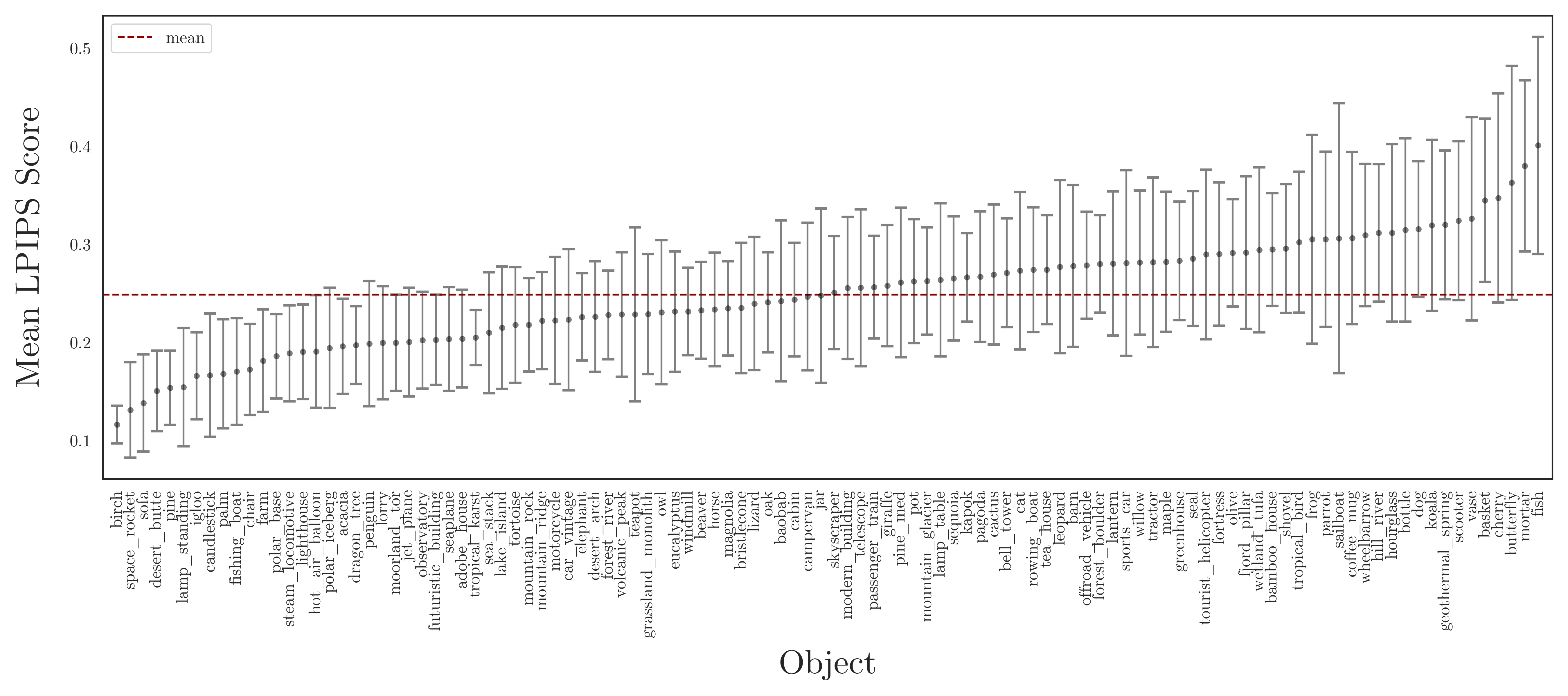
(b)

Figure 15: Mean LPIPS scores between anchor images and each interpolated image, grouped by a) category and b) single objects.

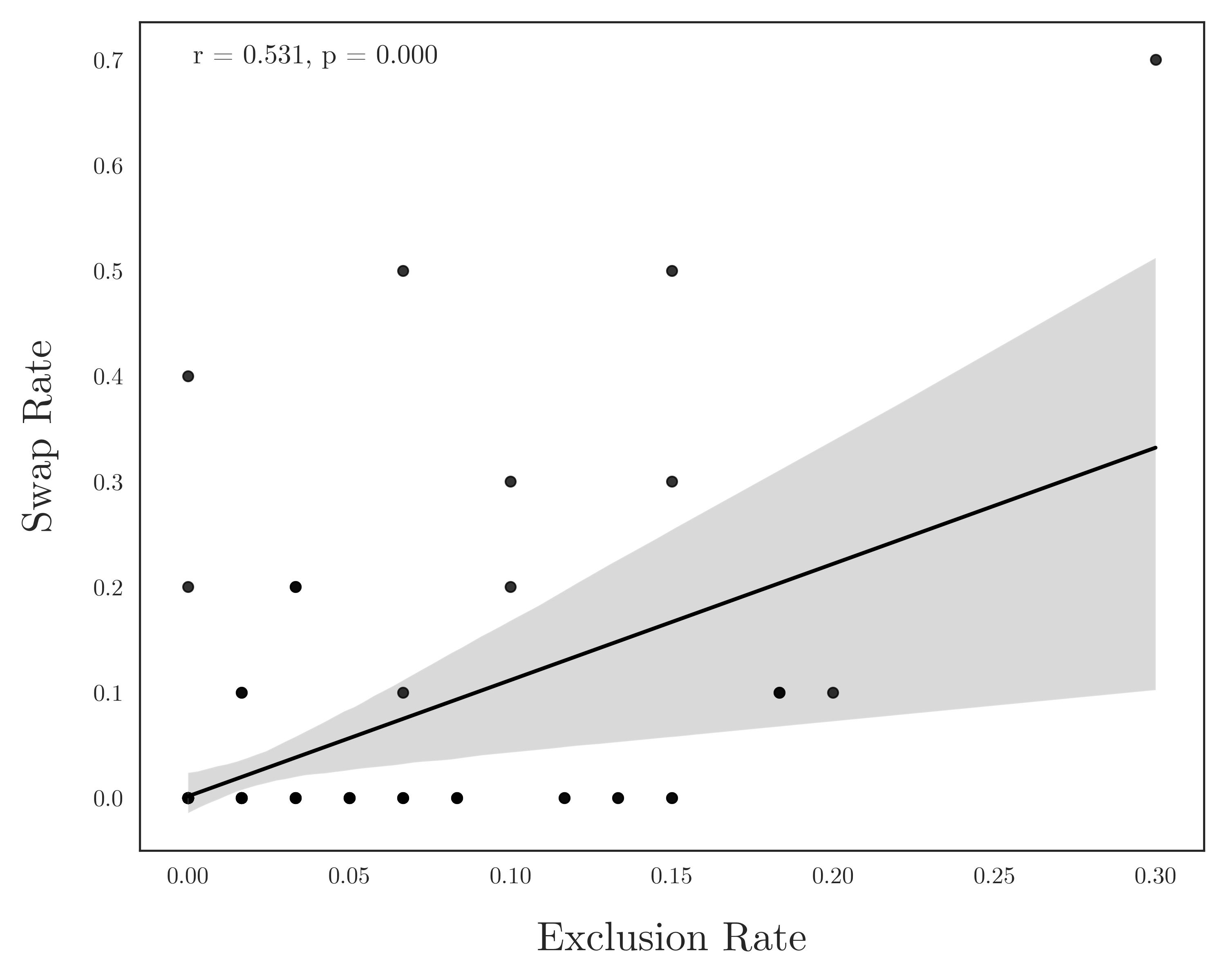
Figure 16: Correlation between exclusion and swap rates.

B.1.4 Physical characteristics of the stimulus set

Figure 17(b) shows the feature distributions by category. Contrast varies, with animal and building showing higher levels and symmetrical distributions. Mean pixel intensity is higher in building and item, with normal distributions. Relative luminance is uniform across categories, with animal slightly higher and a symmetrical distribution. Colourfulness is higher in plant and landscape element, with normal distributions. Entropy is consistent across categories, with item and vehicle showing higher values and slightly left-skewed distributions. Edge density is higher in animal and item, with right-skewed distributions. Blur is higher in building and item, with symmetrical distributions. Sharpness is higher in animal and item, with right-skewed distributions. Image energy is higher in building and item, with right-skewed distributions. High spatial frequency is higher in building and item, with slightly left-skewed distributions.

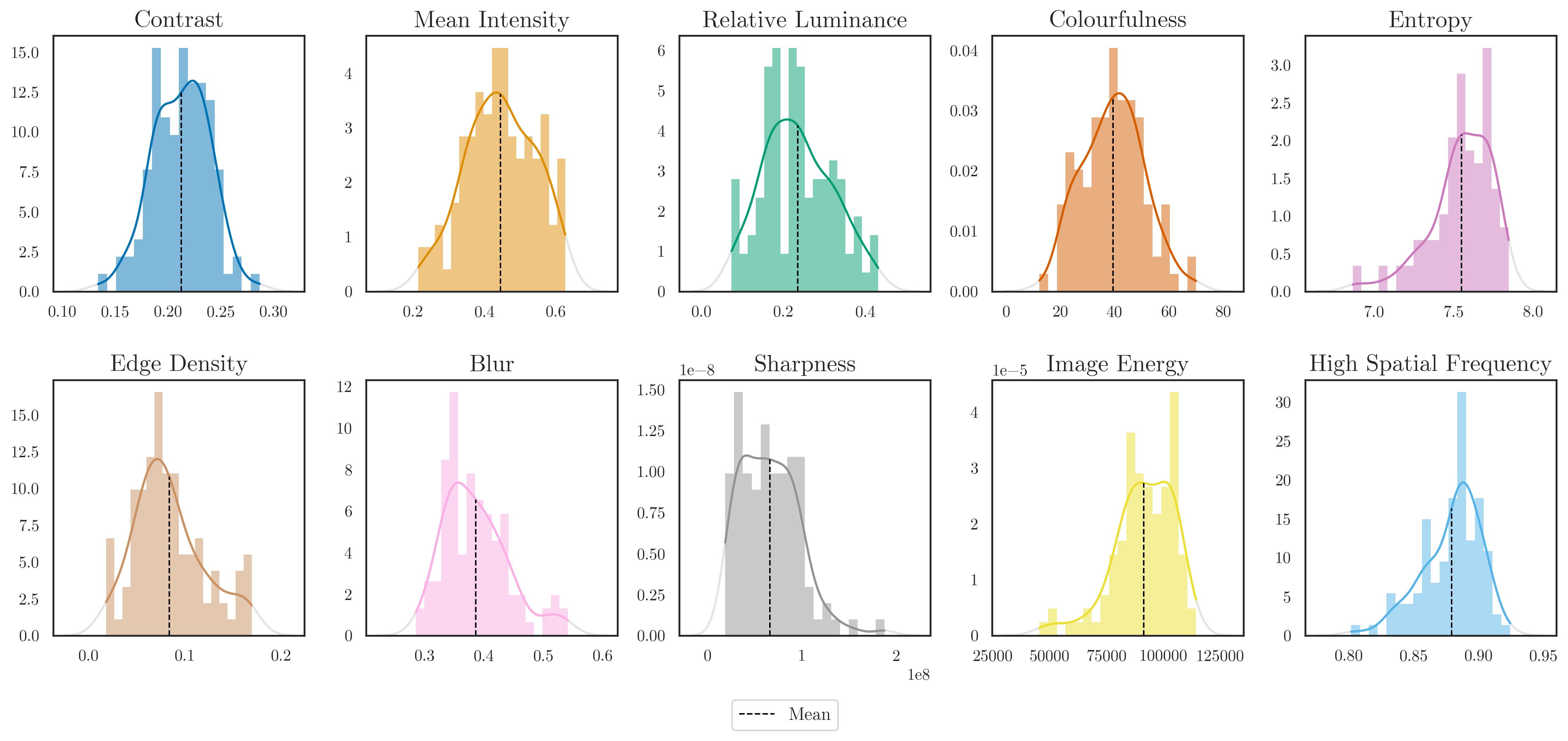
(a)

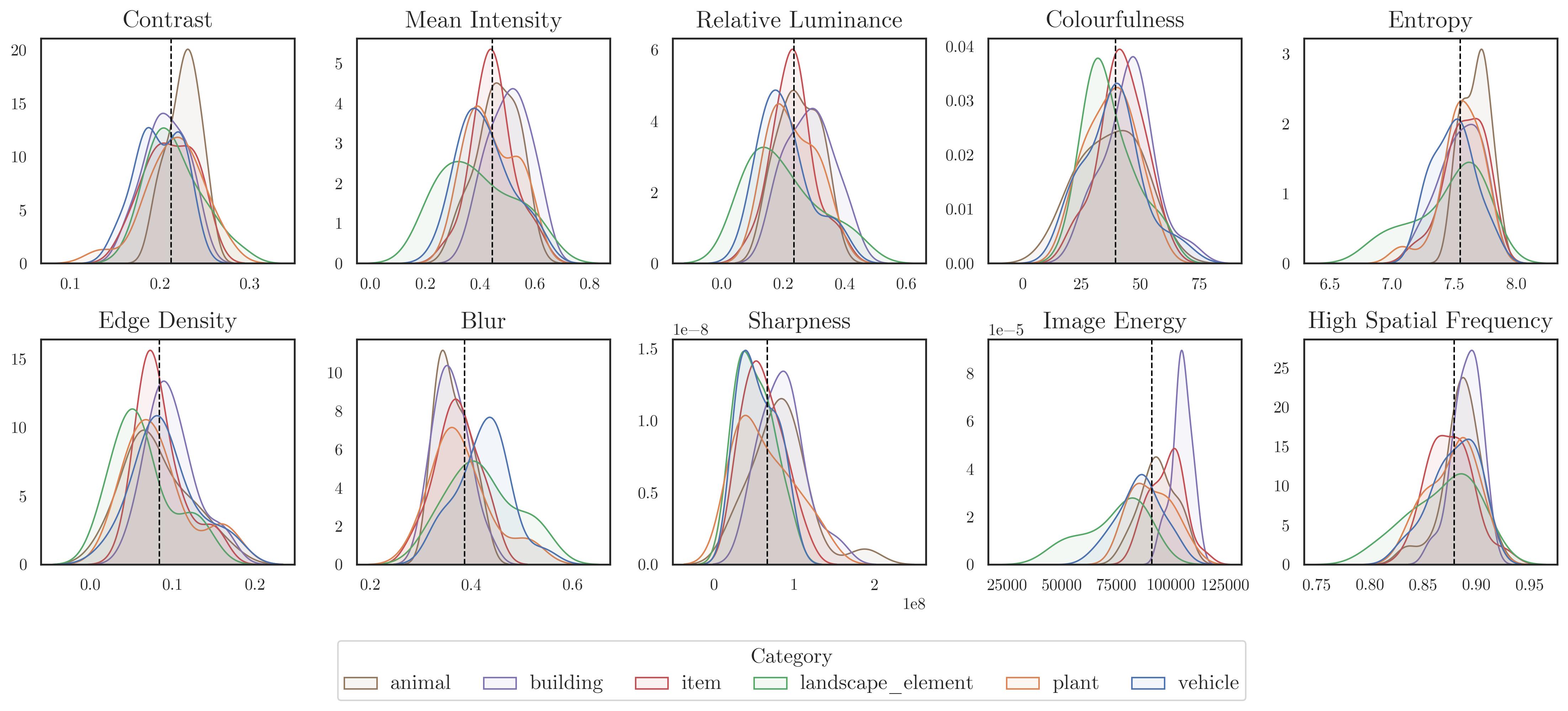
(b)

Figure 17: Physical characteristics of the anchor images of the final stimulus set. a) The first set of histograms illustrates the overall distributions of various image features across the stimulus set. Each feature is accompanied by a fitted density curve and a dashed line indicating the mean value. b) The second set of plots provides a comparison of feature distributions across different image categories (animal, building, item, landscape element, plant, vehicle). Each plot shows the distribution of a feature for each category, with the overall mean indicated by a dashed line.

B.2 Similarity judgement task

B.2.1 Online task

The median experiment duration was $24.11$ minutes and the median duration of the triplet comparison task (excluding instructions and training) was $20.5$ minutes. The median reaction time in the task was $1501.0$ ms (Figure 18(a)).

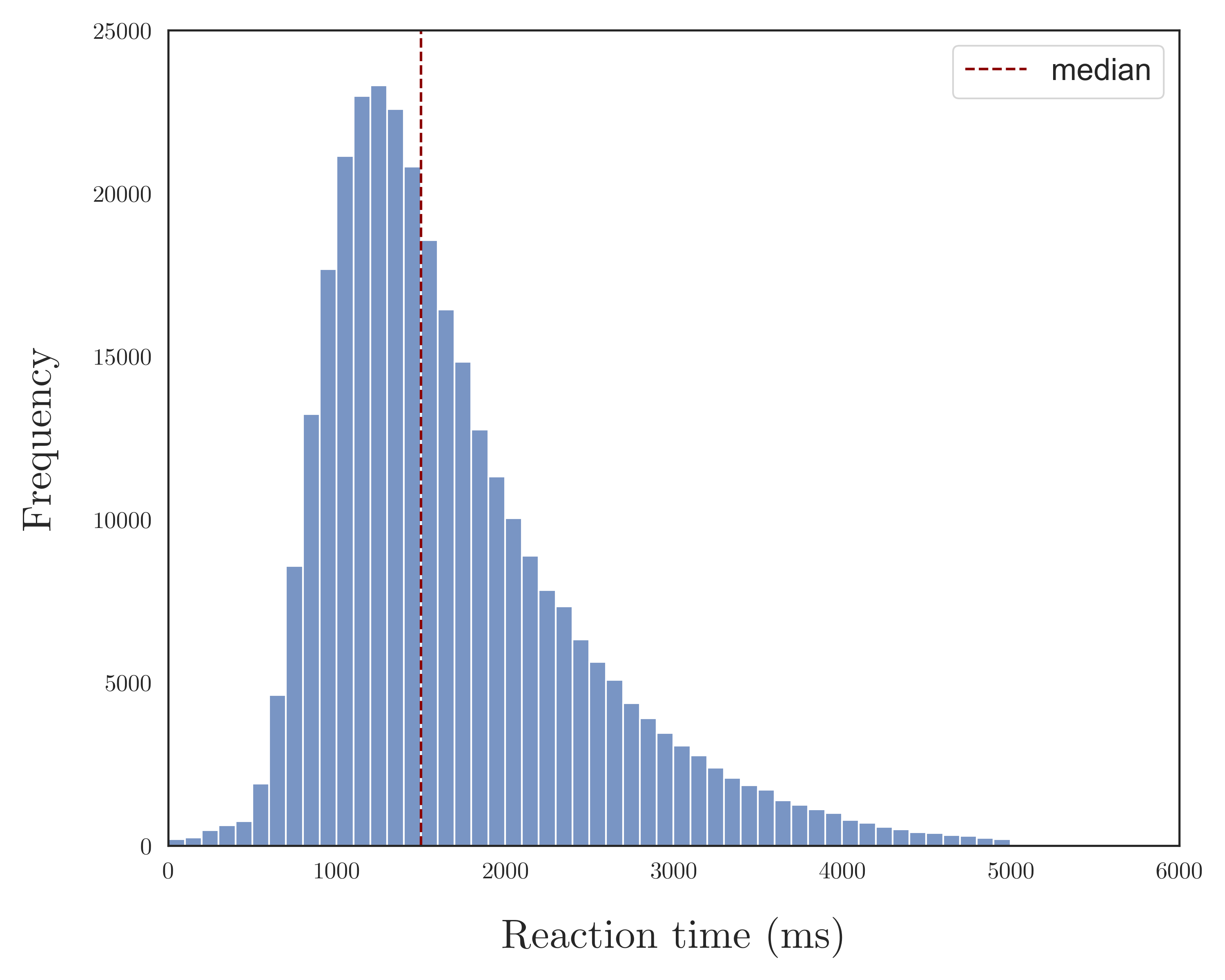
(a)

(b)

(c)

Figure 18: Distributions aggregated over all participants’ data: (a) Reaction time distribution, (b) Reaction time distributions for each category, and (c) Reaction time distributions for all participants in the final sample ($RT<6000\,\text{ms}$), sorted by participant ID in descending order of mean reaction time.

B.2.2 Evaluation of the embeddings

The performance of the three embedding algorithms of interest — t-STE, SOE, and MLDS — was evaluated using the Leave-One-Participant-Out cross-validated triplet error. In order to assess the overall performance of each model, we calculated the mean cross-validated error by method, averaging across all objects. The mean cross-validated triplet error rates were 0.313 for MLDS, 0.280 for t-STE, and 0.279 for SOE (Figure 19(a)). A one-way ANOVA revealed a significant effect of the embedding algorithm on the triplet error rate, $F(2,87)=114.3,p<0.0001$. Post-hoc comparisons using the Tukey HSD test indicated that both t-STE and SOE had significantly lower triplet error rates compared to MLDS ($p<0.05$). Specifically, the mean difference between MLDS and SOE was -0.0335 ($95\%\,\text{CI}=[-0.0395,-0.0276]$), and between MLDS and t-STE was -0.0332 ($95\%\,\text{CI}=[-0.0391,-0.0272]$), both significant at $p<0.05$. There was no significant difference between t-STE and SOE (mean difference = 0.0004, $95\%\,\text{CI}=[-0.0056,0.0064]$, $p=0.9872$).

We also assessed object-specific and category-specific performance by aggregating and averaging the cross-validated errors for each object (Figure 19(d)) and category (Figure 19(c)). Our analysis revealed that t-STE and SOE consistently performed well across different objects. In contrast, MLDS showed significant performance variability, with a notable error increase for certain objects. For instance, the triplet error for “moorland tor” was 0.48 with MLDS, compared to 0.304 for SOE and 0.305 for t-STE. The analysis of category-specific performance showed that t-STE and SOE consistently outperformed MLDS across all categories. Notably, t-STE and SOE had very similar performance, with negligible differences in triplet errors.

B.2.3 Stability of the embedding values

The cross-validated triplet error provides a performance estimate for each algorithm, indicating how well the estimated embeddings generalise to unseen triplets across participants. Since we were ultimately interested in using the participants’ judgements to order the images along a perceptual scale determined by the embedding values, we assessed their stability. Embedding estimates are only useful to this purpose if they are reasonably coherent across the sample and not overly sensitive to variations in the source data. We analysed the influence of data from individual participants on the final embedding values by comparing the object-specific embedding estimates across different folds for each algorithm. In general, we found that SOE provided more stable embedding estimates, making it more robust to variations in the source data. A few object-specific examples are provided in Figure 20.

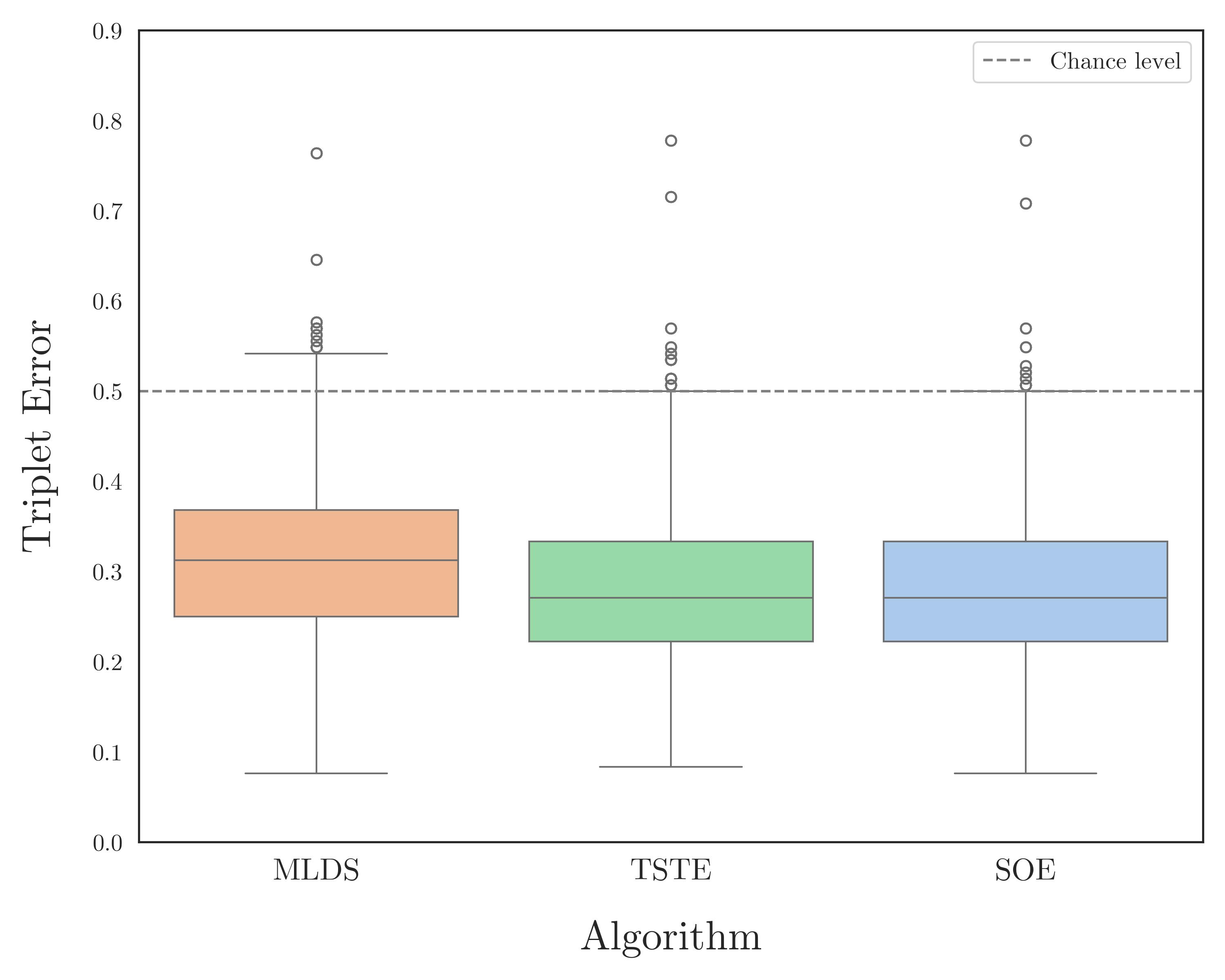
(a)

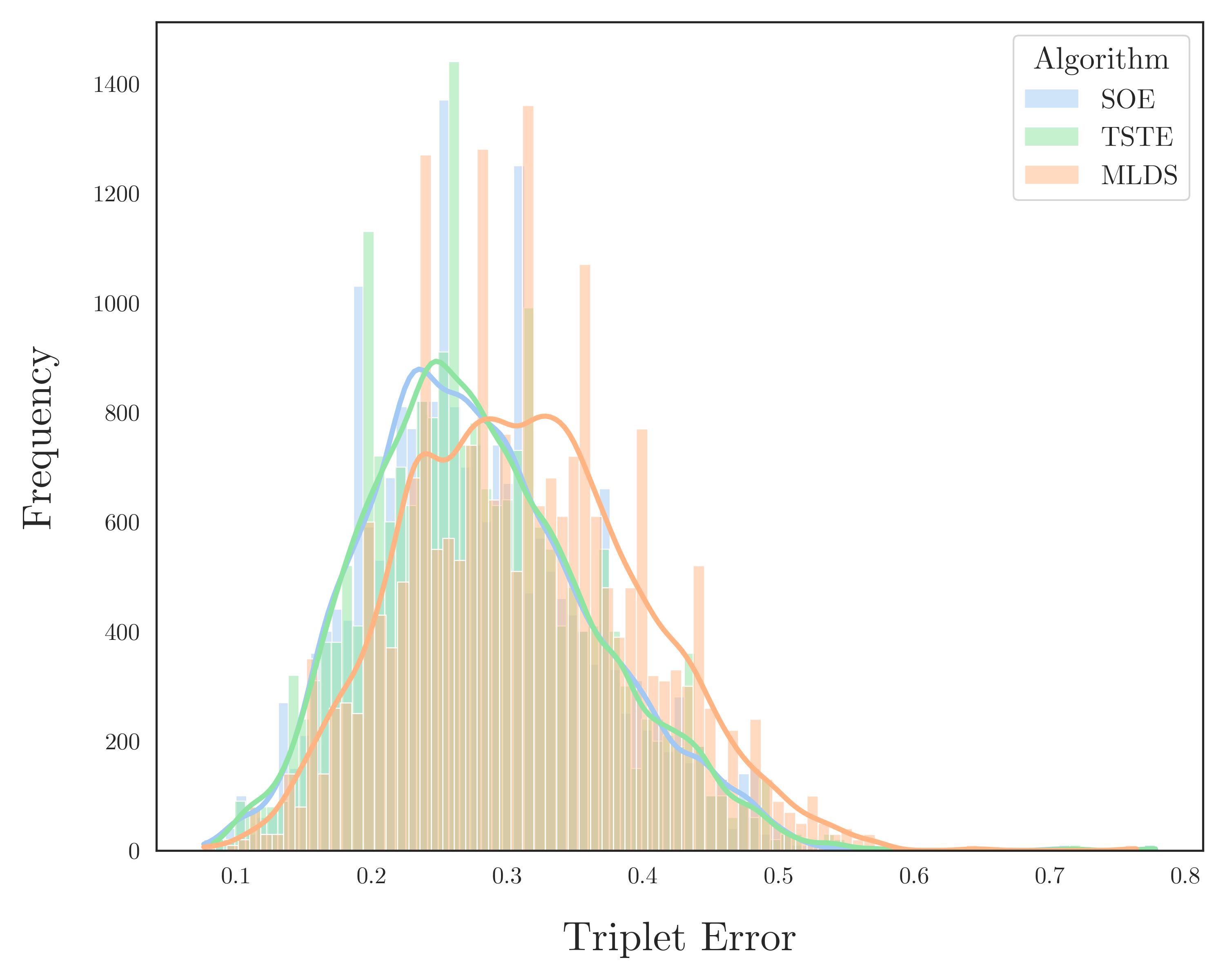
(b)

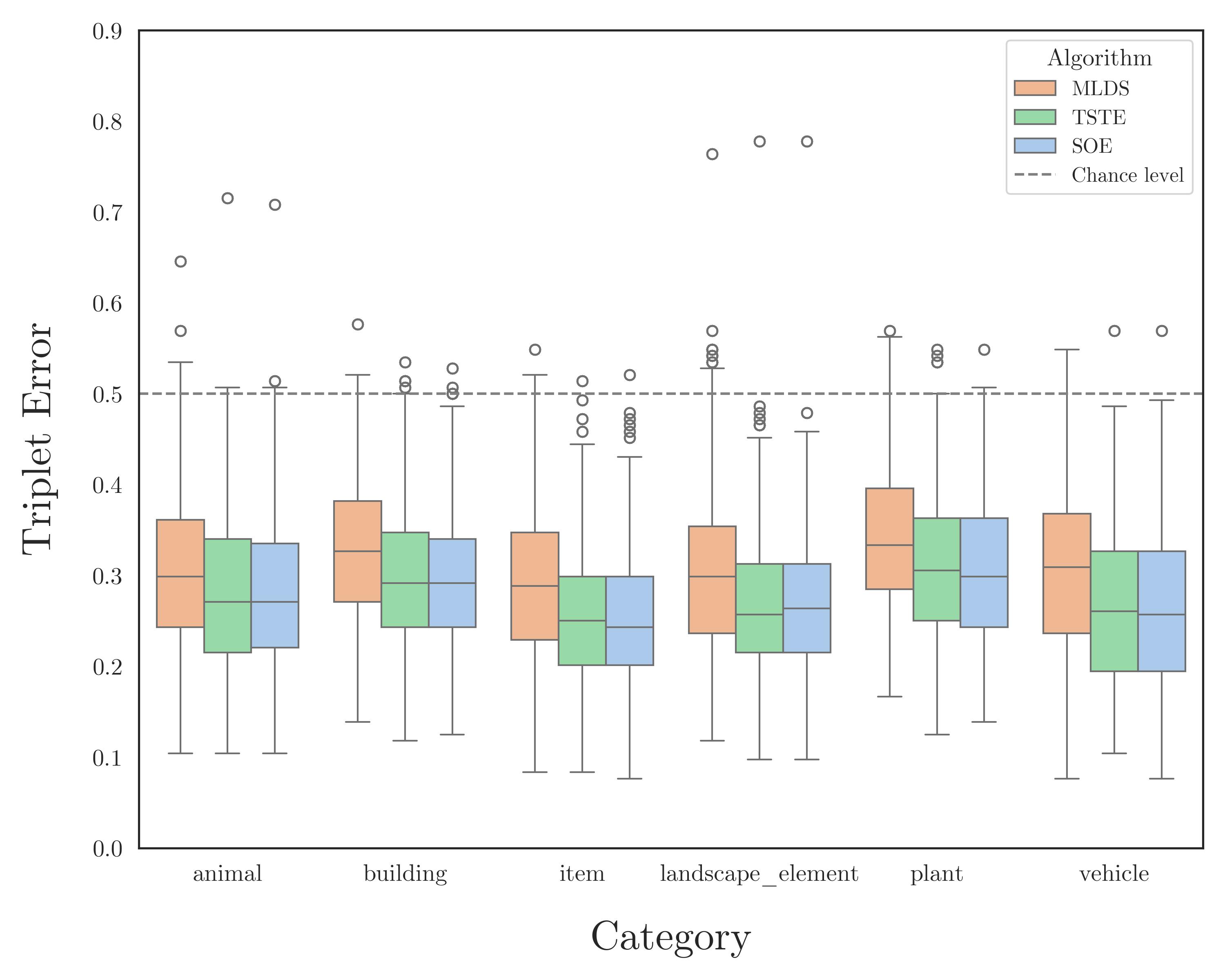
(c)

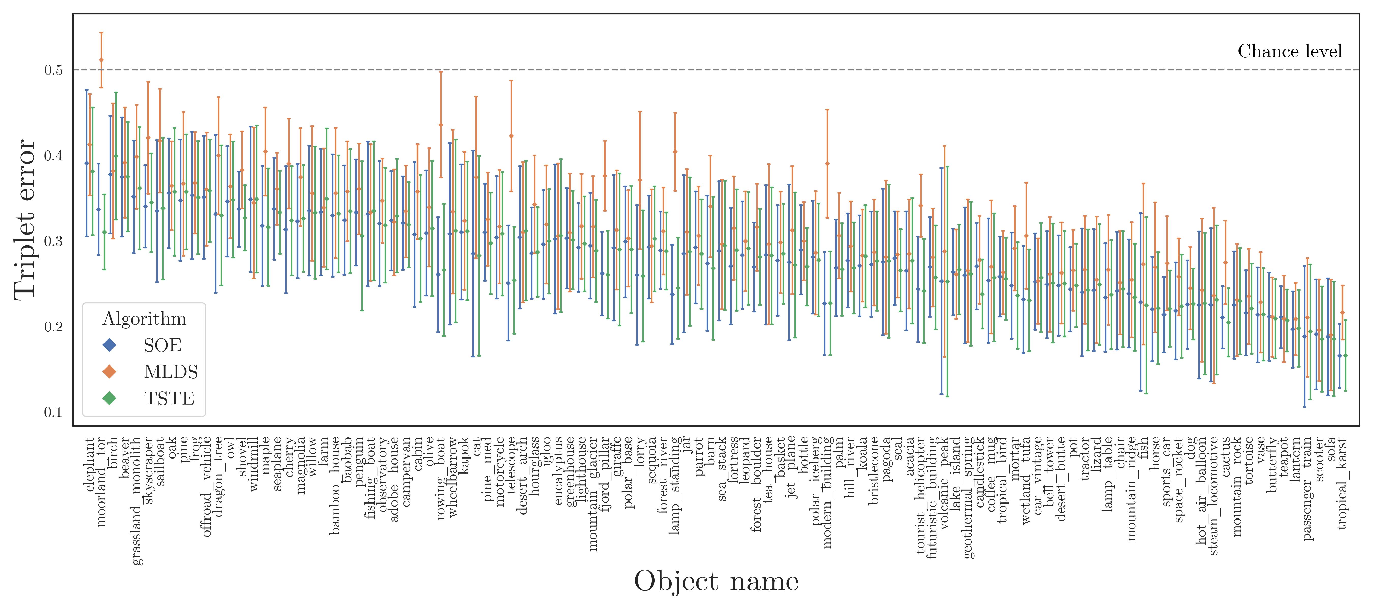
(d)

Figure 19: Comparative performance analysis of SOE, t-STE, and MLDS algorithms using triplet error. (a) Overall performance: mean triplet error across conditions. (b) Error distributions: variability per algorithm as histograms. (c) Category-specific performance: triplet error across object categories. (d) Object-specific performance: triplet error for individual objects.

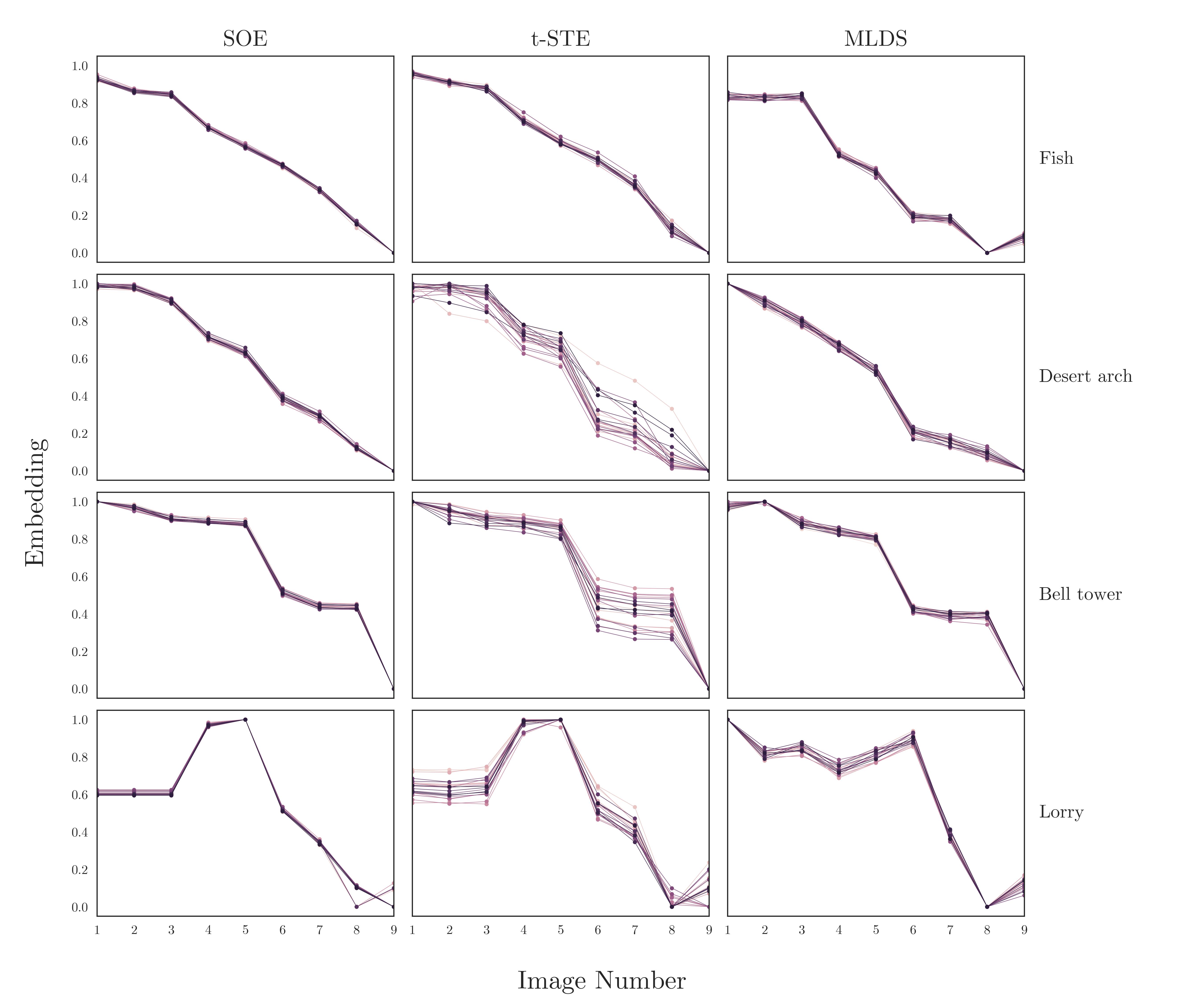
Figure 20: Visualisation of the variability of embedding estimates across algorithms for a) desert arch, b) fish, c) bell tower, d) lorry. Each line represents embedding values estimated from one cross-validation fold, where one participant is left out. This illustrates the sensitivity of the estimates to individual participants. SOE yields more robust estimates compared to the other algorithms, though all perform well overall. The image order on the x-axis follows the model-based similarity metric (LPIPS), not the participants’ reordered judgments. This explains why the lines are not monotonic, as the model ranking does not necessarily correspond to the participants’ evaluations.

B.3 Reordering the image variations

Although we found no significant difference in performance between SOE and t-STE in terms of triplet error, SOE showed more consistent embedding values across iterations, reducing variability in the results (Figure 20). Therefore, we decided to use the embedding values estimated by SOE to order the image variations on a perceptual scale for each object. The values were computed object-wise, using the aggregate data from all participants. In total, 95 objects (88%) saw at least one position reordering, whereas 13 objects maintained the order provided by the LPIPS score (Figure 21). The median number of reorderings per object was 3. To quantify the degree of agreement between the ordinal positions derived from LPIPS scores and those from SOE embeddings, we calculated a Spearman’s rank correlation. The analysis revealed a positive correlation, $\rho(1078)=0.73$, $p<0.001$, indicating that the ordinal positions based on the LPIPS metric align with those based on the SOE embedding values. We provide some examples of the stimulus set after psychophysical validation in Figure 4. For a comparison between the LPIPS-based order and the order after the behavioural task.

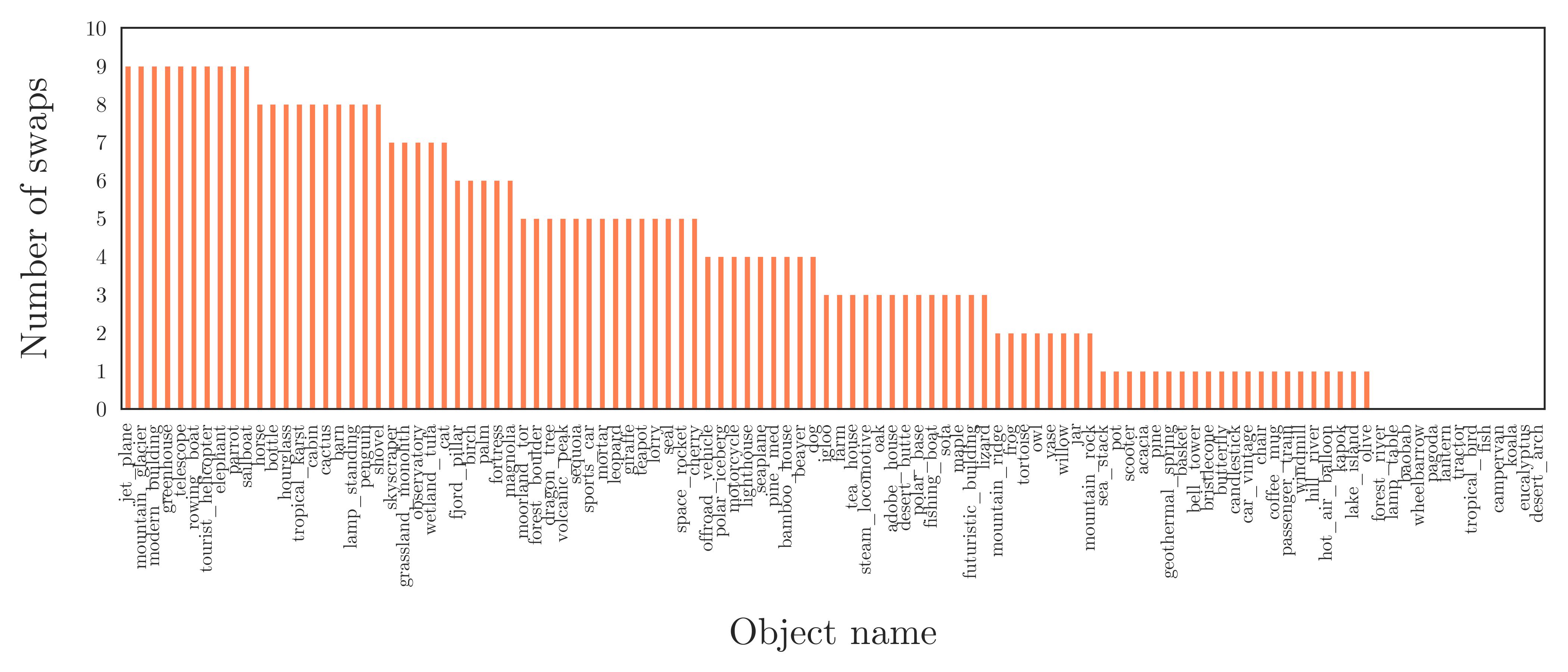
Figure 21: Reordering count by object.

B.4 Embedding analyses

MLDS, T-STE and SOE generally produced comparable results. This corroborates other studies relying on simulations that showed a substantial equivalence in performance for low-dimensional cases [85]. One open issue is to what extent the embedding values reflect real differences in perceptual similarity.

One limitation of using the embedding values to reorder the images on a perceptual scale is that it is not very robust to small variations in embedding due to noise. This is due to the fact that some of the image variations are very similar to one another and have very similar embedding values. In these cases, the ordinal position of the stimuli is susceptible to noise fluctuations. At the same time, it should be noted that not all reorderings are perceptually meaningful. When stimuli have similar embedding values, it means that participants did not perceive significant differences between them. They can therefore be considered a “perceptual cluster”, within which the order of the stimuli is relatively stochastic.

We made the simplifying assumption that each set of image variations can be ranked using a single dimension that follows the LPIPS metric. An open question is what stimulus features within the objects drove the similarity judgements more strongly and future work should address that. However, we found that – in most cases – it was possible to order naturalistic stimuli along one perceptual dimension in good agreement with the LPIPS metric. Our results extend the existing literature showing that the triplet comparison method can be effectively used for naturalistic images, even for perceptually subtle variations.

References

- [1] J. M. Henderson and A. Hollingworth, “High-level scene perception,” Annual review of psychology, vol. 50, no. 1, pp. 243–271, 1999.
- [2] M. Bar, “Visual objects in context,” Nature Reviews Neuroscience, vol. 5, no. 8, pp. 617–629, 2004.
- [3] A. Oliva and A. Torralba, “The role of context in object recognition,” Trends in Cognitive Sciences, vol. 11, p. 520–527, Dec. 2007.
- [4] R. A. Epstein and C. I. Baker, “Scene perception in the human brain,” Annual Review of Vision Science, vol. 5, p. 373–397, Sept. 2019.
- [5] L. Goetschalckx, A. Andonian, and J. Wagemans, “Generative adversarial networks unlock new methods for cognitive science,” Trends in Cognitive Sciences, vol. 25, pp. 788–801, Sept. 2021.
- [6] J. G. Snodgrass and M. Vanderwart, “A standardized set of 260 pictures: Norms for name agreement, image agreement, familiarity, and visual complexity.,” Journal of Experimental Psychology: Human Learning and Memory, vol. 6, no. 2, p. 174–215, 1980.
- [7] M. B. Brodeur, E. Dionne-Dostie, T. Montreuil, and M. Lepage, “The bank of standardized stimuli (boss), a new set of 480 normative photos of objects to be used as visual stimuli in cognitive research,” PLoS ONE, vol. 5, p. e10773, May 2010.
- [8] J. Deng, W. Dong, R. Socher, L.-J. Li, K. Li, and L. Fei-Fei, “Imagenet: A large-scale hierarchical image database,” in 2009 IEEE Conference on Computer Vision and Pattern Recognition, pp. 248–255, 2009.
- [9] T.-Y. Lin, M. Maire, S. Belongie, J. Hays, P. Perona, D. Ramanan, P. Dollár, and C. L. Zitnick, “Microsoft COCO: Common Objects in Context,” in Computer Vision – ECCV 2014 (D. Fleet, T. Pajdla, B. Schiele, and T. Tuytelaars, eds.), (Cham), pp. 740–755, Springer International Publishing, 2014.
- [10] E. J. Allen, G. St-Yves, Y. Wu, J. L. Breedlove, J. S. Prince, L. T. Dowdle, M. Nau, B. Caron, F. Pestilli, I. Charest, J. B. Hutchinson, T. Naselaris, and K. Kay, “A massive 7T fMRI dataset to bridge cognitive neuroscience and artificial intelligence,” Nature Neuroscience, vol. 25, pp. 116–126, Jan. 2022. Number: 1 Publisher: Nature Publishing Group.
- [11] M. N. Hebart, A. H. Dickter, A. Kidder, W. Y. Kwok, A. Corriveau, C. Van Wicklin, and C. I. Baker, “THINGS: A database of 1,854 object concepts and more than 26,000 naturalistic object images,” PLoS One, vol. 14, no. 10, pp. 1–24, 2019.
- [12] D. P. Kingma and M. Welling, “Auto-encoding variational bayes,” 2022.
- [13] I. J. Goodfellow, J. Pouget-Abadie, M. Mirza, B. Xu, D. Warde-Farley, S. Ozair, A. Courville, and Y. Bengio, “Generative adversarial networks,” 2014.
- [14] J. Ho, A. Jain, and P. Abbeel, “Denoising Diffusion Probabilistic Models,” Dec. 2020. arXiv:2006.11239 [cs, stat].
- [15] G. Shen, T. Horikawa, K. Majima, and Y. Kamitani, “Deep image reconstruction from human brain activity,” PLOS Computational Biology, vol. 15, p. e1006633, Jan. 2019.
- [16] F. Ozcelik and R. VanRullen, “Natural scene reconstruction from fmri signals using generative latent diffusion,” Scientific Reports, vol. 13, Sept. 2023.
- [17] Q. Liu, H. Zhu, N. Chen, B. Huang, W. Lu, and Y. Wang, “Mind-bridge: reconstructing visual images based on diffusion model from human brain activity,” Signal, Image and Video Processing, vol. 18, p. 953–963, May 2024.
- [18] C. Pandarinath, D. J. O’Shea, J. Collins, R. Jozefowicz, S. D. Stavisky, J. C. Kao, E. M. Trautmann, M. T. Kaufman, S. I. Ryu, L. R. Hochberg, J. M. Henderson, K. V. Shenoy, L. F. Abbott, and D. Sussillo, “Inferring single-trial neural population dynamics using sequential auto-encoders,” Nature Methods, vol. 15, p. 805–815, Sept. 2018.
- [19] P. Bashivan, K. Kar, and J. J. DiCarlo, “Neural population control via deep image synthesis,” Science, vol. 364, May 2019.
- [20] X. Yi, E. Walia, and P. Babyn, “Generative adversarial network in medical imaging: A review,” Medical Image Analysis, vol. 58, p. 101552, Dec. 2019.
- [21] W. H. L. Pinaya, M. S. Graham, E. Kerfoot, P.-D. Tudosiu, J. Dafflon, V. Fernandez, P. Sanchez, J. Wolleb, P. F. da Costa, A. Patel, H. Chung, C. Zhao, W. Peng, Z. Liu, X. Mei, O. Lucena, J. C. Ye, S. A. Tsaftaris, P. Dogra, A. Feng, M. Modat, P. Nachev, S. Ourselin, and M. J. Cardoso, “Generative ai for medical imaging: extending the monai framework,” 2023.
- [22] G. Son, D. B. Walther, and M. L. Mack, “Scene wheels: Measuring perception and memory of real-world scenes with a continuous stimulus space,” Behavior Research Methods, vol. 54, pp. 444–456, feb 2022.
- [23] P. S. Cooper, E. Colton, S. Bode, and T. T.-J. Chong, “Standardised images of novel objects created with generative adversarial networks,” Scientific Data, vol. 10, p. 575, Sept. 2023.
- [24] M. W. Schurgin, J. T. Wixted, and T. F. Brady, “Psychophysical scaling reveals a unified theory of visual memory strength,” Nature Human Behaviour, vol. 4, p. 1156–1172, Sept. 2020.
- [25] C. Yang, Y. Shen, and B. Zhou, “Semantic Hierarchy Emerges in Deep Generative Representations for Scene Synthesis,” Feb. 2020. arXiv:1911.09267 [cs].
- [26] A. Shocher, Y. Gandelsman, I. Mosseri, M. Yarom, M. Irani, W. T. Freeman, and T. Dekel, “Semantic Pyramid for Image Generation,” Mar. 2020. arXiv:2003.06221 [cs].
- [27] G. Yang, N. Fei, M. Ding, G. Liu, Z. Lu, and T. Xiang, “L2M-GAN: Learning to Manipulate Latent Space Semantics for Facial Attribute Editing,” in 2021 IEEE/CVF Conference on Computer Vision and Pattern Recognition (CVPR), (Nashville, TN, USA), pp. 2950–2959, IEEE, June 2021.
- [28] W. Zhang and S. J. Luck, “Discrete fixed-resolution representations in visual working memory,” Nature, vol. 453, p. 233–235, Apr. 2008.
- [29] C. J. Bates, G. A. Alvarez, and S. J. Gershman, “Scaling models of visual working memory to natural images,” Communications Psychology, vol. 2, pp. 1–8, Jan. 2024. Publisher: Nature Publishing Group.
- [30] J. Gui, Z. Sun, Y. Wen, D. Tao, and J. Ye, “A Review on Generative Adversarial Networks: Algorithms, Theory, and Applications,” Jan. 2020. arXiv:2001.06937 [cs, stat].
- [31] S. Lala, “Evaluation of mode collapse in generative adversarial networks,” 2018.
- [32] T. Karras, S. Laine, M. Aittala, J. Hellsten, J. Lehtinen, and T. Aila, “Analyzing and improving the image quality of stylegan,” 2019.
- [33] A. Nichol and P. Dhariwal, “Improved Denoising Diffusion Probabilistic Models,” Feb. 2021. arXiv:2102.09672 [cs, stat].
- [34] J. Song, C. Meng, and S. Ermon, “Denoising Diffusion Implicit Models,” Oct. 2022. arXiv:2010.02502 [cs].
- [35] R. Rombach, A. Blattmann, D. Lorenz, P. Esser, and B. Ommer, “High-resolution image synthesis with latent diffusion models,” in Proceedings of the IEEE/CVF conference on computer vision and pattern recognition, pp. 10684–10695, 2022.
- [36] P. Dhariwal and A. Nichol, “Diffusion Models Beat GANs on Image Synthesis,” June 2021. arXiv:2105.05233 [cs, stat].
- [37] D. Podell, Z. English, K. Lacey, A. Blattmann, T. Dockhorn, J. Müller, J. Penna, and R. Rombach, “Sdxl: Improving latent diffusion models for high-resolution image synthesis,” arXiv preprint arXiv:2307.01952, 2023.
- [38] C. Zhang, C. Zhang, M. Zhang, and I. S. Kweon, “Text-to-image diffusion models in generative ai: A survey,” 2023.
- [39] R. Zhang, P. Isola, A. A. Efros, E. Shechtman, and O. Wang, “The Unreasonable Effectiveness of Deep Features as a Perceptual Metric,” Apr. 2018. arXiv:1801.03924 [cs].
- [40] B. Cao, J. Yuan, Y. Liu, J. Li, S. Sun, J. Liu, and B. Zhao, “Synartifact: Classifying and alleviating artifacts in synthetic images via vision-language model,” 2024.
- [41] Y. Balaji, S. Nah, X. Huang, A. Vahdat, J. Song, Q. Zhang, K. Kreis, M. Aittala, T. Aila, S. Laine, B. Catanzaro, T. Karras, and M.-Y. Liu, “eDiff-I: Text-to-Image Diffusion Models with an Ensemble of Expert Denoisers,” Mar. 2023. arXiv:2211.01324 [cs].
- [42] E. J. Hu, Y. Shen, P. Wallis, Z. Allen-Zhu, Y. Li, S. Wang, L. Wang, and W. Chen, “LoRA: Low-Rank Adaptation of Large Language Models,” Oct. 2021. arXiv:2106.09685 [cs].
- [43] J. Ansel, E. Yang, H. He, N. Gimelshein, A. Jain, M. Voznesensky, B. Bao, P. Bell, D. Berard, E. Burovski, G. Chauhan, A. Chourdia, W. Constable, A. Desmaison, Z. DeVito, E. Ellison, W. Feng, J. Gong, M. Gschwind, B. Hirsh, S. Huang, K. Kalambarkar, L. Kirsch, M. Lazos, M. Lezcano, Y. Liang, J. Liang, Y. Lu, C. K. Luk, B. Maher, Y. Pan, C. Puhrsch, M. Reso, M. Saroufim, M. Y. Siraichi, H. Suk, S. Zhang, M. Suo, P. Tillet, X. Zhao, E. Wang, K. Zhou, R. Zou, X. Wang, A. Mathews, W. Wen, G. Chanan, P. Wu, and S. Chintala, “PyTorch 2: Faster Machine Learning Through Dynamic Python Bytecode Transformation and Graph Compilation,” in Proceedings of the 29th ACM International Conference on Architectural Support for Programming Languages and Operating Systems, Volume 2, vol. 2 of ASPLOS ’24, (New York, NY, USA), pp. 929–947, Association for Computing Machinery, Apr. 2024.
- [44] F. N. Iandola, S. Han, M. W. Moskewicz, K. Ashraf, W. J. Dally, and K. Keutzer, “SqueezeNet: AlexNet-level accuracy with 50x fewer parameters and <0.5MB model size,” Nov. 2016. arXiv:1602.07360 [cs].
- [45] A. Krizhevsky, I. Sutskever, and G. E. Hinton, “ImageNet Classification with Deep Convolutional Neural Networks,” in Advances in Neural Information Processing Systems, vol. 25, Curran Associates, Inc., 2012.
- [46] K. Simonyan and A. Zisserman, “Very Deep Convolutional Networks for Large-Scale Image Recognition,” Apr. 2015. arXiv:1409.1556 [cs].
- [47] K. Shoemake, “Animating rotation with quaternion curves,” ACM SIGGRAPH Computer Graphics, vol. 19, pp. 245–254, July 1985.
- [48] N. Gagné and L. Franzen, “How to Run Behavioural Experiments Online: Best Practice Suggestions for Cognitive Psychology and Neuroscience,” Swiss Psychology Open: the official journal of the Swiss Psychological Society, vol. 3, Jan. 2023.
- [49] K. Uittenhove, S. Jeanneret, and E. Vergauwe, “From lab-testing to web-testing in cognitive research: Who you test is more important than how you test,” Journal of Cognition, vol. 6, no. 1, p. 13, 2023.
- [50] W. S. Torgerson, “Multidimensional scaling: I. Theory and method,” Psychometrika, vol. 17, pp. 401–419, Dec. 1952.
- [51] G. Aguilar, F. A. Wichmann, and M. Maertens, “Comparing sensitivity estimates from MLDS and forced-choice methods in a slant-from-texture experiment,” Journal of Vision, vol. 17, p. 37, Jan. 2017.
- [52] Ç. Demiralp, M. S. Bernstein, and J. Heer, “Learning perceptual kernels for visualization design,” IEEE transactions on visualization and computer graphics, vol. 20, no. 12, pp. 1933–1942, 2014.
- [53] S. Haghiri, F. A. Wichmann, and U. von Luxburg, “Estimation of perceptual scales using ordinal embedding,” Journal of Vision, vol. 20, p. 14, Sept. 2020.
- [54] D.-E. Künstle, U. von Luxburg, and F. A. Wichmann, “Estimating the perceived dimension of psychophysical stimuli using triplet accuracy and hypothesis testing,” Journal of Vision, vol. 22, p. 5, Dec. 2022.
- [55] L. Li, A. Song, V. Malave, G. Cottrell, and A. Yu, “Extracting Human Face Similarity Judgments: Pairs or Triplets?,” Journal of Vision, vol. 16, p. 719, Sept. 2016.
- [56] F. A. Wichmann, D. H. J. Janssen, R. Geirhos, G. Aguilar, H. H. Schütt, M. Maertens, and M. Bethge, “Methods and measurements to compare men against machines,” Electronic Imaging, vol. 29, pp. 36–45, Jan. 2017.
- [57] K. G. Jamieson and R. D. Nowak, “Low-dimensional embedding using adaptively selected ordinal data,” in 2011 49th annual allerton conference on communication, control, and computing (allerton), pp. 1077–1084, IEEE, 2011.
- [58] L. Jain, K. Jamieson, and R. Nowak, “Finite Sample Prediction and Recovery Bounds for Ordinal Embedding,” June 2016. arXiv:1606.07081 [cs, stat].
- [59] L. Thaler, A. C. Schütz, M. A. Goodale, and K. R. Gegenfurtner, “What is the best fixation target? The effect of target shape on stability of fixational eye movements,” Vision Research, vol. 76, pp. 31–42, Jan. 2013.
- [60] J. M. Rodd, “Moving experimental psychology online: How to obtain high quality data when we can’t see our participants,” Journal of Memory and Language, vol. 134, p. 104472, Feb. 2024.
- [61] L. T. Maloney and J. N. Yang, “Maximum likelihood difference scaling,” Journal of Vision, vol. 3, p. 5, Oct. 2003.
- [62] Y. Terada and U. Von Luxburg, “Local ordinal embedding,” in Proceedings of the 31st International Conference on International Conference on Machine Learning - Volume 32, ICML’14, (Beijing, China), pp. II–847–II–855, JMLR.org, June 2014.
- [63] L. Van Der Maaten and K. Weinberger, “Stochastic triplet embedding,” in 2012 IEEE International Workshop on Machine Learning for Signal Processing, (Santander, Spain), pp. 1–6, IEEE, Sept. 2012.
- [64] S. Agarwal, J. Wills, L. Cayton, G. Lanckriet, D. Kriegman, and S. Belongie, “Generalized non-metric multidimensional scaling,” in Artificial Intelligence and Statistics, pp. 11–18, PMLR, 2007.
- [65] H. Theil, “A rank-invariant method of linear and polynomial regression analysis, 1-2; confidence regions for the parameters of linear regression equations in two, three and more variables,” Indagationes Mathematicae, vol. 1, Jan. 1950.
- [66] P. K. Sen, “Estimates of the regression coefficient based on kendall’s tau,” Journal of the American Statistical Association, vol. 63, no. 324, pp. 1379–1389, 1968.
- [67] J. C. Gower, “Generalized procrustes analysis,” Psychometrika, vol. 40, pp. 33–51, Mar. 1975.
- [68] E. Grave, A. Joulin, and Q. Berthet, “Unsupervised alignment of embeddings with wasserstein procrustes,” in Proceedings of the Twenty-Second International Conference on Artificial Intelligence and Statistics (K. Chaudhuri and M. Sugiyama, eds.), vol. 89 of Proceedings of Machine Learning Research, pp. 1880–1890, PMLR, 16–18 Apr 2019.
- [69] “OpenCV: Color conversions — docs.opencv.org.” https://docs.opencv.org/3.4/de/d25/imgproc_color_conversions.html. [Accessed 11-07-2024].
- [70] I.-R. R. BT, “Parameter values for the hdtv standards for production and international programme exchange,” International Telecommunication Union, Recommendation, May, 2002.
- [71] D. Hasler and S. Süsstrunk, “Measuring Colourfulness in Natural Images,” Proc. IS&T/SPIE Electronic Imaging 2003: Human Vision and Electronic Imaging VIII, vol. 5007, pp. 87–95, 2003.
- [72] C. E. Shannon, “A mathematical theory of communication,” The Bell System Technical Journal, vol. 27, pp. 379–423, 1948.
- [73] S. L. Phung and A. Bouzerdoum, “Detecting people in images: An edge density approach,” in 2007 IEEE International Conference on Acoustics, Speech and Signal Processing - ICASSP ’07, vol. 1, pp. I–1229–I–1232, 2007.
- [74] R. Rosenholtz, Y. Li, and L. Nakano, “Measuring visual clutter,” Journal of vision, vol. 7, no. 2, pp. 17–17, 2007.
- [75] J. Canny, “A computational approach to edge detection,” IEEE Transactions on Pattern Analysis and Machine Intelligence, vol. PAMI-8, no. 6, pp. 679–698, 1986.
- [76] F. Crété-Roffet, T. Dolmiere, P. Ladret, and M. Nicolas, “The Blur Effect: Perception and Estimation with a New No-Reference Perceptual Blur Metric,” in SPIE Electronic Imaging Symposium Conf Human Vision and Electronic Imaging, vol. XII, (San Jose, United States), pp. EI 6492–16, Jan. 2007.
- [77] J. Pech-Pacheco, G. Cristobal, J. Chamorro-Martinez, and J. Fernandez-Valdivia, “Diatom autofocusing in brightfield microscopy: a comparative study,” in Proceedings 15th International Conference on Pattern Recognition. ICPR-2000, vol. 3, pp. 314–317 vol.3, 2000.
- [78] A. Torralba and A. Oliva, “Statistics of natural image categories,” Network: computation in neural systems, vol. 14, no. 3, p. 391, 2003.
- [79] W. A. Bainbridge and A. Oliva, “A toolbox and sample object perception data for equalization of natural images,” Data in brief, vol. 5, pp. 846–851, 2015.
- [80] J. R. d. Leeuw, R. A. Gilbert, and B. Luchterhandt, “jsPsych: Enabling an Open-Source Collaborative Ecosystem of Behavioral Experiments,” Journal of Open Source Software, vol. 8, p. 5351, May 2023.
- [81] K. Lange, S. Kühn, and E. Filevich, “”Just Another Tool for Online Studies” (JATOS): An Easy Solution for Setup and Management of Web Servers Supporting Online Studies,” PLOS ONE, vol. 10, p. e0130834, June 2015. Publisher: Public Library of Science.
- [82] D.-E. Künstle and U. v. Luxburg, “cblearn: Comparison-based Machine Learning in Python,” Journal of Open Source Software, vol. 9, p. 6139, June 2024.
- [83] K. Knoblauch and L. T. Maloney, “MLDS: Maximum Likelihood Difference Scaling in R,” Journal of Statistical Software, vol. 25, pp. 1–26, Mar. 2008.
- [84] J. W. Tukey, “Comparing Individual Means in the Analysis of Variance,” Biometrics, vol. 5, no. 2, pp. 99–114, 1949. Publisher: [Wiley, International Biometric Society].
- [85] L. C. Vankadara, M. Lohaus, S. Haghiri, F. U. Wahab, and U. v. Luxburg, “Insights into Ordinal Embedding Algorithms: A Systematic Evaluation,” Journal of Machine Learning Research, vol. 24, no. 191, pp. 1–83, 2023.