Multi-Source Approximate Message Passing: Random Semi-Unitary Dictionaries

Abstract

Recently, several problems in communication theory have been tackled using approximate message passing (AMP) for matrix-valued noisy linear observations involving multiple statistically asymmetric signal sources. These problems assume that the “dictionaries” for each signal source are drawn from an i.i.d. (Gaussian) random matrix ensemble. In this work, we address the case with random semi-unitary dictionaries. We introduce an AMP algorithm devised for the new setting and provide a rigorous high-dimensional (but finite-sample) analysis. As a proof of concept, we show the efficacy of our results in addressing the problem of message detection and channel estimation for unsourced random access in wireless networks.

I Introduction

We consider an input-output observation model involving multiple signal sources where each input signal is a matrix ${\bf X}_{u}\in\mathbb{C}^{N_{u}\times F}$ for $u=1,2,\ldots,U$ and it is transformed by a “dictionary” matrix ${\bf S}_{u}\in\mathbb{C}^{L\times N_{u}}$ as ${\bf S}_{u}{\bf X}_{u}$ and we observe the linear superposition of these transformations corrupted by noise as

$${\bf Y}={\bf N}+\sum_{u=1}^{U}{\bf S}_{u}{\bf X}_{u}\;.$$ (1)

We assume each signal matrix ${\bf X}_{u}$ consists of independent and identically distributed (i.i.d.) rows, each distributed as the random vector (RV) $\mathbf{x}_{u}\in\mathbb{C}^{F}$, denoted as

$${\bf X}_{u}\sim_{\text{i.i.d.}}{\bf x}_{u}\;$$

and ${\bf x}_{u}$ can have arbitrarily distinct distributions across different $u$. Also, we assume ${\bf N}\sim_{\text{i.i.d.}}{\bf n}$ for some RV ${\bf n}\in\mathbb{C}^{F}$.

With dictionaries $\{{\bf S}_{u}\}$ composed of the i.i.d. (Gaussian) entries, the problem has recently gained attention in contexts of unsourced random access in cell-free network [1], multi-user sparse regression with LDPC codes [2], and coded many-user multiple access systems with spatially coupled dictionary matrices [3]. In particular, [1] provides a comprehensive high-dimensional analysis of the corresponding multi-source AMP (approximate message passing) algorithm. Our goal is to introduce an alternative AMP framework by focusing on random semi-unitary matrices as dictionary elements.

Specifically, we assume that dictionary matrices $\{{\bf S}_{u}\}$ are independently drawn from a random semi-unitary ensemble:

$${\bf S}_{u}=\sqrt{\alpha_{u}}{{\bf P}}_{u}{\bf O}_{u}\;.$$ (2)

Here, $\alpha_{u}\doteq N_{u}/L$ and ${{\bf P}}_{u}\in\{0,1\}^{L\times N_{u}}$ is a projection matrix that selects $L$ rows of a Haar unitary matrix ${\bf O}_{u}$. Without loss of generality, we can fix $({\bf P}_{u})_{ij}=\delta_{ij}\;\forall i,j$.

We apply the new framework to the problem of message detection and channel estimation in unsourced random access for cell-free wireless networks [1]. The numerical results indicate that while for (relatively) large values of $U$, both the random semi-unitary and i.i.d. dictionary approaches exhibit similar performance, for smaller values of $U$, the random semi-unitary approach demonstrates significantly better performance.

From a practical perspective, the primary motivation for using random semi-unitary dictionaries is as follows: Due to the universality of AMP [4, 5] and insights from random matrix theory [6], we expect that our high-dimensional AMP analysis will remain valid when the Haar matrices ${\bf O}_{u}$ are replaced by independently and randomly signed Fourier matrices (also referred to as “fake Haar” matrices [6]). By constructing the dictionaries using the randomly signed Fourier matrices, we can construct the dictionaries very efficiently and reduce the computational complexity (per iteration) of the AMP algorithm from $O(L^{2})$ to $O(L\log L)$.

I-A Related Works

For the single-source case ($U=1$), the problem is well understood within the orthogonal/vector AMP framework [7, 8]. In the fully symmetric case, where ${\bf x}_{u^{\prime}}\sim{\bf x}_{u}$ and $\alpha_{u}=\alpha_{u^{\prime}}$ for all $u\neq u^{\prime}$, the problem reduces effectively to a single-source scenario and building on the results in [4], we expect that the fully symmetric case can be also resolved using the classical orthogonal/vector AMP framework.

Although several extensions of orthogonal/vector AMP have been proposed to handle multiple measurement vectors and multi-layer neural networks [9, 10], it has not yet been applied to the multi-source observation model in (1).

From a technical perspective, two aspects of our high-dimensional AMP analysis are noteworthy. First, we present a non-asymptotic (finite-sample) AMP analysis [11, 12], providing explicit bounds on large-system approximation errors in terms of the $\mathcal{L}^{p}$ norm. Second, our analysis tracks the full joint trajectory of the AMP dynamics across iterations, rather than focusing solely on the simpler equal-time trajectory. For further we refer the readers to applications of joint trajectory analysis in [13, 14, 15, 16].

Finally, in the special case where $N_{u}=L$ for all $u$, i.e., ${\bf S}_{u}={\bf O}_{u}$, the observation model (1) is studied by means of the replica-symmetric ansatz [17].

I-B Organization

The paper is organized as follows: Section II introduces the AMP algorithm devised for the observation model (1) with random fat-unitary dictionaries, and presents its high-dimensional analysis (Theorem 1). Section III proposes a conjecture regarding randomly signed Fourier dictionaries. Section IV applies Theorem 1 to the problem of message detection and channel estimation in unsourced random access for cell-free wireless networks. We conclude the paper in Section V. The proof of Theorem 1 is given in the Appendix.

I-C Notations

We write $[N]\stackrel{{\scriptstyle\Delta}}{{=}}\{1,\ldots,N\}$ for an integer $N>0$. The $f$-th column and the $m$-th row of ${\bf A}\in\mathbb{C}^{M\times F}$ are denoted by $\underline{{\bf a}}_{f}\in\mathbb{C}^{M\times 1}$ and ${{\bf a}}_{m}\in\mathbb{R}^{1\times F}$, respectively. The multivariate Gaussian distribution (resp. density function of ${\bf x}$) with mean $\boldsymbol{\mu}$ and covariance $\boldsymbol{\Sigma}$ is denoted by $\mathcal{N}(\boldsymbol{\mu},\boldsymbol{\Sigma})$ (resp. $\textswab{g}({\bf x}|{\mathchoice{\mbox{\boldmath$\displaystyle\mu$}}{\mbox{\boldmath$\textstyle\mu$}}{\mbox{\boldmath$\scriptstyle\mu$}}{\mbox{\boldmath$\scriptscriptstyle\mu$}}},{\mathchoice{\mbox{\boldmath$\displaystyle\Sigma$}}{\mbox{\boldmath$\textstyle\Sigma$}}{\mbox{\boldmath$\scriptstyle\Sigma$}}{\mbox{\boldmath$\scriptscriptstyle\Sigma$}}})$). Also, $\mathrm{Bern}(\lambda)$ denotes a Bernoulli distribution with mean $\lambda$.

II The Proposed AMP Algorithm and Its High-Dimensional Analysis

We next propose an AMP algorithm devised for the observation model (1) with the random semi-unitary dictionaries (2). The algorithm begins with the initial matrix ${\bf F}_{u}^{(1)}\in\mathbb{C}^{N_{u}\times F}$ such that ${\bf F}_{u}^{(1)}\sim_{\text{i.i.d.}}{\bf f}_{u}^{(1)}$ for some RV ${\bf f}_{u}^{(1)}\in\mathbb{C}^{F}$. E.g., ${\bf F}_{u}^{(1)}={\mathchoice{\mbox{\boldmath$\displaystyle 0$}}{\mbox{\boldmath$\textstyle 0$}}{\mbox{\boldmath$\scriptstyle 0$}}{\mbox{\boldmath$\scriptscriptstyle 0$}}}$. It then proceeds for the iteration steps $t=1,2,\cdots,T$ as

$${\mathchoice{\mbox{\boldmath$\displaystyle\Gamma$}}{\mbox{\boldmath$\textstyle\Gamma$}}{\mbox{\boldmath$\scriptstyle\Gamma$}}{\mbox{\boldmath$\scriptscriptstyle\Gamma$}}}_{u}^{(t)} ={\bf S}_{u}{\bf F}_{u}^{(t)}$$ (3a)

$${\bf Z}^{(t)} ={\bf Y}-\sum_{u=1}^{U}{\mathchoice{\mbox{\boldmath$\displaystyle\Gamma$}}{\mbox{\boldmath$\textstyle\Gamma$}}{\mbox{\boldmath$\scriptstyle\Gamma$}}{\mbox{\boldmath$\scriptscriptstyle\Gamma$}}}_{u}^{(t)}$$ (3b)

$${\bf R}_{u}^{(t)} ={\bf S}_{u}^{\dagger}{\bf Z}^{(t)}+{\bf F}_{u}^{(t)}$$ (3c)

$${\bf F}_{u}^{(t+1)} =f_{u,t}({\bf R}_{u}^{(t)})\;.$$ (3d)

Here, $f_{u,t}(\cdot):\mathbb{C}^{F}\to\mathbb{C}^{F}$ is an appropriately defined $(u,t)$-dependent deterministic function with its application to a matrix argument, say ${\bf R}\in\mathbb{C}^{N\times F}$, is performed row-by-row:

$$f_{u,t}({\bf R})=[f_{u,t}({{\bf r}}_{1})^{\top},f_{u,t}({{\bf r}}_{2})^{\top},\cdots,f_{u,t}({{\bf r}}_{N})^{\top}]^{\top}\;.$$

In particular, $f_{u,t}$ is devised in such a way to fulfill the so-called divergence-free property [7, 8]:

$$\mathbb{E}[f_{u,t}^{\prime}({\bf x}_{u}+{\mathchoice{\mbox{\boldmath$\displaystyle\phi$}}{\mbox{\boldmath$\textstyle\phi$}}{\mbox{\boldmath$\scriptstyle\phi$}}{\mbox{\boldmath$\scriptscriptstyle\phi$}}}_{u}^{(t)})]={\mathchoice{\mbox{\boldmath$\displaystyle 0$}}{\mbox{\boldmath$\textstyle 0$}}{\mbox{\boldmath$\scriptstyle 0$}}{\mbox{\boldmath$\scriptscriptstyle 0$}}}\quad\forall(t,u)\in[U]\times[T],$$ (4)

where $\{{\mathchoice{\mbox{\boldmath$\displaystyle\phi$}}{\mbox{\boldmath$\textstyle\phi$}}{\mbox{\boldmath$\scriptstyle\phi$}}{\mbox{\boldmath$\scriptscriptstyle\phi$}}}_{u}^{(t)}\}_{t\in[T]}$ is a Gaussian process (see Definition 1) independent of the RV ${\bf x}_{u}$ and $f_{u,t}^{\prime}({\bf r})$ denotes the Jacobian matrix of $f_{u,t}({\bf r})$, i.e.,

$$[f_{u,t}^{\prime}({{\bf r}})]_{ij}=\frac{\partial[f_{u,t}({{\bf r}})]_{j}}{\partial r_{i}}\quad\forall i,j\in[F].$$ (5)

Later in Section II-B, we provide a guideline on devising $f_{u,t}$.

In the following, we present the high-dimensional representation of the AMP dynamics (3) in terms of the i.i.d. stochastic processes described by the state evolution.

Definition 1 (State Evolution).

Let $\{{\mathchoice{\mbox{\boldmath$\displaystyle\psi$}}{\mbox{\boldmath$\textstyle\psi$}}{\mbox{\boldmath$\scriptstyle\psi$}}{\mbox{\boldmath$\scriptscriptstyle\psi$}}}_{u}^{(t)}\in\mathbb{C}^{1\times F}\}_{t\in[T]}$ and $\{{\mathchoice{\mbox{\boldmath$\displaystyle\phi$}}{\mbox{\boldmath$\textstyle\phi$}}{\mbox{\boldmath$\scriptstyle\phi$}}{\mbox{\boldmath$\scriptscriptstyle\phi$}}}_{u}^{(t)}\in\mathbb{C}^{1\times F}\}_{t\in[T]}$ be independent zero-mean (discrete-time) Gaussian processes, which are independent for each $u\in[U]$. Their two-time covariances ${\bf C}_{\psi_{u}}^{(t,s)}\doteq\mathbb{E}[({\mathchoice{\mbox{\boldmath$\displaystyle\psi$}}{\mbox{\boldmath$\textstyle\psi$}}{\mbox{\boldmath$\scriptstyle\psi$}}{\mbox{\boldmath$\scriptscriptstyle\psi$}}}_{u}^{(t)})^{\dagger}{\mathchoice{\mbox{\boldmath$\displaystyle\psi$}}{\mbox{\boldmath$\textstyle\psi$}}{\mbox{\boldmath$\scriptstyle\psi$}}{\mbox{\boldmath$\scriptscriptstyle\psi$}}}_{u}^{(s)}]$ and ${\bf C}_{\phi_{u}}^{(t,s)}\doteq\mathbb{E}[({\mathchoice{\mbox{\boldmath$\displaystyle\phi$}}{\mbox{\boldmath$\textstyle\phi$}}{\mbox{\boldmath$\scriptstyle\phi$}}{\mbox{\boldmath$\scriptscriptstyle\phi$}}}_{u}^{(t)})^{\dagger}{\mathchoice{\mbox{\boldmath$\displaystyle\phi$}}{\mbox{\boldmath$\textstyle\phi$}}{\mbox{\boldmath$\scriptstyle\phi$}}{\mbox{\boldmath$\scriptscriptstyle\phi$}}}_{u}^{(s)}]$ are recursively constructed as

$${\bf C}_{\psi_{u}}^{(t,s)} =\alpha_{u}\mathbb{E}[({\bf x}_{u}-{\bf f}_{u}^{(t)})^{\dagger}({\bf x}_{u}-{\bf f}_{u}^{(s)})]\;$$ (6)

$${\bf C}_{\phi_{u}}^{(t,s)} =\mathbb{E}[{\bf n}^{\dagger}{\bf n}]-\frac{1}{\alpha_{u}}{\bf C}_{\psi_{u}}^{(t,s)}+\sum_{u=1}^{U}{\bf C}_{\psi_{u}}^{(t,s)}$$ (7)

where for $(t,u)\in[T]\times[U]$ we define the RVs ${\bf f}_{u}^{(t+1)}=f_{u,t}({\bf x}_{u}+{\mathchoice{\mbox{\boldmath$\displaystyle\phi$}}{\mbox{\boldmath$\textstyle\phi$}}{\mbox{\boldmath$\scriptstyle\phi$}}{\mbox{\boldmath$\scriptscriptstyle\phi$}}}_{u}^{(t)})$ (independent of ${\bf f}_{u}^{(1)}$).

II-A The High Dimensional Equivalence

We follow [1] and use the notion of concentrations inequalities in terms of $\mathcal{L}^{p}$ norm: We write

$$a=\mathcal{O}(1)$$ (8)

to imply that for each $p\in\mathbb{N}$ there is a constant $C_{p}$ such that $\|a\|_{\mathcal{L}^{p}}\leq C_{p}$ with $\|a\|_{\mathcal{L}^{p}}\stackrel{{\scriptstyle\Delta}}{{=}}(\mathbb{E}|a|^{p})^{\frac{1}{p}}$. We say ${{\bf A}}\in\mathbb{C}^{N\times F}$ is a high-dimensional equivalent of $\widehat{\bf A}$, denoted by

$$\widehat{{\bf A}}\simeq{\bf A}~{}~{}\text{if}~{}~{}\|\widehat{{\bf A}}-{\bf A}\|_{\texttt{F}}=\mathcal{O}(1).$$ (9)

In particular, if $\widehat{{\bf A}}\simeq{\bf A}$, then it follows from the Borel-Cantelli lemma that for any small constant $\epsilon>0$ we have almost sure (a.s.) convergence as $N\to\infty$,

$$\frac{1}{N^{\epsilon}}\|\widehat{{\bf A}}-{\bf A}\|_{\texttt{F}}\overset{a.s.}{\rightarrow}0.$$ (10)

Assumption 1 (Model Assumption).

Consider the observation model (1). Let the matrices $\{\{{\bf S}_{u},{\bf X}_{u}\}_{u\in[U]},{\bf N}\}$ be mutually independent. For all $u\in[U]$, let ${\bf S}_{u}$ be drawn from a random fat unitary ensemble as in (2) and ${\bf X}_{u}\sim_{\text{i.i.d.}}{\bf x}_{u}$ and ${\bf N}\sim_{\text{i.i.d.}}{\mathchoice{\mbox{\boldmath$\displaystyle n$}}{\mbox{\boldmath$\textstyle n$}}{\mbox{\boldmath$\scriptstyle n$}}{\mbox{\boldmath$\scriptscriptstyle n$}}}$ for some arbitrary RVs ${\bf x}_{u}=\mathcal{O}(1)$ and ${\bf n}=\mathcal{O}(1)$. Let $F,U$, and the aspect ratios $\alpha_{u}=N_{u}/L$ are fixed w.r.t $L$.

The family of RVs $\mathcal{O}(1)$ includes a wide range of distributions characterized by "heavy" exponential tails, e.g. $A^{D}=\mathcal{O}(1)$ for a sub-Gaussian rv $A$ and for any large (constant) $D$.

Theorem 1.

Suppose Assumption 1 hold. For all $(u,t)\in[U]\times[T]$, let the functions $f_{u,t}$ be differentiable and Lipschitz-continuous and fulfilling the divergence-free property (4). Let ${\mathchoice{\mbox{\boldmath$\displaystyle\Theta$}}{\mbox{\boldmath$\textstyle\Theta$}}{\mbox{\boldmath$\scriptstyle\Theta$}}{\mbox{\boldmath$\scriptscriptstyle\Theta$}}}_{u}\doteq{\bf S}_{u}{\bf X}_{u}$. Then, we have for any $t\in[T]$

$${\mathchoice{\mbox{\boldmath$\displaystyle\Gamma$}}{\mbox{\boldmath$\textstyle\Gamma$}}{\mbox{\boldmath$\scriptstyle\Gamma$}}{\mbox{\boldmath$\scriptscriptstyle\Gamma$}}}_{u}^{(t)} \simeq{\mathchoice{\mbox{\boldmath$\displaystyle\Theta$}}{\mbox{\boldmath$\textstyle\Theta$}}{\mbox{\boldmath$\scriptstyle\Theta$}}{\mbox{\boldmath$\scriptscriptstyle\Theta$}}}_{u}+{\mathchoice{\mbox{\boldmath$\displaystyle\Psi$}}{\mbox{\boldmath$\textstyle\Psi$}}{\mbox{\boldmath$\scriptstyle\Psi$}}{\mbox{\boldmath$\scriptscriptstyle\Psi$}}}_{u}^{(t)}$$ (11)

$${\bf R}_{u}^{(t)} \simeq{\bf X}_{u}+{\mathchoice{\mbox{\boldmath$\displaystyle\Phi$}}{\mbox{\boldmath$\textstyle\Phi$}}{\mbox{\boldmath$\scriptstyle\Phi$}}{\mbox{\boldmath$\scriptscriptstyle\Phi$}}}_{u}^{(t)}$$ (12)

where ${\mathchoice{\mbox{\boldmath$\displaystyle\Psi$}}{\mbox{\boldmath$\textstyle\Psi$}}{\mbox{\boldmath$\scriptstyle\Psi$}}{\mbox{\boldmath$\scriptscriptstyle\Psi$}}}_{u}^{(t)}\sim_{\text{i.i.d.}}{\mathchoice{\mbox{\boldmath$\displaystyle\psi$}}{\mbox{\boldmath$\textstyle\psi$}}{\mbox{\boldmath$\scriptstyle\psi$}}{\mbox{\boldmath$\scriptscriptstyle\psi$}}}_{u}^{(t)}$ and ${\mathchoice{\mbox{\boldmath$\displaystyle\Phi$}}{\mbox{\boldmath$\textstyle\Phi$}}{\mbox{\boldmath$\scriptstyle\Phi$}}{\mbox{\boldmath$\scriptscriptstyle\Phi$}}}_{u}^{(t)}\sim_{\text{i.i.d.}}{\mathchoice{\mbox{\boldmath$\displaystyle\phi$}}{\mbox{\boldmath$\textstyle\phi$}}{\mbox{\boldmath$\scriptstyle\phi$}}{\mbox{\boldmath$\scriptscriptstyle\phi$}}}_{u}^{(t)}$ with the Gaussian processes ${\mathchoice{\mbox{\boldmath$\displaystyle\psi$}}{\mbox{\boldmath$\textstyle\psi$}}{\mbox{\boldmath$\scriptstyle\psi$}}{\mbox{\boldmath$\scriptscriptstyle\psi$}}}_{u}^{(t)}$ and ${\mathchoice{\mbox{\boldmath$\displaystyle\phi$}}{\mbox{\boldmath$\textstyle\phi$}}{\mbox{\boldmath$\scriptstyle\phi$}}{\mbox{\boldmath$\scriptscriptstyle\phi$}}}_{u}^{(t)}$ are as in Definition 1 and $\{{\mathchoice{\mbox{\boldmath$\displaystyle\Phi$}}{\mbox{\boldmath$\textstyle\Phi$}}{\mbox{\boldmath$\scriptstyle\Phi$}}{\mbox{\boldmath$\scriptscriptstyle\Phi$}}}_{u}^{(t)},{\mathchoice{\mbox{\boldmath$\displaystyle\Psi$}}{\mbox{\boldmath$\textstyle\Psi$}}{\mbox{\boldmath$\scriptstyle\Psi$}}{\mbox{\boldmath$\scriptscriptstyle\Psi$}}}_{u}^{(t)}\}_{u\in[U]}$ are independent of $\{{\bf X}_{u},{\bf N}\}_{u\in[U]}$.

Note also that Theorem 1 implies the decoupling properties

$${\bf Z}^{(t)} \simeq{\bf N}-\sum_{u\leq U}{\mathchoice{\mbox{\boldmath$\displaystyle\Psi$}}{\mbox{\boldmath$\textstyle\Psi$}}{\mbox{\boldmath$\scriptstyle\Psi$}}{\mbox{\boldmath$\scriptscriptstyle\Psi$}}}_{u}^{(t)}$$ (13)

$${\bf F}_{u}^{(t+1)} \simeq f_{u,t}({\bf X}_{u}+{\mathchoice{\mbox{\boldmath$\displaystyle\Phi$}}{\mbox{\boldmath$\textstyle\Phi$}}{\mbox{\boldmath$\scriptstyle\Phi$}}{\mbox{\boldmath$\scriptscriptstyle\Phi$}}}_{u}^{(t)})$$ (14)

where the former result is evident from the definition of ${\bf Y}$ and the latter follows from the Lipschitz property of $f_{u,t}(\cdot)$.

II-B Devising the non-linear mapping $f_{u,t}$

We next provide a guideline for constructing the nonlinear mapping $f_{u,t}(\cdot)$. Let us express the AMP estimate ${\bf X}_{u}$ at iteration step $t$ in the form

$${\bf X}^{(t+1)}\equiv\eta_{t,u}({\bf R}_{u}^{(t)})\;.$$

Then, the high dimensional representation (12) suggests the posterior mean estimator

$$\eta_{u,t}({\bf r})\equiv\mathbb{E}[{\bf x}_{u}\mid{\bf r}={\bf x}_{u}+{\mathchoice{\mbox{\boldmath$\displaystyle\phi$}}{\mbox{\boldmath$\textstyle\phi$}}{\mbox{\boldmath$\scriptstyle\phi$}}{\mbox{\boldmath$\scriptscriptstyle\phi$}}}_{u}^{(t)}].$$ (15)

Second, we use the following Bayesian rule: given the noisy observations ${\bf y}=\sum_{u}{\mathchoice{\mbox{\boldmath$\displaystyle\theta$}}{\mbox{\boldmath$\textstyle\theta$}}{\mbox{\boldmath$\scriptstyle\theta$}}{\mbox{\boldmath$\scriptscriptstyle\theta$}}}_{u}+{\bf n}$, and ${\mathchoice{\mbox{\boldmath$\displaystyle\gamma$}}{\mbox{\boldmath$\textstyle\gamma$}}{\mbox{\boldmath$\scriptstyle\gamma$}}{\mbox{\boldmath$\scriptscriptstyle\gamma$}}}_{u}={\mathchoice{\mbox{\boldmath$\displaystyle\theta$}}{\mbox{\boldmath$\textstyle\theta$}}{\mbox{\boldmath$\scriptstyle\theta$}}{\mbox{\boldmath$\scriptscriptstyle\theta$}}}_{u}+{\mathchoice{\mbox{\boldmath$\displaystyle\psi$}}{\mbox{\boldmath$\textstyle\psi$}}{\mbox{\boldmath$\scriptstyle\psi$}}{\mbox{\boldmath$\scriptscriptstyle\psi$}}}_{u}$ where the noises ${\bf n}\sim\mathcal{CN}({\mathchoice{\mbox{\boldmath$\displaystyle 0$}}{\mbox{\boldmath$\textstyle 0$}}{\mbox{\boldmath$\scriptstyle 0$}}{\mbox{\boldmath$\scriptscriptstyle 0$}}},{\bf C}_{n})$ and ${\mathchoice{\mbox{\boldmath$\displaystyle\psi$}}{\mbox{\boldmath$\textstyle\psi$}}{\mbox{\boldmath$\scriptstyle\psi$}}{\mbox{\boldmath$\scriptscriptstyle\psi$}}}_{u}\sim\mathcal{CN}({\mathchoice{\mbox{\boldmath$\displaystyle 0$}}{\mbox{\boldmath$\textstyle 0$}}{\mbox{\boldmath$\scriptstyle 0$}}{\mbox{\boldmath$\scriptscriptstyle 0$}}},{\bf C}_{\psi_{u}})$ are all mutually independent, we have the posterior-mean

$$\mathbb{E}[{\mathchoice{\mbox{\boldmath$\displaystyle\theta$}}{\mbox{\boldmath$\textstyle\theta$}}{\mbox{\boldmath$\scriptstyle\theta$}}{\mbox{\boldmath$\scriptscriptstyle\theta$}}}_{u}|{\bf y},\{{\mathchoice{\mbox{\boldmath$\displaystyle\gamma$}}{\mbox{\boldmath$\textstyle\gamma$}}{\mbox{\boldmath$\scriptstyle\gamma$}}{\mbox{\boldmath$\scriptscriptstyle\gamma$}}}_{u}\}]={\mathchoice{\mbox{\boldmath$\displaystyle\gamma$}}{\mbox{\boldmath$\textstyle\gamma$}}{\mbox{\boldmath$\scriptstyle\gamma$}}{\mbox{\boldmath$\scriptscriptstyle\gamma$}}}_{u}+({\bf y}-\sum_{u}{\mathchoice{\mbox{\boldmath$\displaystyle\gamma$}}{\mbox{\boldmath$\textstyle\gamma$}}{\mbox{\boldmath$\scriptstyle\gamma$}}{\mbox{\boldmath$\scriptscriptstyle\gamma$}}}_{u})({\bf C}_{n}+\sum_{u}{\bf C}_{\psi_{u}})^{-1}{\bf C}_{\psi_{u}}\;.$$

Hence, (assuming ${\bf n}$ is zero-mean Gaussian RV) the high-dimensional representations in (11) suggest the AMP estimate of the ${\mathchoice{\mbox{\boldmath$\displaystyle\Theta$}}{\mbox{\boldmath$\textstyle\Theta$}}{\mbox{\boldmath$\scriptstyle\Theta$}}{\mbox{\boldmath$\scriptscriptstyle\Theta$}}}_{u}$ at the $t$’th iteration as

$${\mathchoice{\mbox{\boldmath$\displaystyle\Theta$}}{\mbox{\boldmath$\textstyle\Theta$}}{\mbox{\boldmath$\scriptstyle\Theta$}}{\mbox{\boldmath$\scriptscriptstyle\Theta$}}}_{u}^{(t)}\equiv{\mathchoice{\mbox{\boldmath$\displaystyle\Gamma$}}{\mbox{\boldmath$\textstyle\Gamma$}}{\mbox{\boldmath$\scriptstyle\Gamma$}}{\mbox{\boldmath$\scriptscriptstyle\Gamma$}}}_{u}^{(t)}+{\bf Z}^{(t)}\left({\bf C}_{\phi_{u}}^{(t,t)}+\frac{1}{\alpha_{u}}{\bf C}_{\psi_{u}}^{(t,t)}\right)^{-1}{\bf C}_{\psi_{u}}^{(t,t)}.$$ (16)

Third, we note the general Bayesian rule

$$\mathbb{E}[{\mathchoice{\mbox{\boldmath$\displaystyle\Theta$}}{\mbox{\boldmath$\textstyle\Theta$}}{\mbox{\boldmath$\scriptstyle\Theta$}}{\mbox{\boldmath$\scriptscriptstyle\Theta$}}}_{u}|{\bf Y},\{{\bf S}_{u}\}]\equiv{\bf S}_{u}\mathbb{E}[{\bf X}_{u}|{\bf Y},\{{\bf S}_{u}\}]\;.$$

This suggests that

$${\mathchoice{\mbox{\boldmath$\displaystyle\Theta$}}{\mbox{\boldmath$\textstyle\Theta$}}{\mbox{\boldmath$\scriptstyle\Theta$}}{\mbox{\boldmath$\scriptscriptstyle\Theta$}}}_{u}^{(t)}\equiv{\bf S}_{u}{\bf X}^{(t)}.$$ (17)

While devising $f_{u,t}$ to satisfy all of the conditions (15)–(17) may not be doable, we can devise $f_{u,t}$ to ensure these conditions are consistent at the fixed point. E.g., we can set

$$f_{u,t}({\bf r})\equiv(\eta_{u,t}({\bf r})-{\bf r}{\bf Q}^{(t+1)}_{u})({\bf I}_{F}-{\bf Q}_{u}^{(t+1)})^{-1},$$ (18)

where we define ${\bf Q}^{(t+1)}_{u}\stackrel{{\scriptstyle\Delta}}{{=}}\mathbb{E}[\eta^{\prime}_{u,t}({\bf x}_{u}+{\mathchoice{\mbox{\boldmath$\displaystyle\phi$}}{\mbox{\boldmath$\textstyle\phi$}}{\mbox{\boldmath$\scriptstyle\phi$}}{\mbox{\boldmath$\scriptscriptstyle\phi$}}}_{u}^{(t)})]$. Notice that $f_{u,t}$ in (18) is divergence-free (4) (by construction). Moreover, $f_{u,t}$ is Lipschitz when $\eta_{u,t}$ is Lipschitz. Finally, for $\eta_{u,t}$ being a posterior-mean estimator as in (15), we note the relation

$$({\bf I}_{F}-{\bf Q}_{u}^{(t+1)})^{-1}={\bf I}_{F}+\frac{1}{\alpha_{u}}({\bf C}_{\psi_{u}}^{(t,t)})^{-1}{\bf C}_{\phi_{u}}^{(t+1,t+1)}.$$ (19)

III Conjecture on Constructing the Dictionaries Through Randomly Signed Fourier Matrices

An $N\times N$ Haar unitary can be constructed using the QR decomposition of a Gaussian matrix, which has a complexity of $O(N^{3})$ [18]. Consequently, the primary computational burden in our AMP framework is constructing the dictionaries. However, following the free probability heuristics [19], we expect our theoretical results to hold (perhaps under a weaker high-dimensional notion than the finite-sample notion $\simeq$) if the Haar unitary ${\bf O}_{u}$ and the selection matrix ${\bf P}_{u}$ in (2) are replaced with a “randomly-signed Fourier matrix” [6] and a random selection matrix, respectively. In this way, each dictionary ${\bf S}_{u}$ can be generated with $O(L)$ complexity.

Specifically, an $N\times N$ randomly-signed Fourier matrix is defined as [6]

$$\widetilde{{\bf O}}_{N}={\rm diag}(\underline{{\bf s}}_{N}){\bf F}_{N}{\rm diag}(\underline{{\bf s}}_{N}),$$

where ${\bf F}_{N}$ denotes the $N\times N$ Fourier (unitary) matrix and $\underline{{\bf s}}_{N}\sim_{\text{i.i.d.}}{\rm Unif}(\{\pm 1\})$ is an $N\times 1$ random vector. Here, ${\rm Unif}(\mathcal{A})$ represents the uniform distribution over the set $\mathcal{A}$. It has been shown that $\widetilde{{\bf O}}_{N}$ behaves similarly to a Haar matrix with respect to the notion of asymptotic freeness [20, 6]. Recent studies have also demonstrated the universality of AMP analysis for randomly-signed Fourier (or, more generally, Hadamard) matrices [4, 5]. Thus, we conjecture that our theoretical results will hold when the dictionaries in (2) are replaced with

$$\mathbf{S}_{u}\equiv\widetilde{{{\bf P}}}_{u}\widetilde{{\bf O}}_{N_{u}}$$ (20)

where $\widetilde{{\bf O}}_{N_{u}}$ and $\widetilde{{{\bf P}}}_{u}$ is a random selection matrix, both generated independently for each $u\in[U]$.

It is worth noting that only one $N_{u}\times 1$ binary $\{-1,+1\}$ vector and one $N_{u}\times 1$ binary $\{0,1\}$ vector are needed to represent the basis $\widetilde{{\bf O}}_{u}$ and the projection matrix $\widetilde{{{\bf P}}}_{u}$, respectively. Hence, in addition to the fast generation of the dictionaries (20), they are also memory-efficient.

Furthermore, the AMP algorithm in (50) now has a computational complexity of $O(L\log L)$ per iteration, rather than $O(L^{2})$: The main computational cost in the AMP algorithm comes from calculating the products $\mathbf{S}_{u}\mathbf{F}_{u}^{(t)}$ and $\mathbf{S}_{u}^{\dagger}\mathbf{Z}^{(t)}$. To simplify, consider the case where $L=N_{u}$, i.e., $\mathbf{S}_{u}\equiv\widetilde{{{\bf O}}}_{N_{u}}$. In this case, $\mathbf{S}_{u}\mathbf{F}_{u}^{(t)}\equiv\mathbf{F}_{N_{u}}\mathbf{G}_{u}^{(t)}$, with $\mathbf{G}_{u}^{(t)}\equiv\mathrm{diag}(\underline{\mathbf{s}}_{N_{u}})\mathbf{F}_{u}^{(t)}$. Therefore, $\mathbf{F}_{N_{u}}\mathbf{G}_{u}^{(t)}$ involves simply computing the discrete Fourier transforms of the columns of $\mathbf{G}_{u}^{(t)}$. Consequently, the computational complexity of $\mathbf{S}_{u}\mathbf{F}_{u}^{(t)}$ is $O(L\log L)$. Similarly, the product $\mathbf{S}_{u}^{\dagger}\mathbf{Z}^{(t)}$ has $O(L\log L)$ computational complexity.

IV Application to Message Detection and Channel Estimation For Unsources Random Access in Wireless Networks

Following the arguments of [1], in the sequel we apply the AMP algorithm (50) and its high dimensional representation (Theorem 1) for the application of joint message detection and channel estimation for unsourced random access in cell-free (user-centric) wireless networks. The system comprises $B$ radio units (RUs), each equipped with $M$ antennas, and a large number of users distributed across a coverage area ${\cal D}$, and each user (spontaneously) either transmits a message to the RUs or is inactive. Our goal is to devise and analyze a centralized decoder to detect the transmitted messages and estimate the corresponding channel vectors of dimension $F\equiv BM$. To this end, the coverage area ${\cal D}$ is divided into $U$ zones, referred to as locations and denoted by ${\cal L}_{1},\ldots,{\cal L}_{U}$ and they are designed such that users within each location ${\cal L}_{u}$ experience statistically similar fading profiles. For a visual representation, see Fig. 1.

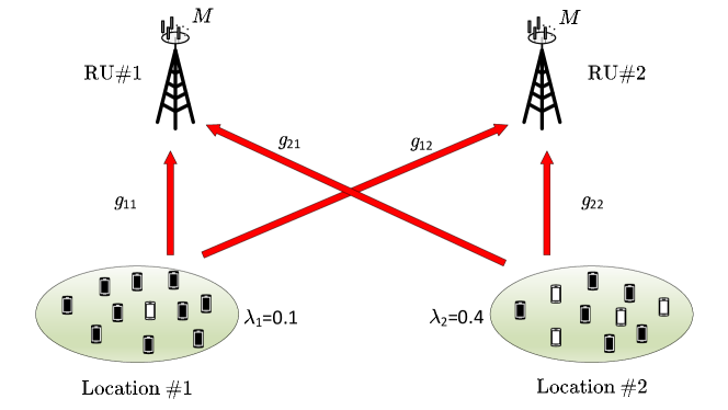
Figure 1: A toy model with $B=2$ and $U=2$ [1]. $g_{ub}$ denotes the large-scale fading coefficient between a user in $\mathcal{L}_{u}$ and the $M$ antenna array of RU $b$.

The random access users in location ${\cal L}_{u}$ are aware of their location and make use of the corresponding dictionary/codebook ${\bf S}_{u}$, i.e., any such user to transmit message $n\in[N_{u}]$, sends the corresponding codeword $\underline{{\bf s}}_{u,n}$ (i.e., the $n$-th column of ${\bf S}_{u}$). If the $(n,u)$ indexed message (i.e $n$th user in location ${\cal L}_{u}$) is transmitted, then ${\bf x}_{u,n}\sim{\bf h}_{u}$; otherwise, ${\bf x}_{u,n}={\mathchoice{\mbox{\boldmath$\displaystyle 0$}}{\mbox{\boldmath$\textstyle 0$}}{\mbox{\boldmath$\scriptstyle 0$}}{\mbox{\boldmath$\scriptscriptstyle 0$}}}$ (i.e. no transmission). Thus, we model

$${\bf X}_{u}\sim_{\text{i.i.d.}}a_{u}{\bf h}_{u},$$ (21)

where the random variable ${a}_{u}\sim\mathrm{Bern}(\lambda_{u})$ and random vector ${\bf h}_{u}\in\mathbb{C}^{F}$ are independent and associated with the random activity of the users and channel vectors at location ${\cal L}_{u}$, respectively.

For each $u\in[U]$, let $\widetilde{N}_{u}$ be the random number of active messages at location $u$, and let ${\bf D}_{u}\in\{0,1\}^{\tilde{N}_{u}\times N_{u}}$ be a projection matrix that removes zero rows from ${\bf X}_{u}$. We define

$$\underline{{\bf a}}_{u} \doteq\mathrm{diag}({\bf D}_{u}^{\top}{\bf D}_{u}).$$ (22)

$${\bf H}_{u} \doteq{\bf D}_{u}{\bf X}_{u}\;.$$ (23)

The goals of message detection and channel estimation are to infer the list of active messages (i.e., the binary vectors $\{\underline{{\bf a}}_{u}\}$) and the corresponding channels $\{{\bf H}_{u}\}$, respectively.

IV-A The Simplified Channel Model

While our analysis is generally applicable for any RV ${\bf h}_{u}\in\mathbb{C}^{F}$ with ${\bf h}_{u}=\mathcal{O}(1)$, it is important to develop an insightful fading model for ${\bf h}_{u}$. This is what we address in the sequel.

Let $g_{ub}$ stand for the large-scale fading coefficient (LSFC) between a user in $\mathcal{L}_{u}$ and the $M$ antenna array of RU $b$. We assume these coefficients are deterministic and known by the receiver. While in practice users are not perfectly co-located, and actual LSFCs will deviate slightly from the nominal values $\{g_{u,b}\}$, AMP theory can still be applied by appropriate constructions of the functions $f_{u,t}$. For further details, we refer the reader to [21] which also fully illustrates the effectiveness of the nominal LSFC assumption.

Second, we assume that the small-scale fading coefficients between any user and any RU antenna are i.i.d. $\sim{\cal C}{\cal N}(0,1)$ random variables (independent Rayleigh fading).

Consequently, the aggregated channel vector from a user in $\mathcal{L}_{u}$ to the $F=BM$ antennas of the RUs is a $1\times F$ Gaussian vector distributed as

$${\bf h}_{u}\equiv[{\bf h}_{u,1},{\bf h}_{u,2},\ldots,{\bf h}_{u,B}]\sim{\cal C}{\cal N}({\bf 0},{\mathchoice{\mbox{\boldmath$\displaystyle\Sigma$}}{\mbox{\boldmath$\textstyle\Sigma$}}{\mbox{\boldmath$\scriptstyle\Sigma$}}{\mbox{\boldmath$\scriptscriptstyle\Sigma$}}}_{u}),$$ (24)

where ${\mathchoice{\mbox{\boldmath$\displaystyle\Sigma$}}{\mbox{\boldmath$\textstyle\Sigma$}}{\mbox{\boldmath$\scriptstyle\Sigma$}}{\mbox{\boldmath$\scriptscriptstyle\Sigma$}}}_{u}$ is a $F\times F$ diagonal matrix given by

$${\mathchoice{\mbox{\boldmath$\displaystyle\Sigma$}}{\mbox{\boldmath$\textstyle\Sigma$}}{\mbox{\boldmath$\scriptstyle\Sigma$}}{\mbox{\boldmath$\scriptscriptstyle\Sigma$}}}_{u}\doteq{\rm diag}(g_{u,1},g_{u,2},\cdots,g_{u,B})\otimes{\bf I}_{M}\;.$$ (25)

IV-B Message Detection

From Theorem 1, we write for the last iteration $t=T$

$${\bf R}\simeq{\bf X}_{u}+{\mathchoice{\mbox{\boldmath$\displaystyle\Phi$}}{\mbox{\boldmath$\textstyle\Phi$}}{\mbox{\boldmath$\scriptstyle\Phi$}}{\mbox{\boldmath$\scriptscriptstyle\Phi$}}}_{u}$$ (26)

Here and throughout this section, we set ${\bf R}_{u}\equiv{\bf R}_{u}^{(T)}$, ${\mathchoice{\mbox{\boldmath$\displaystyle\Phi$}}{\mbox{\boldmath$\textstyle\Phi$}}{\mbox{\boldmath$\scriptstyle\Phi$}}{\mbox{\boldmath$\scriptscriptstyle\Phi$}}}_{u}\equiv{\mathchoice{\mbox{\boldmath$\displaystyle\Phi$}}{\mbox{\boldmath$\textstyle\Phi$}}{\mbox{\boldmath$\scriptstyle\Phi$}}{\mbox{\boldmath$\scriptscriptstyle\Phi$}}}_{u}^{(T)}$ and ${\bf C}_{\phi_{u}}\equiv{\bf C}_{\phi_{u}}^{(T,T)}$ for the sake of notational compactness. The high-dimensional representation (26) suggests that the following the detection rule [1]:

Definition 2 (Message detection).

We define the recovery of the binary message activity ${a}_{u,n}$ as

$${\widehat{a}}_{u,n}\doteq{\rm u}(\nu_{u}-\Lambda_{u}({\bf r}_{u,n}))\qquad\forall(u,n)\in[U]\times[N_{u}]$$ (27)

where ${\rm u}(\cdot)$ denotes the unit-step function and $\Lambda_{u}(\cdot)$ is decision-test function defined as

$$\Lambda_{u}({\bf r})\doteq\frac{\textswab{g}({\bf r}|{\bf 0},{\bf C}_{\phi_{u}})}{\int p_{u}({\bf h})\textswab{g}({\bf r}|{\bf h},{\bf C}_{\phi_{u}}){\rm d}{{\bf h}}}\;.$$ (28)

with $p_{u}({\bf h})$ denoting the density function of ${\bf h}_{u}$. Moreover, $\nu_{u}\in(0,\infty)$ is the decision threshold to achieve a desired trade-off between the missed detection and false alarm rates. $\lozenge$

Let us denote the actual set of active messages and the estimated set of active messages, respectively, as

$$\mathcal{A} \doteq\{(u,n)\in[U]\times[N_{u}]:a_{u,n}=1\}$$ (29)

$$\widehat{\mathcal{A}} \doteq\{(u,n)\in[U]\times[N_{u}]:\widehat{a}_{u,n}=1\}\;.$$ (30)

We then analyze the message detection in terms of the missed-detection and false-alarm rates which are denoted respectively,

$$\beta_{\rm e}^{\rm md} \doteq\frac{\big{|}{\widehat{\cal A}}^{\rm c}\cap{\cal A}\big{|}}{\big{|}{\cal A}\big{|}}$$ (31)

$$\beta_{\rm e}^{\rm fa} \doteq\frac{\big{|}\widehat{{\cal A}}\cap{\cal A}^{\rm c}\big{|}}{\big{|}{\cal A}^{\rm c}\big{|}}$$ (32)

where $\mathcal{B}^{\rm c}$ denotes the complement of the set $\mathcal{B}$. Here, and throughout the sequel, we use the subscripts $(\cdot)_{\rm e}$ and $(\cdot)_{\infty}$ in the notation to emphasize that the quantities are empirical and deterministic, respectively.

Assumption 2.

Let either the decision test function $\Lambda_{u}({\bf r})$ or its reciprocal, $1/\Lambda_{u}({\bf r})$, be Lipschitz continuous.

Suppose Assumption 2 and the premises of Theorem 1 hold. Then, following the identical steps of [1] we have as $L\to\infty$ that $\beta_{\rm e}^{\rm md}\overset{(a.s.)}{\rightarrow}\beta_{\infty}^{\rm md}$ and $\beta_{\rm e}^{\rm fa}\overset{(a.s.)}{\rightarrow}\beta_{\infty}^{\rm fa}$ where

$$\beta_{\infty}^{\rm md} \doteq\frac{1}{Z}\sum_{u\in[U]}\alpha_{u}\lambda_{u}\mathbb{P}(\Lambda_{u}({\bf h}_{u}+{\mathchoice{\mbox{\boldmath$\displaystyle\phi$}}{\mbox{\boldmath$\textstyle\phi$}}{\mbox{\boldmath$\scriptstyle\phi$}}{\mbox{\boldmath$\scriptscriptstyle\phi$}}}_{u})\geq\nu_{u})$$ (33)

$$\beta^{\rm fa}_{\infty} \doteq\frac{1}{\widetilde{Z}}\sum_{u\in[U]}\alpha_{u}(1-\lambda_{u})\mathbb{P}(\Lambda_{u}({\mathchoice{\mbox{\boldmath$\displaystyle\phi$}}{\mbox{\boldmath$\textstyle\phi$}}{\mbox{\boldmath$\scriptstyle\phi$}}{\mbox{\boldmath$\scriptscriptstyle\phi$}}}_{u})<\nu_{u})\;\;.$$ (34)

Here, ${\mathchoice{\mbox{\boldmath$\displaystyle\phi$}}{\mbox{\boldmath$\textstyle\phi$}}{\mbox{\boldmath$\scriptstyle\phi$}}{\mbox{\boldmath$\scriptscriptstyle\phi$}}}_{u}\sim\mathcal{CN}({\mathchoice{\mbox{\boldmath$\displaystyle 0$}}{\mbox{\boldmath$\textstyle 0$}}{\mbox{\boldmath$\scriptstyle 0$}}{\mbox{\boldmath$\scriptscriptstyle 0$}}},{\bf C}_{\phi_{u}})$ is independent of ${\bf h}_{u}$ and we define

$$Z\doteq\sum_{u\in[U]}\alpha_{u}\lambda_{u}~{}~{}\text{and}~{}~{}\widetilde{Z}\doteq\sum_{u\in[U]}\alpha_{u}(1-\lambda_{u})\;.$$ (35)

IV-C Channel Estimation

For short let $\eta_{u,T}(\cdot)\doteq\eta_{u}(\cdot)$. We then define the AMP channel estimation at the output of the last iteration (i.e. $t=T$)

$$\widehat{\bf h}_{u,n}=\eta_{u}({\bf r}_{u,n}),\quad(u,n)\in[U]\times[N_{u}]\;.$$ (36)

We partition $\widehat{{\cal A}}$ in two disjoint sets: those that are genuinely active and those that are inactive (false-alarm events):

$$\mathcal{A}^{\rm d}\doteq\widehat{{\cal A}}\cap{\cal A}~{}~{}\text{and}~{}~{}\mathcal{A}^{\rm fa}\doteq\widehat{{\cal A}}\cap{\cal A}^{c}\;.$$ (37)

From an operational viewpoint, channel estimation error matters only for messages in set $\mathcal{A}^{\rm d}$, as these correspond to users intending to access the network. In contrast, messages in $\mathcal{A}^{\rm fa}$ do not correspond to any real user, making their channel estimate quality irrelevant. However, false-alarm events (messages in $\mathcal{A}^{\rm fa}$) trigger the transmission of an ACK message in the DL, consuming some RU transmit power and causing multiuser interference to legitimate users. Therefore, we analyze the channel estimator in terms of the empirical averages of the mean-square-error for channels in $\mathcal{A}^{\rm d}$ and the powers consumed for the false alarm rates:

$${\rm mse}_{\rm e}^{\rm d} \doteq\frac{1}{|\mathcal{A}^{\rm d}|}\sum_{(u,n)\in\mathcal{A}^{\rm d}}\|{\bf h}_{u,n}-\widehat{\bf h}_{u,n}\|^{2}$$ (38)

$${\rm pow}_{\rm e}^{\rm fa} \doteq\frac{1}{|\mathcal{A}^{\rm fa}|}\sum_{(u,n)\in\mathcal{A}^{\rm fa}}\|\widehat{\bf h}_{u,n}\|^{2}\;.$$ (39)

Suppose Assumption (2) and the premises of Theorem 1 hold. Then, following the identical steps of [1] we have as $L\to\infty$ that ${\rm mse}_{\rm e}^{\rm d}\overset{(a.s.)}{\rightarrow}{\rm mse}_{\infty}^{\rm d}$ and ${\rm pow}_{\rm e}^{\rm fa}\overset{(a.s.)}{\rightarrow}{\rm pow}_{\infty}^{\rm fa}$ where we define

$${\rm mse}_{\infty}^{\rm d} \doteq\sum_{u\in U}\frac{\alpha_{u}\lambda_{u}\mathbb{P}(\mathcal{D}_{u})}{Z(1-\beta_{\infty}^{\rm md})}\mathbb{E}\left[\|{\bf h}_{u}-\eta_{u}({\bf h}_{u}+{\mathchoice{\mbox{\boldmath$\displaystyle\phi$}}{\mbox{\boldmath$\textstyle\phi$}}{\mbox{\boldmath$\scriptstyle\phi$}}{\mbox{\boldmath$\scriptscriptstyle\phi$}}}_{u})\|^{2}|\mathcal{D}_{u}\right]$$ (40)

$$\ {\rm pow}^{\rm fa}_{\infty} \doteq\sum_{u\in U}\frac{\alpha_{u}(1-\lambda_{u})\mathbb{P}(\mathcal{F}_{u})}{\widetilde{Z}\beta_{\infty}^{\rm fa}}\mathbb{E}\left[\|\eta_{u}({\mathchoice{\mbox{\boldmath$\displaystyle\phi$}}{\mbox{\boldmath$\textstyle\phi$}}{\mbox{\boldmath$\scriptstyle\phi$}}{\mbox{\boldmath$\scriptscriptstyle\phi$}}}_{u})\|^{2}|\mathcal{F}_{u}\right]$$ (41)

where ${\mathchoice{\mbox{\boldmath$\displaystyle\phi$}}{\mbox{\boldmath$\textstyle\phi$}}{\mbox{\boldmath$\scriptstyle\phi$}}{\mbox{\boldmath$\scriptscriptstyle\phi$}}}_{u}\sim\mathcal{CN}({\mathchoice{\mbox{\boldmath$\displaystyle 0$}}{\mbox{\boldmath$\textstyle 0$}}{\mbox{\boldmath$\scriptstyle 0$}}{\mbox{\boldmath$\scriptscriptstyle 0$}}},{\bf C}_{\phi_{u}})$ is independent of ${\bf h}_{u}$ and we define the events

$${\cal D}_{u} \doteq\{{\mathchoice{\mbox{\boldmath$\displaystyle\phi$}}{\mbox{\boldmath$\textstyle\phi$}}{\mbox{\boldmath$\scriptstyle\phi$}}{\mbox{\boldmath$\scriptscriptstyle\phi$}}}_{u},{\bf h}_{u}\in\mathbb{C}^{1\times F}:\Lambda_{u}({\bf h}_{u}+{\mathchoice{\mbox{\boldmath$\displaystyle\phi$}}{\mbox{\boldmath$\textstyle\phi$}}{\mbox{\boldmath$\scriptstyle\phi$}}{\mbox{\boldmath$\scriptscriptstyle\phi$}}}_{u})\leq\nu_{u}\}$$ (42)

$${\cal F}_{u} \doteq\{{\mathchoice{\mbox{\boldmath$\displaystyle\phi$}}{\mbox{\boldmath$\textstyle\phi$}}{\mbox{\boldmath$\scriptstyle\phi$}}{\mbox{\boldmath$\scriptscriptstyle\phi$}}}_{u}\in\mathbb{C}^{1\times F}:\Lambda_{u}({\mathchoice{\mbox{\boldmath$\displaystyle\phi$}}{\mbox{\boldmath$\textstyle\phi$}}{\mbox{\boldmath$\scriptstyle\phi$}}{\mbox{\boldmath$\scriptscriptstyle\phi$}}}_{u})<\nu_{u}\}\;$$ (43)

IV-D Genie-Aided MMSE Channel Estimation

In the low missed detection regime, i.e. $\beta^{\rm md}_{\infty}\ll 1$, it would be interesting to compare the asymptotic channel estimation error (40) with the asymptotic of so-called genie-aided MMSE, i.e., the exact MMSE conditioned on the knowledge of the true active messages ${\cal A}$:

$${\rm mmse}^{\rm genie}_{\rm e}\doteq\frac{1}{|\mathcal{A}|}{\left\|{\bf H}-\mathbb{E}[{\bf H}|{\bf Y},\{{\bf S}_{u}\},{\cal A}]\right\|_{\rm F}^{2}}$$ (44)

where for short we write ${\bf H}\equiv[{\bf H}_{1}^{\top},{\bf H}_{2}^{\top},\ldots,{\bf H}_{U}^{\top}]^{\top}$. In particular, for the motivated fading model in (24), we can use standard random-matrix theory arguments to derive the asymptotic expression of ${\rm mmse}_{\rm e}^{\rm genie}$. Specifically, let ${\bf N}\sim_{\text{i.i.d}}{\cal N}({\bf 0},\sigma^{2}{\bf I})$ and ${\bf H}_{u}\sim_{\text{i.i.d}}{\cal N}({\bf 0},{\mathchoice{\mbox{\boldmath$\displaystyle\Sigma$}}{\mbox{\boldmath$\textstyle\Sigma$}}{\mbox{\boldmath$\scriptstyle\Sigma$}}{\mbox{\boldmath$\scriptscriptstyle\Sigma$}}}_{u})$ with ${\mathchoice{\mbox{\boldmath$\displaystyle\Sigma$}}{\mbox{\boldmath$\textstyle\Sigma$}}{\mbox{\boldmath$\scriptstyle\Sigma$}}{\mbox{\boldmath$\scriptscriptstyle\Sigma$}}}_{u}={\rm diag}(\tau_{u1},\tau_{u2},\cdots,\tau_{uF})$ for each $u\in[U]$. Then, following the steps of [1, Appendix J], we get ${\rm mmse}_{\rm e}^{\rm genie}\overset{(a.s.)}{\rightarrow}{\rm mmse}^{\rm genie}_{\infty}$ where we define

$${\rm mmse}^{\rm genie}_{\infty}\doteq\frac{1}{Z}\sum_{(u,f)\in[U]\times[F]}\tau_{uf}\left(\alpha_{u}\lambda_{u}-\frac{\tau_{uf}}{c^{\star}_{f}}{\rm R}_{{\bf G}_{u}}(-\frac{\tau_{uf}}{c^{\star}_{f}})\right)\;.$$ (45)

Here, $c^{\star}_{f}$ is the unique solution of

$${c^{\star}_{f}}=\sigma^{2}+\sum_{u\in[U]}\tau_{uf}{\rm R}_{{\bf G}_{u}}(-\frac{\tau_{uf}}{c^{\star}_{f}})$$ (46)

and ${\rm\rm R}_{{\bf G}_{u}}$ denotes the R-transform of the limiting spectral distribution of ${\bf G}_{u}\equiv{\bf S}_{u}{\bf D}_{u}{\bf D}_{u}^{\top}{\bf S}_{u}^{\dagger}$ with ${\bf D}_{u}$ as in (22) and it reads as [22]

$${\rm R}_{{\bf G}_{u}}(x)=\frac{\alpha_{u}}{2x}\left((x-1)+\sqrt{(x-1)^{2}+4\lambda_{u}x}\right)\;.$$ (47)

IV-E Simulation Results

The simulations are based on the fading model in (24), i.e., ${\bf h}_{u}\sim{\cal N}({\mathchoice{\mbox{\boldmath$\displaystyle 0$}}{\mbox{\boldmath$\textstyle 0$}}{\mbox{\boldmath$\scriptstyle 0$}}{\mbox{\boldmath$\scriptscriptstyle 0$}}},{\mathchoice{\mbox{\boldmath$\displaystyle\Sigma$}}{\mbox{\boldmath$\textstyle\Sigma$}}{\mbox{\boldmath$\scriptstyle\Sigma$}}{\mbox{\boldmath$\scriptscriptstyle\Sigma$}}}_{u})$ and ${\mathchoice{\mbox{\boldmath$\displaystyle\Sigma$}}{\mbox{\boldmath$\textstyle\Sigma$}}{\mbox{\boldmath$\scriptstyle\Sigma$}}{\mbox{\boldmath$\scriptscriptstyle\Sigma$}}}_{u}={\rm diag}(g_{u,1},g_{u,2},\cdots,g_{u,B})\otimes{\bf I}_{M}$ and Gaussian noise as ${\bf N}\sim_{\text{i.i.d.}}{\cal N}({\mathchoice{\mbox{\boldmath$\displaystyle 0$}}{\mbox{\boldmath$\textstyle 0$}}{\mbox{\boldmath$\scriptstyle 0$}}{\mbox{\boldmath$\scriptscriptstyle 0$}}},\sigma^{2}{\bf I}_{F})$. Furthermore, we consider a $2$-location toy example with $U=B=2$ locations and RUs—similar to ”symmetric” adjacent cell interference model as “Wyner model” [23, 24]—as depicted in Fig. 1. The corresponding $2\times 2$ LSFC matrix is defined as:

$$[g_{ub}]=\begin{bmatrix}1&\wp\\ \wp&1\end{bmatrix}$$

where $\wp\in[0,1]$ denotes the crosstalk coefficient between location $u$ and RU $b\neq u$. In our simulations, we set $\wp=\frac{1}{2}$.

To assess the impact of the number of locations, we extend the toy example to include 4 locations, configured such that $\lambda_{1}=\lambda_{3}$, $\lambda_{2}=\lambda_{4}$, ${\mathchoice{\mbox{\boldmath$\displaystyle\Sigma$}}{\mbox{\boldmath$\textstyle\Sigma$}}{\mbox{\boldmath$\scriptstyle\Sigma$}}{\mbox{\boldmath$\scriptscriptstyle\Sigma$}}}_{1}={\mathchoice{\mbox{\boldmath$\displaystyle\Sigma$}}{\mbox{\boldmath$\textstyle\Sigma$}}{\mbox{\boldmath$\scriptstyle\Sigma$}}{\mbox{\boldmath$\scriptscriptstyle\Sigma$}}}_{3}$, and ${\mathchoice{\mbox{\boldmath$\displaystyle\Sigma$}}{\mbox{\boldmath$\textstyle\Sigma$}}{\mbox{\boldmath$\scriptstyle\Sigma$}}{\mbox{\boldmath$\scriptscriptstyle\Sigma$}}}_{2}={\mathchoice{\mbox{\boldmath$\displaystyle\Sigma$}}{\mbox{\boldmath$\textstyle\Sigma$}}{\mbox{\boldmath$\scriptstyle\Sigma$}}{\mbox{\boldmath$\scriptscriptstyle\Sigma$}}}_{4}$, where ${\mathchoice{\mbox{\boldmath$\displaystyle\Sigma$}}{\mbox{\boldmath$\textstyle\Sigma$}}{\mbox{\boldmath$\scriptstyle\Sigma$}}{\mbox{\boldmath$\scriptscriptstyle\Sigma$}}}_{1}$ and ${\mathchoice{\mbox{\boldmath$\displaystyle\Sigma$}}{\mbox{\boldmath$\textstyle\Sigma$}}{\mbox{\boldmath$\scriptstyle\Sigma$}}{\mbox{\boldmath$\scriptscriptstyle\Sigma$}}}_{2}$ are as in the original 2-location toy example.

In Figure 3 and Figure 3,

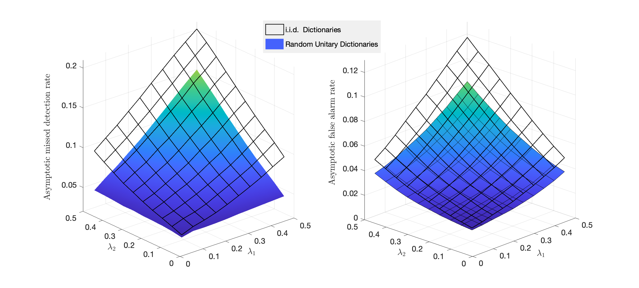
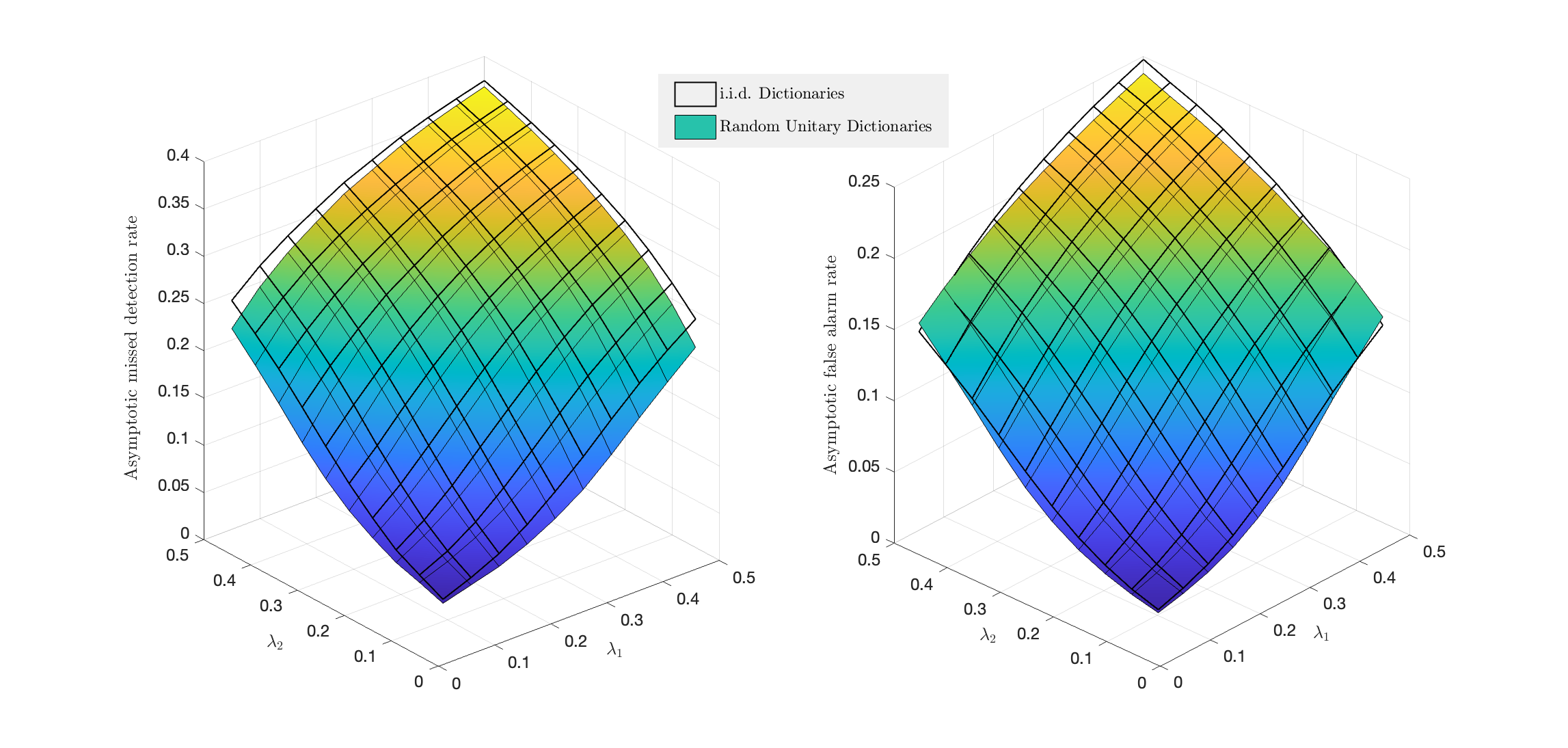
Figure 2: $2$-Locations: Comparison of asymptotic missed detection and false alarm rates with $\alpha_{u}=1$ and $\sigma^{2}=0.1$.

Figure 3: $4$ Locations: Comparison of asymptotic missed detection and false alarm rates with $\alpha_{u}=1$ and $\sigma^{2}=0.1$.

we compare the asymptotic missed detection and false alarm rates for the $2$-Location and $4$-Location examples, respectively. These rates are evaluated for both i.i.d. Gaussian dictionaries [1, Theorem 2] and random unitary dictionaries as in (33)-(34). We focus on the special case where $\alpha_{u}=L$, i.e., the $U$-Orthogonal model [17]. The results show that for the $2$-Location example as system sparsity decreases, random unitary dictionaries provide significantly better performance. However, increasing the number of locations to $4$ results in only a negligible difference in performance.

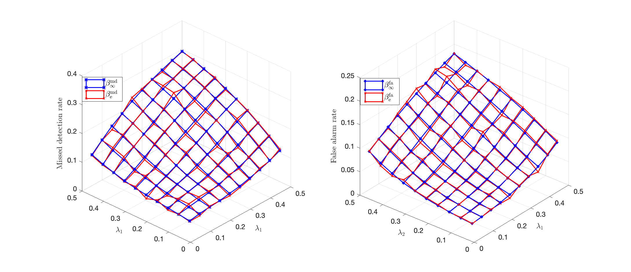
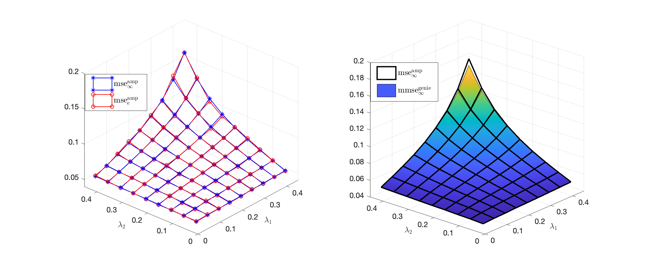
Figure 4: Randomly-signed Fourier dictionaries: 2-Locations, $L=2^{13}$, $\alpha_{u}=\frac{3}{2}$, and $\sigma^{2}=0.1$. Simulations for each pair $(\lambda_{1},\lambda_{2})$ are based on a single, independent instance of the AMP dynamics.

Figure 5: 2-Locations with $\alpha_{u}=1$ and $\sigma^{2}=10^{-2}$: (Left) Theory-simulation discrepancy with $L=2^{13}$ and randomly-signed Fourier dictionaries where for each pair $(\lambda_{1},\lambda_{2})$ are based on a single, independent instance of the AMP dynamics; (Right) Comparison with the asymptotic AMP channel estimation error and the genie-aided MMSE.

As to the conjecture outlined in Section III, we construct dictionaries using randomly-signed Fourier matrices (instead of Haar unitary matrices) as described in (20) and compare in Figure 5 both the missed detection rate $\beta_{\rm e}^{\rm md}$ and false alarm rate $\beta_{\rm e}^{\rm fa}$ with the theoretical quantities $\beta^{\rm md}_{\infty}$ and $\beta^{\rm fa}_{\infty}$, respectively.

Finally, Figure 5 illustrates the channel estimation results. Note that these results are based on a reduced noise variance $\sigma^{2}=10^{-2}$ (instead of $\sigma^{2}=10^{-1}$), leading to low miss-detection rates. Indeed, the asymptotic AMP channel estimation error closely matches the asymptotic genie-aided MMSE.

V Conclusion and Outlook

Following [1], we address the inference problem for matrix-valued noisy linear observations involving multiple statistically asymmetric signal sources. Instead of assuming that dictionaries for each signal source are drawn from an i.i.d. (Gaussian) random matrix ensemble as in [1], we consider the novel assumption of random semi-unitary dictionaries. Accordingly, we have developed a new AMP algorithm and provided its high-dimensional analysis.

As a proof of concept, we apply our theory to the problem of joint message detection and channel estimation in unsourced random access for cell-free wireless networks.

Proving the conjecture outlined in Section III—specifically, Theorem 1 using dictionary matrices constructed from randomly signed Fourier matrices—constitutes a significant theoretical contribution. Additionally, extending the framework to accommodate general bi-unitarily invariant dictionary matrices [25] represents an intriguing direction for future research, potentially covering a wide range of relevant applications. However, this extension would require singular value decomposition for each dictionary matrix, which poses a computational challenge. However, we expect that the memory-AMP approach [26] could resolve this issue.

Appendix A The Proof of Theorem 1

It is useful to define the residuals for all $(u,t)\in[U]\times[T]$

$$\widehat{{\mathchoice{\mbox{\boldmath$\displaystyle\Psi$}}{\mbox{\boldmath$\textstyle\Psi$}}{\mbox{\boldmath$\scriptstyle\Psi$}}{\mbox{\boldmath$\scriptscriptstyle\Psi$}}}}_{u}^{(t)} \doteq{\mathchoice{\mbox{\boldmath$\displaystyle\Gamma$}}{\mbox{\boldmath$\textstyle\Gamma$}}{\mbox{\boldmath$\scriptstyle\Gamma$}}{\mbox{\boldmath$\scriptscriptstyle\Gamma$}}}_{u}^{(t)}-{\mathchoice{\mbox{\boldmath$\displaystyle\Theta$}}{\mbox{\boldmath$\textstyle\Theta$}}{\mbox{\boldmath$\scriptstyle\Theta$}}{\mbox{\boldmath$\scriptscriptstyle\Theta$}}}_{u}$$ (48)

$$\widehat{{\mathchoice{\mbox{\boldmath$\displaystyle\Phi$}}{\mbox{\boldmath$\textstyle\Phi$}}{\mbox{\boldmath$\scriptstyle\Phi$}}{\mbox{\boldmath$\scriptscriptstyle\Phi$}}}}_{u}^{(t)} \doteq{\bf R}_{u}^{(t)}-{\bf X}_{u}\;.$$ (49)

Then, from (50), we have the recursion for $t=1,2,\cdots,T$

$$\widehat{{\mathchoice{\mbox{\boldmath$\displaystyle\Psi$}}{\mbox{\boldmath$\textstyle\Psi$}}{\mbox{\boldmath$\scriptstyle\Psi$}}{\mbox{\boldmath$\scriptscriptstyle\Psi$}}}}_{u}^{(t)} =\sqrt{\alpha_{u}}{\bf O}_{u}{\bf T}_{u}^{(t)}$$ (50a)

$${\bf Z}^{(t)} ={\bf N}-\sum_{u\leq U}{\bf P}_{u}\widehat{{\mathchoice{\mbox{\boldmath$\displaystyle\Psi$}}{\mbox{\boldmath$\textstyle\Psi$}}{\mbox{\boldmath$\scriptstyle\Psi$}}{\mbox{\boldmath$\scriptscriptstyle\Psi$}}}}_{u}^{(t)}$$ (50b)

$$\widetilde{{\bf T}}_{u}^{(t)} =\sqrt{\alpha_{u}}{\bf P}_{u}^{\top}{\bf Z}^{(t)}$$ (50c)

$$\widehat{{\mathchoice{\mbox{\boldmath$\displaystyle\Phi$}}{\mbox{\boldmath$\textstyle\Phi$}}{\mbox{\boldmath$\scriptstyle\Phi$}}{\mbox{\boldmath$\scriptscriptstyle\Phi$}}}}_{u}^{(t)} ={\bf O}_{u}^{\dagger}\widetilde{{\bf T}}_{u}^{(t)}+{\bf T}_{u}^{(t)}\;$$ (50d)

$${\bf T}_{u}^{(t+1)} ={f}_{u,t}({\bf X}_{u}+\widehat{{\mathchoice{\mbox{\boldmath$\displaystyle\Phi$}}{\mbox{\boldmath$\textstyle\Phi$}}{\mbox{\boldmath$\scriptstyle\Phi$}}{\mbox{\boldmath$\scriptscriptstyle\Phi$}}}}_{u}^{(t)})-{\bf X}_{u}$$ (50e)

with the initialization ${{\bf T}}_{u}^{(1)}\doteq{\bf F}_{u}^{(1)}-{\bf X}_{u}$. Hence, for the proof, it is sufficient to verify

$$\widehat{{\mathchoice{\mbox{\boldmath$\displaystyle\Psi$}}{\mbox{\boldmath$\textstyle\Psi$}}{\mbox{\boldmath$\scriptstyle\Psi$}}{\mbox{\boldmath$\scriptscriptstyle\Psi$}}}}_{u}^{(t)} \simeq{{\mathchoice{\mbox{\boldmath$\displaystyle\Psi$}}{\mbox{\boldmath$\textstyle\Psi$}}{\mbox{\boldmath$\scriptstyle\Psi$}}{\mbox{\boldmath$\scriptscriptstyle\Psi$}}}}_{u}^{(t)}$$ (51)

$$\widehat{{\mathchoice{\mbox{\boldmath$\displaystyle\Phi$}}{\mbox{\boldmath$\textstyle\Phi$}}{\mbox{\boldmath$\scriptstyle\Phi$}}{\mbox{\boldmath$\scriptscriptstyle\Phi$}}}}_{u}^{(t)} \simeq{\mathchoice{\mbox{\boldmath$\displaystyle\Phi$}}{\mbox{\boldmath$\textstyle\Phi$}}{\mbox{\boldmath$\scriptstyle\Phi$}}{\mbox{\boldmath$\scriptscriptstyle\Phi$}}}_{u}^{(t)}\;.$$ (52)

At a high level, the proof consists of two main steps. In the first step (Section A-A), we mimic the idea of the so-called “Householder dice” representation of AMP-type dynamics coupled by a Haar matrix [27, Section III-C] and construct an ${\bf O}_{u}$-free equivalent dynamics of (50). In the second step (Section A-B), we follow the similar steps of [1, Section B.2] and derive the high-dimensional representation of the random matrix-free dynamics, which will give us the high-dimensional equivalent of the original AMP dynamics.

For convenience, we will use the following notation for matrices throughout the proof: Let the matrices ${\bf A}$ and ${\bf B}$ have the same number of rows, denoted by $N$. Then, we define

$$\langle{\bf A},{\bf B}\rangle\doteq\frac{1}{N}{\bf A}^{\dagger}{\bf B}$$ (53)

whenever the dependency on $N$ is clear from the context.

A-A The Random-Matrix-Free Equivalent

We fix the update rules in (50b)-(50c) and (50e) and derive the ${\bf O}_{u}$-free representations of ${\bf O}_{u}{\bf T}_{u}^{(t)}$ and ${\bf O}_{u}^{\dagger}\widetilde{\bf T}_{u}^{(t)}$. For convenience, we fix $u\in[U]$ and remove the subscript $u$ from the notation, e.g. $N\equiv N_{u}$, ${\bf O}\equiv{\bf O}_{u}$, ${\bf T}^{(t)}\equiv{\bf T}_{u}^{(t)}$, etc.

We begin with the block Gram-Schmidt notation: Let ${\bf V}^{(1:t-1)}=\{{\bf V}^{(1)},{\bf V}^{(2)},\ldots,{\bf V}^{(t-1)}\}$ be set of $N\times F$ matrices with $\langle{\bf V}^{(i)},{\bf V}^{(j)}\rangle=\mathcal{\delta}_{ij}{\bf I}_{F}$ for all $i,j$. Then, for any matrix ${\bf B}\in\mathbb{C}^{N\times F}$, by using the block Gram-Schmidt (orthogonalization) process, we can always construct the new (semi-unitary) matrix

$${\bf V}^{(t)}\stackrel{{\scriptstyle\Delta}}{{=}}\mathcal{GS}({\bf B}\mid{\bf V}^{(1:t-1)})$$

such that $\langle{\bf V}^{(t)},{\bf V}^{(s)}\rangle=\delta_{st}{\bf I}_{F}$ and we have the block Gram-Schmidt decomposition

$${\bf B}=\sum_{1\leq s\leq t}{\bf V}^{(s)}\langle{\bf V}^{(s)},{\bf B}\rangle\;.$$ (54)

We also refer to [1, Appendix L] for an explicit definition of the (block) Gram-Schmidt notation. Furthermore, we note that for the projection matrix

$${\bf P}^{\perp}_{{\bf V}^{(1:t-1)}}\doteq{\bf I}-\frac{1}{N}\sum_{1\leq s<t}{\bf V}^{(s)}({\bf V}^{(s)})^{\dagger}\;$$ (55)

if the matrix ${\bf Q}\doteq{\bf B}^{\dagger}{\bf P}^{\perp}_{{\bf V}^{(1:t-1)}}{\bf B}$ is singular then the Gram-Schmidt process is unique and it is given by

$${\bf V}^{(t)}\equiv\sqrt{N}{\bf P}^{\perp}_{{\bf V}^{(1:t-1)}}{\bf B}{\bf Q}^{-\frac{1}{2}}\;.$$ (56)

In particular, when ${\bf B}\sim_{\text{i.i.d.}}\mathcal{CN}({\mathchoice{\mbox{\boldmath$\displaystyle 0$}}{\mbox{\boldmath$\textstyle 0$}}{\mbox{\boldmath$\scriptstyle 0$}}{\mbox{\boldmath$\scriptscriptstyle 0$}}},{\bf I}_{F})$, we have ${\bf Q}\sim\widetilde{\bf B}^{\dagger}\widetilde{\bf B}$ where $\widetilde{\bf B}\in\mathbb{C}^{(N-(t-1)F)\times F}$ and $\widetilde{\bf B}\sim_{\text{i.i.d.}}\mathcal{CN}({\mathchoice{\mbox{\boldmath$\displaystyle 0$}}{\mbox{\boldmath$\textstyle 0$}}{\mbox{\boldmath$\scriptstyle 0$}}{\mbox{\boldmath$\scriptscriptstyle 0$}}},{\bf I}_{F})$; thereby the Gram-Schmidt process is (a.s.) unique when $N\geq Ft$.

We will adaptively use the following representation of the Haar unitary matrix.

Lemma 1.

Let the random elements $\widetilde{\bf G}^{(1)},{\bf V}^{(1)}\in\mathbb{C}^{N\times F}$ and the random matrix ${{\bf O}^{(N-F)}}\in\mathbb{C}^{(N-F)\times(N-F)}$ be mutually independent. Let $\widetilde{\bf G}^{(1)}\sim_{\text{i.i.d.}}\mathcal{CN}({\mathchoice{\mbox{\boldmath$\displaystyle 0$}}{\mbox{\boldmath$\textstyle 0$}}{\mbox{\boldmath$\scriptstyle 0$}}{\mbox{\boldmath$\scriptscriptstyle 0$}}},{\bf I}_{F})$, $\langle{\bf V}^{(1)},{\bf V}^{(1)}\rangle={\bf I}_{F}$ and ${{\bf O}^{(N-F)}}$ is Haar unitary. Then, for $\widetilde{\bf V}^{(1)}\doteq\mathcal{GS}(\widetilde{\bf G}^{(1)})$, the matrix

$${\bf O} \doteq\frac{1}{N}\widetilde{\bf V}^{(1)}({\bf V}^{(1)})^{\dagger}+{\mathchoice{\mbox{\boldmath$\displaystyle\Pi$}}{\mbox{\boldmath$\textstyle\Pi$}}{\mbox{\boldmath$\scriptstyle\Pi$}}{\mbox{\boldmath$\scriptscriptstyle\Pi$}}}_{\widetilde{\bf V}^{(1)}}^{\perp}{\bf O}^{(N-F)}({\mathchoice{\mbox{\boldmath$\displaystyle\Pi$}}{\mbox{\boldmath$\textstyle\Pi$}}{\mbox{\boldmath$\scriptstyle\Pi$}}{\mbox{\boldmath$\scriptscriptstyle\Pi$}}}_{{\bf V}^{(1)}}^{\perp})^{\dagger}$$ (57)

is Haar unitary and independent of ${\bf V}^{(1)}$. Here, we introduce the semi-unitary matrices ${\mathchoice{\mbox{\boldmath$\displaystyle\Pi$}}{\mbox{\boldmath$\textstyle\Pi$}}{\mbox{\boldmath$\scriptstyle\Pi$}}{\mbox{\boldmath$\scriptscriptstyle\Pi$}}}_{\widetilde{\bf V}^{(1)}}^{\perp},{\mathchoice{\mbox{\boldmath$\displaystyle\Pi$}}{\mbox{\boldmath$\textstyle\Pi$}}{\mbox{\boldmath$\scriptstyle\Pi$}}{\mbox{\boldmath$\scriptscriptstyle\Pi$}}}_{{\bf V}^{(1)}}^{\perp}\in\mathbb{C}^{N\times(N-F)}$ whose columns spanning the orthogonal complements of the column spans of $\widetilde{\bf V}^{(1)}$ and ${\bf V}^{(1)}$, respectively. E.g., we have

$${\mathchoice{\mbox{\boldmath$\displaystyle\Pi$}}{\mbox{\boldmath$\textstyle\Pi$}}{\mbox{\boldmath$\scriptstyle\Pi$}}{\mbox{\boldmath$\scriptscriptstyle\Pi$}}}_{{\bf V}^{(1)}}^{\perp}({\mathchoice{\mbox{\boldmath$\displaystyle\Pi$}}{\mbox{\boldmath$\textstyle\Pi$}}{\mbox{\boldmath$\scriptstyle\Pi$}}{\mbox{\boldmath$\scriptscriptstyle\Pi$}}}_{{\bf V}^{(1)}}^{\perp})^{\dagger}={\bf I}-\frac{1}{N}{\bf V}^{(1)}({\bf V}^{(1)})^{\dagger}={\bf P}_{{\bf V}^{(1)}}^{\perp}.$$

Proof.

For the case $F=1$, the proof of can be obtained by following the arguments of the proof of [27, Lemma 1]. The extension to arbitrary $F>1$ is analogous. ∎

Let ${\bf V}^{(1)}\equiv\mathcal{GS}({{\bf T}^{(1)}})$, so that we get from Lemma 1

$${\bf O}{\bf T}^{(1)}=\widetilde{\bf V}^{(1)}\langle{\bf V}^{(1)},{\bf T}^{(1)}\rangle.$$ (58)

The form of representation (57) is useful for the multiplications of the Haar matrix from the right, e.g. ${\bf O}{\bf T}^{(1)}$. To treat the multiplication from left such as ${\bf O}^{\dagger}\widetilde{\bf T}^{(1)}$, we introduce a new arbitrary Gaussian element ${\bf G}^{(1)}\sim_{\text{i.i.d.}}\mathcal{CN}({\mathchoice{\mbox{\boldmath$\displaystyle 0$}}{\mbox{\boldmath$\textstyle 0$}}{\mbox{\boldmath$\scriptstyle 0$}}{\mbox{\boldmath$\scriptscriptstyle 0$}}},{\bf I}_{F})$ with noting that

$$({\mathchoice{\mbox{\boldmath$\displaystyle\Pi$}}{\mbox{\boldmath$\textstyle\Pi$}}{\mbox{\boldmath$\scriptstyle\Pi$}}{\mbox{\boldmath$\scriptscriptstyle\Pi$}}}_{{\bf V}^{(1)}}^{\perp})^{\dagger}{\bf G}^{(1)}\sim_{\text{i.i.d.}}\mathcal{CN}({\mathchoice{\mbox{\boldmath$\displaystyle 0$}}{\mbox{\boldmath$\textstyle 0$}}{\mbox{\boldmath$\scriptstyle 0$}}{\mbox{\boldmath$\scriptscriptstyle 0$}}},{\bf I}_{F})$$

and it is independent of ${\bf V}^{(1)}$. Let $\widetilde{\bf V}^{(2)}\equiv\mathcal{GS}(\widetilde{\bf T}^{(1)}\mid\widetilde{\bf V}^{(1)})$. Then, by using Lemma 1, we represent ${\bf O}^{(N-F)}$ in (57) as

$${\bf O}^{(N-F)} =\frac{1}{N}\mathcal{GS}(({\mathchoice{\mbox{\boldmath$\displaystyle\Pi$}}{\mbox{\boldmath$\textstyle\Pi$}}{\mbox{\boldmath$\scriptstyle\Pi$}}{\mbox{\boldmath$\scriptscriptstyle\Pi$}}}_{\widetilde{\bf V}^{(1)}}^{\perp})^{\dagger}\widetilde{\bf V}^{(2)})\mathcal{GS}(({\mathchoice{\mbox{\boldmath$\displaystyle\Pi$}}{\mbox{\boldmath$\textstyle\Pi$}}{\mbox{\boldmath$\scriptstyle\Pi$}}{\mbox{\boldmath$\scriptscriptstyle\Pi$}}}_{{\bf V}^{(1)}}^{\perp})^{\dagger}{\bf G}^{(1)})^{\dagger}$$

$$+{\mathchoice{\mbox{\boldmath$\displaystyle\Pi$}}{\mbox{\boldmath$\textstyle\Pi$}}{\mbox{\boldmath$\scriptstyle\Pi$}}{\mbox{\boldmath$\scriptscriptstyle\Pi$}}}_{({\mathchoice{\mbox{\boldmath$\displaystyle\Pi$}}{\mbox{\boldmath$\textstyle\Pi$}}{\mbox{\boldmath$\scriptstyle\Pi$}}{\mbox{\boldmath$\scriptscriptstyle\Pi$}}}_{\widetilde{\bf V}^{(1)}}^{\perp})^{\dagger}\widetilde{\bf V}^{(2)}}^{\perp}{\bf O}^{(N-2F)}\left({\mathchoice{\mbox{\boldmath$\displaystyle\Pi$}}{\mbox{\boldmath$\textstyle\Pi$}}{\mbox{\boldmath$\scriptstyle\Pi$}}{\mbox{\boldmath$\scriptscriptstyle\Pi$}}}_{({\mathchoice{\mbox{\boldmath$\displaystyle\Pi$}}{\mbox{\boldmath$\textstyle\Pi$}}{\mbox{\boldmath$\scriptstyle\Pi$}}{\mbox{\boldmath$\scriptscriptstyle\Pi$}}}_{{\bf V}^{(1)}}^{\perp})^{\dagger}{\bf G}^{(1)}}^{\perp}\right)^{\dagger}\;$$ (59)

where ${\bf O}^{N-2F}\in\mathbb{C}^{(N-2F)\times(N-2F)}$ is Haar unitary. Moreover, one can verify that

$${\mathchoice{\mbox{\boldmath$\displaystyle\Pi$}}{\mbox{\boldmath$\textstyle\Pi$}}{\mbox{\boldmath$\scriptstyle\Pi$}}{\mbox{\boldmath$\scriptscriptstyle\Pi$}}}_{\widetilde{\bf V}^{(1)}}^{\perp}\mathcal{GS}(({\mathchoice{\mbox{\boldmath$\displaystyle\Pi$}}{\mbox{\boldmath$\textstyle\Pi$}}{\mbox{\boldmath$\scriptstyle\Pi$}}{\mbox{\boldmath$\scriptscriptstyle\Pi$}}}_{\widetilde{\bf V}^{(1)}}^{\perp})^{\dagger}\widetilde{\bf V}^{(2)}) \equiv\widetilde{\bf V}^{(2)}$$ (60)

$${\mathchoice{\mbox{\boldmath$\displaystyle\Pi$}}{\mbox{\boldmath$\textstyle\Pi$}}{\mbox{\boldmath$\scriptstyle\Pi$}}{\mbox{\boldmath$\scriptscriptstyle\Pi$}}}_{{\bf V}^{(1)}}^{\perp}\mathcal{GS}(({\mathchoice{\mbox{\boldmath$\displaystyle\Pi$}}{\mbox{\boldmath$\textstyle\Pi$}}{\mbox{\boldmath$\scriptstyle\Pi$}}{\mbox{\boldmath$\scriptscriptstyle\Pi$}}}_{{\bf V}^{(1)}}^{\perp})^{\dagger}{\bf G}^{(1)}) =\underbrace{\mathcal{GS}({\bf G}^{(1)}\mid{\bf V}^{(1)})}_{\doteq{\bf V}^{(2)}}\;.$$ (61)

Hence, we get the representation

$${\bf O}=\frac{1}{N}\widetilde{\bf V}^{(1)}({\bf V}^{(1)})^{\dagger}+\frac{1}{N}\widetilde{\bf V}^{(2)}({\bf V}^{(2)})^{\dagger}$$

$$+\underbrace{\left({\mathchoice{\mbox{\boldmath$\displaystyle\Pi$}}{\mbox{\boldmath$\textstyle\Pi$}}{\mbox{\boldmath$\scriptstyle\Pi$}}{\mbox{\boldmath$\scriptscriptstyle\Pi$}}}_{\widetilde{\bf V}^{(1)}}^{\perp}{\mathchoice{\mbox{\boldmath$\displaystyle\Pi$}}{\mbox{\boldmath$\textstyle\Pi$}}{\mbox{\boldmath$\scriptstyle\Pi$}}{\mbox{\boldmath$\scriptscriptstyle\Pi$}}}_{({\mathchoice{\mbox{\boldmath$\displaystyle\Pi$}}{\mbox{\boldmath$\textstyle\Pi$}}{\mbox{\boldmath$\scriptstyle\Pi$}}{\mbox{\boldmath$\scriptscriptstyle\Pi$}}}_{\widetilde{\bf V}^{(1)}}^{\perp})^{\dagger}\widetilde{\bf V}^{(2)}}^{\perp}\right)}_{\doteq{\mathchoice{\mbox{\boldmath$\displaystyle\Pi$}}{\mbox{\boldmath$\textstyle\Pi$}}{\mbox{\boldmath$\scriptstyle\Pi$}}{\mbox{\boldmath$\scriptscriptstyle\Pi$}}}^{\perp}_{\widetilde{\bf V}^{(1:2)}}}{\bf O}^{(N-2F)}{\underbrace{\left({\mathchoice{\mbox{\boldmath$\displaystyle\Pi$}}{\mbox{\boldmath$\textstyle\Pi$}}{\mbox{\boldmath$\scriptstyle\Pi$}}{\mbox{\boldmath$\scriptscriptstyle\Pi$}}}_{{\bf V}^{(1)}}^{\perp}{\mathchoice{\mbox{\boldmath$\displaystyle\Pi$}}{\mbox{\boldmath$\textstyle\Pi$}}{\mbox{\boldmath$\scriptstyle\Pi$}}{\mbox{\boldmath$\scriptscriptstyle\Pi$}}}_{({\mathchoice{\mbox{\boldmath$\displaystyle\Pi$}}{\mbox{\boldmath$\textstyle\Pi$}}{\mbox{\boldmath$\scriptstyle\Pi$}}{\mbox{\boldmath$\scriptscriptstyle\Pi$}}}_{{\bf V}^{(1)}}^{\perp})^{\dagger}{\bf G}^{(1)}}^{\perp}\right)}_{\doteq{\mathchoice{\mbox{\boldmath$\displaystyle\Pi$}}{\mbox{\boldmath$\textstyle\Pi$}}{\mbox{\boldmath$\scriptstyle\Pi$}}{\mbox{\boldmath$\scriptscriptstyle\Pi$}}}^{\perp}_{{\bf V}^{(1:2)}}}}^{\dagger}\;.$$ (62)

Here, e.g. one can show from (61) that ${\mathchoice{\mbox{\boldmath$\displaystyle\Pi$}}{\mbox{\boldmath$\textstyle\Pi$}}{\mbox{\boldmath$\scriptstyle\Pi$}}{\mbox{\boldmath$\scriptscriptstyle\Pi$}}}^{\perp}_{{\bf V}^{(1:2)}}\in\mathbb{C}^{N\times(N-2F)}$ semi unitary matrix such that

$${\mathchoice{\mbox{\boldmath$\displaystyle\Pi$}}{\mbox{\boldmath$\textstyle\Pi$}}{\mbox{\boldmath$\scriptstyle\Pi$}}{\mbox{\boldmath$\scriptscriptstyle\Pi$}}}^{\perp}_{{\bf V}^{(1:2)}}({\mathchoice{\mbox{\boldmath$\displaystyle\Pi$}}{\mbox{\boldmath$\textstyle\Pi$}}{\mbox{\boldmath$\scriptstyle\Pi$}}{\mbox{\boldmath$\scriptscriptstyle\Pi$}}}^{\perp}_{{\bf V}^{(1:2)}})^{\dagger}={\bf P}^{\perp}_{{\bf V}^{(1:2)}}.$$ (63)

So that we get from (62)

$${\bf O}^{\dagger}\widetilde{\bf T}^{(1)}={\bf V}^{(1)}\langle\widetilde{\bf V}^{(1)},\widetilde{\bf T}^{(1)}\rangle+{\bf V}^{(2)}\langle\widetilde{\bf V}^{(2)},\widetilde{\bf T}^{(1)}\rangle\;.$$ (64)

Hence, we complete the ${\bf O}$-free representation of the AMP dynamics for the first iteration step $t=1$.

Moving on to the second iteration step, we fix $t=2$ but mimic the notations in a manner that the arguments can be recalled for any $t>1$. Firstly, we generate arbitrary i.i.d. Gaussian elements,

$$\widetilde{\bf G}^{(t)}\sim{\bf G}^{(t)}~{}\sim_{\text{i.i.d.}}\mathcal{CN}({\mathchoice{\mbox{\boldmath$\displaystyle 0$}}{\mbox{\boldmath$\textstyle 0$}}{\mbox{\boldmath$\scriptstyle 0$}}{\mbox{\boldmath$\scriptscriptstyle 0$}}},{\bf I}_{F})\;.$$

Second, we construct the basis

$${\bf V}^{(2t-1)} =\mathcal{GS}({\bf T}^{(t)}|{\bf V}^{(1:2(t-1))})$$ (65)

$$\widetilde{\bf V}^{(2t-1)} =\mathcal{GS}(\widetilde{\bf G}^{(t)}|\widetilde{\bf V}^{(1:2(t-1))})\;.$$ (66)

Notice that

$$({\mathchoice{\mbox{\boldmath$\displaystyle\Pi$}}{\mbox{\boldmath$\textstyle\Pi$}}{\mbox{\boldmath$\scriptstyle\Pi$}}{\mbox{\boldmath$\scriptscriptstyle\Pi$}}}_{\widetilde{\bf V}^{(1:2(t-1)}}^{\perp})^{\dagger}\widetilde{\bf G}^{(1)}\sim_{\text{i.i.d.}}\mathcal{CN}({\mathchoice{\mbox{\boldmath$\displaystyle 0$}}{\mbox{\boldmath$\textstyle 0$}}{\mbox{\boldmath$\scriptstyle 0$}}{\mbox{\boldmath$\scriptscriptstyle 0$}}},{\bf I}_{F})$$ (67)

and the product is independent of $\widetilde{\bf V}^{(1:2(t-1)}$. Moreover,

$${\mathchoice{\mbox{\boldmath$\displaystyle\Pi$}}{\mbox{\boldmath$\textstyle\Pi$}}{\mbox{\boldmath$\scriptstyle\Pi$}}{\mbox{\boldmath$\scriptscriptstyle\Pi$}}}_{{\bf V}^{(1:2(t-1))}}^{\perp}\mathcal{GS}(({\mathchoice{\mbox{\boldmath$\displaystyle\Pi$}}{\mbox{\boldmath$\textstyle\Pi$}}{\mbox{\boldmath$\scriptstyle\Pi$}}{\mbox{\boldmath$\scriptscriptstyle\Pi$}}}_{{\bf V}^{(1:2(t-1))}}^{\perp})^{\dagger}{\bf V}^{(2t-1)}) \equiv{\bf V}^{(2t-1)}$$ (68)

$${\mathchoice{\mbox{\boldmath$\displaystyle\Pi$}}{\mbox{\boldmath$\textstyle\Pi$}}{\mbox{\boldmath$\scriptstyle\Pi$}}{\mbox{\boldmath$\scriptscriptstyle\Pi$}}}_{\widetilde{\bf V}^{(2(t-1))}}^{\perp}\mathcal{GS}(({\mathchoice{\mbox{\boldmath$\displaystyle\Pi$}}{\mbox{\boldmath$\textstyle\Pi$}}{\mbox{\boldmath$\scriptstyle\Pi$}}{\mbox{\boldmath$\scriptscriptstyle\Pi$}}}_{\widetilde{\bf V}^{(2(t-1))}}^{\perp})^{\dagger}\widetilde{\bf G}^{(t)}) \equiv\widetilde{\bf V}^{(2t-1)}\;.$$ (69)

Hence, similar to (62) we have the representation

$${\bf O} =\frac{1}{N}\sum_{1\leq s\leq 2t-1}\widetilde{\bf V}^{(s)}({\bf V}^{(s)})^{\dagger}$$

$$+\quad{{\mathchoice{\mbox{\boldmath$\displaystyle\Pi$}}{\mbox{\boldmath$\textstyle\Pi$}}{\mbox{\boldmath$\scriptstyle\Pi$}}{\mbox{\boldmath$\scriptscriptstyle\Pi$}}}^{\perp}_{\widetilde{\bf V}^{(1:2t-1)}}}{\bf O}^{(N-2tF+F)}({{\mathchoice{\mbox{\boldmath$\displaystyle\Pi$}}{\mbox{\boldmath$\textstyle\Pi$}}{\mbox{\boldmath$\scriptstyle\Pi$}}{\mbox{\boldmath$\scriptscriptstyle\Pi$}}}^{\perp}_{{\bf V}^{(1:2t-1)}}})^{\dagger}\;.$$ (70)

Note that by construction we have

$${\bf T}^{(t)} =\sum_{1\leq s\leq 2t-1}{\bf V}^{(s)}\langle{\bf V}^{(s)},{\bf T}^{(t)}\rangle$$ (71)

Hence, we get from (70) that

$${\bf O}{\bf T}^{(t)} =\sum_{1\leq s\leq 2t-1}\widetilde{\bf V}^{(t)}\langle{\bf V}^{(s)},{\bf T}^{(t)}\rangle\;.$$ (72)

Finally, to have the random-matrix-free representation of ${\bf O}^{\dagger}\widetilde{\bf T}^{(t)}$, we construct

$$\widetilde{\bf V}^{(2t)} =\mathcal{GS}(\widetilde{\bf T}^{(t)}|{\bf V}^{(1:2t-1)})$$ (73)

$${\bf V}^{(2t)} =\mathcal{GS}({\bf G}^{(t)}|{\bf V}^{(1:2t-1)})\;.$$ (74)

Similar to (70) we obtain the representation

$${\bf O} =\frac{1}{N}\sum_{1\leq s\leq 2t}\widetilde{\bf V}^{(s)}({\bf V}^{(s)})^{\dagger}+{{\mathchoice{\mbox{\boldmath$\displaystyle\Pi$}}{\mbox{\boldmath$\textstyle\Pi$}}{\mbox{\boldmath$\scriptstyle\Pi$}}{\mbox{\boldmath$\scriptscriptstyle\Pi$}}}^{\perp}_{\widetilde{\bf V}^{(1:2t)}}}{\bf O}^{(N-2tF)}({{\mathchoice{\mbox{\boldmath$\displaystyle\Pi$}}{\mbox{\boldmath$\textstyle\Pi$}}{\mbox{\boldmath$\scriptstyle\Pi$}}{\mbox{\boldmath$\scriptscriptstyle\Pi$}}}^{\perp}_{{\bf V}^{(1:2t)}}})^{\dagger}\;.$$ (75)

Note that by construction we have

$$\widetilde{\bf T}^{(t)} =\sum_{1\leq s\leq 2t}\widetilde{\bf V}^{(t)}\langle\widetilde{\bf V}^{(s)},\widetilde{\bf T}^{(t)}\rangle\;.$$ (76)

Hence, we get from (70) that

$${\bf O}^{\dagger}\widetilde{\bf T}^{(t)} =\sum_{1\leq s\leq 2t}{\bf V}^{(t)}\langle\widetilde{\bf V}^{(s)},\widetilde{\bf T}^{(t)}\rangle\;.$$ (77)

Clearly, for the iteration steps $t=3,4,\cdots$ we can repeat the same arguments as for $t=2$. In the sequel, we add the notation subscript $u$ back and summarize our finding.

The summary

For each pair $(u,t)\in[U]\times[T]$ we generate arbitrary i.i.d. Gaussian elements

$${\bf G}_{u}^{(t)},\widetilde{\bf G}_{u}^{(t)}~{}\sim_{\text{i.i.d.}}\mathcal{CN}({\mathchoice{\mbox{\boldmath$\displaystyle 0$}}{\mbox{\boldmath$\textstyle 0$}}{\mbox{\boldmath$\scriptstyle 0$}}{\mbox{\boldmath$\scriptscriptstyle 0$}}},{\bf I}_{F})\;.$$

We begin with the same initialization ${\bf T}_{u}^{(1)}$ of the dynamics (50) (for each $u\in[U]$) and for the iteration steps $t=1,2,\cdots,T$ we construct

$${\bf V}_{u}^{(2t-1)} =\mathcal{GS}({\bf T}_{u}^{(t)}|{\bf V}_{u}^{(1:2(t-1))})$$ (78a)

$$\widetilde{\bf V}_{u}^{(2t-1)} =\mathcal{GS}(\widetilde{\bf G}_{u}^{(t)}|\widetilde{\bf V}_{u}^{(1:2(t-1))})$$ (78b)

$$\widehat{{\mathchoice{\mbox{\boldmath$\displaystyle\Psi$}}{\mbox{\boldmath$\textstyle\Psi$}}{\mbox{\boldmath$\scriptstyle\Psi$}}{\mbox{\boldmath$\scriptscriptstyle\Psi$}}}}_{u}^{(t)} =\sqrt{\alpha_{u}}\sum_{1\leq s<2t}\widetilde{\bf V}_{u}^{(s)}\langle{\bf V}_{u}^{(s)},{\bf T}_{u}^{(t)}\rangle$$ (78c)

$${\bf Z}^{(t)} ={\bf N}-\sum_{u}{\bf P}_{u}\widehat{{\mathchoice{\mbox{\boldmath$\displaystyle\Psi$}}{\mbox{\boldmath$\textstyle\Psi$}}{\mbox{\boldmath$\scriptstyle\Psi$}}{\mbox{\boldmath$\scriptscriptstyle\Psi$}}}}_{u}^{(t)}$$ (78d)

$$\widetilde{\bf T}_{u}^{(t)} =\sqrt{\alpha_{u}}{\bf P}_{u}^{\top}{\bf Z}^{(t)}$$ (78e)

$$\widetilde{\bf V}_{u}^{(2t)} =\mathcal{GS}(\widetilde{\bf T}_{u}^{(t)}|\widetilde{\bf V}_{u}^{(1:2t-1)})$$ (78f)

$${\bf V}_{u}^{(2t)} =\mathcal{GS}({\bf G}_{u}^{(t)}|{\bf V}_{u}^{(1:2t-1)})$$ (78g)

$$\widehat{{\mathchoice{\mbox{\boldmath$\displaystyle\Phi$}}{\mbox{\boldmath$\textstyle\Phi$}}{\mbox{\boldmath$\scriptstyle\Phi$}}{\mbox{\boldmath$\scriptscriptstyle\Phi$}}}}_{u}^{(t)} =\sum_{1\leq s\leq 2t}{\bf V}_{u}^{(s)}\langle\widetilde{\bf V}_{u}^{(s)},\widetilde{\bf T}_{u}^{(t)}\rangle+{\bf T}_{u}^{(t)}$$ (78h)

$${\bf T}_{u}^{(t+1)} ={f}_{u,t}({\bf X}_{u}+\widehat{{\mathchoice{\mbox{\boldmath$\displaystyle\Phi$}}{\mbox{\boldmath$\textstyle\Phi$}}{\mbox{\boldmath$\scriptstyle\Phi$}}{\mbox{\boldmath$\scriptscriptstyle\Phi$}}}}_{u}^{(t)})-{\bf X}_{u}\;.$$ (78i)

Formally, we have verified the following.

Lemma 2.

Fix $T$ and let $N_{u}>TF$ for all $u$. Let $\{{\bf O}_{u}\}_{u\in[N]}$ be a set of mutually independent Haar unitary matrices. Then, the joint probability distribution of the sequence of matrices $\{\widehat{{\mathchoice{\mbox{\boldmath$\displaystyle\Psi$}}{\mbox{\boldmath$\textstyle\Psi$}}{\mbox{\boldmath$\scriptstyle\Psi$}}{\mbox{\boldmath$\scriptscriptstyle\Psi$}}}}_{u}^{(1:T)},\widehat{{\mathchoice{\mbox{\boldmath$\displaystyle\Phi$}}{\mbox{\boldmath$\textstyle\Phi$}}{\mbox{\boldmath$\scriptstyle\Phi$}}{\mbox{\boldmath$\scriptscriptstyle\Phi$}}}}_{u}^{(1:T)}\}_{1\leq u\leq U}$ generated by dynamics (50) is equal to that of the same sequence generated by dynamics (78).

A-B The High-Dimensional Representation

Following the similar arguments of [1, Section B.2] we next derive the high-dimensional representations of $\widehat{{\mathchoice{\mbox{\boldmath$\displaystyle\Psi$}}{\mbox{\boldmath$\textstyle\Psi$}}{\mbox{\boldmath$\scriptstyle\Psi$}}{\mbox{\boldmath$\scriptscriptstyle\Psi$}}}}_{u}^{(t)}$ and $\widehat{{\mathchoice{\mbox{\boldmath$\displaystyle\Phi$}}{\mbox{\boldmath$\textstyle\Phi$}}{\mbox{\boldmath$\scriptstyle\Phi$}}{\mbox{\boldmath$\scriptscriptstyle\Phi$}}}}_{u}^{(t)}$. To this end, we introduce the following notation for a matrix (in general): Recall $\mathcal{O}(1)$ notation introduced in (8). We then write for a deterministic $\kappa>0$ (e.g. $\kappa=\sqrt{L},1/L$ and etc.)

$${\bf A}=\mathcal{O}(\kappa)~{}~{}\text{if}~{}~{}\frac{1}{\kappa}\|{\bf A}\|_{F}=\mathcal{O}(1)\;.$$ (79)

In Appendix B we collect several useful concentration inequalities from [1], framed in terms of the notion of $\mathcal{O}(\kappa)$.

From Lemma 5 it is easy to verify ${\bf A}=\mathcal{O}(\sqrt{N})$ for an $N\times F$ random matrix ${\bf A}\sim_{\text{i.i.d.}}{\bf a}$ with ${\bf a}=\mathcal{O}(1)$ (with $F$ fixed) ${\bf A}=\mathcal{O}(\sqrt{N})$. Then, using this fact with the arithmetic properties of the notion of $\mathcal{O}(\kappa)$ in Lemma 4 it follows inductively that for any $(u,t)\in[U]\times[T]$

$${\bf T}_{u}^{(t)}=\mathcal{O}(\sqrt{L})~{}~{}\text{and}~{}~{}\widetilde{\bf T}_{u}^{(t)}=\mathcal{O}(\sqrt{L})\;.$$ (80)

Furthermore, we verify in Appendix A-B4 that

$$\widetilde{\bf V}_{u}^{(2t-1)} \simeq\widetilde{\bf G}_{u}^{(t)}$$ (81a)

$${\bf V}_{u}^{(2t)} \simeq{\bf G}_{u}^{(t)}\;.$$ (81b)

Hence, we have the high-dimensional representations

$$\widehat{{\mathchoice{\mbox{\boldmath$\displaystyle\Psi$}}{\mbox{\boldmath$\textstyle\Psi$}}{\mbox{\boldmath$\scriptstyle\Psi$}}{\mbox{\boldmath$\scriptscriptstyle\Psi$}}}}_{u}^{(t)} \simeq\sqrt{\alpha_{u}}\sum_{1\leq s\leq t}\widetilde{\bf G}_{u}^{(s)}\widehat{{\bf B}}_{u}^{(t,s)}+{\mathchoice{\mbox{\boldmath$\displaystyle\Delta$}}{\mbox{\boldmath$\textstyle\Delta$}}{\mbox{\boldmath$\scriptstyle\Delta$}}{\mbox{\boldmath$\scriptscriptstyle\Delta$}}}_{\psi_{u}}^{(t)}$$ (82)

$$\widehat{{\mathchoice{\mbox{\boldmath$\displaystyle\Phi$}}{\mbox{\boldmath$\textstyle\Phi$}}{\mbox{\boldmath$\scriptstyle\Phi$}}{\mbox{\boldmath$\scriptscriptstyle\Phi$}}}}_{u}^{(t)} \simeq\sum_{1\leq s\leq t}{\bf G}_{u}^{(s)}\widehat{\widetilde{\bf B}}_{u}^{(t,s)}+{\mathchoice{\mbox{\boldmath$\displaystyle\Delta$}}{\mbox{\boldmath$\textstyle\Delta$}}{\mbox{\boldmath$\scriptstyle\Delta$}}{\mbox{\boldmath$\scriptscriptstyle\Delta$}}}_{\phi_{u}}^{(t)}\;.$$ (83)

Here, we have defined the $F\times F$ matrices

$$\widehat{\bf B}_{u}^{(t,s)} \doteq\langle{\bf V}_{u}^{(2s-1)},{\bf T}_{u}^{(t)}\rangle$$ (84)

$$\widehat{\widetilde{\bf B}}_{u}^{(t,s)} \doteq\langle\widetilde{\bf V}_{u}^{(2s)},\widetilde{\bf T}_{u}^{(t)}\rangle$$ (85)

and the $N_{u}\times F$ matrices

$${\mathchoice{\mbox{\boldmath$\displaystyle\Delta$}}{\mbox{\boldmath$\textstyle\Delta$}}{\mbox{\boldmath$\scriptstyle\Delta$}}{\mbox{\boldmath$\scriptscriptstyle\Delta$}}}_{\psi_{u}}^{(t)} \doteq\sqrt{\alpha_{u}}\sum_{1\leq s\leq t}\widetilde{\bf V}_{u}^{(2s)}\langle{\bf G}_{u}^{(s)},{\bf T}_{u}^{(t)}\rangle$$ (86)

$${\mathchoice{\mbox{\boldmath$\displaystyle\Delta$}}{\mbox{\boldmath$\textstyle\Delta$}}{\mbox{\boldmath$\scriptstyle\Delta$}}{\mbox{\boldmath$\scriptscriptstyle\Delta$}}}_{\phi_{u}}^{(t)} \doteq\sum_{1\leq s\leq t}{\bf V}_{u}^{(2s-1)}\langle\widetilde{\bf G}_{u}^{(s)},\widetilde{\bf T}^{(t)}\rangle+{\bf T}_{u}^{(t)}\;.$$ (87)

Let $\mathcal{H}_{t^{\prime}}$ stand for the Hypothesis that for all $1\leq s\leq t\leq t^{\prime}$

$$\widehat{\bf B}_{u}^{(t,s)} ={\bf B}_{u}^{(t,s)}+\mathcal{O}(L^{-\frac{1}{2}})~{}~{}\text{and}~{}~{}{\mathchoice{\mbox{\boldmath$\displaystyle\Delta$}}{\mbox{\boldmath$\textstyle\Delta$}}{\mbox{\boldmath$\scriptstyle\Delta$}}{\mbox{\boldmath$\scriptscriptstyle\Delta$}}}_{\psi_{u}}^{(t)}\simeq{\mathchoice{\mbox{\boldmath$\displaystyle 0$}}{\mbox{\boldmath$\textstyle 0$}}{\mbox{\boldmath$\scriptstyle 0$}}{\mbox{\boldmath$\scriptscriptstyle 0$}}}$$ (88)

$$\widehat{\widetilde{\bf B}}_{u}^{(t,s)} =\widetilde{\bf B}_{u}^{(t,s)}+\mathcal{O}(L^{-\frac{1}{2}})~{}~{}\text{and}~{}~{}{\mathchoice{\mbox{\boldmath$\displaystyle\Delta$}}{\mbox{\boldmath$\textstyle\Delta$}}{\mbox{\boldmath$\scriptstyle\Delta$}}{\mbox{\boldmath$\scriptscriptstyle\Delta$}}}_{\phi_{u}}^{(t)}\simeq{\mathchoice{\mbox{\boldmath$\displaystyle 0$}}{\mbox{\boldmath$\textstyle 0$}}{\mbox{\boldmath$\scriptstyle 0$}}{\mbox{\boldmath$\scriptscriptstyle 0$}}}\;.$$ (89)

Here we express the deterministic matrices ${{\bf B}}_{u}^{(t,s)}$ and ${\widetilde{\bf B}}_{u}^{(t,s)}$ as in terms of the block Cholesky decomposition equations for all $1\leq s\leq t\leq T$:

$$({{\bf B}}_{u}^{(t,s)})^{\dagger}{{\bf B}}_{u}^{(s,s)} ={\bf C}_{\phi_{u}}^{(t,s)}-\sum_{1\leq s^{\prime}<s}({{\bf B}}_{u}^{(t,s^{\prime})})^{\dagger}{{\bf B}}_{u}^{(s,s^{\prime})}$$ (90)

$$({\widetilde{\bf B}}_{u}^{(t,s)})^{\dagger}{\widetilde{\bf B}}_{u}^{(s,s)} =\frac{{\bf C}_{\psi_{u}}^{(t,s)}}{\alpha_{u}}-\sum_{1\leq s^{\prime}<s}({\widetilde{\bf B}}_{u}^{(t,s^{\prime})})^{\dagger}{\widetilde{\bf B}}_{u}^{(s,s^{\prime})}\;.$$ (91)

Let us introduce the projections

$$\widehat{\bf T}_{u}^{(t)} \equiv\left({\bf I}-\frac{1}{N_{u}}\sum_{1\leq s\leq t}{\bf V}_{u}^{(2s)}({\bf V}_{u}^{(2s)})^{\dagger}\right){\bf T}_{u}^{(t)}$$ (92)

$$\widehat{\widetilde{\bf T}}_{u}^{(t)} \equiv\left({\bf I}-\frac{1}{N_{u}}\sum_{1\leq s\leq t}\widetilde{\bf V}_{u}^{(2s-1)}(\widetilde{\bf V}_{u}^{(2s-1)})^{\dagger}\right){\widetilde{\bf T}}_{u}^{(t)}$$ (93)

In particular, notice that

$$\widehat{\bf B}_{u}^{(t,s)} =\langle{\bf V}_{u}^{(2s-1)},\widehat{\bf T}_{u}^{(t)}\rangle$$ (94)

$$\widehat{\widetilde{\bf B}}_{u}^{(t,s)} =\langle{\widetilde{\bf V}}_{u}^{(2s)},\widehat{\widetilde{\bf Z}}_{u}^{(t)}\rangle\;.$$ (95)

We then express $\widehat{{\bf B}}_{u}^{(t,s)}$ and $\widehat{\widetilde{\bf B}}_{u}^{(t,s)}$ as in terms of the block Cholesky decomposition equations for all $1\leq s\leq t\leq T$:

$$(\widehat{{\bf B}}_{u}^{(t,s)})^{\dagger}\widehat{{\bf B}}_{u}^{(s,s)} =\langle\widehat{{\bf T}}_{u}^{(t)},\widehat{{\bf T}}_{u}^{(s)}\rangle-\sum_{1\leq s^{\prime}<s}(\widehat{{\bf B}}_{u}^{(t,s^{\prime})})^{\dagger}\widehat{{\bf B}}_{u}^{(s,s^{\prime})}$$ (96)

$$(\widehat{\widetilde{\bf B}}_{u}^{(t,s)})^{\dagger}\widehat{\widetilde{\bf B}}_{u}^{(s,s)} =\langle\widehat{\widetilde{\bf T}}_{u}^{(t)},\widehat{\widetilde{\bf T}}_{u}^{(s)}\rangle-\sum_{1\leq s^{\prime}<s}(\widehat{\widetilde{\bf B}}_{u}^{(t,s^{\prime})})^{\dagger}\widehat{\widetilde{\bf B}}_{u}^{(s,s^{\prime})}\;.$$ (97)

We recall the state evolution in Definition 1 and define joint (over iteration steps) cross-correlation matrices as

$${\bf C}_{\psi_{u}}^{(1:T)}=\mathbb{E}[({\mathchoice{\mbox{\boldmath$\displaystyle\psi$}}{\mbox{\boldmath$\textstyle\psi$}}{\mbox{\boldmath$\scriptstyle\psi$}}{\mbox{\boldmath$\scriptscriptstyle\psi$}}}_{u}^{(1:T)})^{\dagger}{\mathchoice{\mbox{\boldmath$\displaystyle\psi$}}{\mbox{\boldmath$\textstyle\psi$}}{\mbox{\boldmath$\scriptstyle\psi$}}{\mbox{\boldmath$\scriptscriptstyle\psi$}}}_{u}^{(1:T)}]$$ (98)

where for short ${\mathchoice{\mbox{\boldmath$\displaystyle\psi$}}{\mbox{\boldmath$\textstyle\psi$}}{\mbox{\boldmath$\scriptstyle\psi$}}{\mbox{\boldmath$\scriptscriptstyle\psi$}}}_{u}^{(1:T)}\doteq[{\mathchoice{\mbox{\boldmath$\displaystyle\psi$}}{\mbox{\boldmath$\textstyle\psi$}}{\mbox{\boldmath$\scriptstyle\psi$}}{\mbox{\boldmath$\scriptscriptstyle\psi$}}}_{u}^{(1)},{\mathchoice{\mbox{\boldmath$\displaystyle\psi$}}{\mbox{\boldmath$\textstyle\psi$}}{\mbox{\boldmath$\scriptstyle\psi$}}{\mbox{\boldmath$\scriptscriptstyle\psi$}}}_{u}^{(2)}),\cdots{\mathchoice{\mbox{\boldmath$\displaystyle\psi$}}{\mbox{\boldmath$\textstyle\psi$}}{\mbox{\boldmath$\scriptstyle\psi$}}{\mbox{\boldmath$\scriptscriptstyle\psi$}}}_{u}^{(T)}]$. In particular, following the steps of the perturbation method in [1, Appendix G.B] one can verify that in the proof of Theorem 1 we can assume without loss of of generality that

$${\bf C}_{\psi_{u}}^{(1:T)}>{\mathchoice{\mbox{\boldmath$\displaystyle 0$}}{\mbox{\boldmath$\textstyle 0$}}{\mbox{\boldmath$\scriptstyle 0$}}{\mbox{\boldmath$\scriptscriptstyle 0$}}}\quad\forall u\in[U].$$ (99)

We will invoke this condition together with Lemma 7 to verify the concentrations of the Gram-Schmidt elements in (88) and (89). Note also that (99) implies that the diagonal blocks $\widetilde{\bf B}_{u}^{(s,s)}$ and ${\bf B}_{u}^{(s,s)}$ are all non-singular, hence the block Gram-Schmidt processes in (90) and (91) are all unique.

In the sequel, using Lemma 3 below together with the properties of of $\mathcal{O}(\kappa)$ in Appendix B, we will verify that the induction step, i.e., $\mathcal{H}_{t^{\prime}-1}\implies\mathcal{H}_{t^{\prime}}$ and the base case $H_{1}$. This will complete the proof.

Lemma 3.

Let Assumption 1 hold.

• If (89) holds for $t\in[t-1]$. Then, for all $1\leq s\leq t\leq t^{\prime}$

  $$\langle\widehat{\bf T}_{u}^{(t)},\widehat{\bf T}_{u}^{(s)}\rangle =\frac{1}{\alpha_{u}}{\bf C}_{\psi_{u}}^{(t,s)}+\mathcal{O}(L^{-\frac{1}{2}})$$ (100a)

  $$\langle{{\bf G}}_{u}^{(s)},{\bf T}_{u}^{(t)}\rangle =\mathcal{O}(L^{-\frac{1}{2}})\;.$$ (100b)

• If (88) holds for $t\in[t^{\prime}]$. Then, for all $1\leq s\leq t\leq t^{\prime}$

  $$\langle\widehat{\widetilde{\bf T}}_{u}^{(t)},\widehat{\widetilde{\bf T}}_{u}^{(s)}\rangle ={\bf C}_{\phi_{u}}^{(t,s)}+\mathcal{O}(L^{-\frac{1}{2}})$$ (101a)

  $$\langle\widetilde{{\bf G}}_{u}^{(s)},\widetilde{\bf T}^{(t)}\rangle =-{{\bf B}}_{u}^{(t,s)}+\mathcal{O}(L^{-\frac{1}{2}})\;.$$ (101b)

For convenience we defer the proof of Lemma 3 to the Appendix A-B3

A-B1 Proof of the Induction Step: $\mathcal{H}_{t^{\prime}-1}\implies\mathcal{H}_{t^{\prime}}$

We next show that $\mathcal{H}_{t^{\prime}-1}$ (i.e., the induction hypothesis) implies $\mathcal{H}_{t^{\prime}}$.

From (100a) together with the condition (99) it is evident from Lemma 7 that $1\leq s\leq t\leq t^{\prime}$

$$\widehat{\bf B}_{u}^{(t,s)}={\bf B}_{u}^{(t,s)}+\mathcal{O}(L^{-\frac{1}{2}})$$ (102)

Furthermore, the result (100b) implies that ${\mathchoice{\mbox{\boldmath$\displaystyle\Delta$}}{\mbox{\boldmath$\textstyle\Delta$}}{\mbox{\boldmath$\scriptstyle\Delta$}}{\mbox{\boldmath$\scriptscriptstyle\Delta$}}}_{\psi_{u}}^{(t^{\prime})}\simeq{\mathchoice{\mbox{\boldmath$\displaystyle 0$}}{\mbox{\boldmath$\textstyle 0$}}{\mbox{\boldmath$\scriptstyle 0$}}{\mbox{\boldmath$\scriptscriptstyle 0$}}}$. Hence, we verify that (88) holds for at the step $t=t^{\prime}$.

Then, we invoke (101a) and Lemma 7. Doing so leads to the concentrations for all $1\leq s\leq t\leq t^{\prime}$

$$\widehat{\widetilde{\bf B}}_{u}^{(t,s)}=\widetilde{\bf B}_{u}^{(t,s)}+\mathcal{O}(L^{-\frac{1}{2}})\;.$$ (103)

Finally, we have

$${\bf T}_{u}^{(t)} =\sum_{1\leq s<2t}{\bf V}_{u}^{(s)}\langle{\bf V}_{u}^{(s)},{\bf T}_{u}^{(t)}\rangle$$ (104)

$$\overset{(a)}{\simeq}\sum_{1\leq s\leq t}{\bf V}_{u}^{(2s-1)}\widehat{{\bf B}}_{u}^{(t,s)}$$ (105)

$$\overset{(b)}{\simeq}\sum_{1\leq s\leq t}{\bf V}_{u}^{(2s-1)}{{\bf B}}_{u}^{(t,s)}$$ (106)

In step (a) we use

$$\langle{\bf V}_{u}^{(2s)},{\bf T}_{u}^{(t)}\rangle=\langle{\bf G}_{u}^{(s)},{\bf T}_{u}^{(t)}\rangle+\mathcal{O}(L^{-\frac{1}{2}})=\mathcal{O}(L^{-\frac{1}{2}}).$$ (107)

where the former and later equality follow from (81) and (100b), respectively. In step (b) we use (103). Then, from (101b) it is evident that ${\mathchoice{\mbox{\boldmath$\displaystyle\Delta$}}{\mbox{\boldmath$\textstyle\Delta$}}{\mbox{\boldmath$\scriptstyle\Delta$}}{\mbox{\boldmath$\scriptscriptstyle\Delta$}}}_{\phi_{u}}^{(t^{\prime})}\simeq{\mathchoice{\mbox{\boldmath$\displaystyle 0$}}{\mbox{\boldmath$\textstyle 0$}}{\mbox{\boldmath$\scriptstyle 0$}}{\mbox{\boldmath$\scriptscriptstyle 0$}}}$. This completes the induction step.

A-B2 Proof of the Base Case: $\mathcal{H}_{1}$

We note that ${\bf T}_{u}^{(1)}\sim_{\text{i.i.d}}{\bf t}_{u}^{(1)}$ where ${\bf t}_{u}^{(1)}\doteq{\bf x}_{u}+{\bf f}_{u}^{(1)}$. Since ${\bf x}_{u}=\mathcal{O}(1)$ and ${\bf f}_{u}^{(1)}=\mathcal{O}(1)$ it follows from the sum rule (124) that ${\bf t}_{u}^{(1)}=\mathcal{O}(1)$. Consequently, the proof of the base case is analogous to (and rather simpler) the proof of the induction step.

A-B3 Proof of Lemma 3

Using the arithmetic properties of the notion of $\mathcal{O}(\kappa)$ in Lemma 4, we have by the premises of (i) that for any $1<t\leq t^{\prime}$

$$\widehat{{\mathchoice{\mbox{\boldmath$\displaystyle\Phi$}}{\mbox{\boldmath$\textstyle\Phi$}}{\mbox{\boldmath$\scriptstyle\Phi$}}{\mbox{\boldmath$\scriptscriptstyle\Phi$}}}}_{u}^{(t-1)}\simeq\underbrace{\sum_{1\leq s<t}{\bf G}_{u}^{(s)}{\widetilde{\bf B}}_{u}^{(t-1,s)}}_{\sim_{\text{i.i.d.}}{\mathchoice{\mbox{\boldmath$\displaystyle\phi$}}{\mbox{\boldmath$\textstyle\phi$}}{\mbox{\boldmath$\scriptstyle\phi$}}{\mbox{\boldmath$\scriptscriptstyle\phi$}}}_{u}^{(t-1)}}\;.$$ (108)

By the Lipschitz property of $f_{u,t}$ we then have for $1<t\leq t^{\prime}$

$${\bf T}_{u}^{(t)}\simeq f_{u,t-1}({\bf X}_{u}+\sum_{1\leq s<t}{\bf G}_{u}^{(s)}{\widetilde{\bf B}}_{u}^{(t-1,s)})-{\bf X}_{u}\;.$$ (109)

Recall that we assume ${\bf x}_{u}=\mathcal{O}(1)$. Moreover, since ${\mathchoice{\mbox{\boldmath$\displaystyle\phi$}}{\mbox{\boldmath$\textstyle\phi$}}{\mbox{\boldmath$\scriptstyle\phi$}}{\mbox{\boldmath$\scriptscriptstyle\phi$}}}_{u}^{(1)}=\mathcal{O}(1)$ it follows from the sum rule (124) and by the Lipschitz property of $f_{u,t}$ that ${\bf f}_{u}^{(t)}\equiv f_{u,t-1}({\bf x}_{u}+{\mathchoice{\mbox{\boldmath$\displaystyle\phi$}}{\mbox{\boldmath$\textstyle\phi$}}{\mbox{\boldmath$\scriptstyle\phi$}}{\mbox{\boldmath$\scriptscriptstyle\phi$}}}_{u}^{(t-1)})=\mathcal{O}(1)$. Again by the sum rule (124) we have ${\bf x}_{u}+{\bf f}_{u}^{(t)}=\mathcal{O}(1)$. Hence, the result (100a) evidently follows from Lemma 5. Again, by using Lemma 5 we have

$$\langle{{\bf G}}_{u}^{(s)},{\bf T}_{u}^{(t)}\rangle=\mathbb{E}[({\bf g}_{u}^{(s)})^{\dagger}{\bf f}_{u}^{(t)}]+\mathcal{O}(L^{-\frac{1}{2}})=\mathcal{O}(L^{-\frac{1}{2}})$$ (110)

where the latter follows from the divergent-free property (4). This completes the step (i).

Similarly, by the premises of (ii) that for any $t\leq t^{\prime}$

$$\widehat{{\mathchoice{\mbox{\boldmath$\displaystyle\Psi$}}{\mbox{\boldmath$\textstyle\Psi$}}{\mbox{\boldmath$\scriptstyle\Psi$}}{\mbox{\boldmath$\scriptscriptstyle\Psi$}}}}_{u}^{(t)}\simeq\underbrace{\sqrt{\alpha_{u}}\sum_{1\leq s\leq t}\widetilde{\bf G}_{u}^{(s)}{{\bf B}}_{u}^{(t,s)}}_{\sim_{\text{i.i.d.}}{\mathchoice{\mbox{\boldmath$\displaystyle\psi$}}{\mbox{\boldmath$\textstyle\psi$}}{\mbox{\boldmath$\scriptstyle\psi$}}{\mbox{\boldmath$\scriptscriptstyle\psi$}}}_{u}^{(t)}}$$ (111)

Hence, we have also for any $t\in[s]$

$${\bf Z}^{(t)}\simeq{\bf N}-\sqrt{\alpha_{u}}\sum_{(u,s)\in[U]\times[t]}{\mathchoice{\mbox{\boldmath$\displaystyle P$}}{\mbox{\boldmath$\textstyle P$}}{\mbox{\boldmath$\scriptstyle P$}}{\mbox{\boldmath$\scriptscriptstyle P$}}}_{u}\widetilde{\bf G}_{u}^{(s)}{{\bf B}}_{u}^{(t,s)}.$$ (112)

This implies from Lemma 5 that for any $t,s\in[t^{\prime}]$

$$\langle{\bf Z}^{(t)},{\bf Z}^{(s)}\rangle=\mathbb{E}[{\bf n}^{\dagger}{\bf n}]+\sum_{u\in[U]}{\bf C}_{\psi_{u}}^{(t,s)}+\mathcal{O}(L^{-\frac{1}{2}})$$ (113)

Then, by the assumption $\widehat{\widetilde{\bf B}}_{u}^{(t,s)}=\widetilde{\bf B}_{u}^{(t,s)}+\mathcal{O}(L^{-\frac{1}{2}})$ we get

$$\langle\widehat{\widetilde{\bf T}}_{u}^{(t)},\widehat{\widetilde{\bf T}}_{u}^{(s)}\rangle=\langle{\widetilde{\bf T}}_{u}^{(t)},{\widetilde{\bf T}}_{u}^{(s)}\rangle-\sum_{1\leq s\leq t}(\widehat{\widetilde{\bf B}}_{u}^{(t,s)})^{\dagger}\widehat{\widetilde{\bf B}}_{u}^{(t,s)}$$ (114)

$$=\langle{{\bf Z}}^{(t)},{{\bf Z}}^{(s)}\rangle-\sum_{1\leq s\leq t}(\widehat{\widetilde{\bf B}}_{u}^{(t,s)})^{\dagger}\widehat{\widetilde{\bf B}}_{u}^{(t,s)}$$ (115)

$$=\mathbb{E}[{\bf n}^{\dagger}{\bf n}]+\sum_{u\in[U]}{\bf C}_{\psi_{u}}^{(t,s)}-\underbrace{\sum_{1\leq s\leq t}({\widetilde{\bf B}}_{u}^{(t,s)})^{\dagger}{\widetilde{\bf B}}_{u}^{(t,s)}}_{=\frac{1}{\alpha_{u}}{\bf C}_{\psi_{u}}^{(t,s)}}+\mathcal{O}(L^{-\frac{1}{2}})\;.$$ (116)

As to the proof of (101b) we have the concentrations from Lemma 5 that

$$\langle{\bf P}_{u}\widetilde{{\bf G}}_{u}^{(s)},{\bf P}_{u^{\prime}}\widetilde{\bf G}_{u^{\prime}}^{(s^{\prime})}\rangle =\delta_{uu^{\prime}}\delta_{ss^{\prime}}{\bf I}_{F}+\mathcal{O}(L^{-\frac{1}{2}})$$ (117)

$$\langle{\bf P}_{u}\widetilde{{\bf G}}_{u}^{(s)},{\bf N}\rangle =\mathcal{O}(L^{-\frac{1}{2}})$$ (118)

Using these results together with (112) we get

$$\langle\widetilde{{\bf G}}_{u}^{(s)},\widetilde{\bf T}_{u}^{(t)}\rangle =\frac{1}{\sqrt{\alpha_{u}}}\langle{\bf P}_{u}\widetilde{{\bf G}}_{u}^{(s)},{\bf Z}^{(t)}\rangle=-{\bf B}_{u}^{(t,s)}+\mathcal{O}(L^{-\frac{1}{2}})\;.$$ (119)

A-B4 The Proof of (81)

Let ${\bf P}\in\mathbb{C}^{N\times N}$ be a projection matrix to some fixed dimensional subspace in $\mathbb{C}^{N}$. Let $\widehat{{\bf G}}\doteq({\bf I}-{\bf P}){\bf G}$ where ${\bf G}\sim_{\text{i.i.d.}}\mathcal{CN}({\mathchoice{\mbox{\boldmath$\displaystyle 0$}}{\mbox{\boldmath$\textstyle 0$}}{\mbox{\boldmath$\scriptstyle 0$}}{\mbox{\boldmath$\scriptscriptstyle 0$}}},{\bf I})$. Moreover, let ${\bf V}\doteq\widehat{{\bf G}}\langle\widehat{{\bf G}},\widehat{{\bf G}}\rangle^{-\frac{1}{2}}$. Our goal is to verify ${\bf V}\simeq{\bf G}$.

Firstly, we have from Lemma 6 that

$$\widehat{\bf G}\simeq{\bf G}\;.$$ (120)

This implies from Lemma 5 that

$${\bf Q} \doteq\langle\widehat{{\bf G}},\widehat{{\bf G}}\rangle^{\frac{1}{2}}=({\bf I}_{F}+\mathcal{O}(L^{-\frac{1}{2}}))^{\frac{1}{2}}$$ (121)

$$={\bf I}_{F}+\mathcal{O}(L^{-\frac{1}{2}}).$$ (122)

Here in the later step, we invoke the trivial bound

$$|1-\sqrt{1+x}|=\frac{|x|}{1+\sqrt{1+x}}\leq|x|.$$ (123)

Note that ${\bf V}{\bf Q}=\widehat{{\bf G}}$. Hence, from (120) and (122) we have ${\bf V}+\mathcal{O}(1)={{\bf G}}+\mathcal{O}(1)$. This completes the proof.

Appendix B Preliminaries with Concentration Inequalities

Here, we collect from [1] several useful concentration inequalities with the notion of $\mathcal{O}(\kappa)$.

Lemma 4.

[1] Consider the (scalar) random variables ${a}=\mathcal{O}(\kappa)$ and ${b}=\mathcal{O}(\tilde{\kappa})$. Then the following properties hold:

$${a+b} =\mathcal{O}(\max(\kappa,\tilde{\kappa}))$$ (124)

$${ab} =\mathcal{O}(\kappa\tilde{\kappa})$$ (125)

$$\sqrt{a} =\mathcal{O}(\sqrt{\kappa}).$$ (126)

Lemma 5.

[1] Consider the random vectors $\underline{{\bf a}},\underline{{\bf b}}\in\mathbb{C}^{N}$ where $\underline{{\bf a}}\sim_{\text{i.i.d.}}a$ and $\underline{{\bf b}}\sim_{\text{i.i.d.}}b$ with ${a}=\mathcal{O}(1)$ and $b=\mathcal{O}(1)$. Then, for any $\widehat{\underline{{\bf a}}}\simeq\underline{{\bf a}}$ and $\underline{\widehat{\bf b}}\simeq\underline{{\bf b}}$, we have

$$\frac{1}{N}\widehat{\underline{{\bf a}}}^{\dagger}\underline{\widehat{\bf b}}=\mathbb{E}[a^{\star}{b}]+\mathcal{O}(N^{-1/2})\;.$$ (127)

Lemma 6.

[1] Consider an $N\times F$ random matrix ${\bf G}\sim_{\text{i.i.d.}}\mathcal{CN}({\mathchoice{\mbox{\boldmath$\displaystyle 0$}}{\mbox{\boldmath$\textstyle 0$}}{\mbox{\boldmath$\scriptstyle 0$}}{\mbox{\boldmath$\scriptscriptstyle 0$}}},{\bf I}_{F})$. For some fixed $t,F$ that do not depend on $N$, let ${\bf P}\doteq\frac{1}{N}\sum_{s\leq t}{\bf V}^{(s)}({\bf V}^{(s)})^{\dagger}$ with $\langle{\bf V}^{(s)},{\bf V}^{(t)}\rangle=\delta_{ts}{\bf I}_{F},\forall t,s$. Let ${\bf P}$ and ${\bf G}$ be independent. Then, ${\bf P}{\bf G}=\mathcal{O}(1)$.

B-A Concentration of Block-Cholesky Decomposition

Let ${\bf A}^{(1:t^{\prime})}$ denote a $t^{\prime}F\times t^{\prime}F$ matrix with its the $(t,s)$ indexed $F\times F$ block matrix denoted by ${\bf A}^{(t,s)}$. Let ${\bf A}^{(1:t^{\prime})}\geq{\mathchoice{\mbox{\boldmath$\displaystyle 0$}}{\mbox{\boldmath$\textstyle 0$}}{\mbox{\boldmath$\scriptstyle 0$}}{\mbox{\boldmath$\scriptscriptstyle 0$}}}$.Then, from an appropriate application of the block Gram-Schmidt process (to the columns of $({\bf A}^{(1:t^{\prime})})^{\frac{1}{2}}$), we can always write the decomposition ${\bf A}^{(1:t^{\prime})}=({\bf B}^{(1:t^{\prime})})^{\dagger}{\bf B}^{(1:t^{\prime})}$ where ${\bf B}^{(1:t^{\prime})}$ is a $t^{\prime}F\times t^{\prime}F$ lower-triangular matrix with its lower triangular blocks ${\bf B}^{(t,s)}$ satisfying for all $1\leq s\leq t\leq t^{\prime}$

$${\bf B}^{(s,s)} =\text{chol}\left({\bf A}^{(s,s)}-\sum_{s^{\prime}=1}^{s-1}({\bf B}^{(s,s^{\prime})})^{\dagger}{\bf B}^{(s,s^{\prime})})\right)$$ (128a)

$$({\bf B}^{(t,s)})^{\dagger}{\bf B}^{(s,s)} ={\bf A}^{(t,s)}-\sum_{s^{\prime}=1}^{s-1}({\bf B}^{(t,s^{\prime})})^{\dagger}{\bf B}^{({s,s^{\prime}})}\;$$ (128b)

with ${\bf B}=\text{chol}({\bf A})$ for ${\bf A}\geq 0$ standing for the lower-triangular matrix such that ${\bf A}={\bf B}{\bf B}^{\top}$. For short, let us also denote the block-Cholesky decomposition by

$${\bf B}^{(1:t^{\prime})}=\text{chol}_{F}({\bf A}^{(1:t^{\prime})})\;.$$ (129)

If ${\bf A}^{(1:t^{\prime})}>{\mathchoice{\mbox{\boldmath$\displaystyle 0$}}{\mbox{\boldmath$\textstyle 0$}}{\mbox{\boldmath$\scriptstyle 0$}}{\mbox{\boldmath$\scriptscriptstyle 0$}}}$, ${\bf B}^{(s,s)}$ for all $s\in[t^{\prime}]$ are non-singular and then ${\bf B}^{(1:t^{\prime})}$ can be uniquely constructed from the equations (128).

Lemma 7.

[1] Consider the $t^{\prime}F\times t^{\prime}F$ matrices $\widehat{{\bf C}}^{(1:t^{\prime})}\geq{\mathchoice{\mbox{\boldmath$\displaystyle 0$}}{\mbox{\boldmath$\textstyle 0$}}{\mbox{\boldmath$\scriptstyle 0$}}{\mbox{\boldmath$\scriptscriptstyle 0$}}}$ and ${\bf C}^{(1:t^{\prime})}>{\mathchoice{\mbox{\boldmath$\displaystyle 0$}}{\mbox{\boldmath$\textstyle 0$}}{\mbox{\boldmath$\scriptstyle 0$}}{\mbox{\boldmath$\scriptscriptstyle 0$}}}$ where $\widehat{{\bf C}}^{(1:t^{\prime})}=\mathcal{O}(1)$ and ${{\bf C}}^{(1:t^{\prime})}$ is deterministic. Suppose $\widehat{{\bf C}}^{(1:t^{\prime})}-{{\bf C}}^{(1:t^{\prime})}=\mathcal{O}(L^{-c})$ for some constant $c>0$. Then, we have

$${\rm chol}_{F}(\widehat{{\bf C}}^{(1:t^{\prime})})={\rm chol}_{F}({{\bf C}}^{(1:t^{\prime})})+\mathcal{O}(L^{-c})\;.$$

References

- [1] B. Çakmak, E. Gkiouzepi, M. Opper, and G. Caire, “Joint message detection and channel estimation for unsourced random access in cell-free user-centric wireless networks,” arXiv preprint arXiv:2304.12290, 2024.
- [2] J. R. Ebert, J.-F. Chamberland, and K. R. Narayanan, “Multi-user sr-ldpc codes via coded demixing with applications to cell-free systems,” arXiv preprint arXiv:2402.06881, 2024.
- [3] X. Liu, K. Hsieh, and R. Venkataramanan, “Coded many-user multiple access via approximate message passing,” arXiv preprint arXiv:2402.05625, 2024.
- [4] R. Dudeja, Y. M. Lu, and S. Sen, “Universality of approximate message passing with semirandom matrices,” The Annals of Probability, vol. 51, no. 5, pp. 1616–1683, 2023.
- [5] T. Wang, X. Zhong, and Z. Fan, “Universality of approximate message passing algorithms and tensor networks,” arXiv preprint arXiv:2206.13037, 2022.
- [6] G. W. Anderson and B. Farrell, “Asymptotically liberating sequences of random unitary matrices,” Advances in Mathematics, vol. 255, pp. 381–413, 2014.
- [7] J. Ma and L. Ping, “Orthogonal amp,” IEEE Access, vol. 5, pp. 2020–2033, 2017.
- [8] S. Rangan, P. Schniter, and A. K. Fletcher, “Vector approximate message passing,” IEEE Transactions on Information Theory, vol. 65, no. 10, pp. 6664–6684, 2019.
- [9] P. Pandit, M. Sahraee-Ardakan, S. Rangan, P. Schniter, and A. K. Fletcher, “Inference in multi-layer networks with matrix-valued unknowns,” arXiv preprint arXiv:2001.09396, 2020.
- [10] Y. Cheng, L. Liu, S. Liang, J. H. Manton, and L. Ping, “Orthogonal amp for problems with multiple measurement vectors and/or multiple transforms,” IEEE Transactions on Signal Processing, vol. 71, pp. 4423–4440, 2023.
- [11] C. Rush and R. Venkataramanan, “Finite sample analysis of approximate message passing algorithms,” IEEE Transactions on Information Theory, vol. 64, no. 11, pp. 7264–7286, 2018.
- [12] C. Cademartori and C. Rush, “A non-asymptotic analysis of generalized vector approximate message passing algorithms with rotationally invariant designs,” IEEE Transactions on Information Theory, vol. 70, no. 8, pp. 5811–5856, 2024.
- [13] M. Bayati and A. Montanari, “The lasso risk for gaussian matrices,” IEEE Transactions on Information Theory, vol. 58, no. 4, pp. 1997–2017, 2012.
- [14] B. Loureiro, G. Sicuro, C. Gerbelot, A. Pacco, F. Krzakala, and L. Zdeborová, “Learning gaussian mixtures with generalized linear models: Precise asymptotics in high-dimensions,” Advances in Neural Information Processing Systems, vol. 34, pp. 10 144–10 157, 2021.
- [15] C. Gerbelot, A. Abbara, and F. Krzakala, “Asymptotic errors for teacher-student convex generalized linear models (or: How to prove kabashima’s replica formula),” IEEE Transactions on Information Theory, vol. 69, no. 3, pp. 1824–1852, 2022.
- [16] B. Çakmak, Y. M. Lu, and M. Opper, “A convergence analysis of approximate message passing with non-separable functions and applications to multi-class classification,” arXiv e-prints, pp. arXiv–2402, 2024.
- [17] M. Vehkaperä, Y. Kabashima, and S. Chatterjee, “Analysis of regularized ls reconstruction and random matrix ensembles in compressed sensing,” IEEE Transactions on Information Theory, vol. 62, no. 4, pp. 2100–2124, 2016.
- [18] F. Mezzadri, “How to generate random matrices from the classical compact groups,” arXiv preprint math-ph/0609050, 2006.
- [19] B. Çakmak and M. Opper, “Memory-free dynamics for the Thouless-Anderson-Palmer equations of ising models with arbitrary rotation-invariant ensembles of random coupling matrices,” Phys. Rev. E, vol. 99, p. 062140, Jun 2019.
- [20] A. M. Tulino, G. Caire, S. Shamai, and S. Verdú, “Capacity of channels with frequency-selective and time-selective fading,” IEEE Transactions on Information Theory, vol. 56, no. 3, pp. 1187–1215, 2010.
- [21] E. Gkiouzepi, B. Çakmak, M. Opper, and G. Caire, “Joint message detection, channel, and user position estimation for unsourced random access in cell-free wireless networks,” in 2024 IEEE 25th International Workshop on Signal Processing Advances in Wireless Communications (SPAWC). IEEE, 2024.
- [22] B. Çakmak, R. R. Müller, and B. H. Fleury, “Capacity scaling in mimo systems with general unitarily invariant random matrices,” IEEE Transactions on Information Theory, vol. 64, no. 5, pp. 3825–3841, 2018.
- [23] A. D. Wyner, “Shannon-theoretic approach to a Gaussian cellular multiple-access channel,” IEEE Trans. on Inform. Theory, vol. 40, no. 6, pp. 1713–1727, 1994.
- [24] J. Xu, J. Zhang, and J. G. Andrews, “On the accuracy of the wyner model in cellular networks,” IEEE Transactions on Wireless Communications, vol. 10, no. 9, pp. 3098–3109, 2011.
- [25] A. M. Tulino, S. Verdú et al., “Random matrix theory and wireless communications,” Foundations and Trends® in Communications and Information Theory, vol. 1, no. 1, pp. 1–182, 2004.
- [26] L. Liu, S. Huang, and B. M. Kurkoski, “Memory amp,” IEEE Transactions on Information Theory, vol. 68, no. 12, pp. 8015–8039, 2022.
- [27] Y. M. Lu, “Householder dice: A matrix-free algorithm for simulating dynamics on gaussian and random orthogonal ensembles,” IEEE Transactions on Information Theory, vol. 67, no. 12, pp. 8264–8272, 2021.