Linear cost and exponentially convergent approximation of Gaussian Matérn processes

Abstract

The computational cost for inference and prediction of statistical models based on Gaussian processes with Matérn covariance functions scales cubicly with the number of observations, limiting their applicability to large data sets. The cost can be reduced in certain special cases, but there are currently no generally applicable exact methods with linear cost. Several approximate methods have been introduced to reduce the cost, but most of these lack theoretical guarantees for the accuracy. We consider Gaussian processes on bounded intervals with Matérn covariance functions and for the first time develop a generally applicable method with linear cost and with a covariance error that decreases exponentially fast in the order $m$ of the proposed approximation. The method is based on an optimal rational approximation of the spectral density and results in an approximation that can be represented as a sum of $m$ independent Gaussian Markov processes, which facilitates easy usage in general software for statistical inference, enabling its efficient implementation in general statistical inference software packages. Besides the theoretical justifications, we demonstrate the accuracy empirically through carefully designed simulation studies which show that the method outperforms all state-of-the-art alternatives in terms of accuracy for a fixed computational cost in statistical tasks such as Gaussian process regression.

1 Introduction

Gaussian stochastic processes with Matérn covariance functions (Matérn, 1960) are important models in statistics and machine learning (Porcu et al., 2023), and in particular in areas such as spatial statistics (Stein, 1999; Lindgren et al., 2022), computer experiments (Santner et al., 2003; Gramacy, 2020) and Bayesian optimization (Srinivas et al., 2009). A Gaussian process $u$ on $\mathbb{R}$ has a Matérn covariance function if Cov$(u(s),u(t))=r(s,t;\nu,\kappa,\sigma^{2})$ with

$$r(s,t;\nu,\kappa,\sigma^{2})=\varrho(|s-t|;\nu,\kappa,\sigma^{2}),\quad\varrho(h;\nu,\kappa,\sigma^{2})=\frac{\sigma^{2}}{2^{\nu-1}\Gamma{(\nu)}}(\kappa h)^{\nu}K_{\nu}(\kappa h),$$ (1)

where $K_{\nu}(\cdot)$ is a modified Bessel function of the second kind and $\Gamma(\cdot)$ denotes the gamma function. The three parameters $\kappa,\sigma^{2},\nu>0$, determine the practical correlation range, variance and smoothness of the process, respectively.

However, the approach of defining Gaussian processes via the covariance function incurs a significant computational cost for inference and prediction, mainly due to the requirement of factorising dense covariance matrices. To address this so called “Big n” problem, referring to the $\mathcal{O}(n^{3})$ computational cost required for problems with $n$ observations, several methods have been developed in recent years to reduce the cost. In this work, we focus on the case where the data is observed on an interval $I\subset R$. In one spatial dimension, the processes have Markov properties if $\alpha=\nu+\nicefrac{{1}}{{2}}\in\mathbb{N}$, and this has been used to derive exact methods with a $\mathcal{O}(n)$ cost for these particular cases, see for example the Kernel packet method Chen et al. (2022) or the state-space methods of Hartikainen & Särkkä (2010); Särkkä & Hartikainen (2012); Särkkä et al. (2013). If the data is evenly spaced in $\mathbb{R}$, Toeplitz methods Wood & Chan (1994) can also be used to reduce the computational cost to $\mathcal{O}(n\log^{2}n)$ Ling (2019); Ling & Lysy (2022). Outside these particular cases, there are currently no exact methods that can reduce the computational cost, and one instead needs to rely on approximations. One popular method is the random Fourier features approach of Rahimi & Recht (2007) which gives a cost $\mathcal{O}(m^{2}+mn)$ when using $m$ features, and an accuracy of $\mathcal{O}(m^{-\nicefrac{{1}}{{2}}})$. This is one of the few methods that have theoretical guarantees for how quickly the approximation error decreases as the order $m$ increases. Unfortunately, the theoretical rate is low and as we will later see, the method provides poor approximations for Matérn processes on $\mathbb{R}$.

Another widely used method is the SPDE approach of (Lindgren et al., 2011), where the Matérn process is represented as a solution to a stochastic differential equation (SDE) which is approximated via a finite element method (FEM) approximation. This was originally proposed for the case $\nu-\nicefrac{{1}}{{2}}\in\mathbb{N}_{0}$ and was later extended by Bolin et al. (2020, 2024b) to general $\nu>0$, where the authors also derived explicit rates of convergence of the approximation in terms of the finite element mesh width. The approach is computationally efficient, but has the disadvantage that the SDE has certain boundary conditions which makes the approximation converge to a non-stationary covariance which is only similar to the Matérn covariance away from the boundary of the computational domain. The rate of convergence is better than that of the random Fourier features method, but does not decrease exponentially fast. Other approaches, which are generally applicable, but without theoretical rates of convergence of the covariance function approximation are covariance tapering Furrer et al. (2006), Vecchia approximation Vecchia (1988); Gramacy & Apley (2015); Datta et al. (2016), low rank methods (Higdon, 2002; Cressie & Johannesson, 2008), and multiresolution approximations (Nychka et al., 2015). The state space methods have also been extended to general $\nu>0$ in Karvonen & Särkkä (2016) and Tronarp et al. (2018) through spectral transformation methods and the approximation of Matérn kernel by a finite scale mixture of squared exponential kernels, respectively. However, the accuracy the resulting approximated covariance function has been demonstrated only through numerical experiments and no theoretical analysis of the rate has been provided.

In this work, we develop a new method for Gaussian Matérn processes on intervals, which has at most $\mathcal{O}(nm^{3}\lceil{\alpha\rceil^{3}})$ computational cost when used for statistical inference, prediction and sampling, where $m$ is the order of the approximation. We prove in Section 2 that the error of the covariance function converges exponentially fast in $m$, which in practice means that $m$ can be chosen very low. Specifically, the error is $O\bigl{(}\exp(-2\pi\sqrt{\{\alpha\}m})\bigr{)}$ where $\{\alpha\}$ is the decimal part of $\alpha\notin\mathbb{N}$. If $\alpha\in\mathbb{N}$, the method is exact and has a cost of $\mathcal{O}(n\lceil{\alpha\rceil^{3}})$.

The approach is based on a rational approximation of the spectral density, which thus is similar in spirit to (Karvonen & Särkkä, 2016; Roininen et al., 2018). The difference is, however, that we can derive theoretical guarantees for the error. Because the method is based on a rational approximation, it can be used in combination with state-space methods for efficient inference. We, however, derive in Section 3 a direct representation of the approximated process as a sum of Gaussian Markov random fields with sparse precision (inverse covariance) matrices, which in fact are band matrices. This representation has several advantages, and perhaps the most important is that it can directly be incorporated in general software for Bayesian inference, such as R-INLA (Lindgren & Rue, 2015). Another important feature of the proposed method is that the linear cost is applicable to working with the process and its derivatives jointly (and not only the process). This is useful in several applications that arise in the natural sciences where the observation of the derivatives is available, see for instance Solak et al. (2002); Padidar et al. (2021); Roos et al. (2021); Yang et al. (2018).

To validate the effectiveness and accuracy of the method, we compare it in Section 4 to the covariance-based rational approximation method of Bolin et al. (2024b) as well as the Vecchia approximations (Datta et al., 2016), which recently were shown to be the best two methods for approximating Gaussian Matérn fields for geostatistical applications (Hong et al., 2023). We also compare with the state-space approach of Karvonen & Särkkä (2016), the random Fourier features method of Rahimi & Recht (2007) and the covariance tapering approach of Nychka et al. (2015). We show that the method outperforms the alternatives in terms of accuracy for a fixed cost when used for Gaussian process regression. The comparison also includes a principal component analysis (PCA) (Wang, 2008) approach, which serves as an “optimal” low-rank method. As the proposed method outperforms this, it means that it also would outperform any other low-rank method, such as fixed rank kriging (Cressie & Johannesson, 2008) or process convolutions (Higdon, 2002). Extensions of the method beyond stationary Matérn processes on intervals, as well as concluding remarks, are given in Section 5. The proposed method is implemented in the R package rSPDE (Bolin & Simas, 2023) available on CRAN, and all code for the comparisons, as well as a Shiny application with further results can be found in https://github.com/vpnsctl/MarkovApproxMatern/. Proofs and technical details are provided in two technical appendices.

2 Exponentially convergent rational approximation

The proposed method can be obtained through two equivalent formulations. Either through a rational approximation of the spectral density of the Gaussian process, or through a rational approximation of the covariance operator of the process. The latter formulation enables extensions which we will explore in Section 5. In this section, we outline the idea through the spectral density approach, which is less technical.

Let $u$ be a centered Gaussian Process on an interval $I\subset\mathbb{R}$ with covariance function (1) and $\alpha=\nu+\nicefrac{{1}}{{2}}\notin\mathbb{N}$ (which is the case for which no exact and efficient methods exist). This process has spectral density $f^{\alpha}(w)=A\sigma^{2}(\kappa^{2}+w^{2})^{-\alpha},$ where $A=\frac{1}{2\pi}\Gamma(\alpha)\sqrt{4\pi}\kappa^{2\nu}\Gamma(\nu)^{-1}$ Lindgren (2012). We define a rational approximation of the process $u$ as a Gaussian process with spectral density

$$f_{m}^{\alpha}(w)=A\kappa^{-2\alpha}\frac{\sigma^{2}}{(1+\kappa^{-2}w^{2})^{\lfloor\alpha\rfloor}}\frac{P_{m}(1+\kappa^{-2}w^{2})}{Q_{m}(1+\kappa^{-2}w^{2})},$$ (2)

where $P_{m}$ and $Q_{m}$ are polynomials derived from the optimal rational approximation of order $m$ for the real-valued function $f(x)=x^{\{\alpha\}}$ on the interval $[0,1]$, with respect to the supremum norm. That is,

$$x^{\{\alpha\}}\approx\frac{P_{m}(x)}{Q_{m}(x)}=\frac{\sum_{i=0}^{m}a_{i}x^{i}}{\sum_{i=0}^{m}b_{i}x^{i}},$$

where this approximation is the best with respect to the supremum norm on $[0,1]$. The coefficients $\{a_{i}\}_{i=0}^{m}$ and $\{b_{i}\}_{i=0}^{m}$ in the rational approximation can be obtained via the second Remez algorithm (Remez, 1934) or by using the recent, and more stable, BRASIL algorithm (Hofreither, 2021). An additional option to compute the coefficients is the Clenshaw-Lord Chebyshev-Padé algorithm (Baker & Morris, 1996) which provides a robust “near best” rational approximation.

By performing a partial fraction decomposition of the rational function $P_{m}(x)/Q_{m}(x)$ in (2), we can write the spectral density of the approximation as

$$f_{m}^{\alpha}(w) =A\sigma^{2}\kappa^{-2\alpha}\left[\frac{k}{(1+\kappa^{-2}w^{2})^{\lfloor\alpha\rfloor}}+\sum_{i=1}^{m}r_{i}\frac{1}{(1+\kappa^{-2}w^{2})^{\lfloor\alpha\rfloor}(1+\kappa^{-2}w^{2}-p_{i})}\right]$$ (3)

$$=:\left[f_{m,0}^{\alpha}(w)+\sum_{i=1}^{m}f_{m,i}^{\alpha}(w)\right],$$

where $k,r_{i}>0$ and $p_{i}<0$ for $i=1,\ldots,m$ (Bolin et al., 2024b). Let $r_{m}^{\alpha}(\cdot,\cdot)$ be the covariance function of the rational approximation induced by this approximated spectral density. Also, for simplicity, let $\varrho_{m}^{\alpha}(\cdot)$ be defined as $\varrho_{m}^{\alpha}(t-s)=r_{m}^{\alpha}(t,s)$. Based on (3), we obtain the following explicit expression of the approximated covariance function $\varrho_{m}^{\alpha}(\cdot)$.

Proposition 2.1.

Let $u$ be a Gaussian process with spectral density (3). Then, it has covariance function

$$\varrho_{m}^{\alpha}(h)=\varrho_{m,0}^{\alpha}(h)+\displaystyle\sum_{i=1}^{m}\varrho_{m,i}^{\alpha}(h),$$ (4)

where

$$\varrho_{m,0}^{\alpha}(h)=k\sigma^{2}\cdot\begin{cases}\frac{c_{\alpha}\sqrt{4\pi}}{\kappa}1_{[h=0]}&0<\alpha<1,\\ \varrho\left(h;\lfloor\alpha\rfloor-\frac{1}{2},\kappa,\frac{c_{\alpha}}{c_{\lfloor\alpha\rfloor}}\right)&\alpha\geq 1,\end{cases}$$

and

$$\varrho_{m,i}^{\alpha}(h)=r_{i}\sigma^{2}\cdot\begin{cases}\varrho\left(h;\frac{1}{2},\kappa_{i},\frac{c_{\alpha}\sqrt{\pi}}{\sqrt{1-p_{i}}}\right)&0<\alpha<1,\\ \frac{1}{p_{i}^{\lfloor\alpha\rfloor}}\varrho\left(h;\frac{1}{2},\kappa_{i},\frac{c_{\alpha}\sqrt{\pi}}{\sqrt{1-p_{i}}}\right)-\displaystyle\sum_{j=1}^{\lfloor\alpha\rfloor}\frac{1}{p_{i}^{\lfloor\alpha\rfloor+1-j}}\varrho\left(h;j-\frac{1}{2},\kappa,\frac{c_{\alpha}}{c_{j}}\right)&\alpha\geq 1.\end{cases}$$

Here $c_{a}:=\nicefrac{{\Gamma(a)}}{{\Gamma(a-\nicefrac{{1}}{{2}})}}$, $\kappa_{i}=\kappa\sqrt{1-p_{i}}$, and $\varrho$ is the Matérn covariance (1).

The following result demonstrates that this approximation converges exponentially fast to the true Matérn covariance function with respect to both the $L_{2}(I\times I)$-norm, given by $\|f\|_{L_{2}(I\times I)}^{2}=\int_{I\times I}|f(s,t)|^{2}\,ds\,dt$, and the supremum norm, $\|f\|_{L_{\infty}(I)}=\sup_{s,t\in I}|f(s,t)|$, where $f:I\times I\rightarrow\mathbb{R}$.

Theorem 2.2.

If $\alpha>1/2$, then

$$\|r_{m}^{\alpha}-r\|_{L_{2}(I\times I)}\leq C_{1}\mathbb{I}_{\alpha\notin\mathbb{N}}e^{-2\pi\sqrt{\{\alpha\}m}},$$ (5)

where $r$ is given by (1) with $\nu=\alpha-\nicefrac{{1}}{{2}}$. Further, if $\alpha>1$, then

$$\|r_{m}^{\alpha}-r\|_{L_{\infty}(I\times I)}\leq C_{2}\mathbb{I}_{\alpha\notin\mathbb{N}}e^{-2\pi\sqrt{\{\alpha\}m}},$$ (6)

where $C_{1},C_{2}\in(0,\infty)$ are constants independent of $m$.

3 Linear cost inference

Since the spectral density in (3) is a sum of valid spectral densities $f_{m,0}^{\alpha}$ and $f_{m,i}^{\alpha}$ for $i=1,\ldots,m$, a Gaussian process with the spectral density given by (3) can be expressed as a sum of independent Gaussian processes

$$u(x)=u_{0}(x)+u_{1}(x)+\dotsb+u_{m}(x),$$ (7)

where $u_{0}$ has spectral density $f_{m,0}^{\alpha}$ and each $u_{i}$ has spectral density $f_{m,i}^{\alpha}$ for $i=1,2,\dotsc,m$. All these spectral densities are reciprocals of polynomials, implying that each process $u_{i}$, for $i=0,\ldots,m$, is a Gaussian Markov process (Pitt, 1971, Theorem 10.1). Specifically, $u_{0}$ is a Markov process of order $\max(\lfloor\alpha\rfloor,1)$, and it is $\max(\lfloor\alpha\rfloor-1,0)$ times differentiable in the mean-squared sense. Moreover, for $i>0$, each $u_{i}$ is a Markov process of order $\lceil\alpha\rceil$, and it is $\lfloor\alpha\rfloor$ times differentiable in the mean-squared sense. As a result, the multivariate process ${\boldsymbol{\mathrm{u}}}_{0}(t)=\left(u_{0}(t),u_{0}^{\prime}(t),\ldots,u_{0}^{(\max(\lfloor\alpha\rfloor-1,0))}(t)\right)$ is a first-order Markov process with a multivariate covariance function

$${\boldsymbol{\mathrm{r}}}_{0}:\mathbb{R}\times\mathbb{R}\rightarrow\mathbb{R}^{\lfloor\alpha\rfloor\times\lfloor\alpha\rfloor},\quad{\boldsymbol{\mathrm{r}}}_{0}(s,t)=\left[\frac{\partial^{i-1}}{\partial s^{i-1}}\frac{\partial^{j-1}}{\partial t^{j-1}}\varrho_{m,0}^{\alpha}(s-t)\right]_{i,j\in\{1,\ldots,\max(\lfloor\alpha\rfloor,1)\}}.$$

Similarly, the multivariate process ${\boldsymbol{\mathrm{u}}}_{i}(t)=\left(u_{0}(t),u_{0}^{\prime}(t),\ldots,u_{0}^{(\lfloor\alpha\rfloor)}(t)\right)$, for $i\in\{1,\ldots,m\}$, is a first-order Markov process with a multivariate covariance function

$${\boldsymbol{\mathrm{r}}}_{i}:\mathbb{R}\times\mathbb{R}\rightarrow\mathbb{R}^{\lceil\alpha\rceil\times\lceil\alpha\rceil},\quad{\boldsymbol{\mathrm{r}}}_{i}(s,t)=\left[\frac{\partial^{k-1}}{\partial s^{k-1}}\frac{\partial^{\ell-1}}{\partial t^{\ell-1}}\varrho_{m,i}^{\alpha}(s-t)\right]_{k,\ell\in\{1,\ldots,\lceil\alpha\rceil\}}.$$

Since these multivariate processes are first-order Markov, we can derive the following result regarding their finite-dimensional distributions.

Proposition 3.1.

Consider a set of locations $t_{1},\ldots,t_{n}\in I$. For $j=1,\ldots,n$, define the vectors

$${\boldsymbol{\mathrm{u}}}_{0,j}=\left[u_{0}(t_{j}),u_{0}^{\prime}(t_{j}),\ldots,u_{0}^{(\max(\lfloor\alpha\rfloor-1,0))}(t_{j})\right],\quad\text{and}\quad{\boldsymbol{\mathrm{u}}}_{i,j}=\left[u_{i}(t_{j}),u_{i}^{\prime}(t_{j}),\ldots,u_{i}^{(\lfloor\alpha\rfloor)}(t_{j})\right],$$

for $i\in\{1,\ldots,m\}$. Then, the concatenated vector ${\boldsymbol{\mathrm{u}}}_{i}=\left[{\boldsymbol{\mathrm{u}}}_{i,1},\ldots,{\boldsymbol{\mathrm{u}}}_{i,n}\right]$ is a centered Gaussian random variable with a block tridiagonal precision matrix given by

$${\boldsymbol{\mathrm{Q}}}_{i}=\begin{bmatrix}[l]{\boldsymbol{\mathrm{Q}}}_{1,1}&&{\boldsymbol{\mathrm{Q}}}_{1,2}&&&&&&\\ {\boldsymbol{\mathrm{Q}}}_{2,1}&&{\boldsymbol{\mathrm{Q}}}_{2,2}&&{\boldsymbol{\mathrm{Q}}}_{2,3}&&&&\\ &&{\boldsymbol{\mathrm{Q}}}_{3,2}&&{\boldsymbol{\mathrm{Q}}}_{3,3}&&{\boldsymbol{\mathrm{Q}}}_{3,4}&&\\ &&&\ddots&&\ddots&&\ddots&\\ &&&&{\boldsymbol{\mathrm{Q}}}_{n-1,n-2}&&{\boldsymbol{\mathrm{Q}}}_{n-1,n-1}&&{\boldsymbol{\mathrm{Q}}}_{n-1,n}\\ &&&&&&{\boldsymbol{\mathrm{Q}}}_{n,n-1}&&{\boldsymbol{\mathrm{Q}}}_{n,n}\end{bmatrix},$$ (8)

for $i=0,1,\ldots,m$.

The first set of blocks, ${\boldsymbol{\mathrm{Q}}}_{1,1},{\boldsymbol{\mathrm{Q}}}_{1,2},$ and ${\boldsymbol{\mathrm{Q}}}_{2,1}$, are obtained as

$$\begin{bmatrix}{\boldsymbol{\mathrm{Q}}}_{1,1}&{\boldsymbol{\mathrm{Q}}}_{1,2}\\ {\boldsymbol{\mathrm{Q}}}_{2,1}&{\boldsymbol{\mathrm{M}}}\end{bmatrix}=\begin{bmatrix}{\boldsymbol{\mathrm{r}}}_{i}(t_{1},t_{1})&{\boldsymbol{\mathrm{r}}}_{i}(t_{1},t_{2})\\ {\boldsymbol{\mathrm{r}}}_{i}(t_{2},t_{1})&{\boldsymbol{\mathrm{r}}}_{i}(t_{2},t_{2})\end{bmatrix}^{-1},$$ (9)

where ${\boldsymbol{\mathrm{M}}}$ is a dummy variable that is discarded. For $j\in\{2,\ldots,n-1\}$, the subsequent blocks ${\boldsymbol{\mathrm{Q}}}_{j,j},{\boldsymbol{\mathrm{Q}}}_{j,j+1},{\boldsymbol{\mathrm{Q}}}_{j+1,j},$ and ${\boldsymbol{\mathrm{Q}}}_{j+1,j+1}$ are obtained as

$$\begin{bmatrix}{\boldsymbol{\mathrm{M}}}_{1}&{\boldsymbol{\mathrm{M}}}_{2}&{\boldsymbol{\mathrm{0}}}\\ {\boldsymbol{\mathrm{M}}}_{2}&{\boldsymbol{\mathrm{Q}}}_{j,j}&{\boldsymbol{\mathrm{Q}}}_{j,j+1}\\ {\boldsymbol{\mathrm{0}}}&{\boldsymbol{\mathrm{Q}}}_{j+1,j}&{\boldsymbol{\mathrm{Q}}}_{j+1,j+1}\end{bmatrix}=\begin{bmatrix}{\boldsymbol{\mathrm{r}}}_{i}(t_{j-1},t_{j-1})&{\boldsymbol{\mathrm{r}}}_{i}(t_{j-1},t_{j})&{\boldsymbol{\mathrm{r}}}_{i}(t_{j-1},t_{j+1})\\ {\boldsymbol{\mathrm{r}}}_{i}(t_{j},t_{j-1})&{\boldsymbol{\mathrm{r}}}_{i}(t_{j},t_{j})&{\boldsymbol{\mathrm{r}}}_{i}(t_{j},t_{j+1})\\ {\boldsymbol{\mathrm{r}}}_{i}(t_{j+1},t_{j-1})&{\boldsymbol{\mathrm{r}}}_{i}(t_{j+1},t_{j})&{\boldsymbol{\mathrm{r}}}_{i}(t_{j+1},t_{j+1})\end{bmatrix}^{-1},$$ (10)

where ${\boldsymbol{\mathrm{M}}}_{1}$ and ${\boldsymbol{\mathrm{M}}}_{2}$ are dummy variables that are also discarded.

The inverses in (9) and (10) can be computed analytically. However, since these matrices have sizes $2\max(\lfloor\alpha\rfloor,1)\times 2\max(\lfloor\alpha\rfloor,1)$ and $3\max(\lfloor\alpha\rfloor,1)\times 3\max(\lfloor\alpha\rfloor,1)$, respectively, for the process ${\boldsymbol{\mathrm{u}}}_{0}$, and sizes $2\lceil\alpha\rceil\times 2\lceil\alpha\rceil$ and $2(\lceil\alpha\rceil+1)\times 2(\lceil\alpha\rceil+1)$, respectively, for the process ${\boldsymbol{\mathrm{u}}}_{i}$ with $i>0$, their numerical inversion is computationally trivial. As a result, the benefit of deriving analytical expressions is negligible.

Remark 3.2.

If $\alpha\in\mathbb{N}$, there is no need for a rational approximation since the process itself is Markov. In this case, we can derive the precision matrix for the process and its derivatives using the same strategy as for ${\boldsymbol{\mathrm{u}}}_{i}$ in Proposition 3.1 but where the covariance function ${\boldsymbol{\mathrm{r}}}_{i}$ is replaced by the multivariate covariance function of $u$ and its derivatives. We do not go into more details in this case as there already are exact methods for this case. It should, however, be noted that the cost of using this exact method is the same as those we discuss below when setting $m=1$.

We now demonstrate how these expressions can be utilized for computationally efficient sampling, inference, and prediction. Let $t_{1},\ldots,t_{n}$ be a set of locations in $I$, and define the vector ${\boldsymbol{\mathrm{U}}}_{i}=\left[{\boldsymbol{\mathrm{u}}}_{i}(t_{1}),\ldots,{\boldsymbol{\mathrm{u}}}_{i}(t_{n})\right]$ for $i=0,\ldots,m$. Since these multivariate processes are independent, the vector $\bar{{\boldsymbol{\mathrm{U}}}}=\left[{\boldsymbol{\mathrm{U}}}_{0}^{\top},\ldots,{\boldsymbol{\mathrm{U}}}_{m}^{\top}\right]^{\top}$ is a centered multivariate Gaussian random variable of dimension $N=n\left(m\lceil\alpha\rceil+\max(\lfloor\alpha\rfloor,1)\right),$ with a block diagonal precision matrix ${\boldsymbol{\mathrm{Q}}}=\operatorname{diag}({\boldsymbol{\mathrm{Q}}}_{0},{\boldsymbol{\mathrm{Q}}}_{1},\ldots,{\boldsymbol{\mathrm{Q}}}_{m})$, where each block is obtained using Proposition 3.1.

Since ${\boldsymbol{\mathrm{Q}}}$ is a band matrix, the following result provides the computational cost of computing its Cholesky factor.

Proposition 3.3.

Computing the Cholesky factor ${\boldsymbol{\mathrm{R}}}$ of ${\boldsymbol{\mathrm{Q}}}$, ${\boldsymbol{\mathrm{Q}}}={\boldsymbol{\mathrm{R}}}^{\top}{\boldsymbol{\mathrm{R}}}$, requires $\mathcal{O}(nm\lceil\alpha\rceil^{3})$ floating point operations, given that $\alpha\ll n$. Further, solving ${\boldsymbol{\mathrm{Y}}}={\boldsymbol{\mathrm{R}}}^{-1}{\boldsymbol{\mathrm{X}}}$ for some vector ${\boldsymbol{\mathrm{X}}}\in\mathbb{R}^{N}$ requires $\mathcal{O}(nm\lceil\alpha\rceil^{2})$ floating point operations.

Thus, the computational cost for sampling $\bar{{\boldsymbol{\mathrm{U}}}}$ by first computing the Cholesky factor ${\boldsymbol{\mathrm{R}}}$ of ${\boldsymbol{\mathrm{Q}}}$ and then solving $\bar{{\boldsymbol{\mathrm{U}}}}={\boldsymbol{\mathrm{R}}}^{-1}{\boldsymbol{\mathrm{Z}}}$ for a vector ${\boldsymbol{\mathrm{Z}}}$ with independent standard Gaussian elements can be done in $\mathcal{O}(nm\lceil\alpha\rceil^{3})$ computational cost. Moreover, introduce the sparse matrix ${\boldsymbol{\mathrm{A}}}=[{\boldsymbol{\mathrm{A}}}_{0},\ldots,{\boldsymbol{\mathrm{A}}}_{m}]$ where ${\boldsymbol{\mathrm{A}}}_{0}$ is the sparse $n\times n\max(\lfloor\alpha\rfloor,1)$ matrix that extracts the values $u_{0}(t_{1}),\ldots,u_{0}(t_{n})$ from the vector ${\boldsymbol{\mathrm{U}}}_{0}$ (i.e., a matrix where each row has one 1 and the rest of the values equal to 0) and where ${\boldsymbol{\mathrm{A}}}_{i}$ for $i>0$ is the $n\times n\lceil\alpha\rceil$ matrix that extracts the values $u_{i}(t_{1}),\ldots,u_{i}(t_{n})$ from the vector ${\boldsymbol{\mathrm{U}}}_{i}$. We then have that ${\boldsymbol{\mathrm{u}}}=[u(t_{1}),\ldots,u(t_{n})]^{\top}={\boldsymbol{\mathrm{A}}}\bar{{\boldsymbol{\mathrm{U}}}}$. Hence, it follows that ${\boldsymbol{\mathrm{u}}}\sim\mathcal{N}(0,{\boldsymbol{\mathrm{A}}}{\boldsymbol{\mathrm{Q}}}^{-1}{\boldsymbol{\mathrm{A^{\top}}}})$, and we can sample ${\boldsymbol{\mathrm{u}}}$ in $\mathcal{O}(nm\lceil\alpha\rceil^{3})$ cost by first sampling $\bar{{\boldsymbol{\mathrm{U}}}}$ and then computing ${\boldsymbol{\mathrm{u}}}={\boldsymbol{\mathrm{A}}}\bar{{\boldsymbol{\mathrm{U}}}}$.

Partitioning $\bar{{\boldsymbol{\mathrm{U}}}}=(\bar{{\boldsymbol{\mathrm{U}}}}_{A}^{\top}\,\bar{{\boldsymbol{\mathrm{U}}}}_{B}^{\top})^{\top}$ for some partition $A\cup B=\{1,\ldots,N\}$ with $A\cap B=\emptyset$, we have that $\bar{{\boldsymbol{\mathrm{U}}}}_{A}|\bar{{\boldsymbol{\mathrm{U}}}}_{B}\sim\mathcal{N}(-{\boldsymbol{\mathrm{Q}}}_{A,A}^{-1}{\boldsymbol{\mathrm{Q}}}_{A,B}\bar{{\boldsymbol{\mathrm{U}}}}_{B},{\boldsymbol{\mathrm{Q}}}_{A,A}^{-1})$. This means that conditional distributions also can be computed efficiently, and in particular, the conditional mean ${\boldsymbol{\mathrm{\mu}}}_{A|B}=-{\boldsymbol{\mathrm{Q}}}_{A,A}^{-1}{\boldsymbol{\mathrm{Q}}}_{A,B}\bar{{\boldsymbol{\mathrm{U}}}}_{B}$ can be computed in $\mathcal{O}(|A|(2\lfloor\alpha\rfloor+1)^{2})$ computational cost.

These costs do not include the cost of building ${\boldsymbol{\mathrm{Q}}}$; however, it turns out that one can directly construct an LDL factorization ${\boldsymbol{\mathrm{Q}}}_{i}={\boldsymbol{\mathrm{L}}}_{i}^{\top}{\boldsymbol{\mathrm{D}}}_{i}{\boldsymbol{\mathrm{L}}}_{i}$ at a slightly lower computional cost than of computing ${\boldsymbol{\mathrm{Q}}}_{i}$ through the following result.

Proposition 3.4.

Using the same notation as in Proposition 3.1, the precision matrix of ${\boldsymbol{\mathrm{u}}}_{i}$ can be constructed as ${\boldsymbol{\mathrm{Q}}}_{i}={\boldsymbol{\mathrm{L}}}_{i}^{\top}{\boldsymbol{\mathrm{D}}}_{i}{\boldsymbol{\mathrm{L}}}_{i}$. Here ${\boldsymbol{\mathrm{D}}}_{i}$ is a diagonal matrix with positive diagonal entries and ${\boldsymbol{\mathrm{L}}}_{i}$ is a lower triangular block matrix with ones on the main diagonal. Specifically, ${\boldsymbol{\mathrm{L}}}_{i}$ has the form

$${\boldsymbol{\mathrm{L}}}_{i}=\begin{bmatrix}[l]{\boldsymbol{\mathrm{L}}}_{1,1}&&&&\\ {\boldsymbol{\mathrm{L}}}_{2,1}&{\boldsymbol{\mathrm{L}}}_{2,2}&&&\\ &{\boldsymbol{\mathrm{L}}}_{3,2}&{\boldsymbol{\mathrm{L}}}_{3,3}&&\\ &&\ddots&\ddots&\\ &&&{\boldsymbol{\mathrm{L}}}_{n,n-1}&{\boldsymbol{\mathrm{L}}}_{n,n}\end{bmatrix},$$ (11)

Here all blocks are of the same size as ${\boldsymbol{\mathrm{u}}}_{i,j}$ and the matrices ${\boldsymbol{\mathrm{L}}}_{i}$ and ${\boldsymbol{\mathrm{D}}}_{i}$ can be constructed in $\mathcal{O}(n\max(\lfloor\alpha\rfloor,1)^{4})$ and $\mathcal{O}(n\lceil\alpha\rceil^{4})$ computational cost for $i=0$ and $i>0$, respectively, through the method in Appendix A.

It should be noted that the costs $\mathcal{O}(n\max(\lfloor\alpha\rfloor,1)^{4})$ and $\mathcal{O}(n\lceil\alpha\rceil^{4})$ can likely be reduced slightly by taking advantage of that several redundant calculations are performed in the construction. Forming ${\boldsymbol{\mathrm{L}}}=diag({\boldsymbol{\mathrm{L}}}_{0},{\boldsymbol{\mathrm{L}}}_{1},\ldots,{\boldsymbol{\mathrm{L}}}_{m})$ and ${\boldsymbol{\mathrm{D}}}=diag({\boldsymbol{\mathrm{D}}}_{0},{\boldsymbol{\mathrm{D}}}_{1},\ldots,{\boldsymbol{\mathrm{D}}}_{m})$, where the blocks are obtained by using Proposition 3.4, we can now, for example, sample $\bar{{\boldsymbol{\mathrm{U}}}}$ as $\bar{{\boldsymbol{\mathrm{U}}}}={\boldsymbol{\mathrm{L}}}^{-1}{\boldsymbol{\mathrm{D}}}^{-\nicefrac{{1}}{{2}}}{\boldsymbol{\mathrm{Z}}}$ at $\mathcal{O}(nm\lceil\alpha\rceil^{2})$ computational cost.

Next, consider the situation of a Gaussian process regression where the stochastic process is observed under Gaussian measurement noise. That is, we have observations ${\boldsymbol{\mathrm{y}}}=[y_{1},y_{2},\dotsc,y_{n}]$ obtained as $y_{i}|u(\cdot)\sim\mathcal{N}(u(t_{i}),\sigma_{e}^{2}).$ Then, ${\boldsymbol{\mathrm{y}}}|\bar{{\boldsymbol{\mathrm{U}}}}\sim\mathcal{N}({\boldsymbol{\mathrm{A}}}\bar{{\boldsymbol{\mathrm{u}}}},\sigma_{e}^{2}\textbf{I})$ and ${{\boldsymbol{\mathrm{\bar{{\boldsymbol{\mathrm{U}}}}}}}\sim\mathcal{N}(0,{\boldsymbol{\mathrm{Q}}}^{-1})}$, where the matrix ${\boldsymbol{\mathrm{A}}}$ and the precision matrix ${\boldsymbol{\mathrm{Q}}}$ are same as defined above. The goal is typically to estimate the latent process by computing the posterior mean ${\boldsymbol{\mathrm{\mu}}}_{{\boldsymbol{\mathrm{u}}}|{\boldsymbol{\mathrm{y}}}}=\mathbb{E}({\boldsymbol{\mathrm{u}}}|{\boldsymbol{\mathrm{y}}})$ of the vector ${\boldsymbol{\mathrm{u}}}=(u(t_{1}),\ldots,u(t_{n}))^{\top}$.

By standard results for latent Gaussian models, we obtain $\bar{{\boldsymbol{\mathrm{U}}}}|{\boldsymbol{\mathrm{y}}}\sim\mathcal{N}({\boldsymbol{\mathrm{\mu}}}_{\bar{{\boldsymbol{\mathrm{U}}}}|{\boldsymbol{\mathrm{y}}}},{\boldsymbol{\mathrm{Q}}}^{-1}_{\bar{{\boldsymbol{\mathrm{U}}}}|{\boldsymbol{\mathrm{y}}}})$, where

$${\boldsymbol{\mathrm{\mu}}}_{\bar{{\boldsymbol{\mathrm{U}}}}|{\boldsymbol{\mathrm{y}}}}=\frac{1}{\sigma_{e}^{2}}{\boldsymbol{\mathrm{Q}}}^{-1}_{\bar{{\boldsymbol{\mathrm{U}}}}|{\boldsymbol{\mathrm{y}}}}{\boldsymbol{\mathrm{A}}}^{\top}{\boldsymbol{\mathrm{y}}}\quad\text{and}\quad{\boldsymbol{\mathrm{Q}}}_{\bar{{\boldsymbol{\mathrm{U}}}}|{\boldsymbol{\mathrm{y}}}}={\boldsymbol{\mathrm{Q}}}+\frac{1}{\sigma_{e}^{2}}{\boldsymbol{\mathrm{A}}}^{\top}{\boldsymbol{\mathrm{A}}},$$

and ${\boldsymbol{\mathrm{\mu}}}_{{\boldsymbol{\mathrm{u}}}|{\boldsymbol{\mathrm{y}}}}={\boldsymbol{\mathrm{A}}}{\boldsymbol{\mathrm{\mu}}}_{\bar{{\boldsymbol{\mathrm{U}}}}|{\boldsymbol{\mathrm{y}}}}$. The sparsity structure of ${\boldsymbol{\mathrm{Q}}}_{\bar{{\boldsymbol{\mathrm{U}}}}|{\boldsymbol{\mathrm{y}}}}$ is different from ${\boldsymbol{\mathrm{Q}}}$; however, we still have linear cost for computing its Cholesky factor through the following proposition.

Proposition 3.5.

Computing the Cholesky factor ${\boldsymbol{\mathrm{R}}}_{\bar{{\boldsymbol{\mathrm{U}}}}|{\boldsymbol{\mathrm{y}}}}$ of ${\boldsymbol{\mathrm{Q}}}_{\bar{{\boldsymbol{\mathrm{U}}}}|{\boldsymbol{\mathrm{y}}}}$ requires $\mathcal{O}(nm^{3}\lceil\alpha\rceil^{3})$ floating point operations, given that $m,\alpha\ll n$. Further, solving ${\boldsymbol{\mathrm{Y}}}={\boldsymbol{\mathrm{R}}}^{-1}{\boldsymbol{\mathrm{X}}}$ for some vector ${\boldsymbol{\mathrm{X}}}\in\mathbb{R}^{N}$ requires $\mathcal{O}(nm^{2}\lceil\alpha\rceil^{2})$ floating point operations.

Thus, the cost of obtaining the Cholesky factor ${\boldsymbol{\mathrm{R}}}_{\bar{{\boldsymbol{\mathrm{U}}}}|{\boldsymbol{\mathrm{y}}}}$ and computing the posterior mean $\mu_{\bar{{\boldsymbol{\mathrm{U}}}}|{\boldsymbol{\mathrm{y}}}}$ is $\mathcal{O}(nm^{3}\lceil\alpha\rceil^{3})$. Finally, the log-likelihood of ${\boldsymbol{\mathrm{y}}}$ is

$$2\ell({\boldsymbol{\mathrm{y}}})=\log|{\boldsymbol{\mathrm{Q}}}|-2n\log(\sigma_{e})-\log|{\boldsymbol{\mathrm{Q}}}_{\bar{{\boldsymbol{\mathrm{U}}}}|{\boldsymbol{\mathrm{y}}}}|-\mu_{\bar{{\boldsymbol{\mathrm{U}}}}|{\boldsymbol{\mathrm{y}}}}^{\top}{\boldsymbol{\mathrm{Q}}}\mu_{\bar{{\boldsymbol{\mathrm{U}}}}|{\boldsymbol{\mathrm{y}}}}-\frac{1}{\sigma_{e}^{2}}\|{\boldsymbol{\mathrm{y}}}-{\boldsymbol{\mathrm{A}}}\mu_{\bar{{\boldsymbol{\mathrm{U}}}}|{\boldsymbol{\mathrm{y}}}}\|^{2}-\log(2\pi).$$

Computing this requires computing the Cholesky factors of ${\boldsymbol{\mathrm{Q}}}$ and ${\boldsymbol{\mathrm{Q}}}_{\bar{{\boldsymbol{\mathrm{U}}}}|{\boldsymbol{\mathrm{y}}}}$, after which we obtain the log-determinants and the posterior mean in linear cost. Therefore, the total cost for evaluating the log-likelihood, and thus, performing likelihood-based inference is $\mathcal{O}(nm^{3}\lceil\alpha\rceil^{3})$. To conclude, all relevant tasks for applying the proposed rational approximation in statistical inference require at most $\mathcal{O}(nm^{3}\lceil\alpha\rceil^{3})$ computational cost, and is thus linear in $n$.

Remark 3.6.

Because the rational approximation of the previous section results in a Gaussian process with a spectral density that is a rational function, an alternative to the Markov representations above is to directly apply the state space methods of (Karvonen & Särkkä, 2016) to perform inference and prediction at a linear cost $\mathcal{O}(M^{3}n)$, where $M$ is the approximation order for the state space method. However, the Markov approximation can directly be used in general Bayesian inference software such as R-INLA (Rue et al., 2009), which is not possible for the state space methods.

4 Numerical results

In this section, we illustrate the performance and accuracy of the proposed rational approximation method by comparing it with several alternative approaches. Specifically, we compare our method (referred to as Rational Approximation) with the state-space method of Karvonen & Särkkä (2016), the nearest-neighbor Gaussian process approximation (referred to as nnGP) of Datta et al. (2016), the random Fourier features method (referred to as Fourier) from Rahimi & Recht (2007), a principal component analysis approach (referred to as PCA) to serve as a lower bound for low-rank methods, the tapering method (referred to as Taper) of Furrer et al. (2006), and the covariance-based rational SPDE approach (referred to as FEM) from Bolin et al. (2024b).

We compare the accuracy of the proposed method with the alternative methods by carrying out three tasks. First, we measure and compare the accuracy of our method with the alternative methods in terms of the accuracy of their covariance function, and then consider the cost of Gaussian process regression and measure the quality in terms of the accuracy of the posterior mean ${\boldsymbol{\mathrm{\mu}}}_{{\boldsymbol{\mathrm{u}}}|{\boldsymbol{\mathrm{y}}}}$. Finally, we compare the accuracy of the process approximation as a whole by computing coverage probabilities of joint confidence bands in a Gaussian process regression. In all these cases, we consider the accuracy for a fixed computational cost (as explained below) to make the comparison completely fair. Further, all methods were implemented in R, using the same methods for sparse matrices, matrix solves, and other tasks. The results were obtained using a MacBook Pro Laptop with an M3 Max processor and 128Gb of memory, without using any parallel computations to make the comparison as fair as possible.

Table 1: Asymptotic costs for different methods. For nnGP, $m$ is the number of neighbors and for the low rank methods, $m$ is the rank. For the state-space method, the “preconditioned” approximation of Karvonen & Särkkä (2016) is used in combination with our Markov approach, see Remark 3.6. All costs are in “Big O” assuming $n$ is much larger than $\alpha$ and $m$. For FEM, $N$ is the number of mesh nodes.

Method	Construction	Sampling	Prediction
Proposed	$nm\lceil\alpha\rceil^{4}$	$nm\lceil\alpha\rceil^{2}$	$nm^{3}\lceil\alpha\rceil^{3}$
state-space (Karvonen & Särkkä, 2016)	$n(m+\lfloor\alpha\rfloor)\lceil\alpha\rceil^{4}$	$n(m+\lfloor\alpha\rfloor)\lceil\alpha\rceil^{2}$	$n(m+\lfloor\alpha\rfloor)^{3}\lceil\alpha\rceil^{3}$
nnGP (Datta et al., 2016)	$nm^{3}$	$nm$	$nm^{2}$
Fourier (Rahimi & Recht, 2007)	$nm$	$nm$	$nm^{2}$
PCA (Wang, 2008)	$n^{3}$	$nm$	$nm^{2}$
Tapering (Furrer et al., 2006)	$nm$	$nm$	$nm^{2}$
FEM (Bolin et al., 2024b)	$Nm\lceil\alpha\rceil+n$	$Nm\lceil\alpha\rceil^{2}+n$	$Nm^{2}\lceil\alpha\rceil^{2}+n$

4.1 Setup for the first comparison

We first consider the case of a dataset with 5000 observations, ${\boldsymbol{\mathrm{y}}}=[y_{1},y_{2},\dotsc,y_{n}]$, distributed over the interval $[0,50]$. Each observation is generated as $y_{i}\mid u(\cdot)\sim\mathcal{N}(u(t_{i}),\sigma_{e}^{2}),$ where $t_{i}$ are the observation locations, and $u$ is a centered Gaussian process with the Matérn covariance function given by (1). We set $\sigma=1$ (as it is merely a scaling parameter), fix $\sigma_{e}=0.1$, and vary $\nu$ over the interval $(0,2.5)$. For each value of $\nu$, we choose $\kappa=\sqrt{2\nu}$, ensuring that the practical correlation range, $\rho=\nicefrac{{\sqrt{8\nu}}}{{\kappa}}$, remains fixed at 2.

This choice of range, along with the interval length, ensures numerical stability across all methods compared. Specifically, a practical correlation range of 2 was the largest range for which all methods, including the most sensitive (nnGP), remained stable. While a practical correlation range of 2 on a domain of size 50 may seem small, stability and accuracy of the predictions depend on the number of observations within the correlation range at any given point, rather than the size of the domain itself. Other ranges, and other numbers of observation and prediction locations, are investigated in the Shiny app.

The goal is to compute the posterior mean ${\boldsymbol{\mathrm{\mu}}}_{{\boldsymbol{\mathrm{u}}}|{\boldsymbol{\mathrm{y}}}}$ with elements $({\boldsymbol{\mathrm{\mu}}}_{{\boldsymbol{\mathrm{u}}}|{\boldsymbol{\mathrm{y}}}})_{j}=\mathbb{E}(u(p_{j})|{\boldsymbol{\mathrm{y}}})$, where $p_{j}$ are the prediction locations. To make the comparison simple, we initially choose $p_{j}=t_{j}$ evenly spaced in the interval. Because the locations are evenly spaced, we could also include the Toeplitz method of (Ling & Lysy, 2022) in the comparison. However, we do not include that here as we only consider generally applicable methods.

4.2 Calibration of the computational costs

The asymptotic costs of the different methods are summarized in Table 1. However, we calibrate the methods to have the same total runtime for assembling all matrices (the construction cost) and computing the posterior mean (the prediction cost). This ensures fair comparisons based on actual performance rather than theoretical complexity, which can be affected by the constants in the cost expression and the size of the study. Specifically, for a given set of parameters $(\kappa,\sigma,\nu)$, and a fixed value of $m$ for the proposed method, we calibrate the values of $m$ for the other methods to ensure that the total computation time is the same. The total prediction times were averaged over 100 samples to obtain the calibration. The final calibration results are shown in Table 2. We now provide some details regarding this calibration.

Table 2: The choice of $m$ for the different methods that result in equal computational cost as for the proposed method. The cost for the Fourier method is the same as for PCA, SS denotes the state-space method and Tap the tapering method.

	$\nu<0.5$				$0.5<\nu<1.5$				$1.5<\nu<2.5$
m	nnGP	PCA	SS	Tap	nnGP	PCA	SS	Tap	nnGP	PCA	SS	Tap
2	1	308	2	1	2	473	1	2	30	810	1	210
3	1	355	3	1	13	561	2	3	37	945	1	342
4	1	406	4	1	21	651	3	62	45	1082	2	376
5	1	433	5	1	27	708	4	124	51	1205	3	405
6	1	478	6	1	31	776	5	166	54	1325	4	501

Table 3: Number of mesh nodes $N$ for the FEM method for different values of $m$.

m	2	3	4	5	6
$\nu<0.5$	10495	15494	20493	20493	20493
$0.5<\nu<1.5$	25492	35490	40489	45488	50487
$1.5<\nu<2.5$	25492	20493	15494	15494	10495

Some of the methods have costs which depend on the smoothness parameter $\nu$. The calibration is therefore done separately for the ranges $0<\nu<0.5$, $0.5<\nu<1.5$, and $1.5<\nu<2.5$. For the taper method, the taper function was chosen as in Furrer et al. (2006) depending on the value of $\nu$, and the taper range was chosen so that each observation, on average, had $m$ neighbors within the range, and the value of $m$ was then chosen to ensure that the total computational cost matches that of the rational approximation. For $\nu<0.5$, the calibration was not possible for nnGP and taper, because the rational approximation remained faster even with $m=1$. For these cases, we set $m=1$.

Given the number of basis functions, the PCA and Fourier methods have the same computational cost for prediction. Thus, the value of $m$ for the Fourier method (the number of basis functions) was set to match the value obtained for the PCA method. The PCA method was calibrated disregarding the construction cost, which is equivalent to assuming that we know the eigenvectors of the covariance matrix. This is not realistic in practice, but makes the method act as a theoretical lower bound for any low-rank method.

As described in Remark 3.6, the state-space method provides an alternative Markov representation for which we could use the same computational methods as for the proposed method. Its value of $m$ was therefore chosen according to Table 1 as $m-\lfloor\alpha\rfloor$.

To minimize boundary effects of the FEM method, we extended the original domain $[0,50]$ to $[-4\rho,50+4\rho]$, where $\rho$ is the practical correlation range. This extension ensures accurate approximations of the Matérn covariance at the target locations. Because the FEM method uses the same type of rational approximation as the propose method, we fixed the value of $m$ for the FEM method to be equal to $m$ for the proposed method. The calibration was then instead performed on the finite element mesh. Specifically, a mesh with $N=kn+500-(k+3)$ locations in the extended domain used, where $500$ locations were in the extensions and $kn$ locations in the interior $[0,50]$, and the $-(k+3)$ term appears to ensure that the regular mesh contains the observation locations. These $kn$ locations were chosen equally spaced to include the observation locations and $k\in\mathbb{N}$ was calibrated to make the total computational cost match that of the proposed method for $\nu<1.5$, and for $1.5<\nu<2.5$ it was chosen as the largest values that yielded a stable prediction, as the value which matched the computational cost yielded unstable predictions. The resulting values of $N$ are shown in Table 3.

4.3 Results

We measure the quality of the approximation by calculating the $L_{2}$ error and the $L_{\infty}$ error of the respective covariance function approximation, computed as

$$\|r-\hat{r}\|_{L_{2}}^{2}\approx\frac{1}{n^{2}}\sum_{i,j=1}^{n}(r(t_{i},t_{j})-\hat{r}(t_{i},t_{j}))^{2},\quad\|r-\hat{r}\|_{L_{\infty}}\approx\max_{i,j}|r(t_{i},t_{j})-\hat{r}(t_{i},t_{j})|,$$

where $r$ is the Matérn covariance (1) and $\hat{r}$ is the approximation obtained by the considered methods. We also consider the error of the actual prediction, To compute the prediction error, we first compute the true posterior mean ${\boldsymbol{\mathrm{\mu}}}_{{\boldsymbol{\mathrm{u}}}|{\boldsymbol{\mathrm{y}}}}$ and then compute the corresponding posterior mean $\hat{{\boldsymbol{\mathrm{\mu}}}}_{{\boldsymbol{\mathrm{u}}}|{\boldsymbol{\mathrm{y}}}}$ under each approximate model and the corresponding $L_{2}$ error

$$\|{\boldsymbol{\mathrm{\mu}}}_{{\boldsymbol{\mathrm{u}}}|{\boldsymbol{\mathrm{y}}}}-\hat{{\boldsymbol{\mathrm{\mu}}}}_{{\boldsymbol{\mathrm{u}}}|{\boldsymbol{\mathrm{y}}}}\|_{L_{2}}^{2}=\frac{1}{n}\sum_{i=1}^{n}(({\boldsymbol{\mathrm{\mu}}}_{{\boldsymbol{\mathrm{u}}}|{\boldsymbol{\mathrm{y}}}})_{i}-(\hat{{\boldsymbol{\mathrm{\mu}}}}_{{\boldsymbol{\mathrm{u}}}|{\boldsymbol{\mathrm{y}}}})_{i})^{2}.$$

Figure 1: Covariance errors for different values of $\nu$ and different orders of approximation.

In Figure 1, the resulting $L_{2}$ and $L_{\infty}$ covariance errors can be seen for the different methods when $n=5000$. The left panel shows the error for our method with different choices of $m$, and one can see that the covariance error indeed decreases rapidly to zero as $m$ increases. In the remaining two panels, we show the error for $m=3$ and $m=5$ and compare these errors to the error from the competing methods, calibrated to have the same cost of prediction as described above. We can note that the competing methods are less accurate and in fact, one can observe that the nnGP method becomes slightly unstable for large values of smoothness parameter $\nu$, whereas the FEM method becomes very unstable due to the calibrated mesh being very fine. It is also noteworthy that the mesh is fine enough that when the method is stable (which mean $\nu<0.9$ for $m=3$ and $\nu<0.5$ for $m=5$), we can only see the rational approximation error, as both FEM and rational methods overlap. This shows that the FEM method is an excellent choice when stable, but that the rational is better because it is more stable and does not require choosing a mesh or a boundary extension. The PCA method is more accurate for large values of $\nu$, but one should recall that it is a theoretical lower bound for low rank methods, and not a practically competitive method, as it has an $\mathcal{O}(n^{3})$ construction cost unless the eigenvectors are known explicitly. Any practically useful low rank method, such as the process convolution approach (Higdon, 2002) or fixed rank kriging (Cressie & Johannesson, 2008), will have larger errors, as can clearly be seen when considering the errors of the random Fourier features method. Finally, one should note that for values $\nu=0.5,1.5,2.5$ in the considered interval $(0,3)$, the proposed method is exact.

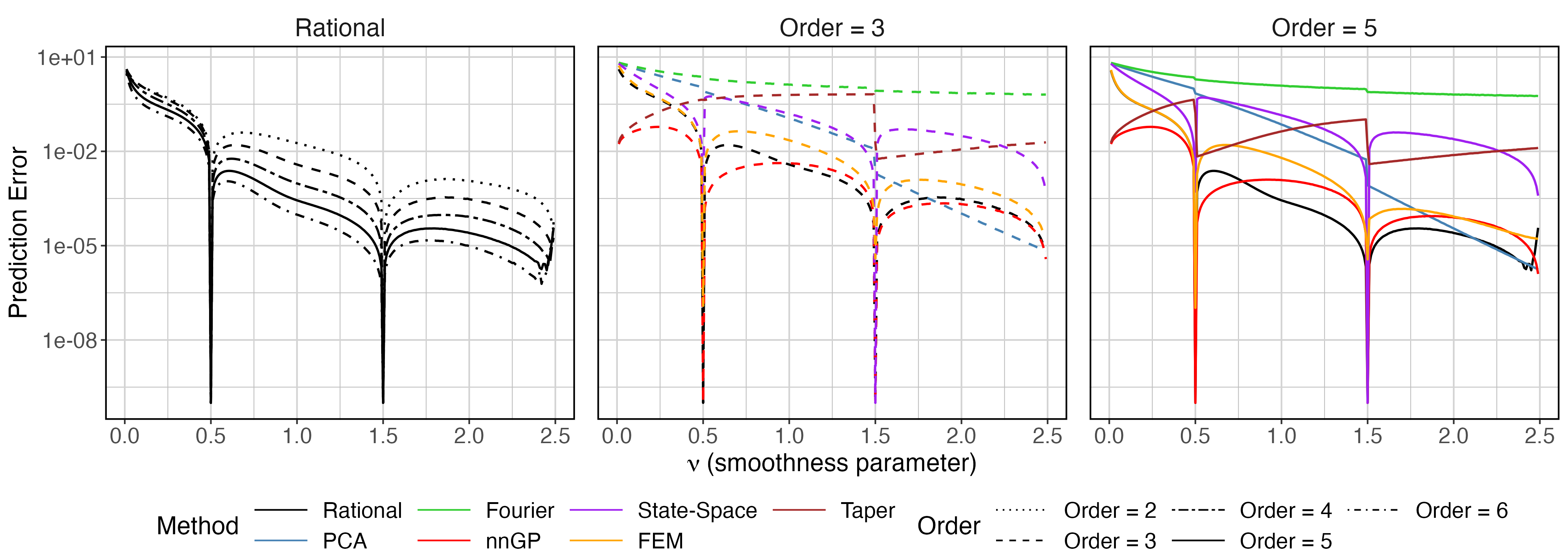
Figure 2: Prediction errors measured in mean square difference on interval $I=[0,50]$ for $\rho=2$, different values of $\nu$ and different orders of approximation.

The prediction errors shown in Figure 2 further demonstrate the advantages of the rational approximation method over the other approaches. As the approximation order $m$ increases, the mean squared error decreases consistently and rapidly to zero. For $m=3$ we can see that nnGP outperforms the rational method, by a small margin, for $\nu<1$ and the two methods have similar performance for $\nu\geq 1$. For $\nu<0.5$, the rational and FEM methods overlap. Moving to $m=5$, we can see that nnGP outperforms the rational method for small values of the smoothness parameter $\nu$, but the rational method outperforms nnGP for $\nu>0.8$. In this case, there is also an overlap between FEM and rational methods for $\nu<0.5$. It is noteworthy that the quality of the rational approximation we have available deteriorates as $\nu$ approaches zero, which suggests us that it might be possible to improve the approximation for $\nu<0.5$ by obtaining better coefficients for rational approximations in such cases. Finally, FEM provides very good accuracy, comparable to the rational and nnGP methods, whereas PCA provides the best results for large values of $\nu$, however, we recall that for one to be able to use PCA with this cost, the eigenvectors must be known.

4.4 Process approximation

As can be seen in the previous section, no alternative method is close to the proposed method in terms of accuracy of the covariance approximation. The only methods that are close to the proposed method in terms of prediction accuracy are the nnGP and FEM methods. One important difference of the nnGP method is that the approximation is strongly dependent on the support points, which typically is chosen as the observation locations in applications (Datta et al., 2016). In this section, we illustrate that this results in a poor approximation of the stochastic process, even though the approximation of the finite dimensional distribution at the support points is accurate. To this end, we consider the task of computing a joint confidence band for the latent process. Specifically, we assume that we have data ${\boldsymbol{\mathrm{y}}}=[y_{1},y_{2},\dotsc,y_{n}]$ generated as $y_{i}|u(\cdot)\sim\mathcal{N}(u(t_{i}),\sigma_{e}^{2}).$ where $t_{i}$ are $250$ locations sampled uniformly at random in the interval $(0,10)$, and $u$ is a centered Gaussian process with the Matérn covariance (1). Based on these observations, we perform prediction to $n$ evenly spaced locations in the interval, and we use the excursions package (Bolin & Lindgren, 2018) to compute the upper and lower bounds, $c_{l}(s)$ and $c_{u}(s)$, of a joint prediction interval so that

$$P(c_{l}(s)<u(s)<c_{u}(s)|{\boldsymbol{\mathrm{y}}},s\in\{p_{1},\ldots,p_{n}\})=0.9.$$

Then, for nnGP, FEM, and the proposed method, we compute the approximate coverage probabilities $\tilde{p}=\tilde{P}(c_{l}(s)<u(s)<c_{u}(s)|{\boldsymbol{\mathrm{y}}},s\in\{p_{1},\ldots,p_{n}\}),$ where $\tilde{P}(\cdot|\cdot)$ denote the posterior probability under the approximate model. If the process approximation is accurate, we expect that $\tilde{p}\approx 0.9$.

We choose $\nu=1$ and three values, $\rho=0.5,1$ and $2$, of the practical correlation range $\rho=\nicefrac{{\sqrt{8\nu}}}{{\kappa}}$. We perform this exercise for different values of $n$, while keeping the number of observations fixed at $250$. For each value of $n$, the order $m$ of the nnGP approximation is chosen so that the computational cost for evaluating the posterior mean at the prediction locations is the same as for the proposed method, and the support points for the nnGP approximation is kept fixed at the observation locations. For $n<1000$, we use the calibration cost from $n=1000$, as the observed cost in smaller cases primarily reflects computational overheads rather than the intrinsic complexity of the methods.

The error $|\tilde{p}-0.9|$ for the methods are shown as functions of $n$ in Figure 3. As expected, the error of the nnGP method increases quickly with $n$, whereas it remains more stable for the proposed approximation. This supports the claim that the proposed approximation is a better process approximation than the nnGP method. Further, the approximation is also better than the corresponding (calibrated) ones from the FEM method.

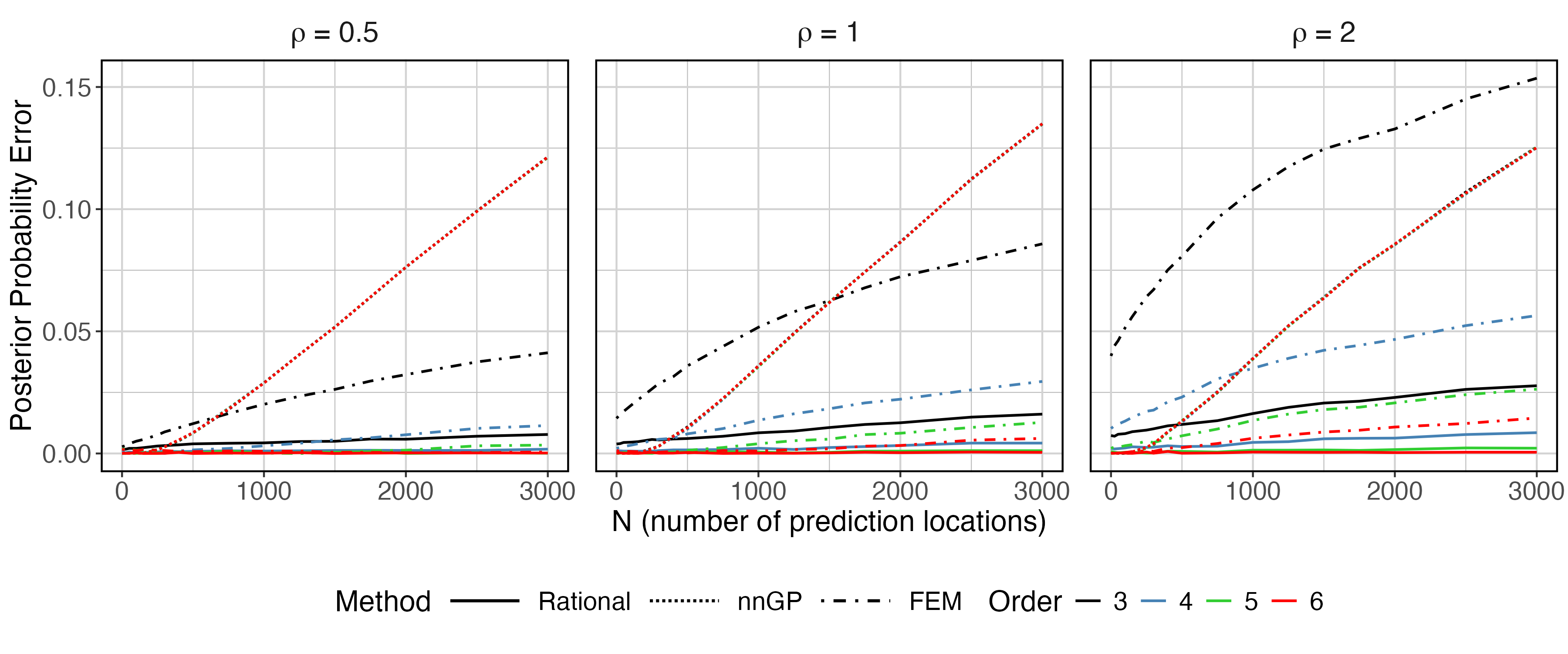
Figure 3: Absolute posterior probability errors on the interval $[0,10]$, based on $250$ observations and $N$ additional locations for $\nu=1$, $m$ from $3$ to $6$, and three different practical correlation ranges $\rho$.

5 Discussion

We have introduced a broadly applicable method for working with Gaussian processes (GPs) with Matérn covariance functions on bounded intervals, facilitating statistical inference at linear computational cost. Unlike existing approaches, which often lack theoretical guarantees for accuracy, our method achieves exponentially fast convergence of the covariance approximation. This guarantees both computational efficiency and high accuracy. Furthermore, the method yields a Markov representation of the approximated process, which simplifies its integration into general-purpose software for statistical inference.

Our experimental results demonstrate that the proposed method outperforms state-of-the-art alternatives, offering significant improvements in accuracy. The method has been implemented in the rSPDE package, which is compatible with popular tools such as R-INLA (Lindgren & Rue, 2015) and inlabru (Bachl et al., 2019), facilitating seamless integration into Bayesian hierarchical models. Further, all codes and a Shiny application can be found at https://github.com/vpnsctl/MarkovApproxMatern/.

The Shiny application also contains further comparisons for other choices of the number of prediction locations $n$, the number of observation locations $n_{obs}$, and for different practical correlation ranges of the true process. However, the general conclusions for these different choices align closely with those presented above. The main difference is that, for prediction tasks with a very small practical correlation range and an equal number of prediction and observation locations, nnGP tends to outperform all other methods, including the rational approximation. This scenario is particularly favorable for nnGP, as all locations coincide with support points. Additionally, when the number of prediction locations exceeds the number of observation locations, the rational approximation outperforms all methods, except for $\nu>1.5$, where nnGP achieves the best performance in prediction tasks.

The two most competitive methods besides the proposed method were nnGP and FEM. The nnGP model provides accurate predictions, particularly for lower values of the smoothness parameter $\nu$, as illustrated in Figure 2. However, it falls short in terms of process approximation. Specifically, the covariance errors associated with nnGP are significantly larger than those from the rational approximation method, as shown in Figure 1. Additionally, the probability approximations deteriorate markedly when observations are not contained in the support points, evidenced by Figure 3. This limitation suggests that while nnGP may provide good results in contexts focused on prediction, such as those commonly found in machine learning, it is less competitive in broader statistical applications which require accurate process approximations. The main advantage of the proposed method compared to the FEM method is a generally higher accuracy and stability, and the fact that no mesh needs to be chosen.

An exciting direction for future work involves extending our method to more general domains. As mentioned in Section 2, the method can also be derived through a rational approximation of the covariance operator of the process. More precisely, consider a Gaussian process $u$ on a domain $\mathcal{D}$ defined as the solution to

$$L^{\beta}(\tau u)=\mathcal{W},\quad\text{on }\mathcal{D},$$ (12)

where $\mathcal{W}$ is Gaussian white noise on $\mathcal{D}$, $\beta>0$ is a real number, and $L$ is a densely defined self-adjoint operator on $L_{2}(\mathcal{D})$, so that the covariance operator of $u$ is given by $L^{-2\beta}$. For example, if we have $L=(\kappa^{2}-\Delta)$ on $\mathbb{R}$, we obtain a Gaussian process with a stationary Matérn covariance function (Whittle, 1963). Following the approach in Bolin et al. (2024b), one can approximate the covariance operator as

$$L^{-2\beta}\approx L^{-\lfloor 2\beta\rfloor}\left(\sum_{i=1}^{m}r_{i}(L-p_{i}I)^{-1}+kI\right),$$ (13)

where $\{r_{i}\}_{i=1}^{m}$, $\{p_{i}\}_{i=1}^{m}$, and $k$ are real numbers, and $I:L_{2}(\mathcal{D})\to L_{2}(\mathcal{D})$ is the identity operator. If $p_{i}\leq 0$, $r_{i}>0$, and $k>0$ for all $i=1,\dots,m$, and suitable conditions on $L$ hold, this approximation expresses $L^{-2\beta}$ as a linear combination of covariance operators. We will refer to this approach as the covariance-based approach.

By computing the finite-dimensional distributions corresponding to the operators $L^{-\lfloor 2\beta\rfloor}$ and $L^{-\lfloor 2\beta\rfloor}(L-p_{i}I)^{-1}$ for $i=1,\dots,m$, we can approximate the finite-dimensional distributions of $L^{-2\beta}$ and thus the solution to (12). Assume further that these covariance operators are induced by covariance functions. Let $\varrho_{\beta}(\cdot,\cdot)$ denote the covariance function associated with $L^{-2\beta}$, $\widehat{\varrho}_{\beta}(\cdot,\cdot)$ the covariance function corresponding to $kL^{-\lfloor 2\beta\rfloor}$, and $\widehat{\varrho}_{\beta,i}(\cdot,\cdot)$ the covariance function associated with $r_{i}L^{-\lfloor 2\beta\rfloor}(L-p_{i}I)^{-1}$ for $i=1,\dots,m$. Then, (13) implies that

$$\varrho_{\beta}(x,y)\approx\widehat{\varrho}_{\beta}(x,y)+\sum_{i=1}^{m}\widehat{\varrho}_{\beta,i}(x,y),\quad x,y\in\mathcal{D},$$ (14)

which corresponds exactly to the expression in Proposition 2.1, demonstrating the equivalence between the spectral and covariance-based approaches.

It is important to note, however, that both approaches—the covariance-based and the spectral approach—yield approximations that do not converge to the true covariance operator when $\mathcal{D}=\mathbb{R}^{d}$ for $d\geq 1$. Nonetheless, one can instead consider compact domains, $\mathcal{D}$, where convergence of the approximation can generally be established.

This formulation offers a pathway for extending our method to more complex (compact) domains. For instance, starting with $L=(\kappa^{2}-\Delta)$ on a circle, one can define rational approximations for periodic Matérn fields. More generally, the approach can be adapted to network-like domains, following recent developments in Gaussian Whittle–Matérn fields on metric graphs (Bolin et al., 2023, 2024a). These extensions, including their theoretical and computational aspects, will be explored in future work. Finally, if $\mathcal{D}$ is a $d$-dimensional manifold (which also includes compact subsets of $\mathbb{R}^{d}$), where $d\geq 2$, this approach is not expected to provide sparse approximations unless $\mathcal{D}$ is a Cartesian product of intervals, and $L$ is a separable differential operator, that is, $L=\sum_{i=1}^{d}L_{i}$, where $L_{i}$ is a differential operator acting only on $x_{i}$, where $x=(x_{1},\ldots,x_{d})\in\mathcal{D}$. This implies that, while the approximation may still be applicable for manifolds of dimension greater than one, it is generally not practical unless the model is separable. Such separable models, which have been explored in previous work (see, e.g., Chen et al. (2022)), are rarely suitable for modeling spatial data.

Appendix A LDL Algorithm and proof of Proposition 3.4

In this section, we explain how to construct the matrices ${\boldsymbol{\mathrm{L}}}_{i}$ and ${\boldsymbol{\mathrm{D}}}_{i}$ of Proposition 3.4. To simplify the notation, let $p$ denote the size of the vector ${\boldsymbol{\mathrm{u}}}_{i,j}$ (which is either $\max(\lfloor\alpha\rfloor,1)$ if $i=0$ or $\lceil\alpha\rceil$ if $i>0$). Introduce the matrices ${\boldsymbol{\mathrm{B}}}^{1}={\boldsymbol{\mathrm{L}}}_{1,1}$ and ${\boldsymbol{\mathrm{B}}}^{k}=[{\boldsymbol{\mathrm{L}}}_{k,k-1}\,{\boldsymbol{\mathrm{L}}}_{k,k}],k>1,$ corresponding to the part of ${\boldsymbol{\mathrm{L}}}_{i}$ that is related to the $k$th location. Similarly, let ${\boldsymbol{\mathrm{F}}}^{k}$ denote the diagonal matrix corresponding to the part of ${\boldsymbol{\mathrm{D}}}^{-1}$ that is related to the $k$th location. That is, ${\boldsymbol{\mathrm{D}}}=\text{diag}({\boldsymbol{\mathrm{F}}}^{1},\ldots,{\boldsymbol{\mathrm{F}}}^{n})^{-1}.$ These are low-dimensional matrices with a dimension $2p\times p$ and $p\times p$, respectively. Further, introduce the covariance matrices ${\boldsymbol{\mathrm{\Sigma}}}^{1}={\boldsymbol{\mathrm{r}}}_{i}(t_{1},t_{1})$ and

$${\boldsymbol{\mathrm{\Sigma}}}^{k}=\begin{bmatrix}{\boldsymbol{\mathrm{r}}}_{i}(t_{1},t_{1})&{\boldsymbol{\mathrm{r}}}_{i}(t_{1},t_{2})\\ {\boldsymbol{\mathrm{r}}}_{i}(t_{2},t_{1})&{\boldsymbol{\mathrm{r}}}_{i}(t_{2},t_{2})\end{bmatrix},\quad k=2,\ldots,n,$$

and for an $n\times n$ matrix ${\boldsymbol{\mathrm{M}}}$, let ${\boldsymbol{\mathrm{M}}}_{a:b,c:d}$, for natural numbers $a\leq b\leq n$ and $c\leq d\leq n$ denote the submatrix obtained by extracting rows $a,\ldots,b$ and columns $c,\ldots,d$ from ${\boldsymbol{\mathrm{M}}}$.

We are now ready to construct the elements in the matrices. We set ${\boldsymbol{\mathrm{F}}}^{1}_{1,1}=1/{\boldsymbol{\mathrm{\Sigma}}}^{1}_{1,1}$ and

$${\boldsymbol{\mathrm{F}}}^{1}_{j,j} ={\boldsymbol{\mathrm{\Sigma}}}^{1}_{j,j}-{\boldsymbol{\mathrm{\Sigma}}}^{1}_{j,1:(j-1)}({\boldsymbol{\mathrm{\Sigma}}}^{1}_{1:(j-1),1:(j-1)})^{-1}{\boldsymbol{\mathrm{\Sigma}}}^{1}_{1:(j-1),j}, j=2,\ldots,p$$

$${\boldsymbol{\mathrm{F}}}^{k}_{j,j} ={\boldsymbol{\mathrm{\Sigma}}}^{k}_{p+j,p+j}-{\boldsymbol{\mathrm{\Sigma}}}^{k}_{p+j,1:(p+j-1)}({\boldsymbol{\mathrm{\Sigma}}}^{k}_{1:(p+j-1),1:(p+j-1)})^{-1}{\boldsymbol{\mathrm{\Sigma}}}^{k}_{1:(p+j-1),j}, j=1,\ldots,p,k>1.$$

Further, we set ${\boldsymbol{\mathrm{B}}}^{1}_{j,j}=1$ and ${\boldsymbol{\mathrm{B}}}^{1}_{j,j+i}=0$ for $i>0$ and

$${\boldsymbol{\mathrm{B}}}^{1}_{j,1:(j-1)}=-{\boldsymbol{\mathrm{\Sigma}}}^{1}_{j,1:(j-1)}({\boldsymbol{\mathrm{\Sigma}}}^{1}_{1:(j-1),1:(j-1)})^{-1},\quad i=2,\ldots,p.$$

Finally, we set ${\boldsymbol{\mathrm{B}}}^{k}_{j,p+j}=1$ and ${\boldsymbol{\mathrm{B}}}^{k}_{j,p+j+i}=0$ for $i>0$ and

$${\boldsymbol{\mathrm{B}}}^{k}_{j,1:(j-1)}=-{\boldsymbol{\mathrm{\Sigma}}}^{k}_{j,1:(p+j-1)}({\boldsymbol{\mathrm{\Sigma}}}^{1}_{1:(p+j-1),1:(p+j-1)})^{-1},\quad i=1,\ldots,p,k>1.$$

These expressions follow directly from using the fact that ${\boldsymbol{\mathrm{u}}}_{i}$ is a first order Markov process and then writing the joint density of ${\boldsymbol{\mathrm{u}}}_{i}$ as

$$\pi({\boldsymbol{\mathrm{u}}}_{i})=\pi({\boldsymbol{\mathrm{u}}}_{i,1})\prod_{k=w}^{n}\pi({\boldsymbol{\mathrm{u}}}_{i,k}|{\boldsymbol{\mathrm{u}}}_{i,k-1}).$$

After this, standard results for conditional Gaussian densities give the expressions above (see, for example Datta et al., 2016). To compute the elements in each block, we need to perform $p$ solves of matrices of size $p,p+1,\ldots,2p$, the total cost of this is $\mathcal{O}(p^{4})$ and since we have $n$ blocks, the total cost is thus $\mathcal{O}(np^{4})$.

Appendix B Collected proofs

We start with a simple technical lemma needed for the proof of Theorem 2.2.

Lemma B.1.

Let $h:\mathbb{R}\to\mathbb{R}$ be a measurable function. Then, the following inequality holds:

$$\int_{a}^{b}\int_{a}^{b}h(x-y)^{2}dx\,dy\leq(b-a)\int_{a-b}^{b-a}h(x)^{2}dx,$$

where $a,b\in\mathbb{R},a<b$.

Proof B.2.

We have, by the change of variables $u=x-y$, that

$$\int_{a}^{b}\int_{a}^{b}h(x-y)^{2}dx\,dy =\int_{a}^{b}\int_{a-y}^{b-y}h(u)^{2}du\,dy\leq\int_{a}^{b}\int_{a-b}^{b-a}h(u)^{2}du\,dy=(b-a)\int_{a-b}^{b-a}h(u)^{2}du,$$

where we used the fact that $a\leq y\leq b$.

Proof B.3 (of Theorem 2.2).

Our idea is to use the exponential convergence of the best rational approximation with respect to the $L_{\infty}$ norm. To such an end, Stahl (2003, Theorem 1), gives us that for every $\alpha\in(0,1)$, there exist polynomials of degree $m$, $p_{m}(\cdot)$ and $q_{m}(\cdot)$ such that the following exponential bound holds:

$$\sup_{x\in[0,1]}\left|x^{\alpha}-\frac{p_{m}(x)}{q_{m}(x)}\right|\leq Ce^{-2\pi\sqrt{\alpha m}},$$ (15)

where $C>0$ is a constant that only depends on $\alpha$. Now, let $g(w)=(1+\kappa^{-2}w^{2})^{-1}$ and observe that for every $w\in\mathbb{R}$, we have $g(w)\in[0,1]$. Further, let $\alpha=\nu+0.5$ and $f^{\alpha}(\cdot)$ be the spectral density of a stationary Gaussian process with a Matérn covariance function (1). Then, $f^{\alpha}=\kappa^{-2\alpha}(g(w))^{\alpha}$ and for any $\alpha>1/2$ we have that

$$\sup_{w\in\mathbb{R}}\left|f^{\alpha}(w)-f_{m}^{\alpha}(w)\right| =\kappa^{-2\alpha}\sup_{w\in\mathbb{R}}\left|(g(w))^{\alpha}-g(w)^{\lfloor\alpha\rfloor}\frac{p_{m}(g(w))}{q_{m}(g(w))}\right|=\kappa^{-2\alpha}\sup_{x\in[0,1]}\left|x^{\alpha}-x^{\lfloor\alpha\rfloor}\frac{p_{m}(x)}{q_{m}(x)}\right|$$

$$=\kappa^{-2\alpha}\sup_{x\in[0,1]}x^{\lfloor\alpha\rfloor}\left|x^{\{\alpha\}}-\frac{p_{m}(x)}{q_{m}(x)}\right|\leq Ce^{-2\pi\sqrt{\alpha m}},$$

where we used (15) and the fact that $0\leq x\leq 1$. Now, let $I=[a,b]\subset\mathbb{R}$ be an interval in $\mathbb{R}$ and $1_{I}:\mathbb{R}\rightarrow\mathbb{R}$ denote the indicator function such that $1_{I}(x)=1$ if $x\in I$ and $1_{I}(x)=0$ otherwise. We then have by Plancherel’s theorem (e.g. McLean, 2000, Corollary 3.13), the convolution theorem (e.g. McLean, 2000, p.73), Lemma B.1, and the bound above that

$$\|r_{m}^{\alpha}-r^{\alpha}\|_{L_{2}(I\times I)}^{2} \leq(b-a)\|\varrho_{m}^{\alpha}-\varrho^{\alpha}\|_{L_{2}(a-b,b-a)}^{2}=(b-a)\|(\varrho_{m}^{\alpha}-\varrho^{\alpha})1_{[a-b,b-a)]}\|_{L_{2}(\mathbb{R})}^{2}$$

$$=(b-a)\left\|(f_{m}^{\alpha}-f^{\alpha})\ast 2(b-a)\frac{\sin((b-a)w)}{(b-a)w}\right\|_{L_{2}(\mathbb{R})}^{2}$$

$$\leq(b-a)\sup_{w\in\mathbb{R}}\left(f^{\{\alpha\}}(w)-\frac{p_{m}(w)}{q_{m}(w)}\right)^{2}\left\|2(b-a)\frac{\sin((b-a)w)}{(b-a)w}\right\|_{L_{2}(\mathbb{R})}^{2}$$

$$\leq(b-a)\widehat{C}e^{-2\pi\sqrt{\{\alpha\}m}},$$

where the constant $\widehat{C}$ only depends on $\alpha,\kappa$ and $\sigma$, and $\ast$ denotes the convolution. This proves (5).

Now, for the $L_{\infty}(I\times I)$ estimate. Recall the notation from the first part of the proof. Also, recall the definition of the Sobolev space $H^{s}(\mathbb{R})$ for $s\geq 0$ (see, e.g. McLean, 2000, p.75-76). Then, for $s>\nicefrac{{1}}{{2}}$, we have by definition of the Sobolev norm that

$$\|\varrho^{\alpha}-\varrho_{m}^{\alpha}\|_{H^{s}(\mathbb{R})} =\|(1+w^{2})^{\nicefrac{{s}}{{2}}}(f^{\alpha}-f_{m}^{\alpha})\|_{L_{2}(\mathbb{R})}\leq\sup_{w\in\mathbb{R}}\left|f^{\{\alpha\}}(w)-\frac{p_{m}(w)}{q_{m}(w)}\right|\|f^{\lfloor\alpha\rfloor}(1+w^{2})^{\nicefrac{{s}}{{2}}}\|_{L_{2}(\mathbb{R})}$$

$$\leq\widetilde{C}e^{-2\pi\sqrt{\{\alpha\}m}}\|(1+w^{2})^{s/2-\lfloor\alpha\rfloor}\|_{L_{2}(\mathbb{R})},$$

where $\widetilde{C}$ is a constant that only depends on $\kappa,\sigma$ and $\alpha$. Now, observe that since $\alpha>1$, we have that $\lfloor\alpha\rfloor\geq 1$. Further, note that $\|(1+w^{2})^{s/2-\lfloor\alpha\rfloor}\|_{L_{2}(\mathbb{R})}<\infty$ if, and only if, $2\lfloor\alpha\rfloor-s>\nicefrac{{1}}{{2}}$. In particular, since $\lfloor\alpha\rfloor\geq 1$ we can find $s>\nicefrac{{1}}{{2}}$ such that $\|(1+w^{2})^{s/2-\lfloor\alpha\rfloor}\|_{L_{2}(\mathbb{R})}<\infty$. Therefore, if $\alpha>1$, we can find $s>\nicefrac{{1}}{{2}}$ such that $\|\varrho^{\alpha}-\varrho_{m}^{\alpha}\|_{H^{s}(\mathbb{R})}\leq\breve{C}e^{-2\pi\sqrt{\{\alpha\}m}},$ where the constant $\breve{C}$ depends on $s>\nicefrac{{1}}{{2}}$, $\kappa$, $\sigma$ and $\alpha$. Now, from Sobolev embedding, see, e.g., (McLean, 2000, Theorem 3.26), if $s>\nicefrac{{1}}{{2}}$, we have that there exists $C_{sob}>0$, depending only on $s$, such that for every $x\in\mathbb{R}$, $|\varrho^{\alpha}(x)-\varrho_{m}^{\alpha}(x)|\leq C_{sob}\|\varrho^{\alpha}-\varrho_{m}^{\alpha}\|_{H^{s}(\mathbb{R})},$ so that

$$\sup_{x\in\mathbb{R}}|\varrho^{\alpha}(x)-\varrho_{m}^{\alpha}(x)|\leq C_{sob}\|\varrho^{\alpha}-\varrho_{m}^{\alpha}\|_{H^{s}(\mathbb{R})}\leq C_{sob}\breve{C}e^{-2\pi\sqrt{\{\alpha\}m}}.$$

Therefore, $\|r_{m}^{\alpha}-r^{\alpha}\|_{L_{\infty}(I\times I)}\leq\sup_{x\in\mathbb{R}}|\varrho^{\alpha}(x)-\varrho_{m}^{\alpha}(x)|\leq C_{sob}\breve{C}e^{-2\pi\sqrt{\{\alpha\}m}}.$ This proves (6).

Proof B.4 (of Proposition 2.1).

Note that

$$\frac{1}{(\kappa^{2}p)^{k}(\kappa^{2}(1-p)+w^{2})}-\sum_{j=1}^{k}\frac{1}{(\kappa^{2}p)^{k+1-j}(\kappa^{2}+w^{2})^{j}}$$

$$\quad=\frac{1}{(\kappa^{2}p)^{k}(\kappa^{2}(1-p)+w^{2})}-\frac{1}{(\kappa^{2}p)^{k+1}}\sum_{j=1}^{k}\left(\frac{\kappa^{2}p}{\kappa^{2}+w^{2}}\right)^{j}=\frac{1}{(\kappa^{2}+w^{2})^{k}(\kappa^{2}(1-p)+w^{2})},$$

where we used the closed-form expression of the geometric sum to arrive at the final identity. Based on this, we can rewrite the spectral density (3) as

$$f_{m}^{\alpha}(w)= A\sigma^{2}\kappa^{-2\alpha}\bigg{[}\frac{k\kappa^{2\lfloor\alpha\rfloor}}{(\kappa^{2}+w^{2})^{\lfloor\alpha\rfloor}}$$ (16)

$$~{}+\sum_{i=1}^{m}r_{i}\kappa^{2\lfloor\alpha\rfloor+2}\bigg{(}\sum_{j=1}^{\lfloor\alpha\rfloor}\frac{1}{(\kappa^{2}p)^{\lfloor\alpha\rfloor}(\kappa^{2}(1-p_{i})+w^{2})}-\frac{1}{(\kappa^{2}p)^{\lfloor\alpha\rfloor+1-j}(\kappa^{2}+w^{2})^{j}}\bigg{)}\bigg{]}.$$

Finally, the explicit expression for the covariance function (4) thus directly follows by taking the inverse Fourier transform of spectral density (16) and using the linearity of the inverse Fourier transform.

Proof B.5 (of Proposition 3.1).

We begin by recalling that if $v(\cdot)$ is a stationary Gaussian process on $\mathbb{R}$ with spectral density $h$, then by (Pitt, 1971, Theorem 10.1), the process $v$ will be a Markov process of order $p$, $p\in\mathbb{N}$, on $\mathbb{R}$, if, and only if, the spectral density of $v$, namely $h$, is a reciprocal of a polynomial of degree $2p$.

The spectral density of the process $u_{0}$ is $f_{m,0}^{\alpha}$ and the spectral density of $u_{i}$, $i=1,\ldots,m$, is $f_{m,i}^{\alpha}$, where $f_{m,0}^{\alpha}$ and $f_{m,i}^{\alpha}$ were defined in (3). Moreover, observe that $f_{m,0}^{\alpha}$ is a reciprocal of a polynomial with degree $2\lfloor\alpha\rfloor$, and $f_{m,i}^{\alpha}$, $i=1,\ldots,m$, are reciprocals of polynomials of degree $2(\lfloor\alpha\rfloor+1)$, thus $u_{0}$ is a markov process of order $\lfloor\alpha\rfloor$ and $u_{j},j=1,\ldots,m$ are Markov processes of order $\lfloor\alpha\rfloor+1$. Now, it is well-known, see Whittle (1963) and (Lindgren, 2012, Theorem 4.7 and 4.8), that $u_{0}$ also solves

$$\begin{cases}k(\kappa+\partial_{x})(\kappa^{2}-\Delta)^{\frac{\lfloor\alpha\rfloor-1}{2}}u_{0}=\mathcal{W}&\text{when}~{}\lfloor\alpha\rfloor~{}\text{is odd},\\ k(\kappa^{2}-\Delta)^{\frac{\lfloor\alpha\rfloor}{2}}u_{0}=\mathcal{W}&\text{when}~{}\lfloor\alpha\rfloor~{}\text{is even},\end{cases}$$

in the sense that the solution to the above equation has the same covariance function as $u_{0}$. Similarly, we also have that $u_{i}$ solves

$$\begin{cases}r_{i}(\kappa\sqrt{1-p_{i}}+\partial_{x})(\kappa+\partial_{x})(\kappa^{2}-\Delta)^{\frac{\lfloor\alpha\rfloor-1}{2}}u_{i}=\mathcal{W},&\text{when}~{}\lfloor\alpha\rfloor~{}\text{is odd},\\ r_{i}(\kappa\sqrt{1-p_{i}}+\partial_{x})(\kappa^{2}-\Delta)^{\nicefrac{{\lfloor\alpha\rfloor}}{{2}}}u_{i}=\mathcal{W},&\text{when}~{}\lfloor\alpha\rfloor~{}\text{is even},\end{cases}$$

on interval $I$. Now, since each process is stationary, we start with the stationary distribution, i.e., ${\boldsymbol{\mathrm{u}}}_{0}=[u_{0}(0),u^{\prime}_{0}(0),\dotsc,u_{0}^{(\lfloor\alpha\rfloor)}(0)]^{\top}$ and ${\boldsymbol{\mathrm{u}}}_{i}=[u_{i}(0),u_{i}^{\prime}(0),\dotsc,u_{i}^{(\lceil\alpha\rceil)}(0)]^{\top}$, $i>0$, follow the stationary distribution, and thus, the restrictions of these processes from $\mathbb{R}$ to interval $I$ will also be Markov. Therefore, the tridiagonal structure of the precision matrix follows from the fact that if we consider the open set $O_{j}=(j-1,j+1)$, $j\geq 2$, $j\in\mathbb{N}$, contained in interval $I$, then, in view of the Markov property we have that for each $i=0,\dotsc,m$, ${\boldsymbol{\mathrm{u}}}_{i,j}\perp{\boldsymbol{\mathrm{u}}}_{i,k}|{\boldsymbol{\mathrm{u}}}_{i,j-1},{\boldsymbol{\mathrm{u}}}_{i,j+1}$ for $k\in I\backslash\{j-1,j,j+1\}$, where ${\boldsymbol{\mathrm{u}}}_{0,j}=(u_{0}(w_{j}),\dotsc,u_{0}^{(\lfloor\alpha\rfloor)}(w_{j}))$ and ${\boldsymbol{\mathrm{u}}}_{i,j}=(u_{i}(w_{j}),\dotsc,u_{i}^{(\lceil\alpha\rceil)}(w_{j}))$, $i=1,2,\dotsc,m$, $w_{j}\in O_{j}$. Finally, by using this conditional independences and standard techniques (see, for example, the computations of Rue & Held (2005) for conditional autoregressive models), we obtain the expressions for the local precision matrices ${\boldsymbol{\mathrm{Q}}}_{i,j}$, $i,j=1,\ldots,n$.

Proof B.6 (of Proposition 3.3.).

First, recall that $N=n\left(m\lceil\alpha\rceil+\max(\lfloor\alpha\rfloor,1)\right).$ According to Algorithm 2.9 in Rue & Held (2005), the computational cost of factorizing an $n\times n$ band matrix with bandwidth $p$ is $n(p^{2}+3p)$, and solving a linear system via back-substitution requires $2np$ floating-point operations. Since ${\boldsymbol{\mathrm{Q}}}$ is an $N\times N$ matrix with bandwidth $2\lfloor\alpha\rfloor+1$, the total number of floating-point operations required for the Cholesky factorization is $n\left(m\lceil\alpha\rceil+\max(\lfloor\alpha\rfloor,1)\right)\left((2\lfloor\alpha\rfloor+1)^{2}+3(2\lfloor\alpha\rfloor+1)\right).$ Similarly, the floating-point operations required for solving the linear system are $2n\left(m\lceil\alpha\rceil+\max(\lfloor\alpha\rfloor,1)\right)(2\lfloor\alpha\rfloor+1).$

Proof B.7 (of Proposition 3.5).

By reordering $\bar{{\boldsymbol{\mathrm{U}}}}$ by location, i.e.

$$\bar{{\boldsymbol{\mathrm{U}}}}=[{\boldsymbol{\mathrm{u}}}_{0}(t_{1}),{\boldsymbol{\mathrm{u}}}_{1}(t_{1}),\ldots,{\boldsymbol{\mathrm{u}}}_{m}(t_{1}),{\boldsymbol{\mathrm{u}}}_{0}(t_{2}),{\boldsymbol{\mathrm{u}}}_{1}(t_{2}),\ldots]^{\top},$$

we have that ${\boldsymbol{\mathrm{Q}}}_{\bar{{\boldsymbol{\mathrm{U}}}}|{\boldsymbol{\mathrm{y}}}}$ is an $N\times N$ matrix, with bandwidth $\lceil\alpha\rceil(m+1)$. Following the same strategy as in the proof of Proposition 3.3 gives that the Cholesky factor can be computed in

$$n(m\lceil\alpha\rceil+\max(\lfloor\alpha\rfloor,1))(\lceil\alpha\rceil^{2}(m+1)^{2}+3\lceil\alpha\rceil(m+1))$$

floating point operations, and $2n(m\lceil\alpha\rceil+1)\lceil\alpha\rceil(m+1)$ floating point operations are needed for solving a linear system through back-substitution. Computing the reordering of $\bar{{\boldsymbol{\mathrm{U}}}}$ and reordering the results back can clearly be done in $\mathcal{O}(N)$ cost as the reordering is explicitly known.

References

- Bachl et al. (2019) Bachl, F. E., Lindgren, F., Borchers, D. L. & Illian, J. B. (2019). inlabru: an R package for Bayesian spatial modelling from ecological survey data. Methods in Ecology and Evolution 10, 760–766.
- Baker & Morris (1996) Baker, G. A. & Morris, P. G. (1996). Padé approximants (second ed.). Volume 59 of Encyclopedia of Mathematics and its Applications Cambridge University Press, Cambridge.
- Bolin et al. (2020) Bolin, D., Kirchner, K. & Kovács, M. (2020). Numerical solution of fractional elliptic stochastic PDEs with spatial white noise. IMA Journal of Numerical Analysis 40, 1051–1073.
- Bolin & Lindgren (2018) Bolin, D. & Lindgren, F. (2018). Calculating probabilistic excursion sets and related quantities using excursions. Journal of Statistical Software 86, 1–20.
- Bolin & Simas (2023) Bolin, D. & Simas, A. B. (2023). rSPDE: Rational Approximations of Fractional Stochastic Partial Differential Equations. R package version 2.3.3.
- Bolin et al. (2023) Bolin, D., Simas, A. B. & Wallin, J. (2023). Statistical inference for Gaussian Whittle–Matérn fields on metric graphs. arXiv preprint arXiv:2304.10372 .
- Bolin et al. (2024a) Bolin, D., Simas, A. B. & Wallin, J. (2024a). Gaussian Whittle–Matérn fields on metric graphs. Bernoulli 30, 1611–1639.
- Bolin et al. (2024b) Bolin, D., Simas, A. B. & Xiong, Z. (2024b). Covariance–based rational approximations of fractional SPDEs for computationally efficient bayesian inference. Journal of Computational and Graphical Statistics 33, 64–74.
- Chen et al. (2022) Chen, H., Ding, L. & Tuo, R. (2022). Kernel packet: An exact and scalable algorithm for Gaussian process regression with Matérn correlations. Journal of machine learning research 23, 1–32.
- Cressie & Johannesson (2008) Cressie, N. & Johannesson, G. (2008). Fixed rank kriging for very large spatial data sets. Journal of the Royal Statistical Society. Series B. Statistical Methodology 70, 209–226.
- Datta et al. (2016) Datta, A., Banerjee, S., Finley, A. O. & Gelfand, A. E. (2016). Hierarchical nearest-neighbor Gaussian process models for large geostatistical datasets. Journal of the American Statistical Association 111, 800–812.
- Furrer et al. (2006) Furrer, R., Genton, M. & Nychka, D. (2006). Covariance tapering for interpolation of large spatial datasets. Journal of Computational and Graphical Statistics 15, 502–523.
- Gramacy (2020) Gramacy, R. B. (2020). Surrogates: Gaussian process modeling, design, and optimization for the applied sciences. Chapman and Hall/CRC.
- Gramacy & Apley (2015) Gramacy, R. B. & Apley, D. W. (2015). Local Gaussian process approximation for large computer experiments. Journal of Computational and Graphical Statistics 24, 561–578.
- Hartikainen & Särkkä (2010) Hartikainen, J. & Särkkä, S. (2010). Kalman filtering and smoothing solutions to temporal Gaussian process regression models. In 2010 International Workshop on Machine Learning for Signal Processing. IEEE.
- Higdon (2002) Higdon, D. (2002). Space and space-time modeling using process convolutions. Quantitative methods for current environmental issues 3754, 37–56.
- Hofreither (2021) Hofreither, C. (2021). An algorithm for best rational approximation based on barycentric rational interpolation. Numerical Algorithms 88, 365–388.
- Hong et al. (2023) Hong, Y., Song, Y., Abdulah, S., Sun, Y., Ltaief, H., Keyes, D. E. & Genton, M. G. (2023). The third competition on spatial statistics for large datasets. Journal of Agricultural, Biological and Environmental Statistics 28, 618–635.
- Karvonen & Särkkä (2016) Karvonen, T. & Särkkä, S. (2016). Approximate state-space Gaussian processes via spectral transformation. In 2016 IEEE 26th International Workshop on Machine Learning for Signal Processing (MLSP). IEEE.
- Lindgren et al. (2022) Lindgren, F., Bolin, D. & Rue, H. (2022). The SPDE approach for Gaussian and non-Gaussian fields: 10 years and still running. Spatial Statistics , 100599.
- Lindgren & Rue (2015) Lindgren, F. & Rue, H. (2015). Bayesian spatial modelling with r-inla. J. Stat. Softw. 63.
- Lindgren et al. (2011) Lindgren, F., Rue, H. & Lindström, J. (2011). An explicit link between Gaussian fields and Gaussian Markov random fields: the stochastic partial differential equation approach. Journal of the Royal Statistical Society. Series B. Statistical Methodology 73, 423–498. With discussion and a reply by the authors.
- Lindgren (2012) Lindgren, G. (2012). Stationary stochastic processes: theory and applications. CRC Press.
- Ling (2019) Ling, Y. (2019). Superfast inference for stationary Gaussian processes in particle tracking microrheology. PhD Thesis. http://hdl.handle.net/10012/15338.
- Ling & Lysy (2022) Ling, Y. & Lysy, M. (2022). SuperGauss: Superfast Likelihood Inference for Stationary Gaussian Time Series. R package version 2.0.3.
- Matérn (1960) Matérn, B. (1960). Spatial variation. Meddelanden från statens skogsforskningsinstitut 49.
- McLean (2000) McLean, W. (2000). Strongly elliptic systems and boundary integral equations. Cambridge University Press.
- Nychka et al. (2015) Nychka, D., Bandyopadhyay, S., Hammerling, D., Lindgren, F. & Sain, S. (2015). A multiresolution Gaussian process model for the analysis of large spatial datasets. Journal of Computational and Graphical Statistics 24, 579–599.
- Padidar et al. (2021) Padidar, M., Zhu, X., Huang, L., Gardner, J. & Bindel, D. (2021). Scaling Gaussian processes with derivative information using variational inference. Advances in Neural Information Processing Systems 34, 6442–6453.
- Pitt (1971) Pitt, L. D. (1971). A Markov property for Gaussian processes with a multidimensional parameter. Archive for Rational Mechanics and Analysis 43, 367–391.
- Porcu et al. (2023) Porcu, E., Bevilacqua, M., Schaback, R. & Oates, C. J. (2023). The Matŕn model: A journey through statistics, numerical analysis and machine learning. arXiv preprint arXiv:2303.02759 .
- Rahimi & Recht (2007) Rahimi, A. & Recht, B. (2007). Random features for large-scale kernel machines. Advances in neural information processing systems 20.
- Remez (1934) Remez, E. Y. (1934). Sur la détermination des polynômes d’approximation de degré donnée. Communications of the Kharkov Mathematical Society 10, 41–63.
- Roininen et al. (2018) Roininen, L., Lasanen, S., Orispää, M. & Särkkä, S. (2018). Sparse approximations of fractional Matérn fields. Scandinavian Journal of Statistics. Theory and Applications 45, 194–216.
- Roos et al. (2021) Roos, F. D., Gessner, A. & Hennig, P. (2021). High-dimensional Gaussian process inference with derivatives. In International Conference on Machine Learning. PMLR.
- Rue & Held (2005) Rue, H. & Held, L. (2005). Gaussian Markov random fields, vol. 104 of Monographs on Statistics and Applied Probability. Chapman & Hall/CRC, Boca Raton, FL. Theory and applications.
- Rue et al. (2009) Rue, H., Martino, S. & Chopin, N. (2009). Approximate Bayesian inference for latent Gaussian models using integrated nested Laplace approximations (with discussion). Journal of the Royal Statistical Society. Series B. Statistical Methodology 71, 319–392.
- Santner et al. (2003) Santner, T. J., Williams, B. J., Notz, W. I. & Williams, B. J. (2003). The design and analysis of computer experiments, vol. 1. Springer.
- Särkkä & Hartikainen (2012) Särkkä, S. & Hartikainen, J. (2012). Infinite-dimensional Kalman filtering approach to spatio-temporal Gaussian process regression. In Artificial intelligence and statistics. PMLR.
- Särkkä et al. (2013) Särkkä, S., Solin, A. & Hartikainen, J. (2013). Spatiotemporal learning via infinite-dimensional Bayesian filtering and smoothing: A look at Gaussian process regression through Kalman filtering. IEEE Signal Processing Magazine 30, 51–61.
- Solak et al. (2002) Solak, E., Smith, R. M., Leithead, W. E., Leith, D. & Rasmussen, C. (2002). Derivative observations in Gaussian process models of dynamic systems. Advances in neural information processing systems 15.
- Srinivas et al. (2009) Srinivas, N., Krause, A., Kakade, S. M. & Seeger, M. (2009). Gaussian process optimization in the bandit setting: No regret and experimental design. arXiv preprint arXiv:0912.3995 .
- Stahl (2003) Stahl, H. R. (2003). Best uniform rational approximation of on [0, 1]. Acta mathematica 190, 241–306.
- Stein (1999) Stein, M. L. (1999). Interpolation of spatial data. Springer series in statistics. Springer New York.
- Tronarp et al. (2018) Tronarp, F., Karvonen, T. & Särkkä, S. (2018). Mixture representation of the Matérn class with applications in state space approximations and Bayesian quadrature. In 2018 IEEE 28th International Workshop on Machine Learning for Signal Processing (MLSP). IEEE.
- Vecchia (1988) Vecchia, A. V. (1988). Estimation and model identification for continuous spatial processes. Journal of the Royal Statistical Society. Series B. Methodological 50, 297–312.
- Wang (2008) Wang, L. (2008). Karhunen-Loève expansions and their applications. London School of Economics and Political Science (United Kingdom).
- Whittle (1963) Whittle, P. (1963). Stochastic processes in several dimensions. Bull. Internat. Statist. Inst. 40, 974–994.
- Wood & Chan (1994) Wood, A. T. & Chan, G. (1994). Simulation of stationary Gaussian processes in . Journal of computational and graphical statistics 3, 409–432.
- Yang et al. (2018) Yang, A., Li, C., Rana, S., Gupta, S. & Venkatesh, S. (2018). Sparse approximation for Gaussian process with derivative observations. In Australasian Joint Conference on Artificial Intelligence. Springer.