Resonances and resonance expansions
for point interactions on the half-space

Abstract.

In this paper we describe the resonances of the singular perturbation of the Laplacian on the half space $\Omega=\mathbb{R}^{3}_{+}$ given by the self-adjoint operator named $\delta$-interaction or point interaction. We will assume Dirichlet or Neumann boundary conditions on $\partial\Omega$. At variance with the well known case of $\mathbb{R}^{3}$, the resonances constitute an infinite set, here completely characterized. Moreover, we prove that resonances have an asymptotic distribution satisfying a modified Weyl law. Finally we give applications of the results to the asymptotic behavior of the abstract Wave and Schrödinger dynamics generated by the Laplacian with a point interaction on the half-space.

Keywords: Point interactions; Spectral theory; Resonances

MSC 2020: 35P25, 47A40, 81U15, 58J50

1. Introduction

Schrödinger operators $H$ on unbounded domains, besides a rich and much developed spectral theory, are characterized by the existence of resonances, i.e. poles of the meromorphic continuation in the lower complex half-plane of the resolvent $(H-z^{2})^{-1}$. Loosely speaking, resonances behave as a sort of complex eigenvalues; associated to them there are resonance functions, playing the role of eigenfunctions but only locally square integrable. The use of resonances is common in Physics and their importance is due to the fact that when $H$ is the generator of a Schrödinger or wave dynamics, they correspond to states decaying in time (at least for sufficiently long times), the slower ones (and so the more physically meaningful) being the nearest to the real axis. Among other reasons, resonances are of interest because the solution of the Wave or Schrödinger equation propagating on non-compact domains can be expressed, asymptotically for large times and for initial data localized in space, as an expansion based on resonance functions [1, 26, 21] as an alternative to the expansion based on the spectral theorem. For these and other reasons, it is desirable to have as precise information as possible about the location and properties of resonances of self-adjoint operators. While a lot of rigorous results have been accumulated along the years about general qualitative properties of resonances and their several applications in Physics, Dynamical Systems theory and Geometry (see the treatise [21] for an encyclopedic and recent account), precise and quantitative information also for specific classes of operators is however rare. In this paper we want to begin the analysis of the resonances of the class of self-adjoint singular perturbations of the Laplacian called $\delta$-interactions or point interactions and considered on domains of $\mathbb{R}^{n},\ n=2,3$. There is a huge literature on point interactions (see [2] for the bibliography until 2005, still growing). Their interest is due mostly to the fact that, in many case, they represent exactly solvable models in Quantum Mechanics and that they are suitable scaling limit of more realistic, non solvable models. However, they have been studied almost exclusively on the whole space $\mathbb{R}^{n},\ n=1,2,3$. Only a handful of papers treats the case of bounded domains (see [12]) of hyperbolic space (see the recent [20], including also point interactions on spheres) and essentially nothing is known about unbounded domains in $\mathbb{R}^{n}$. As regards resonances, the laplacian with a single point interaction in $\mathbb{R}^{n},\ n=1,2,3$ has at most a single resonance, a strong difference with standard Schrödinger operators $H=-\Delta+V$. On the contrary, $N$-point delta interactions have infinitely many resonances. This has been recognized originally in [4], and later the distribution of complex resonances has been investigated again by Albeverio and Karabash [7, 6, 5] and by Lipovský and Lotoreichik [27]. The special case of real resonances in dimension 3 is discussed in [28]. Properties of the resolvent in dimension two are instead studied in [14], but the analysis of resonances of point interactions in dimension two is still rather poor. The one dimensional case is the best known, and see in particular the recent papers [17] and [32]. We stress that the treatment of the one dimensional case is greatly simplified by the fact that the $\delta$ distribution can be considered as a form bounded perturbation of the laplacian and can be treated, formally but safely, as a standard potential. This is quite not the case in higher dimension, where the point interaction cannot be properly interpreted as a kind of Schrödinger operator "$-\Delta+\delta$".
As regards resonances, little is known when the domain considered is an unbounded subset of $\mathbb{R}^{n}$, apart from the one dimensional case, where the half-line with a delta potential and a Dirichlet boundary conditions (called Winter model in the physical literature) has received some attention ([16, 32] and references therein). Here we consider probably the simplest case of the half-space with Dirichlet or Neumann boundary conditions on the boundary, and a point interaction at a generic position $y$. The plan of the paper is the following. In Section 2 point interactions on the half-space are introduced, giving their complete definition and relevant properties. Because a rather standard construction is involved in the rigorous definition, we omit proofs of Proposition 2.1 and Proposition 2.2. We stress that these model cases do not reduce to any combinations of point interactions in $\mathbb{R}^{3}$ (see Remark 2.5 and Remark 3.8). Then, in Section 3 we obtain the explicit calculation of all the resonances of the considered models, here with full details and relevant remarks. The explicit knowledge of the set of resonances allows, in Section 4, to give results about their counting in spherical neighborhoods of given radius in the complex plane. It should be noticed that the distribution does not resembles the analogous one for smooth potentials in dimension three. This different behavior was already noticed in [27] for several point interactions in $\mathbb{R}^{3}$ and it is here confirmed for a domain not coinciding with $\mathbb{R}^{3}$. Finally, in Section 5 the expansion in resonances is deduced from the previous information, both for the wave and Schrödinger evolution. The resonance expansion for point interactions was previously considered in [1] for arrays of point interactions in $\mathbb{R}^{3}$ and in [11] where a quantized model of matter and radiation introduced in [30, 29] is studied.
We finally notice that the extension of the results obtained in the present paper to domains more general than the half-space, or the analysis of the two dimensional case, seem to be interesting tasks and they will be the object of future research.

2. Preliminaries: Point Interaction on the half-space

In this section we introduce the definition of the Laplacian with a point interaction in the half-space. A definition of this kind of operators suitable for rather general domains in $\mathbb{R}^{3}$ could be obtained by means of the theory of self-adjoint extensions of symmetric operators, but in the special case here studied a direct definition will suffice.
The half-space is $\mathbb{R}_{+}^{3}=\Set{x=(x_{1},x_{2},x_{3})\in\mathbb{R}^{3}}{x_{3}>0}$ and its boundary is $\partial\mathbb{R}^{3}_{+}=\left\{x=(x_{1},x_{2},x_{3})\in\mathbb{R}^{3}\ |\ x_{3}=0\right\}$.
We denote with $G_{z,y}^{0}$ the Green’s function centered at $y\in\mathbb{R}^{3}$ for the operator $-\Delta-z^{2}$ on the whole space

(2.1) $$G_{z,y}^{0}(x)=\frac{e^{iz\left\lvert x-y\right\rvert}}{4\pi\left\lvert x-y\right\rvert}\ ,\quad\quad\quad\operatorname{Im}z>0\ .$$

Notice that $\operatorname{Im}z>0$ implies $z^{2}\in\mathbb{C}\setminus[0,+\infty)$, the resolvent set of the free laplacian on $\mathbb{R}^{3}$.
The Green function centered at $y\in\mathbb{R}^{3}_{+}$ of the operator $-\Delta-z^{2}$ on the half-space $\mathbb{R}_{+}^{3}$ with Dirichlet or Neumann boundary conditions is given respectively by

(2.2) $$G_{z,y}^{\text{D}}=G_{z,y}^{0}-h_{z,y}^{\textup{D}}\quad\textup{or}\quad G_{z,y}^{\textup{N}}=G_{z,y}^{0}-h_{z,y}^{\textup{N}},$$

where $h_{z,y}^{\textup{D}}$ and $h_{z,y}^{\textup{N}}$ solve in the classical sense respectively the following boundary value problems

(2.3) $$\begin{cases}(-\Delta-z^{2})h_{z,y}^{\textup{D}}=0\quad&\textup{in}\ \mathbb{R}_{+}^{3}\\ h_{z,y}^{\textup{D}}=G_{z,y}^{0}\quad&\textup{in}\ \partial\mathbb{R}^{3}_{+}\end{cases}\quad\text{or}\quad\begin{cases}(-\Delta-z^{2})h_{z,y}^{\textup{N}}=0\quad&\textup{in}\,\mathbb{R}_{+}^{3}\\ \frac{\partial h_{z,y}^{\textup{N}}}{\partial x_{3}}=\frac{\partial G_{z,y}^{0}}{\partial x_{3}}\quad&\textup{in}\,\partial\mathbb{R}^{3}_{+}\end{cases}.$$

By a simple symmetry argument it follows the well-known fact that

(2.4) $$h_{z,y}^{\textup{D}}(x)=\frac{e^{iz\left\lvert x-\overline{y}\right\rvert}}{4\pi\left\lvert x-\overline{y}\right\rvert}\quad\textup{and}\quad h_{z,y}^{\textup{N}}(x)=-\frac{e^{iz\left\lvert x-\overline{y}\right\rvert}}{4\pi\left\lvert x-\overline{y}\right\rvert},\ \ \ \ \ \ \operatorname{Im}z>0$$

where $\overline{y}=(y_{1},y_{2},-y_{3})$ denotes the reflected of the point $y$ with respect to the plane $x_{3}=0$.
Moreover we will denote with $-\Delta^{\textup{D}}$ and $-\Delta^{\textup{N}}$ the free Laplacian on $\mathbb{R}_{+}^{3}$ with Dirichlet and Neumann boundary conditions respectively on $\partial\mathbb{R}^{3}_{+}$, considered as self-adjoint operators on $L^{2}(\mathbb{R}^{3}_{+})$. These operators have the respective domains

$$D(-\Delta^{\textup{D}}) =H^{2}(\mathbb{R}^{3}_{+})\cap H^{1}_{0}(\mathbb{R}^{3}_{+})$$

$$D(-\Delta^{\textup{N}}) =H^{2}(\mathbb{R}^{3}_{+})\ .$$

The resolvent set of $-\Delta^{\textup{D}}$ and $-\Delta^{\textup{N}}$ is still $\mathbb{C}\setminus[0,+\infty)$.
Let us fix an arbitrary $y\in\mathbb{R}_{+}^{3}$, where the singular interaction is placed. A straightforward calculation allows to check that the symmetric non self-adjoint operators

(2.5) $$-\Delta^{\textup{D}} \ \ \text{with domain}\ \ \mathring{D}(-\Delta^{\textup{D}})=\left\{\psi\in L^{2}(\mathbb{R}^{3}_{+})\ \text{s.t.}\ \ \psi\in D(-\Delta^{\textup{D}}),\ \psi(y)=0\right\}$$

(2.6) $$-\Delta^{\textup{N}} \ \ \text{with domain}\ \ \mathring{D}(-\Delta^{\textup{N}})=\left\{\psi\in L^{2}(\mathbb{R}^{3}_{+})\ \text{s.t.}\ \ \psi\in D(-\Delta^{\textup{N}}),\ \psi(y)=0\right\}$$

have both defect indices $(1,1)$. So, by the Von Neumann-Kreĭn theory, they admit a one parameter family of self-adjoint extensions. Their definition and properties are given in the following propositions. Their proof is a rather standard adaptation of the analogous proof for the case of $\mathbb{R}^{3}$ (see for example the classical text [2]) and therefore it is omitted.

Proposition 2.1.

Let $-\Delta_{\alpha,y}^{\textup{D}}$ be the one parameter family of self-adjoint extensions of the symmetric non self-adjoint operator $-\Delta^{\textup{D}}$ with domain $\mathring{D}(-\Delta^{\textup{D}})=\left\{\psi\in L^{2}(\mathbb{R}^{3}_{+})\ \text{s.t.}\ \ \psi\in D(-\Delta^{\textup{D}}),\ \psi(y)=0\right\}$.
Then, the following representation holds for the operator domain, operator action and resolvent of $-\Delta_{\alpha,y}^{\textup{D}}$ (where it is understood that $\operatorname{Im}z>0$):

(2.7) $$D\Bigl{(}-\Delta_{\alpha,y}^{\textup{D}}\Bigr{)} =\Set{\psi\in L^{2}\Bigl{(}\mathbb{R}_{+}^{3}\Bigr{)}}{\,\exists q\in\mathbb{R}\,\textup{s.t }\psi=\varphi^{z}+qG_{z,y}^{\textup{D}},\,\varphi^{z}\in D(-\Delta^{\textup{D}}),\,\varphi^{z}(y)=\Gamma_{\alpha,y}^{\textup{D}}q}$$

(2.8) $$-\Delta_{\alpha,y}^{\textup{D}}\psi =-\Delta\varphi^{z}+z^{2}qG_{z,y}^{\textup{D}}$$

(2.9) $$(-\Delta_{\alpha,y}^{\textup{D}}-z^{2})^{-1}\psi =(-\Delta^{\textup{D}}-z^{2})^{-1}\psi+(\Gamma_{\alpha,y}^{\textup{D}})^{-1}(-\Delta^{\textup{D}}-z^{2})^{-1}\psi(y)G_{z,y}^{\textup{D}},\quad\forall\psi\in L^{2}(\mathbb{R}_{+}^{3})$$

(2.10) $$\Gamma_{\alpha,y}^{\textup{D}}(z) =\alpha-\frac{iz}{4\pi}+h_{z,y}^{\textup{D}}(y)=\alpha-\frac{iz}{4\pi}+\frac{e^{iz\left\lvert y-\overline{y}\right\rvert}}{4\pi\left\lvert y-\overline{y}\right\rvert}=\alpha-\frac{iz}{4\pi}+\frac{e^{2iy_{3}z}}{8\pi y_{3}}\ ,$$

Remark 2.1.

In particular, $\alpha=+\infty$ corresponds to $-\Delta^{\textup{D}}$.

Proposition 2.2.

Let $-\Delta_{\alpha,y}^{\textup{N}}$ be the one parameter family of self-adjoint extensions of the symmetric non self-adjoint operator $-\Delta^{\textup{N}}$ with domain $\mathring{D}(-\Delta^{\textup{N}})=\left\{\psi\in L^{2}(\mathbb{R}^{3}_{+})\ \text{s.t.}\ \ \psi\in D(-\Delta^{\textup{N}}),\ \psi(y)=0\right\}$. Then, the following representation holds for the operator domain, operator action and resolvent of $-\Delta_{\alpha,y}^{\textup{N}}$ (where it is understood that $\operatorname{Im}z>0$):

(2.11) $$D\Bigl{(}-\Delta_{\alpha,y}^{\textup{N}}\Bigr{)} =\Set{\psi\in L^{2}\Bigl{(}\mathbb{R}_{+}^{3}\Bigr{)}}{\,\exists q\in\mathbb{R}\,\textup{s.t }\psi=\varphi^{z}+qG_{z,y}^{\textup{N}},\,\varphi^{z}\in D(-\Delta^{\textup{N}}),\,\varphi^{z}(y)=\Gamma_{\alpha,y}^{\textup{N}}q}$$

(2.12) $$-\Delta_{\alpha,y}^{\textup{N}}\psi =-\Delta\varphi^{z}+z^{2}qG_{z,y}^{\textup{N}}$$

(2.13) $$(-\Delta_{\alpha,y}^{\textup{N}}-z^{2})^{-1}\psi =(-\Delta^{\textup{N}}-z^{2})^{-1}\psi+(\Gamma_{\alpha,y}^{\textup{N}})^{-1}(-\Delta^{\textup{N}}-z^{2})^{-1}\psi(y)G_{z,y}^{\textup{N}},\quad\forall\psi\in L^{2}(\mathbb{R}_{+}^{3})$$

(2.14) $$\Gamma_{\alpha,y}^{\textup{N}}(z) =\alpha-\frac{iz}{4\pi}+h_{z,y}^{\textup{N}}(y)=\alpha-\frac{iz}{4\pi}-\frac{e^{iz\left\lvert y-\overline{y}\right\rvert}}{4\pi\left\lvert y-\overline{y}\right\rvert}=\alpha-\frac{iz}{4\pi}-\frac{e^{2iy_{3}z}}{8\pi y_{3}}$$

Remark 2.2.

In particular, $\alpha=+\infty$ corresponds to $-\Delta^{\textup{N}}$.

Remark 2.3.

The generic domain element of a point interaction is decomposed in the sum of a regular part ($\varphi^{z}$) belonging to the domain of the laplacian with relevant boundary conditions and a singular part ($qG_{z,y}^{\textup{D}}$ or $qG_{z,y}^{\textup{N}}$) proportional to the Green’s function for the given domain and boundary condition. The decomposition is complemented by a relation linking the regular part at $y$ and the coefficient $q$ of the singular part, playing the role of a further boundary condition at the singular point $y$. The latter contains the parameter $\alpha$ which specifies the particular self-adjoint extension of the free laplacian among the whole family of its self-adjoint extensions. This pattern is typical of point interactions in their various incarnations. We add that the physical interpretation of $\alpha$ is related to the scattering length of the interaction.

Remark 2.4.

From (2.9) and (2.13) we see that the resolvent operators of point interactions on the half-space are rank one perturbations of the unperturbed resolved operators. So the point spectrum of $-\Delta_{\alpha,y}^{\textup{D}}$ and $-\Delta_{\alpha,y}^{\textup{N}}$ consists of at most one point. The discrete spectrum of point interactions on domains is studied in a more general setting in the forthcoming paper of the same authors [31].

Remark 2.5.

One should notice that as a comparison of the structure of the resolvents shows, it is not possible to obtain the operators $-\Delta_{\alpha,y}^{\textup{D}}$ and $-\Delta_{\alpha,y}^{\textup{N}}$ combining several point interactions in $\mathbb{R}^{3}$ and suitably choosing their distances and parameters $\alpha$ (see [2] Chapter II.1, Theorem 1.1.4).

3. Resonances of point interactions in the half-space

A first result of this work concerns the localization of the resonances for the operators $-\Delta_{\alpha,y}^{\textup{D}}$ and $-\Delta_{\alpha,y}^{\textup{N}}$. Let now $H$ be either $-\Delta_{\alpha,y}^{\textup{D}}$ or $-\Delta_{\alpha,y}^{\textup{N}}$. The resolvent operator of $H$ is defined as a bounded operator for $\operatorname{Im}z>0$. From the explicit expression given in (2.9) and (2.13), we see that it can be continued meromorphically to $\mathbb{C}$ . This meromorphic continuation is completely determined by the corresponding resolvent kernel.

Definition 3.1.

A resonance for $H$ is a pole of the resolvent kernel of $(H-z^{2})^{-1}$ in $\left\{z\in\mathbb{C}\ \text{s.t}\ \operatorname{Im}{z}<0\right\}\cup\left\{0\right\}$.

Remark 3.1.

It is not excluded that $z=0$ could be a resonance.

Remark 3.2.

Due to the condition $\operatorname{Im}z<0$ a non vanishing resonance belong to the second sheet of the Riemann surface of the meromorphic operator function $(H-z^{2})^{-1}$ or of the corresponding integral kernel.

Remark 3.3.

We recall that the Dirichlet Laplacian in the half-space has no resonances at all, while the Neumann laplacian on the half-space has a zero energy resonance (the constant function). On the other hand the point interactions $\Delta_{\alpha,y}$ on the whole $\mathbb{R}^{3}$ have, whatever be $y$, at most a single resonance, existing only if $\alpha\geq 0$ and given in that case by $z=-4\pi i\alpha$.

Remark 3.4.

Distributional solutions of the equation $(H-z^{2})\psi_{z}=0$ are called resonance functions. Resonance functions belong locally to the operator domain, and for $z\neq 0$ they are exponentially growing at infinity. For $z=0$ two possibilities arise. The first is that the resonance function $\psi_{0}$ is actually an eigenvector, so belonging to the operator domain and corresponding to a zero resonance which is also an eigenvalue. The second is that $\psi_{0}\notin L^{2}$, it is a genuine resonance function and in this case behaves at infinity as the fundamental solution of the laplacian: $\psi_{0}\sim\frac{c}{|x-y|}$ (plus possibly a constant).

The properties of resonances of the point interaction $-\Delta_{\alpha,y}^{\textup{D}}$ are completely and explicitly described by the following Proposition.

Proposition 3.1.

Consider the operator $-\Delta_{\alpha,y}^{\textup{D}}$ . Then the following properties hold:

• For all $\alpha\in\mathbb{R}$ and $y\in\mathbb{R}_{+}^{3}$, in every region of the form $\frac{k\pi}{y_{3}}<\left\lvert\operatorname{Re}{z}\right\rvert<\frac{(2k+1)\pi}{2y_{3}}$, with $k=1,2,\dots$, there are exactly two values of $z$, with opposite real part, such that $z^{2}$ is a resonance for $-\Delta_{\alpha,y}^{\textup{D}}$.
  Moreover

  (3.1) $$\operatorname{Im}{z}=\frac{1}{2y_{3}}\ln{\Biggl{(}\frac{\sin{(2y_{3}\operatorname{Re}{z})}}{2y_{3}\operatorname{Re}{z}}\Biggr{)}}.$$

• The value $z=0$ corresponds to a resonance if and only if $\alpha=-\frac{1}{8\pi y_{3}}$ and in that case it is an eigenvalue.

• There is a $z$ on the negative imaginary semi-axis generating a resonance if and only if $\alpha<-\frac{1}{8\pi y_{3}}$.
  When it exists this $z$ is unique.

• In the region $\operatorname{Re}{z}\in\Bigl{(}-\frac{\pi}{2y_{3}},\frac{\pi}{2y_{3}}\Bigr{)}$ there are exactly two values $z$ which generate resonances if and only if $\alpha>-\frac{1}{8\pi y_{3}}$. They have opposite real part.

• If $\alpha=\frac{1}{8\pi y_{3}}\ln{\Bigl{(}\frac{\pi}{2}+k\pi\Bigr{)}}$ for some non-negative even $k$, then $z=\frac{\pi}{4y_{3}}+\frac{k\pi}{2y_{3}}-\frac{i}{2y_{3}}\ln{\Bigl{(}\frac{\pi}{2}+k\pi\Bigr{)}}$ generates a resonance.

• If $\alpha=\frac{1}{8\pi y_{3}}\ln{\Bigl{(}-\frac{\pi}{2}-k\pi\Bigr{)}}$ for some negative odd $k$, then $z=\frac{\pi}{4y_{3}}+\frac{k\pi}{2y_{3}}-\frac{i}{2y_{3}}\ln{\Bigl{(}-\frac{\pi}{2}-k\pi\Bigr{)}}$ generates a resonance.

The point interaction with Neumann boundary conditions is treated in the following result.

Proposition 3.2.

Consider the operator $-\Delta_{\alpha,y}^{\textup{N}}$. Then the following properties hold:

• For all $\alpha\in\mathbb{R}$ and $y\in\mathbb{R}_{+}^{3}$, in every region of the form $\frac{(2k+1)\pi}{2y_{3}}<\left\lvert\operatorname{Re}{z}\right\rvert<\frac{(k+1)\pi}{y_{3}}$ with $k=0,1,\dots$, there are exactly two values $z$, with opposite real part, such that $z^{2}$ is a resonance for $-\Delta_{\alpha,y}^{\textup{N}}$. Moreover

  (3.2) $$\operatorname{Im}{z}=\frac{1}{2y_{3}}\ln{\Biggl{(}-\frac{\sin{(2y_{3}\operatorname{Re}{z})}}{2y_{3}\operatorname{Re}{z}}\Biggr{)}}.$$

• The value $z=0$ corresponds to a resonance if and only if $\alpha=\frac{1}{8\pi y_{3}}$ and it is not an eigenvalue.

• There is a $z$ on the negative imaginary semi-axis generating a resonance if and only if $\alpha>\frac{1}{8\pi y_{3}}$.
  When it exists, this $z$ is unique.

• If $\alpha=\frac{1}{8\pi y_{3}}\ln{\Bigl{(}\frac{\pi}{2}+k\pi\Bigr{)}}$ for some positive odd $k$, then $z=\frac{\pi}{4y_{3}}+\frac{k\pi}{2y_{3}}-\frac{i}{2y_{3}}\ln{\Bigl{(}\frac{\pi}{2}+k\pi\Bigr{)}}$ generates an additional resonance.

• If $\alpha=\frac{1}{8\pi y_{3}}\ln{\Bigl{(}-\frac{\pi}{2}-k\pi\Bigr{)}}$ for some negative even $k$, then $z=\frac{\pi}{4y_{3}}+\frac{k\pi}{2y_{3}}-\frac{i}{2y_{3}}\ln{\Bigl{(}-\frac{\pi}{2}-k\pi\Bigr{)}}$ generates an additional resonance.

Remark 3.5.

The resonances on the negative imaginary axis, existing under the conditions stated in Proposition 3.1(ii) and 3.2(ii) are usually called, especially in the physical literature, antibound states.

In the following we prove Proposition 3.1. The proofs of Proposition 3.2 is not reported because, barring some minor details, it follow the same path of the Dirichlet case.
We premit the following lemma, needed in the proof of part i) of the Proposition 3.1.

Lemma 3.1.

Let us define

$$g(a)=\frac{\sin{(2y_{3}a)}}{2y_{3}a},\ \ \ \ h(a)=e^{-8\pi\alpha y_{3}-\frac{2y_{3}a}{\tan{(2y_{3}a)}}}\ .$$

Then

• in each interval of the form $\Bigl{(}\frac{k\pi}{y_{3}},\frac{(2k+1)\pi}{2y_{3}}\Bigr{)}$ with $k=1,2,\dots$, the function $g$ is positive and has a unique maximum $M_{k}\in\Biggl{(}\frac{k\pi}{y_{3}},\frac{\frac{\pi}{2}+2k\pi}{2y_{3}}\Biggr{)}$;

• $g$ is concave in every interval of the form $\Biggl{(}\frac{k\pi}{y_{3}},\frac{\frac{\pi}{2}+2k\pi}{2y_{3}}\Biggr{)}$, $k=1,2,\dots$.

• the function $h$ is monotone increasing in every interval of the form $\Bigl{(}\frac{k\pi}{y_{3}},\frac{(2k+1)\pi}{2y_{3}}\Bigr{)}$ with $k=0,1,2,\dots$. When $k\geq 1$ it is also convex in the same intervals.

Proof.

We only give the proof for $iii)$, the proof of $i)$ and $ii)$ being entirely elementary. The derivative of $h$ is

$$h^{\prime}(a)=-2y_{3}e^{-8\pi\alpha y_{3}-\frac{2y_{3}a}{\tan{(2y_{3})}}}\frac{\tan{(2y_{3}a)}-2y_{3}a\Bigl{(}1+\tan^{2}{(2y_{3}a)}\Bigr{)}}{\tan^{2}{(2y_{3}a)}}.$$

We claim that $h^{\prime}(a)\geq 0$ $\forall a\geq 0$ (where defined). This is a consequence of the elementary inequality

$$p(t)=\frac{\tan{t}}{1+\tan^{2}{t}}\leq t$$

being satisfied $\forall t\geq 0$, with the equality only valid in $t=0$. The continuity of $h$ and its derivative in every interval of the form $\Bigl{(}\frac{k\pi}{y_{3}},\frac{(2k+1)\pi}{2y_{3}}\Bigr{)}$ with $k=0,1,2,\dots$, then implies that $h$ is monotone increasing there. The second derivative $h^{\prime\prime}$ is given by

(3.3) $$h^{\prime\prime}(a)=4y_{3}^{2}e^{-8\pi\alpha y_{3}-\frac{2y_{3}a}{\tan{(2y_{3})}}}\Bigl{(}\cot^{2}{(2y_{3}a)}+2\csc^{2}{(2y_{3}a)}+4y_{3}^{2}a^{2}\csc^{4}{(2y_{3}a)}-8y_{3}a\cot{(2y_{3}a)}\csc^{2}{(2y_{3}a)}\Bigr{)}.$$

It holds that $h^{\prime\prime}>0$ when $t^{2}+\sin^{2}{t}\cos^{2}{t}+2\sin^{2}{t}-4t\sin{t}\cos{t}>0,$ with $t=2y_{3}a$. This expression is greater or equal than $t^{2}-2t$, which is positive for $t>2$. So $h^{\prime\prime}(a)>0$ $\forall a>1/y_{3}$ in its domain. Since $1/y_{3}<\pi/y_{3}\leq k\pi/y_{3}$ for $k=1,2,\dots$, then $h^{\prime\prime}>0$ in each interval $\Bigl{(}\frac{k\pi}{y_{3}},\frac{(2k+1)\pi}{2y_{3}}\Bigr{)}$ with $k=1,2,\dots$ and it is convex there. ∎

Proof of Proposition 3.1.

The definition of resonance and Eq. 2.9 imply that the non real resonances of $-\Delta_{\alpha,y}^{\textup{D}}$ are determined by the solutions of the equation $\Gamma_{\alpha,y}^{\textup{D}}(z)=0$ with $\operatorname{Im}{z}<0$. Hence, we set $z=a+ib$ in $\Gamma_{\alpha,y}^{\textup{D}}(z)=0$, with the prescription $b<0$. This way we get

$$\alpha+\frac{b-ai}{4\pi}+e^{-2y_{3}b}\frac{\cos{(2y_{3}a)}+i\sin{(2y_{3}a)}}{8\pi y_{3}}=0.$$

Equating real and imaginary part of both sides, we obtain the system in $a$ and $b$

(3.4) $$\begin{cases}-\alpha-\frac{b}{4\pi}=e^{-2y_{3}b}\frac{\cos{(2y_{3}a)}}{8\pi y_{3}}\\ \frac{a}{4\pi}=e^{-2y_{3}b}\frac{\sin{(2y_{3}a)}}{8\pi y_{3}}\end{cases}.$$

We start by looking for solutions on the negative imaginary semi-axis. So we set $a=0$. We observe that in this case the second equation is satisfied $\forall b$. The first equation of the system is then

$$f(b)=\alpha+\frac{b}{4\pi}+\frac{e^{-2y_{3}b}}{8\pi y_{3}}=0,\quad b\leq 0.$$

Since $\lim_{b\to-\infty}f(b)=+\infty$ and $f$ is a continuous monotonically decreasing function, a solution in $(-\infty,0]$ exists only if $f(0)<0$. This happens when $\alpha\leq-(8\pi y_{3})^{-1}$, otherwise there are no resonances on the negative imaginary semi-axis. The possible solution is in fact unique because $f^{\prime}(b)=(1-e^{-2y_{3}b})/(4\pi)<0$ $\forall b<0$. This proves part iii) of the Proposition. In particular, one has $b=0$ if and only if $\alpha=-(8\pi y_{3})^{-1}$. So, $z=0$ is a resonance when this condition is satisfied. In this case, it is easy to check that the resonance function

(3.5) $$\psi_{0}(x)=\frac{1}{4\pi\left\lvert x-{y}\right\rvert}-\frac{1}{4\pi\left\lvert x-\overline{y}\right\rvert}\in L^{2}(\mathbb{R}^{3}_{+})$$

and it is an eigenvector, and $z=0$ is an eigenvalue. This proves part ii).
Another case of interest in the study of Eq. 3.4 is when $a=\frac{k\pi}{2y_{3}}$, for some $k=\pm 1,\pm 2,\dots$. In this case it is easy to see that the system does not admit any solution, because the right side of the second equation of the system is zero, while the left one isn’t. So there are no resonances on the lines $\operatorname{Re}{z}=\frac{k\pi}{2y_{3}}$, $k=\pm 1,\pm 2,\dots$ outside the real axis.

Also, since we already considered the $a=0$ case, we can rewrite the second equation of the system Eq. 3.4 as

(3.6) $$\frac{\sin{(2y_{3}a)}}{2y_{3}a}=e^{2y_{3}b},\quad a\neq 0.$$

Notice that, as expected, no solution can exist on the upper half complex plane, barring the ones on the real axis and on the positive imaginary semi-axis, this being a consequence of the self-adjointness of the operator. Since the left side is always smaller than 1, a solution is possible only if $b<0$. It is immediate to see that there are no solution when $\pi+2k\pi<2y_{3}\left\lvert a\right\rvert<2\pi+2k\pi$, $k=0,1,2,\dots$, because in that case the left side would be negative.

We now consider the cases when $a=\frac{\pi}{4y_{3}}+\frac{k\pi}{2y_{3}}$ for some $k\in\mathbb{Z}$. Eq. 3.4 is then

$$\begin{cases}b=-4\pi\alpha\\ e^{8\pi\alpha y_{3}}=(-1)^{k}\Bigl{(}\frac{\pi}{2}+k\pi\Bigr{)}\end{cases}.$$

This system is overdetermined and so can have a solution only for certain values of $\alpha$ and $y_{3}$. It is easy to see that if $k$ is positive odd or negative even, then no solution exists regardless of $\alpha$ and $y_{3}$ ($a$ would be in one of the intervals mentioned above for which no solution exists); instead, if $k$ is non-negative even and $\alpha=\frac{1}{8\pi y_{3}}\ln{\Bigl{(}\frac{\pi}{2}+k\pi\Bigr{)}}$, then there is a resonance in $z=\frac{\pi}{4y_{3}}+\frac{k\pi}{2y_{3}}-\frac{i}{2y_{3}}\ln{\Bigl{(}\frac{\pi}{2}+k\pi\Bigr{)}}$; while, if $k$ is negative odd and $\alpha=\frac{1}{8\pi y_{3}}\ln{\Bigl{(}-\frac{\pi}{2}-k\pi\Bigr{)}}$, then there is a resonance in $z=\frac{\pi}{4y_{3}}+\frac{k\pi}{2y_{3}}-\frac{i}{2y_{3}}\ln{\Bigl{(}-\frac{\pi}{2}-k\pi\Bigr{)}}$. This proves part v) and vi). After treating the exceptional cases, we turn to part $i)$ and $ii)$. As previously, we locate resonances thanks to the equation $\Gamma_{\alpha,y}^{\textup{D}}(z)=0$. This leads to Eq. 3.4. We divide side by side the second equation for the first one. We notice that all the values leading to a vanishing denominator have been considered in Proposition 3.1 and hence performing this ratio does not exclude any resonance not already considered. Doing so, we get $\tan{(2y_{3}a)}=-\frac{a}{4\pi\alpha+b}$, which, solved for $b$ gives

(3.7) $$b=-4\pi\alpha-\frac{a}{\tan{(2y_{3}a)}}.$$

Substituting $b$ in the second equation of Eq. 3.4, we get the following equation in $a$

(3.8) $$g(a)=\frac{\sin{(2y_{3}a)}}{2y_{3}a}=e^{-8\pi\alpha y_{3}-\frac{2y_{3}a}{\tan{(2y_{3}a)}}}=h(a).$$

Now we claim that in each interval of the form $\Bigl{(}\frac{k\pi}{y_{3}},\frac{(2k+1)\pi}{2y_{3}}\Bigr{)}$ with $k=1,2,\dots$, Eq. 3.8 has exactly one solution.

Let $a_{k}$ be the smallest solution in the $k-th$ interval. We distinguish the two cases $a_{k}\geq M_{k}$ and $a_{k}<M_{k}$, where $M_{k}$ is the maximum of $g$ in $\Bigl{(}\frac{k\pi}{y_{3}},\frac{(2k+1)\pi}{2y_{3}}\Bigr{)}$. If $a_{k}\geq M_{k}$, the solution is unique because in $\Bigl{[}a_{k},\frac{(2k+1)\pi}{2y_{3}}\Bigr{)}$, $h$ is known to be increasing and $g$ is decreasing thanks to Lemma 3.1 . If $a_{k}<M_{k}$, given that $M_{k}\in\Biggl{(}\frac{k\pi}{y_{3}},\frac{\frac{\pi}{2}+2k\pi}{2y_{3}}\Biggr{)}$, the function $r(a)=h(a)-g(a)$ is strictly convex in $\Biggl{(}\frac{k\pi}{y_{3}},M_{k}\Biggr{)}$ by the just above mentioned lemmata. But this, together with $\lim_{a\to\frac{k\pi^{+}}{y_{3}}}r(a)=0$ implies that at there is at most a zero for $r$ in $\Biggl{(}\frac{k\pi}{y_{3}},M_{k}\Biggr{)}$. In fact, if there were two internal zeros $a_{k}<\tilde{a}_{k}$, there would be two numbers $b_{k}$ and $\tilde{b}_{k}$ such that $\frac{k\pi}{y_{3}}<b_{k}<a_{k}<\tilde{b}_{k}<\tilde{a}_{k}<M_{k}$ and $r^{\prime}(b_{k})=r^{\prime}(\tilde{b}_{k})=0$. This contradicts the function $r$ being convex ($r^{\prime}$ is strictly increasing), there is a solution at most. For each interval, this possible unique solution in fact exists. That’s because the conditions $h\Bigl{(}\frac{k\pi^{+}}{y_{3}}\Bigr{)}=g\Bigl{(}\frac{k\pi}{y_{3}}\Bigr{)}=0$, $h^{\prime}\Bigl{(}\frac{k\pi^{+}}{y_{3}}\Bigr{)}=0<g^{\prime}\Bigl{(}\frac{k\pi}{y_{3}}\Bigr{)}=\frac{y_{3}}{k\pi}$, $h\Bigl{(}\frac{\pi^{-}+2k\pi}{2y_{3}}\Bigr{)}=+\infty$ and $g\Bigl{(}\frac{\pi^{-}+2k\pi}{2y_{3}}\Bigr{)}=0$ ensure that $r$ changes sign throughout the interval.

It remains to consider the interval $\Bigl{[}0,\frac{\pi}{2y_{3}}\Bigr{)}$. Here $g$ is monotone decreasing and $h$ is monotone increasing, so, at most there is one solution. The solution actually exists only if $\lim_{a\to 0}r(a)<0$, which happens if and only if $\alpha>-\frac{1}{8\pi y_{3}}$. This proves part $ii)$.

For each solution of Eq. 3.8, we can recover the corresponding imaginary part through the relation $b=\frac{1}{2y_{3}}\ln{g(a)}$, which corresponds to formula (3.1). This finally proves part $i)$ of the Proposition. ∎

Remark 3.6.

It is well known [25] that for Schrödinger operators $-\Delta+V$, zero energy resonances and zero energy eigenvalues can be distinguished by means of the different low energy behavior of the resolvent. Namely, the resolvent $(-\Delta+V-z^{2})^{-1}$ behaves as $\frac{c_{-2}}{z^{2}}$ at a zero energy eigenvalue and as $\frac{c_{-1}}{z}$ at a zero energy resonance, for certain bounded operators $c_{-1},c_{-2}$, bounded in suitable operator topologies. The same is true in the present example, not covered by the standard theory. Let us consider the Dirichlet case. At the critical value $\alpha_{\textup{c}}=-\frac{1}{8\pi y_{3}}$ one has

$$\begin{split}\biggl{(}\Gamma_{\alpha,y}^{\textup{D}}(z)\biggr{)}^{-1}&=\Biggl{(}-\frac{1}{8\pi y_{3}}-\frac{iz}{4\pi}+\frac{e^{2iy_{3}z}}{8\pi y_{3}}\Biggr{)}^{-1}=\Biggl{(}-\frac{1}{8\pi y_{3}}-\frac{iz}{4\pi}+\frac{1+2iy_{2}z-\frac{1}{2}4y_{3}^{2}z^{2}-\frac{1}{6}8iy_{3}^{3}z^{3}}{8\pi y_{3}}+O(z^{4})\Biggr{)}^{-1}\\ &=\Biggl{(}-\frac{y_{3}}{4\pi}z^{2}-\frac{iy_{3}^{2}}{6\pi}z^{3}+O(z^{4})\Biggr{)}^{-1}=-\frac{4\pi}{y_{3}}z^{-2}\Biggl{(}1+\frac{2iy_{3}}{3}z+O(z^{2})\Biggr{)}^{-1}=-\frac{4\pi}{y_{3}}z^{-2}+\frac{8}{3}\pi iz^{-1}+O(1).\end{split}$$

For the Neumann case, the critical value is now $\alpha_{\textup{c}}=\frac{1}{8\pi y_{3}}$. So

$$\begin{split}\biggl{(}\Gamma_{\alpha,y}^{\textup{N}}(z)\biggr{)}^{-1}&=\Biggl{(}\frac{1}{8\pi y_{3}}-\frac{iz}{4\pi}-\frac{e^{2iy_{3}z}}{8\pi y_{3}}\Biggr{)}^{-1}=\Biggl{(}\frac{1}{8\pi y_{3}}-\frac{iz}{4\pi}-\frac{1+2iy_{3}z-\frac{1}{2}4y_{3}^{2}z^{2}-\frac{1}{6}8iy_{3}^{3}z^{3}}{8\pi y_{3}}+O(z^{4})\Biggr{)}^{-1}\\ &=\Biggl{(}-\frac{iz}{2\pi}+\frac{y_{3}}{4\pi}z^{2}+\frac{iy_{3}^{2}}{6\pi}z^{3}+O(z^{4})\Biggr{)}^{-1}=\frac{2\pi i}{z}\Biggl{(}1+\frac{iy_{3}}{2}z-\frac{y_{3}^{2}}{3}z^{2}+O(z^{3})\Biggr{)}^{-1}=2\pi iz^{-1}+\pi y_{3}+O(1).\end{split}$$

Remark 3.7.

Concerning the multiplicity of the resonances, we notice the following. All the resonance values considered as roots of the "characteristic system" (3.4) (and the analog Neumann case) are simple, but the zero resonance in the Dirichlet case, where the root is double. In the latter case, one has an eigenvalue with the corresponding eigenfunction (3.5), and no other solution. This because the corresponding boundary value problem implies that the the regular part of the resonance function satisfies the Laplace equation on the half-plane, which enjoys uniqueness thanks to the Maximum principle (see for example Lemma 2.1 in [9]).

Remark 3.8.

[Bifurcation of eigenvalues and resonances at zero energy] Two different pictures show up in the Dirichlet and Neumann case as regards the bifurcation of eigenvalues and resonances at the origin of the complex plane. In the Neumann case, things are simple: a resonance (an anti-bound state more precisely) moves on the negative imaginary axis when $\alpha\in(\frac{1}{8\pi y_{3}},\infty)$, and disappears at zero. In the Dirichlet case, a couple bound state- resonance separate at $z=0$ moving respectively on the positive imaginary axis (eigenvalue) and on the negative imaginary axis (anti-bound state); the couple bifurcates from the branch of resonances colliding at zero and described in Proposition 3.1, iv).

Remark 3.9.

As noticed in Remark 2.5, operators $-\Delta_{\alpha,y}^{\textup{D}}$ and $-\Delta_{\alpha,y}^{\textup{N}}$ cannot be obtained from a combination of point interactions in $\mathbb{R}^{3}$. However, they could have in principle the same point spectrum or set of resonances of a combination of many center point interactions. For symmetry reasons the only possible candidate is a 2-center point interaction. Choosing the distance of the two centers as $2y_{3}$ and the same $\alpha$ one shows that the set of spectrum and resonances of this last model equals the union of the set of zeroes of $\Gamma_{\alpha,y}^{\textup{D}}(z)$ and of $\Gamma_{\alpha,y}^{\textup{N}}(z)$ (see [2] Chapter II.1, Theorem 1.1.4, in particular formula 1.1.53, giving the set of eigenvalues and resonances for N-center point interactions). Other combinations of distances and $\alpha$’s do not give point spectra comparable with the ones here obtained for the half-space.

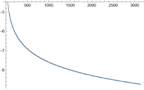
Figure 1. Plot of the imaginary part versus real part of the first 100 values $z$ with $\operatorname{Re}{z}>\pi$ for which $z^{2}$ is a resonance for $\alpha=0$ and $y_{3}=1$ in the Dirichlet half-space case.

4. Asymptotics of the Resonance Counting Function

In the present Section we study the asymptotic behaviour of the resonance counting function for the one center Laplacian in the half-space. Consider the set $\Sigma\Bigl{(}-\Delta_{\alpha,y}^{\textup{D}}\Bigr{)}$ of complex $z$ such that $z^{2}$ is an eigenvalue or a resonance of $-\Delta_{\alpha,y}^{\textup{D}}$. Let’s define

$$\mathcal{N}_{-\Delta_{\alpha,y}^{\textup{D}}}(R)=\#\Set{z\in\Sigma\Bigl{(}-\Delta_{\alpha,y}^{\textup{D}}\Bigr{)}}{\left\lvert z\right\rvert<R}$$

the counting function for the the elements of $\Sigma\Bigl{(}-\Delta_{\alpha,y}^{\textup{D}}\Bigr{)}$ counted with the appropriate multiplicity. We now prove that (see [27, 7] for an analogous result for $N$-point interactions in $\mathbb{R}^{n}$)

Proposition 4.1.

$\forall\alpha\in\mathbb{R}$ and $y\in\mathbb{R}^{3}_{+}$ it holds that

(4.1) $$\mathcal{N}_{-\Delta_{\alpha,y}^{\textup{D}}}(R)\sim 2\frac{y_{3}}{\pi}R\ \ \text{as}\ \ \ R\to\infty\ .$$

Remark 4.1.

We actually count solutions of $\Gamma_{\alpha,y}^{\textup{D}}(z)=0$. So the result is an consequence of well known properties of distribution of zeroes of exponential polynomials (see for example Section 2 in [27] and references therein), but here we give an independent direct proof.

Proof.

Let $z_{k}^{2}$ be the resonance of $-\Delta_{\alpha,y}^{\textup{D}}$ such that $\operatorname{Re}z_{k}:=a_{k}\in\Bigl{(}\frac{k\pi}{y_{3}},\frac{(2k+1)\pi}{2y_{3}}\Bigr{)}$ and $\{a_{k}\}_{k=1,2,\dots}$ the associated sequence. We start by proving that

(4.2) $$a_{k}\sim\frac{(2k+1/2)\pi}{2y_{3}}\ \ \ \ \text{as}\ \ \ k\to+\infty.$$

We observe that, even if it can occur that $a_{1}\in\Bigl{(}\frac{5\pi}{4y_{3}},\frac{3\pi}{2y_{3}}\Bigr{)}$, it still happens that, definitely in $k$, $a_{k}\in\Bigl{(}\frac{k\pi}{y_{3}},\frac{(2k+1/2)\pi}{2y_{3}}\Bigr{)}$. This is true because, recalling Eq. 3.8, we have that

$$g\biggl{(}\frac{(2k+1/2)\pi}{2y_{3}}\biggr{)}=\frac{1}{(2k+1/2)\pi}\quad\textup{and}\quad\lim_{a\to\frac{(2k+1/2)\pi}{2y_{3}}}h(a)=e^{-8\pi\alpha y_{3}}$$

and so there exists a $\overline{k}$, such that $\forall k\geq\overline{k}$, $g<h$ when both evaluated at the middle point of the $k$-th interval, which implies that the unique solution is in the first half of the interval.
Let $w$ be in $\Bigl{(}\frac{\overline{k}\pi}{y_{3}},\frac{(2\overline{k}+1/2)\pi}{2y_{3}}\Bigr{)}$ and $\{w_{l}\}_{l=0,1,\dots}=\Bigl{\{}w+\frac{2l\pi}{2y_{3}}\Bigr{\}}_{l=0,1,\dots}$. We have that

$$g(w_{l})=\frac{\sin{(2y_{3}w)}}{2y_{3}w+2l\pi}\quad\textup{and}\quad h(w_{l})=e^{-8\pi\alpha y_{3}-\frac{2y_{3}w+2l\pi}{\tan{(2y_{3}w)}}}.$$

Both sequences are vanishing, but $\{h(w_{l})\}$ faster than $\{g(w_{l})\}$, which implies that for sufficiently large $l$, $g(w_{l})>h(w_{l})$ and so the solution in the $(\overline{k}+l)$-th interval must be in $\Bigl{(}w_{l},\frac{(2(\overline{k}+l)+1/2)\pi}{2y_{3}}\Bigr{)}$. The arbitrarity of $w$ in $\Bigl{(}\frac{\overline{k}\pi}{y_{3}},\frac{(2\overline{k}+1/2)\pi}{2y_{3}}\Bigr{)}$ leads to Eq. 4.2.

So we have that $a_{k}=\frac{(2k+1/2)\pi}{2y_{3}}+o(1)$ for $k\to+\infty$. We use this property to estimate $\mathcal{N}_{-\Delta_{\alpha,y}^{\textup{D}}}(R)$ as $R\to+\infty$ excluding at most finitely many resonances. This is equivalent to find the highest $k$ for which

$$a_{k}^{2}+\frac{1}{4y_{3}^{2}}\ln^{2}{\Biggl{(}\frac{\sin{(2y_{3}a_{k})}}{2y_{3}a_{k}}\Biggr{)}}<R^{2}.$$

Substituting the asymptotic expression for $k\to+\infty$, we get

$$\biggl{(}2k+\frac{1}{2}\biggr{)}^{2}\pi^{2}+\ln^{2}{\Biggl{(}\biggl{(}2k+\frac{1}{2}\biggr{)}\pi\Biggr{)}}+o(1)<4y_{3}^{2}R^{2}.$$

If we set $s=\Bigl{(}2k+\frac{1}{2}\Bigr{)}\pi$, it becomes

$$s^{2}+\ln^{2}{(s)}+o(1)<4y_{3}^{2}R^{2}.$$

We are concerned about large value of $s$, so, since the left side happens to be increasing for $s$ sufficiently large, the largest $s$ satisfying the inequality will be the one satisfying

$$s^{2}+\ln^{2}{(s)}+o(1)=4y_{3}^{2}R^{2}.$$

We look for the asymptotic for $s$ solving the equation, when $R\to+\infty$. We write

(4.3) $$s=\sqrt{4y_{3}^{2}R^{2}-\ln^{2}{(s)}}+o(1).$$

We see that $s<2y_{3}R$ and $s=O(R)$. This implies that $\ln^{2}{(s)}=O\Bigl{(}\ln^{2}(R)\Bigr{)}$. Now we substitute this in Eq. 4.3, obtaining

$$s=2y_{3}R\sqrt{1+O\Biggl{(}\frac{\ln^{2}{(R)}}{R^{2}}}\Biggr{)}+o(1)=2y_{3}R+o(1).$$

And so for $k$ holds ($\lfloor\cdot\rfloor$ and $\{\cdot\}$ indicate respectively the integer part and the fractional part) $k=\Biggl{\lfloor}\frac{y_{3}}{\pi}R-\frac{1}{4}\Biggr{\rfloor}.$
But in this way we only counted the resonances with positive real part, so to count them all we just double the number:

(4.4) $$\mathcal{N}_{-\Delta_{\alpha,y}^{\textup{D}}}(R)\sim 2\Biggl{\lfloor}\frac{y_{3}}{\pi}R-\frac{1}{4}\Biggr{\rfloor}$$

giving finally equation (4.1) in the statement ∎

Remark 4.2.

From (4.1) or from (4.4) it follows

$$\begin{split}\lim_{R\to+\infty}\frac{\ln{\Bigl{(}\mathcal{N}_{-\Delta_{\alpha,y}^{\textup{D}}}(R)\Bigr{)}}}{\ln{R}}=1\end{split}$$

The analogous result proved in [15] for Schrödinger operators $-\Delta+V$ with bounded potentials with compact support in $\mathbb{R}^{n}$ gives

$$\lim_{R\to+\infty}\frac{\ln{\Bigl{(}\mathcal{N}_{-\Delta+V}(R)\Bigr{)}}}{\ln{R}}=n$$

showing a dependence on the dimension different from the one obtained here. This different behavior was already noticed in [27] for finitely many point interactions in $\mathbb{R}^{3}$, and compared with the analogous behavior on quantum graphs. See also the earlier work [36]. The reason of this anomalous behavior is not immediately interpretable, in view of the known fact that point interactions are singular limit of standard Schrödinger operators with rescaled smooth potentials (see for example [2]).

Remark 4.3.

The same result holds also for $\mathcal{N}_{-\Delta_{\alpha,y}^{\textup{N}}}(R)$. The proof for the Neumann case follows closely the one given above and it will be omitted.

5. Resonance Expansion for the Wave and Schrödinger Equation with Point Interaction

In the present Section, we prove the resonance expansion for the solution of the wave equation and for the propagator of the Schrödinger equation on the half-space in the presence of a point interaction.
As regards the wave equation, a similar analysis in the presence of a smooth $L_{\textup{comp}}^{\infty}(\mathbb{R}^{n})$ potential on the whole space is given in [21] (pages 39-45 and 110-111). We recall that $L^{\infty}_{\textup{comp}}(\mathbb{R}^{n})$ is the space of measurable, essentially bounded functions with compact support. In the following Theorem we will treat the abstract wave equation with generator given by a point interaction in $\mathbb{R}^{3}_{+}$ and initial data in $L^{2}_{\textup{comp}}(\mathbb{R}^{3}_{+})$ and $H^{1}_{\textup{comp}}(\mathbb{R}^{3}_{+})$, the space of square integrable function in $\mathbb{R}^{3}_{+}$ with compact support and the corresponding Sobolev space of order one. The restriction to data with compact support is needed, as in the standard case, to tame the exponentially diverging behavior of resonance at spatial infinity.

Theorem 5.1.

Let $\alpha\in\mathbb{R}$, $y=(y_{1},y_{2},y_{3})\in\mathbb{R}_{+}^{3}$ and suppose $w(t)$ is the solution of

(5.1) $$\begin{cases}\biggl{(}\frac{\partial^{2}}{\partial t^{2}}-\Delta_{\alpha,y}^{\textup{D}}\biggr{)}w(t)=0\\ w(0)=w_{0}\in H_{\textup{comp}}^{1}(\mathbb{R}_{+}^{3})\\ \frac{\partial w}{\partial t}(0)=w_{1}\in L_{\textup{comp}}^{2}(\mathbb{R}_{+}^{3})\end{cases}.$$

Let $\Set{z_{j}^{2}}$ and $\lambda$ be respectively the set of resonances and the possible eigenvalue of $\Delta_{\alpha,y}^{\textup{D}}$, and $R(z):=\Bigl{(}-\Delta_{\alpha,y}^{\textup{D}}-z^{2}\Bigr{)}^{-1}$ Then, for any $A>0$,

• if $\alpha\neq-\frac{1}{8\pi y_{3}}$

  $$w(t)=\sum_{\set{\operatorname{Im}{z_{j}}>-A}}e^{-iz_{j}t}f_{j}+\quad E_{A}(t),$$

  where the sum is finite and

  (5.2) $$f_{j}=-\operatorname{Res}_{z=z_{j}}{\biggl{(}iR(z)w_{1}+zR(z)w_{0}\biggr{)}};$$

• if $\alpha=-\frac{1}{8\pi y_{3}}$

  $$w(t)=\sum_{\set{\operatorname{Im}{z_{j}}>-A}}e^{-iz_{j}t}f_{j}+f_{0,0}+tf_{0,1}+\quad E_{A}(t),$$

  where the sum is finite, $f_{j}$ are still defined as in Eq. 5.2 and

  $$f_{0,0}+tf_{0,1}=-\operatorname{Res}_{z=0}{\biggl{(}iR(z)w_{1}+zR(z)w_{0}\biggr{)}}.$$

Moreover, for any compact, connected set $K$ such that $\operatorname{supp}{(w_{j})}\subset K$, $j=0,1$, there exist constants $C_{K,A}$ and $T_{K,A}$ such that

$$\left\lVert E_{A}(t)\right\rVert_{H^{2}(K)}\leq C_{K,A}e^{-tA}(\left\lVert w_{0}\right\rVert_{H^{1}(K)}+\left\lVert w_{1}\right\rVert_{L^{2}(K)}),\quad t\geq T_{K,A}.$$

The following technical lemma allows to bound on the meromorphically continued resolvent on $\mathbb{C}_{-}$ when smoothly truncated by means of a cutoff function $\rho$.

Lemma 5.1.

Let $\alpha\in\mathbb{R}$ and $y=(y_{1},y_{2},y_{3})\in\mathbb{R}_{+}^{3}$ and $K\subset\mathbb{R}_{+}^{3}$ compact. For any $\rho\in C_{0}^{\infty}(\mathbb{R}_{+}^{3})$ there exist constants $A,C$ and $T$ depending on $\rho$ such that

(5.3) $$\left\lVert\rho(-\Delta_{\alpha,y}^{\textup{D}}-z^{2})^{-1}\rho\right\rVert_{L^{2}(K)\to H^{j}(K)}\leq C(1+\left\lvert z\right\rvert)^{j-1}e^{T(\operatorname{Im}{z})_{-}},\ \ \ j=0,1,2$$

for

$$\operatorname{Im}{z}\geq-A-\delta\ln{(1+\left\lvert z\right\rvert)},\quad\left\lvert z\right\rvert>C_{0},\quad\delta<\frac{1}{2y_{3}}$$

where $z^{2}$ is not a resonance and it is denoted $(x)_{-}=\max\Set{-x,0}$.

Proof.

We start by proving that for any $A>0$ there are only finitely many resonances in the region

(5.4) $$\Set{z\in\mathbb{C}}{\operatorname{Im}{z}\geq-A-\delta\ln{(1+\left\lvert z\right\rvert)}}\ .$$

As shown previously, all resonances are on the curve Eq. 3.1. This means that the curve

(5.5) $$\operatorname{Im}{z}=\frac{1}{2y_{3}}\ln{\Biggl{(}\frac{1}{2y_{3}\left\lvert\operatorname{Re}{z}\right\rvert}\Biggr{)}}\ \ \ \ \ \text{equivalent to}\ \ \ \ \left\lvert\operatorname{Re}{z}\right\rvert=\frac{1}{2y_{3}}e^{-2y_{3}\operatorname{Im}{z}}$$

is above all resonances. The equation of the curve which delimits the region Eq. 5.4 can be written in explicit form as follows

(5.6) $$\left\lvert\operatorname{Re}{z}\right\rvert=\sqrt{\biggl{(}e^{-\frac{\operatorname{Im}{z}+A}{\delta}}-1\biggr{)}^{2}-\Bigl{(}\operatorname{Im}{z}\Bigr{)}^{2}}.$$

Both curves are symmetric with respect to the imaginary axis, so we limit ourself to $\operatorname{Re}{z}>0$. If it happens that for $\operatorname{Im}{z}$ large enough, curve Eq. 5.6 is above curve Eq. 5.5, then for $\operatorname{Im}{z}$ large enough all $z$ which generate a resonance and obey this constraint are below Eq. 5.6 and hence only a finite quantity of them is in the region described by Eq. 5.4. This scenario happens for $\frac{1}{\delta}>2y_{3}$ regardless of the value of $A$.

In order to prove Eq. 5.3 we use Eq. 2.9 and write

(5.7) $$\left\lVert\rho(-\Delta_{\alpha,y}^{\textup{D}}-z^{2})^{-1}\rho\right\rVert_{L^{2}(K)\to H^{j}(K)}\leq\left\lVert\rho(-\Delta^{\textup{D}}-z^{2})^{-1}\rho\right\rVert_{L^{2}(K)\to H^{j}(K)}\\ +\left\lvert\Gamma_{\alpha,y}^{\mathbb{R}_{+}^{3},\textup{D}}(z)\right\rvert^{-1}\left\lVert\rho G_{z,y}^{\textup{D}}(-\Delta^{\textup{D}}-z^{2})^{-1}\rho\right\rVert_{L^{2}(K)\to H^{j}(K)}.$$

We recall the following bound for the free truncated resolvent ([21] Theorem 3.1)

$$\left\lVert\rho(-\Delta-z^{2})^{-1}\rho\right\rVert_{L^{2}(K)\to H^{j}(K)}\leq C(1+\left\lvert z\right\rvert)^{j-1}e^{T(\operatorname{Im}{z})_{-}},\quad j=0,1,2,$$

where $L>\operatorname{diam}{(\operatorname{supp}{(\rho)})}$ and that is also valid if we replace $-\Delta$ with $-\Delta^{\textup{D}}$. This directly bounds the first term in Eq. 5.7. It does the same for the second one if we observe that $G_{z,y}^{\textup{D}}$ is in $L_{\textup{loc}}^{2}(\mathbb{R}_{+}^{3})$ and that outside of resonances $\left\lvert\Gamma_{\alpha,y}^{\mathbb{R}_{+}^{3},\textup{D}}(z)\right\rvert^{-1}$ is bounded. Hence Eq. 5.3 follows. ∎

Proof of Theorem 5.1.

We start by considering the case $w_{0}=0$ and $\operatorname{supp}{(w_{1})}\subset K$.

By the functional calculus, the propagator of Eq. 5.1 can be written as

(5.8) $$U(t)=\int_{0}^{+\infty}\frac{\sin{tz}}{z}\mathop{}\!\mathrm{d}E_{z}+\frac{\sin{t\lambda}}{\lambda}\biggl{(}\cdot,G_{\sqrt{\lambda},y}^{\textup{D}}\biggr{)}G_{\sqrt{\lambda},y}^{\textup{D}}.$$

If $\lambda=0$ is an eigenvalue (case $ii)$ in the statement), the last term is replaced by

$$t\,\biggl{(}\cdot,G_{0,y}^{\textup{D}}\biggr{)}G_{0,y}^{\textup{D}}.$$

Since for $z$ near $\lambda\neq 0$, $R(z)=(\lambda^{2}-z^{2})^{-1}\biggl{(}\cdot,G_{\sqrt{\lambda},y}^{\textup{D}}\biggr{)}G_{\sqrt{\lambda},y}^{\textup{D}}+Q(z)$, where $Q(z)$ is holomorphic near $\lambda$ and $\operatorname{Res}_{z=\lambda}{(\lambda^{2}-z^{2})}=-(2\lambda)^{-1}$, we have

(5.9) $$\frac{\sin{t\lambda}}{\lambda}\biggl{(}\cdot,G_{\sqrt{\lambda},y}^{\textup{D}}\biggr{)}G_{\sqrt{\lambda},y}^{\textup{D}}=-\operatorname{Res}_{z=\lambda}{(iR(z)e^{-izt})}-\operatorname{Res}_{z=-\lambda}{(iR(-z)e^{-izt})}=\Pi_{\lambda}+\Pi_{-\lambda}.$$

If $\lambda=0$, instead

(5.10) $$t\,\biggl{(}\cdot,G_{0,y}^{\textup{D}}\biggr{)}G_{0,y}^{\textup{D}}=-t\operatorname{Res}_{z=0}{(iR(z))}.$$

In the following, the term for $\lambda=0$ will not be reported whenever it is not needed to distinguish the two cases.

By Stone’s formula for the spectral measure $\mathop{}\!\mathrm{d}E_{z}$ in terms of $R(z)$, we have

$$\mathop{}\!\mathrm{d}E_{z}=\frac{1}{\pi i}(R(z)-R(-z))z\mathop{}\!\mathrm{d}z.$$

Hence

$$\begin{split}w(t,x)-\frac{\sin{t\lambda}}{\lambda}\biggl{(}\cdot,G_{\sqrt{\lambda},y}^{\textup{D}}\biggr{)}G_{\sqrt{\lambda},y}^{\textup{D}}&=\frac{1}{\pi i}\int_{0}^{+\infty}\sin{tz}(R(z)-R(-z))w_{1}(x)\mathop{}\!\mathrm{d}z\\ &=\frac{1}{2\pi}\lim_{\varepsilon\to 0^{+}}\int_{\mathbb{R}\setminus(-\varepsilon,\varepsilon)}e^{-itz}(R(z)-R(-z))w_{1}(x)\mathop{}\!\mathrm{d}z\\ &\begin{multlined}=\frac{1}{2\pi}\int_{\Sigma_{\varepsilon_{0}}}e^{-itz}(R(z)-R(-z))w_{1}(x)\mathop{}\!\mathrm{d}z\\ +\frac{1}{2\pi}\lim_{\varepsilon\to 0^{+}}\int_{\sigma_{\varepsilon}}e^{-itz}(R(z)-R(-z))w_{1}(x)\mathop{}\!\mathrm{d}z,\end{multlined}=\frac{1}{2\pi}\int_{\Sigma_{\varepsilon_{0}}}e^{-itz}(R(z)-R(-z))w_{1}(x)\mathop{}\!\mathrm{d}z\\ +\frac{1}{2\pi}\lim_{\varepsilon\to 0^{+}}\int_{\sigma_{\varepsilon}}e^{-itz}(R(z)-R(-z))w_{1}(x)\mathop{}\!\mathrm{d}z,\end{split}$$

where $\varepsilon_{0}$ is such that there are no non-zero poles of $R(z)$ in $D(0,\varepsilon_{0})$, $\Sigma_{\varepsilon_{0}}$ is the union of $\mathbb{R}\setminus(-\varepsilon_{0},\varepsilon_{0})$ with the semicircle in the upper complex half-plane of radius $\varepsilon_{0}$ and centered at zero oriented counterclockwise. $\sigma_{\varepsilon}$ instead is the semicircle in the upper complex half-plane of radius $\varepsilon$, centered at zero and oriented clockwise.

To prove that the integrand decays fast enough for the integral on $\Sigma_{\varepsilon_{0}}$ to be convergent we observe that, by the definition of $R(z)$, it follows that

$$\Bigl{(}R(z)-R(-z)\Bigr{)}\biggl{(}-\Delta_{\alpha,y}^{\textup{D}}\biggr{)}=(R(z)-R(-z))\biggl{(}-\Delta_{\alpha,y}^{\textup{D}}-z^{2}+z^{2}\biggr{)}=z^{2}\Bigl{(}R(z)-R(-z)\Bigr{)}.$$

From this we can conclude that for $\rho\in C_{0}^{\infty}(\mathbb{R}_{+}^{3})$ equal to one on $\operatorname{supp}{(w_{1})}$,

$$\begin{split}\rho\Bigl{(}R(z)-R(-z)\Bigr{)}\biggl{(}1-\Delta_{\alpha,y}^{\textup{D}}\biggr{)}\rho w_{1}&=\rho\Bigl{(}R(z)-R(-z)\Bigr{)}w_{1}+\rho\Bigl{(}R(z)-R(-z)\Bigr{)}\biggl{(}-\Delta_{\alpha,y}^{\textup{D}}\biggr{)}w_{1}\\ &=(1+z^{2})\rho\Bigl{(}R(z)-R(-z)\Bigr{)}w_{1}\end{split}$$

and so

(5.11) $$\rho\Bigl{(}R(z)-R(-z)\Bigr{)}\rho w_{1}=\rho\Bigl{(}R(z)-R(-z)\Bigr{)}(1+z^{2})^{-1}\biggl{(}1-\Delta_{\alpha,y}^{\textup{D}}\biggr{)}\rho w_{1}.$$

Since $\rho\Bigl{(}R(z)-R(-z)\Bigr{)}\rho=O(|z|^{-2})$ as $|z|\to\infty$ as an operator $L^{2}(\mathbb{R}_{+}^{3})\to L^{2}(\mathbb{R}_{+}^{3})$, this shows that the integral converges in $L_{\textup{loc}}^{2}(\mathbb{R}_{+}^{3})$.

The resolvent is holomorphic in a neighborhhod of the origin and hence the integral over $\sigma_{\varepsilon}$ converges to $0$ as $\varepsilon\to 0^{+}$, unless zero is an eigenvalue for $-\Delta_{\alpha,y}^{\textup{D}}$. In that case, we study the expression $R(z)-R(-z)$ near zero. We recall that $0$ is an eigenvalue if and only if $\alpha=-\frac{1}{8\pi y_{3}}$. In this case

$$R(z)-R(-z)=\frac{e^{iz\left\lvert x-y\right\rvert}}{4\pi\left\lvert x-y\right\rvert}\frac{e^{iz\left\lvert x^{\prime}-y\right\rvert}}{4\pi\left\lvert x^{\prime}-y\right\rvert}\Bigl{(}\Gamma_{\alpha,y}^{\textup{D}}(z)\Bigr{)}^{-1}-\frac{e^{-iz\left\lvert x-y\right\rvert}}{4\pi\left\lvert x-y\right\rvert}\frac{e^{-iz\left\lvert x^{\prime}-y\right\rvert}}{4\pi\left\lvert x^{\prime}-y\right\rvert}\Bigl{(}\Gamma_{\alpha,y}^{\textup{D}}(-z)\Bigr{)}^{-1}.$$

Some computations show that

$$\operatorname{Res}_{z=0}{\Bigl{(}R(z)-R(-z)\Bigr{)}}=\frac{i}{\pi y_{3}\left\lvert x-y\right\rvert\left\lvert x^{\prime}-y\right\rvert}\Biggl{(}\frac{y_{3}}{3}-\frac{\left\lvert x-y\right\rvert+\left\lvert x^{\prime}-y\right\rvert}{2}\Biggr{)},$$

which means that

$$\begin{split}\frac{1}{2\pi}\lim_{\varepsilon\to 0^{+}}\int_{\sigma_{\varepsilon}}e^{-itz}(R(z)-R(-z))w_{1}(x)\mathop{}\!\mathrm{d}z&=\frac{w_{1}(x)}{2\pi y_{3}\left\lvert x-y\right\rvert\left\lvert x^{\prime}-y\right\rvert}\Biggl{(}\frac{y_{3}}{3}-\frac{\left\lvert x-y\right\rvert+\left\lvert x^{\prime}-y\right\rvert}{2}\Biggr{)}\\ &=\Pi_{0}w_{1}(x).\end{split}$$

Let $\rho\in C_{0}^{\infty}(\mathbb{R}_{+}^{3})$ satisfy $\rho=1$ on $K$. We choose $r$ large enough so that all the resonances $z^{2}$ with $\operatorname{Im}{z}>-A-\delta\ln{(1+\left\lvert\operatorname{Re}{z}\right\rvert)}$ are contained in the ball $\left\lvert z\right\rvert\leq r$. We deform the contour of integration in the integral over $\Sigma_{\varepsilon_{0}}$ using the following contours:

(5.12) $$\omega_{r}=\Set{s-i\,\Bigl{(}A+\varepsilon+\delta\ln{(1+\left\lvert s\right\rvert)}\Bigr{)}}{s\in[-r,r]}$$

(5.13) $$\gamma_{r}^{\pm}=\Set{\pm r-is}{0\leq s\leq A+\varepsilon+\delta\ln{(1+r)}},\quad\gamma_{r}=\gamma_{r}^{+}\cup\gamma_{r}^{-}$$

(5.14) $$\gamma_{r}^{\infty}=(-\infty,r)\cup(r,+\infty).$$

$\varepsilon$ is chosen in such a way that $\omega_{r}$ does not cross resonances. We also define

$$\Omega_{A}=\Set{z}{\operatorname{Im}{z}\geq-A-\varepsilon-\delta\ln{(1+\left\lvert\operatorname{Re}{z}\right\rvert)}}\setminus\Set{0}$$

and define

$$\Pi^{\prime}_{A}(t)=\sum_{\Set{z_{j}\in\Omega_{A}}\cup\Set{z_{j}=\pm\lambda}}\operatorname{Res}_{z=z_{j}}{\Bigl{(}\rho R(z)\rho e^{-izt}\Bigr{)}}.$$

By combining Eq. 5.8, Eq. 5.9 (or Eq. 5.10 when zero is an eigenvalue) and the residue theorem, we can write that

(5.15) $$\rho U(t)\rho=\Pi^{\prime}_{A}(t)+E_{\omega_{r}}(t)+E_{\gamma_{r}}(t)+E_{\gamma_{r}^{\infty}}(t)+\Pi_{\lambda}+\Pi_{-\lambda},$$

where

$$E_{\gamma}(t)=\frac{1}{2\pi}\int_{\gamma}e^{-itz}\rho\Bigl{(}R(z)-R(-z)\Bigr{)}\rho w_{1}\mathop{}\!\mathrm{d}z.$$

We note that $\Pi_{\lambda}+\Pi_{-\lambda}$ cancels out with the term in $\Pi^{\prime}_{A}$ containing the residue at $z=\pm\lambda$. So, by putting together this cancellations in the new term, $\Pi_{A}$, Eq. 5.15 becomes

(5.16) $$\rho U(t)\rho=\Pi_{A}(t)+E_{\omega_{r}}(t)+E_{\gamma_{r}}(t)+E_{\gamma_{r}^{\infty}}(t).$$

Now we prove that the the last two terms in Eq. 5.15 are negligible in the limit $r\to+\infty$. To do so, we consider $w_{1}\in H^{2}(K)$. This allows us to use Eq. 5.11 to Eq. 5.3 with $j=1$ and obtain the following bound

(5.17) $$\begin{split}\left\lVert E_{\gamma_{r}^{\infty}}(t)w_{1}\right\rVert_{H^{1}(K)}&\leq C\left\lVert\int_{r}^{+\infty}e^{-itz}\rho\Bigl{(}R(z)-R(-z)\Bigr{)}\rho w_{1}\mathop{}\!\mathrm{d}z\right\rVert_{H^{1}(K)}\\ &\leq C\left\lVert\int_{r}^{+\infty}\rho\Bigl{(}R(z)-R(-z)\Bigr{)}(1+z^{2})^{-1}\Bigl{(}1-\Delta_{\alpha,y}^{\textup{D}}\Bigr{)}\rho w_{1}\mathop{}\!\mathrm{d}z\right\rVert_{H^{1}(K)}\\ &\leq C\int_{r}^{+\infty}(1+z^{2})^{-1}\left\lVert w_{1}\right\rVert_{H^{2}(K)}\mathop{}\!\mathrm{d}z=C\biggl{(}\frac{\pi}{2}-\arctan{r}\biggr{)}\left\lVert w_{1}\right\rVert_{H^{2}(K)}\xrightarrow[r\to+\infty]{}0.\end{split}$$

Instead, for the other term and for $t>T$ one has

$$\begin{split}\left\lVert E_{\gamma_{r}}(t)w_{1}\right\rVert_{H^{1}(K)}&=C\left\lVert-i\int_{0}^{A+\varepsilon+\delta\ln{(1+r)}}e^{-it(r-is)}\rho\Bigl{(}R(r-is)-R(-r+is)\Bigr{)}\rho w_{1}\mathop{}\!\mathrm{d}s\right\rVert_{H^{1}(K)}\\ &\textup{\footnotesize$\leq C\left\lVert\int_{0}^{A+\varepsilon+\delta\ln{(1+r)}}e^{-it(r-is)}\rho\Bigl{(}R(r-is)-R(r+is)\Bigr{)}(1+(r-is)^{2})^{-1}\Bigl{(}1-\Delta_{\alpha,y}^{\textup{D}}\Bigr{)}\rho w_{1}\mathop{}\!\mathrm{d}s\right\rVert_{H^{1}(K)}$}\\ &\leq C\int_{0}^{A+\varepsilon+\delta\ln{(1+r)}}(1+(r-is)^{2})^{-1}e^{-(t-T)s}\left\lVert w_{1}\right\rVert_{H^{2}(K)}\mathop{}\!\mathrm{d}s\\ &\leq C\int_{0}^{A+\varepsilon+\delta\ln{(1+r)}}(1+(r-is)^{2})^{-1}\left\lVert w_{1}\right\rVert_{H^{2}(K)}\mathop{}\!\mathrm{d}s\\ &=C\Biggl{(}\arctan{\biggl{(}r-i\Bigl{(}A+\varepsilon+\delta\ln{(1+r)}\Bigr{)}\biggr{)}}-\arctan{r}\Biggr{)}\left\lVert w_{1}\right\rVert_{H^{2}(K)}\xrightarrow[r\to+\infty]{}0.\end{split}$$

We have now proved that

$$\rho U(t)\rho=\Pi_{A}(t)+E_{\omega}(t),\quad\textup{for}\quad w_{1}\in H^{2}(K)$$

($\omega$ is the curve $\omega=\Set{s-i\,\Bigl{(}A+\varepsilon+\delta\ln{(1+\left\lvert s\right\rvert)}\Bigr{)}}{s\in\mathbb{R}}$).

We now show that for $t\gg 1$ and $w_{1}\in H^{2}(K)$ holds that

(5.18) $$\left\lVert E_{\omega}(t)w_{1}\right\rVert_{H^{2}(K)}\leq Ce^{-tA}\left\lVert w_{1}\right\rVert_{L^{2}(K)}.$$

In order to do so, we use Eq. 5.3 with $j=2$ and the assumption that there exist a compact set containing $\omega$ in which there are no poles of $R(z)$. We obtain

$$\begin{split}\left\lVert E_{\omega}(t)w_{1}\right\rVert_{H^{2}(K)}&\leq Ce^{-tA}\int_{-\infty}^{+\infty}e^{-t\delta\ln{(1+\left\lvert s\right\rvert)}}(1+\left\lvert s\right\rvert)e^{T\delta\ln{(1+\left\lvert s\right\rvert)}}\left\lVert w_{1}\right\rVert_{L^{2}(K)}\mathop{}\!\mathrm{d}s\\ &=Ce^{-tA}\int_{-\infty}^{+\infty}(1+\left\lvert s\right\rvert)^{-(t-T)\delta+1}\left\lVert w_{1}\right\rVert_{L^{2}(K)}\mathop{}\!\mathrm{d}s.\end{split}$$

This last integral is finite if $-(t-T)\delta+1<-1$, which is equivalent to $t>T+\frac{2}{\delta}$.

In Eq. 5.18 the above bound is in terms of the $L^{2}(K)$ norm of $w_{1}$ for $w_{1}\in H^{2}(K)$. Since, $H^{2}(K)$ is dense in $L^{2}(K)$, then the same bound holds for any $w_{1}\in L^{2}(K)$ and the theorem holds for any $w_{1}\in L^{2}(K)$.

The proof for arbitrary $w_{0}\in H_{\textup{comp}}^{1}(\mathbb{R}_{+}^{3})$ and $w_{1}=0$ follows the same steps, with the replacement $\sin{tz}/z\longrightarrow\cos{tz}$ in the formula for $w(t,x)$. ∎

Now we turn to the Schrödinger equation. In this case, instead of giving the resonance expansion of the solution, we give the expansion of the kernel of the propagator, equivalent from the mathematical point of view and typically more useful in many applications in Quantum Mechanics. Previous early analysis of this kind has been given in [1], where the case of $\mathbb{R}^{3}$ with several point interactions or infinitely many point interactions periodically placed is treated. In the following theorem we consider the resonance expansion for the propagator of the absolutely continuous part of the Hamiltonian of a point interaction on the half-space. For the sake of simplicity in the exposition we exclude in the statement and proof the case where a zero energy eigenvalue is present. This, however, can be treated straightforwardly as already done for the wave equation.
The next Theorem treats the Dirichlet case, completely analogous result and proof hold true for Neumann boundary conditions.

Proposition 5.1.

Let $H=-\Delta_{\alpha,y}^{\textup{D}}$ with $\alpha\neq-\frac{1}{8\pi y_{3}}$ and $H^{+}$ its projection on the absolutely continuous spectrum. Then there exists some $t_{0}(x,x^{\prime},\alpha,y)$ such that for $t>t_{0}$ the following expansion holds

(5.19) $$\begin{split}e^{-itH_{+}}(x,x^{\prime})&=(2\pi it)^{-\frac{3}{2}}e^{\frac{i}{2t}\left\lvert x-x^{\prime}\right\rvert^{2}}+\sum_{n}2z_{n}e^{-itz_{n}^{2}}\operatorname{Res}_{z=z_{n}}{\biggl{(}\Bigl{(}\Gamma^{\textup{D}}_{\alpha,y}(z)\Bigr{)}^{-1}\biggr{)}}G^{\textup{D}}_{z_{n},y}(x)G^{\textup{D}}_{z_{n},y}(x^{\prime})\\ &-\frac{1}{2\pi}\int_{0}^{+\infty}\biggl{(}\hat{R}\Bigl{(}e^{-i\frac{\pi}{4}}s\Bigr{)}-\hat{R}\Bigl{(}-e^{-i\frac{\pi}{4}}s\Bigr{)}\biggr{)}e^{-ts}\mathop{}\!\mathrm{d}s,\end{split}$$

with $\hat{R}(z)=(H-z^{2})^{-1}-(-\Delta^{D}-z^{2})^{-1}$. The sum in Eq. 5.19 is taken over all $z_{n}$ lying in the region $-\frac{\pi}{4}<\operatorname{Arg}{k}<0$ such that $z_{n}^{2}$ is a resonance.

Proof.

By the definition of $\hat{R}$ and functional calculus it holds

$$e^{-itH_{+}}(x,x^{\prime})=-\frac{1}{2\pi i}\int_{0}^{+\infty}e^{-itz^{2}}\hat{R}(z)(x,x^{\prime})2z\mathop{}\!\mathrm{d}z-\frac{1}{2\pi i}\int_{0}^{+\infty}e^{-itz^{2}}G_{z,y}^{\textup{D}}(x,x^{\prime})2z\mathop{}\!\mathrm{d}z.$$

It holds that

$$\frac{1}{2\pi i}\int_{0}^{+\infty}e^{-itz^{2}}G_{z,y}^{\textup{D}}(x,x^{\prime})2z\mathop{}\!\mathrm{d}z=(2\pi it)^{-\frac{3}{2}}e^{i\left\lvert x-x^{\prime}\right\rvert^{2}{2t}}.$$

Instead, because of the parity of $\hat{R}(z)$, we can rewrite the other integral as

$$-\frac{1}{2\pi i}\int_{0}^{+\infty}e^{-itz^{2}}\Bigl{(}\hat{R}(z)-\hat{R}(-z)\Bigr{)}(x,x^{\prime})2z\mathop{}\!\mathrm{d}z.$$

Using the residue theorem, this integral can be decomposed as

(5.20) $$\begin{split}\frac{1}{2\pi i}\int_{C_{R}}e^{-itz^{2}}\Bigl{(}\hat{R}(z)-\hat{R}(-z)\Bigr{)}(x,x^{\prime})2z\mathop{}\!\mathrm{d}z\ +\ &\frac{1}{2\pi i}\int_{\gamma_{R}}e^{-itz^{2}}\Bigl{(}\hat{R}(z)-\hat{R}(-z)\Bigr{)}(x,x^{\prime})2z\mathop{}\!\mathrm{d}z\\ +\ &\sum_{n}2z_{n}e^{-itz_{n}^{2}}\operatorname{Res}_{z=z_{n}}{\Bigl{(}\hat{R}(z)-\hat{R}(-z)\Bigr{)}}(x,x^{\prime}),\end{split}$$

where $C_{R}$ is the arc of circumference of radius $R$ going clockwise from $z=R$ to $z=Re^{-i\pi/4}$, $\gamma_{R}$ is the segment going from $z=Re^{-i\pi/4}$ towards the origin and the sum is over the $z_{n}$ in the region delimited by $C_{R}$, $\gamma_{R}$ and the real positive semiaxis.

We prove that the integral over $C_{R}$ vanishes for $R\to+\infty$. We prove this just for the term with $\hat{R}(z)$. Analogous observations prove the same for $\hat{R}(-z)$. By Proposition 3.1, there are infinite resonances $z_{n}$ and $\left\lvert z_{n}\right\rvert\to+\infty$ for $n\to+\infty$. This means that, in order to study the limit $R\to+\infty$, we have to distinguish the cases

• $R\neq\left\lvert z_{n}\right\rvert$, $\forall n\in\mathbb{N}$;

• $R=\left\lvert z_{n}\right\rvert$, for some $n\in\mathbb{N}$.

In the former case, the integral is given by

(5.21) $$\int_{C_{R}}e^{-itz^{2}}\biggl{(}\alpha-\frac{iz}{4\pi}+\frac{e^{2izy_{3}}}{8\pi y_{3}}\biggr{)}^{-1}\frac{e^{iz\left\lvert x-y\right\rvert}}{4\pi\left\lvert x-y\right\rvert}\frac{e^{iz\left\lvert x^{\prime}-y\right\rvert}}{4\pi\left\lvert x^{\prime}-y\right\rvert}2z\mathop{}\!\mathrm{d}z.$$

We substitute $z=Re^{i\theta}$ and estimate the absolute value of the integrand

$$\left\lvert e^{-itR^{2}e^{2i\theta}}\biggl{(}\alpha-\frac{iRe^{i\theta}}{4\pi}+\frac{e^{2iRe^{i\theta}y_{3}}}{8\pi y_{3}}\biggr{)}^{-1}\frac{e^{iRe^{i\theta}\left\lvert x-y\right\rvert}}{4\pi\left\lvert x-y\right\rvert}\frac{e^{iRe^{i\theta}\left\lvert x^{\prime}-y\right\rvert}}{4\pi\left\lvert x^{\prime}-y\right\rvert}2ie^{i\theta}R^{2}\right\rvert=\left\lvert I\right\rvert.$$

The second factor is bounded, because the path does not cross any resonance, hence it holds that

$$\left\lvert I\right\rvert\leq C(x,x^{\prime},y)R^{2}e^{R\sin{\theta}(2tR\cos{\theta}-\left\lvert x-y\right\rvert-\left\lvert x^{\prime}-y\right\rvert)}.$$

Since we are in the complex lower half-plane, $\sin{\theta}<0$. So if the other factor in the exponent is positive, then in the limit the integral vanishes. By recalling that $-\frac{\pi}{4}<\theta<0$, we have that

$$2tR\cos{\theta}-\left\lvert x-y\right\rvert-\left\lvert x^{\prime}-y\right\rvert>\sqrt{2}Rt-\left\lvert x-y\right\rvert-\left\lvert x^{\prime}-y\right\rvert,$$

which is positive for $t>\frac{\sqrt{2}}{2R}\Bigl{(}\left\lvert x-y\right\rvert+\left\lvert x^{\prime}-y\right\rvert\Bigr{)}$ and hence the integral vanishes in the limit.

In the other case, the path of integration has to be modified because the previous path would pass across the pole $z_{n}$. So, the integral Eq. 5.21 has to be replaced by the following sum of integrals of the same function

$$-\frac{1}{2\pi i}\int_{C_{R}^{1}}\dots\mathop{}\!\mathrm{d}z-\frac{1}{2\pi i}\int_{C_{\varepsilon}}\dots\mathop{}\!\mathrm{d}z-\frac{1}{2\pi i}\int_{C_{R}^{2}}\dots\mathop{}\!\mathrm{d}z,$$

where $C_{\varepsilon}$ is the semicircle of radius $\varepsilon$ centered at $z_{n}$, $C_{R}^{1}$ is the arc of circle of radius $R$ centered at the origin starting at $Re^{-i\frac{\pi}{4}}$ and ending when intersecting $C_{\varepsilon}$, and $C_{R}^{2}$ is the arc of circle of radius $R$ centered at the origin between the point $R$ and the intersection with $C_{\varepsilon}$. The path is run clockwise. The integrals on $C_{R}^{1}$ and $C_{R}^{2}$ are proven to vanish in the limit $n\to+\infty$ for $t$ large enough in the same way as in the first case. We consider the remaining integral, it holds that

$$-\frac{1}{2\pi i}\int_{C_{\varepsilon}}\dots\mathop{}\!\mathrm{d}z=-\frac{1}{2}\operatorname{Res}_{z=z_{n}}{\Biggl{(}e^{-itz^{2}}\biggl{(}\alpha-\frac{iz}{4\pi}+\frac{e^{2izy_{3}}}{8\pi y_{3}}\biggr{)}^{-1}\frac{e^{iz\left\lvert x-y\right\rvert}}{4\pi\left\lvert x-y\right\rvert}\frac{e^{iz\left\lvert x^{\prime}-y\right\rvert}}{4\pi\left\lvert x^{\prime}-y\right\rvert}2z\Biggr{)}}.$$

In order to find the residue, we study the divergent term

$$\Bigl{(}\Gamma_{\alpha,y}^{\textup{D}}(z)\Bigr{)}^{-1}=\biggl{(}\alpha-\frac{iz}{4\pi}+\frac{e^{2izy_{3}}}{8\pi y_{3}}\biggr{)}^{-1}.$$

Using the definition of $z_{n}$ we have that

$$\begin{split}\Bigl{(}\Gamma_{\alpha,y}^{\textup{D}}(z)\Bigr{)}&=\alpha-\frac{i}{4\pi}(z-z_{n})-\frac{iz_{n}}{4\pi}+\frac{e^{2iy_{3}(z-z_{n})}}{8\pi y_{3}}e^{2iy_{3}z_{n}}\\ &=\frac{e^{2iy_{3}z_{n}}}{8\pi y_{3}}\biggl{(}e^{2iy_{3}(z-z_{n})}-1\biggr{)}-\frac{i}{4\pi}(z-z_{n})\\ &=\frac{e^{2iy_{3}z_{n}}}{8\pi y_{3}}\sum_{k=1}^{+\infty}\frac{2^{k}i^{k}y_{3}^{k}}{k!}(z-z_{n})^{k}-\frac{i}{4\pi}(z-z_{n})\\ &=\frac{i}{4\pi}\biggl{(}e^{2iy_{3}z_{n}}-1\biggr{)}(z-z_{n})+O((z-z_{n})^{2}).\end{split}$$

This means that

$$\operatorname{Res}_{z=z_{n}}{\biggl{(}\Bigl{(}\Gamma_{\alpha,y}^{\textup{D}}(z)\Bigr{)}^{-1}\biggr{)}}=\lim_{z\to z_{n}}\frac{z-z_{n}}{\alpha-\frac{iz}{4\pi}+\frac{e^{2iy_{3}z_{n}}}{8\pi y_{3}}}=\frac{4\pi i}{1-e^{2iy_{3}z_{n}}}.$$

The denominator would vanish only if $z_{n}=\frac{k\pi}{y_{3}}$ for some $k\in\mathbb{Z}$. In order for this value to be a resonance, it has to solve

$$\frac{ik}{4y_{3}}=\alpha+\frac{1}{8\pi y_{3}},$$

but the the left side is purely imaginary, while the right one is real. So the equation holds only if both sides vanish, which happens if and only if $z_{n}=0$ and $\alpha=-\frac{1}{8\pi y_{3}}$. Hence, if we state $z_{n}=r_{n}e^{i\theta_{n}}$, we have

$$\begin{split}\left\lvert-\frac{1}{2\pi i}\int_{C_{\varepsilon}}\dots\mathop{}\!\mathrm{d}z\right\rvert&=\left\lvert e^{-itz_{n}^{2}}\frac{4\pi i}{e^{2iy_{3}z_{n}}-1}\frac{e^{iz_{n}\left\lvert x-y\right\rvert}}{4\pi\left\lvert x-y\right\rvert}\frac{e^{iz_{n}\left\lvert x^{\prime}-y\right\rvert}}{4\pi\left\lvert x^{\prime}-y\right\rvert}z_{n}\right\rvert\\ &\leq C^{\prime}(x,x^{\prime},y)e^{r_{n}\sin{\theta_{n}}(2tr_{n}\cos{\theta_{n}}-\left\lvert x-y\right\rvert-\left\lvert x^{\prime}-y\right\rvert)}.\end{split}$$

Also in this case

$$2tr_{n}\cos{\theta_{n}}-\left\lvert x-y\right\rvert-\left\lvert x^{\prime}-y\right\rvert\geq\sqrt{2}tr_{n}-\left\lvert x-y\right\rvert-\left\lvert x^{\prime}-y\right\rvert,$$

with the last expression being positive for $t>\frac{\sqrt{2}}{2r_{n}}\Bigl{(}\left\lvert x-y\right\rvert+\left\lvert x^{\prime}-y\right\rvert\Bigr{)}$. So, in the limit $n\to+\infty$ also the integral on $C_{\varepsilon}$ vanishes for $t$ large enough.

Going back to Eq. 5.20, we consider the sum in it. First we observe that $\hat{R}(-z)$ has no poles in the region considered, because all its poles are in the upper complex plane. The expression of $(-\Delta_{\alpha,y}^{\textup{D}}-z^{2})^{-1}$ and the fact that for $R\to+\infty$ the region of interest becomes $-\frac{\pi}{4}<\arg{z}<0$ let us recollect the expression present in Eq. 5.19.

The integral over $\gamma_{R}$ can be expressed, with the substitution $z=e^{-i\pi/4}\sqrt{s}$, as follows

$$\frac{1}{2\pi i}\int_{0}^{+\infty}e^{-ts}\biggl{(}\hat{R}\Bigl{(}e^{-i\frac{\pi}{4}}\sqrt{s}\Bigr{)}-\hat{R}\Bigl{(}-e^{-i\frac{\pi}{4}}\sqrt{s}\Bigr{)}\biggr{)}(x,x^{\prime})2e^{-i\frac{\pi}{4}}\sqrt{s}e^{-i\frac{\pi}{4}}\frac{\mathop{}\!\mathrm{d}s}{2\sqrt{s}},$$

which returns the missing term. ∎

References

- [1] Albeverio, S., Gesztesy, F. & Høegh-Krohn, R. The Resonance Expansion for the Green’s Function of the Schrödinger and Wave Equations, in Resonances – Models and Phenomena, LNP, Springer (1984)
- [2] Albeverio, S., Gesztesy, F., Høegh-Krohn, R. & Holden, H. Solvable Models in Quantum Mechanics, American Mathematical Society, ed. (2004)
- [3] Albeverio, S. & Høegh-Krohn, R. Point Interactions as Limits of Short Range Interactions, J. Op. Theory, 6, 313-339 (1981)
- [4] Albeverio, S. & Høegh-Krohn, R. Perturbations of Resonances in Quantum Mechanics, J. Math. Anal. Appl., 191, 491-513 (1984)
- [5] Albeverio, S. & Karabash, I. Resonance Free Regions and non-Hermitian Spectral Optimization for Schrödinger Point Interactions. Oper. Matrices, 11, 1097-1117 (2017)
- [6] Albeverio, S. & Karabash, I. On the Multilevel Internal Structure of the Asymptotic Distribution of Resonances. J. Diff. Equations, 267, 6171-6197 (2019)
- [7] Albeverio, S., Karabash, I. Generic asymptotics of resonance counting function for Schrödinger point interactions. Analysis As A Tool In Mathematical Physics: In Memory Of Boris Pavlov, 80-93 (2020)
- [8] Bethe, H. & Peierls, R. Quantum Theory of the Diplon, Proceedings Of The Royal Society Of London, 148A,146-156 (1935)
- [9] Beresticky H., Caffarelli L. A., Nirenberg L., Monotonicity for Elliptic Equations in Unbounded Lipschitz Domains, Comm. Pure and Appl. Math., vol. L 1089–1111 (1997)
- [10] Berezin, F. & Faddeev, L. A Remark on Schrödinger’s Equation with a Singular Potential, Soviet. Math. Dokl.. 2 pp. 372-375 (1961)
- [11] Bertini M, Noja D, Posilicano A, Rigorous dynamics and radiation theory for a Pauli-Fierz model in the ultraviolet limit, J.Math.Phys. 46, 102305 (19pp) (2005)
- [12] Blanchard, P., Figari, R. & Mantile, A. Point Interaction Hamiltonians in Bounded Domains, J. Math. Phys., 48, 082108 (2007)
- [13] Ethan J. Brady, Explicit Semiclassical Resonances from Many Delta Functions, in print on Mathematical Research Letters, arXiv:2309.09951
- [14] Cornean, H., Michelangeli, A. & Yajima, K. Two-Dimensional Schrödinger Operators with Point Interactions: Threshold Expansions, Zero Modes and -Boundedness of Wave Operators, Rev. Math. Phys., 31, (4) 1950012 32pp (2019)
- [15] T.J. Christiansen, P.D. Hislop, J. Équ. Dériv. Partielles 3, 18 (2008).
- [16] Datchev, K. & Malawo, N. Semiclassical resonance Asymptotics for the Delta Potential on the Half Line. Proc. Amer. Math. Soc., 150, 4909-4921 (2022)
- [17] Datchev K., Marzuola J. and Wunsch J., Newton polygons and resonances of multiple delta-potentials, Trans. Amer. Math. Soc., 377 (3), 2009–2025, (2024)
- [18] E.B. Davies, P. Exner, J. Lipovský, Non-Weyl asymptotics for quantum graphs with general coupling conditions, J. Phys. A Math. Theor. 43, 474013 (2010)
- [19] E.B. Davies, A. Pushnitski, Non-Weyl resonance asymptotics for quantum graphs, Anal. PDE 4, 729 (2011).
- [20] Dereziński J., Gaß C. and Błażej R., Point potentials on Euclidean space, hyperbolic space and sphere in any dimension, arXiv:2403.17583v1
- [21] Dyatlov, S. & Zworski, M. Mathematical Theory of Scattering Resonances, American Mathematical Society (2019)
- [22] Fermi, E. Sul Moto degli Elettroni nelle Sostanze Idrogenate, Ricerca Scientifica. 7 13-52 (1936)
- [23] J. Edwardy and D. Pravica, Bounds on resonances for the Laplacian on perturbations of half-space, SIAM J. Math.Anal. 30, 6, 1175–1184 (1999)
- [24] Galkowski, J. Resonances for Thin Barriers on the Circle. J. Phys. A: Mathematical And Theoretical. 49 125205 (2016)
- [25] Jensen A. and Kato T., Spectral Properties of Schrödinger Operators and Time-Decay of the Wave Functions, Duke Math. J. 46, 583–611 (1979)
- [26] Lax, P. & Phillips, R. Scattering Theory, Academic Press, revised ed., (1989)
- [27] Lipovský, J. & Lotoreichik, V., Asymptotics of Resonances Induced by Point Interactions. Acta Phys. Pol. A. 132 1677-1682 (2017)
- [28] Michelangeli, A. & Scandone, R. On real Resonances for Three-Dimensional Schrödinger Operators with Point Interactions, Mathematics In Engineering. 3, 1-14 (2020)
- [29] Noja D, Posilicano A, The wave equation with one point interaction and the (linearized) classical electrodynamics of a point particle, Ann.Inst. H.Poincare’ (Phys.Theor), 68 (3), 351-377 (1998)
- [30] Noja D, Posilicano A, On the point limit of the Pauli-Fierz model, Ann.Inst. H.Poincare’ (Phys.Theor.), 71 (4), 425-457 (1999)
- [31] Noja D., Raso Stoia F., Spectral theory of point interactions on unbounded domains, in preparation (2024)
- [32] Sacchetti A., Tunnel effect and analysis of the survival amplitude in the nonlinear Winter’s model, Annals of Physics 457 169434 (2023)
- [33] Scandone R., Zero Modes and Low-Energy Resolvent Expansion for Three Dimensional Schrödinger Operators with Point Interactions in Michelangeli, A. (eds) Mathematical Challenges of Zero-Range Physics, Springer INdAM Series, 42 Springer (2021)
- [34] Sjöstrand, J. Lectures on Resonances 2000-02, https://sjostrand.perso.math.cnrs.fr/Coursgbg.pdf
- [35] Sjöstrand, J. & Zworski, M. Complex Scaling and the Distribution of Scattering Poles, Journal Of The American Mathematical Society, 4, 729-769 (2001)
- [36] Zerzeri M., Majoration du nombre de résonances près de l’axe réel pour une perturbation abstraite à support compact du Laplacien, Comm. in PDE, 26 2121-2188 (2001) M. Zworski, J. Funct. Anal. 73, 277 (1987)