Local Properties of the Rapidity Distribution in the Lieb–Liniger Model

Abstract

We study the rapidity distribution in the Lieb–Liniger model and derive exact relations for its derivatives at the Fermi level. The latter enables us to treat analytically the free energy of the system at low temperatures and arbitrary interactions. We calculated the leading-order correction to the well-known result obtained using conformal field theory. In contrast to the leading-order term controlled by the sound velocity or the Luttinger liquid parameter, the new term is controlled by an additional dimensionless parameter. We calculated its series expansions in the limiting cases of weak and strong interactions. Our results are generalized to other Galilean-invariant integrable systems.

Introduction.—The system of one-dimensional bosons with short-range interactions is described by the Lieb–Liniger model. It admits an exact solution in terms of the Bethe ansatz Lieb and Liniger (1963), enabling studies of the interaction effects in an exact way Korepin et al. (1993); Gaudin (2014). Experimental realizations Paredes et al. (2004); Kinoshita et al. (2004) further strengthen physical importance of the model, which has become a cornerstone of our understanding of correlation effects and many-body dynamics in one-dimensional quantum physics.

The rapidity distribution is the central object that controls many quantities in the Lieb–Liniger model. For example, its zeroth and second moments lead to the particle density and the energy, respectively, while higher moments determine expectation values of conserved charges and various local correlation functions Cheianov et al. (2006); Pozsgay (2011); Bastianello et al. (2018); Ristivojevic (2022). Similarly, the rapidity distribution controls the large-distance and long-time asymptotes of the correlation functions Shashi et al. (2012); Kitanine et al. (2012); De Nardis and Panfil (2016). It is also of prime importance to non-equilibrium dynamics Caux and Essler (2013); Caux (2016); Castro-Alvaredo et al. (2016); Bertini et al. (2016). Furthermore, the ground-state value of the rapidity distribution at the edge determines the Luttinger liquid parameter, which automatically gives the sound velocity as a consequence of Galilean invariance Haldane (1981). Interestingly, the rapidity distribution has a direct relation with seemingly unrelated capacitance of a circular capacitor Gaudin (2014). Finally, the rapidity distribution can be understood as the asymptotic momentum distribution after the free expansion of the Bose gas Sutherland (2004), which was used in the recent experiments Wilson et al. (2020); Dubois et al. (2024) to directly measure it.

The thermodynamics of the model can also be calculated formally exactly using the Yang–Yang formalism Yang and Yang (1969). Moreover the thermodynamics was directly probed in experiments van Amerongen et al. (2008); Jacqmin et al. (2011); Vogler et al. (2013). Despite the exact solution, extracting simple analytical forms of relevant quantities valid without limitation on the interaction strength is a formidable task. A notable exception is the leading low-temperature result for the free energy, which was obtained in the framework of conformal field theory Affleck (1986); Blöte et al. (1986). It relies on the linear spectrum of low-energy excitations. This approach should be contrasted to the others, based on the Bethe ansatz Guan and Batchelor (2011) or the effective quasiparticle picture Kerr et al. (2024); De Rosi et al. (2019), that treat the nonlinear spectrum but are limited to weak or strong interactions.

In this paper we overcome these difficulties by developing the exact description of local properties of the rapidity distribution of the system. Combined with the Yang–Yang theory, the latter enables us to find the exact result for the low-temperature free energy. It is valid at any interaction and can be understood as the leading correction to the conformal field theory result.

Partial differential equation for the rapidity distribution.—Consider bosons of the mass $m$ in one dimension with repulsive interaction potential $V(x)=(\hbar^{2}c/m)\delta(x)$. Their ground-state rapidity distribution $\rho(k,Q)$ satisfies the Lieb equation Lieb and Liniger (1963)

$$\rho(k,Q)+\frac{1}{2\pi}\int_{-Q}^{Q}dq\;\!\theta^{\prime}(k-q)\rho(q,Q)=\frac{1}{2\pi}.$$ (1)

Here $\theta(k)=-2\arctan(k/c)$ is the two-particle scattering phase shift and $Q$ is the Fermi rapidity, which denotes the highest occupied rapidity in the ground state. Instead of dealing with the integral equation (1), it can be differentiated leading to Petković and Ristivojevic (2018); Ristivojevic (2023)

$$\left(\frac{\partial^{2}}{\partial Q^{2}}-\frac{2}{\rho(Q,Q)}\frac{d\rho(Q,Q)}{dQ}\frac{\partial}{\partial Q}-\frac{\partial^{2}}{\partial k^{2}}\right)\rho(k,Q)=0.$$ (2)

The partial differential equation (2) is very convenient to study the local properties of $\rho(k,Q)$ for $k$ in the vicinity of $Q$.

Partial derivatives of the rapidity distribution $\rho^{(j,0)}(Q,Q)$, where $\rho^{(j,0)}(k,Q)={\partial^{j}\rho(k,Q)}/{\partial k^{j}}$, are generally unknown. Here it will be first shown that they satisfy certain linear differential equations and at a second step the latter equations will be solved. As a starting point we use Eq. (2) and the expressions for the total derivative of $\rho(Q,Q)$,

$$\frac{d^{j}}{dQ^{j}}\rho(Q,Q)-\sum_{l=0}^{j}\binom{j}{l}\rho^{(l,j-l)}(Q,Q)=0.$$ (3)

In the following we assume that $\rho(Q,Q)$ is a known function. As a consequence, the first term in the left-hand side of Eq. (3) is also known. Straightforward calculation shows that $\rho^{(1,0)}(Q,Q)$ satisfies the equation

$$\frac{d}{dQ}\left(\frac{\rho^{(1,0)}(Q,Q)}{\rho(Q,Q)}\right)=R(Q),$$ (4)

where we have introduced

$$R(Q)=\frac{\ddot{\rho}(Q,Q)}{2\rho(Q,Q)}-\left(\frac{\dot{\rho}(Q,Q)}{\rho(Q,Q)}\right)^{2}.$$ (5)

Here and in the following the dots over $\rho(Q,Q)$ denote the total derivatives, i.e., $\dot{\rho}(Q,Q)=d\rho(Q,Q)/dQ$, $\ddot{\rho}(Q,Q)=d^{2}\rho(Q,Q)/dQ^{2}$, etc. Equation (4) has the form of a first-order linear differential equation for the function $\rho^{(1,0)}(Q,Q)/\rho(Q,Q)$, since the right-hand side, $R(Q)$, is by assumption a known function. We note that once the partial derivative $\rho^{(1,0)}(Q,Q)$ is evaluated, $\rho^{(0,1)}(Q,Q)$ follows directly from Eq. (3).

The second partial derivative obeys

$$\frac{d}{dQ}\left(\frac{\rho^{(2,0)}(Q,Q)}{\rho(Q,Q)}\right)=\frac{1}{2}\frac{dR(Q)}{dQ}+R(Q)\frac{\rho^{(1,0)}(Q,Q)}{\rho(Q,Q)}.$$ (6)

Using the relation (4), Eq. (6) can be integrated, yielding

$$\frac{\rho^{(2,0)}(Q,Q)}{\rho(Q,Q)}={} \frac{1}{2}\frac{d}{dQ}\left(\frac{\rho^{(1,0)}(Q,Q)}{\rho(Q,Q)}\right)$$

$$+\frac{1}{2}\left(\frac{\rho^{(1,0)}(Q,Q)}{\rho(Q,Q)}\right)^{2}.$$ (7)

Here the integration constant is set to zero accounting for the limiting case of strong interactions where Eq. (6) can be explicitly solved. The expression (Local Properties of the Rapidity Distribution in the Lieb–Liniger Model) is a remarkable result as it shows that the second partial derivative $\rho^{(2,0)}(Q,Q)$ is not independent, but can be expressed in terms of $\rho^{(1,0)}(Q,Q)$. The remaining second derivatives can be now straightforwardly obtained. The result for $\rho^{(0,2)}(Q,Q)$ follows from Eq. (2), which can then be used in Eq. (3) to obtain $\rho^{(1,1)}(Q,Q)$.

Equation (6) can be derived as follows. We form a linear combination that consists of $d\left({\rho^{(2,0)}(Q,Q)}/{\rho(Q,Q)}\right)/dQ$ with the coefficient $1$, the left-hand sides of Eq. (2) and its $k$- and $Q$-derivatives, all three taken at $k=Q$, as well as the left-hand side of Eq. (3) taken at $j=1,2,3$. The linear combination involves six parameters that can take arbitrary values as they multiply the expressions that are formally equal to zero. We then impose zero coefficients in front of the terms involving all the partial derivatives $\rho^{(j,l)}(Q,Q)$ but $\rho^{(1,0)}(Q,Q)$. As it turns out, the solution can be found, which once returned to the linear combination yields the right-hand side of Eq. (6). The latter procedure can be straightforwardly extended to find the differential equation for the derivative of $\rho^{(j,0)}(Q,Q)/\rho(Q,Q)$ with $j>2$, see Appendix.

New dimensionless parameters.—Instead of dealing with the partial derivatives of the rapidity distribution it is more convenient to define the corresponding family of dimensionless parameters. Introducing

$$K_{0}(q)=4\pi^{2}\rho(q,Q)^{2},$$ (8)

$$K_{j}(q)=-\pi n\frac{dK_{j-1}(q)}{dq},\quad j=1,2,\cdots,$$ (9)

we define a family of parameters by

$$K=K_{0}(Q),$$ (10)

$$K_{j}=K_{j}(Q),\quad j=1,2,\cdots.$$ (11)

Here $n$ denotes the particle density and $K$ is the Luttinger liquid parameter. It can be obtained from the value of the rapidity distribution at the Fermi rapidity Korepin et al. (1993). The following two parameters of the family are

$$K_{1}=-2\pi nK\frac{\rho^{(1,0)}(Q,Q)}{\rho(Q,Q)},$$ (12)

$$K_{2}=\frac{K_{1}^{2}}{2K}+2\pi^{2}n^{2}K\frac{\rho^{(2,0)}(Q,Q)}{\rho(Q,Q)}.$$ (13)

Due to the connection (Local Properties of the Rapidity Distribution in the Lieb–Liniger Model), $K_{2}$ can be explicitly expressed through $K$ and $K_{1}$. The derivatives with respect to $Q$ can be transformed to be with respect to $\gamma=c/n$ using the rule

$$\frac{\partial}{\partial Q}=-\frac{K\gamma^{2}}{\pi c}\frac{\partial}{\partial\gamma},$$ (14)

where $c$ assumes a constant value. This yields

$$K_{2}=\frac{3K_{1}^{2}}{4K}+\frac{KK_{1}}{2}+\frac{\gamma}{2}(K_{1}^{\prime}K-K_{1}K^{\prime}).$$ (15)

Similarly as $K$, the parameters $K_{1}$ and $K_{2}$ are dimensionless and only depend on $\gamma$. We use the notation $K^{\prime}={dK}/{d\gamma}$ and similarly $K_{1}^{\prime}={dK_{1}}/{d\gamma}$.

Results in terms of power series.—The Luttinger liquid parameter $K(\gamma)$ has a power-series expansion in the regimes of weak and strong interactions. From the relation (10) it thus follows that the right-hand sides of Eqs. (4) and (6) also have the power-series form. Since the latter differential equations are linear, they can be solved provided there is information about one integration constant. The integration constants can be found from the behavior of $\rho(Q+q,Q)$ at $0<q\ll Q$. This can be obtained by solving Eq. (1) in the vicinity of the Fermi rapidity. In this case Eq. (1) reduces to an equation of Wiener–Hopf type which was solved in Refs. Popov (1977); Pustilnik and Matveev (2014, 2015). At the leading order in $\gamma\ll 1$, the final result is given by

$$\rho(Q+q,Q)=\frac{1}{2\sqrt{\pi}\gamma^{1/4}}f\left(\frac{2\pi}{c}q\right),$$ (16)

where

$$f(y)=\frac{1}{\sqrt{2}\pi^{3/2}}\int_{0}^{\infty}dz\frac{\sin(2\pi z)\Gamma(z)e^{-z(\ln z-1+y)}}{\sqrt{z}}.$$ (17)

The expression for the derivatives of the rapidity distribution at the Fermi rapidity are then

$$\rho^{(j,0)}(Q,Q)=\frac{1}{2\sqrt{\pi}\gamma^{1/4}}\left(\frac{2\pi}{c}\right)^{j}f^{(j)}(0).$$ (18a)

Equation (18a) is the leading-order result for all the derivatives at $$\gamma\ll 1$$. The values of the function (17) and of its first two derivatives at zero are given by Note (1)

$$f(0)=1,\quad f^{\prime}(0)=-\frac{1}{12},\quad f^{\prime\prime}(0)=\frac{1}{288}.$$ (18b)

Together with our differential equations, the information contained in Eq. (18) suffices to obtain the whole power-series form for all the derivatives $\rho^{(j,0)}(Q,Q)$ in the regime $\gamma\ll 1$. In the opposite regime of strong interactions, from a simple analysis of Eq. (1) it follows that $\rho^{(j,0)}(Q,Q)=0$ for $j>0$ at $\gamma\to\infty$, which can be used to fix the integration constants. We finally notice that the derivatives with respect to $Q$ that enter Eqs. (4) and (6) should be expressed in terms of $\gamma$ according to the rule (14).

The above procedure complemented with the known result for $K(\gamma)$ Ristivojevic (2019, 2014) leads to the power-series results for the derivatives $\rho^{(j,0)}(Q,Q)$. They can be then used to find the parameters $K_{j}$. At weak interactions, $\gamma\ll 1$, we obtain

$$K_{1}=\frac{\pi^{3}}{3\gamma^{3/2}}-\frac{7\pi^{2}}{24\gamma}-\frac{3\pi}{64\sqrt{\gamma}}+\frac{1+2\zeta(3)}{256}+\mathcal{O}(\sqrt{\gamma}).\!$$ (19)

The parameter $K_{2}$ can then be easily found from Eq. (13). We note that $K$, $K_{1}$, and $K_{2}$ are on the same order in the regime of weak interactions. At strong interactions, $\gamma\gg 1$, we find

$$K_{1}=\frac{8\pi^{2}}{\gamma^{3}}-\frac{32\pi^{4}}{\gamma^{5}}+\mathcal{O}(\gamma^{-6}),$$ (20)

while $K_{2}\sim 1/\gamma^{2}$. Therefore, $K_{1}$ and $K_{2}$ tend to zero as the interaction strength is increased, which should be contrasted to $K$ that reaches one.

The free energy.—Previous considerations enable us to study the thermodynamics. The free energy per particle of the system in the canonical ensemble in units of $\epsilon=\hbar^{2}n^{2}/2m$ has the universal low-temperature form

$$f(\gamma,\tau)=e(\gamma)-\frac{K}{12}\tau^{2}+C_{4}\tau^{4}+\mathcal{O}(\tau^{6}).$$ (21)

Here $\tau=T/\epsilon$, where $T$ is the temperature. At $T=0$, the free energy reduces to the ground-state energy of the Lieb–Liniger model, $E_{0}=N\epsilon\;\!e(\gamma)$, where $N$ is the number of particles. The leading correction is quadratic in $\tau$ and has the well-known form initially obtained from the conformal field theory arguments Blöte et al. (1986); Affleck (1986). It originates from the linear spectrum of elementary excitations at low momenta characterized by the sound velocity $v$. In Eq. (21), the leading correction is expressed in terms of $K$ rather than $v$ using the connection $mvK=\pi\hbar n$, valid in Galilean-invariant systems Haldane (1981).

The leading nontrivial term in Eq. (21) is the one proportional to $\tau^{4}$. It arises from the spectrum curvature and was previously unknown. Here we have found that it is given by

$$C_{4}={} \frac{29K^{2}K_{1}}{5760\pi^{2}}+\frac{7\gamma KK^{\prime}K_{1}}{5760\pi^{2}}+\frac{\gamma K^{2}K_{1}^{\prime}}{1152\pi^{2}}-\frac{K^{4}}{180\pi^{2}}$$

$$-\frac{49\gamma K^{3}K^{\prime}}{5760\pi^{2}}-\frac{\gamma^{2}K^{2}K^{\prime 2}}{1536\pi^{2}}-\frac{17\gamma^{2}K^{3}K^{\prime\prime}}{11520\pi^{2}}.$$ (22)

Equation (Local Properties of the Rapidity Distribution in the Lieb–Liniger Model) is exact. It is expressed only in terms of the dimensionless parameters $K$ and $K_{1}$. This results shows that the local properties of the rapidity distribution at the Fermi rapidity, i.e., its value $\rho(Q,Q)$ and the first partial derivative $\rho^{(1,0)}(Q,Q)$, fully determine the quartic term in the free energy.

Let us discuss values of $C_{4}$ in the limiting cases. At the leading order in $\gamma\ll 1$, we have $K={\pi}/{\sqrt{\gamma}}$. Therefore, only the terms that involve $K_{1}$ in Eq. (Local Properties of the Rapidity Distribution in the Lieb–Liniger Model) give rise to the leading term given by $C_{4}={\pi^{3}}/{960\gamma^{5/2}}$. Accounting for more terms in the expansion we find

$$C_{4}={} \frac{\pi^{3}}{960\gamma^{5/2}}\biggl{(}1-\frac{35\sqrt{\gamma}}{12\pi}-\frac{685\gamma}{192\pi^{2}}-\frac{207-6\zeta(3)}{64\pi^{3}}\gamma^{3/2}$$

$$+\mathcal{O}(\gamma^{2})\biggr{)}.$$ (23)

In sharp contrast to the case of weak interactions, at strong ones, $\gamma\gg 1$, the summands of Eq. (Local Properties of the Rapidity Distribution in the Lieb–Liniger Model) that involve $K_{1}$ enter starting from the third subleading term. In practice they can thus be often neglected. The leading order term $C_{4}=-{1}/{180\pi^{2}}$ is obvious from the structure of Eq. (Local Properties of the Rapidity Distribution in the Lieb–Liniger Model), while further terms in the expansion are given by

$$C_{4}={} -\frac{1}{180\pi^{2}}\biggl{(}1+\frac{16}{\gamma}+\frac{112}{\gamma^{2}}+\frac{2688-149\pi^{2}}{6\gamma^{3}}$$

$$+\mathcal{O}(\gamma^{-4})\biggr{)}.$$ (24)

Since $C_{4}$ is positive at weak interactions and negative at strong ones, the sign of $C_{4}$ changes as the interaction strength $\gamma$ is increased. We have found that $C_{4}$ nullifies at $\gamma\approx 0.606$. The plot of $C_{4}$ is shown in Fig. 1.

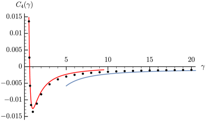
FIG. 1: Plot of the coefficient $C_{4}$. The dots represent numerically exact values and the curves are obtained from the analytical results (Local Properties of the Rapidity Distribution in the Lieb–Liniger Model) and (Local Properties of the Rapidity Distribution in the Lieb–Liniger Model).

The limiting cases of $C_{4}$ can be understood in terms of simple physics. At weak interactions, the free energy of the system can be calculated by studying the statistical mechanics of bosonic quasiparticles with Bogoliubov spectrum. It yields the result (Local Properties of the Rapidity Distribution in the Lieb–Liniger Model) taken at the leading order De Rosi et al. (2019). Interestingly, Bogoliubov spectrum is not the correct form of the quasiparticle spectrum at smallest momenta, as it is replaced by the fermionic one Pustilnik and Matveev (2014); Petković and Ristivojevic (2018). However, such picture with bosonic quasiparticles is sufficient in order to reproduce the leading-order coefficient in front of $\tau^{4}$ power in the free energy . In the limiting case of strong interactions, by calculating the free energy of the gas of noninteracting fermions we recovered the leading order term in Eq. (Local Properties of the Rapidity Distribution in the Lieb–Liniger Model). Nevertheless, the expression (Local Properties of the Rapidity Distribution in the Lieb–Liniger Model) applies at any interaction. In Fig. 2 we show the dimensionless free energy per particle for different values of the temperature.

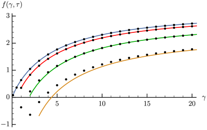
FIG. 2: The dimensionless free energy per particle $f(\gamma,\tau)$ obtained from the analytical expression (21) is represented by the curves and the one obtained by numerically solving the Yang–Yang equation is shown by the dots. Four distinct values of $\tau$ are considered: $0.1$, $1$, $2$, and $3$. For a fixed value of $\gamma$, the function $f(\gamma,\tau)$ decreases when $\tau$ increases. This is expected as the entropy of the system increases with the temperature. The agreement between Eq. (21) and numerically exact values is perfect for $\tau$ smaller than 1 and $\gamma$ larger than $\tau$. On the resolution of the plot, the curve for $\tau=0$ would be indistinguishable from the plotted one for $\tau=0.1$.

The derivation of Eq. (21).—The thermodynamic properties of the system can be calculated exactly. They follow from the Yang–Yang equation Yang and Yang (1969)

$$\bar{\mathcal{E}}(k)=-\bar{\mu}+\frac{\hbar^{2}k^{2}}{2m}+\frac{1}{2\pi}\int_{-\infty}^{+\infty}dq\;\!\frac{\theta(q-k)\bar{\mathcal{E}}^{\prime}(q)}{1+e^{\bar{\mathcal{E}}(q)/T}}.$$ (25)

The solution $\bar{\mathcal{E}}(k)$ of Eq. (25) depends on the chemical potential $\bar{\mu}$ and the temperature $T$. It enables one to calculate the pressure of the system in the grand-canonical ensemble,

$$\bar{P}=\frac{1}{2\pi}\int_{-\infty}^{+\infty}dq\;\!\frac{q\;\!\bar{\mathcal{E}}^{\prime}(q)}{1+e^{\bar{\mathcal{E}}(q)/T}}.$$ (26)

The free energy of the system in the canonical ensemble is then given by $F=-\bar{P}L+\bar{\mu}N$, where $L$ is the system size.

From a basic analysis it follows that $\bar{\mathcal{E}}(k)$ is an even real function, monotonically increasing for $k>0$. It thus nullifies at some $k=\bar{Q}$,

$$\bar{\mathcal{E}}(\bar{Q})=0.$$ (27)

In the zero-temperature limit, the denominator in the integral of Eq. (25) makes the boundary of integration finite, $Q$, corresponding the the Fermi rapidity. At low temperatures, Eq. (25) admits a series expansion in even powers of temperature, $\bar{\mathcal{E}}(k)=\mathcal{E}(k)+T^{2}\mathcal{E}_{2}(k)+T^{4}\mathcal{E}_{4}(k)+\mathcal{O}(T^{6})$. Similarly, we have $\bar{Q}=Q+T^{2}Q_{2}+T^{4}Q_{4}+\mathcal{O}(T^{6})$. Performing the Sommerfeld-like expansion of Eq. (25) we obtain a hierarchy of equations for $\mathcal{E}(k)$, $\mathcal{E}_{2}(k)$, and $\mathcal{E}_{4}(k)$. They should be combined with Eq. (27) as well as three equations obtained by successfully differentiating Eq. (1) with respect to $Q$. There we account for the derivatives $\mathcal{E}^{(j)}(Q)$ and $\mathcal{E}_{2}^{(j)}(Q)$. The latter follow from

$$\mathcal{E}_{2}(k)=-\frac{\pi^{2}m}{3\hbar^{2}n}\rho^{(0,1)}(k,Q),$$ (28)

and the former can be calculated using the formalism developed in Ref. Ristivojevic (2022). The final results are

$$\mathcal{E}^{\prime}(Q)={}\frac{\hbar^{2}n}{2m}\frac{1}{\rho(Q,Q)},$$ (29)

$$\mathcal{E}^{(j+2)}(Q)={}\frac{2\pi\hbar^{2}\rho^{(j,0)}(Q,Q)}{m}-\frac{\hbar^{2}n\rho^{(j,1)}(Q,Q)}{2m\rho^{2}(Q,Q)},$$ (30)

for $j=0,1,2,\cdots$. Eventually, using Eq. (26) we can express the pressure as $\bar{P}=P+T^{2}P_{2}+T^{4}P_{4}+\mathcal{O}(T^{6})$, where $P=\bar{\mu}n-E_{0}/L$, $P_{2}=\pi/6\hbar v$. The expression for $P_{4}$ is significantly more complicated, see Appendix. It can be expressed in terms of $\rho(Q,Q)$ and its total derivatives, $\rho^{(1,0)}(Q,Q)$, and $\rho^{(2,0)}(Q,Q)$.

The pressure enables us to obtain the density $\bar{n}$ in the grand-canonical ensemble, $\bar{n}=({\partial\bar{P}}/{\partial\bar{\mu}})_{T}$. It depends on the temperature, $\bar{n}=n+T^{2}n_{2}+\cdots$, with $n_{2}=(1/\hbar v)(\partial P_{2}/\partial Q)$. Here we have used $\partial\bar{\mu}/\partial Q=\hbar v$. In the final step we should transform the results to the canonical ensemble. There, $\bar{n}=n=N/L$ is fixed and $\bar{\mu}$ depends on the temperature, $\bar{\mu}=\mu+T^{2}\mu_{2}+\cdots$. Since $\bar{\mu}$, $n$, and $T$ are mutually related (the density is an integral of a function that depends on $\bar{\mu}$ and $T$ in the thermodynamic Bethe ansatz Yang and Yang (1969)) we use the exact relation

$$\left(\frac{\partial\bar{\mu}}{\partial T}\right)_{n}{\left(\frac{\partial n}{\partial\bar{\mu}}\right)_{T}}=-\left(\frac{\partial n}{\partial T}\right)_{\bar{\mu}}.$$ (31)

It enables us to find $\mu_{2}=-\pi\hbar vn_{2}/K$. Substituting the low-temperature forms of $\bar{P}$ and $\bar{\mu}$, the free energy density takes the form

$$\frac{F}{L}=\mu n-P-P_{2}T^{2}-\left(P_{4}+\frac{n_{2}\mu_{2}}{2}\right)T^{4}+\mathcal{O}(T^{6}).$$ (32)

In order to obtain Eq. (32) we have used the relations $P^{\prime}(\mu)=n$, ${P}_{2}^{\prime}(\mu)=n_{2}$, and $P^{\prime\prime}(\mu)={K}/{\pi\hbar v}$, where the prime denotes the derivative with respect to $\bar{\mu}$ at $\bar{\mu}=\mu$. Note that the leading temperature corrections to $\bar{n}$ and $\bar{\mu}$ are sufficient to find the term proportional to $T^{4}$ in the free energy. Substituting $\mu_{2}$ and $n_{2}$, the final result for $f(\gamma,\tau)=F/N\epsilon$ is given by Eq. (21) with

$$C_{4}{} =-\frac{64\pi^{6}\rho^{8}}{45}\biggl{[}1+\frac{3n\rho^{(1,0)}}{8\pi\rho^{3}}-\frac{3n^{2}\dot{\rho}\rho^{(1,0)}}{32\pi^{2}\rho^{6}}-\frac{5n^{2}\rho^{(2,0)}}{128\pi^{2}\rho^{5}}$$

$$+\frac{5n^{2}(\rho^{(1,0)})^{2}}{256\pi^{2}\rho^{6}}-\frac{n\dot{\rho}}{2\pi\rho^{3}}-\frac{n^{2}\dot{\rho}^{2}}{256\pi^{2}\rho^{6}}+\frac{17n^{2}\ddot{\rho}}{512\pi^{2}\rho^{5}}\biggr{]}.$$ (33)

Here we have suppressed the arguments $(Q,Q)$ after $\rho$ and its derivatives. Using Eqs. (12)–(15) we can express $\rho^{(1,0)}(Q,Q)$ and $\rho^{(2,0)}(Q,Q)$ in terms of $K_{1}$. Then Eq. (Local Properties of the Rapidity Distribution in the Lieb–Liniger Model) becomes the result (Local Properties of the Rapidity Distribution in the Lieb–Liniger Model).

Discussion.—Once the free energy is evaluated, the calculation of other thermodynamic parameters in the canonical ensemble is simple. The chemical potential is given by $\bar{\mu}=(1/L){\partial F}/{\partial n}$ and the pressure is $\bar{P}=\bar{\mu}n-n\epsilon f(\gamma,\tau)$, the entropy is $S=-{\partial F}/{\partial T}$, and the internal energy is $U=F+TS$. Finally, the specific heat is given by $C={\partial U}/{\partial T}$. After evaluation it reads

$$C=N\left(\frac{K}{6}\tau-12C_{4}\tau^{3}+\mathcal{O}(\tau^{5})\right).$$ (34)

Therefore, $C_{4}$ controls the leading correction term.

Until now we have been focused on the Lieb–Liniger model. However, many of the obtained results are valid beyond it. Equation (1) supplemented by a proper scattering phase shift also describes other Galilean-invariant integrable models. In the case of nonsingular phase shifts, the density of quasimomenta is an analytic function and Eq. (2) will remain valid Petković and Ristivojevic (2018); Ristivojevic (2023). Therefore Eqs. (4) and (6) are unaffected. Moreover, Eq. (21) is a general form of the dimensionless free energy per particle with $C_{4}$ given by Eq. (Local Properties of the Rapidity Distribution in the Lieb–Liniger Model). A notable example of Galilean-invariant integrable models with noncontact interaction is the hyperbolic Calogero–Sutherland model. It is characterized by the interaction potential $V(x)=\hbar^{2}\lambda(\lambda-1)\kappa^{2}/m\sinh^{2}(\kappa x)$ Sutherland (2004). However, finding explicit results for the latter model is beyond the scope of this work as we are not aware of analytical expression for the Luttinger liquid parameter $K$ in terms of the microscopic parameters of the model.

The family of parameters $K_{j}$, see Eq. (11), is important well-beyond the Yang–Yang thermodynamics. One example is the low-momentum spectrum of elementary excitations Petković and Ristivojevic (2018). Another one is the dynamical correlation function at low temperatures Eßler et al. (1998). The present work shows that $K_{j}$ parameters are not independent, but are hierarchically ordered, satisfying certain differential equations. We have shown how they can be explicitly solved in the case of the Bose gas with contact repulsion.

In conclusion, we have developed the formalism that enables the treatment of thermodynamics of Galilean-invariant integrable models at low temperatures at arbitrary interactions. The obtained results are beyond the ones obtained using conformal field theory. The leading correction to the old result for the free energy is accounted by Eqs. (21) and (Local Properties of the Rapidity Distribution in the Lieb–Liniger Model). It can be expressed in terms of the Luttinger liquid parameter $K$ and newly introduced dimensionless parameters $K_{1}$ and $K_{2}$, see Eqs. (12) and (13). For the special case of the Lieb–Liniger model, due to the connection (15), only $K$ and $K_{1}$ are involved, see Eq. (Local Properties of the Rapidity Distribution in the Lieb–Liniger Model). Moreover, for the latter model we have explicitly calculated the corresponding series expansions at weak and strong interactions. Our approach can be extended to account for further terms in the free energy.

Work at Laboratoire de Physique Théorique was supported in part by the EUR grant NanoX ANR-17-EURE-0009 in the framework of the “Programme des Investissements d’Avenir”.

End matter

Appendix A: Differential equations for $\rho^{(3,0)}(Q,Q)$ and $\rho^{(4,0)}(Q,Q)$.—In order to illustrate the general procedure of obtaining the derivatives of $\rho^{(j,0)}(Q,Q)$ described in the main text, here we report the differential equations for the cases $j=3$ and $j=4$. These quantities would be important, for example, to obtain higher order corrections in the free energy at low temperatures. The final results are

$$\frac{d}{dQ} \left(\frac{\rho^{(3,0)}(Q,Q)}{\rho(Q,Q)}\right)=\frac{R^{2}(Q)}{2}+\frac{1}{4}\frac{d^{2}R(Q)}{dQ^{2}}$$

$$+\frac{1}{2}\frac{dR(Q)}{dQ}\frac{\rho^{(1,0)}(Q,Q)}{\rho(Q,Q)}+R(Q)\frac{\rho^{(2,0)}(Q,Q)}{\rho(Q,Q)}$$ (A1)

and

$$\frac{d}{dQ} \left(\frac{\rho^{(4,0)}(Q,Q)}{\rho(Q,Q)}\right)=\frac{1}{8}\frac{d^{3}R(Q)}{dQ^{3}}+\frac{1}{2}\frac{dR^{2}(Q)}{dQ}$$

$$+\left(\frac{R^{2}(Q)}{2}+\frac{1}{4}\frac{d^{2}R(Q)}{dQ^{2}}\right)\frac{\rho^{(1,0)}(Q,Q)}{\rho(Q,Q)}$$

$$+\frac{1}{2}\frac{dR(Q)}{dQ}\frac{\rho^{(2,0)}(Q,Q)}{\rho(Q,Q)}+R(Q)\frac{\rho^{(3,0)}(Q,Q)}{\rho(Q,Q)}.$$ (A2)

We have also derived the equations for $\rho^{(5,0)}(Q,Q)$ and $\rho^{(6,0)}(Q,Q)$. They involve an increasingly larger number of terms and are thus not reported here.

Appendix B: Subleading corrections to the pressure and the free energy.—The subleading temperature correction of the pressure in the grand-canonical ensemble is given by

$$P_{4}=\frac{224\pi^{6}m^{3}\rho^{8}}{15\hbar^{6}n^{5}}\biggl{[}1-\frac{13n\dot{\rho}}{21\pi\rho^{3}}+\frac{19n^{2}\dot{\rho}^{2}}{336\pi^{2}\rho^{6}}+\frac{17n^{2}\ddot{\rho}}{672\pi^{2}\rho^{5}}$$

$$+\frac{2n\rho^{(1,0)}}{7\pi\rho^{3}}-\frac{n^{2}\dot{\rho}\rho^{(1,0)}}{14\pi^{2}\rho^{6}}+\frac{5n^{2}(\rho^{(1,0)})^{2}}{336\pi^{2}\rho^{6}}-\frac{5n^{2}\rho^{(2,0)}}{168\pi^{2}\rho^{5}}\biggr{]}.$$ (B1)

As in the main text, we have suppressed the arguments $(Q,Q)$ of $\rho$ and its derivatives. Equation (Local Properties of the Rapidity Distribution in the Lieb–Liniger Model) arises from the Sommerfeld-like expansion of the pressure $\bar{P}$ and the pseudoenergy $\bar{\mathcal{E}}(k)$ combined with the relation of the latter with the ground-state distribution $\rho(k,Q)$ and its derivatives.

In the second temperature correction of the free energy (32), two terms appear. One is $P_{4}$ given by Eq. (Local Properties of the Rapidity Distribution in the Lieb–Liniger Model) and the other is a combination $\mu_{2}n_{2}$. The latter is related to the derivative of the sound velocity $v$ with respect to the Fermi rapidity $Q$. It can also be expressed in terms of the derivative of $v$ with respect to the chemical potential (at zero temperature). We have

$$\mu_{2}n_{2}=-\frac{\pi^{3}}{36\hbar^{3}Kv}\left(\frac{\partial}{\partial Q}\frac{1}{v}\right)^{2}=-\frac{m^{3}K^{2}}{36\hbar^{4}n^{3}}\left(\frac{dv}{d\mu}\right)^{2}.$$ (B2)

Using $mvK=\pi\hbar n$ and $K=4\pi^{2}\rho(Q,Q)^{2}$, we obtain

$$\frac{dv}{d\mu}=\frac{4\pi\rho^{2}}{\hbar n}-\frac{2\dot{\rho}}{\hbar\rho}.$$ (B3)

Thus both contributions in term proportional to $T^{4}$ of the free energy can be expressed in terms $\rho(Q,Q)$ and its derivatives.

References

- Lieb and Liniger (1963) E. H. Lieb and W. Liniger, “Exact Analysis of an Interacting Bose Gas. I. The General Solution and the Ground State,” Phys. Rev. 130, 1605 (1963).
- Korepin et al. (1993) V. E. Korepin, N. M. Bogoliubov, and A. G. Izergin, Quantum Inverse Scattering Method and Correlation Functions (Cambridge University Press, Cambridge, England, 1993).
- Gaudin (2014) M. Gaudin, The Bethe Wavefunction (Cambridge University Press, Cambridge, England, 2014).
- Paredes et al. (2004) B. Paredes, A. Widera, V. Murg, O. Mandel, S. Fölling, I. Cirac, G. V. Shlyapnikov, T. W. Hänsch, and I. Bloch, “Tonks–Girardeau gas of ultracold atoms in an optical lattice,” Nature 429, 277 (2004).
- Kinoshita et al. (2004) T. Kinoshita, T. Wenger, and D. S. Weiss, “Observation of a One-Dimensional Tonks-Girardeau Gas,” Science 305, 1125 (2004).
- Cheianov et al. (2006) V. V. Cheianov, H. Smith, and M. B. Zvonarev, “Exact results for three-body correlations in a degenerate one-dimensional Bose gas,” Phys. Rev. A 73, 051604(R) (2006).
- Pozsgay (2011) B. Pozsgay, “Local correlations in the 1D Bose gas from a scaling limit of the XXZ chain,” J. Stat. Mech. 2011, P11017 (2011).
- Bastianello et al. (2018) A. Bastianello, L. Piroli, and P. Calabrese, “Exact Local Correlations and Full Counting Statistics for Arbitrary States of the One-Dimensional Interacting Bose Gas,” Phys. Rev. Lett. 120, 190601 (2018).
- Ristivojevic (2022) Z. Ristivojevic, “Method of difference-differential equations for some Bethe-ansatz-solvable models,” Phys. Rev. A 106, 062216 (2022).
- Shashi et al. (2012) A. Shashi, M. Panfil, J.-S. Caux, and A. Imambekov, “Exact prefactors in static and dynamic correlation functions of one-dimensional quantum integrable models: Applications to the Calogero–Sutherland, Lieb–Liniger, and XXZ models,” Phys. Rev. B 85, 155136 (2012).
- Kitanine et al. (2012) N. Kitanine, K. K. Kozlowski, J. M. Maillet, N. A. Slavnov, and V. Terras, “Form factor approach to dynamical correlation functions in critical models,” J. Stat. Mech. 2012, P09001 (2012).
- De Nardis and Panfil (2016) J. De Nardis and M. Panfil, “Exact correlations in the Lieb–Liniger model and detailed balance out-of-equilibrium,” SciPost Physics 1, 015 (2016).
- Caux and Essler (2013) J.-S. Caux and F. H. L. Essler, “Time Evolution of Local Observables After Quenching to an Integrable Model,” Phys. Rev. Lett. 110, 257203 (2013).
- Caux (2016) J.-S. Caux, “The Quench Action,” J. Stat. Mech. 2016, 064006 (2016).
- Castro-Alvaredo et al. (2016) O. A. Castro-Alvaredo, B. Doyon, and T. Yoshimura, “Emergent Hydrodynamics in Integrable Quantum Systems Out of Equilibrium,” Phys. Rev. X 6, 041065 (2016).
- Bertini et al. (2016) B. Bertini, M. Collura, J. De Nardis, and M. Fagotti, “Transport in Out-of-Equilibrium XXZ Chains: Exact Profiles of Charges and Currents,” Phys. Rev. Lett. 117, 207201 (2016).
- Haldane (1981) F. D. M. Haldane, “Effective Harmonic-Fluid Approach to Low-Energy Properties of One-Dimensional Quantum Fluids,” Phys. Rev. Lett. 47, 1840 (1981).
- Sutherland (2004) B. Sutherland, Beautiful models (World Scientific, Singapore, 2004).
- Wilson et al. (2020) J. M. Wilson, N. Malvania, Y. Le, Y. Zhang, M. Rigol, and D. S. Weiss, “Observation of dynamical fermionization,” Science 367, 1461 (2020).
- Dubois et al. (2024) L. Dubois, G. Thémèze, F. Nogrette, J. Dubail, and I. Bouchoule, “Probing the Local Rapidity Distribution of a One-Dimensional Bose Gas,” Phys. Rev. Lett. 133, 113402 (2024).
- Yang and Yang (1969) C. N. Yang and C. P. Yang, “Thermodynamics of a One‐Dimensional System of Bosons with Repulsive Delta‐Function Interaction,” J. Math. Phys. 10, 1115 (1969).
- van Amerongen et al. (2008) A. H. van Amerongen, J. J. P. van Es, P. Wicke, K. V. Kheruntsyan, and N. J. van Druten, “Yang-Yang Thermodynamics on an Atom Chip,” Phys. Rev. Lett. 100, 090402 (2008).
- Jacqmin et al. (2011) T. Jacqmin, J. Armijo, T. Berrada, K. V. Kheruntsyan, and I. Bouchoule, “Sub-Poissonian Fluctuations in a 1D Bose Gas: From the Quantum Quasicondensate to the Strongly Interacting Regime,” Phys. Rev. Lett. 106, 230405 (2011).
- Vogler et al. (2013) A. Vogler, R. Labouvie, F. Stubenrauch, G. Barontini, V. Guarrera, and H. Ott, “Thermodynamics of strongly correlated one-dimensional Bose gases,” Phys. Rev. A 88, 031603 (2013).
- Affleck (1986) I. Affleck, “Universal term in the free energy at a critical point and the conformal anomaly,” Phys. Rev. Lett. 56, 746 (1986).
- Blöte et al. (1986) H. W. J. Blöte, J. L. Cardy, and M. P. Nightingale, “Conformal invariance, the central charge, and universal finite-size amplitudes at criticality,” Phys. Rev. Lett. 56, 742 (1986).
- Guan and Batchelor (2011) X.-W. Guan and M. T. Batchelor, “Polylogs, thermodynamics and scaling functions of one-dimensional quantum many-body systems,” J. Phys. A: Math. Theor. 44, 102001 (2011).
- Kerr et al. (2024) M. L. Kerr, G. De Rosi, and K. Kheruntsyan, “Analytic thermodynamic properties of the Lieb–Liniger gas,” SciPost Phys. Core 7, 047 (2024).
- De Rosi et al. (2019) G. De Rosi, P. Massignan, M. Lewenstein, and G. E. Astrakharchik, “Beyond-Luttinger-liquid thermodynamics of a one-dimensional Bose gas with repulsive contact interactions,” Phys. Rev. Research 1, 033083 (2019).
- Petković and Ristivojevic (2018) A. Petković and Z. Ristivojevic, “Spectrum of Elementary Excitations in Galilean-Invariant Integrable Models,” Phys. Rev. Lett. 120, 165302 (2018).
- Ristivojevic (2023) Z. Ristivojevic, “Exact Results for the Moments of the Rapidity Distribution in Galilean-Invariant Integrable Models,” Phys. Rev. Lett. 130, 020401 (2023).
- Popov (1977) V. N. Popov, “Theory of one-dimensional Bose gas with point interaction,” Theor. Math. Phys. 30, 222 (1977).
- Pustilnik and Matveev (2014) M. Pustilnik and K. A. Matveev, “Low-energy excitations of a one-dimensional Bose gas with weak contact repulsion,” Phys. Rev. B 89, 100504(R) (2014).
- Pustilnik and Matveev (2015) M. Pustilnik and K. A. Matveev, “Fate of classical solitons in one-dimensional quantum systems,” Phys. Rev. B 92, 195146 (2015).
-
Note (1)
Interestingly, the numbers in Eq. (18b)
are identical to the coefficients appearing in Stirling’s series for the
Gamma function, , written in the form
- Ristivojevic (2019) Z. Ristivojevic, “Conjectures about the ground-state energy of the Lieb-Liniger model at weak repulsion,” Phys. Rev. B 100, 081110(R) (2019).
- Ristivojevic (2014) Z. Ristivojevic, “Excitation Spectrum of the Lieb–Liniger Model,” Phys. Rev. Lett. 113, 015301 (2014).
- Note (2) Recall that the ground-state energy of the Lieb–Liniger model at the leading and the subleading order is correctly reproduced by the same approach with Bogoliubov quasiparticles Lieb and Liniger (1963).
- Eßler et al. (1998) F. Eßler, V. Korepin, and F. Latrémolière, “Temperature corrections to conformal field theory,” Eur. Phys. J. B 5, 559 (1998).