Generalized local polynomial reproductions

Abstract.

We present a general framework, treating Lipschitz domains in Riemannian manifolds, that provides conditions guaranteeing the existence of norming sets and generalized local polynomial reproductions—a powerful tool used in the analysis of various mesh-free methods and a mesh-free method in its own right. As a key application, we prove the existence of smooth local polynomial reproductions on compact subsets of algebraic manifolds in $\mathbb{R}^{n}$ with Lipschitz boundary. These results are then applied to derive new findings on the existence, stability, regularity, locality, and approximation properties of shape functions for a coordinate-free moving least squares approximation method on algebraic manifolds, which operates directly on point clouds without requiring tangent plane approximations.

1. Introduction

Let $\mathbb{M}$ be a smooth compact $d$-dimensional Riemannian manifold without boundary. In this article, we provide the existence of a smooth generalization of the local polynomial reproduction on $\mathbb{M}$. Specifically, for certain bounded regions $\Omega\subset\mathbb{M}$, and function spaces $\varPi\subset C^{1}(\mathbb{M})$ (which satisfy Assumptions 1 and 2 described below) and for sampled finite subsets $\Xi\subset\Omega$ that are sufficiently dense, we prove existence of a map $a:\Xi\times\Omega\to\mathbb{R}$ which satisfies the following properties

• $\varPi$-reproduction: $(\forall p\in\varPi)(\forall z\in\Omega)$ $\sum_{\xi\in\Xi}a(\xi,z)p(\xi)=p(z)$

• stability: $\sup_{z\in\Omega}\sum_{\xi\in\Xi}|a(\xi,z)|<2$

• locality: $a(\xi,z)=0$ unless $\xi$ is near to $z$

• regularity: if $\varPi\subset C^{\infty}(\mathbb{M})$, then each $a(\xi,\cdot)\in C^{\infty}(\mathbb{M})$.

As a consequence of this general result, we demonstrate the existence of local polynomial reproductions (i.e., $\varPi=\mathcal{P}_{m}(\mathbb{R}^{N})$, polynomials of fixed degree at most $m$) on Lipschitz domains in algebraic manifolds $\mathbb{M}$ in $\mathbb{R}^{N}$.

As in the archetypal Euclidean case, considered in [22] and [36], which forms a model for our results, the key to the construction is to establish that $\Xi$ is a norming set (sometimes called an admissible mesh) for the norm on $C(\Omega)$. In short, this means that the sampling operator $S:C(\Omega)\to\ell_{\infty}(\Xi):f\mapsto f|_{\Xi}$ is bounded below by a fixed constant, independent of the cardinality of $\Xi$.

In the Euclidean setting, this relies heavily on Markov’s inequality

$$\|p^{\prime}\|_{C([0,T])}\leq\frac{2m^{2}}{T}\|p\|_{C([0,T])}$$

for algebraic polynomials $p\in\mathcal{P}_{m}(\mathbb{R})$. For spherical harmonics on $\mathbb{S}^{d}$, Markov’s inequality can be replaced by Videnskii’s inequality [35, Eqn. (2)].

Although Markov inequalities exist in a variety of exotic contexts, particularly for smooth algebraic varieties in [6, 5] and for boundaries of convex sets in [24], they are often global in nature, and unsuitable for adapting the Euclidean argument developed in [22] and [36]. We make a subtle but significant modification to the established Euclidean machinery to accommodate work on Riemannian manifolds. This involves Markov-like covariant derivative estimates in conjunction with a doubling estimate. These have been established for algebraic polynomials on algebraic manifolds in [4] and [13], and likely exist for other systems of elementary functions on manifolds (see, for instance, Laplacian eigenfunctions in [11]).

1.1. Applications of stable polynomial reproductions

Local polynomial reproductions and related constructions on spheres provide a powerful tool for providing error estimates in scattered data approximation. They have been used to obtain sampling inequalities, first introduced by Madych and Potter [28], but more recently considered in [31, 30]. They are also crucial to a number of estimates in kernel and RBF approximation. Wu and Schaback, in [38], use local polynomial reproductions to estimate the power function $P_{X}$ for RBF interpolation, which measures the norm of the interpolation error functional $f\mapsto f(x)-I_{X}f(x)$ over a reproducing kernel Hilbert space associated with the RBF. DeVore and Ron, in [10], use local polynomial reproductions to get kernel approximation results on $\mathbb{R}^{d}$. Videnski’i’s inequality has been used to provide a local spherical harmonic reproduction used in [20] and on SO(3) in [18].

1.2. Moving Least Squares

A specific motivating application for the theory presented in this article is moving least squares (MLS) approximation on algebraic manifolds. MLS has origins in work of Shepard [32] and was studied in the 1980s by Lancaster, Farwig, Salkauskas [25, 12] and others. For a set of points $\Xi$ in a domain $\Omega\subset\mathbb{R}^{d}$, an MLS approximant for the data $\boldsymbol{\mathbf{y}}=(y_{\xi})_{\xi\in\Xi}\subset\mathbb{R}$ takes the form

(1) $$\operatorname{MLS}_{\Xi,\boldsymbol{\mathbf{y}}}(\zeta):=p_{\zeta}^{*}(\zeta),\text{ where }p_{\zeta}^{*}:=\arg\min_{p\in\mathcal{P}_{m}(\mathbb{R}^{d})}\sum_{\xi\in\Xi}\left(p(\xi)-y_{\xi}\right)^{2}\mathcal{W}(\xi,\zeta),$$

$\zeta\in\Omega$ is a given point and $\mathcal{W}:\Omega\times\Omega\to[0,\infty)$ is a given weight function. Approximation theoretic results for $\Omega\subset\mathbb{R}^{d}$ were given, for example, in [26] and [36].

Our goal is to develop a MLS technique for algebraic manifolds $\Omega\subset\mathbb{M}$ that does not use intrinsic coordinates to $\Omega$ (i.e., coordinate-free) or tangent plane approximations. We then follow a similar approach of [36], which explicitly uses the kinds of local polynomial reproductions we develop here, to analyze the approximation properties of the method.

MLS methods are used widely as mesh-free techniques for solving partial differential equations (PDES) (e.g.,[3, 27, 2, 29, 34]) and have been extended to spherical regions in [37, 21]. Recent works, such as [23, 33], have also extended MLS to problems on embedded manifolds. However, unlike to our coordinate-free approach, these methods address the basic problem (1) by projecting points onto tangent spaces.

1.3. Outline

In the next section, we introduce Assumptions 1 and 2 which guarantee a norming set property, among other useful properties; this is a standard method for generating local polynomial reproductions, which we consider in section 4 to generate a local $\varPi$-reproduction. Unlike established constructions as in [36], we investigate the smoothness of the basic functions, in addition to their stability and locality. This follows the argument recently developed in the Euclidean setting in [17].

In section 5 we consider a constructive method for obtaining local $\varPi$-reproductions based on MLS approximation. This has the advantage that derivatives of the local $\varPi$-reproduction reproduce derivatives of functions in $\varPi$. We prove stability, smoothness and locality of this methodology.

Section 6 treats the concrete application of local (restricted) polynomial reproductions on algebraic manifolds, which employs analytic results from [13]. Numerical experiments for this setup are considered in section 7.

2. Geometric Background

2.1. Background

Throughout this paper, we assume $\mathbb{M}$ is a connected, $d$-dimensional Riemannian manifold. We denote by $T\mathbb{M}$ the tangent bundle of $\mathbb{M}$, and by $T^{k_{1}}_{k_{2}}\mathbb{M}$ the vector bundle of tensors with contravariant rank $k_{1}$ and covariant rank $k_{2}$ (in particular, $T^{1}_{0}\mathbb{M}=T\mathbb{M}$ is the tangent bundle and $T^{0}_{1}\mathbb{M}=T^{*}\mathbb{M}$ is the cotangent bundle). We will denote the fiber at $x\in\mathbb{M}$ by $T^{k_{1}}_{k_{2}}\mathbb{M}_{x}$. In this article, we will be concerned primarily with covariant tensors.

The fact that $\mathbb{M}$ is a Riemannian manifold means that on each tangent space $T\mathbb{M}_{x}$ there is an inner product. This extends by duality to each fiber $T^{k_{1}}_{k_{2}}\mathbb{M}_{x}$ of the tensor bundle: for instance, for a covariant tensor $S\in T^{0}_{k}\mathbb{M}_{x}$, we have

(2) $$\|S\|_{T^{0}_{k}\mathbb{M}_{x}}=\max_{(V_{1},\dots,V_{k})\in(T\mathbb{M}_{x})^{k}\setminus\{0\}}\frac{|S(V_{1},\dots,V_{k})|}{\|V_{1}\|_{T\mathbb{M}_{x}}\dots\|V_{k}\|_{T\mathbb{M}_{x}}}.$$

2.1.1. Tensor fields

For a chart $(U,\phi)$ for $\mathbb{M}$ we get the usual vector fields $\frac{\partial}{\partial x^{j}}$ and forms $dx_{j}$ ($1\leq j\leq d$), which act as local bases for $T\mathbb{M}$ and $T^{*}\mathbb{M}$ over $U$.

These can be used to generate bases for tensor fields (i.e., sections of tensor bundles). In particular, for a covariant tensor field $T:\mathbb{M}\to T^{0}_{k}\mathbb{M}$, we have basis elements $dx_{\hat{\imath}}:=dx_{i_{1}}\cdots dx_{i_{k}}$ for $\hat{\imath}=(i_{1},\dots,i_{k})\in\{1,\dots,d\}^{k}$, which allow us to write $T$ in coordinates as $T(x)=\sum_{\hat{\imath}\in\{1,\dots,d\}^{k}}(T(x))_{\hat{\imath}}dx_{\hat{\imath}}$.

Of particular interest is Riemannian metric tensor $g:\mathbb{M}\to T^{0}_{2}\mathbb{M}$, written in coordinates over $U$ as $g(x)=\sum_{i,j\leq d}g_{ij}(x)dx_{i}dx_{j}$. Similarly, the volume element on $\mathbb{M}$ is $\mathrm{d}\mu=\sqrt{\det(g_{ij})}dx_{1}\dots dx_{d}$.

At a point $x\in U$, the tangent space $T\mathbb{M}_{x}$ has inner product $\langle T,S\rangle_{T\mathbb{M}_{x}}=\sum g_{ij}T_{i}S_{j}$, where $T=\sum_{i=1}^{d}T_{i}\frac{\partial}{\partial x^{i}}$ and $S=\sum_{j=1}^{d}S_{j}\frac{\partial}{\partial x^{j}}$. The inner product on $T^{0}_{k}\mathbb{M}_{x}$ obtained from (2) can be expressed in coordinates as

$$\langle T,S\rangle_{T^{0}_{k}\mathbb{M}_{x}}=\sum_{\hat{\imath},\hat{\jmath}}g^{i_{1}j_{1}}(x)\cdots g^{i_{k}j_{k}}(x)T_{\hat{\imath}}S_{\hat{\jmath}},$$

where $(g^{ij})$ is the matrix inverse of $(g_{ij})$, $T=\sum_{\hat{\imath}}(T)_{\hat{\imath}}dx_{\hat{\imath}}$. and $S=\sum_{\hat{\jmath}}(S)_{\hat{\jmath}}dx_{\hat{\jmath}}$ (see [15, Eqn. (2.1)]).

2.1.2. Geodesics and exponential map

We denote the Riemannian distance on $\mathbb{M}$ by $\operatorname{dist}:\mathbb{M}\times\mathbb{M}\to[0,\infty)$ or, to avoid confusion when multiple distances are in use, we use $\operatorname{dist}_{\mathbb{M}}$. Since $\mathbb{M}$ is connected, pairs of nearby points $x,y\in\mathbb{M}$ can be connected by a geodesic $\gamma:[a,b]\to\mathbb{M}$ with $\gamma(a)=x$, $\gamma(b)=y$ and $\operatorname{dist}(x,y)=\int_{a}^{b}\|\gamma^{\prime}(t)\|_{T\mathbb{M}_{\gamma(t)}}\mathrm{d}t$.

At every point $x\in\mathbb{M}$, the exponential map $\mathrm{Exp}_{x}:B(0,r_{x})\to{U}\subset\mathbb{M}$ is a smooth diffeomorphism defined on an open neighborhood of $0\in T_{x}\mathbb{M}$. It has the property that it preserves radial distances: for any $y=\mathrm{Exp}_{x}(v)\in{U}$, $\operatorname{dist}(x,y)=|0-v|$. In fact, the map $(x,v)\mapsto\mathrm{Exp}_{x}(v):\mathfrak{U}\to\mathbb{M}$ is defined and smooth on an open neighborhood $\mathfrak{U}$ of the zero section in $T\mathbb{M}$.

Consequently, for any compact set $\Omega\subset\mathbb{M}$, the quantity $r_{\Omega}=\min_{x\in\Omega}r_{x}$ is positive, and there exist constants $0<\Gamma_{1}\leq\Gamma_{2}$ such that for any $z\in\Omega$ and any $x,y\in B(0,\mathrm{r}_{\Omega})$, the metric equivalence

(3) $$\Gamma_{1}|x-y|\leq\operatorname{dist}(\mathrm{Exp}_{z}(x),\mathrm{Exp}_{z}(y))\leq\Gamma_{2}|x-y|$$

holds.

2.1.3. Covariant differentiation

The cotangent derivative $\nabla$ maps tensor fields of rank $(k_{1},k_{2})$ to tensor fields of rank $(k_{1},k_{2}+1)$. In particular, $\nabla^{k}$ maps functions to covariant tensor fields of rank $(0,k)$. We can use this to generate smoothness norms: for an open, bounded set $U\subset\mathbb{M}$,

$$\|f\|_{C^{k}(\overline{U})}:=\max_{j\leq k}\max_{x\in\overline{U}}\|\nabla^{j}f(x)\|_{T^{0}_{j}\mathbb{M}_{x}}.$$

If $\Omega\subset\mathbb{M}$ is compact, then [15, Lemma 3.2] ensures that there are uniform constants $C_{1},C_{2}{>0}$ so that the family of exponential maps $\{\mathrm{Exp}_{x}:B_{r}\to\mathbb{M}\mid x\in\Omega\}$ provides local metric equivalences: for any open set $U$ with $\overline{U}\subset B(0,{r_{\Omega}})$, we have

(4) $$C_{1}\|u\circ\mathrm{Exp}_{x}\|_{C^{k}(\overline{U})}\leq\|u\|_{C^{k}(\overline{\mathrm{Exp}_{x}(U)})}\leq C_{2}\|u\circ\mathrm{Exp}_{x}\|_{C^{k}(\overline{U})}.$$

This is an application of a more general result which treats metric equivalence of Sobolev norms. Although the full metric equivalence is not necessary for our purposes, another consequence is the following: for every $x\in\Omega$ and any $U\subset B(x,r_{\Omega})$,

(5) $$C_{1}\|u\circ\mathrm{Exp}_{x}\|_{L_{p}(U)}\leq\|u\|_{L_{p}(\mathrm{Exp}_{x}(U))}\leq C_{2}\|u\circ\mathrm{Exp}_{x}\|_{L_{p}(U)}.$$

For a metric space $\Omega$ and a set $\Xi\subset\Omega$, define the sampling operator $S_{\Xi}:f\mapsto f|_{\Xi}$ as a map from $C(\Omega)$ to $\ell_{\infty}(\Xi)$. We note that $\left\|S_{\Xi}\right\|\leq 1$. A norming set for a subspace $\Pi\subset C(\Omega)$ is a subset $\Xi\subset\Omega$ so that $S_{\Xi}$ is bounded below. Thus, finding a norming set $\Xi$ is equivalent to developing a Marcinkiewicz-type discretization for $p=\infty$, as considered in [8, Eqn. 1.2].

Such norming sets have been developed for scattered approximation on spheres in [22]. This has been expanded to treat subsets of $\mathbb{S}^{d}$ and Euclidean regions satisfying interior cone conditions in [36]. Out strategy resembles the latter, although the use of the doubling property (6) simplifies the argument.

Our goal in the next section is to prove a general norming set property: for balls $B_{1}\subset B_{2}$ and sufficiently dense $\Xi\subset\Omega$, the set $B_{2}\cap\Xi$ is a norming set for $(\varPi,\|\cdot\|_{C(B_{1}\cap\Omega)})$. In other words, when restricted to $\varPi$, the sampling operator

$$S_{\Xi}:(\varPi,\|\cdot\|_{C(B_{1}\cap\Omega)})\to\left(\mathbb{R}^{B_{2}\cap\Xi},\|\cdot\|_{\ell_{\infty}(B_{2}\cap\Xi)}\right),\quad p\mapsto p|_{B_{2}\cap\Xi}$$

is bounded below.

3. Local Markov property and preliminary results

3.1. Basic analytic and geometric assumptions

To prove the general result, we assume the following about the function space $\varPi$.

Assumption 1.

We assume that $\varPi\subset C^{1}(\mathbb{M})$ is a finite dimensional space of functions which satisfy a doubling condition and a Markov inequality. Namely, there exist constants $\mathfrak{D}$, $\mathfrak{M}$, and $r^{\sharp},>0$ so that for every $p\in\varPi$, $0<r<r^{\sharp},$ and $x_{0}\in\mathbb{M}$,

(6) $$\|p\|_{C(B(x_{0},2r))} \leq 2^{\mathfrak{D}}\|p\|_{C(B(x_{0},r))},$$

(7) $$\|\nabla p\|_{C(B(x_{0},r))} \leq\frac{{\mathfrak{M}}}{r}\|p\|_{C(B(x_{0},r))}.$$

We will discuss the applicability to restricted polynomials on algebraic manifolds later. For now, we point out that such results have been shown in [13] with constants ${\mathfrak{D}}$ and ${\mathfrak{M}}$ which depend on the polynomial degree.

In this section, we prove existence of a local $\varPi$-reproduction on compact subsets $\Omega\subset\mathbb{M}$ which satisfy an interior cone condition. To set up the definition, we define a basic Euclidean cone with parameters $r>0$, $0<\omega<\pi/2$ and $v\in\mathbb{S}^{d-1}$, as the set

$$C_{r,\omega,v}:=\{w\in\mathbb{R}^{d}\mid\|w\|\leq r\text{ and }v^{T}w\geq\cos(\omega)\}.$$

The interior cone condition for $\Omega\subset\mathbb{M}$ is similar to a Euclidean cone condition, but involves geodesic cones.

Assumption 2.

We assume that $\Omega\subset\mathbb{M}$ is compact, and that it satisfies an interior cone condition of radius $r^{\flat}>0$ and aperture $\omega<\pi/2$: for each point $z$ of $\Omega$, there is a direction $v\in\mathbb{S}^{d-1}$ so that $\mathrm{Exp}_{z}(C_{r^{\flat},\omega,v})\subset\Omega$.

We define the basic parameter, combining the injectivity radius $r_{\Omega}$, threshold distances for the Markov and doubling inequalities $r^{\sharp}$, and the cone parameter $r^{\flat}$:

$$r^{*}:=\min(r_{\Omega},r^{\sharp},r^{\flat}).$$

It follows that there exist constants $\alpha_{\Omega}\leq\beta_{\Omega}$ so that for any $x\in\Omega$ and $r\leq r^{*}$,

(8) $$\alpha_{\Omega}r^{d}\leq\mu(B(x,r)\cap\Omega)\leq\omega_{\Omega}r^{d}$$

(this is a direct consequence of (5),with $p=1$ and $u=\chi_{C_{r,\omega,v}}$).

We make use of the following result, which follows easily from [16, Lemma A.7] and shows that cones contain interior balls.

Lemma 3.1.

Suppose $\Omega\subset\mathbb{M}$ satisfies (3) and $\mathcal{C}=\mathrm{Exp}_{z}(C_{r^{\flat},\omega,v})\subset\Omega$. Then for $0<\rho<r^{\flat}/(1+\sin\omega)$, $r=\Gamma_{1}\rho\sin(\omega)$ and $\zeta=\mathrm{Exp}_{z}(\rho v)$, we have $\overline{B(\zeta,r)}\subset\mathcal{C}$.

Proof.

Note that $\rho\sin\omega\leq r^{\flat}-\rho$ and $r\leq\Gamma_{1}(r^{\flat}-\rho)$. Thus, if $\xi\in B(\zeta,r)$, then

$$\operatorname{dist}(z,\xi)<\rho+r\leq\Gamma_{1}r^{\flat}+(1-\Gamma_{1})\rho<r^{\flat}.$$

Hence $B(\zeta,r)\subset B(z,r^{\flat})$.

For $\xi\in B(z,r^{\flat})\setminus\mathcal{C}$, let $\xi=\mathrm{Exp}_{z}(tu)$ with $t<r^{\flat}$ and $u\in\mathbb{S}^{d-1}$. Then $tu\notin C_{r^{\flat},\omega,v}$, and hence $|tu-\rho v|>\rho\sin\omega$. Thus $\operatorname{dist}(\xi,\zeta)\geq\Gamma_{1}|tu-\rho v|>r$, so $\xi\notin\overline{B(\zeta,r)}$. ∎

For a point $x_{0}\in\Omega$, we can use Lemma 3.1 and the doubling property (6) to control the size of $\|p\|_{C(B(x_{0},R))}$ by using $\|p\|_{C(B(x_{0},R)\cap\Omega)}$.

Lemma 3.2.

Suppose $\varPi$ satisfies Assumption 1 and $\Omega\subset\mathbb{M}$ satisfies Assumption 2. Then for any $x_{0}\in\Omega$ and $R\leq r^{*}$,

$$\|p\|_{C(\overline{B(x_{0},R)})}\leq 2^{\mathfrak{D}}\left(\frac{2+\sin\omega}{\Gamma_{1}\sin\omega}\right)^{\mathfrak{D}}\|p\|_{C(\overline{B(x_{0},R)}\cap\Omega)}.$$

Proof.

Fix $p\in\varPi$. Find $z_{1}\in\overline{B(x_{0},R)}\cap\Omega$ and $z_{0}\in\overline{B(x_{0},R)}$ (possibly different than $z_{1}$) so that $|p(z_{1})|=\|p\|_{C(\overline{B(x_{0},R)}\cap\Omega)}$ and $|p(z_{0})|=\|p\|_{C(\overline{B(x_{0},R)})}$.

By assumption, there is a cone $\mathcal{C}=\mathrm{Exp}_{x_{0}}(C_{R,\omega,v})$ contained in $\overline{B(x_{0},R)}\cap\Omega$. Let $\rho:=R/(1+\sin(\omega))$, and note that for $\zeta:=\mathrm{Exp}_{x_{0}}(\rho v)$ and $r:=\Gamma_{1}\rho\sin\omega$, we have

$$\|p\|_{C(\overline{B(\zeta,r)})}\leq\|p\|_{C(\overline{B(x_{0},R)}\cap\Omega)}\leq|p(z_{1})|$$

since $\overline{B(\zeta,r)}$ is contained in $\mathcal{C}$ by Lemma 3.1.

At the same time, $\operatorname{dist}(z_{0},\zeta)\leq R+\rho$, so $z_{0}\in\overline{B(\zeta,R+\rho)}$. Find $j\in\mathbb{N}$ so that $2^{j-1}\Gamma_{1}{\sin\omega}\leq 2+\sin\omega<2^{j}\Gamma_{1}{\sin\omega}$, so $j$ depends only on $\Gamma_{1}$ and $\omega$. By the definition of $\rho$, we have $R+\rho<2^{j}\Gamma_{1}\rho\sin(\omega)$, so by applying the doubling inequality (6) $j$ times, we have that

$$|p(z)|\leq\|p\|_{C(\overline{B(\zeta,R+\rho)})}\leq 2^{j\mathfrak{D}}\|p\|_{C(\overline{B(\zeta,r)})}\leq 2^{\mathfrak{D}}\left(\frac{2+\sin\omega}{\Gamma_{1}\sin\omega}\right)^{\mathfrak{D}}|p(z_{1})|$$

and the lemma follows. ∎

3.2. A lower bound

Under assumptions 1 and 2, let us define

$$\kappa:={\mathfrak{M}}2^{2\mathfrak{D}}\left(\frac{2+\sin\omega}{\Gamma_{1}\sin\omega}\right)^{\mathfrak{D}}\frac{1+\Gamma_{1}\sin\omega}{\Gamma_{1}\sin\omega}$$

which will be used to describe the support radius of the norming set.

Lemma 3.3.

Suppose $\mathbb{M}$ is a Riemannian manifold, $\varPi\subset C^{1}(\mathbb{M})$ satisfies Assumption 1 and $\Omega\subset\mathbb{M}$ satisfies Assumption 2. Then for any $x_{0}\in\Omega$, $0<\epsilon<1$ and $R<r^{*}/(1+\epsilon)$ there is a ball $\tilde{B}:=\overline{B(\zeta,\frac{\epsilon R}{\kappa})}\subset\Omega\cap\overline{B(x_{0},(1+\epsilon)R)}$ so that for any $p\in\varPi$,

$$\min_{\xi\in\tilde{B}}|p(\xi)|\geq(1-\epsilon){\|p\|_{C(\overline{B(x_{0},R)}\cap\Omega)}}$$

holds.

Proof.

Without loss of generality, let $p\in\varPi$ satisfy $\|p\|_{C(\overline{B(x_{0},R)}\cap\Omega)}=1$. For any point $z\in\Omega\cap\overline{B(x_{0},R)}$ where $|p(z)|=1$, there is a cone $\mathcal{C}=\mathrm{Exp}_{z}(C_{r^{*},\omega,v})$ which is centered at $z$ and contained in $\Omega$.

By Lemma 3.1, there is a closed ball of radius $\frac{\epsilon R}{\kappa}$ centered at $\zeta=\mathrm{Exp}_{z}(\frac{\epsilon R}{\kappa\Gamma_{1}\sin\omega}v)$ contained in $\mathcal{C}$. By the triangle inequality, if $\xi\in\overline{B(\zeta,\frac{\epsilon R}{\kappa})}$, then

$$\operatorname{dist}(\xi,z)\leq\frac{\epsilon}{\kappa}\frac{1+\Gamma_{1}\sin\omega}{\Gamma_{1}\sin\omega}\,R\leq\epsilon.$$

By another application of the triangle inequality, $\operatorname{dist}(\xi,x_{0})\leq(1+{\epsilon})R$ follows.

Figure 1. A diagram indicating the points $x_{0}$, $z$ and $\zeta$.

Thus we may express $\xi\in\overline{B(\zeta,\frac{\epsilon R}{\kappa})}$ as $\xi=\mathrm{Exp}_{z}(\operatorname{dist}(\xi,z)w)$ for some vector $w\in\mathbb{S}^{d-1}$. Consider the geodesic curve $\gamma:[0,\operatorname{dist}(\xi,z)]\to\mathbb{M}$ defined by $\gamma(t)=\mathrm{Exp}_{z}\Bigl{(}tw\Bigr{)}$. Because the image of this curve lies is in $\overline{B(z,\operatorname{dist}(\xi,z))}$ which is contained in $\overline{B(x_{0},(1+\epsilon)R)}$, and because $\|\gamma^{\prime}(t)\|_{T_{0}^{1}\mathbb{M}_{\gamma(t)}}=1$, we have

$$\left|p(\xi)-p(z)\right| =\left|\int_{0}^{\operatorname{dist}(\xi,z)}\nabla p\left(\gamma(t)\right)\gamma^{\prime}(t)\mathrm{d}t\right|$$

$$\leq\operatorname{dist}(\xi,z)\left\|\nabla p\right\|_{C(\overline{B(z,\operatorname{dist}(z,\xi))})}$$

$$\leq\frac{\epsilon}{\kappa}\frac{1+\Gamma_{1}\sin\omega}{\Gamma_{1}\sin\omega}R\frac{\mathfrak{M}}{(1+\epsilon)R}\|p\|_{C(\overline{B(x_{0},(1+\epsilon)R)})}$$

by (7). By the doubling inequality, we have $\|p\|_{C(\overline{B(x_{0},2R)})}\leq 2^{\mathfrak{D}}\|p\|_{C(\overline{B(x_{0},R)})}$. Applying Lemma 3.2 we have $\|p\|_{C(\overline{B(x_{0},R)})}\leq 2^{\mathfrak{D}}\left(\frac{2+\sin\omega}{\Gamma_{1}\sin\omega}\right)^{\mathfrak{D}}\|p\|_{C(\overline{B(x_{0},R)}\cap\Omega)}$. Recalling that $z$ was chosen so that $\|p\|_{C(\overline{B(x_{0},R)}\cap\Omega)}=|p(z)|=1$, we have

$$\bigl{|}|p(\xi)|-1\bigr{|}\leq\frac{\epsilon}{1+\epsilon}{\mathfrak{M}}2^{2\mathfrak{D}}\left(\frac{2+\sin\omega}{\Gamma_{1}\sin\omega}\right)^{\mathfrak{D}}\frac{1+\Gamma_{1}\sin\omega}{\Gamma_{1}\sin\omega}\frac{1}{\kappa}\leq\epsilon.$$

Thus $p(\xi)\geq 1-\epsilon$ and the lemma follows. ∎

An immediate consequence of this lemma is the following norming set result, which holds for subsets $\Xi\subset\mathbb{M}$ which are sufficiently well-distributed (or sufficiently dense) in $\Omega$, as measured by the fill-distance

$$h_{\Xi,\Omega}:=\max_{x\in\Omega}\operatorname{dist}(x,\Xi),$$

which we often abbreviate to $h=h_{\Xi,\Omega}$ when the context is clear. In this case, being sufficiently well-distributed means that $h_{\Xi,\Omega}$ is less than some given quantity which depends on Assumptions 1 and 2, as well as user-defined parameters.

Corollary 3.3.1 (Norming Set).

Suppose $\mathbb{M}$, $\varPi$ and $\Omega$ are as in Lemma 3.2. If $\epsilon>0$, $R\leq\frac{r^{*}}{1+\epsilon}$ and $\Xi\subset\Omega$ has fill distance which satisfies $h:=h_{\Xi,\Omega}\leq\epsilon\frac{R}{\kappa}$, then for any $x\in\Omega$ and $p\in\varPi$ we have the inequality

$$\max_{\xi\in\Xi\cap B\left(x,{(1+\epsilon)}R\right)}|p(\xi)|\geq(1-\epsilon){\|p\|_{C(\overline{B(x,R)}\cap\Omega)}}.$$

A tiny but useful modification of this result employs $r:=\epsilon R$, in which case

(9) $$\max_{\xi\in\Xi\cap B\left(x,\frac{(1+\epsilon)}{\epsilon}r\right)}|p(\xi)|\geq(1-\epsilon){\|p\|_{C(\overline{B(x,\frac{r}{\epsilon})}\cap\Omega)}}\geq(1-\epsilon){\|p\|_{C(\overline{B(x,{r})}\cap\Omega)}}.$$

provided $r\leq\frac{\epsilon}{1+\epsilon}r^{*}$ and $h\leq\frac{r}{\kappa}$.

Proof.

By Lemma 3.3, there is a ball $\tilde{B}=\overline{B(\zeta,\frac{\epsilon R}{\kappa})}$ contained in ${B(x,{(1+\epsilon)}R)}\cap\Omega$ where $|p(z)|\geq(1-\epsilon)\|p\|_{C(B(x,{(1+\epsilon)}R)\cap\Omega)}$ for all $z\in\tilde{B}$. By the assumption on $h$, $\overline{B(\zeta,h)}\subset\overline{B(\zeta,\frac{\epsilon R}{\kappa})}=\tilde{B}$ contains a point $\xi\in\Xi$. ∎

Another consequence of Lemma 3.3 is a local Nikolskii-type inequality.

Corollary 3.3.2 (Nikolskii).

Suppose $\mathbb{M}$, $\varPi$ and $\Omega$ are as in Lemma 3.2. Then there is a constant $\mathfrak{N}$ so that for any $1\leq q<\infty$, $x_{0}\in\Omega$ and $R\leq r^{*}$,

$$\|p\|_{C(\overline{B(x_{0},R)}\cap\Omega)}\leq\mathfrak{N}R^{-d/q}\|p\|_{L_{q}(B(x_{0},R)\cap\Omega)}.$$

Proof.

Let $R^{\prime}=R/2$. By applying Lemma 3.3 with $\epsilon=\frac{1}{2}$, we have that

$$\int_{\tilde{B}}|p(x)|^{q}\mathrm{d}x\geq\frac{1}{4}\mathrm{vol}(\tilde{B})\|p\|_{C(B(x_{0},R^{\prime})\cap\Omega)}^{q}$$

with $\tilde{B}$ a ball of radius $\frac{R^{\prime}}{\kappa}=\frac{R}{2\kappa}$ contained in $B(x_{0},2R^{\prime})\cap\Omega$. Thus,

$$\int_{B(x_{0},R)\cap\Omega}|p(x)|^{q}\mathrm{d}x\geq\frac{1}{4}\alpha_{\mathbb{M}}\Bigl{(}\frac{R}{2\kappa}\Bigr{)}^{d}\|p\|_{C(B(x_{0},R^{\prime})\cap\Omega)}^{q}.$$

By Lemma 3.2 we have

$$\|p\|_{C(B(x_{0},2R^{\prime})\cap\Omega)} \leq 2^{\mathfrak{D}}\|p\|_{C(B(x_{0},R^{\prime}))}$$

$$\leq 2^{2\mathfrak{D}}\left(\frac{2+\sin\omega}{\Gamma_{1}\sin\omega}\right)^{\mathfrak{D}}\|p\|_{C(B(x_{0},R^{\prime})\cap\Omega)}.$$

and the result follows. ∎

4. Main Result: local $\varPi$-reproductions for $\Omega$

We now prove existence of a local polynomial reproduction for sufficiently dense subsets $\Xi\subset\Omega$. This follows from a fairly standard argument using the norming set from Corollary 3.3.1. Note that throughout the remainder of the paper we define the threshold fill-distance

$$h_{0}:=\frac{\epsilon r^{*}}{(1+\epsilon)\kappa}$$

which depends on $0<\epsilon<1$ and constants from Assumptions 1 and 2.

4.1. Local Reproduction of functionals

For $\alpha\in\Omega$, define $V_{\alpha}:=\varPi|_{(B(\alpha,\kappa h)\cap\Omega)}$. For $0<\epsilon<1$, the inequality (9) after Corollary 3.3.1 (with $r=\kappa h$) shows that the norm

$$\|p\|_{V_{\alpha}}:=\sup_{z\in B(\alpha,\kappa h)\cap\Omega}|p(z)|$$

is controlled above by $\|p|_{\Xi_{\alpha}}\|_{W_{\alpha,\epsilon}}$ where

$$W_{\alpha,\epsilon}:=\Bigl{(}\mathbb{R}^{\Xi_{\alpha,\epsilon}},\ell_{\infty}(\Xi_{\alpha,\epsilon})\Bigr{)}\quad\text{ and }\quad\Xi_{\alpha,\epsilon}:=B\Bigl{(}\alpha,\frac{(1+\epsilon)}{\epsilon}\kappa h\Bigr{)}\cap\Xi.$$

It follows that we can stably represent any functional in $V_{\alpha}^{\prime}$ by an element of $\ell_{1}(\Xi_{\alpha,\epsilon})$, as the next lemma demonstrates.

Lemma 4.1.

Let $\mathbb{M}$ be a Riemannian manifold and let $\varPi$ and $\Omega\subset\mathbb{M}$ satisfy Assumptions 1 and 2, respectively. For $\alpha\in\Omega$, if $\lambda\in V_{\alpha}^{\prime}$, and $\Xi_{\alpha,\epsilon}\subset\Omega$ with $h:=h_{\Xi_{\alpha,\epsilon},\Omega}\leq h_{0}$, there is a map $\tilde{a}_{\lambda}:\Xi_{\alpha,\epsilon}\to\mathbb{R}$ which satisfies the conditions

• $\mathrm{supp}(\tilde{a}_{\lambda})\subset\Xi_{\alpha,\epsilon}$

• $\sum_{\xi\in\Xi_{\alpha,\epsilon}}|\tilde{a}_{\lambda}(\xi)|\leq(1-\epsilon)^{-1}\|\lambda\|_{V_{\alpha}^{\prime}}$,

• $\sum_{\xi\in\Xi_{\alpha,\epsilon}}\tilde{a}_{\lambda}(\xi)p(\xi)=\lambda p$ for all $p\in V_{\alpha}=\varPi|_{(B(\alpha,\kappa h)\cap\Omega)}$.

Proof.

The inequality $\max_{\xi\in Xi_{\alpha,\epsilon}}|p(\xi)|\geq(1-\epsilon){\|p\|_{V_{\alpha}}}$ holds for all $p\in V_{\alpha}$ by Corollary 3.3.1. In other words, the sampling operator

$$S:V_{\alpha}\to W_{\alpha,\epsilon}:p\mapsto p|_{\Xi_{\alpha,\epsilon}}$$

is bounded below by $1-\epsilon$. Let $\mathsf{R}_{S}\subset W_{\alpha,\epsilon}$ denote the range of $S$. By restricting to $\mathsf{R}_{S}$, we have $\|S^{-1}\|_{R_{S}\to V_{\alpha}}\leq(1-\epsilon)^{-1}$, and so the dual map $(S^{-1})^{\prime}:V_{\alpha}^{\prime}\to(\mathsf{R}_{S})^{\prime}$ is bounded by $\|(S^{-1})^{\prime}\|_{V_{\alpha}^{\prime}\to(\mathsf{R}_{S})^{\prime}}\leq(1-\epsilon)^{-1}$. Thus, the linear functional $(S^{-1})^{\prime}\lambda=\lambda\circ S^{-1}\in(\mathsf{R}_{S})^{\prime}$, has norm $\|(S^{-1})^{\prime}\lambda\|_{(\mathsf{R}_{S})^{\prime}}\leq(1-\epsilon)^{-1}\|\lambda\|_{V_{\alpha}^{\prime}}$. Furthermore, $(S^{-1})^{\prime}\lambda$ can be extended to $W_{\alpha,\epsilon}^{\prime}$ by preserving its norm. By identification of $\bigl{(}\ell_{\infty}(\Xi_{\alpha,\epsilon})\bigr{)}^{\prime}$ with $\ell_{1}(\Xi_{\alpha,\epsilon})$, there is $v\in\mathbb{R}^{\Xi_{\alpha,\epsilon}}$ with $\|v\|_{\ell_{1}(\Xi_{\alpha,\epsilon})}\leq(1-\epsilon)^{-1}\|\lambda\|_{V_{\alpha}^{\prime}}$ for which

$$p(\alpha)=\delta_{\alpha}p=\bigl{(}(S^{-1})^{\prime}\delta_{\alpha}\bigr{)}(Sp)=\sum_{\xi\in\Xi_{\alpha,\epsilon}}v_{\xi}p(\xi)$$

for all $p\in V_{\alpha}$. Letting

$$\tilde{a}_{\lambda}(\xi):=\begin{cases}v_{\xi}&\text{for }\xi\in\Xi_{\alpha,\epsilon}\\ 0&\text{otherwise}\end{cases}$$

completes the proof. ∎

4.2. Local reproduction of point evaluation and directional derivatives

For $\alpha\in\Omega$, the functional $\delta_{\alpha}:p\mapsto p(\alpha)$ satisfies $|\delta_{\alpha}p|\leq\sup_{z\in B(\alpha,\kappa h)\cap\Omega}|p(z)|$, or equivalently $\|\delta_{\alpha}\|_{V_{\alpha}^{\prime}}\leq 1$. Thus there is $\tilde{a}^{0}:\Xi\times\Omega\to\mathbb{R}$ for which

$$\sum_{\xi\in\Xi}{\tilde{a}^{0}}(\xi,\alpha)p(\xi)=p(\alpha)$$

for all $p\in\varPi$ and $\alpha\in\Omega$.

Similarly, by Assumption 1, for a tangent vector $v\in T_{0}^{1}\mathbb{M}_{\alpha}$, the functional

$$\lambda_{v}:p\mapsto D_{v}p(\alpha)=\nabla p(\alpha)v$$

has norm $\|\lambda_{v}\|_{V_{\alpha}^{\prime}}\leq\frac{\mathfrak{M}}{\kappa h}\|v\|_{T_{0}^{1}\mathbb{M}_{\alpha}}$ by (7). Thus, we can define ${\tilde{a}^{1}}(\cdot,\cdot):\Xi\times\Omega\to T_{1}^{0}\mathbb{M}$ pointwise, that means for any $v\in T_{0}^{1}\mathbb{M}_{\alpha}$, we set $\tilde{a}^{1}(\xi,\alpha)v:=\tilde{a}_{\lambda_{v}}^{1}(\xi)$, where $\tilde{a}_{\lambda_{v}}^{1}$ is guaranteed by Lemma 4.1. Thus, the map ${\tilde{a}^{1}}$ has the following reproduction property: for all $p\in\varPi$ and $\alpha\in\Omega$

$$\sum_{\xi\in\Xi}p(\xi){\tilde{a}^{1}}(\xi,\alpha)=\nabla p(\alpha).$$

Furthermore, the locality condition $\mathrm{supp}\bigl{(}\tilde{a}^{j}(\cdot,z)\bigr{)}\subset B\bigl{(}z,(1+\epsilon)\kappa h/\epsilon\bigr{)}$ holds for $j=0,1$, as do the stability conditions

(10) $$\sum_{\xi\in\Xi}\bigl{|}{\tilde{a}^{0}}(\xi,\alpha)\bigr{|}\leq\frac{1}{1-\epsilon}\quad\text{ and }\quad\sum_{\xi\in\Xi}\bigl{\|}{\tilde{a}^{1}}(\xi,\alpha)\bigr{\|}_{T_{1}^{0}\mathbb{M}_{\alpha}}\leq\frac{1}{1-\epsilon}\frac{\mathfrak{M}}{\kappa h}.$$

We can achieve higher order analogs with a stronger Markov inequality.

Assumption 3.

We assume that $\varPi\subset C^{k}(\mathbb{M})$ and there is a $r_{*}>0$ so that for every $j\leq k$, there is a constant $\mathfrak{M}_{j}$ such that for every $p\in\varPi$, $0<r<r_{*}$, $x_{0}\in\mathbb{M}$, the following inequality holds:

(11) $$\|\nabla^{j}p\|_{C(\overline{B(x_{0},r)})}\leq\frac{\mathfrak{M}_{j}}{r^{j}}\|p\|_{C(\overline{B(x_{0},r)})}.$$

If this holds, then for $v_{1},\dots,v_{k}\in T_{0}^{1}\mathbb{M}_{\alpha}$, the functional $\lambda_{v_{1},\dots,v_{k}}\in\varPi^{\prime}$ of the form

$$p\mapsto\lambda_{v_{1},\dots,v_{k}}p=\nabla^{k}p(\alpha)(v_{1},\dots,v_{k})$$

satisfies a bound of the form $|\lambda_{v_{1},\dots,v_{k}}p|\leq\frac{\mathfrak{M}_{k}}{\kappa^{k}h^{k}}\|p\|_{C(B(\alpha,\kappa h)}\|v_{1}\|_{T_{0}^{1}\mathbb{M}_{\alpha}}\dots\|v_{k}\|_{T_{0}^{1}\mathbb{M}_{\alpha}}$. Setting $C:=\mathfrak{M}_{j}\kappa^{-j}$, Lemma 4.1 guarantees existence of $\tilde{a}^{k}:\Xi\times\Omega\to T_{k}^{0}\mathbb{M}$ so that the reproduction formula $\sum_{\xi\in\Xi}p(\xi)\tilde{a}^{k}(\xi,\alpha)=\nabla^{k}p(\alpha)$ holds for all $p\in\varPi$ and $\alpha\in\Omega$, along with the support condition $\mathrm{supp}\bigl{(}\tilde{a}^{k}(\cdot,\alpha)\bigr{)}\subset B(\alpha,(1+\epsilon)\kappa h/\epsilon)$ and the stability condition $\sum_{\xi\in\Xi}\bigl{\|}{\tilde{a}^{k}}(\xi,\alpha)\bigr{\|}_{T_{k}^{0}\mathbb{M}_{\alpha}}\leq\frac{C}{1-\epsilon}h^{-k}.$.

4.3. Regularity of generalized polynomial reproductions

Suppose now that $\Omega\subset\mathbb{M}$ satisfies Assumption 2, and $(E,\pi)$ is a real, $J$-dimensional vector bundle over $\mathbb{M}$ so that each fiber $E_{z}=\pi^{-1}(z)$ has norm $\|\cdot\|_{E_{z}}$. Suppose further that $\mathcal{L}:C^{\infty}(\mathbb{M})\to C^{\infty}(\mathbb{M};E)$ is a linear map taking smooth functions on $\mathbb{M}$ to smooth sections over $E$.

We generalize slightly the above construction, to consider $\tilde{a}:\Xi\times\Omega\to E$ which satisfies, for all $z\in\Omega$

(12) $$\begin{cases}(\forall p\in\varPi)\ \sum_{\xi\in\Xi}p(\xi)\tilde{a}(\xi,z)=\mathcal{L}p(z),\\ \mathrm{supp}\ \tilde{a}(\cdot,z)\subset B(z,R),\\ \sum_{\xi\in\Xi}\|\tilde{a}(\xi,z)\|_{E_{z}}\leq K.\end{cases}$$

For $\varPi\subset C^{\infty}(\mathbb{M})$, the results of the previous section fit this construction with $\mathcal{L}=\nabla^{k}$, $E=T_{k}^{0}\mathbb{M}$, $R=(1+\epsilon)\kappa h/\epsilon$ and $K=\frac{C}{1-\epsilon}h^{-k}$.

The following proposition, generalized from the scalar, Euclidean result [30, Lemma 10], shows that such generalized local polynomial reproductions can be smooth, as well.

Lemma 4.2.

If $\tilde{a}:\Xi\times\Omega\to E$ satisfies (12) and if $\varPi\subset C^{\infty}(\mathbb{M})$, then for any $\epsilon>0$, there is an ${a}:\Xi\times\Omega\to E$ with ${a}(\xi,\cdot)\in C^{\infty}(\mathbb{M})$ for all $\xi\in\Xi$, along with

$$\begin{cases}(\forall p\in\varPi)\ \sum_{\xi\in\Xi}p(\xi){a}(\xi,z)=\mathcal{L}p(z),\\ \mathrm{supp}\ {a}(\cdot,z)\subset B(z,R+\epsilon),\\ \sum_{\xi\in\Xi}\|{a}(\xi,z)\|_{E_{z}}\leq K+\epsilon.\end{cases}$$

Proof.

Let $\{p_{j}\mid 1\leq j\leq M\}$ be a basis for $\varPi$ (so $M:=\dim\varPi$). Pick $y\in\Omega$, and let $\Xi_{y}:=\Xi\cap B(y,R)$. Because $\{\delta_{\xi}\mid\xi\in\Xi_{y}\}$ is a norming set and therefore spans $\varPi^{\prime}$, it contains a subset

$$\{\delta_{\xi_{j}}\mid 1\leq j\leq M\}\subset\{\delta_{\xi}\mid\xi\in\Xi_{y}\},$$

which is linearly independent in $(\varPi)^{\prime}$. Define complementary point sets

$$\Xi_{y}^{\flat}:=\{\xi_{1},\dots,\xi_{M}\}\text{ and. }\Xi_{y}^{\sharp}:=\Xi_{y,\epsilon}\setminus\Xi_{y}^{\flat}.$$

Consider now a neighborhood $U_{y}$ of $y$ with chart $\psi_{y}:U_{y}\to V_{y}\subset\mathbb{R}^{d}$ satisfying $\psi_{y}(y)=0$, and the trivialization of $E$ over $U_{y}$, $\Psi_{y}:\pi^{-1}(U_{y})\to U_{y}\times\mathbb{R}^{J}$. For simplicity, we identify $\Psi_{y}$ with the isomorphism it induces on the fibers $\pi^{-1}(z)$. Sof for $z\in U_{y}$, we write $\Psi_{y}:\pi^{-1}(z)\to\mathbb{R}^{J}$ in place of $\Psi_{y}:\pi^{-1}(z)\to\{z\}\times\mathbb{R}^{d}$ (i.e., we compose $\Psi_{y}$ with the map $(z,\boldsymbol{\mathbf{v}})\mapsto\boldsymbol{\mathbf{v}}$).

Consider the function $G_{y}:V_{y}\times\mathbb{R}^{J\times M}\to\mathbb{R}^{J\times M}$ defined, for $j\leq M$, by

$$\bigl{(}G_{y}(v,\boldsymbol{\mathbf{B}})\bigr{)}_{j}:=\Psi_{y}\bigl{(}\mathcal{L}p_{j}(\psi_{y}^{-1}v)\bigr{)}-\sum_{\xi_{k}\in\Xi_{y}^{\flat}}(\boldsymbol{\mathbf{B}})_{k}p_{j}(\xi_{k})-\sum_{\zeta\in\Xi_{y}^{\sharp}}\Psi_{y}\bigl{(}\tilde{a}(\zeta,y)\bigr{)}p_{j}(\zeta),$$

where $(\boldsymbol{\mathbf{B}})_{k}\in\mathbb{R}^{J}$ is the $k$th column of $\boldsymbol{\mathbf{B}}\in\mathbb{R}^{J\times M}$. Note that the last term is constant in both $v$ and $\boldsymbol{\mathbf{B}}$, while the middle term is constant in $v$ and linear in $\boldsymbol{\mathbf{B}}$. Namely, $\sum_{\xi_{k}\in\Xi_{y}^{\flat}}(\boldsymbol{\mathbf{B}})_{k}p_{j}(\xi_{k})$, is the $j$th column of $\boldsymbol{\mathbf{B}}\boldsymbol{\mathbf{P}}\in\mathbb{R}^{J\times M}$, where $\boldsymbol{\mathbf{P}}=\bigl{(}p_{j}(\xi_{k})\bigr{)}_{k,j}\in\mathbb{R}^{M\times M}$ is a Vandermonde-type matrix for $\Pi$ and $\Xi_{y}^{\flat}$.

For $v\in V_{y}$, set $\boldsymbol{\mathbf{B}}^{\diamond}(v):=\bigl{(}\boldsymbol{\mathbf{A}}(v)-\boldsymbol{\mathbf{C}}\bigr{)}\boldsymbol{\mathbf{P}}^{-1}$ with $\boldsymbol{\mathbf{A}}(v)\in\mathbb{R}^{J\times M}$ and $\boldsymbol{\mathbf{C}}\in\mathbb{R}^{J\times M}$ defined column-wise as

$$\bigl{(}\boldsymbol{\mathbf{A}}(v)\bigr{)}_{j}:=\Psi_{y}\bigl{(}\mathcal{L}p_{j}(\psi_{y}^{-1}v)\bigr{)}\quad\text{ and }\quad\bigl{(}\boldsymbol{\mathbf{C}}\bigr{)}_{j}:=\sum_{\zeta\in\Xi_{y}^{\sharp}}\Psi_{y}\bigl{(}\tilde{a}(\zeta,y)\bigr{)}p_{j}(\zeta).$$

It follows that for all $v\in V_{y}$, $G_{y}(v,\boldsymbol{\mathbf{B}}^{\diamond}(v))=\boldsymbol{\mathbf{0}}$. Furthermore, for $v=0$, the linear independence of the functionals $\{\delta_{\xi_{j}}\mid\xi_{j}\in\Xi_{y}^{\flat}\}$ guarantees that $\boldsymbol{\mathbf{B}}^{\diamond}(0)=\left(\Psi_{y}({\tilde{a}}(\xi_{k},y))\right.)_{k\leq M}$.

From this, we define $a_{y}^{*}:\Xi\times U_{y}\to E$ at the point $z\in U_{y}$, with $v=\psi_{y}(z)$, as

$$a_{y}^{*}(\xi,z)=\begin{cases}\Psi_{z}^{-1}\bigl{(}\boldsymbol{\mathbf{B}}^{\diamond}(v)\bigr{)}_{k}&\xi_{k}=\xi\in\Xi_{y}^{\flat}\\ \Psi_{z}^{-1}\Psi_{y}{\tilde{a}}(\xi,y)&\xi\in\Xi_{y}^{\sharp}\\ 0&\xi\in\Xi\setminus\Xi_{y}.\end{cases}$$

For every $\xi\in\Xi$, $a_{y}^{*}(\xi,\cdot)$ is in $C^{\infty}(U_{y})$.

Note that for $v=0$, $a_{y}^{*}(\xi,y)={\tilde{a}}(\xi,y)$ so $\sum_{\xi\in\Xi}\|a_{y}^{*}(\xi_{k},y)\|_{E_{y}}\leq K$ by assumption. By continuity, there is a neighborhood $\tilde{U}_{y}\subset U_{y}$ of $y$ with corresponding Euclidean neighborhood $\tilde{V}_{y}=\psi_{y}(\tilde{U}_{y})$ of $0$, so that for all $z\in\tilde{U}_{y}$, $\sum_{\xi\in\Xi}\|{a}_{y}^{*}(\xi,z)\|_{E_{z}}\leq K+\epsilon.$

By decreasing the neighborhood even more, so that $\tilde{U}_{y}\subset B(y,\epsilon)$ holds, we have for $\xi\in\Xi_{y}$ and $z\in\tilde{U}_{y}$, that

$$\operatorname{dist}(z,\xi)\leq\operatorname{dist}(z,y)+\operatorname{dist}(y,\xi)\leq R+\epsilon.$$

Thus if $\operatorname{dist}(z,\xi)>R+\epsilon$, then $a_{y}^{*}(\xi,z)=0$.

By compactness of $\Omega$, there is a finite cover of the form $\Omega=\bigcup_{\ell=1}^{L}\tilde{U}_{y_{\ell}}$. Denote by ${a}_{\ell}:\Xi\times\Omega\to\mathbb{R}$ the extension by zero of ${a}_{y_{\ell}}:\Xi\times\tilde{U}_{y_{\ell}}\to E$. Let $\bigl{(}\psi_{\ell}\bigr{)}_{\ell=1\dots L}$ be a smooth partition of unity subordinate to this cover: i.e., consisting of functions $\psi_{\ell}:\Omega\to[0,1]$ with $\mathrm{supp}(\psi_{\ell})\subset\tilde{U}_{y_{\ell}}$ and $\sum_{j=1}^{L}\psi_{\ell}=1$. Then ${a}:\Xi\times\Omega\to\mathbb{R}$ defined by ${a}(\xi,z):=\sum_{\ell=1}^{L}\psi_{\ell}(z)a_{\ell}(\xi,z)$ is the desired smooth local polynomial reproduction. ∎

5. Moving least squares (MLS)

In this section, we consider a counterpart to the construction of section 4. It has the advantage that stable, local reproduction of derivatives follows automatically, without need of a separate construction. An extra requirement (for our results, not for the implementability of the method) is quasi-uniformity of the point set $\Xi$, which is described below.

We consider (1), for $\varPi$ satisfying Assumption 1 and $\Omega\subset\mathbb{M}$ satisfying 2. Then for $f\in C(\Omega)$, we define the MLS approximant via the pointwise formula

(13) $$\mathcal{M}_{\Xi}f(z):=p_{z}^{*}(z)\text{ where }p_{z}^{*}=\arg\min_{p\in\varPi}\sum_{\xi\in\Xi}\left(p(\xi)-f(\xi)\right)^{2}\mathcal{W}(\xi,z).$$

Here $z\in\mathbb{M}$ is a given point and $\mathcal{W}$ is a given weight function. Note that this is a reformulation of (1) with $\mathcal{P}_{m}(\mathbb{R}^{d})$ replaced by $\varPi$, and a general data vector $\bigl{(}y_{\xi}\bigr{)}_{\xi\in\Xi}$ replaced by sampled data $\bigl{(}f(\xi)\bigr{)}_{\xi\in\Xi}$ (in other words, we express the MLS approximant $\mathcal{M}_{\Xi}$ as an operator on $C(\Omega)$, rather than one acting on data).

Initial assumptions on $\mathcal{W}$

To ensure the above problem is well-posed and stable, we assume $\mathcal{W}$ satisfies, for some constants $c_{0}\in(0,1)$ & $c_{1}\in(0,1]$, the following:

(14) $$\operatorname{dist}(\zeta,z)\geq\delta \Longrightarrow\mathcal{W}(\zeta,z)=0,$$

(15) $$\operatorname{dist}(\zeta,z)\leq c_{0}\delta \Longrightarrow\mathcal{W}(\zeta,z)\geq c_{1}.$$

In order to ensure that each ball $B(z,c_{0}\delta)$ contains enough points from $\Xi$ to stably reproduce $\varPi$ at $z$, we also assume

(16) $$\delta\geq\frac{3\kappa}{c_{0}}h.$$

In this case, there is little benefit in allowing a variable $\epsilon$. (As described in Remark 1, and in contrast to the theoretically constructed local $\varPi$ reproduction, the stability bounds we present for (13) cannot be brought arbitrarily close to $1$.) Thus, we select $\epsilon=1/2$. By Lemma 4.1, we may take $c_{0}\delta\geq 3\kappa h$. Both constants $c_{0}$ and ${c_{1}}$ affect the stability of the scheme, as demonstrated below in Lemma 5.1.

The choice $\mathcal{W}(\zeta,z)=\Phi(\frac{\operatorname{dist}(z,\zeta)}{\delta})$ for a compactly supported, non-negative, continuous $\Phi:[0,\infty)\to[0,\infty)$ will easily satisfy (14) and (15), although this is not necessary (and may not be desirable for some problems). For embedded manifolds, considered in section 6.2, we use a weight function depending on the Euclidean distance, i.e., $\mathcal{W}(\zeta,z)=\Phi(\frac{|z-\zeta|}{\delta})$.

For data which is highly non-uniform, it may be preferable to use a weight function with support which varies spatially (so that $\mathcal{W}(\cdot,z)$ has support which changes with $z$); in such a case, (14), (15) and (16) could be replaced by suitable hypotheses on a map $x\mapsto\delta_{x}$ which reflects the local distribution of points near $x$.

Quasi-uniformity

For a point set $\Xi$, we consider the separation radius

$$q_{\Xi}:=\min_{\xi\in\Xi}\operatorname{dist}(\xi,\operatorname{dist}(\Xi\setminus\{\xi\})),$$

usually abbreviated to $q=q_{\Xi}$, and the modified mesh ratio

$$\tilde{\rho}:=\frac{\delta}{q}.$$

Often in problems dealing with quasi-uniformly distributed scattered data, the mesh ratio $\rho=\frac{h}{q}$ is employed. We note that since $q\leq h$ and $h\leq\frac{c_{0}}{3\kappa}\delta$, that $\rho\leq\frac{c_{0}}{3\kappa}\tilde{\rho}$. Thus, assuming $\tilde{\rho}$ is controlled is stronger than the quasi-uniform assumption that $\rho$ is controlled. Many of the constants considered below will depend on $\tilde{\rho}$.

5.1. Shape functions

The Backus-Gilbert MLS approach [1] shows that

$$\mathcal{M}_{\Xi}f(z)=\sum_{\genfrac{}{}{0.0pt}{}{\xi\in\Xi}{\mathcal{W}(\xi,z)>0}}b^{\star}(\xi,z)f(\xi),$$

where the shape functions $b^{\star}(\xi,\cdot):\mathbb{M}\to\mathbb{R}$ can be obtained pointwise via

(17) $$b^{\star}(\cdot,z) =\arg\min_{c\in\mathbb{R}^{\Xi}}\sum_{\genfrac{}{}{0.0pt}{}{\xi\in\Xi}{\mathcal{W}(\xi,z)>0}}\frac{1}{\mathcal{W}(\xi,z)}\left|c_{\xi}\right|^{2}$$

subject to $$\sum_{\genfrac{}{}{0.0pt}{}{\xi\in\Xi}{\mathcal{W}(\xi,z)>0}}c_{\xi}p(\xi)=p(z)\text{ for all }p\in\varPi.$$

We now show that $b^{\star}$ provides a stable, local $\varPi$-reproduction. A basic combinatorial estimate we need for this result is that for any $z\in\Omega$, and $R<r^{*}$,

(18) $$\#\{\xi\in\Xi\cap B(z,R)\}\leq\frac{\mu(B(z,R)}{\min_{\xi}\mu(B(\xi,q))}\leq\frac{\omega_{\Omega}R^{d}}{\alpha_{\Omega}q^{d}}$$

holds.

Lemma 5.1.

If $\varPi$ satisfies Assumption 1, $\Omega\subset\mathbb{M}$ satisfies Assumption 2, then there is a constant $C$ so that $\Xi\subset\Omega$ is sufficiently dense with mesh ratio $\rho$ and if $\mathcal{W}$ satisfies (14), (15) and (16) then for $z\in\Omega$,

• for all $p\in\varPi$,

  $$p(z)=\sum_{\xi\in\Xi}b^{\star}(\xi,z)p(\xi),$$

• $\mathrm{supp}\bigl{(}b^{\star}(\cdot,z)\bigr{)}\subset B(z,\delta)\cap\Omega$,

• $\sum_{\xi\in\Xi}|b^{\star}(\xi,z)|\leq 2\sqrt{\frac{\omega_{\Omega}}{c_{1}\alpha_{\Omega}}}\left(\frac{\delta}{q}\right)^{d/2}=2\sqrt{\frac{\omega_{\Omega}}{c_{1}\alpha_{\Omega}}}\ \tilde{\rho}^{d/2}$.

Proof.

From (17) it is clear that $b^{\star}$ reproduces point evaluations. Because $\mathcal{W}$ satisfies (14), it follows that if $\operatorname{dist}(\xi,z)\geq\delta$, then $b^{\star}(\xi,z)=0$.

To handle the third item, we apply Cauchy-Schwarz inequality, obtaining

$$\sum_{\xi\in\Xi}|b^{\star}(\xi,z)|\leq\sqrt{\sum_{\genfrac{}{}{0.0pt}{}{\xi\in\Xi}{\mathcal{W}(\xi,z)>0}}{\mathcal{W}(\xi,z)}}\sqrt{\sum_{\genfrac{}{}{0.0pt}{}{\xi\in\Xi}{\mathcal{W}(\xi,z)>0}}\frac{1}{\mathcal{W}(\xi,z)}\left|b^{\star}(\xi,z)\right|^{2}}.$$

Boundedness of the weight $\mathcal{W}$ and quasi-uniformity of $\Xi$, via (18), guarantee that

$$\left(\sum_{\genfrac{}{}{0.0pt}{}{\xi\in\Xi}{\mathcal{W}(\xi,z)>0}}{\mathcal{W}(\xi,z)}\right)\leq\#\Bigl{\{}\xi\in\Xi\mid\mathcal{W}(\xi,z)>0\Bigr{\}}\leq\frac{\omega_{\Omega}}{\alpha_{\Omega}}\left(\frac{\delta}{q}\right)^{d}.$$

To handle the second factor, we use the local $\varPi$-reproduction $\tilde{a}^{0}$ of section 4.2, noting that $\sum_{\xi\in\Xi}\left|\tilde{a}^{0}(\xi,z)\right|^{2}<(\sum_{\xi\in\Xi}\left|\tilde{a}^{0}(\xi,z)\right|)^{2}\leq(1-\epsilon)^{-2}$. From (10), with $\epsilon=\frac{1}{2}$, we have

$$\left(\sum_{\genfrac{}{}{0.0pt}{}{\xi\in\Xi}{\mathcal{W}(\xi,z)>0}}\frac{1}{\mathcal{W}(\xi,\zeta)}\left|b^{\star}(\xi,z)\right|^{2}\right)\leq\left(\sum_{\genfrac{}{}{0.0pt}{}{\xi\in\Xi}{\operatorname{dist}(\xi,z)<c_{0}\delta}}\frac{1}{\mathcal{W}(\xi,z)}\left|\tilde{a}^{0}(\xi,z)\right|^{2}\right)\leq\frac{4}{c_{1}}.$$

∎

Remark 1.

Although parameters $c_{0}<1$ and $\epsilon<1$ can be permitted to get arbitrarily close to $1$ (and $c_{1}$ may equal 1), by following the above argument, the best stability estimate $C$ in $\sum_{\xi\in\Xi}|b^{\star}(\xi,z)|\leq C$ will be no smaller than $\sqrt{\frac{\omega_{\Omega}}{\alpha_{\Omega}}}\kappa^{d/2}\rho^{d/2}$, where $\rho=h/q$. This is in contrast to $(1-\epsilon)^{-1}$ from (10), which can get arbitrarily close to $1$.

5.2. Construction and smoothness

The solution to the variational problem (17) is given by linear projection. To this end, let $J=\#\Xi$ and $M=\dim(\varPi)$. We enumerate $\Xi=\{\xi_{j}\mid j\leq J\}$ and provide a basis $\{p_{j}\mid j\leq M\}$ for $\varPi$. Then, viewing $b^{*}(\cdot,z)$ as a column vector in $\mathbb{R}^{J\times 1}$ we have

(19) $$b^{*}(\cdot,z)=\mathbf{W}(z)\mathbf{P}(\mathbf{P}^{T}\mathbf{W}(z)\mathbf{P})^{-1}\mathbf{p}(z),$$

where $\mathbf{P}=\bigl{(}p_{j}(\xi_{k})\bigr{)}\in\mathbb{R}^{J\times M}$ is a Vandermonde matrix, $\mathbf{p}(z)\in\mathbb{R}^{M\times 1}$ is the vector with $j$th entry $(\mathbf{p}(z))_{j}=p_{j}(z)$, and $\mathbf{W}(z)\in\mathbb{R}^{J\times J}$ is the diagonal matrix chosen to have $j$th diagonal entry $(\mathbf{W}(z))_{j,j}=\mathcal{W}(\xi_{j},z)=\Phi\bigl{(}\frac{F_{\xi_{j}}(z)}{\delta}\bigr{)}$ as described in Assumption 4 below. Please note, that condition (16) ensures that $\Xi\cap B(z,c_{0}\delta)$ contains a unisolvent set of centers. Thus $\mathbf{P}$ is a full rank matrix, which makes the inverse $(\mathbf{P}^{T}\mathbf{W}(z)\mathbf{P})^{-1}$ well-defined. Consequently, $b^{*}$ is in $C^{k}(\mathbb{M})$ if $\varPi\subset C^{k}(\mathbb{M})$ and each function $\mathcal{W}(\xi,\cdot)$ is as well. Indeed, by linearity we have, for $z\in\mathrm{int}(\Omega)$, that

$$\nabla^{k}p(z)=\sum_{\xi\in\Xi}p(\xi)\nabla^{k}b^{*}(\xi,z)$$

(with covariant derivative applied to the second entry). It follows that

$$\nabla^{k}b^{*}:\Xi\times\Omega\to T^{0}_{k}\mathbb{M}$$

reproduces $\nabla^{k}$ on $\varPi$ and is local in the sense that $\mathrm{supp}\nabla^{k}b^{\star}(\cdot,z)\subset B(z,\frac{3\kappa}{c_{0}}hh)$.

The following assumption is sufficient to get regularity bounds for the MLS shape functions, while allowing some flexibility in choosing the weight function. In addition to implying (14) and (15), it allows weights which depend on different distances (see Remarks 2 and 4). On its face, it may even allow for spatial variation of the weight function, although this is not considered in the present article.

Assumption 4.

Assume there exist constants $0<\vartheta_{1}\leq\vartheta_{2}<\infty$ and $C_{k}$, for $k\in\mathbb{N}$, and a collection of functions $\{F_{\xi}\in C^{k}(\Omega\setminus\{\xi\})\mid\xi\in\Omega\}$, so that for all $z\in B(\xi,r^{*})\setminus\{\xi\}$,

(20) $$\vartheta_{1}\operatorname{dist}(\xi,z)\leq F_{\xi}(z)\leq\vartheta_{2}\operatorname{dist}(\xi,z)\quad\text{ and }\quad\|\nabla^{k}F_{\xi}(z)\|_{T_{k}^{0}\mathbb{M}_{z}}\leq C_{k}(\operatorname{dist}(z,\xi))^{1-k}$$

and the weight function satisfies, for $\xi\in\Xi$,

$$\mathcal{W}(\xi,z)=\Phi\Bigl{(}\frac{F_{\xi}(z)}{\delta}\Bigr{)}.$$

We further assume that $\Phi\in C^{\infty}([0,\infty))$, has support in the interval $[0,1/\vartheta_{1}]$, and satisfies the conditions $\sup_{z\in[0,\vartheta_{1}^{-1}]}|\Phi(z)|=1$ and $\Phi(z)=1$ for $|z|\leq 1/2$.

The most natural weight in this context uses the Riemannian distance:

Remark 2.

If $F_{\xi}(z)=\operatorname{dist}(\xi,z)$, then Assumption 4 is satisfied, since the metric equivalence (4) implies that $\|\nabla^{k}F_{\xi}(z)\|_{T_{k}^{0}\mathbb{M}_{z}}\leq C_{2}\|F_{\xi}\circ\mathrm{Exp}_{\xi}\|_{C^{k}(A)}$, where we employ the annulus $A=\{x\mid\frac{1}{2}\operatorname{dist}(z,\xi)\leq|x|\leq 2\operatorname{dist}(z,\xi)\}$. In particular, (20) follows by differentiating the homogeneous function $x\mapsto|F_{\xi}(\mathrm{Exp}_{\xi}(x))|=|x|$.

A weight function satisfying this assumption satisfies the hypotheses of Lemma 5.1.

Lemma 5.2.

If Assumption 4 holds, then so do (14) and (15) with $c_{0}=\frac{1}{2\vartheta_{2}}$ and $c_{1}=1$.

We may thus update our hypothesis for $\delta$: since $c_{0}=\frac{1}{2\vartheta_{2}}$ we require $\delta\geq\frac{3\kappa}{c_{0}}h=6\vartheta_{2}\kappa h.$

Proof.

If $\operatorname{dist}(\xi,z)>\delta$, then $F_{\xi}(z)/\delta>\frac{1}{\vartheta_{1}}$, so $\mathcal{W}(\xi,z)=0$. Similarly, if $\operatorname{dist}(\xi,z)\leq\frac{1}{2\vartheta_{2}}\delta$, then $F_{\xi}(z)/\delta\leq\frac{1}{2}$, so $\mathcal{W}(\xi,z)=1$. ∎

Lemma 5.3.

If $\Xi\subset\Omega$ and $\mathcal{W}$ satisfies Assumption 4 then there is $C$ so that

$$\|\mathcal{W}(\xi,\cdot)\|_{C^{k}(\Omega)}\leq C\delta^{-k}.$$

Proof.

We can estimate the above norm by considering coordinates about $x_{0}\in\mathbb{M}$. Employing (4), if $z\in B(x_{0},r_{\Omega})$, we may estimate $\|\nabla^{k}\mathcal{W}(\xi_{j},z)\|_{T_{k}^{0}\mathbb{M}_{z}}$ by considering quantities $\mathcal{I}(x):=D^{\alpha}\Phi\Bigl{(}{F_{\xi_{j}}(\mathrm{Exp}_{x_{0}}(x))}/{\delta}\Bigr{)}$ for $|\alpha|\leq k$ and $x\in B(0,r_{\Omega})$. Applying the chain rule and product rule shows that $I(x)$ consists of a linear combination of functions of the form

$$\delta^{-|\ell|}(\Phi^{(\ell)})\Bigl{(}{F_{\xi_{j}}(\mathrm{Exp}_{x_{0}}(x))}/{\delta}\Bigr{)}\ \times\ \prod_{j=1}^{\ell}D^{\gamma_{j}}F_{\xi_{j}}(\mathrm{Exp}_{x_{0}}(x))$$

where $\ell\leq|\alpha|$, each $|\gamma_{j}|>0$ and $\sum_{j=1}^{\ell}\gamma_{j}=\alpha$.

By the assumptions on $\Phi$, $\sup_{z\in[0,\vartheta_{1}^{-1}]}|\Phi^{(\ell)}(z)|$ is bounded for every $\ell$. Furthermore, for $z$ which satisfy $\operatorname{dist}(\xi,z)\geq\delta/(2\vartheta_{2})$, the inequality $|\nabla^{k}F_{\xi}(z)|\leq C\delta^{1-k}$ holds, with constant $C=(2\vartheta_{2})^{k-1}C_{k}$. On the other hand, if $\operatorname{dist}(\xi,z)<\delta/(2\vartheta_{2})$, then $F_{\xi}(z)/\delta<\frac{1}{2}$, and $D^{\beta}\Phi\Bigl{(}\frac{F_{\xi_{j}}(z)}{\delta}\Bigr{)}=0$. Thus $\mathcal{I}(x)$ is controlled by

$$\delta^{-|\ell|}\left|(D^{\ell}\Phi)\Bigl{(}{F_{\xi_{j}}(\mathrm{Exp}_{x_{0}}(x))}/{\delta}\Bigr{)}\right|\prod_{j=1}^{\ell}\left|D^{\gamma_{j}}F_{\xi_{j}}(\mathrm{Exp}_{x_{0}}(x))\right|\leq C\delta^{-\ell}\prod_{j=1}^{\ell}\delta^{1-|\gamma_{j}|}=C\delta^{-|\alpha|}.$$

∎

Proposition 5.1.

Given a smooth Riemannian manifold $\mathbb{M}$ with $\varPi\subset C^{k}(\mathbb{M})$ for which Assumptions 1 and 3 hold, a subset $\Omega\subset\mathbb{M}$ satisfying Assumption 2, a weight $\mathcal{W}$ satisfying Assumption 4, there is a constant $C$ so that if $\Xi\subset\mathbb{M}$ and $\delta$ satisfy $6\vartheta_{2}\kappa h<\delta<r^{*}$ then for all $z\in\Omega$ and for any $j\leq k$ we have

$$\sum_{\xi\in\Xi}\|\nabla^{j}b^{\star}(\xi,z)\|_{T_{j}^{0}\mathbb{M}_{z}}\leq C\tilde{\rho}\,\delta^{-j}.$$

Note that for $j=0$, this result is weaker than Lemma 5.1 in its dependence on $\tilde{\rho}$.

Proof.

To get a uniform bound over $\Omega$ we cover $\Omega$ by a finite number of neighborhoods of the form $B(\upsilon,r_{\Omega})$ and use normal coordinates in each ball. To simplify notation, we suppress the map $\mathrm{Exp}_{\upsilon}$, thus $f(z)$ denotes $f(\mathrm{Exp}_{\upsilon}(z))$ throughout this proof.

In $B(\upsilon,r_{\Omega})$, (4) guarantees that for any $\zeta\in B(\upsilon,r_{\Omega})$ that

$$\|\nabla^{k}b^{\star}(\xi,\zeta)\|_{T_{k}^{0}\mathbb{M}_{\zeta}}\leq C_{2}\max_{\alpha\leq k}\max_{z\in B(0,r_{\Omega})}\sum_{\xi\in\Xi}|D^{\alpha}b^{\star}(\xi,z)|.$$

Let $\mathbf{G}(z):=(\mathbf{P}^{T}\mathbf{W}(z)\mathbf{P})^{-1}$, and note that

$$D^{e_{j}}\mathbf{G}(z)=-\mathbf{G}(z)(\mathbf{P}^{T}D^{e_{j}}\mathbf{W}(z)\mathbf{P})\mathbf{G}(z).$$

Using (19) it is a simple exercise to show that the vector $\bigl{(}D^{\alpha}b^{\star}(\xi,z)\bigr{)}_{\xi\in\Xi}$ is a linear combination of expressions of the form

(21) $$D^{\alpha_{1}}\mathbf{W}(z)\mathbf{P}\left[\prod_{\ell=1}^{\mu}\left(\mathbf{G}(z)(\mathbf{P}^{T}D^{\beta_{\ell}}\mathbf{W}(z)\mathbf{P})\right)\right]\mathbf{G}(z)D^{\alpha_{2}}\mathbf{p}(z)$$

with multi-indices satisfying $\alpha_{1}+(\sum_{\ell=1}^{\mu}\beta_{\ell})+\alpha_{2}=\alpha$.

We note that the above holds for any basis $\{p_{j}\mid j\leq M\}$. We make local selections as follows: cover $B(\upsilon,r_{\Omega})\cap\Omega$ with a finite number of sets of the form $B(z_{\nu},\delta)$ (the number of elements in the cover is unimportant). In each neighborhood $B(z_{\nu},\delta)$ we select a basis $\mathfrak{P}^{z_{\nu}}:=\{p_{j}^{z_{\nu}}\mid j\leq M\}$ for $\varPi$ which is orthogonal with respect to the $L_{2}(B(z_{\nu},2\delta)\cap\Omega)$ inner product, and use this to estimate (21).

For this choice of basis, the Vandermonde matrix $\mathbf{P}=(p_{j}^{z_{\nu}}(\xi_{k}))_{j,k}$ is constant throughout $B(z_{\nu},\delta)$ and $\mathbf{G}(z):=\mathbf{P}^{T}\mathbf{W}(z)\mathbf{P}$ and $\mathbf{p}(z)=(p_{j}^{z_{\nu}}(z))_{j\leq M}$ depend only on $z$ within $B(z_{\nu},\delta)$. The matrices $\mathbf{P}$ and $\mathbf{G}$ are investigated, for this choice of basis, in section 5.3.

By the triangle inequality, it suffices to control each term of the form (21) with the $\ell_{1}(\Xi)$ norm, which in turn can be estimated by

$$\mathcal{J}:=\Bigl{\|}D^{\alpha_{1}}\mathbf{W}(z)\mathbf{P}\left[\prod_{\ell=1}^{\mu}\left(\mathbf{G}(z)(\mathbf{P}^{T}D^{\beta_{\ell}}\mathbf{W}(z)\mathbf{P})\right)\right]\mathbf{G}(z)D^{\alpha_{2}}\mathbf{p}(z)\Bigr{\|}_{\ell_{1}(\Xi)}\\ \leq\|D^{\alpha_{1}}\mathbf{W}(z)\|_{\ell_{1}(B(z,\delta)\cap\Xi)\to\ell_{1}(\Xi)}\|\mathbf{P}\|_{\ell_{2}(M)\to\ell_{1}(B(z,\delta)\cap\Xi)}\\ \times\prod_{\ell=1}^{\mu}\|D^{\beta_{\ell}}\mathbf{W}(z)\|_{\ell_{\infty}(B(z,\delta)\cap\Xi)\to\ell_{\infty}(B(z,\delta)\cap\Xi)}\\ \times\bigl{(}\|\mathbf{P}\|_{\ell_{2}(M)\to\ell_{\infty}(B(z,\delta)\cap\Xi)}\bigr{)}^{2\mu}\bigl{(}\|\mathbf{G}(z)\|_{\ell_{2}(M)\to\ell_{2}(M)}\bigr{)}^{\mu+1}\|D^{\alpha_{2}}\mathbf{p}(z)\|_{\ell_{2}(M)}.$$

Lemma 5.3 allows us to make the estimate $\|D^{\gamma}\mathbf{W}(z)\|_{\ell_{1}(B(z,\delta)\cap\Xi)\to\ell_{1}(\Xi)}\leq C\delta^{-|\gamma|}$. By Lemma 5.4, we have $\|D^{\gamma}\mathbf{p}(z)\|_{\ell_{2}(M)}\leq C\delta^{-|\gamma|-d/2}$. By Lemma 5.5, we have the estimates $\|\mathbf{P}\|_{\ell_{2}(M)\to\ell_{1}(B(z,\delta)\cap\Xi)}\leq C\tilde{\rho}^{d}\delta^{-d/2}$ and $\|\mathbf{P}\|_{\ell_{2}(M)\to\ell_{\infty}(B(z,\delta)\cap\Xi)}\leq C\delta^{-d/2}$. Lemma 5.6 gives $\|\mathbf{G}(z)\|_{\ell_{2}(M)\to\ell_{2}(M)}C\delta^{d}$. By combining constants, we have

$$\mathcal{J}\leq C\delta^{-|\alpha_{1}|}\Bigl{(}\tilde{\rho}^{d}\delta^{-d/2}\Bigr{)}\delta^{-\sum|\beta_{j}|}\Bigl{(}\delta^{-d/2}\Bigr{)}^{2\mu}\delta^{(\mu+1)d}\delta^{-|\alpha_{2}|-d/2}=C\delta^{-|\alpha|}$$

and the result follows. ∎

5.3. Matrix bounds

Although we may consider the basis $\{p_{j}\mid j\leq M\}$ to be independent of $z$, we may wish to make different local choices of this basis, both to aid in analysis and implementation. To this end, for any point $x_{0}\in\Omega$ consider a basis for $\varPi$

$$\mathfrak{P}^{x_{0}}:=\{p_{j}\mid j\leq M\},$$

which is orthonormal with respect to $L_{2}(B(x_{0},2\delta)\cap\Omega)$. The following lemmas estimate norms of vectors and matrices associated with this choice of basis.

Lemma 5.4.

There is a constant $C$ so that if $\Xi\subset\Omega$ is sufficiently dense , then for any $z\in B(x_{0},\delta)$,

$$\|p_{j}\|_{C^{k}(\overline{B(x_{0},\delta)}\cap\Omega)}\leq C\delta^{-|\gamma|-d/2}$$

.

Proof.

Because the basis is orthonormal in $L_{2}(B(z_{\nu},2\delta)\cap\Omega)$, the Nikolskii inequality Corollary 3.3.2 ensures $\sup_{\zeta\in B(z_{x_{0}},\delta)\cap\Omega}|p_{j}(\zeta)|\leq\mathfrak{N}\delta^{-d/2},$ and the result then follows from Assumption 3. ∎

Lemma 5.5.

There is a constant $C$ so that if $\Xi\subset\Omega$ is sufficiently dense and has mesh ratio $\rho=h/q$, then for any $z\in B(x_{0},\delta)$, the Vandermonde matrix $\mathbf{P}=(p_{j}(\xi_{k}))_{j,k}$ constructed by using points $\{\xi_{k}\mid k\leq M\}=\Xi\cap B(z,\delta)$ satisfies the inequality

$$\|\mathbf{P}\|_{\ell_{2}(M)\to\ell_{\tau}(B(z,\delta)\cap\Xi)}\leq C\tilde{\rho}^{d/\tau}\delta^{-d/2},$$

for $1\leq\tau\leq\infty$ (with the usual modification $d/\tau=0$ when $\tau=\infty$).

Proof.

For a coefficient vector $a\in\mathbb{R}^{M}$, we consider the function $p=\sum_{j=1}^{M}a_{j}p_{j}$. Since $\tilde{\rho}=\delta/q$, (18) implies that $\#\Xi\cap B(z,\delta)\leq C\tilde{\rho}^{d}$, which gives

$$\|\mathbf{P}a\|_{\ell_{\tau}(B(z,\delta)\cap\Xi)}\leq C\tilde{\rho}^{d/\tau}\max_{\operatorname{dist}(\xi_{j},z)<\delta}|p(\xi_{j})|\leq C\tilde{\rho}^{d/\tau}\|p\|_{C(\overline{B(z,\delta)}\cap\Omega)}.$$

The last norm can bounded, via Corollary 3.3.2, as

$$\|p\|_{C(\overline{B(z,\delta)}\cap\Omega)}\leq C\mathfrak{N}\delta^{-d/2}\|p\|_{L_{2}(B(z,\delta)\cap\Omega)}.$$

Because $B(z,\delta)\subset B(x_{0},2\delta)$, we have that $\|p\|_{L_{2}(B(z,\delta)\cap\Omega)}\leq\|p\|_{L_{2}(B(x_{0},2\delta)\cap\Omega)}$ and the lemma follows by the orthonormality of the basis. ∎

The next lemma shows that we can control the matrix norm of $\mathbf{G}(z)^{-1}$.

Lemma 5.6.

There is a constant $C$ so that if $\Xi\subset\Omega$ is sufficiently dense, $z\in B(x_{0},\delta)$ and $\mathbf{P}=(p_{j}(\xi_{k}))_{j,k}$ is the Vandermonde matrix for $\mathfrak{P}^{x_{0}}$ sampled at $\Xi\cap B(z,\delta)$ then

$$\|\mathbf{G}(z)^{-1}\|_{\ell_{2}(M)\to\ell_{2}(M)}\leq C\delta^{d}.$$

Proof.

Let $a\in\mathbb{R}^{M}$ be coefficients for the polynomial $p:=\sum_{j=1}^{M}a_{j}p_{j}$. Consider the quadratic form $Q(a):=a^{T}\mathbf{G}(z)a=a^{T}\mathbf{P}^{T}\mathbf{W}(z)\mathbf{P}a=\sum_{\xi_{j}\in\Xi}|p(\xi)|^{2}\Phi(\frac{F_{\xi_{j}}(z)}{\delta})$. By properties of $\Phi$ (namely that $\Phi=1$ on $[0,1/2]$ and $F_{\xi_{j}}$ takes $B(\xi_{j},\delta/(2\vartheta_{2}))$ to $[0,1/2]$), we have

$$Q(a)\geq\sum_{\operatorname{dist}(\xi_{j},z)<\delta/(2\vartheta_{2})}|p(\xi)|^{2}\geq\max_{\operatorname{dist}(\xi_{j},z)<\delta/(2\vartheta_{2})}|p(\xi_{j})|^{2}\geq\frac{1}{4}\|p\|_{C(\overline{B(z,\delta/(2\vartheta_{2}))}\cap\Omega))}^{2},$$

where in the last inequality we have used the fact that $\delta/(2\vartheta_{2})\geq 3\kappa h$ to apply the norming set inequality Corollary 3.3.1 with $\epsilon=1/2$.

Applying Lemma 3.2 followed by the doubling property a number of times, gives

$$\|p\|_{C(B(z,\delta/(2\vartheta_{2}))\cap\Omega)}^{2} \geq 2^{-2\mathfrak{D}}\left(\frac{2+\sin\omega}{\Gamma_{1}\sin\omega}\right)^{-2\mathfrak{D}}\|p\|_{C(\overline{B(z,\delta/(2\vartheta_{2}))})}^{2}$$

$$\geq 2^{-2\mathfrak{D}}\vartheta_{2}^{-\mathfrak{D}}\left(\frac{2+\sin\omega}{\Gamma_{1}\sin\omega}\right)^{-2\mathfrak{D}}\|p\|_{C(\overline{B(x_{0},2\delta)}\cap\Omega))}^{2}.$$

By a standard inequality we have $\|p\|_{L_{2}(B(x_{0},2\delta)\cap\Omega)}^{2}\leq\mathrm{vol}(B(x_{0},2\delta)\cap\Omega)\|p\|_{C(\overline{B(x_{0},2\vartheta_{2})}\cap\Omega)}^{2}$. By (8), $\mathrm{vol}(B(z,2\delta)\cap\Omega)\leq\omega_{\Omega}2^{d}\delta^{d}$, so $\|p\|_{C(\overline{B(x_{0},2\delta)}\cap\Omega)}^{2}\geq\frac{1}{\omega_{\Omega}}2^{-d}\delta^{-d}\|p\|_{L_{2}(B(x_{0},2\delta)\cap\Omega)}^{2}$. Orthogonality of the basis guarantees $\|p\|_{L_{2}(B(x_{0},2\delta)\cap\Omega)}=\|a\|_{\ell_{2}(M)}$, so

$$a^{T}\mathbf{P}^{T}\mathbf{W}(z)\mathbf{P}a\geq C\delta^{-d}\|a\|^{2}_{\ell_{2}(M)}$$

and the result follows. ∎

Remark 3.

We note that because $\Phi(z)\leq 1$, Lemma 5.5 shows that the Gram matrix satisfies $\|\mathbf{G}(z)\|_{\ell_{2}(M)\to\ell_{2}(M)}\leq\|\mathbf{P}\|_{\ell_{2}(M)\to\ell_{\infty}(B(z,\delta)\cap\Xi)}^{2}\leq C\delta^{-d}$. Consequently, for $z\in B(x_{0},\delta)$, the relative condition number satisfies

$$\kappa(\mathbf{G}(z))\leq C$$

for some constant $C$ independent of $\delta$ and $\tilde{\rho}$.

6. Application to algebraic manifolds and mesh-free approximation

We now apply the results of the previous sections to the case of smooth algebraic varieties. Specifically, we require that $X_{0}\subset\mathbb{R}^{N}$ is the joint zero set of polynomials

$$P_{1},\dots P_{{N}-d}\in\mathcal{P}(\mathbb{R}^{N})$$

and $\mathbb{M}\subset X_{0}$ is the subset of regular points. In other words, the Jacobian $(\frac{\partial P_{j}}{\partial x_{k}})$ has constant (full) rank $N-d$ on $\mathbb{M}$. It follows that $\mathbb{M}$ is an embedded Riemannian submanifold of $\mathbb{R}^{N}$, and the doubling estimate and local Markov inequality of [13] apply, guaranteeing that Assumption 1 holds on $\mathbb{M}$ for algebraic polynomials $\varPi=\mathcal{P}_{m}(\mathbb{R}^{N})$.

To avoid confusion with the ambient distance on $\mathbb{R}^{N}$, we express the distance function on $\mathbb{M}$ by $(x,y)\mapsto\operatorname{dist}_{\mathbb{M}}(x,y)$. For any compact $\Omega\subset\mathbb{M}$, there exists a constant $C_{\Omega}$ so that for any $x,y\in\Omega$,

(22) $$|x-y|\leq\operatorname{dist}_{\mathbb{M}}(x,y)\leq C_{\Omega}|x-y|.$$

Here $x\mapsto|x|$ is the Euclidean norm on $\mathbb{R}^{N}$. For $r>0$, we have the containment $B_{\mathbb{M}}(x,r)\subset\mathbb{M}\cap B_{\mathfrak{E}}(x,r)\subset B_{\mathbb{M}}(x,C_{\Omega}r)$, where $B_{\mathbb{M}}(x,r):=\{y\in\mathbb{M}\mid\operatorname{dist}_{\mathbb{M}}(x,y)<r\}$ is the Riemannian neighborhood and $B_{\mathfrak{E}}(x,r):=\{y\in\mathbb{R}^{N}\mid|x-y|<r\}$ is the Euclidean neighborhood.

For this setup, the maps $\mathrm{Exp}_{x}:B(0,r_{\Omega})\to B(x,r_{\Omega})$, with $x\in\Omega$ are analytic. This follows essentially from [19, Prop 10.5] although a direct proof using analytic dependence on initial conditions is straightforward. The result [13, Theorem 1.1] states that there exists a constant $C_{*}$ so that for any sufficiently small $r>0$, any $x_{0}\in\mathbb{M}$ and any $m\in\mathbb{N}$, the inequalities

(23) $$\|p\|_{C(B_{\mathbb{M}}(x_{0},2r))} \leq e^{C_{*}m}\|p\|_{C(B_{\mathbb{M}}(x_{0},r))}\;\text{and}$$

(24) $$\max_{j\leq d}\|\frac{\partial}{\partial x_{j}}(p\circ\mathrm{Exp}_{x_{0}})\|_{C(B_{\mathbb{R}^{d}}(0,r))} \leq\frac{C_{*}m^{2}}{r}\|p\|_{C(B_{\mathbb{M}}(x_{0},r))},$$

hold. Although this involves the Riemannian neighborhood, a similar result for Euclidean neighborhoods would follow naturally by employing (22). The doubling estimate (6) follows directly from (23), while (7) follows from (24) by using the intermediate step $\|\nabla p\|_{C(B_{\mathbb{M}}(x_{0},r))}\leq C_{2}\max_{j\leq d}\|\frac{\partial}{\partial x_{j}}(p\circ\mathrm{Exp}_{x_{0}})\|_{C(B_{\mathbb{R}^{d}}(0,r))}\leq C_{2}\frac{C_{*}m^{2}}{r}\|p\|_{C(B_{\mathbb{M}}(x_{0},r))}$.

Combining Lemma 4.1 and Lemma 4.2, we have the following:

Proposition 6.1.

Let $\mathbb{M}\subset X_{0}$ be the collection of regular points of an algebraic variety $X_{0}$. Suppose $\Omega\subset\mathbb{M}$ satisfies (2). Then for $m\in\mathbb{N}$, $\Xi\subset\Omega$ with $h=h(\Xi,\Omega)<h_{0}$ there is a $C^{\infty}$ smooth, stable, local $\mathcal{P}_{m}$ reproduction. That is, there is a map ${a}(\cdot,\cdot):\Xi\times\Omega\to\mathbb{R}$ which satisfies the following four conditions:

1. for every $p\in\mathcal{P}_{m}$ and $z\in\Omega$, $\sum_{\xi\in\Xi}{a}(\xi,z)p(\xi)=p(z)$

2. for every $z\in\Omega$ if $\operatorname{dist}(\xi,z)>2\frac{(1+\epsilon)}{\epsilon}\kappa h$ then ${a}(\xi,z)=0$

3. for every $z\in\Omega$, $\sum_{\xi\in\Xi}\bigl{|}\tilde{a}(\xi,z)\bigr{|}\leq(1-\epsilon)^{-1}$

4. for every $\xi\in\Xi$, ${a}(\xi,\cdot)\in C^{\infty}(\Omega)$.

Global and tangential Markov inequalities on algebraic varieties have received substantial attention. We point out the earlier work [4], which treats compact, smooth varieties (where $X_{0}=\mathbb{M}$ is compact, an example of which is given in section 7.2). This work is particularly notable because, in addition to proving the inequality

$$\|\nabla p(z)\|_{T_{1}^{0}\mathbb{M}_{z}}\leq C\frac{\mathrm{deg}(p)}{r}\|p\|_{C}(\overline{B(z,r)})$$

which, when combined with (6), implies (7), it demonstrates that algebraic manifolds are the only compact Riemannian manifolds on which such an inequality holds.

Despite the interest in tangential Markov inequalities, we are unaware of any higher order result; we have not found an analog to Assumption 3 in the literature, and it does not appear to follow directly by iterating (24).

6.1. RBF interpolation

Given a positive definite radial basis function (RBF) $\phi:\mathbb{R}^{d}\to\mathbb{R}$, we may restrict $\phi$ to $\mathbb{M}$, as in [14], to obtain a positive definite kernel

$$\Phi:\mathbb{M}\times\mathbb{M}\to\mathbb{R}:(x,y)\mapsto\phi(x-y).$$

Associated to $\Phi$ is a reproducing kernel Hilbert space $\mathcal{N}_{\Phi}\subset C(\mathbb{M})$, called the native space with the property that $\langle u,\Phi(\cdot,y)\rangle_{\mathcal{N}_{\Phi}}=u(y)$ for all $u\in\mathcal{N}_{\Phi}$ and $y\in\mathbb{M}$.

For finite $\Xi\subset\mathbb{M}$, we define the space $V(\Xi)=\mathrm{span}_{\xi\in\Xi}\Phi(\cdot,\xi)$. The orthogonal projection operator $I_{\Xi}:\mathcal{N}_{\Phi}\mapsto V_{\Xi}$ produces the unique function $I_{\Xi}f\in V_{\Xi}$ which satisfies $I_{\Xi}f|_{\Xi}=f|_{\Xi}$. It follows that there exist Lagrange functions $\chi_{\xi}\in V_{\Xi}$ for which $\chi_{\xi}(\zeta)=\delta_{\zeta,\xi}$, and we may write the interpolant as $I_{\Xi}f=\sum_{\xi\in\Xi}f(\xi)\chi_{\xi}$.

The power function $P_{\Xi}:\mathbb{M}\to\mathbb{R}:x\mapsto\sup_{f\in\mathcal{N}_{\Phi}}\frac{|f(x)-I_{\Xi}f(x)|}{\|f\|_{\mathcal{N}_{\Phi}}}$ measures the pointwise interpolation error at $x$. An elementary calculation shows that

$$P_{\Xi}(x)^{2}:=\Phi(x,x)-2\sum_{\xi\in\Xi}\chi_{\xi}(x)\Phi(x,\xi)+\sum_{\xi,\zeta\in\Xi}\chi_{\xi}(x)\chi_{\zeta}(x)\Phi(\xi,\zeta).$$

This is the minimum value of the quadratic form $\mathcal{Q}_{\Xi,x}:\mathbb{R}^{\Xi}\times\mathbb{R}^{\Xi}\to\mathbb{R}$ defined as:

$$\mathcal{Q}_{\Xi,x}(u)=\Phi(x,x)-2\sum_{\xi\in\Xi}u_{\xi}\Phi(x,\xi)+\sum_{\xi,\zeta\in\Xi}u_{\xi}u_{\zeta}\Phi(\xi,\zeta).$$

Proposition 6.2.

If the kernel $\Phi:(x,y)\mapsto\phi(x-y)$ generated by the RBF $\phi$ satisfies $[\phi]_{k}:=\sup_{h>0}h^{-k}\sup_{p\in\mathcal{P}_{k}}\|\phi-p\|_{L_{\infty}\bigl{(}B(0,h)\bigr{)}}<\infty$, if $\mathbb{M}$ is an algebraic manifold, and if $\Omega\subset\mathbb{M}$ satisfies Assumption 2, then for $h=h(\Xi,\Omega)\leq h_{0}$ we have

$$\|P_{\Xi}\|_{L_{\infty}(\Omega)}\leq Ch^{k/2}[\phi]_{k}.$$

For the condition $[\phi]_{k}<\infty$, it is sufficient that $\phi$ is in the Hölder-Zygmund space $B_{\infty,\infty}^{k}(\mathbb{R}^{N})$, and a fortiori it suffices for $\phi$ to be in $C^{k}(\mathbb{R}^{d})$.

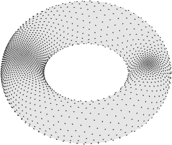
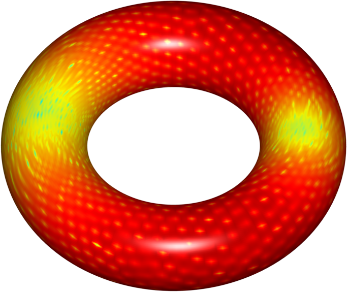
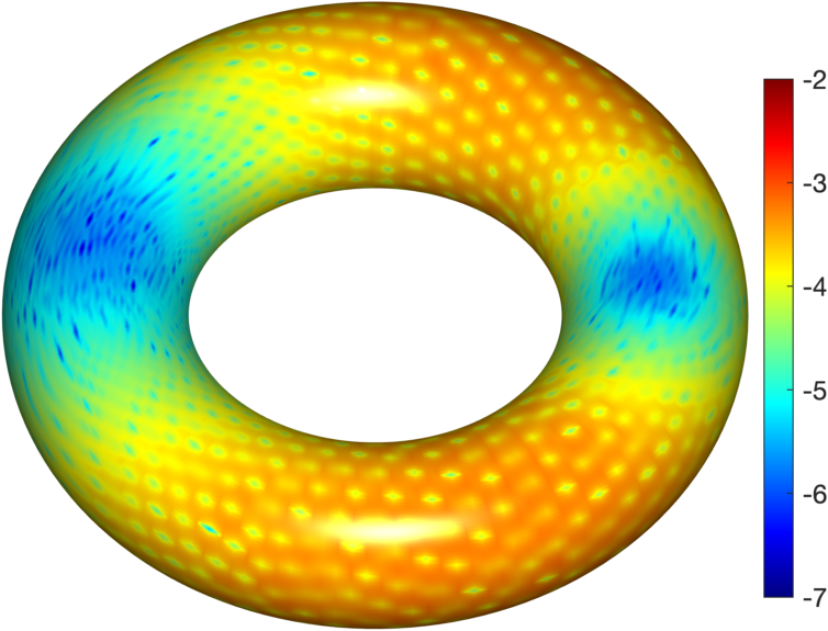
Figure 2. Left: Distribution of centers $\Xi$ on the torus. Middle and right: heat map of the power function $P_{\Xi}$ (displayed on a $\log_{10}$ scale) using the Matérn kernel with $s=4$ and $s=5$, respectively.

Proof.

For the local polynomial reproduction $a$ from Proposition 6.1 with $\epsilon=1/2$, we note that $a(\cdot,x)\in\mathbb{R}^{\Xi}$, so $P_{\Xi}(x)^{2}\leq\mathcal{Q}_{\Xi,x}(a(\cdot,x))$ follows by optimality. Since $\Phi$ is obtained as a restriction: $\Phi(x,y)=\phi(x-y)$, we have

$$\mathcal{Q}_{\Xi,x}(a(\cdot,x))=\phi(0)-2\sum_{\xi\in\Xi}a(\xi,x)\phi(x-\xi)+\sum_{\xi,\zeta\in\Xi}a(\xi,x)a(\zeta,x)\phi(\xi-\zeta).$$

Replacing every occurrence of $\phi$ with $p\in\mathcal{P}_{m}$ in this expression we have

$$\tilde{\mathcal{Q}}_{p}:=p(0)-2\sum_{\xi\in\Xi}a(\xi,x)p(x-\xi)+\sum_{\xi,\zeta\in\Xi}a(\xi,x)a(\zeta,x)p(\xi-\zeta)=0.$$

Thus $P_{\Xi}(x)^{2}\leq|\mathcal{Q}(a(\cdot,x))|=|\mathcal{Q}(a(\cdot,x))-\tilde{\mathcal{Q}_{p}}|$ holds, from which we obtain, by rearranging terms and applying the triangle inequality, the estimate

$$P_{\Xi}(x)^{2} \leq |\phi(0-p(0)|$$

$$+\,4\max_{\xi\in\Xi\cap B_{\mathbb{M}}(x,2\kappa h)}|\phi(x-\xi)-p(x-\xi)|$$

$$+\,4\max_{\xi,\zeta\in\Xi\cap B_{\mathbb{M}}(x,2\kappa h)}|\phi(\xi-\zeta)-p(\xi-\zeta)|.$$

The result now follows by noting that if $\operatorname{dist}_{\mathbb{M}}(\xi,\zeta)<4\kappa h$, then [14, Theorem 6] ensures $|\xi-\zeta|\leq Kh$ for some $K\propto\kappa$, and the fact that $\|\phi-p\|_{B(0,Kh)}\leq C(Kh)^{k}[\phi]_{k}$. ∎

From this, we have the pointwise bounds on the interpolation error for $f\in\mathcal{N}_{\Phi}$

(25) $$|f(x)-I_{\Xi}f(x)|\leq P_{\Xi}(x)\|f\|_{\mathcal{N}_{\Phi}}\leq C\Bigl{(}h(\Xi,\Omega)\Bigr{)}^{k/2}\|f\|_{\mathcal{N}_{\Phi}}.$$

Although there exist kernel interpolation results in more general settings (e.g., [14] treats compact, embedded Riemannian manifolds), such results generally employ a global fill distance $h_{\mathbb{M}}=\sup_{x\in\mathbb{M}}\operatorname{dist}_{\mathbb{M}}(x,\Xi)$, while the novelty of (25) is in its locality – the parameter $h(\Xi,\Omega)$ depends on the distribution of $\Xi\cap\Omega$ in a potentially small set $\Omega$.

This is illustrated by the numerical example displayed in Figure 2, where a finite point set $\Xi\subset\mathbb{M}$ is selected on the torus $\mathbb{M}$ (which is the zero set of a fourth degree polynomial in $\mathbb{R}^{3}$). Using the Matérn RBF of integer order $s$:

$$\phi(x)=|x|^{s-3/2}K_{s-3/2}(|x|)$$

we display the power function $P_{\Xi}$ for two different values $s$, noting it is significantly smaller in regions $\Omega$ where $h(\Xi;\Omega)$ shrinks. The Matérn RBF serves as a fundamental solution (up to a constant multiple) of $(1-\Delta)^{s}$ in $\mathbb{R}^{3}$, and thus its native space is $W_{2}^{s}(\mathbb{R}^{3})$. The restricted kernel $\Phi(x,y)=\phi(x-y)$ on the torus $\mathbb{M}$ has, by the trace theorem, native space $W_{2}^{s-1/2}(\mathbb{M})$.

We note that for the above choice of kernel $\phi\in C^{\infty}(\mathbb{R}^{3}\setminus\{0\})$, $\phi\in C^{2s-3-\epsilon}(\mathbb{R}^{3})$ for any $\epsilon>0$ but $\phi\notin C^{2s-3}(\mathbb{R}^{3})$. However, the asymptotic expansion [17, Example 4.2] shows that $\phi(x)=c|x|^{2s-3}+\psi(x)$, with $\psi\in C^{2s-3}(\mathbb{R}^{3})$, so $[\phi]_{2s-3}=1$. Thus in this case, Proposition 6.2 holds with $k=2s-3$.

6.2. MLS approximation

We consider (1), modified in the following way. For an algebraic manifold $\mathbb{M}$, with $\Omega\subset\mathbb{M}$, $\Xi\subset\Omega$ and $f\in C(\Omega)$, we define the MLS approximant

(26) $$\mathcal{M}_{\Xi}f(z)=p_{z}^{*}(z),\text{ where }p_{z}^{*}:=\arg\min_{p\in\mathcal{P}_{m}}\sum_{\xi\in\Xi}\left(p(\xi)-f(\xi)\right)^{2}\mathcal{W}(\xi,z)$$

by taking weight function $\mathcal{W}(\xi,z)=\Phi(\frac{|z-\xi|}{\delta})$. Note that this is simply (13) with $\varPi=\mathcal{P}_{m}$.

Remark 4.

We note that this weight function satisfies Assumption 4. In particular, using the Euclidean norm on $\mathbb{R}^{N}$, we have $F_{\xi}(z):=|z-\xi|$, and can estimate $\nabla^{k}F_{\xi}$ by the metric equivalence (4). Indeed, we have,

$$F_{\xi}(\mathrm{Exp}_{\xi}(x))=|\mathrm{Exp}_{\xi}(x)-\xi|=\left|\psi(x)\right|$$

where $\psi(x):=\mathrm{Exp}_{\xi}(x)-\xi$ is smooth (in fact, analytic since $\mathbb{M}$ is an algebraic manifold). By the chain rule and product rule, $D^{\alpha}F_{\xi}(\mathrm{Exp}_{\xi}(x))$ is a linear combination of functions of the form $h_{\beta}(\psi(x))\prod_{j=1}^{|\beta|}D^{\gamma_{j}}\psi(x)$ where $0<\beta\leq\alpha$, $\sum_{j=1}^{|\beta|}\gamma_{j}=\alpha$, and $h_{\beta}$ is the partial derivative of the Euclidean norm, $D^{\beta}(|y|)=h_{\beta}(y)$. Because each $h_{\beta}$ is homogeneous of order $1-|\beta|$ and $\psi$ is smooth, it follows that

$$\left|h_{\beta}(\psi(x))\prod_{j=1}^{|\beta|}D^{\gamma_{j}}\psi(x)\right|\leq C|\psi(x)|,$$

and, hence, $|D^{\alpha}F_{\xi}(\mathrm{Exp}_{\xi}(x))|\leq C|\psi(x)|^{1-|\alpha|}=C|\mathrm{Exp}_{\xi}(x)-\xi|^{1-|\alpha|}$. Finally, the metric equivalence (22) guarantees that (20) is satisfied.

From this, we have the following results, which match well-known results from the Euclidean setting, but are novel in the context of MLS approximation on manifolds. In the statement of the result, as well as its proof, we use the notation $D_{v}F(z)$ to denote the directional derivative of $F$ in the direction $v$ at $z$ ; for functions defined on a $\mathbb{R}^{N}$ neighborhood of $z$, this is the customary $\lim_{t\to 0}\frac{1}{t}(F(z+tv)-F(z))$, while for functions defined on $\mathbb{M}$ and $v\in T_{0}^{1}\mathbb{M}_{z}$, this is $\nabla F(z)v$.

Proposition 6.3.

For a compact subset $\Omega\subset\mathbb{M}$ with Lipschitz boundary and any $\rho_{0}>1$, there is a constant $C$ so that, for any sufficiently dense $\Xi\subset\Omega$ which satisfies $\rho:=\frac{h}{q}\leq\rho_{0}$, we have for any $k\leq m+1$ and $f\in C^{k}(\Omega)$, that

$$\left|f(z)-\mathcal{M}_{\Xi}f(z)\right|\leq C\delta^{k}\|f\|_{C^{k}(\Omega)}$$

and for any unit tangent vector $v\in T_{0}^{1}\mathbb{M}_{z}$ at $z$, we have

$$\left|D_{v}f(z)-D_{v}\mathcal{M}_{\Xi}f(z)\right|\leq C\delta^{k-1}\|f\|_{C^{k}(\Omega)}$$

Proof.

We have the standard estimate

$$\left|f(z)-\mathcal{M}_{\Xi}f(z)\right| \leq\left|f(z)-p(z)\right|+\left|\mathcal{M}_{\Xi}p(z)-\mathcal{M}_{\Xi}f(z)\right|$$

$$\leq\left(1+\sum_{\xi\in\Xi}|b^{\star}(\xi,z)|\right)\inf_{p\in\mathcal{P}_{m}}\|f-p\|_{L_{\infty}(\Omega\cap B(z,\delta))}.$$

Note that $\sum_{\xi\in\Xi}|b^{\star}(\xi,z)|$ is bounded by Lemma 5.1. If $f\in C^{k}(\Omega)$, then we can take an extension $\mathcal{E}f\in C^{k}(W)$ defined on a neighborhood $W$ of $\Omega$ in $\mathbb{R}^{N}$ with $\|\mathcal{E}f\|_{C^{k}(W)}\leq C\|f\|_{C^{k}(\Omega)}$. Thus,

$$\|f-p\|_{L_{\infty}(\Omega\cap B(z,\delta))}\leq\|\mathcal{E}f-p\|_{L_{\infty}(W\cap B_{\mathfrak{E}}(z,\delta))}\leq\delta^{k}\|\mathcal{E}f\|_{C^{k}(W)}\leq\delta^{k}\|f\|_{C^{k}(\Omega)}.$$

In a similar way, we may write

$$|\nabla f(z)v-\nabla\mathcal{M}f(z)v|=|\nabla f(z)v-\nabla p(z)v|+\|\nabla\mathcal{M}(f-p)(z)\|_{T_{1}^{0}\mathbb{M}_{z}}.$$

The second expression is bounded by $\sum_{\xi\in\Xi}\|\nabla b^{\star}(\xi,z)\|\|f-p\|_{L_{\infty}(\Omega\cap B(z,\delta))}$, while the first can be controlled by directional derivative $|D_{v}\mathcal{E}f(z)-D_{v}p(z)|$ since both functions $\mathcal{E}f$ and $p$ are defined on $W$. Thus,

$$|\nabla f(z)v-\nabla\mathcal{M}f(z)v| \leq \inf_{p\in\mathcal{P}_{m}}|D_{v}\mathcal{E}f(z)-D_{v}p(z)|+\frac{C}{h}\|\mathcal{E}f-p\|_{L_{\infty}(W\cap B_{\mathfrak{E}}(z,\delta))}$$

$$\leq C\delta^{k-1}\|f\|_{C^{k}(\Omega)}$$

and the result follows. ∎

6.2.1. Treating noisy data

We note that (26) can treat data $Y=(\xi,y_{\xi})_{\xi\in\Xi}$ directly. If $y_{\xi}=f(\xi)+\epsilon_{\xi}$ is perturbed by noise, say by independent, identically distributed $\epsilon_{\xi}\sim\mathcal{N}(0,\sigma^{2})$, then we may write

$$\mathcal{M}_{\Xi}(Y)(z) :=\sum_{\genfrac{}{}{0.0pt}{}{\xi\in\Xi}{\mathcal{W}(\xi,z)>0}}b^{\star}(\xi,z)y_{\xi}=\sum_{\genfrac{}{}{0.0pt}{}{\xi\in\Xi}{\mathcal{W}(\xi,z)>0}}b^{\star}(\xi,z)f(\xi)+\sum_{\genfrac{}{}{0.0pt}{}{\xi\in\Xi}{\mathcal{W}(\xi,z)>0}}b^{\star}(\xi,z)\epsilon_{\xi}$$

$$=\mathcal{M}_{\Xi}(f)(z)+\sum_{\genfrac{}{}{0.0pt}{}{\xi\in\Xi}{\mathcal{W}(\xi,z)>0}}b^{\star}(\xi,z)\epsilon_{\xi}$$

Now using linearity of expectation, and the fact that $\mathbb{E}\left[\epsilon_{\xi}\right]=0$, we get

$$\mathbb{E}\left[\left(f(z)-\mathcal{M}_{\Xi}(Y)(z)\right)^{2}\right] =\left(f(z)-\mathcal{M}_{\Xi}(f)(z)\right)^{2}+\mathbb{E}\left[\left(\sum_{\genfrac{}{}{0.0pt}{}{\xi\in\Xi}{\mathcal{W}(\xi,z)>0}}b^{\star}(\xi,z)\epsilon_{\xi}\right)^{2}\right].$$

Expressing $\bigl{(}\sum_{\genfrac{}{}{0.0pt}{}{\xi\in\Xi}{\mathcal{W}(\xi,z)>0}}b^{\star}(\xi,z)\epsilon_{\xi}\bigr{)}^{2}$ as $\sum_{\genfrac{}{}{0.0pt}{}{\xi,\xi^{\prime}\in\Xi}{\mathcal{W}(\xi,z)\mathcal{W}(\xi^{\prime},z)>0}}b^{\star}(\xi,z)b^{\star}(\xi^{\prime},z)\epsilon_{\xi}\epsilon_{\xi^{\prime}}$, we treat the second term as

$$\mathbb{E}\left[\left(\sum_{\genfrac{}{}{0.0pt}{}{\xi\in\Xi}{\mathcal{W}(\xi,z)>0}}b^{\star}(\xi,z)\epsilon_{\xi}\right)^{2}\right] =\sigma^{2}\sum_{\genfrac{}{}{0.0pt}{}{\xi\in\Xi}{\mathcal{W}(\xi,z)>0}}|b^{\star}(\xi,z)|^{2}\leq\sigma^{2}\left(\sum_{\xi\in\Xi}|b^{\star}(\xi,z)|\right)^{2}\leq 16C^{2}\rho^{2d}\sigma^{2}.$$

This shows for the mean squared error (MSE) the bound

$$\mathbb{E}\left[\left(f(z)-\mathcal{M}_{\Xi}(Y)(z)\right)^{2}\right]\leq\left(f(z)-\mathcal{M}_{\Xi}(f)(z)\right)^{2}+16C^{2}\rho^{2d}\sigma^{2}.$$

7. Numerical experiments for MLS

In this section, we numerically demonstrate the MLS approximation stability and error estimates from the previous section. Before presenting these results, we discuss the algorithm used to produce the MLS approximants.

7.1. MLS method for approximation on manifolds

We describe our method for constructing MLS approximants for two dimensional algebraic manifolds $\mathbb{M}\subset\mathbb{R}^{3}$, the generalization to higher dimensional manifolds should be straightforward. To make the method general and easy to implement, we want to work with the ambient polynomial space $\mathcal{P}_{m}(\mathbb{R}^{3})$ of total degree $m$. The issue with this is that depending on $m$ and the degree of the algebraic manifold, this can lead to rank deficiency in the local least squares problems inherent to (26) since the dimension of $\mathcal{P}_{m}(\mathbb{R}^{3})$ may be larger than the dimension of $\mathcal{P}_{m}(\mathbb{M})$. To further elucidate the issue we first work out the the exact dimension $\mathcal{P}_{m}(\mathbb{M})$ using some results from algebraic geometry.

The dimension of $\mathcal{P}_{m}(\mathbb{M})$

The algebra of polynomials on $\mathbb{M}\subset\mathbb{R}^{N}$ can be expressed as a quotient $\mathcal{P}(\mathbb{M})=\mathcal{P}(\mathbb{R}^{N})/I(\mathbb{M})$, with the help of the ideal

$$I(\mathbb{M}):=\{p\in\mathcal{P}(\mathbb{R}^{N})\mid p|_{\mathbb{M}}=0\}.$$

The map $m\mapsto\dim\bigl{(}\mathcal{P}_{m}(\mathbb{M})\bigr{)}$ is called the Hilbert function of $I(\mathbb{M})$. In this case, $\mathcal{P}_{m}(\mathbb{M})=\mathcal{P}_{m}(\mathbb{R}^{N})/I_{m}(\mathbb{M})$, where $I_{m}(\mathbb{M}):=I(\mathbb{M})\cap\mathcal{P}_{m}(\mathbb{R}^{N})$. Thus

$$\dim(\mathcal{P}_{m}(\mathbb{M}))=\dim\bigl{(}\mathcal{P}_{m}(\mathbb{R}^{N})/I_{m}(\mathbb{M})\bigr{)}=\dim(\mathcal{P}_{m}(\mathbb{R}^{N}))-\dim(I_{m}(\mathbb{M})).$$

This observation is enough to cleanly handle the case of algebraic hypersurfaces in $\mathbb{R}^{N}$ if $\mathbb{M}=\{x\in\mathbb{R}^{N}\mid P(x)=0\}$ and $P$ is irreducible. In that case,

$$I(\mathbb{M})=\{qP\mid q\in\mathcal{P}(\mathbb{R}^{N})\}.$$

In other words, $I(\mathbb{M})$ can be expressed as the ideal generated by $P$. Consequently, $I_{m}(\mathbb{M})=\{qP\mid\deg(qP)\leq m\}$. Writing $k:=\deg(P)$, we then have, for $m\geq k$, that $\dim(I_{m}(\mathbb{M}))=\dim(\mathcal{P}_{m-k})(\mathbb{R}^{N})$, while for $m<k$, t $\dim(I_{m}(\mathbb{M}))=0$. Thus,

(27) $$\dim(\mathcal{P}_{m}(\mathbb{M}))=\begin{cases}\begin{pmatrix}N+m\\ N\end{pmatrix}-\begin{pmatrix}N+m-k\\ N\end{pmatrix}&\text{for $m\geq k$}\\ \qquad\begin{pmatrix}N+m\\ N\end{pmatrix}&\text{for $m<k$.}\end{cases}$$

The situation for $N-d\geq 2$ (varieties of codimension greater than one) is more complicated, but no less well understood. We refer the reader to [9] for precise details.

Selecting the parameter $\delta$

The support parameter defines the local subsets of points of $\Xi\subset\Omega$ for the weighted least squares problem for each evaluation point $x\in X\subset\Omega$; we denote these subsets as $\Xi_{x}(\delta)$. Given $m$ and the set of evaluation points $X$ to compute the approximant, $\delta$ should be chosen so that $N_{\Xi_{x}}=\#\Xi_{x}(\delta)$ is larger than the dimension of the polynomial space being used in the approximation.

Since we use the ambient space $\mathcal{P}_{m}(\mathbb{R}^{3})$ to construct the MLS approximants, we require that $N_{\Xi_{x}}>\dim(\mathcal{P}_{m}(\mathbb{R}^{3}))=M$. To ensure that this holds, we use the following procedure. For each $x$ we determine the $2M$ nearest neighbors from $\Xi$ to $x$ and follow this by computing the minimum radius of the ball in $\mathbb{R}^{3}$ centered at $x$ that contains all these nearest neighbors. We then choose $\delta$ as the maximum of these minimum radii for all $x\in X$. In our experiments this guaranteed that $N_{\Xi_{x}}\geq 2M$, for all $x$. Note that determining $\delta$ with this procedure can be done efficiently using $k$-d tree.

Singular value decomposition

To deal with the issue of rank deficiency of MLS problem (26) that can arise from a dimension mismatch between $\mathcal{P}_{m}(\mathbb{R}^{3})$ and $\mathcal{P}_{m}(\mathbb{M})$, we use the singular value decomposition (SVD) of the Vandermonde matrix formed from evaluating a basis for $\mathcal{P}_{m}(\mathbb{R}^{3})$ at $\Xi_{x}(\delta)$. An important step in this process is choosing the basis for $\mathcal{P}_{m}(\mathbb{R}^{3})$, for which we propose using one that depends on $\Xi_{x}(\delta)$ as follows. Let $\{p_{j}\}_{j=1}^{M}$ denote the standard monomial basis for $\mathcal{P}_{m}(\mathbb{R}^{3})$ and select the basis for the MLS approximant on $\Xi_{x}(\delta)$ as $\{p_{j}((\cdot-x)/\delta)\}_{j=1}^{M}$. We denote the Vandermonde matrix formed by evaluating this basis at $\Xi_{x}$ as $\mathbf{P}_{\Xi_{x}}$.

Using the the procedure for choosing $\delta$ described above, this Vandermonde matrix is overdetermined, with $M$ columns and $N_{\Xi_{x}}\geq 2M$ rows. We denote the (reduced) SVD of $\mathbf{P}_{\Xi_{x}}$ as

$$\mathbf{P}_{\Xi_{x}}=\mathbf{U}_{\Xi_{x}}\boldsymbol{\Sigma}_{\Xi_{x}}\mathbf{V}_{\Xi_{x}}^{T},$$

where the $M$ columns of $\mathbf{U}_{\Xi_{x}}$ are orthonormal, $\mathbf{V}_{\Xi_{x}}$ is an $M$-by-$M$ orthogonal matrix, and $\boldsymbol{\Sigma}_{\Xi_{x}}=\text{diag}(\sigma_{1},\ldots,\sigma_{M})$. To determine a discretely orthonormal basis for $\mathcal{P}_{m}(\Xi_{x}(\delta))$, we use the first $K$ columns of $\mathbf{U}_{\Xi_{x}}$ corresponding to the numerical rank of $\mathbf{P}_{\Xi_{x}}$. This discrete orthonormal basis, together with the similarly reduced $\mathbf{V}_{\Xi_{x}}$ and $\boldsymbol{\Sigma}_{\Xi_{x}}$ can then be used directly to solve the optimization problem (26).

Since $N_{\Xi_{x}}$ is much less that $N_{\Xi}$ and does not grow as $\Xi$ increases, the procedure is efficient (and is pleasingly parallel). It also allows one to work entirely with ambient polynomial space and the algorithm finds out both the (numerical) dimension of the space of restricted polynomials and a basis for this space automatically.

Weight function

The final piece for the MLS problem is the weight function, for which we use the $C^{4}(\mathbb{R}^{3})$ Wendland kernel

$$w(\xi,\zeta)=\left(1-\dfrac{|\xi-\zeta|}{\delta}\right)_{+}^{6}\left(1+6\left(\dfrac{|\xi-\zeta|}{\delta}\right)+\frac{35}{3}\left(\dfrac{|\xi-\zeta|}{\delta}\right)^{2}\right).$$

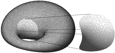
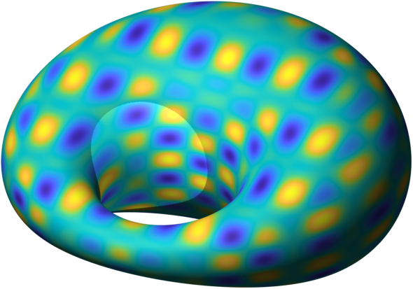
Figure 3. Left panel: visualization of the manifold $\mathbb{M}$ and the compact subset $\widehat{\Omega}\subset\mathbb{M}$ (inset) used in the MLS numerical experiments; see (28) and (29) for exact definitions. Black solid spheres mark the node sets $\Xi$ on $\mathbb{M}$ and $\widehat{\Xi}$ on $\widehat{\Omega}$. Right panel: heat map of the target function on $\mathbb{M}$ considered in the numerical experiments; the brighter region highlights the target function on $\widehat{\Omega}$.

7.2. Verification of error and stability estimates

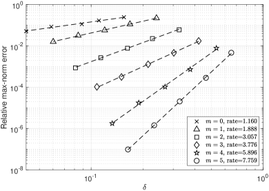
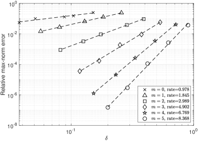
(a)	(b)

Figure 4. Convergence results where the approximation problem is done over (a) all of $\mathbb{M}$ and (b) only the compact subset $\widehat{\Omega}$. The estimated rates of convergence for each $m$ are included in legend labels.

Consider the following two-dimensional, degree four algebraic manifold:

(28) $$\mathbb{M}=\left\{x=(x_{1},x_{2},x_{3})\in\mathbb{R}^{3}\;\left|\left(x_{1}^{2}+x_{2}^{2}+x_{3}^{2}-d^{2}+b^{2}\right)^{2}-4\left(ax_{1}+cd\right)^{2}-4b^{2}x_{2}^{2}=0\right.\right\},$$

where $a=2$, $b=1.9$, $d=1$, and $c^{2}=a^{2}-b^{2}$; this manifold is an example of a cyclide of Dupin. We test the stability and error estimates of MLS approximations over the whole manifold, i.e., $\Omega=\mathbb{M}$, and over the compact subset of $\mathbb{M}$ defined as

(29) $$\widehat{\Omega}=\mathbb{M}\cap B_{1}(\xi_{\rm c}),$$

where $B_{1}(\xi_{\rm c})$ is the ball in $\mathbb{R}^{3}$ of radius 1 centered at the point $\xi_{\rm c}=(0,\sqrt{9-6a+b^{2}},0)$ on the cyclide; see the left panel of Figure 3 for an illustration of $\mathbb{M}$ and $\widehat{\Omega}$. For the target function, we use the following $C^{\infty}$ function defined in $\mathbb{R}^{3}$ and restricted $\mathbb{M}$

(30) $$f(x)=\cos(\pi(x_{1}-\frac{3}{10}))\sin(2\pi(x_{2}-\frac{1}{5}))\cos(3\pi(x_{3}-\frac{1}{10}));$$

see the right panel of Figure 3 for an illustration of $f$.

To test the error estimates from Proposition 6.3, we consider MLS approximants constructed from samples of (30) at unstructured, quasi-uniform point sets $\Xi\subset\mathbb{M}$ of cardinalities $N_{\Xi}=2^{i}$, $i=14,\ldots,18$. We also consider approximants of (30) from restrictions of these point sets to $\widehat{\Omega}$, i.e., $\widehat{\Xi}:=\Xi\cap\widehat{\Omega}$, which results in point sets of cardinalities $N_{\widehat{\Xi}}=706,\,1399,\,2838,\,5655,\,11308$. See the left panel of Figure 3 for an illustration of these points with $N_{\Xi}=2^{14}$ and $N_{\widehat{\Xi}}=706$ nodes. The error in MLS approximants for $\Omega$ are computed at a finer set of $N_{X}=2^{21}$ evaluation points $X\subset\mathbb{M}$, while approximants on $\widehat{\Omega}$ are computed at $N_{\widehat{X}}=86123$ evaluation points $\widehat{X}=X\cap\widehat{\Omega}$.

The convergence results using the set-up described above are given in Figure 4 for polynomial degrees $m=0,1,\ldots,5$. Included in these results are the estimated rates of convergence computed from a line of best fit of the (log) of the data. The convergence rates are estimated in terms of $\delta$, which should be proportional to the mesh-norm of $\Xi$ since these point sets are quasi-uniform. We see for the MLS approximants over all of $\mathbb{M}$ that the estimated convergence rates are close to the optimal rates of $m+1$ expected from Proposition 6.3 in the case of $m=0,1,2,3$, but that for $m=4$ and $5$ the rates are higher by about 1. Similar results hold for MLS approximants over $\widehat{\Omega}$, but in this case we observe higher rates also for $m=3$. These numerical results back up the new theoretical results that one can use MLS entirely locally and still obtain similar convergence rates to working globally on a manifold.

We note that the cyclide surface is defined by the level surface of an irreducible polynomial of degree $k=4$. Thus, by (27) above, the dimension of $\mathcal{P}_{m}(\mathbb{M})$ is given by:

$$\dim(\mathcal{P}_{m}(\mathbb{M}))=\begin{cases}2m^{2}+2&m\geq 4\\ \frac{1}{6}(m+3)(m+2)(m+1)&m<4.\end{cases}.$$

In the numerical experiments from Figure 4 (as well as many others not presented here), we observed that the SVD procedure described in Section 7.1 consistently produced a discrete orthogonal basis for each $\mathcal{P}_{m}(\Xi_{x}(\delta)))$ that matched the expected dimension from the formula above. This numerical evidence supports the robustness and generality of this relatively simple and straightforward method of working with polynomials in the ambient space.

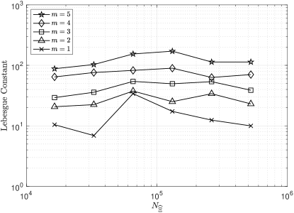
Figure 5. Numerically computed Lebesgue constants for the MLS approximation problem for the compact subset $\widehat{\Omega}$ of cyclide using quasi-uniform points of increasing cardinality $N_{\widehat{\Xi}}$.

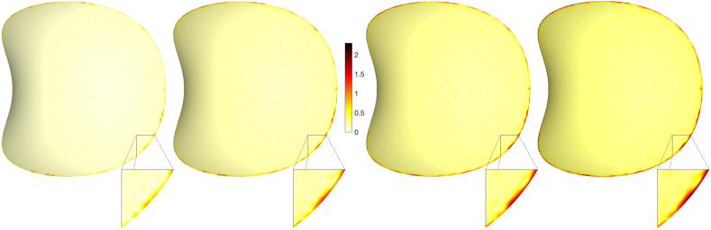
Figure 6. Lebesgue functions of the MLS approximants on $\widehat{\Omega}$ using a point set with $N_{\widehat{\Xi}}=5655$ and (from left to right) polynomial degrees $m=2,3,4,5$. Note that the color scheme is same for each plot according to the given colorbar and is based on the $\log_{10}$ of the values of the Lebesgue functions.

	Perturbation $\sigma=10^{-2}$		Perturbation $\sigma=10^{-1}$
Deg.	Mean diff.	Std Dev	Mean diff.	Std Dev
Approximation on $\Omega$
$0$	$4.49\times 10^{-2}$	$2.94\times 10^{-3}$	$4.53\times 10^{-1}$	$2.85\times 10^{-2}$
$1$	$8.59\times 10^{-2}$	$2.68\times 10^{-2}$	$8.77\times 10^{-1}$	$2.70\times 10^{-1}$
$2$	$5.05\times 10^{-2}$	$4.25\times 10^{-3}$	$5.07\times 10^{-1}$	$5.84\times 10^{-2}$
$3$	$4.50\times 10^{-2}$	$3.26\times 10^{-3}$	$4.46\times 10^{-1}$	$3.86\times 10^{-2}$
$4$	$4.04\times 10^{-2}$	$2.91\times 10^{-3}$	$4.04\times 10^{-1}$	$2.78\times 10^{-2}$
$5$	$3.67\times 10^{-2}$	$2.36\times 10^{-3}$	$3.61\times 10^{-1}$	$2.16\times 10^{-2}$
Approximation on $\widehat{\Omega}$
$0$	$3.89\times 10^{-2}$	$2.78\times 10^{-3}$	$3.88\times 10^{-1}$	$3.23\times 10^{-2}$
$1$	$3.14\times 10^{-2}$	$3.18\times 10^{-3}$	$3.07\times 10^{-1}$	$3.11\times 10^{-2}$
$2$	$3.01\times 10^{-2}$	$2.21\times 10^{-3}$	$2.95\times 10^{-1}$	$2.56\times 10^{-2}$
$3$	$2.69\times 10^{-2}$	$2.31\times 10^{-3}$	$2.67\times 10^{-1}$	$2.12\times 10^{-2}$
$4$	$2.60\times 10^{-2}$	$2.57\times 10^{-3}$	$2.61\times 10^{-1}$	$2.72\times 10^{-2}$
$5$	$2.53\times 10^{-2}$	$2.58\times 10^{-3}$	$2.59\times 10^{-1}$	$3.13\times 10^{-2}$

Table 1. Stability of the MLS approximation under noise introduced to the target function (30). Noise was added to the samples of the target function as $\tilde{f}_{j}=f_{j}+\epsilon_{j}$, where $\epsilon_{j}\sim\mathcal{N}(0,\sigma)$. MLS approximants of $\tilde{f}_{j}$ were computed using 100 different trials and results show the mean and standard deviation of max-norm differences between the MLS approximants and the exact function. Computations for $\Omega$ were done using $\widehat{\Xi}$ with $N_{\Xi}=262144$ and the errors were measured at $2097152$ points over $\Omega$, while computations for $\widehat{\Omega}$ were done using $\widehat{\Xi}\subset\widehat{\Omega}$ with $N_{\widehat{\Xi}}=11308$ and the errors were measured at $86123$ points over $\widehat{\Omega}$

We conclude with some experiments on the stability of the MLS approximants. These are illustrated as follows:

1. Table 1 displays results of experiments where the data is perturbed by different levels of noise. As expected from the discussion in Section 6.2.1, we see that the errors in the MLS approximants are closely controlled by the noise level.

2. Figure 5 displays the numerically computed Lebesgue constants for the MLS approximants on $\widehat{\Omega}$. We see that the Lebesgue constants appear to remain bounded as expected from the results given in Section 5.1.

3. Figure 6 gives visualizations of the the Lebesgue functions on $\widehat{\Omega}$ for different polynomial degrees. These images show that the Lebesgue functions are largest along the boundary of the domain and increase with increasing $m$, which is also the typical behavior in planar domains.

7.3. Meshed surface

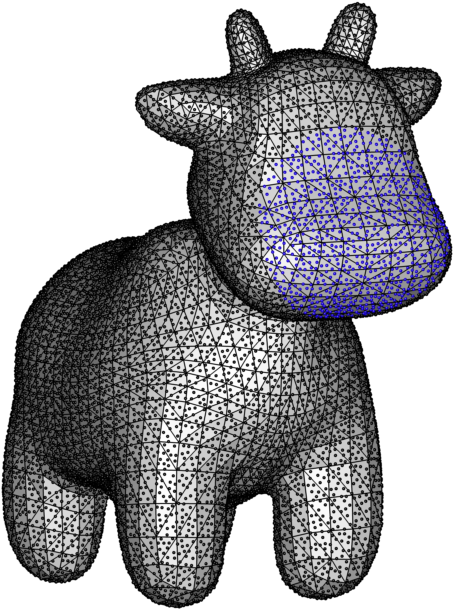
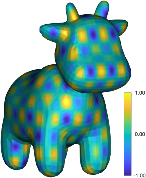
(a)	(b)
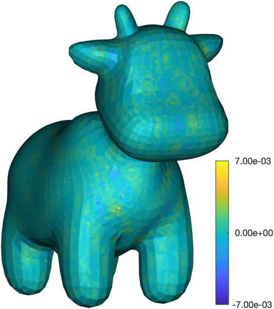
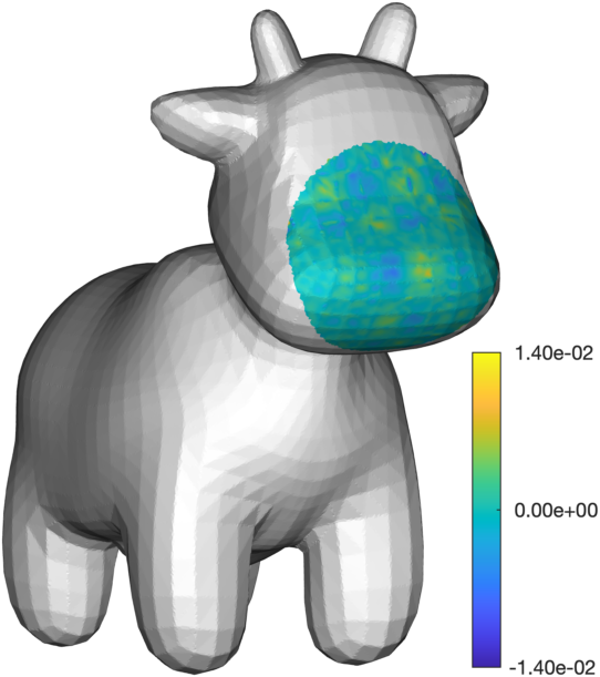
(c)	(d)

Figure 7. (a) Visualization of the piecewise algebraic Spot manifold $\mathbb{M}$ and the compact subset $\widehat{\Omega}\subset\mathbb{M}$ (highlighted by the blue points) in the MLS numerical experiments. (b) Heat map of the target function on $\mathbb{M}$ considered in the numerical experiments. (c) & (d) Heat map of the errors in the $m=3$ MLS approximants of the target function when using all points on $\mathbb{M}$ a restrictions of the points to $\widehat{\Omega}$.

We lastly explore the behavior of the MLS method on a manifold that is not covered by our theory. For this we use the piecewise algebraic “Spot” manifold $\mathbb{M}$ from [7], which is defined by a triangulated mesh consisting of 2930 vertices. We employ the same algorithmic approach as the previous section. That is, we use global polynomials restricted to the surface, and again consider both the whole manifold, i.e., $\Omega=\mathbb{M}$ and a compact subset of $\mathbb{M}$ defined as

(31) $$\widehat{\Omega}=\mathbb{M}\cap B_{\frac{3}{10}}(\xi_{\rm c}),$$

where $B_{\frac{3}{10}}(\xi_{\rm c})$ is the ball in $\mathbb{R}^{3}$ of radius $\frac{3}{10}$ centered on the nose of Spot. See Figure 7 (a) for a visualization of Spot and the subdomain $\widehat{\Omega}$.

We consider MLS approximations of the target function

(32) $$f(x)=\cos(6\pi x_{1})\sin(9\pi(x_{2}-\frac{1}{10}))\cos(7\pi x_{3})$$

on $\mathbb{M}$ and $\widehat{\Omega}$, which is displayed in Figure 7 (b). We use samples of $f$ on a quasi-uniform node set $\Xi\subset\mathbb{M}$ with $N_{\Xi}=32768$ and the restriction of this set $\widehat{\Xi}\subset\widehat{\Omega}$ with $N_{\widehat{\Xi}}=1671$. The evaluation points $X$ and $\widehat{X}$ are chosen to densely sample the approximants on the respective domains.

Figure (c) & (d) show the errors in the MLS approximation using $m=3$ degree polynomials for $\mathbb{M}$ and $\widehat{\Omega}$, respectively. We see that the approximations in both settings provide good reconstructions of the target. The dimension of the polynomials restricted to the surface were similarly determined by an SVD. However, we found that the point sets were too coarse compared to the resolution of the Spot mesh to reveal the 2-dimensional surface structure and that the dimension of the polynomial space matched the ambient 3-dimensional space in all cases. This suggests an immense flexibility of the proposed MLS method even for non-algebraic surfaces. Instead of breaking down, it essentially works as a standard 3-dimensional MLS approximation based on a point cloud.

While not presented here, we also observed convergence similar to the previous section for the MLS approximants as the density of the node sets $\Xi$ and $\widehat{\Xi}$ was increased. While we do not yet have theoretical guarantees concerning the accuracy and stability of the method in the ambient space, these numerical results are nevertheless promising. They suggest that the proposed method is robust even in a pre-asymptotic regime and can be employed in a variety of applications.

A contribution of this paper is to show both theoretically and practically convergence of the MLS in the asymptotic limit of many centers. In this limit, the structure of the manifold will be captured also by the restriction of ambient space polynomials.

Acknowledgements

The authors wish to thank Daniel Erman for helpful comments regarding the Hilbert function. Grady Wright was supported by grant DMS-2309712 from the US National Science Foundation. Thomas Hangelbroek was supported by by grant DMS-2010051 from the US National Science Foundation.

References

- [1] George Backus and Freeman Gilbert. The resolving power of gross earth data. Geophysical Journal International, 16(2):169–205, 1968.
- [2] Víctor Bayona. Comparison of moving least squares and rbf+ poly for interpolation and derivative approximation. Journal of Scientific Computing, 81:486–512, 2019.
- [3] Ted Belytschko, Y. Y. Lu, and Lei Gu. Element‐free galerkin methods. International Journal for Numerical Methods in Engineering, 37:229–256, 1994.
- [4] L. Bos, N. Levenberg, P. Milman, and B. A. Taylor. Tangential Markov inequalities characterize algebraic submanifolds of . Indiana University Mathematics Journal, 44(1):115–138, 1995.
- [5] L. Bos and P. Milman. Tangential Markov inequalities on singular varieties. Indiana University Mathematics Journal, 55(1):65–73, 2006.
- [6] L. P. Bos, N. Levenberg, P. D. Milman, and B. A. Taylor. Tangential Markov inequalities on real algebraic varieties. Indiana University Mathematics Journal, 47(4):1257–1272, 1998.
- [7] Keenan Crane, Ulrich Pinkall, and Peter Schröder. Robust fairing via conformal curvature flow. ACM Transactions on Graphics (TOG), 32(4):1–10, 2013.
- [8] Feng Dai, Andriy Prymak, Alexei Shadrin, Vladimir Temlyakov, and Serguey Tikhonov. Entropy numbers and marcinkiewicz-type discretization. Journal of Functional Analysis, 281(6):109090, 2021.
- [9] Donal O’Shea David A. Cox, John Little. Ideals, Varieties, and Algorithms. Undergraduate Texts in Mathematics. Springer Cham, 2015.
- [10] Ronald DeVore and Amos Ron. Approximation using scattered shifts of a multivariate function. Transactions of the American Mathematical Society, 362(12):6205–6229, 2010.
- [11] Harold Donnelly and Charles Fefferman. Nodal sets of eigenfunctions on Riemannian manifolds. Invent. Math., 93(1):161–183, 1988.
- [12] Reinhard Farwig. Multivariate interpolation of arbitrarily spaced data by moving least squares methods. J. Comput. Appl. Math., 16(1):79–93, 1986.
- [13] Charles Fefferman and Raghavan Narasimhan. A local Bernstein inequality on real algebraic varieties. Mathematische Zeitschrift, 223:673–692, 1996.
- [14] Edward Fuselier and Grady B Wright. Scattered data interpolation on embedded submanifolds with restricted positive definite kernels: Sobolev error estimates. SIAM Journal on Numerical Analysis, 50(3):1753–1776, 2012.
- [15] Thomas Hangelbroek, Francis J Narcowich, and Joseph D Ward. Kernel approximation on manifolds I: bounding the Lebesgue constant. SIAM Journal on Mathematical Analysis, 42(4):1732–1760, 2010.
- [16] Thomas Hangelbroek, Francis J Narcowich, and Joseph D Ward. Polyharmonic and related kernels on manifolds: interpolation and approximation. Foundations of Computational Mathematics, 12:625–670, 2012.
- [17] Thomas Hangelbroek and Christian Rieger. Extending error bounds for radial basis function interpolation to measuring the error in higher order Sobolev norms. Mathematics of Computation, 94(351):381–407, 2025.
- [18] Thomas Hangelbroek and Dominik Schmid. Surface spline approximation on so (3). Applied and Computational Harmonic Analysis, 31(2):169–184, 2011.
- [19] Sigurdur Helgason. Differential geometry, Lie groups, and symmetric spaces. Academic press, 1979.
- [20] Kerstin Hesse and QT Le Gia. Local radial basis function approximation on the sphere. Bulletin of the Australian Mathematical Society, 77(2):197–224, 2008.
- [21] Ralf Hielscher and Tim Pöschl. An optimal ansatz space for moving least squares approximation on spheres. arXiv preprint arXiv:2310.15570, 2023.
- [22] Kurt Jetter, Joachim Stöckler, and Joseph Ward. Error estimates for scattered data interpolation on spheres. Mathematics of Computation, 68(226):733–747, 1999.
- [23] Andrew M Jones, Peter A Bosler, Paul A Kuberry, and Grady B Wright. Generalized moving least squares vs. radial basis function finite difference methods for approximating surface derivatives. Computers & Mathematics with Applications, 147:1–13, 2023.
- [24] András Kroó. Markov-type inequalities for surface gradients of multivariate polynomials. Journal of Approximation Theory, 118(2):235–245, 2002.
- [25] Peter Lancaster and Kestutis Salkauskas. Surfaces generated by moving least squares methods. Mathematics of Computation, 37:141–158, 1981.
- [26] David Levin. The approximation power of moving least-squares. Mathematics of computation, 67(224):1517–1531, 1998.
- [27] Wing-Kam Liu, Shaofan Li, and Ted Belytschko. Moving least-square reproducing kernel methods. I. Methodology and convergence. Comput. Methods Appl. Mech. Engrg., 143(1-2):113–154, 1997.
- [28] WR Madych and EH Potter. An estimate for multivariate interpolation. Journal of approximation theory, 43(2):132–139, 1985.
- [29] Davoud Mirzaei, Robert Schaback, and Mehdi Dehghan. On generalized moving least squares and diffuse derivatives. IMA Journal of Numerical Analysis, 32(3):983–1000, 2012.
- [30] Christian Rieger and Holger Wendland. Sampling inequalities for sparse grids. Numerische Mathematik, 136:439–466, 2017.
- [31] Christian Rieger and Barbara Zwicknagl. Sampling inequalities for infinitely smooth functions, with applications to interpolation and machine learning. Advances in Computational Mathematics, 32:103–129, 2010.
- [32] Donald Shepard. A two-dimensional interpolation function for irregularly-spaced data. In Proceedings of the 1968 23rd ACM National Conference, ACM ’68, page 517–524, New York, NY, USA, 1968. Association for Computing Machinery.
- [33] Barak Sober, Yariv Aizenbud, and David Levin. Approximation of functions over manifolds: a moving least-squares approach. J. Comput. Appl. Math., 383:Paper No. 113140, 20, 2021.
- [34] Nathaniel Trask, Martin Maxey, and Xiaozhe Hu. Compact moving least squares: an optimization framework for generating high-order compact meshless discretizations. Journal of Computational Physics, 326:596–611, 2016.
- [35] VS Videnskii. Extremal estimate for the derivative of a trigonometric polynomial on an interval shorter than its period. In Doklady Akademii Nauk, volume 130, pages 13–16, 1960.
- [36] Holger Wendland. Local polynomial reproduction and moving least squares approximation. IMA Journal of Numerical Analysis, 21(1):285–300, 2001.
- [37] Holger Wendland. Moving least squares approximation on the sphere. Mathematical Methods for Curves and Surfaces, Vanderbilt Univ. Press, Nashville, TN, pages 517–526, 2001.
- [38] Zong-min Wu and Robert Schaback. Local error estimates for radial basis function interpolation of scattered data. IMA journal of Numerical Analysis, 13(1):13–27, 1993.